Embed Size (px)
Citation preview
Fast Spectral Transforms and Logic Synthesis
DoRon Motter
August 2, 2001
Introduction
• Truth Table Representation– Value provides complete information for one
combination of input variables
– Provides no information about other combinations
• Spectral Representation– Value provides some information about the behavior of
the function at multiple points
– Does not contain complete information about any single point

Spectral Transformation
• Synthesis– Many algorithms proposed leveraging fast
transformation
• Verification– Correctness may be checked more efficiently
using a spectral representation.
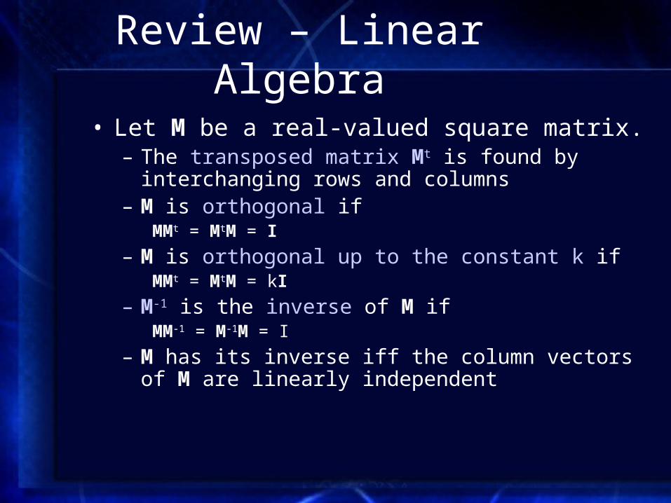
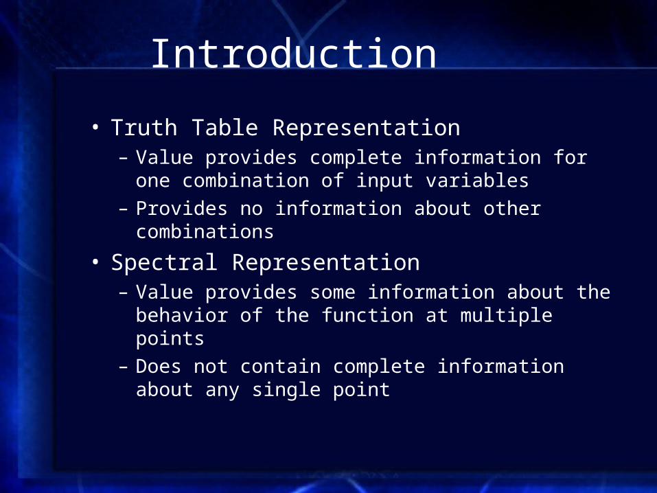
Review – Linear Algebra
• Let M be a real-valued square matrix.– The transposed matrix Mt is found by interchanging
rows and columns– M is orthogonal if
MMt = MtM = I
– M is orthogonal up to the constant k if MMt = MtM = kI
– M-1 is the inverse of M if MM-1 = M-1M = I
– M has its inverse iff the column vectors of M are linearly independent
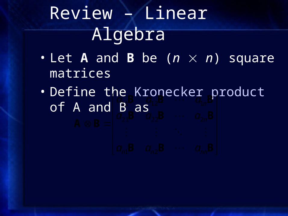
Review – Linear Algebra
• Let A and B be (n n) square matrices
• Define the Kronecker product of A and B as
BBB
BBB
BBB
BA
nnnn
n
n
aaa
aaa
aaa
21
22221
11211
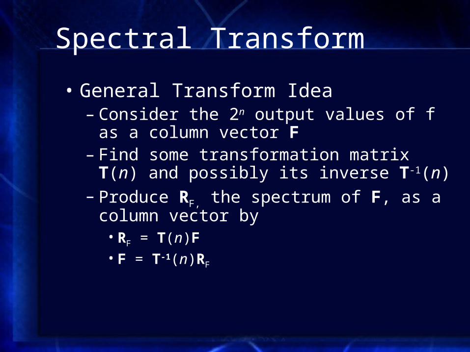
Spectral Transform
• General Transform Idea– Consider the 2n output values of f as a column
vector F– Find some transformation matrix T(n) and
possibly its inverse T-1(n)– Produce RF, the spectrum of F, as a column
vector by• RF = T(n)F• F = T-1(n)RF
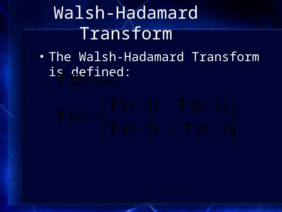
Walsh-Hadamard Transform
• The Walsh-Hadamard Transform is defined:
1)0( T
)1()1(
)1()1()(
nn
nnn
TT
TTT

Walsh-Hadamard Matrices
1111
1111
1111
1111
(2)
11
11)1(
T
Τ
11111111
11111111
11111111
11111111
11111111
11111111
11111111
11111111
(3)T

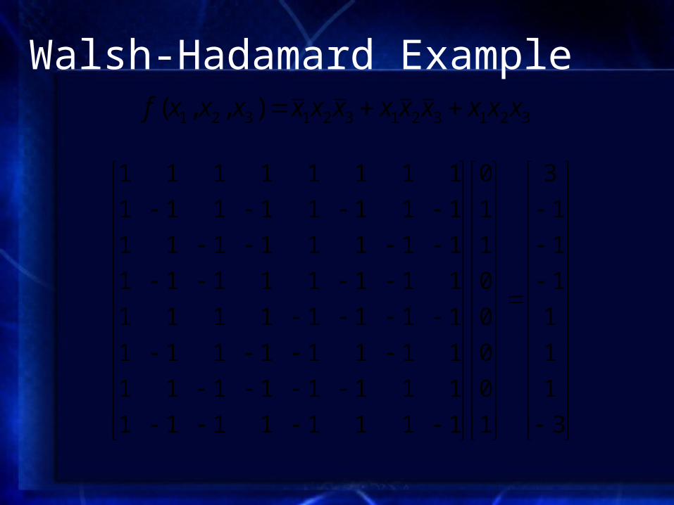
Walsh-Hadamard Example
1
0
0
0
0
1
1
0
11111111
11111111
11111111
11111111
11111111
11111111
11111111
11111111
321321321321 ),,( xxxxxxxxxxxxf

Walsh-Hadamard Example
1
0
0
0
0
1
1
0
11111111
11111111
11111111
11111111
11111111
11111111
11111111
11111111
321321321321 ),,( xxxxxxxxxxxxf
3
Walsh-Hadamard Example
3
1
1
1
1
1
1
3
1
0
0
0
0
1
1
0
11111111
11111111
11111111
11111111
11111111
11111111
11111111
11111111
321321321321 ),,( xxxxxxxxxxxxf

Walsh-Hadamard Example
6
1
1
1
2
2
2
2
1
1
1
1
1
1
1
1
11111111
11111111
11111111
11111111
11111111
11111111
11111111
11111111
321321321321 ),,( xxxxxxxxxxxxf
Walsh-Hadamard Transform
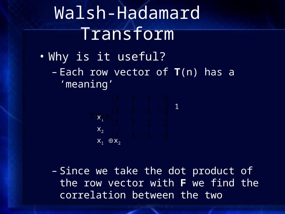
• Why is it useful?– Each row vector of T(n) has a ‘meaning’
1
x1
x2
x1 x2
– Since we take the dot product of the row vector with F we find the correlation between the two
1111
1111
1111
1111
(2)T
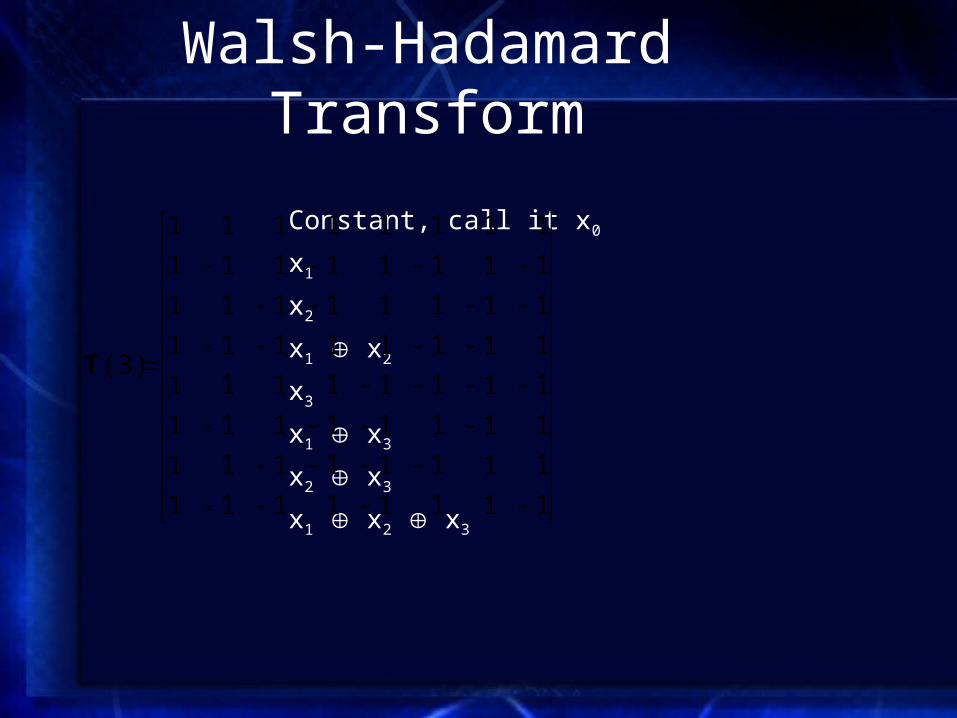
Walsh-Hadamard Transform
Constant, call it x0
x1
x2
x1 x2
x3
x1 x3
x2 x3
x1 x2 x3
11111111
11111111
11111111
11111111
11111111
11111111
11111111
11111111
(3)T
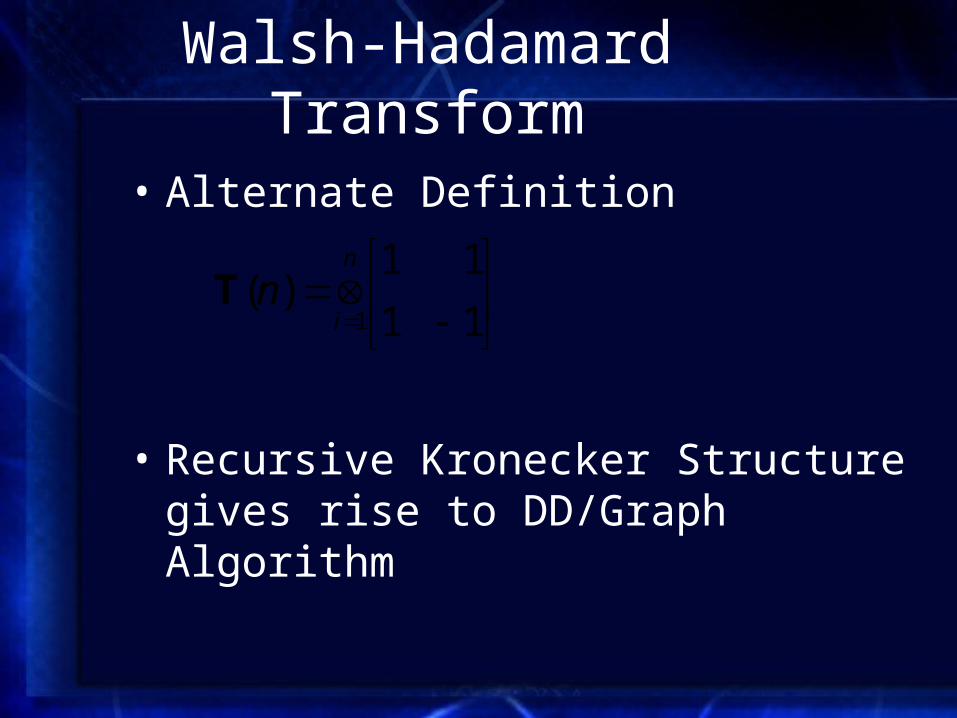
Walsh-Hadamard Transform
• Alternate Definition
• Recursive Kronecker Structure gives rise to DD/Graph Algorithm
11
11)(
1
n
inT
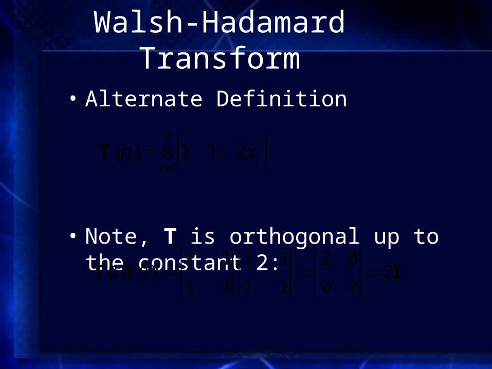
Walsh-Hadamard Transform
• Alternate Definition
• Note, T is orthogonal up to the constant 2:
in
ixn 211)(
1
T
IΤΤ 220
02
11
11
11
11)1()1(
t
Decision Diagrams
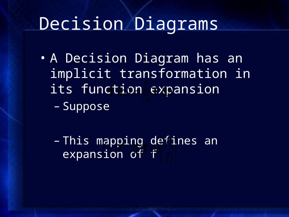
• A Decision Diagram has an implicit transformation in its function expansion– Suppose
– This mapping defines an expansion of f
)1()(1TT
n
in
1
01 )1()1(f
ff TT

Binary Decision Diagrams
• To understand this expansion better, consider the identity transformation
• Symbolically,
101
0
1
01 )1()1(
fxfxf
fxxf
f
ff
iiii
II
ii xxn
10
01)(T
Binary Decision Diagrams
• The expansion of f defines the node semantics
• By using the identity transform, we get standard BDDs
• What happens if we use the Walsh Transform?
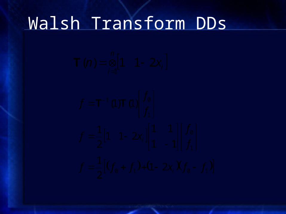
Walsh Transform DDs
in
ixn 211)(
1
T
1010
1
0
1
01
212
1
11
11211
2
1
)1()1(
ffxfff
f
fxf
f
ff
i
i
TT

Walsh Transform DDs
1010 212
1ffxfff i •
102
1ff 102
1ff
1 ix21
Walsh Transform DDs
• It is possible to convert a BDD into a WTDD via a graph traversal.
• The algorithm essentially does a DFS
Applications: Synthesis
• Several different approaches (all very promising) use spectral techniques– SPECTRE – Spectral Translation– Using Spectral Information as a heuristic– Iterative Synthesis based on Spectral
Transforms
Thornton’s Method
• M. Thornton developed an iterative technique for combination logic synthesis
• Technique is based on finding correlation with constituent functions
• Needs a more arbitrary transformation than Walsh-Hadamard– This is still possible quickly with DD’s

Thornton’s Method
• Constituent Functions– Boolean functions whose output vectors are the
rows of the transformation matrix– If we use XOR as the primitive, we get the
rows for the Walsh-Hadamard matrix• Other functions are also permissible
Thornton’s Method
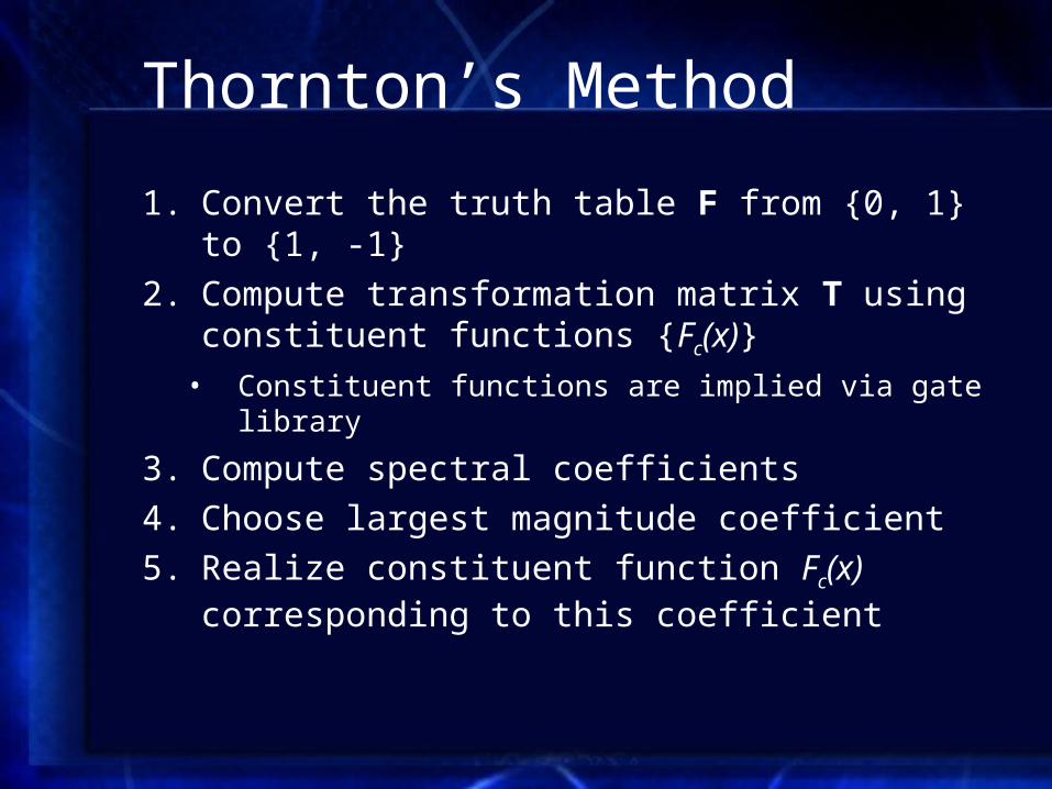
1. Convert the truth table F from {0, 1} to {1, -1}
2. Compute transformation matrix T using constituent functions {Fc(x)}
• Constituent functions are implied via gate library
3. Compute spectral coefficients
4. Choose largest magnitude coefficient
5. Realize constituent function Fc(x) corresponding to this coefficient
Thornton’s Method
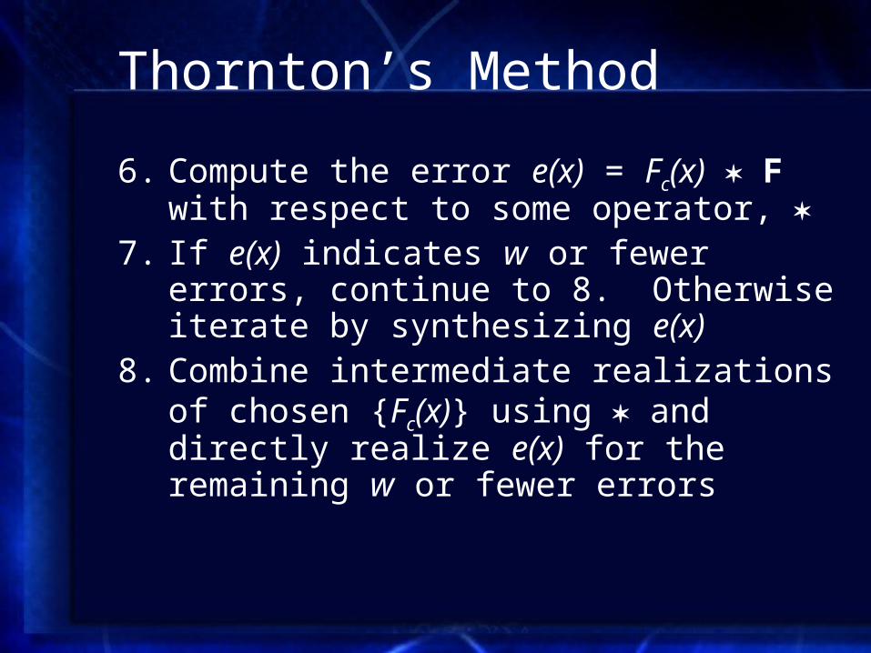
6. Compute the error e(x) = Fc(x) F with respect to some operator,
7. If e(x) indicates w or fewer errors, continue to 8. Otherwise iterate by synthesizing e(x)
8. Combine intermediate realizations of chosen {Fc(x)} using and directly realize e(x) for the remaining w or fewer errors
Thornton’s Method
• Guaranteed to converge
• Creates completely fan-out free circuits
• Essentially a repeated correlation analysis
• Extends easily to multiple gate libraries
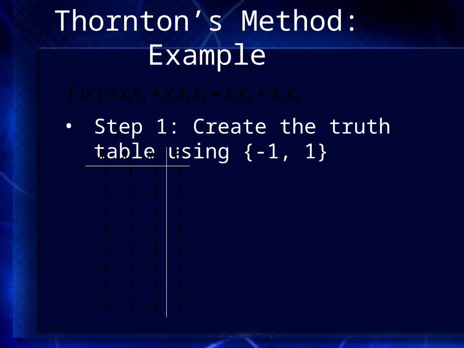
Thornton’s Method: Example
• Step 1: Create the truth table using {-1, 1}322132131)( xxxxxxxxxxf
1111
1111
1111
1111
1111
1111
1111
1111321
Fxxx

Thornton’s Method: Example
• Step 2: Compute transformation matrix T using constituent functions.
• In this case, we’ll use AND, OR, XOR

Thornton’s Method: Example
1
x1
x2
x3
x1 x2
x1 x3
x2 x3
x1 x2 x3
x1 + x2
x1 + x3
x2 + x3
x1 + x2 + x3
x1x2
x1x3
x2x3
x1x2x3
11111111
11111111
11111111
11111111
11111111
11111111
11111111
11111111
11111111
11111111
11111111
11111111
11111111
11111111
11111111
11111111

Thornton’s Method: Example
• Step 3: Compute spectral coefficients
• S[Fc(x)]= [-2, -2, 2, -2, 2, -2, 2, -6, 2,
-2, 2, 2, -2, -2, -2, -4]
• Step 4: Choose largest magnitude coefficient.– In this case, it corresponds to x1 x2 x3
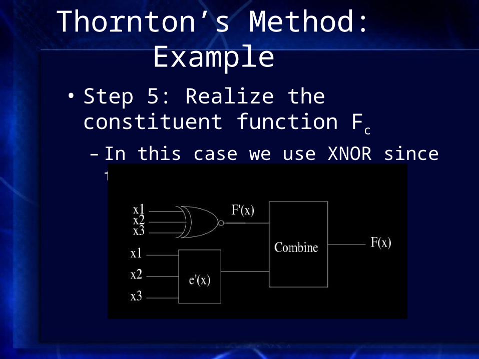
Thornton’s Method: Example
• Step 5: Realize the constituent function Fc
– In this case we use XNOR since the coefficient is negative

Thornton’s Method: Example
• Step 6: Compute the error function e(x)– Use XOR as a robust error operator
111111
111111
111111
111111
111111
111111
111111
111111321
eFxxx cF
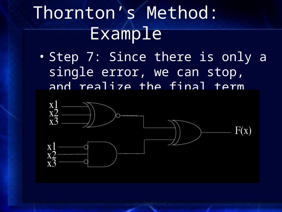
Thornton’s Method: Example
• Step 7: Since there is only a single error, we can stop, and realize the final term directly

Conclusion
• The combination of spectral transforms and implicit representation has many applications
• Many ways to leverage the spectral information for synthesis