2013-10-01 SGS 1

Fast Solar Polarimeter

Alex FellerFrancisco Iglesias

Nagaraju KrishnappaSami K. Solanki

2013-10-01 SGS 2

FSP in a nutshell

● Novel ground-based solar imaging polarimeter developed by MPS in collaboration with the MPG semiconductor lab and PNSensor corp.

● Funded by Max Planck society and European Commission (SOLARNET)

● Based on fast, low-noise pnCCD sensor and ferro-electric liquid crystals (FLCs) for polarization modulation

● Polarimetric sensitivity: 0.01%

● Targeted mainly at statistical studies of weak photospheric and chromospheric polarization signals at high spatial or temporal resolution

● Development in 2 phases:

– Phase I (2011-2013): proof of concept with small pnCCD prototype (264 x 264 pixels), single-beam setup

– Phase II (2014-2016): Full-scale, science-ready instrument with two 1k x 1k pnCCDs

2013-10-01 SGS 3

Main scientific focus of FSP● Study of

– ubiquitous small-scale magnetic processes in the quiet Sun photosphere and chromosphere

– radiative processes (scattering polarization) on smaller spatial scales

● The limited photon flux suggests a statistical approach to reach an increased polarimetric sensitivity by

– Feature classification in high-resolution Stokes images, spatially binning into classes of pixels (e.g. granules / intergranular lanes, cf. Snik et al. 2010)

– Feature tracking in time of highly dynamic structures, e.g. in the chromosphere Predicted small-scale scattering polarization

in Sr I 460.7 nm, based on MHD simulations (Trujillo Bueno & Shchukina 2007)

2013-10-01 SGS 4

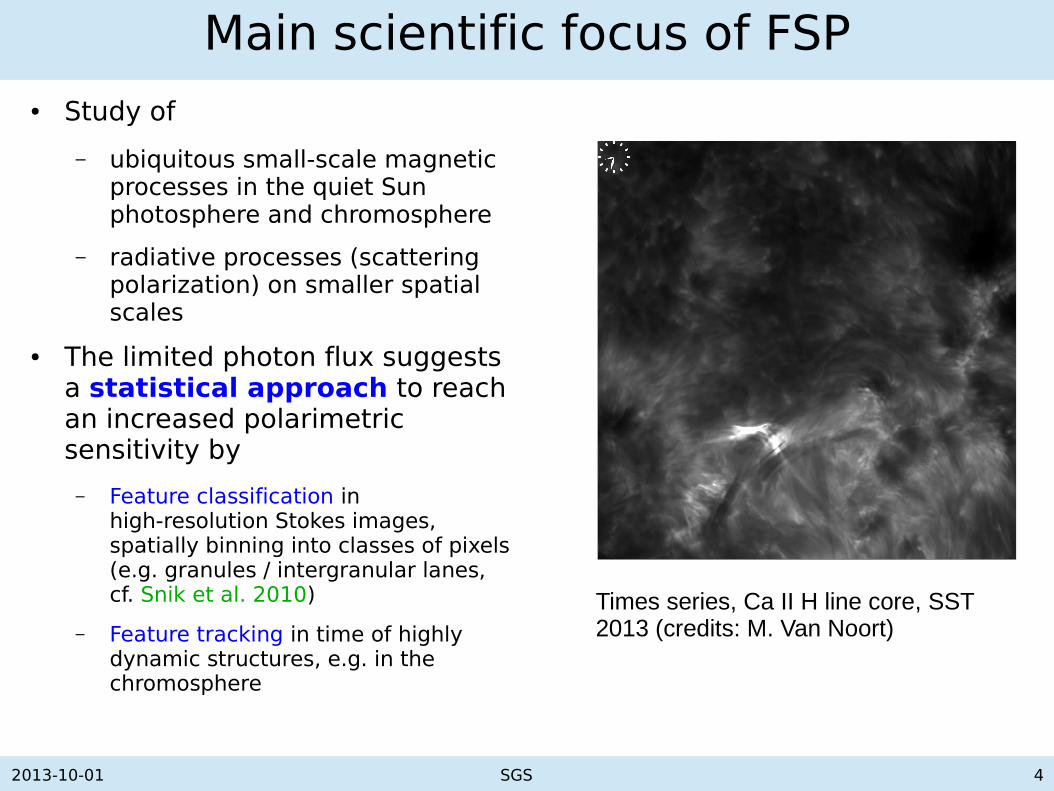
Main scientific focus of FSP

Times series, Ca II H line core, SST 2013 (credits: M. Van Noort)

● Study of

– ubiquitous small-scale magnetic processes in the quiet Sun photosphere and chromosphere

– radiative processes (scattering polarization) on smaller spatial scales

● The limited photon flux suggests a statistical approach to reach an increased polarimetric sensitivity by

– Feature classification in high-resolution Stokes images, spatially binning into classes of pixels (e.g. granules / intergranular lanes, cf. Snik et al. 2010)

– Feature tracking in time of highly dynamic structures, e.g. in the chromosphere

2013-10-01 SGS 5

Polarimetry basics

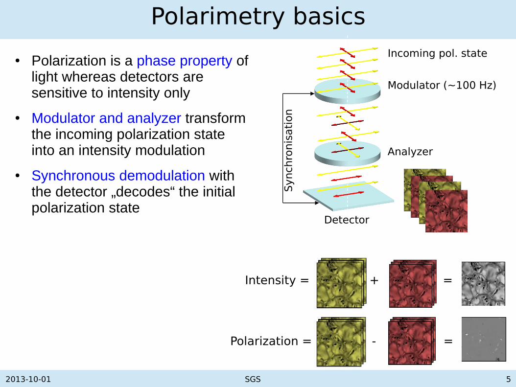
Intensity = + =

Polarization = - =

● Polarization is a phase property of light whereas detectors are sensitive to intensity only

● Modulator and analyzer transform the incoming polarization state into an intensity modulation

● Synchronous demodulation with the detector „decodes“ the initial polarization state

Incoming pol. state

Modulator (~100 Hz)

Analyzer

Detector

Synch

ronis

ati

on

2013-10-01 SGS 6

Why fast modulation?

● In order to detect a polarization signal of 0.01% we have to perform differential intensity measurements at the same level of precision

● Polarimetry is therefore very sensitive to instabilities during measurement, e.g.:

– Atmospheric turbulence

– Vibrations in the instrument

– Detector gain fluctuations

Top panels: Simulated measurement of Zeeman signals of the quiet Sun granulation in Fe I 630.2 nm with a random image jitter of 0.1 detector pixels rms.

Bottom panels: clean reference measurement without jitter.

See also Lites 1987, Judge et al. 2004, Casini et al. 2012.

2013-10-01 SGS 7

Polarimetry basics● Modulation matrix

I = M.S

S = (I, Q, U, V): incoming (solar) Stokes vector

I = (I1, …, In): measured intensities for the different modulator states

● Polarimetric accuracy

Smeas = Mmeas-1.M.S

Response matrix: R = Mmeas-1.M

Crosstalk: non-diagonal elements of R

● Polarimetric sensitivity

Smeas = Mmeas-1.I =: D.I

Efficiency: εi=σ Iσi

=(n∑j=1

n

Dij2 )

−1/2,i= I ,Q ,U ,V

2013-10-01 SGS 8

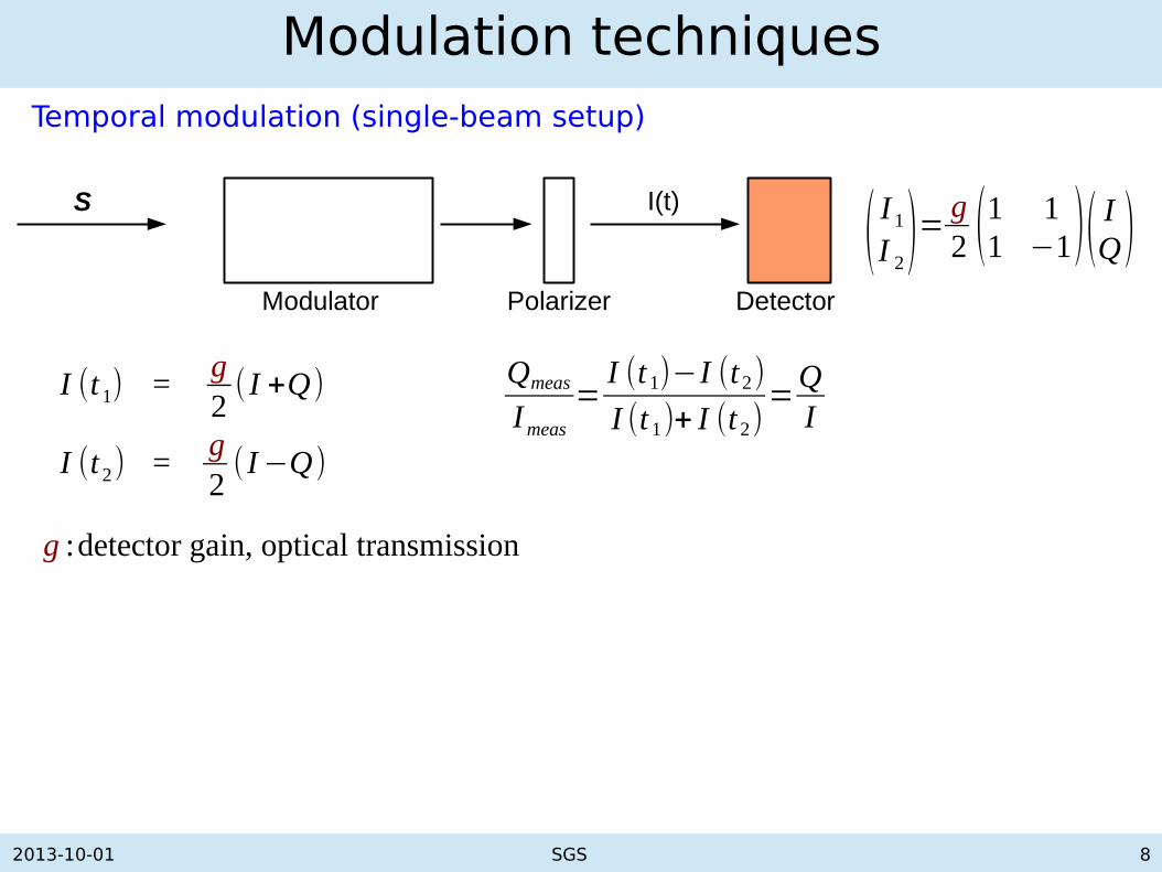
Modulation techniques

I (t 1) =g2

( I +Q)

I (t 2) =g2

( I−Q)

Qmeas

Imeas

=I (t 1)−I (t 2)

I (t 1)+ I (t 2)=

QI

( I 1

I 2)=

g2 (1 1

1 −1)( IQ)

Modulator Polarizer Detector

S I(t)

Temporal modulation (single-beam setup)

g :detector gain, optical transmission

2013-10-01 SGS 9

Modulation techniquesTemporal modulation (single-beam setup)

Modulator Polarizer Detector

S I(t)

I (t 1) =g2

(I +δ I 1+Q+δQ1)

I (t 2) =g2

(I +δ I 2−Q−δQ2)

δ I ≈ ∇ I δ r ,δQ ≈ ∇Q δ r

Qmeas

Imeas

=I 1− I 2

I 1+ I 2

=Q+

12(δQ1+δQ 2)+

12(δ I 1−δ I 2)

I+12(δ I 1+δ I 2)+

12(δQ1−δQ2)

With disturbances δQ ,δ I , for example from jitter δ r :

In practice, for slow modulation :δ II

≈δQQ

≈10−2 ... 10−1

2013-10-01 SGS 10

Modulation techniquesTemporal modulation (single-beam setup)

Modulator Polarizer Detector

S I(t)

I (t 1) =g2

(I +δ I 1+Q+δQ1)

I (t 2) =g2

(I +δ I 2−Q−δQ2)

δ I ≈ ∇ I δ r ,δQ ≈ ∇Q δ r

Qmeas

Imeas

=I 1− I 2

I 1+ I 2

=Q+

12(δQ1+δQ 2)+

12(δ I 1−δ I 2)

I+12(δ I 1+δ I 2)+

12(δQ1−δQ2)

With disturbances δQ ,δ I , for example from jitter δ r :

In practice, for slow modulation :δ II

≈δQQ

≈10−2 ... 10−1

Polar. error

Spatial „smearing“

2013-10-01 SGS 11

Modulation techniquesSpatial modulation (dual-beam setup)

Modulator Detector 1

S I1

Detector 2

I2

Pol. beamsplitter

I 1 =g2

( I+δ I +Q+δQ)

I 2 =g+δ g

2(I +δ I−Q−δQ)

Qmeas

Imeas

=I 1−I 2

I 1+ I 2

=(g +

δ g2 )(Q+δQ)−

δ g2

( I+δ I )

(g +δ g2 )(I +δ I )−

δ g2

(Q+δQ)

δgg≈10−3

Differential detector gain or opt. transmission:

2013-10-01 SGS 12

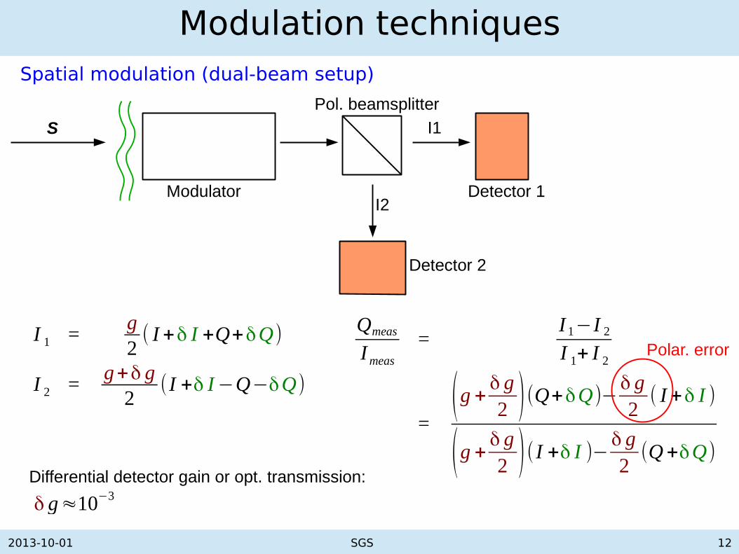
Modulation techniquesSpatial modulation (dual-beam setup)

Modulator Detector 1

S I1

Detector 2

I2

Pol. beamsplitter

I 1 =g2

( I+δ I +Q+δQ)

I 2 =g+δ g

2(I +δ I−Q−δQ)

Qmeas

Imeas

=I 1−I 2

I 1+ I 2

=(g +

δ g2 )(Q+δQ)−

δ g2

( I+δ I )

(g +δ g2 )(I +δ I )−

δ g2

(Q+δQ)

δ g≈10−3

Differential detector gain or opt. transmission:

Polar. error

2013-10-01 SGS 13

Modulation techniquesMixed spatial and temporal modulation (e.g. Semel et al. 1993)

Modulator Detector 1

S I1(t)

Detector 2

I2(t)

Pol. beamsplitter

I 1(t 1) =g2

( I+δ I 1+Q+δQ 1)

I 2( t1) =g+δ g

2(I +δ I 1−Q−δQ1)

I 1(t 2) =g2

( I+δ I 2−Q−δQ2)

I 2(t 2) =g+δ g

2(I +δ I 2+Q+δQ 2)

Qmeas

Imeas

=I 1( t1)− I 1(t 2)− I 2(t 1)+ I 2(t 2)

I 1(t 1)+ I 1(t 2)+ I 2( t1)+ I 2(t 2)

=(g +

δ g2 )(Q+

δQ 1+δQ2

2 )+ δ g4

(δ I 2−δ I 1)

(g+δ g2 )( I +

δ I 1+δ I 2

2 )+ δ g4

(δQ 2−δQ1)

2013-10-01 SGS 14

Modulation techniquesMixed spatial and temporal modulation (e.g. Semel et al. 1993)

Modulator Detector 1

S I1(t)

Detector 2

I2(t)

Pol. beamsplitter

I 1(t 1) =g2

( I+δ I 1+Q+δQ 1)

I 2( t1) =g+δ g

2(I +δ I 1−Q−δQ1)

I 1(t 2) =g2

( I+δ I 2−Q−δQ2)

I 2(t 2) =g+δ g

2(I +δ I 2+Q+δQ 2)

Qmeas

Imeas

=I 1( t1)− I 1(t 2)− I 2(t 1)+ I 2(t 2)

I 1(t 1)+ I 1(t 2)+ I 2( t1)+ I 2(t 2)

=(g +

δ g2 )(Q+

δQ 1+δQ2

2 )+ δ g4

(δ I 2−δ I 1)

(g+δ g2 )( I +

δ I 1+δ I 2

2 )+ δ g4

(δQ 2−δQ1)

Spatial „smearing“

2013-10-01 SGS 15

Why fast modulation?Simulated seeing induced crosstalk as a function of AO correction and modulation frequency for a single-beam setup (Nagaraju & Feller, Appl. Opt., 2012).

2013-10-01 SGS 16

Why fast modulation?Simulated seeing induced crosstalk as a function of AO correction and modulation frequency for a dual-beam setup (Nagaraju & Feller, Appl. Opt., 2012).

2013-10-01 SGS 17

Why fast modulation?

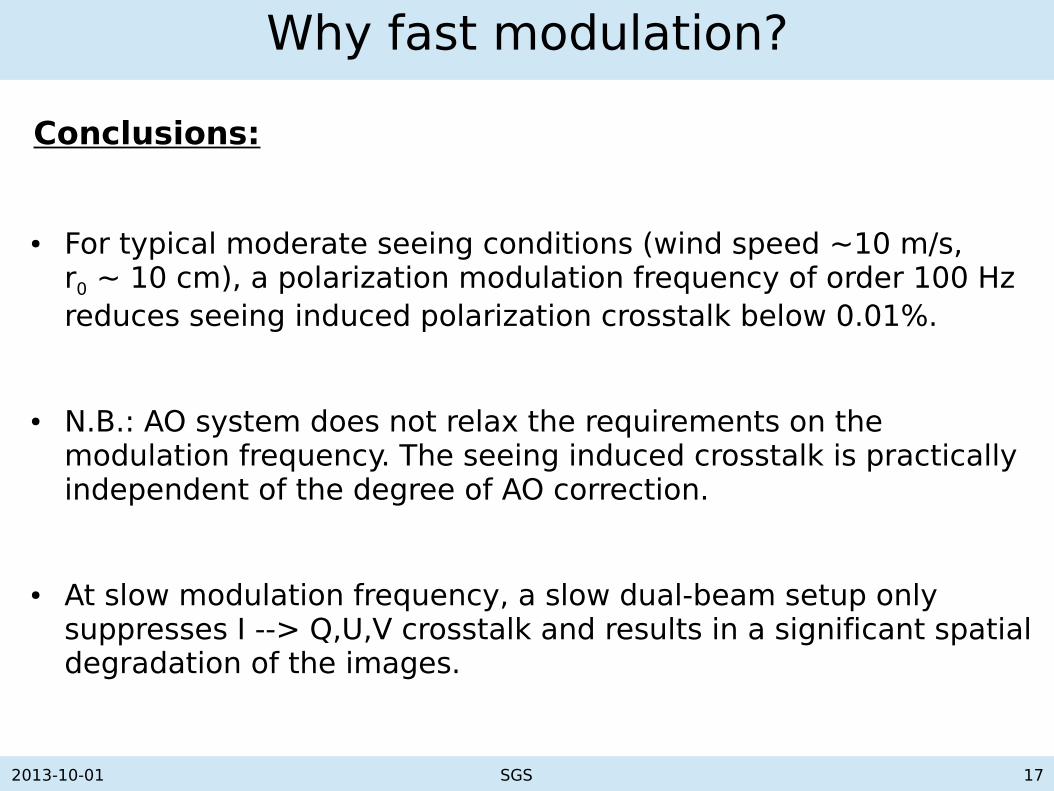
Conclusions:

● For typical moderate seeing conditions (wind speed ~10 m/s, r0 ~ 10 cm), a polarization modulation frequency of order 100 Hz reduces seeing induced polarization crosstalk below 0.01%.

● N.B.: AO system does not relax the requirements on the modulation frequency. The seeing induced crosstalk is practically independent of the degree of AO correction.

● At slow modulation frequency, a slow dual-beam setup only suppresses I --> Q,U,V crosstalk and results in a significant spatial degradation of the images.

2013-10-01 SGS 18

FSP first-light campaign

● First test of the prototype instrument at the German VTT on Tenerife in June 2013

● Spectrograph mode, low spatial resolution (0.2 - 0.4 arcsec/pixel)

● Focus on functional and performance tests

– at different modulation frequencies

– under different atmospheric seeing conditions

● Measurements

– Zeeman diagnostics in Fe I lines (525.0 nm, 630.2 nm), Sunrise II co-observations

– Scattering polarization at the solar limb (Ca I 422.7 nm, Sr I 460.7 nm)

2013-10-01 SGS 19

FSP first-light campaign: setup

FSP modulator, mounted on top of the spectrograph entrance slit

FSP camera with re-imaging optics, mounted at a spectrograph exit port

2013-10-01 SGS 20

Some test results

Scan of active region (NOAA 11762) in Fe I 525 nm

Greyscales: 0.2-1.3 <I>, ± 0.2 for Q/I, U/I, V/I

2013-10-01 SGS 21

Some test results

Scattering polarization in Ca I 422.7 nm at µ = 0.15

2013-10-01 SGS 22

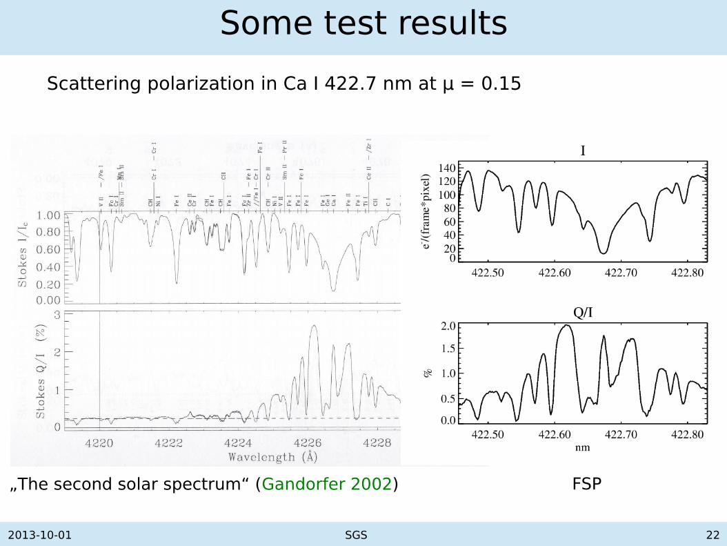
Some test results

Scattering polarization in Ca I 422.7 nm at µ = 0.15

„The second solar spectrum“ (Gandorfer 2002) FSP

2013-10-01 SGS 23

Some test results

Scattering polarization in Sr I 460.7 nm at µ = 0.15

2013-10-01 SGS 24

Photon budgetAssumptions:

● Diffraction limited critical sampling (~ 12 pixels for PSF core)

● Throughput: 10%

● Exposure time: 2.5 ms (400 fps)

● Spectral sampling: 15 mÅ / pixel

● Polarimetric efficiency: 0.5

Example Ca II K 393 nm Fe I 525 nm Ca II 854.2 nm

Intensity phot / (s · m2 · nm · sterad)

1.5 · 1021

2 · 1022 1.3 · 1022

Flux per pixel and frame 25 e- 300 e- 200 e-

No. of pixels to average for 0.01% polarimetric sensitivity, after 1s integration

40'000(4% of detector area)

3300 5000

2013-10-01 SGS 26

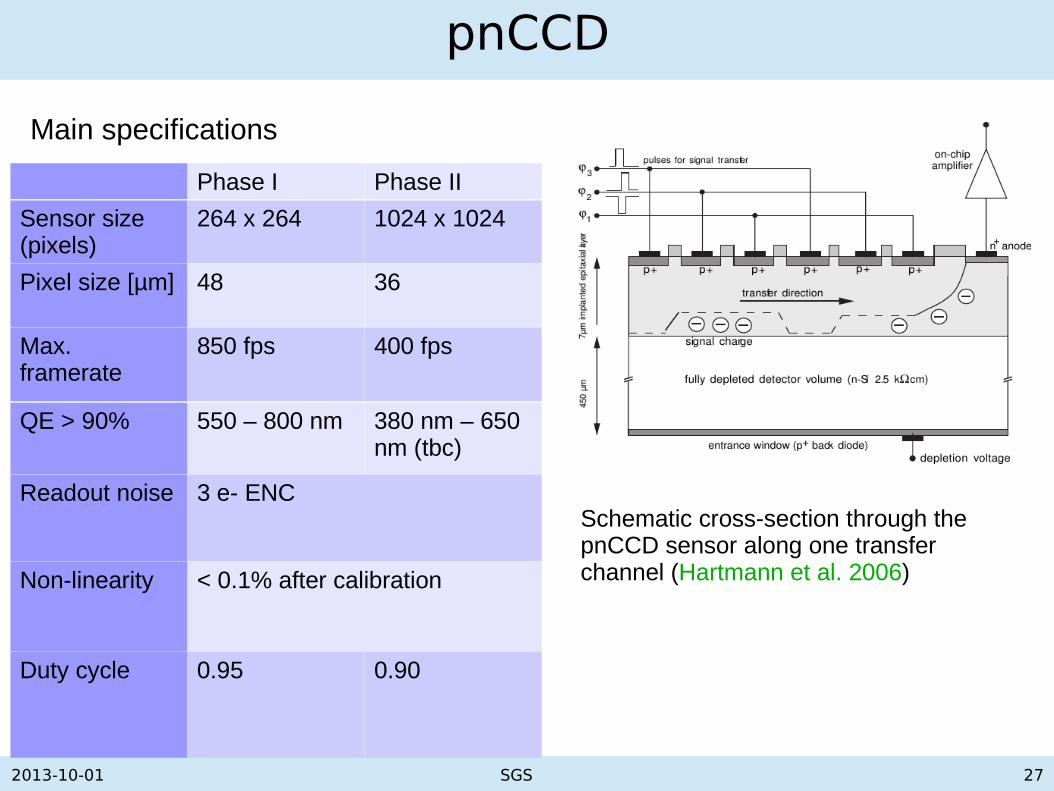
pnCCD

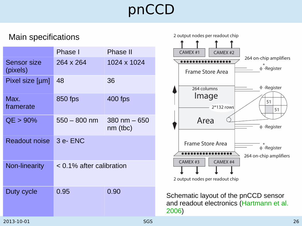
Phase I Phase II

Sensor size (pixels)

264 x 264 1024 x 1024

Pixel size [µm] 48 36

Max. framerate

850 fps 400 fps

QE > 90% 550 – 800 nm 380 nm – 650 nm (tbc)

Readout noise 3 e- ENC

Non-linearity < 0.1% after calibration

Duty cycle 0.95 0.90

Main specifications

Schematic layout of the pnCCD sensor and readout electronics (Hartmann et al. 2006)

2013-10-01 SGS 27

pnCCD

Main specifications

Schematic cross-section through the pnCCD sensor along one transfer channel (Hartmann et al. 2006)

Phase I Phase II

Sensor size (pixels)

264 x 264 1024 x 1024

Pixel size [µm] 48 36

Max. framerate

850 fps 400 fps

QE > 90% 550 – 800 nm 380 nm – 650 nm (tbc)

Readout noise 3 e- ENC

Non-linearity < 0.1% after calibration

Duty cycle 0.95 0.90

2013-10-01 SGS 28

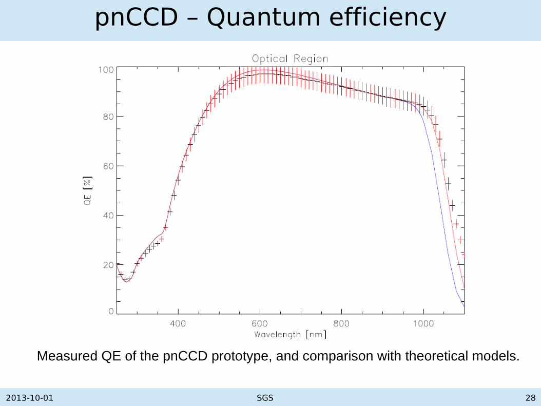
pnCCD – Quantum efficiency

Measured QE of the pnCCD prototype, and comparison with theoretical models.

2013-10-01 SGS 29

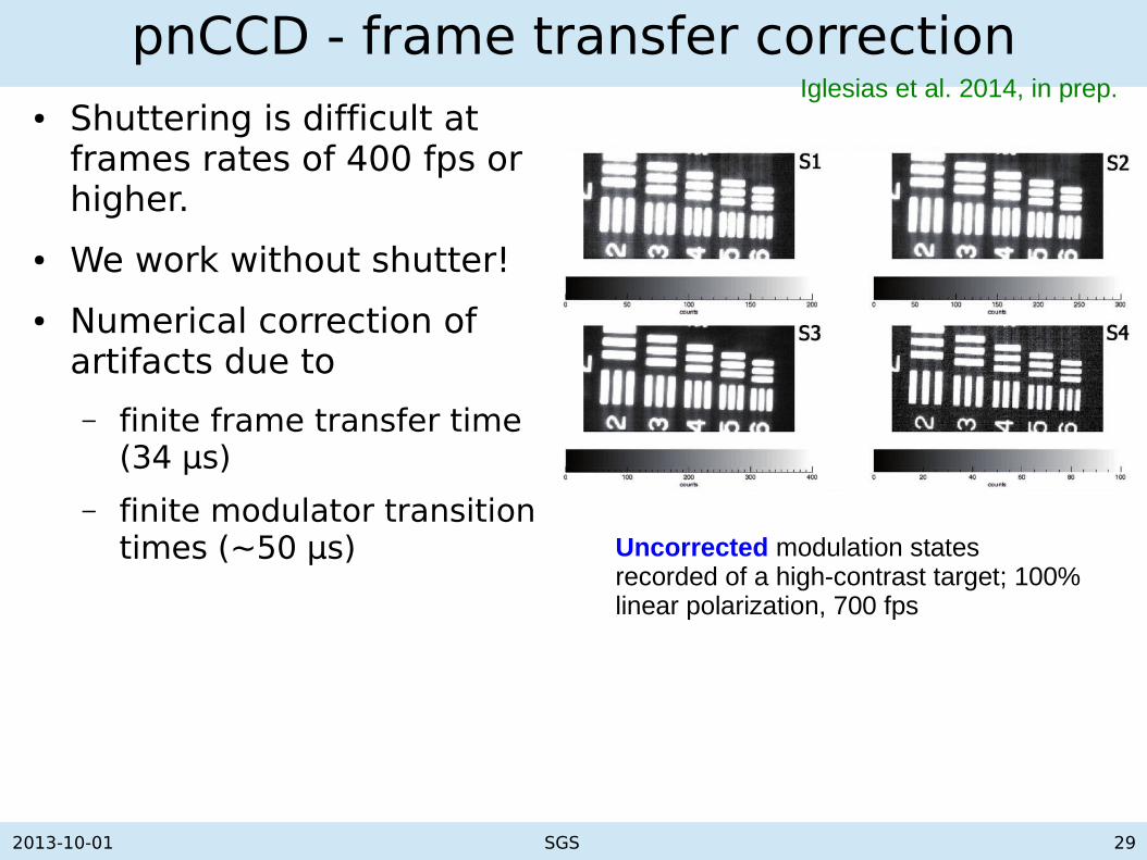
pnCCD - frame transfer correction● Shuttering is difficult at

frames rates of 400 fps or higher.

● We work without shutter!

● Numerical correction of artifacts due to

– finite frame transfer time (34 µs)

– finite modulator transition times (~50 µs) Uncorrected modulation states

recorded of a high-contrast target; 100% linear polarization, 700 fps

Iglesias et al. 2014, in prep.

2013-10-01 SGS 30

pnCCD - frame transfer correction● Shuttering is difficult at

frames rates of 400 fps or higher.

● We work without shutter!

● Numerical correction of artifacts due to

– finite frame transfer time (34 µs)

– finite modulator transition times (~50 µs) Same measurement after frame

transfer correction.

Iglesias et al. 2014, in prep.

2013-10-01 SGS 31

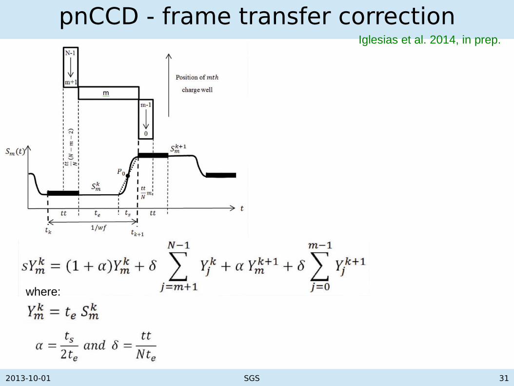
pnCCD - frame transfer correction

where:

Iglesias et al. 2014, in prep.

2013-10-01 SGS 32

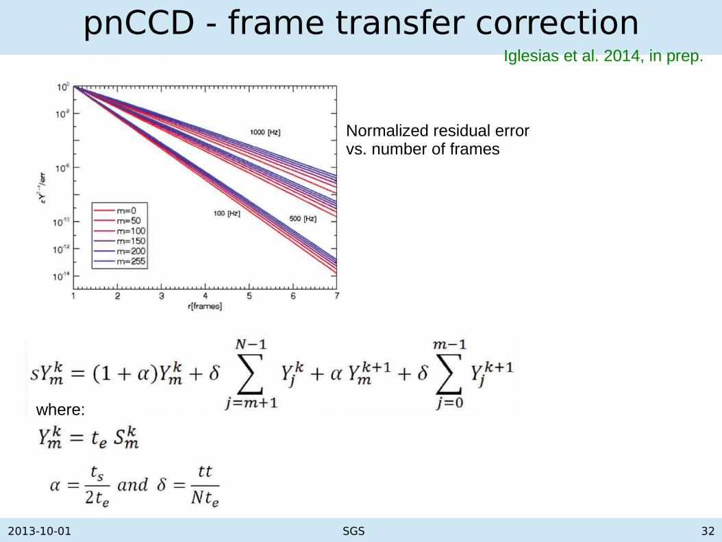
pnCCD - frame transfer correction

where:

Normalized residual error vs. number of frames

Iglesias et al. 2014, in prep.

2013-10-01 SGS 33

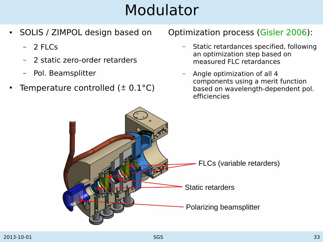
Modulator● SOLIS / ZIMPOL design based on

– 2 FLCs

– 2 static zero-order retarders

– Pol. Beamsplitter

● Temperature controlled (± 0.1°C)

Optimization process (Gisler 2006):

– Static retardances specified, following an optimization step based on measured FLC retardances

– Angle optimization of all 4 components using a merit function based on wavelength-dependent pol. efficiencies

FLCs (variable retarders)

Static retarders

Polarizing beamsplitter

2013-10-01 SGS 34

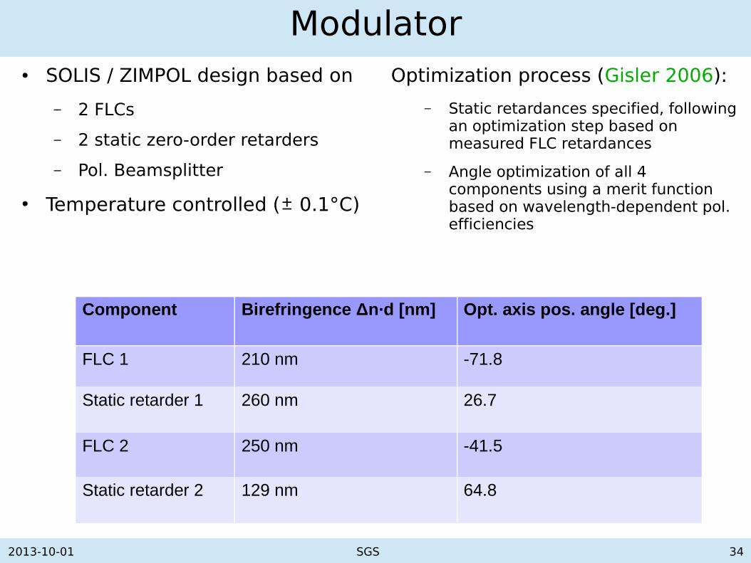
Modulator

Component Birefringence Δn·d [nm] Opt. axis pos. angle [deg.]

FLC 1 210 nm -71.8

Static retarder 1 260 nm 26.7

FLC 2 250 nm -41.5

Static retarder 2 129 nm 64.8

● SOLIS / ZIMPOL design based on

– 2 FLCs

– 2 static zero-order retarders

– Pol. Beamsplitter

● Temperature controlled (± 0.1°C)

Optimization process (Gisler 2006):

– Static retardances specified, following an optimization step based on measured FLC retardances

– Angle optimization of all 4 components using a merit function based on wavelength-dependent pol. efficiencies

2013-10-01 SGS 35

FSP performance

Pol. efficiency at 630 nm vs. modulation frequency

Mod. frequency [Hz]

Pol. efficiency at 25 Hz vs. wavelength

Mod. frequency [Hz]

Wavelength [nm]

2013-10-01 SGS 37

FSP performance

Analysis of pol. efficiency with modulator switched off (Fe I 630.2 nm)

Mod. freq. [Hz] Quiet Sun Pore region

25

50

100

Nagaraju et al. 2014, in prep.

2013-10-01 SGS 39

Lessons learned so far ...

● The small FSP prototype has performed reliably at the VTT during its first-light campaign in June.

● Shutterless operation with post-facto frame transfer correction works sufficiently well. Room for improvement taking into account the finite FLC response.

● Polarimetric efficiency close to theoretical expectations. Stable response in time thus requiring less frequent calibration.

● A frame rate of order 400 fps (modulation frequency 100 Hz) is crucial for observing high contrast targets on the Sun at 0.01% noise level.

● Polarimetric sensitivity of 0.01% - 0.02% is currently reached.

● However, at a noise level below 0.1% we see some artifacts, related to modulator and camera, which need further analysis.

● Telescope polarization compensation needed!

2013-10-01 SGS 40

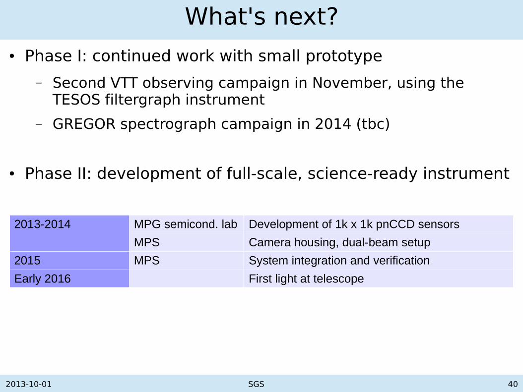
What's next?● Phase I: continued work with small prototype

– Second VTT observing campaign in November, using the TESOS filtergraph instrument

– GREGOR spectrograph campaign in 2014 (tbc)

● Phase II: development of full-scale, science-ready instrument

2013-2014 MPG semicond. lab Development of 1k x 1k pnCCD sensors

MPS Camera housing, dual-beam setup

2015 MPS System integration and verification

Early 2016 First light at telescope