Fast parallel solver for the levelset equations on …kirby/Publications/Kirby-90.pdfFast parallel solver for the levelset equations on unstructured meshes Zhisong Fu*, †, Sergey

CONCURRENCY AND COMPUTATION: PRACTICE AND EXPERIENCEConcurrency Computat.: Pract. Exper. 2015; 27:1639–1657Published online 4 July 2014 in Wiley Online Library (wileyonlinelibrary.com). DOI: 10.1002/cpe.3320

Fast parallel solver for the levelset equations onunstructured meshes

Zhisong Fu*,†, Sergey Yakovlev, Robert M. Kirby and Ross T. Whitaker

Scientific Computing and Imaging Institute, University of Utah, Salt Lake City, UT, USA

SUMMARY

The levelset method is a numerical technique that tracks the evolution of curves and surfaces governedby a nonlinear partial differential equation (levelset equation). It has applications within various researchareas such as physics, chemistry, fluid mechanics, computer vision, and microchip fabrication. Applyingthe levelset method entails solving a set of nonlinear partial differential equations. This paper presents aparallel algorithm for solving the levelset equations on unstructured 2D and 3D meshes. By taking intoaccount constraints and capabilities of different computing architectures, the method is suitable for boththe coarse-grained parallelism found on CPU-based systems and the fine-grained parallelism of modernmassively single instruction, multiple data architectures such as graphics processors. In order to solve thelevelset equations efficiently, we combine the narrowband scheme with a domain decomposition that isadapted for several different architectures. We also introduce a novel parallelism strategy, which we callhybrid gathering, which allows regular and lock-free computations of local differential operators. Finally,we provide the detailed description of the implementation and data structures for the proposed strategies, aswell as performance data for both CPU and graphics processing unit implementations. Copyright © 2014John Wiley & Sons, Ltd.

Received 12 June 2013; Revised 8 April 2014; Accepted 29 May 2014

KEY WORDS: levelset equations; unstructured meshes; parallel computing; graphics processing unit

1. INTRODUCTION

The levelset method uses a scalar function � D �.x.t/; t/ to implicitly represent a surface or a curve,S D ¹x.t/ j �.x.t// D kº, hereafter referenced as a surface. The surface evolution is capturedby numerically solving the associated nonlinear partial differential equation (levelset equation).The levelset method has a wide array of application areas, ranging from geometry, fluid mechan-ics, and computer vision to manufacturing processes [1] and, virtually, any problem that requiresinterface tracking. The method was originally proposed for regular grids by Osher and Sethian [2],and the early levelset implementations used finite difference approximations on fixed, logically rec-tilinear grids. Such techniques have the advantages of a high degree of accuracy and programmingease. However, in some situations, a triangulated domain with finite element-type approximationsis desired. Barth and Sethian have cast the levelset method into the finite element frameworkand extended it to unstructured meshes in [3]. Since then, the levelset method has been widelyused in applications that involve complex geometry and require the use of unstructured meshes forsimulation. For example, in medical imaging, the levelset method on a brain surface is used forautomatic sulcal delineation, which is important for investigating brain development and diseasetreatment [4]. In computer graphics, researchers have been using levelset methods for featuredetection and mesh subdivision via geodesic curvature flow [5]. Yet another application of

*Correspondence to: Zhisong Fu, Scientific Computing and Imaging Institute, University of Utah, Salt Lake City, UT,USA

†E-mail: [email protected]

Copyright © 2014 John Wiley & Sons, Ltd.

1640 Z. FU ET AL.

the levelset method on unstructured domains is the simulation of solidification and crystal growthprocesses [6].

Many studies have been conducted to develop efficient levelset solvers. In [7], Adalsteinsson andSethian propose a narrowband scheme to speed up the computation. This approach is based on theobservation that one is typically only interested in a particular interface, in which case, the levelsetequation only needs to be solved in a band around the interface. Whitaker proposes the sparse fieldmethod in [8], which employs the narrowband concept and maintains a narrowband containing onlythe wavefront nodes and their neighbors to further improve the performance. We should also pointto several works that focus on the memory efficiency of the levelset method. Bridson proposes thesparse block grid method in [9] to dynamically allocate and free memory and achieves suboptimalstorage complexity. Strain [10] proposes the octree levelset method that is also efficient in terms ofstorage. Houston et al. [11] apply the run-length encoding scheme to compress regions away fromthe narrowband to adjust their sign representation while storing the narrowband with full precision,which further improves the storage efficiency over the octree approach. A number of recent works[12–17] address parallelism strategies for solving the levelset equations on CPU-based and graphicsprocessing unit (GPU)-based parallel systems. However, these works have been focused on regulargrids or coarse-grained parallel systems, and the parallelism schemes proposed do not readily extendto unstructured meshes and fine-grained parallel systems.

Recently, there has been growing interest in floating-point accelerators. These accelerators aredevices that perform arithmetic operations concurrently with or in place of the CPU. Two solutionshave received special attention from the high-performance computing community: GPUs, originallydeveloped to render graphics, which are now used for very demanding computational tasks, and thenewly released Intel Xeon Phi, which employs very wide (512 bit) single instruction, multiple data(SIMD) vectors on the same X86 architecture as other Intel CPUs and promises high performanceand little programming difficulty. Relative to CPUs, the faster growth curves of these acceleratorsin the speed and power efficiency have spawned a new area of development in computational tech-nology. Now, many of the top supercomputers, such as Titan, the current top one [18], are equippedwith such accelerators. Developing efficient code for these accelerators is a very important steptoward fully utilizing the power of such supercomputers. In this paper, we present efficient paral-lel algorithms for solving the levelset equations on unstructured meshes on both CPU-based andGPU-based parallel processing systems.

The use of unstructured meshes makes the levelset method more flexible with respect to compu-tational domains. However, solving the levelset equation on an unstructured mesh poses a numberof challenges for efficient parallel computing. First, there is no natural partition of the domainfor parallelism, and the use of a graph partitioner to decompose the mesh may result in unevenpartition sizes, which in turn leads to a load balancing problem. Second, for regular meshes, thevalence of the nodes is the same throughout the mesh, and hence, nodal parallelism (assigning eachnode to a thread) is typically employed. However, for unstructured meshes, the nodes have varyingvalence and local geometric structure, which leads to irregular data structures and unbalanced work-load for nodal parallelism. Third, the inter-partition communication typically requires additionalcomputation and separate data structures to find and store the partition boundary.

In this paper, we present a new parallelism strategy for solving the levelset equation on unstruc-tured meshes that combines the narrowband scheme and a domain decomposition. We propose thenarrowband fast iterative method (nbFIM) to compute the distance transform by solving the eikonalequation in a narrowband around the wavefront and the patched narrowband scheme (patchNB) toevolve the levelset. We use a unified domain partitioning for both distance transform and levelsetevolution to ensure minimal setup time. For unstructured meshes, the update of the value oneach node depends on values of its neighboring nodes, and a variable node valence may lead toload balancing issues. This is especially noticeable for GPUs and other streaming architectures,which employ SIMD-like architecture and prefer regular computations. To address this, we proposeelemental parallelism instead of nodal parallelism to mitigate load balancing problems. However,the elemental parallelism approach may result in race conditions, because multiple elements maytry to update the value of the same node simultaneously. Atomic operations are typically used tosolve this problem. However, atomic operations are expensive, especially on GPUs, and can result

Copyright © 2014 John Wiley & Sons, Ltd. Concurrency Computat.: Pract. Exper. 2015; 27:1639–1657DOI: 10.1002/cpe

FAST PARALLEL LEVELSET ON UNSTRUCTURED MESHES 1641

in significant numbers of threads blocking while waiting for access to variables. Therefore, we pro-pose a new lock-free algorithm (and associated data structures) to enforce data compactness andlocality for both shared memory CPU systems and GPUs. We call this approach hybrid gathering.Our algorithm converts the race condition problem to a sorting problem that is efficient on parallelsystems, including GPUs [19]. Both the distance transform (part of maintaining the narrowband)and the levelset evolution benefit from this lock-free update scheme. In this paper, we describe thedata structures and algorithms and present experimental results that demonstrate the efficiency ofthe proposed method on both shared memory CPU systems and GPUs.

The paper proceeds as follows. In Section 2, we introduce the levelset equation and the proposedmethod. In Section 3, we discuss implementation details and data structures. In Section 4, we discussthe performance of both CPU and GPU implementations of the proposed method, using several 2Dand 3D examples to measure performance. In Section 5, we summarize the results and discuss futureresearch directions related to this work.

2. MATHEMATICAL AND ALGORITHMIC DESCRIPTION

In general, the levelset equation solver with the narrowband scheme has two main building blocks:the distance transform recomputation (reinitialization) and the interface evolution according to thelevelset equation (evolution). In this section, we give the mathematical and algorithmic descriptionof the levelset method. We first introduce necessary notations and definitions and then describe thenarrowband scheme and the associated reinitialization algorithm. Finally, we present the numericalscheme for the evolution step and the novel hybrid gathering parallelism scheme and lock-freeupdate algorithm.

2.1. Notation and definitions

The levelset method relies on an implicit representation of a surface by a scalar function

� W �.x/! R; (1)

where � 2 Rd ; d 2 ¹2; 3º is the domain of the surface model, which can be a 2D plane, a 3Dvolume, or a manifold. Thus, a surface S is

S D ¹x j �.x/ D kº: (2)

The choice of k depends on the problem at hand, and we call � the embedding. The surface S isreferred to as an isosurface of �. Surfaces defined in this way partition � into inside and outsideparts, and such surfaces are always closed provided that they do not intersect the boundary of thedomain. The embedding � is approximated on a tessellation of the domain. The levelset methoduses a one-parameter family of embeddings, that is, �.x; t / changes over time t with x remainingon the k levelset of � as it moves and k remaining constant. The behavior of � is obtained by settingthe total derivative of �.x.t/; t/ D k to zero. Thus,

�.x.t/; t/ D k H)@�

@tCr� � v D 0: (3)

Let F denote the normal speed, F D v � r�j�j

. The levelset equation can then be written as

@�

@tC Fjr�j D 0: (4)

In general, F can be a more complicated function of x and rx, F D F.x;r�;r2�; : : :/. In thispaper, we consider the levelset equation with the normal speed function F of the following form:

F D ˛.x/ � r� C �.x/jr�j C ˇ.x/r �r�

jr�jjr�j; (5)


1642 Z. FU ET AL.

where ˛.x/, �.x/, and ˇ.x/ are user-defined coefficient functions. We call these three terms of Fthe advection term, the eikonal term, and the curvature term, respectively. This form of a levelsetequation is used widely in many applications such as image processing and computer vision.

We approximate the domain� by a tessellation�T , which consists of non-overlapping simplicesthat we call elements. Based upon this tessellation, we form a piecewise linear approximation of thesolution by maintaining the values of the approximation on the set of vertices V of the tessellationand employing linear interpolation within each element in �T . The total number of vertices in Vis denoted jV j, and the total number of elements in �T is denoted j�T j. We use vi to denote thei th vertex in V . An edge is a line segment connecting two vertices (vi , vj ) in Rd ; d 2 ¹2; 3º and isdenoted by eij . The vector from vertex vi to vertex vj is denoted by ei;j D xj � xi .

In this paper, we consider both 2D and 3D cases, and �T consists of triangles or tetrahedrarespectively. A triangle, denoted Tijk , is a set of three vertices vi , vj , vk that are pairwise connectedby an edge. Similarly, a tetrahedron is denoted Tijkl . The set of vertices adjacent to vertex vi iscalled one-ring neighbors of vi and is denoted by Ni , while the set of adjacent elements is calledone-ring elements of vi and is denoted by Ai . We denote the discrete approximation of the solution� at vertex vi by �i . The area or volume of an element T is denoted meas.T /.

2.2. Narrowband scheme and distance transform recomputation

Many applications require only a single surface model. In these cases, solving the levelset equationover the whole domain for every time-step is unnecessary and computationally inefficient. Fortu-nately, levelsets evolve independently (to within the error introduced by the discrete triangulation)and are not affected by the choice of embedding. Furthermore, the evolution of � is important onlyin the vicinity of that levelset. Thus, one should perform calculations for the evolution of � only ina neighborhood of the surface expressed by Equation 2. In the discrete setting, there is a particularsubset of mesh nodes whose values define a particular levelset. Of course, as the surface moves, thatsubset of mesh nodes must change according to the new position of the surface.

In [7], Adalsteinsson and Sethian propose a narrowband scheme that follows this line ofreasoning. The narrowband scheme constructs an embedding of the evolving curve or surface viaa signed distance transform. The distance transform is truncated, that is, computed over a finitenumber of nodes that lie no further than a specified distance from the levelset. This truncation definesthe narrowband, and the remaining points are set to constant values to indicate that they lie outsidethe narrowband. The evolution of the surface is computed by calculating the embedding only withinthe narrowband. When the evolving levelset approaches the edge of the narrowband, the new dis-tance transform, and the new embedding are calculated, and the process is repeated. This algorithmrelies on the fact that the embedding is not a critical aspect of the evolution of the levelset. Thatis, the embedding can be transformed or recomputed at any point in time, as long as such trans-formation does not change the position of the kth levelset, and the evolution will be unaffectedby this change in the embedding. Following the strategy in [8], most implementations keep a listof nodes in the narrowband. However, this approach is not efficient for GPUs and unstructuredmeshes because the nodes in the narrowband will have arbitrary order and the memory accessesare effectively random. We propose the patched narrowband (patchNB) scheme to enforce memorylocality and improve performance on GPUs. This scheme keeps a list of patches contained by thenarrowband instead of nodes, and each patch is assigned to a GPU streaming multiprocessor withvalues of nodes in each patch being updated in parallel by GPU cores. In this way, the data (geome-try information, values, intermediate data) associated with each patch can be stored in the fast sharedmemory, and global memory accesses are coalesced and reduced. We describe the scheme in moredetail in Section 3.

This narrowband scheme requires the computation of the distance transform (reinitialization).We propose a modified version of the patched fast iterative method [20], which we call nbFIM, tocompute the distance transform by solving the eikonal equation with the value of speed functionset to one. The nbFIM restricts the computational domain to the narrowband around the levelset,which significantly reduces the computational burden. Also, we propose new algorithms and datastructures to further improve the performance.



Specifically, the nbFIM employs a domain decomposition scheme that partitions the computa-tional domain into patches and iteratively updates the node values of the patches near the levelsetuntil all patches are either converged (not changing anymore) or far away from the levelset. Thealgorithm maintains an active list that stores the patches requiring an update. The active list ini-tially contains the patches that intersect with the levelset. It is then updated by removing convergentpatches and adding their neighboring patches if they are within a certain distance from the levelset.The distance between a patch and a levelset is defined as the minimal value of all the node values inthis patch. In this way, the patches that are far from the levelset are not updated at all, which reducescomputation. Also, it is guaranteed that all the nodes with values smaller than narrowband width arein the new narrowband list. The details of the implementation will be described in Section 3.

The node value update process calculates the new value of a node by computing potential valuesfrom the one-ring elements and take the minimal of the potential values as the new value. We call thecomputation of the potential value of a node the local_solver, which requires geometric informationof one of the one-ring elements and the values of other nodes in the element.

2.3. Levelset evolution and PatchNB

The numerical scheme we use to discretize Equation 4 in space is based on [3]. We adopt the positivecoefficient scheme for the first-order terms of the levelset equation (the advection and eikonal terms):

Hj .r�/ D

Pj�T jlD1Q̨ ljH.r�/Pj�T j

lD1Q̨ ljmeas.Tl/

; (6)

where H denotes wither the advection or the eikonal term, which are first-order homogeneousfunctions of r�, and Q̨ lj are non-negative constant coefficients that are defined as follows:

Q̨ lj Dmax

�0; ˛lj

�PdC1kD1 max

�0; ˛l

k

� : (7)

The coefficients ˛lj are defined as

Qj D rH � rNmeas.T /; (8)

Q�j D min.0;Qj /; (9)

QCj D max.0;Qj /; (10)

ıj D QCj

dC1XlD1

QCl

!�1dC1XiD1

Q�i .�i � �j /; (11)

˛lj Dıj

HTl

; (12)

where HTl DRTl

Hdx, and Ni is the linear basis function satisfying Ni .xj / D ıij .We adopt the finite element method for the curvature term, approximating it at each node vi as

.Kjr�j/i D

Pj2Ni W

ij .�j � �i /P

T2Ai meas.T /

ˇ̌̌ˇ̌PT2Ai meas.T /

PdC1jD1 rNj�jP

T2Ai meas.T /

ˇ̌̌ˇ̌ ; (13)

where W ij D

P¹T jeij2T º

rNi �rNjmeas.T /jr�j j

.Equations 6–13 show that the computation of the new value �i at node vi requires values from

its one-ring neighbors and geometric data from the one-ring elements. Algorithm 1 is a typicalserial algorithm, and AH1, AH2, AV1, AV2, V, PV, and CV are temporary arrays that store the


1644 Z. FU ET AL.

intermediate results. Similar to the reinitialization, we use elemental parallelism for better loadbalancing and hybrid gathering scheme to avoid race conditions.

Algorithm 1 Evolution(�, B) (�: values of the nodes, B: narrowband)for all p 2 B do

for all Tijk 2 p doT D Tijkcompute meas.T /compute rNi , rNj , rNkr� D rNi � �i CrNj � �j CrNk � �kcompute Q for the advection term: Q1

i , Q1j , Q1

k

compute Q for the eikonal term: Q2i , Q2

j , Q2k

.H1/T D Q1i � �i CQ

1j � �j CQ

1k� �k

.H2/T D Q2i � �i CQ

2j � �j CQ

2k� �k

compute QC and Q�

compute Q̨1i , Q̨1j , Q̨1k

, Q̨2i , Q̨2j , Q̨2k

AH1Œi � CD Q̨1i � .H1/T , AHŒj � CD Q̨1j � .H

1/T , AHŒk� CD Q̨1k� .H1/T

AH2Œi � CD Q̨2i � .H2/T , AHŒj � CD Q̨2j � .H

2/T , AHŒk� CD Q̨2k� .H2/T

AV1Œi � CD Q̨1i �meas.T /, AVŒj � CD Q̨1j �meas.T /, AVŒk� CD Q̨1k�meas.T /

AV2Œi � CD Q̨2i �meas.T /, AVŒj � CD Q̨2j �meas.T /, AVŒk� CD Q̨2k�meas.T /

VŒi � CD meas.T /, VŒj � CD meas.T /, VŒk� CD meas.T /PVŒi � CD r� �meas.T /, PVŒj � CD r� �meas.T /, PVŒk� CD r� �meas.T /CVŒi � CD rNi �rNi�meas.T /

jr�jCrNi �rNj�meas.T /

jr�jC rNi �rNk�meas.T /

jr�j

CVŒj � CD rNj �rNj�meas.T /jr�j

CrNj �rNi�meas.T /

jr�jCrNj �rNk�meas.T /

jr�j

CVŒk� CD rNk �rNk�meas.T /jr�j

C rNk �rNi�meas.T /jr�j

CrNk �rNj�meas.T /

jr�jend forfor all vi 2 B do�i �D ˛

AH1Œi�AV1Œi� C �

AH2Œi�AV2Œi� C ˇ

jCVŒi�jPVŒi�VŒi�2

end forend for

2.4. Hybrid gathering parallelism and lock-free update

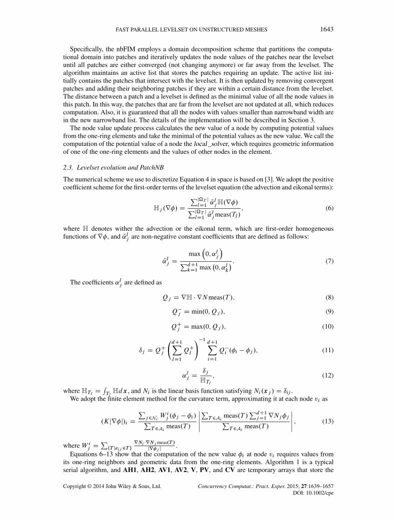
In both of the reinitialization and the evolution steps, we need to update the values of the nodesin the mesh, and these updates can be performed independently. The natural way to parallelize thecomputation is to assign each nodal update to a thread. We call this approach nodal parallelism, andit can be represented as a sparse matrix-vector operation as shown in Figure 1 (left). The operator

Ndenotes a generic operation defined on the degrees of freedom corresponding to ?’s. The advantageof this scheme is that it naturally avoids race conditions, because each nodal computation has anassociated thread. However, it can introduce unbalanced load when the nodes have widely varyingvalence. These irregular computations and data structures are not efficient on GPUs, because of thenature of the SIMD streaming architecture. An alternative parallelism scheme is to distribute compu-tations among threads according to the elements. We call such approach elemental parallelism; it ismore suitable for GPUs, because it gives regular local operators and corresponding data structures.Figure 1 (right) depicts the matrix representation of this approach: the matrix has a block structurein terms of local operators corresponding to the elements. The matrix blocks can overlap each other,and the vector of degrees of freedom is segmented but has overlaps. Each block matrix-vector oper-ation represents a set of local computations that are performed by a thread. This parallelism schememay result in race conditions as multiple threads may be updating the same degree of freedombecause of the overlapping. The conventional solution to this problems is to use atomic operations.



Figure 1. Matrix representations of the parallelism schemes. On the left, we present the nodal paral-lelism scheme. The ?’s denote non-zeros values or some operators. On the right, we present the elemental

parallelism scheme. The matrix is blocked, and the blocks can be overlapping each other.

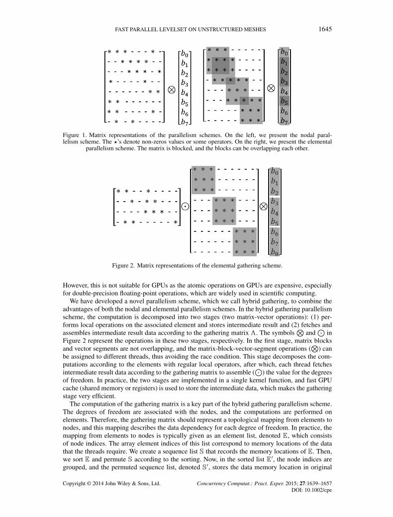
Figure 2. Matrix representations of the elemental gathering scheme.

However, this is not suitable for GPUs as the atomic operations on GPUs are expensive, especiallyfor double-precision floating-point operations, which are widely used in scientific computing.

We have developed a novel parallelism scheme, which we call hybrid gathering, to combine theadvantages of both the nodal and elemental parallelism schemes. In the hybrid gathering parallelismscheme, the computation is decomposed into two stages (two matrix-vector operations): (1) per-forms local operations on the associated element and stores intermediate result and (2) fetches andassembles intermediate result data according to the gathering matrix ƒ. The symbols

Nand

Jin

Figure 2 represent the operations in these two stages, respectively. In the first stage, matrix blocksand vector segments are not overlapping, and the matrix-block-vector-segment operations (

N) can

be assigned to different threads, thus avoiding the race condition. This stage decomposes the com-putations according to the elements with regular local operators, after which, each thread fetchesintermediate result data according to the gathering matrix to assemble (

J) the value for the degrees

of freedom. In practice, the two stages are implemented in a single kernel function, and fast GPUcache (shared memory or registers) is used to store the intermediate data, which makes the gatheringstage very efficient.

The computation of the gathering matrix is a key part of the hybrid gathering parallelism scheme.The degrees of freedom are associated with the nodes, and the computations are performed onelements. Therefore, the gathering matrix should represent a topological mapping from elements tonodes, and this mapping describes the data dependency for each degree of freedom. In practice, themapping from elements to nodes is typically given as an element list, denoted E, which consistsof node indices. The array element indices of this list correspond to memory locations of the datathat the threads require. We create a sequence list S that records the memory locations of E. Then,we sort E and permute S according to the sorting. Now, in the sorted list E0, the node indices aregrouped, and the permuted sequence list, denoted S0, stores the data memory location in original


1646 Z. FU ET AL.

element list E. The E0 and S0 together indicate the locations of the ?’s in the gathering matrix andform the coordinate list (COO) sparse matrix representation [21] of the gathering matrix. In this way,we convert the race condition problem to a sorting problem. Here, list E has fixed length keys, whichallows it to be sorted very efficiently on GPUs with radix sorting [19]. Essentially, sorting allows usto take full advantage of the GPU computing power and avoid the weakness of the architecture inthe form of addressing race conditions.

3. IMPLEMENTATION

In this section, we describe the implementation details of our method to solve the levelset equationson both shared memory CPU-based and GPU-based parallel systems. The pipeline consists of twostages: the setup stage and the time-stepping stage. The setup stage includes the partitioning of themesh into patches, preparation of the geometric data for the following computation and generationof ƒ. We choose the METIS software package [22] to perform the partitioning. METIS partitionsthe mesh into non-overlapping node patches and outputs a list showing the partition index of eachnode. The data-preparation step permutes the vertex coordinate list and rearranges the element listaccording to the partitioning. The time-stepping stage iteratively updates the node values until thedesired number of time-steps is reached. In each iteration, a reinitialization and multiple evolutionsteps are performed. We provide implementation details and data structures for the setup stage, thereinitialization step, and the evolution step, respectively, in the following subsections.

3.1. Setup

During the setup stage, the mesh is partitioned into patches, each of which consists of a set ofnodes and a set of elements according to METIS output. The sets of nodes are mutually exclusive,and the element sets are one-layer overlapping: the boundary elements are duplicated. The vertexcoordinate list and the element list are then permuted according to the partitioning so that the vertexcoordinates and the element vertex indices are grouped together, and hence, the global memoryaccess is coalesced.

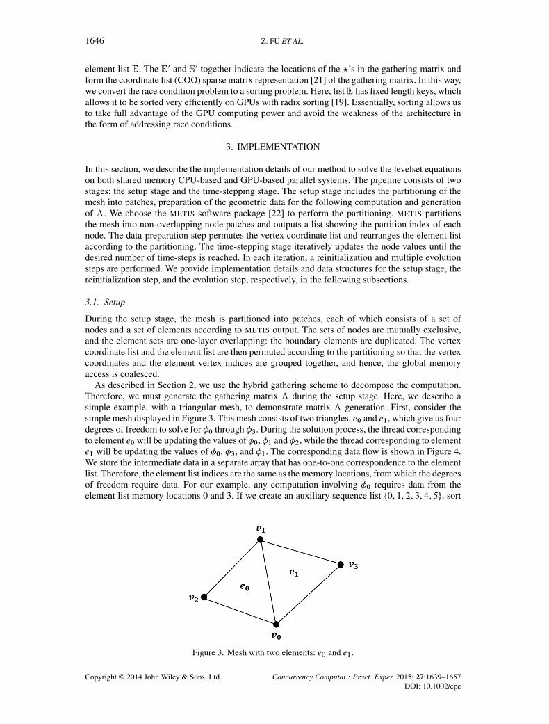
As described in Section 2, we use the hybrid gathering scheme to decompose the computation.Therefore, we must generate the gathering matrix ƒ during the setup stage. Here, we describe asimple example, with a triangular mesh, to demonstrate matrix ƒ generation. First, consider thesimple mesh displayed in Figure 3. This mesh consists of two triangles, e0 and e1, which give us fourdegrees of freedom to solve for �0 through �3. During the solution process, the thread correspondingto element e0 will be updating the values of �0, �1 and �2, while the thread corresponding to elemente1 will be updating the values of �0, �3, and �1. The corresponding data flow is shown in Figure 4.We store the intermediate data in a separate array that has one-to-one correspondence to the elementlist. Therefore, the element list indices are the same as the memory locations, from which the degreesof freedom require data. For our example, any computation involving �0 requires data from theelement list memory locations 0 and 3. If we create an auxiliary sequence list ¹0; 1; 2; 3; 4; 5º, sort

Figure 3. Mesh with two elements: e0 and e1.



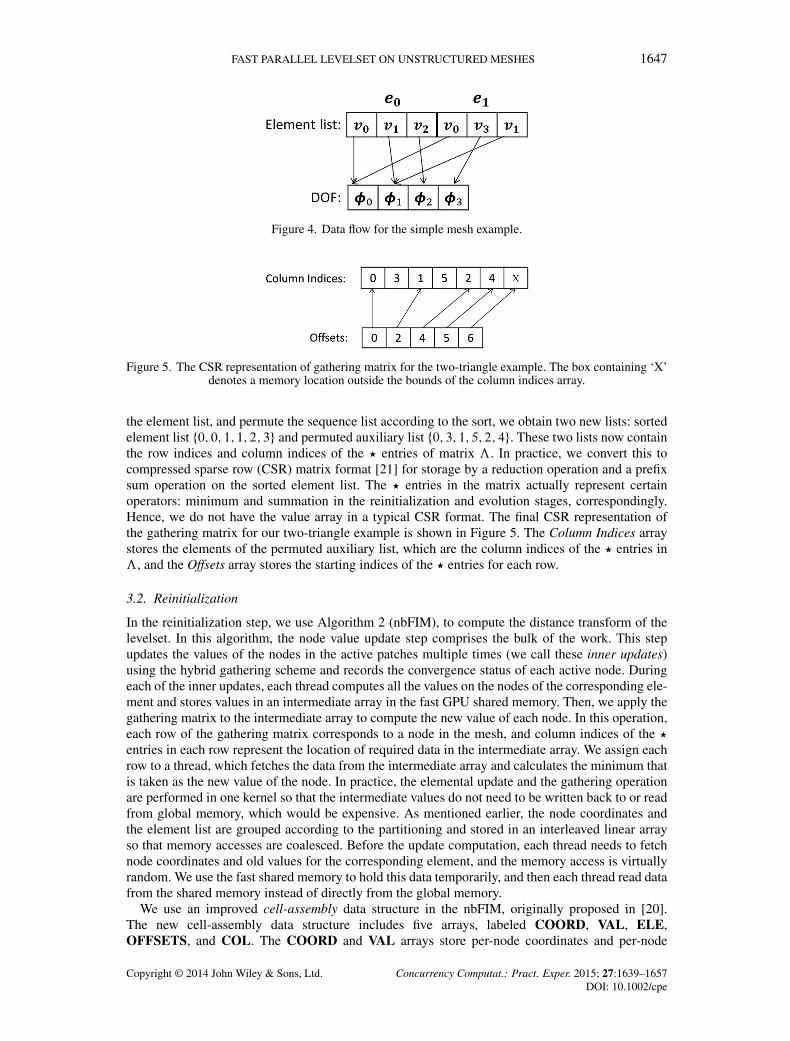
Figure 4. Data flow for the simple mesh example.

Figure 5. The CSR representation of gathering matrix for the two-triangle example. The box containing ‘X’denotes a memory location outside the bounds of the column indices array.

the element list, and permute the sequence list according to the sort, we obtain two new lists: sortedelement list ¹0; 0; 1; 1; 2; 3º and permuted auxiliary list ¹0; 3; 1; 5; 2; 4º. These two lists now containthe row indices and column indices of the ? entries of matrix ƒ. In practice, we convert this tocompressed sparse row (CSR) matrix format [21] for storage by a reduction operation and a prefixsum operation on the sorted element list. The ? entries in the matrix actually represent certainoperators: minimum and summation in the reinitialization and evolution stages, correspondingly.Hence, we do not have the value array in a typical CSR format. The final CSR representation ofthe gathering matrix for our two-triangle example is shown in Figure 5. The Column Indices arraystores the elements of the permuted auxiliary list, which are the column indices of the ? entries inƒ, and the Offsets array stores the starting indices of the ? entries for each row.

3.2. Reinitialization

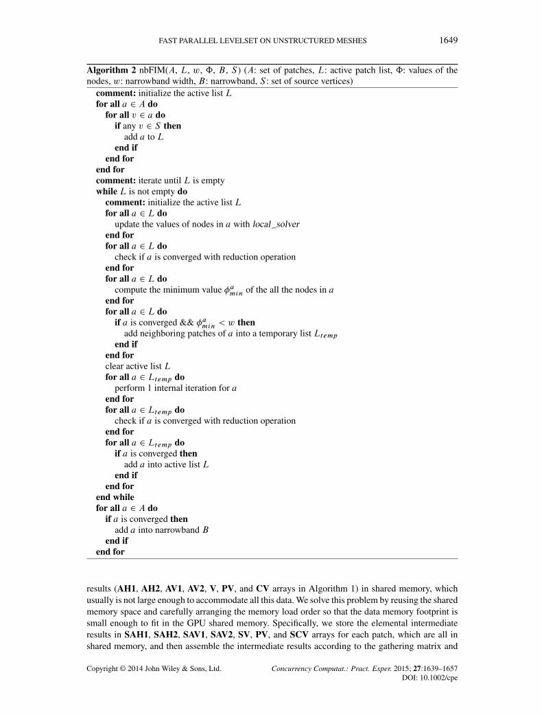
In the reinitialization step, we use Algorithm 2 (nbFIM), to compute the distance transform of thelevelset. In this algorithm, the node value update step comprises the bulk of the work. This stepupdates the values of the nodes in the active patches multiple times (we call these inner updates)using the hybrid gathering scheme and records the convergence status of each active node. Duringeach of the inner updates, each thread computes all the values on the nodes of the corresponding ele-ment and stores values in an intermediate array in the fast GPU shared memory. Then, we apply thegathering matrix to the intermediate array to compute the new value of each node. In this operation,each row of the gathering matrix corresponds to a node in the mesh, and column indices of the ?entries in each row represent the location of required data in the intermediate array. We assign eachrow to a thread, which fetches the data from the intermediate array and calculates the minimum thatis taken as the new value of the node. In practice, the elemental update and the gathering operationare performed in one kernel so that the intermediate values do not need to be written back to or readfrom global memory, which would be expensive. As mentioned earlier, the node coordinates andthe element list are grouped according to the partitioning and stored in an interleaved linear arrayso that memory accesses are coalesced. Before the update computation, each thread needs to fetchnode coordinates and old values for the corresponding element, and the memory access is virtuallyrandom. We use the fast shared memory to hold this data temporarily, and then each thread read datafrom the shared memory instead of directly from the global memory.

We use an improved cell-assembly data structure in the nbFIM, originally proposed in [20].The new cell-assembly data structure includes five arrays, labeled COORD, VAL, ELE,OFFSETS, and COL. The COORD and VAL arrays store per-node coordinates and per-node


1648 Z. FU ET AL.

value, respectively. ELE stores the per-element node indices. OFFSETS and COL form the CSRsparse matrix representation of the gathering matrix, except that we do not require a value array asin general CSR representation.

In summary, assuming that every patch has N nodes and M elements (normally M > N ), thereinitialization kernel function on the GPU (or SIMD parallelism) proceeds as follows:

(1) If thread index i < N , load the coordinates and value of node i into shared memory arraySHARE.

(2) If thread index i < M , load the node indices for element i from ELE into registers. Fetch thenode coordinates and values from SHARE to registers.

(3) If thread index i < M , write node values of element i to shared memory SHARE.(4) If thread index i < M , call local_solver routine to compute the potential values of each node

in element i and store these values in SHARE.(5) If thread index i < N , load the column indices for the i th row of the gathering matrix,

COL[OFFSETS[i]] through COL[OFFSETS[i C 1]]. Then fetch data from SHARE, com-pute the minimal value, and broadcast the minimal value to SHARE according to the columnindices.

(6) If thread index i < N , if the minimal value is the same as the old value (within a tolerance),node i is labeled convergent.

(7) Repeat steps 4 through 6 multiple times.(8) If thread index i < N , write the minimal value back to global memory VAL.

For CPU-based shared memory parallel system, the implementation is generally similar, but wemake several modifications from the GPU implementation to suit the CPU architecture. First, wemaintain an active node-group list instead of an active patch list. Each node-group in the list storesonly the active nodes in its corresponding patch instead of all nodes in the patch. The patched updatestrategy is suitable for GPU because it provides the fine-grained parallelism desired by the GPUarchitecture, but it also leads to extra computation [20]. Second, in the computation that updatesthe active node values, we assign each segment to a thread that updates all the active node val-ues in the segment. In addition, we use the nodal parallelism to avoid any race conditions. Eachthread computes the potential values of an active node from the one-ring elements and then calcu-lates the minimal value among the potential values. Specifically, the value update function in thereinitialization stage proceeds in the following steps for each thread t (here, P denotes the numberof patches):

(1) Load the coordinates and value �a of an active node a of the t th patch into registers.(2) Pick one of the one-ring elements of a and load the coordinates and values into registers.(3) Call the local_solver to compute a potential new value �tmp of node a and perform �a D

min.�a; �tmp/.(4) Repeat steps 2 and 3 until all one-ring elements of a are processed and write the final �a back

to memory.(5) Repeat steps 1–4 until all active nodes in patch t are processed.

3.3. Evolution

The evolution step updates the values of the nodes in the narrowband according to the equationspresented in Section 2. As shown in Algorithm 1, we compute the approximation of the three termsof F and then update the node values. Similar to the reinitialization step, we need to deal with mixedtypes of parallelism: nodal parallelism and elemental parallelism as elemental computations aresuitable for GPUs, but the degrees of freedom we want to solve for are defined on the nodes. Thehybrid gathering scheme is also used to solve this problem. The update of a node value depends onmultiple elemental computations corresponding to speed function F, and the computations for thethree terms of F all require the same geometric information and node values. Therefore, we want toperform all the computations in one kernel function to avoid repeated global memory access.

The hybrid gathering scheme is based on the assumption that the gathering is performed on fastshared memory, and using a single kernel means that we need to store all the elemental intermediate



Algorithm 2 nbFIM(A, L, w, ˆ, B , S ) (A: set of patches, L: active patch list, ˆ: values of thenodes, w: narrowband width, B: narrowband, S : set of source vertices)

comment: initialize the active list Lfor all a 2 A do

for all v 2 a doif any v 2 S then

add a to Lend if

end forend forcomment: iterate until L is emptywhile L is not empty do

comment: initialize the active list Lfor all a 2 L do

update the values of nodes in a with local_solverend forfor all a 2 L do

check if a is converged with reduction operationend forfor all a 2 L do

compute the minimum value �amin of the all the nodes in aend forfor all a 2 L do

if a is converged && �amin < w thenadd neighboring patches of a into a temporary list Ltemp

end ifend forclear active list Lfor all a 2 Ltemp do

perform 1 internal iteration for aend forfor all a 2 Ltemp do

check if a is converged with reduction operationend forfor all a 2 Ltemp do

if a is converged thenadd a into active list L

end ifend for

end whilefor all a 2 A do

if a is converged thenadd a into narrowband B

end ifend for

results (AH1, AH2, AV1, AV2, V, PV, and CV arrays in Algorithm 1) in shared memory, whichusually is not large enough to accommodate all this data. We solve this problem by reusing the sharedmemory space and carefully arranging the memory load order so that the data memory footprint issmall enough to fit in the GPU shared memory. Specifically, we store the elemental intermediateresults in SAH1, SAH2, SAV1, SAV2, SV, PV, and SCV arrays for each patch, which are all inshared memory, and then assemble the intermediate results according to the gathering matrix and


1650 Z. FU ET AL.

store them in fast registers. The evolution kernel function proceeds as follows (assuming every patchhas N nodes and M elements):

(1) If thread index t < N , load the coordinates and value of node t into shared memory arraySHARE.

(2) If thread index t < N , load the column indices for the t th row of the gathering matrix,COL[OFFSETS[t ]] through COL[OFFSETS[t C 1]] into registers.

(3) If thread index t < M , load the node indices for element t from ELE into registers. Fetchthe node coordinates and values from SHARE to registers.

(4) If thread index t < M , perform elemental computation of triangle Tijk for .H1/T , .H2/Tand Q̨1i , Q̨1j , Q̨1

k, Q̨2i , Q̨2j , Q̨2

k.

(5) If thread index t < M , compute SAH1[t*MC0] D Q̨1i � .H1/T , SAH1[t*MC1] D Q̨1j �

.H1/T , SAH1[t*MC2] D Q̨1k� .H1/T .

(6) If thread index t < N , fetch data from SAH1 according to the column indices for the t throw of the gathering matrix, compute the summation, and store the result in registers.

(7) If thread index t < M , compute SAH2[t*MC0] D Q̨2i � .H2/T , SAH2[t*MC1] D

Q̨2j � .H2/T , SAH2[t*MC2] D Q̨2

k� .H2/T . Note here SAH2 overlap SAH1 in the shared

memory space and the values of SAH2 are completely rewritten. In this way, the sharedmemory footprint is not increased as the size of SAH2 is the same as SAH1.

(8) If thread index t < N , fetch data from SAH1 according to the column indices for the t throw of the gathering matrix, compute the summation, and store the result in registers.

(9) Repeat steps 7 through 8 for SAV1, SAV2, SV, SPV, and SCV arrays.(10) If thread index t < N , compute the new value of node t .

Similarly, for the CPU implementation of the evolution step, we make certain modifications of theGPU implementation to suit the CPU architecture. We keep a list of elements that are inside thenarrowband and perform the computation only on these elements. This is different from the GPUimplementation, which updates all elements in a patch as long as any element in the patch is insidethe narrowband. We assign the element computations in each patch to a thread instead of eachelement to a thread to provide a coarse-grained parallelism for CPU. Also, we find that for CPU,atomic operations are sufficiently efficient, so the hybrid gathering scheme is not used.

3.4. Adaptive time-step computation

After each reinitialization step, we perform n update steps for the levelset evolution. In this process,we need to make sure that the evolving levelset does not cross the boundary of the narrowband.According to the Courant-Friedrichs-Lewy condition, the levelset evolution distance of each time-step �x � 2maxi<M .ri /, where ri denotes the inscribed circle or sphere of the i th element andM is the number of elements in the narrowband. Denoting the narrowband width as w, we make aconservative estimate of the number of steps n D w

4maxi<M .ri /, so that the levelset evolves at most

half of w. Because the narrowband is changing, max.ri / is also changing. Hence, we compute themax.ri / at the beginning of each reinitialization step: ri are pre-computed and stored in an array,and the max.ri / is computed with a reduction operation. In the evolution step, the time-step �t isdictated by the three terms of F in Equation 4. We define the time-step as

�t D mini<M

�2ri

d.j˛j C j�j

�;2r2id j�j

�; (14)

where d is the dimensionality of the mesh.

4. RESULTS AND DISCUSSION

In this section, we present numerical experiments to demonstrate the performance of the proposedalgorithms. We use a collection of 2D and 3D unstructured meshes of variable size and complex-ity to illustrate the performance of both CPU and GPU implementations. The performance data and



implementation related details are provided in the following order: (1) CPU implementation dis-cussion, (2) GPU implementation discussion, and concluded by (3) the comparison of the two. Forconsistency of evaluation, double precision is used in all algorithms and for all the experimentspresented in the following text.

The meshes used for the numerical experiments are

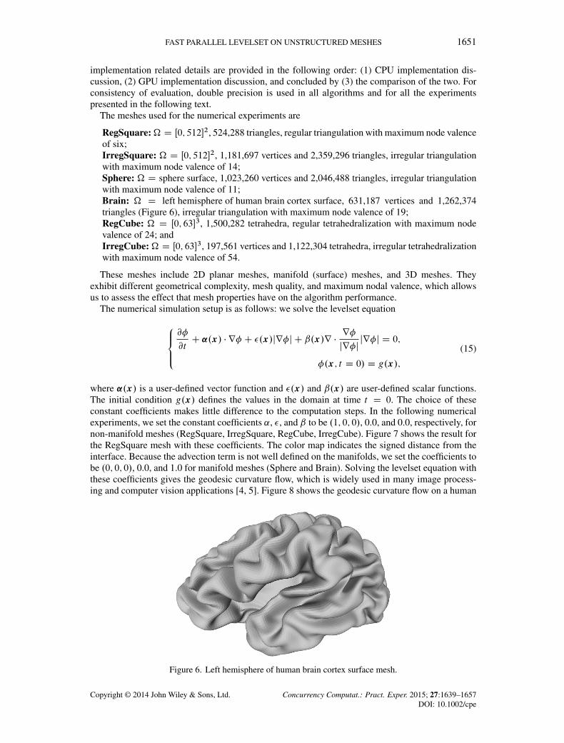
RegSquare:� D Œ0; 512�2, 524,288 triangles, regular triangulation with maximum node valenceof six;IrregSquare: � D Œ0; 512�2, 1,181,697 vertices and 2,359,296 triangles, irregular triangulationwith maximum node valence of 14;Sphere: � D sphere surface, 1,023,260 vertices and 2,046,488 triangles, irregular triangulationwith maximum node valence of 11;Brain: � D left hemisphere of human brain cortex surface, 631,187 vertices and 1,262,374triangles (Figure 6), irregular triangulation with maximum node valence of 19;RegCube: � D Œ0; 63�3, 1,500,282 tetrahedra, regular tetrahedralization with maximum nodevalence of 24; andIrregCube:� D Œ0; 63�3, 197,561 vertices and 1,122,304 tetrahedra, irregular tetrahedralizationwith maximum node valence of 54.

These meshes include 2D planar meshes, manifold (surface) meshes, and 3D meshes. Theyexhibit different geometrical complexity, mesh quality, and maximum nodal valence, which allowsus to assess the effect that mesh properties have on the algorithm performance.

The numerical simulation setup is as follows: we solve the levelset equation

8̂<:̂@�

@tC ˛.x/ � r� C �.x/jr�j C ˇ.x/r �

r�

jr�jjr�j D 0;

�.x; t D 0/ D g.x/;

(15)

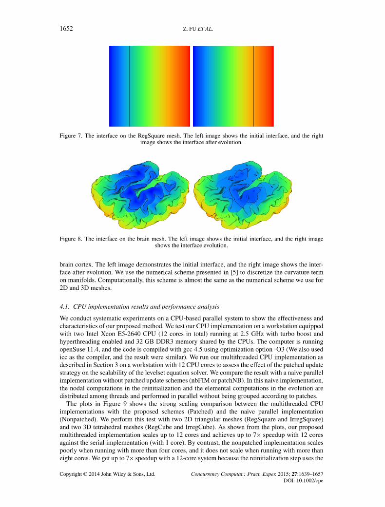
where ˛.x/ is a user-defined vector function and �.x/ and ˇ.x/ are user-defined scalar functions.The initial condition g.x/ defines the values in the domain at time t D 0. The choice of theseconstant coefficients makes little difference to the computation steps. In the following numericalexperiments, we set the constant coefficients ˛, �, and ˇ to be .1; 0; 0/, 0.0, and 0.0, respectively, fornon-manifold meshes (RegSquare, IrregSquare, RegCube, IrregCube). Figure 7 shows the result forthe RegSquare mesh with these coefficients. The color map indicates the signed distance from theinterface. Because the advection term is not well defined on the manifolds, we set the coefficients tobe .0; 0; 0/, 0.0, and 1.0 for manifold meshes (Sphere and Brain). Solving the levelset equation withthese coefficients gives the geodesic curvature flow, which is widely used in many image process-ing and computer vision applications [4, 5]. Figure 8 shows the geodesic curvature flow on a human

Figure 6. Left hemisphere of human brain cortex surface mesh.


1652 Z. FU ET AL.

Figure 7. The interface on the RegSquare mesh. The left image shows the initial interface, and the rightimage shows the interface after evolution.

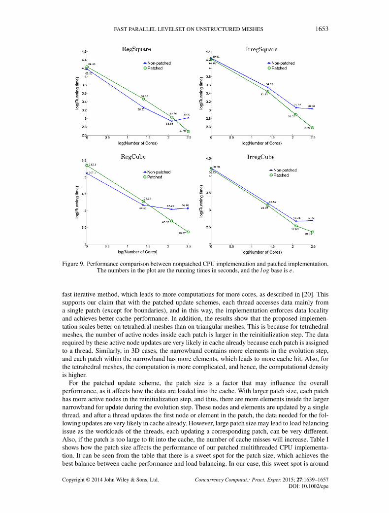
Figure 8. The interface on the brain mesh. The left image shows the initial interface, and the right imageshows the interface evolution.

brain cortex. The left image demonstrates the initial interface, and the right image shows the inter-face after evolution. We use the numerical scheme presented in [5] to discretize the curvature termon manifolds. Computationally, this scheme is almost the same as the numerical scheme we use for2D and 3D meshes.

4.1. CPU implementation results and performance analysis

We conduct systematic experiments on a CPU-based parallel system to show the effectiveness andcharacteristics of our proposed method. We test our CPU implementation on a workstation equippedwith two Intel Xeon E5-2640 CPU (12 cores in total) running at 2.5 GHz with turbo boost andhyperthreading enabled and 32 GB DDR3 memory shared by the CPUs. The computer is runningopenSuse 11.4, and the code is compiled with gcc 4.5 using optimization option -O3 (We also usedicc as the compiler, and the result were similar). We run our multithreaded CPU implementation asdescribed in Section 3 on a workstation with 12 CPU cores to assess the effect of the patched updatestrategy on the scalability of the levelset equation solver. We compare the result with a naive parallelimplementation without patched update schemes (nbFIM or patchNB). In this naive implementation,the nodal computations in the reinitialization and the elemental computations in the evolution aredistributed among threads and performed in parallel without being grouped according to patches.

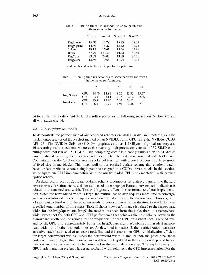
The plots in Figure 9 shows the strong scaling comparison between the multithreaded CPUimplementations with the proposed schemes (Patched) and the naive parallel implementation(Nonpatched). We perform this test with two 2D triangular meshes (RegSquare and IrregSquare)and two 3D tetrahedral meshes (RegCube and IrregCube). As shown from the plots, our proposedmultithreaded implementation scales up to 12 cores and achieves up to 7� speedup with 12 coresagainst the serial implementation (with 1 core). By contrast, the nonpatched implementation scalespoorly when running with more than four cores, and it does not scale when running with more thaneight cores. We get up to 7� speedup with a 12-core system because the reinitialization step uses the



Figure 9. Performance comparison between nonpatched CPU implementation and patched implementation.The numbers in the plot are the running times in seconds, and the log base is e.

fast iterative method, which leads to more computations for more cores, as described in [20]. Thissupports our claim that with the patched update schemes, each thread accesses data mainly froma single patch (except for boundaries), and in this way, the implementation enforces data localityand achieves better cache performance. In addition, the results show that the proposed implemen-tation scales better on tetrahedral meshes than on triangular meshes. This is because for tetrahedralmeshes, the number of active nodes inside each patch is larger in the reinitialization step. The datarequired by these active node updates are very likely in cache already because each patch is assignedto a thread. Similarly, in 3D cases, the narrowband contains more elements in the evolution step,and each patch within the narrowband has more elements, which leads to more cache hit. Also, forthe tetrahedral meshes, the computation is more complicated, and hence, the computational densityis higher.

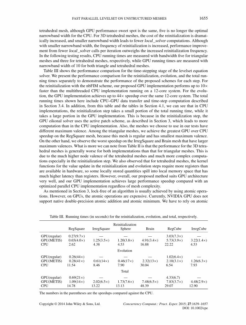
For the patched update scheme, the patch size is a factor that may influence the overallperformance, as it affects how the data are loaded into the cache. With larger patch size, each patchhas more active nodes in the reinitialization step, and thus, there are more elements inside the largernarrowband for update during the evolution step. These nodes and elements are updated by a singlethread, and after a thread updates the first node or element in the patch, the data needed for the fol-lowing updates are very likely in cache already. However, large patch size may lead to load balancingissue as the workloads of the threads, each updating a corresponding patch, can be very different.Also, if the patch is too large to fit into the cache, the number of cache misses will increase. Table Ishows how the patch size affects the performance of our patched multithreaded CPU implementa-tion. It can be seen from the table that there is a sweet spot for the patch size, which achieves thebest balance between cache performance and load balancing. In our case, this sweet spot is around


1654 Z. FU ET AL.

Table I. Running times (in seconds) to show patch sizeinfluence on performance.

Size 32 Size 64 Size 128 Size 256

RegSquare 15.40 14.78 15.35 18.78IrregSquare 14.89 13.22 15.42 19.22Sphere 18.15 15.02 15.66 17.86Brain 157.75 142.39 140.03 141.89RegCube 33.08 29.07 29.05 30.11IrregCube 12.89 10.63 11.24 11.78

Bold numbers denote the sweet spot for the patch size.

Table II. Running time (in seconds) to show narrowband widthinfluence on performance.

2 3 5 10 20

IrregSquare CPU 14.90 14.88 13.22 13.33 15.57GPU 3.13 3.14 2.75 2.12 2.46

IrregCube CPU 13.81 12.90 15.33 55.22 —GPU 6.13 5.75 4.94 4.48 7.01

64 for all the test meshes, and the CPU results reported in the following subsection (Section 4.2) areall with patch size 64.

4.2. GPU Performance results

To demonstrate the performance of our proposed schemes on SIMD parallel architectures, we haveimplemented and tested the levelset method on an NVIDIA Fermi GPU using the NVIDIA CUDAAPI [23]. The NVIDIA GeForce GTX 580 graphics card has 1.5 GBytes of global memory and16 streaming multiprocessors, where each streaming multiprocessors consists of 32 SIMD com-puting cores that run at 1.544 GHz. Each computing core has a configurable 16 or 48 KBytes ofon-chip shared memory, for quick access to local data. The code was compiled with NVCC 4.2.Computation on the GPU entails running a kernel function with a batch process of a large groupof fixed size thread blocks. This maps well to our patched update scheme that employs patch-based update methods, where a single patch is assigned to a CUDA thread block. In this section,we compare our GPU implementation with the multithreaded CPU implementation with patchedupdate scheme.

As described in Section 2, the narrowband scheme recomputes the distance transform to the zerolevelset every few time-steps, and the number of time-steps performed between reinitialization isrelated to the narrowband width. This width greatly affects the performance of our implementa-tion. When the narrowband width is large, the reinitialization step requires more time to converge,and each evolution step needs to update more nodes that are inside the narrowband. However, witha larger narrowband width, the program needs to perform fewer reinitialization to reach the user-specified total number of time-steps. Table II shows how performance is related to the narrowbandwidth for the IrregSquare and IrregCube meshes. As seen from the table, there is a narrowbandwidth sweet spot for both CPU and GPU performance that achieves the best balance between thenarrowband width and the reinitialization frequency. For the CPU, this sweet spot is around five,and for the GPU, it is approximately 10 for the IrregSquare mesh. We obtain similar ideal narrow-band width for all other triangular meshes. As described in Section 3, the reinitialization maintainsan active patch list instead of an active node list, and this makes our GPU reinitialization efficientfor larger narrowband widths. When the narrowband width is smaller than the patch size, thosenodes with values larger than narrowband width are not updated in the evolution step, and hence,their distance values need not to be computed in the reinitialization step. This explains why ourGPU implementation prefers a larger narrowband width relative to the CPU implementation. For the



tetrahedral mesh, although GPU performance sweet spot is the same, five is no longer the optimalnarrowband width for the CPU. For 3D tetrahedral meshes, the cost of the reinitialization is dramat-ically increased, and smaller narrowband width leads to fewer local_solver computations. Althoughwith smaller narrowband width, the frequency of reinitialization is increased, performance improve-ment from fewer local_solver calls per iteration outweighs the increased reinitialization frequency.In the following testing results, CPU running times are measured with bandwidth five for triangularmeshes and three for tetrahedral meshes, respectively, while GPU running times are measured withnarrowband width of 10 for both triangle and tetrahedral meshes.

Table III shows the performance comparison for the time-stepping stage of the levelset equationsolver. We present the performance comparison for the reinitialization, evolution, and the total run-ning times separately to demonstrate the performance of the proposed schemes for each step. Forthe reinitialization with the nbFIM scheme, our proposed GPU implementation performs up to 10�faster than the multithreaded CPU implementation running on a 12-core system. For the evolu-tion, the GPU implementation achieves up to 44� speedup over the same 12-core system. The totalrunning times shown here include CPU–GPU data transfer and time-step computation describedin Section 3.4. In addition, from this table and the tables in Section 4.1, we can see that in CPUimplementations, the reinitialization step takes a small portion of the total running time, while ittakes a large portion in the GPU implementation. This is because in the reinitialization step, theGPU eikonal solver uses the active patch scheme, as described in Section 3, which leads to morecomputation than in the CPU implementation. Also, the meshes we choose to use in our tests havedifferent maximum valence. Among the triangular meshes, we achieve the greatest GPU over CPUspeedup on the RegSquare mesh, because this mesh is regular and has smallest maximum valence.On the other hand, we observe the worst speedup on the IrregSquare and Brain mesh that have largermaximum valences. What is more we can note from Table II is that the performance for the 3D tetra-hedral meshes is generally worse for both implementations than that for triangular meshes. This isdue to the much higher node valence of the tetrahedral meshes and much more complex computa-tions especially in the reinitialization step. We also observed that for tetrahedral meshes, the kernelfunctions for the value update in the reinitialization and evolution steps require more registers thanare available in hardware, so some locally stored quantities spill into local memory space that hasmuch higher latency than registers. However, overall, our proposed method suits GPU architecturevery well, and our GPU implementation achieves large performance speedup compared with anoptimized parallel CPU implementation regardless of mesh complexity.

As mentioned in Section 3, lock-free of an algorithm is usually achieved by using atomic opera-tions. However, on GPUs, the atomic operations are expensive. Currently, NVIDIA GPU does notsupport native double-precision atomic addition and atomic minimum. We have to rely on atomic

Table III. Running times (in seconds) for the reinitialization, evolution, and total, respectively.

ReinitializationRegSquare IrregSquare Sphere Brain RegCube IrregCube

GPU(regular) 0.27(9.7�) — — — 3.03(7.3�) —GPU(METIS) 0.65(4.0�) 1.25(3.5�) 1.20(3.8�) 4.91(3.4�) 5.73(3.9�) 3.22(1.4�)CPU 2.62 4.38 4.53 16.88 22.22 4.53

Evolution

GPU(regular) 0.26(44�) — — — 1.02(6.4�) —GPU(METIS) 0.28(41�) 0.61(14�) 0.46(17�) 2.32(13�) 2.10(3.1�) 1.26(6.3�)CPU 11.54 8.46 7.90 30.04 6.54 7.93

Total

GPU(regular) 0.69(21�) — — — 4.33(6.7) —GPU(METIS) 1.09(14�) 2.02(6.5�) 1.73(7.6�) 7.48(6.5�) 7.83(3.7�) 4.48(2.9�)CPU 14.78 13.22 13.13 48.39 29.07 12.90

The numbers in the parentheses are the speedups compared against the CPU.


1656 Z. FU ET AL.

Table IV. Running times (in seconds) for the GPU implementations with hybrid gatheringand atomic operations.

RegSquare IrregSquare Sphere Brain RegCube IrregCube

Atomic 2.71 6.03 6.03 14.32 17.24 12.25Hybrid gathering 0.69 2.12 1.73 6.48 7.83 4.48Speedup 3.9� 2.8� 3.5� 2.2� 2.2� 2.7�

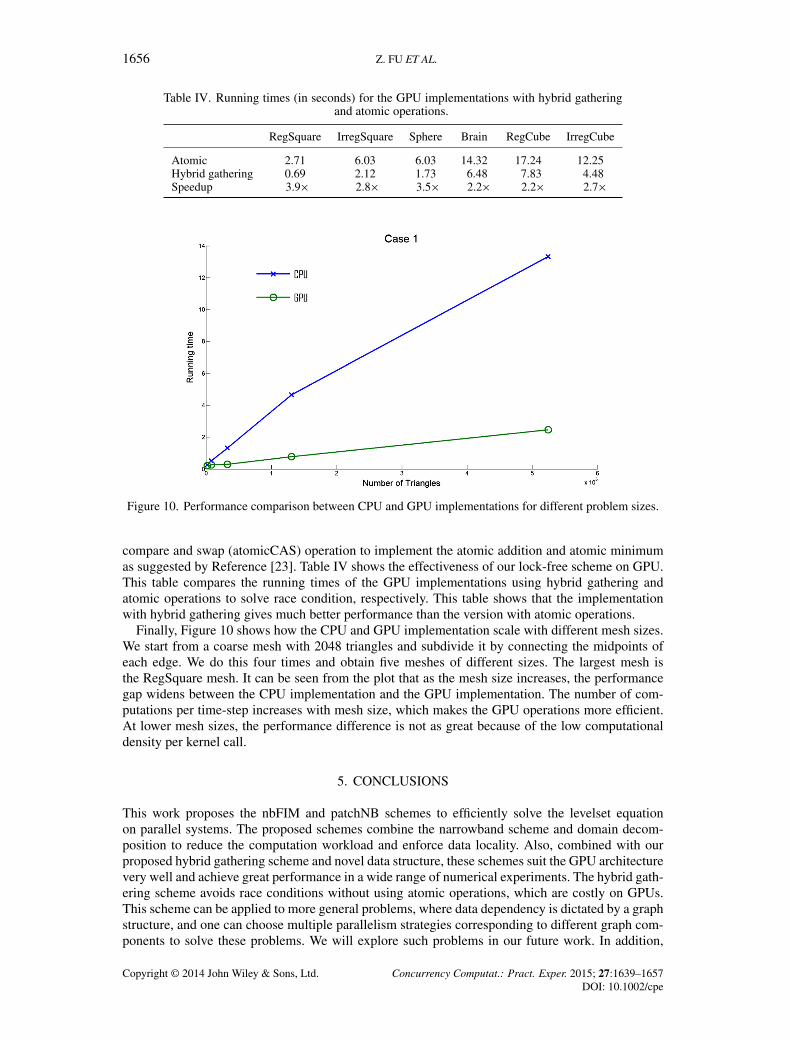
Figure 10. Performance comparison between CPU and GPU implementations for different problem sizes.

compare and swap (atomicCAS) operation to implement the atomic addition and atomic minimumas suggested by Reference [23]. Table IV shows the effectiveness of our lock-free scheme on GPU.This table compares the running times of the GPU implementations using hybrid gathering andatomic operations to solve race condition, respectively. This table shows that the implementationwith hybrid gathering gives much better performance than the version with atomic operations.

Finally, Figure 10 shows how the CPU and GPU implementation scale with different mesh sizes.We start from a coarse mesh with 2048 triangles and subdivide it by connecting the midpoints ofeach edge. We do this four times and obtain five meshes of different sizes. The largest mesh isthe RegSquare mesh. It can be seen from the plot that as the mesh size increases, the performancegap widens between the CPU implementation and the GPU implementation. The number of com-putations per time-step increases with mesh size, which makes the GPU operations more efficient.At lower mesh sizes, the performance difference is not as great because of the low computationaldensity per kernel call.

5. CONCLUSIONS

This work proposes the nbFIM and patchNB schemes to efficiently solve the levelset equationon parallel systems. The proposed schemes combine the narrowband scheme and domain decom-position to reduce the computation workload and enforce data locality. Also, combined with ourproposed hybrid gathering scheme and novel data structure, these schemes suit the GPU architecturevery well and achieve great performance in a wide range of numerical experiments. The hybrid gath-ering scheme avoids race conditions without using atomic operations, which are costly on GPUs.This scheme can be applied to more general problems, where data dependency is dictated by a graphstructure, and one can choose multiple parallelism strategies corresponding to different graph com-ponents to solve these problems. We will explore such problems in our future work. In addition,



for many real scientific and engineering applications, a single-node computer does not have enoughstorage or computing power to perform computations efficiently. We will thus work on extendingthe levelset equation solver to multiple GPUs and GPU clusters.

REFERENCES

1. Sethian JA. Level Set Methods and Fast Marching Methods. Cambridge University Press: Cambridge, 1999.2. Osher S, Sethian JA. Fronts propagating with curvature dependent speed: algorithms based on Hamilton–Jacobi

formulations. Journal of Computational Physics 1988; 79(1):12–49.3. Barth TJ, Sethian JA. Numerical schemes for the Hamilton–Jacobi and level set equations on triangulated domains,

1997.4. Joshi A, Shattuck D, Damasio H, Leahy R. Geodesic curvature flow on surfaces for automatic sulcal delineation. 9th

IEEE International Symposium on Biomedical Imaging (ISBI), 2012, Barcelona, 2012; 430–433.5. Wu C, Tai X. A level set formulation of geodesic curvature flow on simplicial surfaces. IEEE Transactions on

Visualization and Computer Graphics 2010; 16(4):647–662.6. Tan L, Zabaras N. A level set simulation of dendritic solidification of multi-component alloys. Journal of

Computational Physics 2007; 221(1):9–40. DOI: 10.1016/j.jcp.2006.06.003.7. Adalsteinsson D, Sethian JA. A fast level set method for propagating interfaces. Journal of Computational Physics

1995; 118(2):269–277. DOI: 10.1006/jcph.1995.1098.8. Whitaker RT. A level-set approach to 3D reconstruction from range data. International Journal of Computer Vision

1998; 29:203–231.9. Bridson RE. Computational aspects of dynamic surfaces. Ph.D. Thesis, Stanford University.

10. Strain J. Tree methods for moving interfaces. Journal of Computational Physics 1999; 151(2):616–648.11. Houston B, Nielsen MB, Batty C, Nilsson O, Museth K. Hierarchical RLE level set: a compact and versatile

deformable surface representation. ACM Transactions on Graphics 2006; 25(1):151–175.12. Lefohn A, Cates J, Whitaker R. Interactive, GPU-based level sets for 3D brain tumor segmentation. In Medical Image

Computing and Computer Assisted Intervention. MICCAI: Montréal, 2003; 564–572.13. Jeong WK, Beyer J, Hadwiger M, Vazquez A, Pfister H, Whitaker RT. Scalable and interactive segmentation and

visualization of neural processes in EM datasets. IEEE Transactions on Visualization and Computer Graphics 2009;15(6):1505–1514. DOI: 10.1109/TVCG.2009.178.

14. Fortmeier O, Bücker HM. A parallel strategy for a level set simulation of droplets moving in a liquid medium.Proceedings of the 9th International Conference on High Performance Computing for Computational Science,VECPAR’10, Springer-Verlag: Berlin, Heidelberg, 2011; 200–209. (Available from: http://dl.acm.org/citation.cfm?id=1964238.1964261) [Accessed on 22–25 June 2010].

15. Owen H, Houzeaux G, Samaniego C, Cucchietti F, Marin G, Tripiana C, Calmet H, Vazquez M. Two fluids level set:high performance simulation and post processing. 2012 SC Companion: High Performance Computing, Networking,Storage and Analysis (SCC), Salt Lake City, 2012; 1559–1568.

16. Rossi R, Larese A, Dadvand P, Oñate E. An efficient edge-based level set finite element method for free surface flowproblems. International Journal for Numerical Methods in Fluids 2013; 71(6):687–716. DOI: 10.1002/fld.3680.

17. Rodriguez JM, Sahni O, Lahey RT, Jr., Jansen KE. A parallel adaptive mesh method for the numerical simulation ofmultiphase flows. Computers & Fluids 2013; 87:115–131. DOI: http://dx.doi.org/10.1016/j.compfluid.2013.04.004.{USNCCM} Moving Boundaries.

18. Meuer H, Strohmaier E, Dongarra J, Simon H. Top500 supercomputer sites. (Available from: http://www.top500.org/) [Accessed on November 2013].

19. Satish N, Harris M, Garland M. Designing efficient sorting algorithms for manycore GPUs. NVIDIA Technical ReportNVR-2008-001, NVIDIA Corporation, September 2008.

20. Fu Z, Jeong WK, Pan Y, Kirby RM, Whitaker RT. A fast iterative method for solving the eikonal equation ontriangulated surfaces. SIAM Journal on Scientific Computing 2011; 33(5):2468–2488. DOI: 10.1137/100788951.

21. Bell N, Garland M. Efficient sparse matrix-vector multiplication on CUDA. NVIDIA Technical Report NVR-2008-004, NVIDIA Corporation, December 2008.

22. Karypis G, Kumar V. A fast and high quality multilevel scheme for partitioning irregular graphs. SIAM Journal onScientific Computing 1998; 20(1):359–392.

23. NVIDIA. Cuda programming guide. (Available from: http://www.nvidia.com/object/cuda.html) [Accessed onFebruary 2014].


http://dl.acm.org/citation.cfm?id=1964238.1964261

http://dl.acm.org/citation.cfm?id=1964238.1964261

http://www.top500.org/

http://www.top500.org/

http://www.nvidia.com/object/cuda.html

Documents

Fast parallel solver for the levelset equations on …kirby/Publications/Kirby-90.pdfFast parallel solver for the levelset equations on unstructured meshes Zhisong Fu*, †, Sergey