Journal of Computational Physics, vol 117, p 1–19 (1 March 1995)— originally Sandia Technical Report SAND91–1144 (May 1993, June 1994) —

Fast Parallel Algorithms

for

Short–Range Molecular Dynamics

Steve PlimptonParallel Computational Sciences Department 1421, MS 1111

Sandia National LaboratoriesAlbuquerque, NM 87185-1111

(505) 845-7873sjplimp@cs.sandia.gov

Keywords: molecular dynamics, parallel computing, N–body problem

Abstract

Three parallel algorithms for classical molecular dynamics are presented. The first assigns eachprocessor a fixed subset of atoms; the second assigns each a fixed subset of inter–atomic forces to compute;the third assigns each a fixed spatial region. The algorithms are suitable for molecular dynamics modelswhich can be difficult to parallelize efficiently — those with short–range forces where the neighbors ofeach atom change rapidly. They can be implemented on any distributed–memory parallel machine whichallows for message–passing of data between independently executing processors. The algorithms aretested on a standard Lennard–Jones benchmark problem for system sizes ranging from 500 to 100,000,000atoms on several parallel supercomputers — the nCUBE 2, Intel iPSC/860 and Paragon, and Cray T3D.Comparing the results to the fastest reported vectorized Cray Y–MP and C90 algorithm shows thatthe current generation of parallel machines is competitive with conventional vector supercomputers evenfor small problems. For large problems, the spatial algorithm achieves parallel efficiencies of 90% and a1840–node Intel Paragon performs up to 165 faster than a single Cray C90 processor. Trade–offs betweenthe three algorithms and guidelines for adapting them to more complex molecular dynamics simulationsare also discussed.

This work was partially supported by the Applied Mathematical Sciences program, U.S. Department of Energy, Office of

Energy Research, and was performed at Sandia National Laboratories, operated for the DOE under contract No. DE–AC04–

76DP00789.

The three parallel benchmark codes used in this study are available from the author via e–mail or on the world-wide web

at http://www.cs.sandia.gov/∼sjplimp/main.html

1

1 Introduction

Classical molecular dynamics (MD) is a commonly used computational tool for simulating the properties

of liquids, solids, and molecules [1, 2]. Each of the N atoms or molecules in the simulation is treated as

a point mass and Newton’s equations are integrated to compute their motion. From the motion of the

ensemble of atoms a variety of useful microscopic and macroscopic information can be extracted such as

transport coefficients, phase diagrams, and structural or conformational properties. The physics of the

model is contained in a potential energy functional for the system from which individual force equations for

each atom are derived.

MD simulations are typically not memory intensive since only vectors of atom information are stored.

Computationally, the simulations are “large” in two domains — the number of atoms and number of

timesteps. The length scale for atomic coordinates is Angstroms; in three dimensions many thousands

or millions of atoms must usually be simulated to approach even the sub–micron scale. In liquids and solids

the timestep size is constrained by the demand that the vibrational motion of the atoms be accurately

tracked. This limits timesteps to the femtosecond scale and so tens or hundreds of thousands of timesteps

are necessary to simulate even picoseconds of “real” time. Because of these computational demands, con-

siderable effort has been expended by researchers to optimize MD calculations for vector supercomputers

[24, 30, 36, 45, 47] and even to build special–purpose hardware for performing MD simulations [4, 5]. The

current state–of–the–art is such that simulating ten– to hundred–thousand atom systems for picoseconds

takes hours of CPU time on machines such as the Cray Y–MP.

The fact that MD computations are inherently parallel has been extensively discussed in the literature

[11, 22]. There has been considerable effort in the last few years by researchers to exploit this parallelism

on various machines. The majority of the work that has included implementations of proposed algorithms

has been for single–instruction/multiple–data (SIMD) parallel machines such as the CM–2 [12, 52], or for

multiple–instruction/multiple–data (MIMD) parallel machines with a few dozens of processors [26, 37, 39, 46].

Recently there have been efforts to create scalable algorithms that work well on hundred– to thousand–

processor MIMD machines [9, 14, 20, 41, 51]. We are convinced that the message–passing model of pro-

gramming for MIMD machines is the only one that provides enough flexibility to implement all the data

structure and computational enhancements that are commonly exploited in MD codes on serial and vector

machines. Also, we have found that it is only the current generation of massively parallel MIMD machines

with hundreds to thousands of processors that have the computational power to be competitive with the

fastest vector machines for MD calculations.

In this paper we present three parallel algorithms which are appropriate for a general class of MD problems

that has two salient characteristics. The first characteristic is that forces are limited in range, meaning each

atom interacts only with other atoms that are geometrically nearby. Solids and liquids are often modeled

this way due to electronic screening effects or simply to avoid the computational cost of including long–range

Coulombic forces. For short–range MD the computational effort per timestep scales as N , the number of

2

atoms.

The second characteristic is that the atoms can undergo large displacements over the duration of the

simulation. This could be due to diffusion in a solid or liquid or conformational changes in a biological

molecule. The important feature from a computational standpoint is that each atom’s neighbors change as

the simulation progresses. While the algorithms we discuss could also be used for fixed–neighbor simulations

(e.g. all atoms remain on lattice sites in a solid), it is a harder task to continually track the neighbors of

each atom and maintain efficient O(N) scaling for the overall computation on a parallel machine.

Our first goal in this effort was to develop parallel algorithms that would be competitive with the fastest

methods on vector supercomputers such as the Cray. Moreover we wanted the algorithms to work well

on problems with small numbers of atoms, not just for large problems where parallelism is often easier to

exploit. This is because the vast majority of MD simulations are performed on systems of a few hundred to

several thousand atoms where N is chosen to be as small as possible while still accurate enough to model

the desired physical effects [8, 44, 38, 53]. The computational goal in these calculations is to perform each

timestep as quickly as possible. This is particularly true in non–equilibrium MD where macroscopic changes

in the system may take significant time to evolve, requiring millions of timesteps to model. Thus, it is often

more useful to be able to perform a 100, 000 timestep simulation of a 1000 atom system fast rather than

1000 timesteps of a 100, 000 atom system, though the O(N) scaling means the computational effort is the

same for both cases. To this end, we consider model sizes as small as a few hundred atoms in this paper.

For very large MD problems, our second goal in this work was to develop parallel algorithms that would

be scalable to larger and faster parallel machines. While the timings we present for large MD models (105

to 108 atoms) on the current generation of parallel supercomputers (hundreds to thousands of processors)

are quite fast compared to vector supercomputers, they are still too slow to allow long–timescale simulations

to be done routinely. However, our large–system algorithm scales optimally with respect to N and P (the

number of processors) so that as parallel machines become more powerful in the next few years, algorithms

similar to it will enable larger problems to be studied.

Our earlier efforts in this area [40] produced algorithms which were fast for systems with up to tens of

thousands of atoms but did not scale optimally with N for larger systems. We improved on this effort to create

a scalable large–system algorithm in [41]. The spatial–decomposition algorithm we present here is also unique

in that it performs well on relatively small problems (only a few atoms per processor). In addition, we have

added an idea due to Tamayo and Giles [51] that has improved the algorithm’s performance on medium–sized

problems by reducing the inter–processor communication requirements. We have also recently developed a

new parallel algorithm (force–decomposition) which we present here in the context of MD simulations for

the first time. It offers the advantages of both simplicity and speed for small to medium–sized problems.

In the next section, the computational aspects of MD are highlighted and efforts to speed the calculations

on vector and parallel machines are briefly reviewed. In Sections 3, 4, and 5 we describe our three parallel

algorithms in detail. A standard Lennard–Jones benchmark calculation is outlined in Section 6. In Section

3

7, implementation details and timing results for the parallel algorithms on several massively parallel MIMD

machines are given and comparisons made to Cray Y–MP and C90 timings for the benchmark calculation.

Discussion of the scaling properties of the algorithms is also included. Finally, in Section 8, we give guidelines

for deciding which parallel algorithm is likely to be fastest for a particular short–range MD simulation.

2 Computational Aspects of Molecular Dynamics

The computational task in a MD simulation is to integrate the set of coupled differential equations (Newton’s

equations) given by

mid~vi

dt=

∑j

F2(~ri, ~rj) +∑

j

∑k

F3(~ri, ~rj , ~rk) + · · · (1)

d~ri

dt= ~vi

where mi is the mass of atom i, ~ri and ~vi are its position and velocity vectors, F2 is a force function describing

pairwise interactions between atoms, F3 describes three–body interactions, and many–body interactions can

be added. The force terms are derivatives of energy expressions in which the energy of atom i is typically

written as a function of the positions of itself and other atoms. In practice, only one or a few terms in

equation (1) are kept and F2, F3, etc. are constructed so as to include many–body and quantum effects. To

the extent the approximations are accurate these equations give a full description of the time–evolution of

the system. Thus, the great computational advantage of classical MD, as compared to ab initio electronic

structure calculations, is that the dynamic behavior of the atomic system is described empirically without

having to solve Schrodinger’s equation at each timestep.

The force terms in equation (1) are typically non–linear functions of the distance rij between pairs of

atoms and may be either long–range or short–range in nature. For long–range forces, such as Coulombic

interactions in an ionic solid or biological system, each atom interacts with all others. Directly computing

these forces scales as N2 and is too costly for large N . Various approximate methods overcome this difficulty.

They include particle–mesh algorithms [31] which scale as f(M)N where M is the number of mesh points,

hierarchical methods [6] which scale as N log(N), and fast–multipole methods [23] which scale as N . Recent

parallel implementations of these algorithms [19, 56] have improved their range of applicability for many–

body simulations, but because of their expense, long–range force models are not commonly used in classical

MD simulations.

By contrast, short–range force models are used extensively in MD and is what we are concerned with

in this paper. They are chosen either because electronic screening effectively limits the range of influence

of the interatomic forces being modeled or simply to truncate the long–range interactions and lessen the

computational load. In either case, the summations in equation (1) are restricted to atoms within some

small region surrounding atom i. This is typically implemented using a cutoff distance rc, outside of which

4

all interactions are ignored. The work to compute forces now scales linearly with N . Notwithstanding this

savings, the vast majority of computation time spent in a short–range force MD simulation is in evaluating the

force terms in equation (1). The time integration typically requires only 2-3% of the total time. To evaluate

the sums efficiently requires knowing which atoms are within the cutoff distance rc at every timestep. The

key is to minimize the number of neighboring atoms that must be checked for possible interactions since

calculations performed on neighbors at a distance r > rc are wasted computation. There are two basic

techniques used to accomplish this on serial and vector machines; we discuss them briefly here since our

parallel algorithms incorporate similar ideas.

The first idea, that of neighbor lists, was originally proposed by Verlet [55]. For each atom, a list is

maintained of nearby atoms. Typically, when the list is formed, all neighboring atoms within an extended

cutoff distance rs = rc + δ are stored. The list is used for a few timesteps to calculate all force interactions.

Then it is rebuilt before any atom could have moved from a distance r > rs to r < rc. Though δ is always

chosen to be small relative to rc, an optimal value depends on the parameters (e.g. temperature, diffusivity,

density) of the particular simulation. The advantage of the neighbor list is that once it is built, examining

it for possible interactions is much faster than checking all atoms in the system.

The second technique commonly used for speeding up MD calculations is known as the link-cell method

[32]. At every timestep, all the atoms are binned into 3–D cells of side length d where d = rc or slightly

larger. This reduces the task of finding neighbors of a given atom to checking in 27 bins — the bin the atom

is in and the 26 surrounding ones. Since binning the atoms only requires O(N) work, the extra overhead

associated with it is acceptable for the savings of only having to check a local region for neighbors.

The fastest MD algorithms on serial and vector machines use a combination of neighbor lists and link–cell

binning. In the combined method, atoms are only binned once every few timesteps for the purpose of forming

neighbor lists. In this case atoms are binned into cells of size d ≥ rs. At intermediate timesteps the neighbor

lists alone are used in the usual way to find neighbors within a distance rc of each atom. This is a significant

savings over a conventional link–cell method since there are far fewer atoms to check in a sphere of volume

4πrs3/3 than in a cube of volume 27rc

3. Additional savings can be gained due to Newton’s 3rd law by only

computing a force once for each pair of atoms (rather than once for each atom in the pair). In the combined

method this is done by only searching half the surrounding bins of each atom to form its neighbor list. This

has the effect of storing atom j in atom i’s list, but not atom i in atom j’s list, thus halving the number of

force computations that must be done.

Although these ideas are simply described, optimal performance on a vector machine requires careful

attention to data structures and loop constructs to insure complete vectorization. The fastest implementation

reported in the literature is that of Grest, et al. [24]. They use the combined neighbor list/link–cell method

described above to create long lists of pairs of neighboring atoms. At each timestep, they prune the lists to

keep only those pairs within the cutoff distance rc. Finally, they organize the lists into packets in which no

atom appears twice [45]. The force computation for each packet can then be completely vectorized, resulting

5

in performance on the benchmark problem described in Section 6 that is from 2 to 10 times faster than other

vectorized algorithms [20, 30, 47] over a wide range of simulation sizes.

In recent years there has been considerable interest in devising parallel MD algorithms. The natural

parallelism in MD is that the force calculations and velocity/position updates can be done simultaneously

for all atoms. To date, two basic ideas have been exploited to achieve this parallelism. The goal in each

is to divide the force computations in equation (1) evenly across the processors so as to extract maximum

parallelism. To our knowledge, all algorithms that have been proposed or implemented (including ours) have

been variations on these two methods. References [21, 25, 49] include good overviews of various techniques.

In the first class of methods a pre–determined set of force computations is assigned to each processor.

The assignment remains fixed for the duration of the simulation. The simplest way of doing this is to give a

subgroup of atoms to each processor. We call this method an atom–decomposition of the workload, since the

processor computes forces on its atoms no matter where they move in the simulation domain. More generally,

a subset of the force loops inherent in equation (1) can be assigned to each processor. We term this a force–

decomposition and describe a new algorithm of this type later in the paper. Both of these decompositions are

analogous to Lagrangian gridding in a fluids simulations where the grid cells (computational elements) move

with the fluid (atoms in MD). By contrast, in the second general class of methods, which we call a spatial–

decomposition of the workload, each processor is assigned a portion of the physical simulation domain. Each

processor computes only the forces on atoms in its sub–domain. As the simulation progresses processors

exchange atoms as they move from one sub–domain to another. This is analogous to an Eulerian gridding

for a fluids simulation where the grid remains fixed in space as fluid moves through it.

Within the two classes of methods for parallelization of MD, a variety of algorithms have been proposed

and implemented by various researchers. The details of the algorithms vary widely from one parallel machine

to another since there are numerous problem–dependent and machine–dependent trade–offs to consider, such

as the relative speeds of computation and communication. A brief review of some notable efforts follows.

Atom–decomposition methods, also called replicated–data methods [49] because identical copies of atom

information are stored on all processors, are often used in MD simulations of molecular systems. This is

because the duplication of information makes for straight–forward computation of additional three– and four–

body force terms. Parallel implementations of state–of–the–art biological MD programs such as CHARMM

and GROMOS using this technique are discussed in [13, 17]. Force–decomposition methods which systolically

cycle atom data around a ring or through a grid of processors have been used on MIMD [26, 49] and SIMD

machines [16, 57]. Other force–decomposition methods that use the force–matrix formalism we discuss in

Sections 3 and 4 have been presented in [12] and [15]. Boyer and Pawley [12] decompose the force matrix by

sub–blocks, while the method of Brunet, et al. [15] partitions the matrix element by element. In both cases

their methods are designed for long–range force systems requiring all–pairs calculations (no neighbor lists)

on SIMD machines. Thus the scaling of these algorithms is different from the algorithm presented in Section

4 as is the way they distribute the atom data among processors and perform inter–processor communication.

6

Spatial–decomposition methods, also called geometric methods [21, 25], are more common in the literature

because they are well–suited to very large MD simulations. Recent parallel message–passing implementations

for the Intel iPSC/2 hypercube [39, 46, 49], CM–5 [9, 51], Fujitsu AP1000 [14], and a T800 Transputer

machine [20] have some features in common with the spatial–decomposition algorithm we present in Section

5. Our algorithm has the additional capability of working well in the regime where a processor’s sub–domain

is smaller than the force cutoff distance.

The fastest published algorithms for SIMD machines also employ spatial–decomposition techniques [52].

However, the data–parallel programming model, which on SIMD machines requires processors executing each

statement to operate simultaneously on a global data structure, introduces inefficiencies in short–range MD

algorithms, particularly when coding the construction and access of variable–length neighbor lists via indirect

addressing. Thus the timings in [52] for the benchmark problem discussed in Section 6 on a 32K–processor

CM–2 are slower than the single–processor Cray Y–MP timings presented in Section 7. By contrast, the

timings for the message–passing parallel algorithms in this paper and references [9, 14, 51] are considerably

faster, indicating the advantage a message–passing paradigm offers for exploiting parallelism in short–range

MD simulations.

3 Atom–Decomposition Algorithm

In our first parallel algorithm each of the P processors is assigned a group of N/P atoms at the beginning

of the simulation. Atoms in a group need not have any special spatial relationship to each other. For ease

of exposition, we assume N is a multiple of P , though it is simple to relax this constraint. A processor will

compute forces on only its N/P atoms and will update their positions and velocities for the duration of the

simulation no matter where they move in the physical domain. As discussed in the previous section, this is

an atom–decomposition (AD) of the computational workload.

A useful construct for representing the computational work involved in the algorithm is the N ×N force

matrix F . The (ij) element of F represents the force on atom i due to atom j. Note that F is sparse due to

short–range forces and skew–symmetric, i.e. Fij = −Fji, due to Newton’s 3rd law. We also define x and f

as vectors of length N which store the position and total force on each atom. For a 3–D simulation, xi would

store the three coordinates of atom i. With these definitions, the AD algorithm assigns each processor a

sub–block of F which consists of N/P rows of the matrix, as shown in Figure 1. If z indexes the processors

from 0 to P −1, then processor Pz computes matrix elements in the Fz sub–block of rows. It also is assigned

the corresponding sub–vectors of length N/P denoted by xz and fz.

Assume the computation of matrix element Fij requires only the two atom positions xi and xj . (We relax

this assumption in Section 8.) To compute all the elements in Fz, processor Pz will need the positions of

many atoms owned by other processors. In Figure 1 this is represented by having the horizontal vector x at

the top of the figure span all the columns of F . This implies that every timestep each processor must receive

updated atom positions from all the other processors, an operation called all–to–all communication. Various

7

algorithms have been developed for performing this operation efficiently on different parallel machines and

architectures [7, 22, 54]. We use an idea outlined in Fox, et al. [22] that is simple, portable, and works well

on a variety of machines. We describe it briefly because it is the chief communication component of both

the AD algorithms of this section and the force–decomposition algorithms presented in the next section.

Following Fox’s nomenclature, we term the all–to–all communication procedure an expand operation.

Each processor allocates memory of length N to store the entire x vector. At the beginning of the expand,

processor Pz has xz, an updated piece of x of length N/P . Each processor needs to acquire all the other

processor’s pieces, storing them in the correct places in its copy of x. Figure 2a illustrates the steps that

accomplish this for an 8–processor example. The processors are mapped consecutively to the sub–pieces of

the vector. In the first communication step, each processor partners with an adjacent processor in the vector

and they exchange sub–pieces. Processor 2 partners with 3. Now, every processor has a contiguous piece

of x that is of length 2N/P . In the second step, each processor partners with a processor two positions

away and exchanges its new piece (2 receives the shaded sub–vectors from 0). Each processor now has a

4N/P–length piece of x. In the last step, each processor exchanges an N/2–length piece of x with a processor

P/2 positions away (2 exchanges with 6); the entire vector now resides on each processor.

A communication operation that is essentially the inverse of the expand will also prove useful in both the

atom– and force–decomposition algorithms. Assume each processor has stored new force values throughout

its copy of the force vector f . Processor Pz needs to know the N/P values in fz, where each of the values is

summed across all P processors. This is known as a fold operation [22] and is outlined in Figure 2b. In the

first step each processor exchanges half the vector with a processor it partners with that is P/2 positions

away. Note that each processor receives the half that it is a member of and sends the half it is not a member

of (processor 2 receives the shaded first half of the vector from 6). Each processor sums the received values

with its corresponding retained sub–vector. This operation is recursed, halving the length of the exchanged

data at each step.

Costs for a communication algorithm are typically quantified by the number of messages and the total

volume of data sent and received. On both these accounts the expand and fold of Figure 2 are optimal; each

processor performs log2(P ) sends and receives and exchanges N − N/P data values. Each processor also

performs N −N/P additions in the fold. A drawback is that the algorithms require O(N) storage on every

processor. Alternative methods for performing all–to–all communication require less storage at the cost of

more sends and receives. This is usually not a good trade–off for MD simulations because, as we shall see,

quite large problems can be run with the many Mbytes of local memory available on current–generation

processors.

We now present two versions of an AD algorithm which use expand and fold operations. The first is

simpler and does not take advantage of Newton’s 3rd law. We call this algorithm A1; it is outlined in Figure

3 with the dominating term(s) in the computation or communication cost of each step listed on the right.

We assume at the beginning of the timestep that each processor knows the current positions of all N atoms,

8

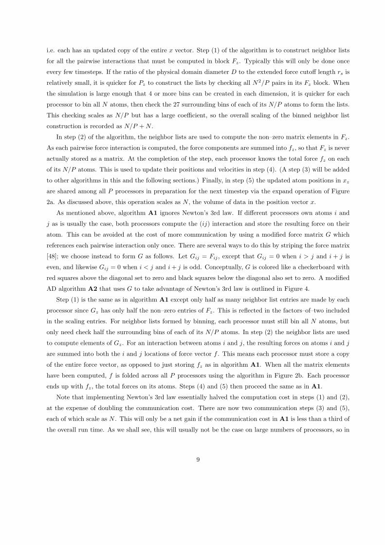
i.e. each has an updated copy of the entire x vector. Step (1) of the algorithm is to construct neighbor lists

for all the pairwise interactions that must be computed in block Fz. Typically this will only be done once

every few timesteps. If the ratio of the physical domain diameter D to the extended force cutoff length rs is

relatively small, it is quicker for Pz to construct the lists by checking all N2/P pairs in its Fz block. When

the simulation is large enough that 4 or more bins can be created in each dimension, it is quicker for each

processor to bin all N atoms, then check the 27 surrounding bins of each of its N/P atoms to form the lists.

This checking scales as N/P but has a large coefficient, so the overall scaling of the binned neighbor list

construction is recorded as N/P + N .

In step (2) of the algorithm, the neighbor lists are used to compute the non–zero matrix elements in Fz.

As each pairwise force interaction is computed, the force components are summed into fz, so that Fz is never

actually stored as a matrix. At the completion of the step, each processor knows the total force fz on each

of its N/P atoms. This is used to update their positions and velocities in step (4). (A step (3) will be added

to other algorithms in this and the following sections.) Finally, in step (5) the updated atom positions in xz

are shared among all P processors in preparation for the next timestep via the expand operation of Figure

2a. As discussed above, this operation scales as N , the volume of data in the position vector x.

As mentioned above, algorithm A1 ignores Newton’s 3rd law. If different processors own atoms i and

j as is usually the case, both processors compute the (ij) interaction and store the resulting force on their

atom. This can be avoided at the cost of more communication by using a modified force matrix G which

references each pairwise interaction only once. There are several ways to do this by striping the force matrix

[48]; we choose instead to form G as follows. Let Gij = Fij , except that Gij = 0 when i > j and i + j is

even, and likewise Gij = 0 when i < j and i + j is odd. Conceptually, G is colored like a checkerboard with

red squares above the diagonal set to zero and black squares below the diagonal also set to zero. A modified

AD algorithm A2 that uses G to take advantage of Newton’s 3rd law is outlined in Figure 4.

Step (1) is the same as in algorithm A1 except only half as many neighbor list entries are made by each

processor since Gz has only half the non–zero entries of Fz. This is reflected in the factors–of–two included

in the scaling entries. For neighbor lists formed by binning, each processor must still bin all N atoms, but

only need check half the surrounding bins of each of its N/P atoms. In step (2) the neighbor lists are used

to compute elements of Gz. For an interaction between atoms i and j, the resulting forces on atoms i and j

are summed into both the i and j locations of force vector f . This means each processor must store a copy

of the entire force vector, as opposed to just storing fz as in algorithm A1. When all the matrix elements

have been computed, f is folded across all P processors using the algorithm in Figure 2b. Each processor

ends up with fz, the total forces on its atoms. Steps (4) and (5) then proceed the same as in A1.

Note that implementing Newton’s 3rd law essentially halved the computation cost in steps (1) and (2),

at the expense of doubling the communication cost. There are now two communication steps (3) and (5),

each of which scale as N . This will only be a net gain if the communication cost in A1 is less than a third of

the overall run time. As we shall see, this will usually not be the case on large numbers of processors, so in

9

practice we almost always choose A1 instead of A2 for an AD algorithm. However, for small P or expensive

force models, A2 can be faster.

Finally, we discuss the issue of load–balance. Each processor will have an equal amount of work if each

Fz or Gz block has roughly the same number of non–zero elements. This will be the case if the atom density

is uniform across the simulation domain. However non–uniform densities can arise if, for example, there

are free surfaces so that some atoms border on vacuum, or phase changes are occurring within a liquid or

solid. This is only a problem for load–balance if the N atoms are ordered in a geometric sense as is typically

the case. Then a group of N/P atoms near a surface, for example, will have fewer neighbors than groups

in the interior. This can be overcome by randomly permuting the atom ordering at the beginning of the

simulation, which is equivalent to permuting rows and columns of F or G. This insures that every Fz or

Gz will have roughly the same number of non–zeros. A random permutation also has the advantage that

the load–balance will likely persist as atoms move about during the simulation. Note that this permutation

need only be done once, as a pre–processing step before beginning the dynamics.

In summary, the AD algorithms divide the MD force computation and integration evenly across the pro-

cessors (ignoring the O(N) component of binned neighbor list construction which is usually not significant).

However, the algorithms require global communication, as each processor must acquire information held by

all the other processors. This communication scales as N , independent of P , so it limits the number of

processors that can be used effectively. The chief advantage of the algorithms is that of simplicity. Steps

(1), (2), and (4) can be implemented by simply modifying the loops and data structures in a serial or vector

code to treat N/P atoms instead of N . The expand and fold communication operations (3) and (5) can

be treated as black–box routines and inserted at the proper locations in the code. Few other changes are

typically necessary to parallelize an existing code.

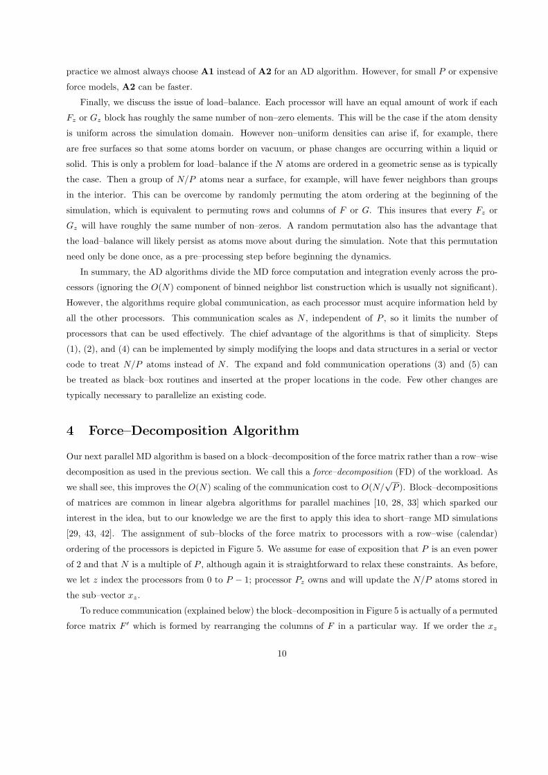
4 Force–Decomposition Algorithm

Our next parallel MD algorithm is based on a block–decomposition of the force matrix rather than a row–wise

decomposition as used in the previous section. We call this a force–decomposition (FD) of the workload. As

we shall see, this improves the O(N) scaling of the communication cost to O(N/√

P ). Block–decompositions

of matrices are common in linear algebra algorithms for parallel machines [10, 28, 33] which sparked our

interest in the idea, but to our knowledge we are the first to apply this idea to short–range MD simulations

[29, 43, 42]. The assignment of sub–blocks of the force matrix to processors with a row–wise (calendar)

ordering of the processors is depicted in Figure 5. We assume for ease of exposition that P is an even power

of 2 and that N is a multiple of P , although again it is straightforward to relax these constraints. As before,

we let z index the processors from 0 to P − 1; processor Pz owns and will update the N/P atoms stored in

the sub–vector xz.

To reduce communication (explained below) the block–decomposition in Figure 5 is actually of a permuted

force matrix F ′ which is formed by rearranging the columns of F in a particular way. If we order the xz

10

pieces in row–order, they form the usual position vector x which is shown as a vertical bar at the left of

the figure. Were we to have x span the columns as in Figure 1, we would form the force matrix as before.

Instead, we span the columns with a permuted position vector x′, shown as a horizontal bar at the top of

Figure 5, in which the xz pieces are stored in column–order. Thus, in the 16–processor example shown in

the figure, x stores each processor’s piece in the usual order (0, 1, 2, 3, 4, ..., 14, 15) while x′ stores them as

(0, 4, 8, 12, 1, 5, 9, 13, 2, 6, 10, 14, 3, 7, 11, 15). Now the (ij) element of F ′ is the force on atom i in vector x

due to atom j in permuted vector x′.

The F ′z sub–block owned by each processor Pz is of size (N/

√P ) × (N/

√P ). To compute the matrix

elements in F ′z, processor Pz must know one N/

√P–length piece of each of the x and x′ vectors, which

we denote as xα and x′β . As these elements are computed they will be accumulated into corresponding

force sub–vectors fα and f ′β . The Greek subscripts α and β each run from 0 to√

P − 1 and reference the

row and column position occupied by processor Pz. Thus for processor 6 in the figure, xα consists of the x

sub–vectors (4, 5, 6, 7) and x′β consists of the x′ sub–vectors (2, 6, 10, 14).

Our first FD algorithm F1 is outlined in Figure 6. As before, each processor has updated copies of the

needed atom positions xα and x′β at the beginning of the timestep. In step (1) neighbor lists are constructed.

Again, for small problems this is most quickly done by checking all N2/P possible pairs in F ′z. For large

problems, the N/√

P atoms in x′β are binned, then the 27 surrounding bins of each atom in xα is checked.

The total number of interactions stored in each processor’s lists is still O(N/P ). The scaling of the binned

neighbor list construction is thus N/P + N/√

P . In step (2) the neighbor lists are used to compute the

matrix elements in F ′z. As before the elements are summed into a local copy of fα as they are computed,

so F ′z never need be stored in matrix form. In step (3) a fold operation is performed within each row of

processors so that processor Pz obtains the total forces fz on its N/P atoms. Although the fold algorithm

used is the same as in the preceding section, there is a key difference. In this case the vector fα being folded

is only of length N/√

P and only the√

P processors in one row are participating in the fold. Thus this

operation scales as N/√

P instead of N as in the AD algorithm.

In step (4), fz is used by Pz to update the N/P atom positions in xz. Steps (5a-5b) share these updated

positions with all the processors that will need them for the next timestep. These are the processors which

share a row or column with Pz. First, in (5a), the processors in row α perform an expand of their xz

sub–vectors so that each acquires the entire xα. As with the fold, this operation scales as the N/√

P length

of xα instead of as N as it did in algorithms A1 and A2. Similarly, in step (5b), the processors in each

column β perform an expand of their xz. As a result they all acquire x′β and are ready to begin the next

timestep.

It is in step (5) that using a permuted force matrix F ′ saves extra communication. The permuted form

of F ′ causes xz to be a component of both xα and x′β for each Pz. This would not be the case if we had

block–decomposed the original force matrix F by having x span the columns instead of x′. Then in Figure 5

the xβ for P6 would have consisted of the sub–vectors (8, 9, 10, 11), none of which components are known by

11

P6. Thus, before performing the expand in step (5b), processor 6 would need to first acquire one of these 4

components from another processor (in the transpose position in the matrix [29]), requiring an extra O(N/P )

communication step. The transpose–free version of the FD algorithms presented here was motivated by a

matrix permutation for parallel matrix–vector multiplication discussed in reference [33].

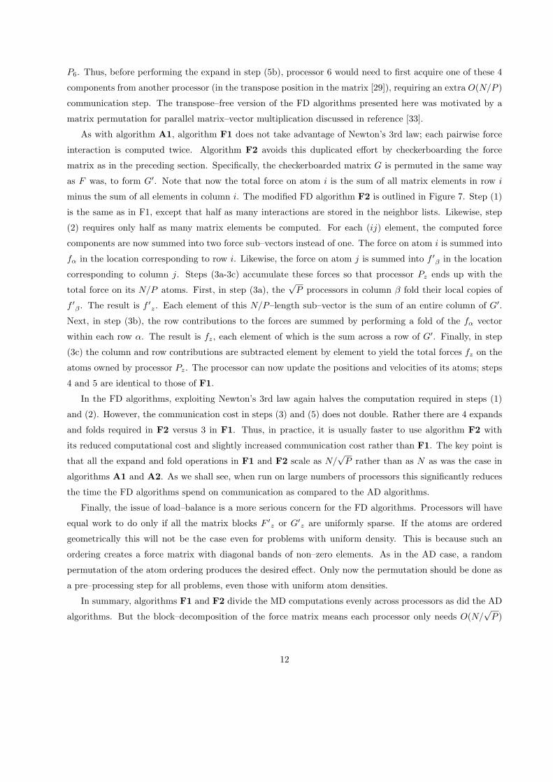
As with algorithm A1, algorithm F1 does not take advantage of Newton’s 3rd law; each pairwise force

interaction is computed twice. Algorithm F2 avoids this duplicated effort by checkerboarding the force

matrix as in the preceding section. Specifically, the checkerboarded matrix G is permuted in the same way

as F was, to form G′. Note that now the total force on atom i is the sum of all matrix elements in row i

minus the sum of all elements in column i. The modified FD algorithm F2 is outlined in Figure 7. Step (1)

is the same as in F1, except that half as many interactions are stored in the neighbor lists. Likewise, step

(2) requires only half as many matrix elements be computed. For each (ij) element, the computed force

components are now summed into two force sub–vectors instead of one. The force on atom i is summed into

fα in the location corresponding to row i. Likewise, the force on atom j is summed into f ′β in the location

corresponding to column j. Steps (3a-3c) accumulate these forces so that processor Pz ends up with the

total force on its N/P atoms. First, in step (3a), the√

P processors in column β fold their local copies of

f ′β . The result is f ′z. Each element of this N/P–length sub–vector is the sum of an entire column of G′.

Next, in step (3b), the row contributions to the forces are summed by performing a fold of the fα vector

within each row α. The result is fz, each element of which is the sum across a row of G′. Finally, in step

(3c) the column and row contributions are subtracted element by element to yield the total forces fz on the

atoms owned by processor Pz. The processor can now update the positions and velocities of its atoms; steps

4 and 5 are identical to those of F1.

In the FD algorithms, exploiting Newton’s 3rd law again halves the computation required in steps (1)

and (2). However, the communication cost in steps (3) and (5) does not double. Rather there are 4 expands

and folds required in F2 versus 3 in F1. Thus, in practice, it is usually faster to use algorithm F2 with

its reduced computational cost and slightly increased communication cost rather than F1. The key point is

that all the expand and fold operations in F1 and F2 scale as N/√

P rather than as N as was the case in

algorithms A1 and A2. As we shall see, when run on large numbers of processors this significantly reduces

the time the FD algorithms spend on communication as compared to the AD algorithms.

Finally, the issue of load–balance is a more serious concern for the FD algorithms. Processors will have

equal work to do only if all the matrix blocks F ′z or G′

z are uniformly sparse. If the atoms are ordered

geometrically this will not be the case even for problems with uniform density. This is because such an

ordering creates a force matrix with diagonal bands of non–zero elements. As in the AD case, a random

permutation of the atom ordering produces the desired effect. Only now the permutation should be done as

a pre–processing step for all problems, even those with uniform atom densities.

In summary, algorithms F1 and F2 divide the MD computations evenly across processors as did the AD

algorithms. But the block–decomposition of the force matrix means each processor only needs O(N/√

P )

12

information to perform its computations. Thus the communication and memory costs are reduced by a

factor of√

P versus algorithms A1 and A2. The FD strategy retains the simplicity of the AD technique;

F1 and F2 can be implemented using the same “black–box” communication routines as A1 and A2. The

FD algorithms also need no geometric information about the physical problem being modeled to perform

optimally. In fact, for load–balancing purposes the algorithms intentionally ignore such information by using

a random atom ordering.

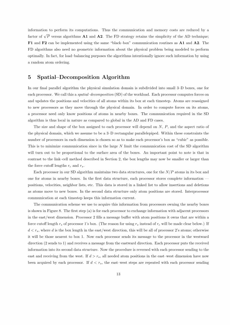
5 Spatial–Decomposition Algorithm

In our final parallel algorithm the physical simulation domain is subdivided into small 3–D boxes, one for

each processor. We call this a spatial–decomposition (SD) of the workload. Each processor computes forces on

and updates the positions and velocities of all atoms within its box at each timestep. Atoms are reassigned

to new processors as they move through the physical domain. In order to compute forces on its atoms,

a processor need only know positions of atoms in nearby boxes. The communication required in the SD

algorithm is thus local in nature as compared to global in the AD and FD cases.

The size and shape of the box assigned to each processor will depend on N , P , and the aspect ratio of

the physical domain, which we assume to be a 3–D rectangular parallelepiped. Within these constraints the

number of processors in each dimension is chosen so as to make each processor’s box as “cubic” as possible.

This is to minimize communication since in the large N limit the communication cost of the SD algorithm

will turn out to be proportional to the surface area of the boxes. An important point to note is that in

contrast to the link–cell method described in Section 2, the box lengths may now be smaller or larger than

the force cutoff lengths rc and rs.

Each processor in our SD algorithm maintains two data structures, one for the N/P atoms in its box and

one for atoms in nearby boxes. In the first data structure, each processor stores complete information —

positions, velocities, neighbor lists, etc. This data is stored in a linked list to allow insertions and deletions

as atoms move to new boxes. In the second data structure only atom positions are stored. Interprocessor

communication at each timestep keeps this information current.

The communication scheme we use to acquire this information from processors owning the nearby boxes

is shown in Figure 8. The first step (a) is for each processor to exchange information with adjacent processors

in the east/west dimension. Processor 2 fills a message buffer with atom positions it owns that are within a

force cutoff length rs of processor 1’s box. (The reason for using rs instead of rc will be made clear below.) If

d < rs, where d is the box length in the east/west direction, this will be all of processor 2’s atoms; otherwise

it will be those nearest to box 1. Now each processor sends its message to the processor in the westward

direction (2 sends to 1) and receives a message from the eastward direction. Each processor puts the received

information into its second data structure. Now the procedure is reversed with each processor sending to the

east and receiving from the west. If d > rs, all needed atom positions in the east–west dimension have now

been acquired by each processor. If d < rs, the east–west steps are repeated with each processor sending

13

more needed atom positions to its adjacent processors. For example, processor 2 sends processor 1 atom

positions from box 3 (which processor 2 now has in its second data structure). This can be repeated until

each processor knows all atom positions within a distance rs of its box, as indicated by the dotted boxes in

the figure. The same procedure is now repeated in the north/south dimension; see step (b) of the figure.

The only difference is that messages sent to the adjacent processor now contain not only atoms the processor

owns (in its first data structure), but also any atom positions in its second data structure that are needed

by the adjacent processor. For d = rs this has the effect of sending 3 boxes worth of atom positions in one

message as shown in (b). Finally, in step (c) the process is repeated in the up/down dimension. Now atom

positions from an entire plane of boxes (9 in the figure) are being sent in each message.

There are several key advantages to this scheme, all of which reduce the overall cost of communication

in our algorithm. First, for d ≥ rs, needed atom positions from all 26 surrounding boxes are obtained in

just 6 data exchanges. Moreover, as will be discussed in Section 7, if the parallel machine is a hypercube,

the processors can be mapped to the boxes in such a way that all 6 of these processors will be directly

connected to the center processor. Thus message passing will be fast and contention–free. Second, when

d < rs so that atom information is needed from more distant boxes, this occurs with only a few extra data

exchanges, all of which are still with the 6 immediate neighbor processors. This is an important feature of

the algorithm which enables it to perform well even when large numbers of processors are used on relatively

small problems.

A third advantage is that the amount of data communicated is minimized. Each processor acquires only

the atom positions that are within a distance rs of its box. Fourth, all of the received atom positions can be

placed as contiguous data directly into the processor’s second data structure. No time is spent rearranging

data, except to create the buffered messages that need to be sent. Finally, as will be discussed in more detail

below, this message creation can be done very quickly. A full scan of the two data structures is only done

once every few timesteps, when the neighbor lists are created, to decide which atom positions to send in

each message. The scan procedure creates a list of atoms that make up each message. During all the other

timesteps, the lists can be used, in lieu of scanning the full atom list, to directly index the referenced atoms

and buffer up the messages quickly. This is the equivalent of a gather operation on a vector machine.

We now outline our SD algorithm S1 in Figure 9. Box z is assigned to processor Pz, where z runs from

0 to P − 1 as before. Processor Pz stores the atom positions of its N/P atoms in xz and the forces on those

atoms in fz. Steps (1a-1c) are the neighbor list construction, performed once every few timesteps. This is

somewhat more complex than in the other algorithms because, as discussed above, it includes the creation

of lists of atoms that will be communicated at every timestep. First, in step (1a) the positions, velocities,

and any other identifying information of atoms that are no longer inside box z are deleted from xz (first

data structure) and stored in a message buffer. These atoms are exchanged with the 6 adjacent processors

via the communication pattern of Figure 8. As the information routes through each dimension, processor

Pz checks for new atoms that are now inside its box boundaries, adding them to its xz. Next, in step (1b),

14

all atom positions within a distance rs of box z are acquired by the communication scheme described above.

As the different messages are buffered by scanning through the two data structures, lists of included atoms

are made. The lists will be used in step (5). The scaling factor ∆ for steps (1a) and (1b) will be explained

below.

When steps (1a) and (1b) are complete, both of the processor’s data structures are current. Neighbor

lists for its N/P atoms can now be constructed in step (1c). If atoms i and j are both in box z (an inner–box

interaction), the (ij) pair is only stored once in the neighbor list. If i and j are in different boxes (a two–box

interaction), both processors store the interaction in their respective neighbor lists. If this were not done,

processors would compute forces on atoms they do not own and communication of the forces back to the

processors owning the atoms would be required. A modified algorithm which performs this communication

to avoid the duplicated force computation of two–box interactions is discussed below. When d, the length of

box z, is less than two cutoff distances, it is quicker to find neighbor interactions by checking each atom inside

box z against all the atoms in both of the processor’s data structures. This scales as the square of N/P . If

d > 2rs, then with the shell of atoms around box z, there are 4 or more bins in each dimension. In this case,

as with the algorithms of the preceding sections, it is quicker to perform the neighbor list construction by

binning. All the atoms in both data structures are mapped to bins of size rs. The surrounding bins of each

atom in box z are then checked for possible neighbors.

Processor Pz can now compute all the forces on its atoms in step (2) using the neighbor lists. When

the interaction is between two atoms inside box z, the resulting force is stored twice in fz, once for atom

i and once for atom j. For two–box interactions, only the force on the processor’s own atom is stored.

After computing fz, the atom positions are updated in step (4). Finally, these updated positions must be

communicated to the surrounding processors in preparation for the next timestep. This occurs in step (5) in

the communication pattern of Figure 8 using the previously created lists. The amount of data exchanged in

this operation is a function of the relative values of the force cutoff distance and box length and is discussed

in the next paragraph. Also, we note that on the timesteps that neighbor lists are constructed, step (5) does

not have to be performed since step (1b) has the same effect.

The communication operations in algorithm S1 occur in steps (1a), (1b), and (5). The communication

in the latter two steps is identical. The cost of these steps scales as the volume of data exchanged. For step

(5), if we assume uniform atom density, this is proportional to the physical volume of the shell of thickness

rs around box z, namely (d + 2rs)3 − d3. Note there are roughly N/P atoms in a volume of d3, since d3 is

the size of box z. There are 3 cases to consider. First, if d < rs data from many neighboring boxes must

be exchanged and the operation scales as 8rs3. Second, if d ≈ rs, the data in all 26 surrounding boxes is

exchanged and the operation scales as 27N/P . Finally, if d is much larger than rs, only atom positions near

the 6 faces of box z will be exchanged. The communication then scales as the surface area of box z, namely

6rs(N/P )2/3. These 3 cases are explicitly listed in the scaling of step (5). Elsewhere in Figure 9, we use the

term ∆ to represent whichever of the three is applicable for a given N , P , and rs. We note that step (1a)

15

involves less communication since not all the atoms within a cutoff distance of a box face will move out of

the box. But this operation still scales as the surface area of box z, so we list its scaling as ∆.

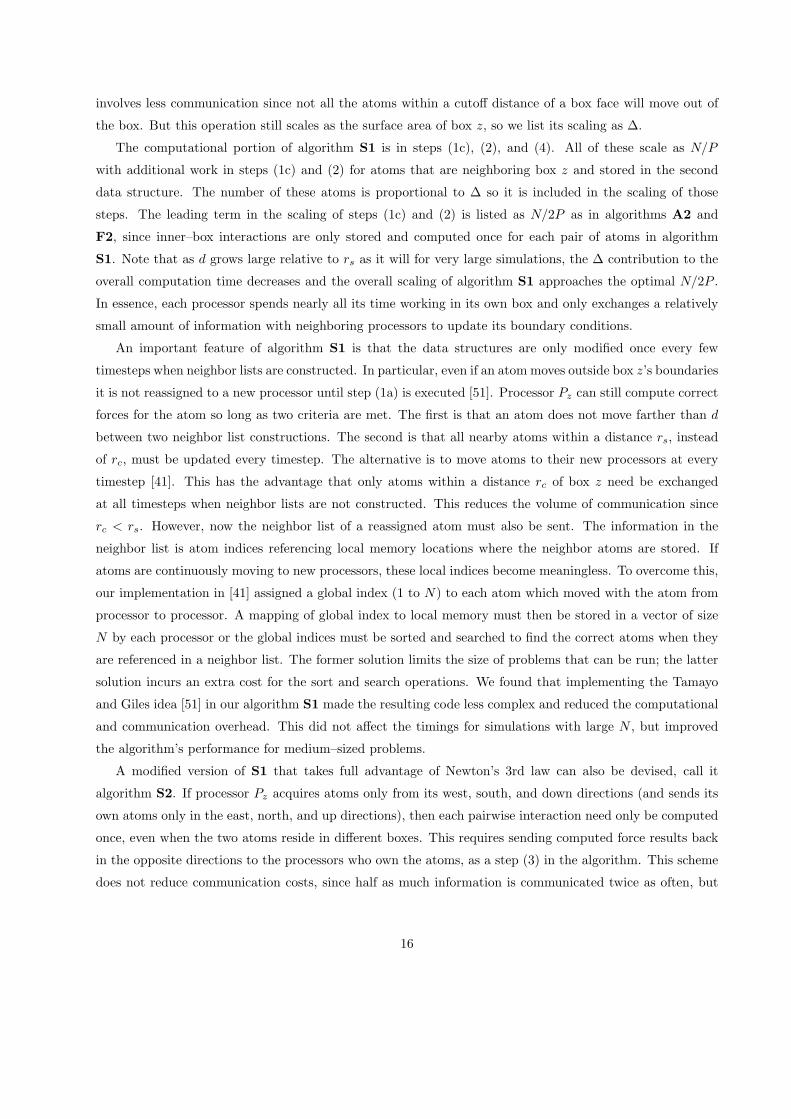
The computational portion of algorithm S1 is in steps (1c), (2), and (4). All of these scale as N/P

with additional work in steps (1c) and (2) for atoms that are neighboring box z and stored in the second

data structure. The number of these atoms is proportional to ∆ so it is included in the scaling of those

steps. The leading term in the scaling of steps (1c) and (2) is listed as N/2P as in algorithms A2 and

F2, since inner–box interactions are only stored and computed once for each pair of atoms in algorithm

S1. Note that as d grows large relative to rs as it will for very large simulations, the ∆ contribution to the

overall computation time decreases and the overall scaling of algorithm S1 approaches the optimal N/2P .

In essence, each processor spends nearly all its time working in its own box and only exchanges a relatively

small amount of information with neighboring processors to update its boundary conditions.

An important feature of algorithm S1 is that the data structures are only modified once every few

timesteps when neighbor lists are constructed. In particular, even if an atom moves outside box z’s boundaries

it is not reassigned to a new processor until step (1a) is executed [51]. Processor Pz can still compute correct

forces for the atom so long as two criteria are met. The first is that an atom does not move farther than d

between two neighbor list constructions. The second is that all nearby atoms within a distance rs, instead

of rc, must be updated every timestep. The alternative is to move atoms to their new processors at every

timestep [41]. This has the advantage that only atoms within a distance rc of box z need be exchanged

at all timesteps when neighbor lists are not constructed. This reduces the volume of communication since

rc < rs. However, now the neighbor list of a reassigned atom must also be sent. The information in the

neighbor list is atom indices referencing local memory locations where the neighbor atoms are stored. If

atoms are continuously moving to new processors, these local indices become meaningless. To overcome this,

our implementation in [41] assigned a global index (1 to N) to each atom which moved with the atom from

processor to processor. A mapping of global index to local memory must then be stored in a vector of size

N by each processor or the global indices must be sorted and searched to find the correct atoms when they

are referenced in a neighbor list. The former solution limits the size of problems that can be run; the latter

solution incurs an extra cost for the sort and search operations. We found that implementing the Tamayo

and Giles idea [51] in our algorithm S1 made the resulting code less complex and reduced the computational

and communication overhead. This did not affect the timings for simulations with large N , but improved

the algorithm’s performance for medium–sized problems.

A modified version of S1 that takes full advantage of Newton’s 3rd law can also be devised, call it

algorithm S2. If processor Pz acquires atoms only from its west, south, and down directions (and sends its

own atoms only in the east, north, and up directions), then each pairwise interaction need only be computed

once, even when the two atoms reside in different boxes. This requires sending computed force results back

in the opposite directions to the processors who own the atoms, as a step (3) in the algorithm. This scheme

does not reduce communication costs, since half as much information is communicated twice as often, but

16

does eliminate the duplicated force computations for two–box interactions. An algorithm similar to this is

detailed in [14] for the Fujitsu AP1000 machine with results that we highlight in the next section. Two

points are worth noting. First, the overall savings of S2 over S1 is small, particularly for large N . Only

the ∆ term in steps (1c) and (2) is saved. Second, as we will show in Section 7, the performance of SD

algorithms for large systems can be improved by optimizing the single–processor force computation in step

(2). As with vector machines this requires more attention be paid to data structures and loop orderings in

the force and neighbor–list construction routines to achieve high single–processor flop rates. Implementing

S2 requires special–case coding for atoms near box edges and corners to insure all interactions are counted

only once [14] which can hinder this optimization process.

Finally, the issue of load–balance is an important concern in any SD algorithm. Algorithm S1 will be load–

balanced only if all boxes have a roughly equal number of atoms (and surrounding atoms). This will not be

the case if the physical atom density is non–uniform. Additionally, if the physical domain is not a rectangular

parallelepiped, it can be difficult to split into P equal–sized pieces. Sophisticated load–balancing algorithms

have been developed [27] to partition an irregular physical domain or non–uniformly dense clusters of atoms,

but they create sub–domains which are irregular in shape or are connected in an irregular fashion to their

neighboring sub–domains. In either case, the task of assigning atoms to sub–domains and communicating

with neighbors becomes more costly and complex. If the physical atom density changes over time during

the MD simulation, the load–balance problem is compounded. Any dynamic load–balancing scheme requires

additional computational overhead and data movement.

In summary, the SD algorithm, like the AD and FD algorithms, evenly divides the MD computations

across all the processors. Its chief benefit is that it takes full advantage of the local nature of the interatomic

forces by performing only local communication. Thus, in the large N limit, it achieves optimal O(N/P )

scaling and is clearly the fastest algorithm. However, this is only true if good load–balance is also achievable.

Since its performance is sensitive to the problem geometry, algorithm S1 is more restrictive than A2 and

F2 whose performance is geometry–independent. A second drawback of algorithm S1 is its complexity;

it is more difficult to implement efficiently than the simpler AD and FD algorithms. In particular the

communication scheme requires extra coding and bookkeeping to create messages and access data received

from neighboring boxes. In practice, integrating algorithm S1 into an existing serial MD code can require a

substantial reworking of data structures and code.

6 Benchmark Problem

The test case used to benchmark our three parallel algorithms is a MD problem that has been used extensively

by various researchers [9, 14, 20, 24, 30, 41, 47, 51, 52]. It models atom interactions with a Lennard–Jones

potential energy between pairs of atoms separated by a distance r as

17

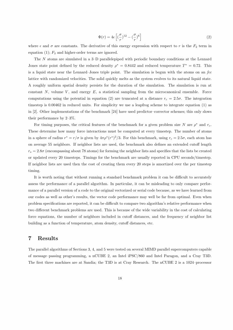
Φ(r) = 4ε[(σ

r)12 − (

σ

r)6

](2)

where ε and σ are constants. The derivative of this energy expression with respect to r is the F2 term in

equation (1); F3 and higher-order terms are ignored.

The N atoms are simulated in a 3–D parallelepiped with periodic boundary conditions at the Lennard

Jones state point defined by the reduced density ρ∗ = 0.8442 and reduced temperature T ∗ = 0.72. This

is a liquid state near the Lennard–Jones triple point. The simulation is begun with the atoms on an fcc

lattice with randomized velocities. The solid quickly melts as the system evolves to its natural liquid state.

A roughly uniform spatial density persists for the duration of the simulation. The simulation is run at

constant N , volume V , and energy E, a statistical sampling from the microcanonical ensemble. Force

computations using the potential in equation (2) are truncated at a distance rc = 2.5σ. The integration

timestep is 0.00462 in reduced units. For simplicity we use a leapfrog scheme to integrate equation (1) as

in [2]. Other implementations of the benchmark [24] have used predictor–corrector schemes; this only slows

their performance by 2–3%.

For timing purposes, the critical features of the benchmark for a given problem size N are ρ∗ and rc.

These determine how many force interactions must be computed at every timestep. The number of atoms

in a sphere of radius r∗ = r/σ is given by 4πρ∗(r∗)3/3. For this benchmark, using rc = 2.5σ, each atom has

on average 55 neighbors. If neighbor lists are used, the benchmark also defines an extended cutoff length

rs = 2.8σ (encompassing about 78 atoms) for forming the neighbor lists and specifies that the lists be created

or updated every 20 timesteps. Timings for the benchmark are usually reported in CPU seconds/timestep.

If neighbor lists are used then the cost of creating them every 20 steps is amortized over the per timestep

timing.

It is worth noting that without running a standard benchmark problem it can be difficult to accurately

assess the performance of a parallel algorithm. In particular, it can be misleading to only compare perfor-

mance of a parallel version of a code to the original vectorized or serial code because, as we have learned from

our codes as well as other’s results, the vector code performance may well be far from optimal. Even when

problem specifications are reported, it can be difficult to compare two algorithm’s relative performance when

two different benchmark problems are used. This is because of the wide variability in the cost of calculating

force equations, the number of neighbors included in cutoff distances, and the frequency of neighbor list

building as a function of temperature, atom density, cutoff distances, etc.

7 Results

The parallel algorithms of Sections 3, 4, and 5 were tested on several MIMD parallel supercomputers capable

of message–passing programming, a nCUBE 2, an Intel iPSC/860 and Intel Paragon, and a Cray T3D.

The first three machines are at Sandia; the T3D is at Cray Research. The nCUBE 2 is a 1024–processor

18

hypercube. Each processor is a custom scalar chip capable of about 2 Mflops peak and has 4 Gbytes of

memory. The communications bandwidth between processors is 2 Mbytes/sec. Sandia’s iPSC/860 has 64

i860XR processors connected in a hypercube topology. Its processors have 8 Mbytes of memory and are

capable of about 60 Mflops peak, but in practice 4–7 Mflops is the typical compiled Fortran performance.

Communications bandwidth on the iPSC/860 is 2.7 Mbytes/sec. The Intel Paragon at Sandia has from 1840

to 1904 processors which are connected as a 2–D mesh. The individual i860XP processors have 16 Mbytes of

memory and are about 30% faster than those in the iPSC/860. The Paragon communication bandwidth is

150 Mbytes/sec peak, but in practice is a function of message length and data alignment. The Cray T3D used

in this study has 512 processors connected as a 3–D torus, each with 64 Mbytes of memory. Its processors are

DEC Alpha (RISC) chips capable of 150 Mflops peak with typical compiled Fortran performance of 15–20

Mflops. The T3D communications bandwidth is 165 Mbytes/sec peak.

Because the algorithms were implemented in standard Fortran with calls to vendor–supplied message–

passing subroutines (sends and receives), only minor changes were required to implement the benchmark

codes on the different machines. As described, the algorithms do not specify a mapping of physical processors

to logical computational elements (force matrix sub–blocks, 3–D boxes). An optimal mapping would be

tailored to a particular machine architecture so as to minimize message contention (multiple messages using

the same communication wire) and the distance messages have to travel between pairs of processors that are

not directly connected by a communication wire. The mappings we use are near–optimal and conceptually

simple.

For the atom–decomposition (AD) algorithm we simply assign the processors in ascending order to the

row–blocks of the force matrix as in Figure 1. The expands and folds then take place exactly as in Figure

2. On the hypercube machines (nCUBE and iPSC/860) this is optimal; on the mesh machines (Paragon

and T3D) some messages will (unavoidably) be exchanged between non–neighbor processors. For the force–

decomposition (FD) algorithm we use a natural calendar ordering of the processors in the permuted force

matrix as in Figure 5. On a hypercube this means each row and column of the matrix is a sub–cube of

processors so that expands and folds within rows and columns can be done optimally. On a 2–D mesh

(Paragon), all the communication is within rows and columns of processors, until we use so many processors

that (for example) 16x64 physical processors are configured as a 32x32 logical mesh.

For the spatial–decomposition (SD) algorithm on the hypercube machines we use a processor mapping

that configures the hypercube as a 3–D torus. Such a mapping is done using a Gray–coded ordering [22]

of the processors. This insures each processor’s box in Figure 8 has 6 spatial neighbors (boxes in the east,

west, north, south, up, down directions) that are assigned to processors which are also nearest neighbors

in the hypercube topology. Communication with these neighbors is thus contention–free. Gray–coding also

provides naturally for periodic boundary conditions in the MD simulation since processors at the edge of

the 3–D torus are topological nearest neighbors to those on the opposite edge. On the Paragon we assign

planes of boxes in the 3–D domain to contiguous subsets of the 2–D mesh of processors; data exchanges in

19

the 3rd dimension thus (unavoidably) require non–nearest–neighbor communication. On the Cray T3D the

physical 3–d domain maps naturally to the 3–d torus of processors.

Timing results for the benchmark problem on the different parallel machines are shown in Tables I, II, and

III for the AD, FD, and SD algorithms. A wide range of problem sizes are considered from N = 500 atoms

to N = 108 atoms. The lattice size for each problem is also specified; there are 4 atoms per unit cell for the

initial–state fcc lattices. Entries with a dashed line are for problems that would not fit in available memory.

The 100,000,000 atom problem nearly filled the 30 Gbytes of memory on the 1904–processor Paragon with

neighbor lists consuming the majority of the space.

For comparison, we also implemented the vectorized algorithm of Grest, et al. [24] on single processors

of Sandia’s Cray Y–MP and a Cray C90 at Cray Research. Our version is only slightly different from the

original Grest code, using a simpler integrator and allowing for non–cubic physical domains. The timings in

reference [24] were for a Cray X–MP. We believe these timings for the faster Y–MP and C90 architectures

are the fastest that have been reported for this benchmark problem on a single processor of a conventional

vector supercomputer. They show a C90 processor to be about 2.5 times faster than a Y–MP processor

for this algorithm. The starred Cray timings in the tables are estimates for problems too large to fit in

memory on the machines accessible to us. They are extrapolations of the N = 105 system timing based on

the observed linear scaling of the Cray algorithm. It is also worth noting that ideas similar to those used

in the parallel algorithms of the previous sections could be used to create efficient parallel Cray codes for

multiple processors of a Y–MP or C90. For example, a speed–up of 6.8 on a 8–processor Cray Y–MP has

been achieved by Attig and Kremer with the Grest, et al. algorithm [3].

Finally, we have also implemented specially optimized versions of the SD algorithm on the Intel Paragon.

Performance numbers for these codes are shown in Table IV. The first enhancement takes advantage of the

fact that each “node” of the Paragon actually has two i860 processors, one for computation and one for

communication. An option under the SUNMOS operating system [35] run on Sandia’s Paragon is to use

the second processor for computation. This requires minor coding changes to stride the loops in the force

and neighbor routines so that each processor can perform independent computations (without writing to

the same memory location) simultaneously. The speed-up due to this enhancement is less than a factor of

two, since both processors are competing for bus bandwidth to memory. The second enhancement was more

work; it involved writing an i860 assembler version (see acknowledgments) of the most critical computational

kernel, the force computation, which takes 70 to 80% of the time for large problems. The assembler routine

is about 2.5 times faster than its Fortran counterpart, yielding an overall speed–up of about 1.75 on large

problems. These enhancements can be combined (minus an overhead factor due to bus competition) to yield

the fastest version of the code with a speed–up of nearly 3 over the original Fortran code.

The parallel timings in all of the tables for the nCUBE and Intel machines are for single–precision (32–

bit) implementations of the benchmark. The Y–MP, C90, and T3D timings are for 64–bit arithmetic since

that is the only option. MD simulations do not typically require double precision accuracy since there is a

20

Table I: CPU seconds/timestep for the atom–decomposition algorithm A1 on several parallel machines for

the benchmark simulation. Single processor Cray Y–MP and C90 timings using a fully vectorized algorithm

are also given for comparison.

much coarser approximation inherent in the potential model and the integrator. This is particularly true

of Lennard–Jones systems since the ε and σ coefficients are only specified to a few digits of accuracy as an

approximate model of the interatomic energies in a real material. With this said, double precision timings

can be easily estimated. The processors in the nCUBE and Intel machines compute about 20–30% slower in

double–precision arithmetic than single, so the time spent computing would be increased by that amount.

Communication costs in each of the algorithms would essentially double, since the volume of information

being exchanged in messages would increase by a factor of two. Thus depending on the fraction of time

being spent in communication for a particular N and P (see the scaling discussion below), the overall

timings typically increase by 20–50% for double–precision runs.

The tables show the parallel machines to be competitive with the Cray Y–MP and C90 machines across

the entire range of problem sizes for all three parallel algorithms. The FD algorithm is fastest for the smallest

problem sizes; SD is fastest for large N . For the Fortran version of the code the Cray T3D is the fastest of the

parallel machines on a per–processor basis; overall the Intel Paragon is the fastest. On 1840 dual–processor

nodes of the Paragon (3680 i860 processors) the assembler–optimized SD code is 415 times faster than a

21

Table II: CPU seconds/timestep for the force–decomposition algorithm F2 on several parallel machines and

the Cray Y–MP and C90.

single Y–MP processor on the largest problem sizes and 165 times faster than a C90 processor. A surprising

result is that the parallel machines are competitive with a single processor of the Cray machines even for

the smallest problem sizes. One typically does not think of there being enough parallelism to exploit when

there are only a few atoms per processor.

The floating point operation (flop) rate for the parallel codes can also be estimated. Computing the

force between two interacting atoms requires 23 flops with an average of 27.6 interactions per atom (taking

into account Newton’s 3rd law) computed each timestep for the benchmark. This gives a total flop rate

for the Fortran code of 6.97 Gflops for the 100,000,000 atom problem on 1904 processors of the Paragon.

The dual–processor assembler–optimized version runs the same problem at 18.0 Gflops on 1840 nodes. By

comparison the C90 processor is running at 107 Mflops for large N though its hardware performance monitor

reports a rate of over 200 Mflops. The difference is that both the vector and parallel codes perform flops

to set up neighbor lists and check atom distances that end up outside the force cutoff; we are not counting

them in these figures since they do not contribute to the answer.

Large N timings for this benchmark on other parallel machines are discussed in [9, 14, 20, 52], all for

SD algorithms. The best timings on SIMD machines are reported by Tamayo, et al. [52] who implemented

22

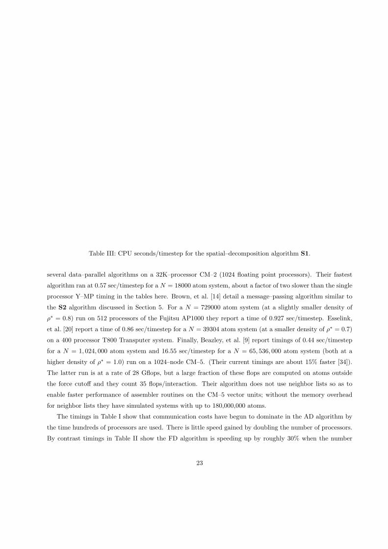
Table III: CPU seconds/timestep for the spatial–decomposition algorithm S1.

several data–parallel algorithms on a 32K–processor CM–2 (1024 floating point processors). Their fastest

algorithm ran at 0.57 sec/timestep for a N = 18000 atom system, about a factor of two slower than the single

processor Y–MP timing in the tables here. Brown, et al. [14] detail a message–passing algorithm similar to

the S2 algorithm discussed in Section 5. For a N = 729000 atom system (at a slightly smaller density of

ρ∗ = 0.8) run on 512 processors of the Fujitsu AP1000 they report a time of 0.927 sec/timestep. Esselink,

et al. [20] report a time of 0.86 sec/timestep for a N = 39304 atom system (at a smaller density of ρ∗ = 0.7)

on a 400 processor T800 Transputer system. Finally, Beazley, et al. [9] report timings of 0.44 sec/timestep

for a N = 1, 024, 000 atom system and 16.55 sec/timestep for a N = 65, 536, 000 atom system (both at a

higher density of ρ∗ = 1.0) run on a 1024–node CM–5. (Their current timings are about 15% faster [34]).

The latter run is at a rate of 28 Gflops, but a large fraction of these flops are computed on atoms outside

the force cutoff and they count 35 flops/interaction. Their algorithm does not use neighbor lists so as to

enable faster performance of assembler routines on the CM–5 vector units; without the memory overhead

for neighbor lists they have simulated systems with up to 180,000,000 atoms.

The timings in Table I show that communication costs have begun to dominate in the AD algorithm by

the time hundreds of processors are used. There is little speed gained by doubling the number of processors.

By contrast timings in Table II show the FD algorithm is speeding up by roughly 30% when the number

23

of processors is doubled. The timings for the largest problem sizes in Table III evidence excellent scaling

properties even on relatively small problems when there are only a few atoms per processor. Doubling

P nearly halves the run times for a given N . Similarly, as N increases for fixed P , the run times per

atom actually become faster as the surface–to–volume ratio of each processor’s box is reduced. We note,

however, that this scaling depends on uniform atom density within a simple domain such as the rectangular

parallelepiped of the benchmark problem.

The algorithm’s relative performance can be better seen in graphical form using data from all 3 tables.

Figure 10 shows a 1024–processor Paragon’s performance on the benchmark simulation as a function of

problem size. Single processor Y–MP and C90 timings are also included. The linear scaling of all the

algorithms in the large N limit is evident. Note that FD is faster than AD across all problem sizes due to

its reduced communication costs. On this many processors, the SD algorithm has significant overhead costs

for small N . This is because the d/rs ratio is so small that each processor has to communicate with a large

number of neighboring processors to acquire all its needed information. As N increases, this overhead is

reduced relative to the computation performed inside the processor’s box, and the algorithm’s performance

asymptotically approaches its optimal O(N/P ) performance. Thus there is a cross–over size N at which the

SD algorithm becomes faster than FD. For this benchmark it is at about 4 atoms/processor indicating that

the spatial algorithm is still working quite well even when the box size is small relative to the force cutoff.

In Figure 11 we plot the nCUBE 2’s performance on the N = 10976 atom benchmark as a function of

number of processors for two different cutoff lengths, 2.5σ (solid symbols) and 5.0σ (open symbols). Single

processor Y–MP and C90 timings are also shown for the 2.5σ benchmark. The dotted lines are the maximum

achievable speed of the nCUBE if any of the algorithms were 100% efficient. Parallel efficiency is defined as

the run time on 1 processor divided by the quantity (P×run time on P processors). Thus if the 512–processor

timing is 256 times as fast as the 1–processor timing, the algorithm is 50% efficient. On small numbers of

processors communication is not a significant factor and all the algorithms perform similarly; as P increases,

the algorithms become less efficient. The AD algorithm falls off most rapidly due to the O(N) scaling of its

communication. For the 2.5σ case, FD is next most efficient due to its O(N/√

P ) communication scaling.

When hundreds of processors are used, even the SD algorithm becomes less efficient since now the box size is

small relative to the force cutoff distance for this N . For the longer cutoff case (more typical of what might

be used in an organic system simulation with Coulombic forces), the FD algorithm is actually faster than

SD for all P . This is because the communication cost in the AD and FD algorithms is independent of the

cutoff length, unlike the SD case.

Using one–processor timings as reference points, parallel efficiencies can be computed for all the algorithms

or, equivalently, the fraction of time spent in communication in each of the entries in Tables I, II, and III.

Running the largest problems that fit in memory on a single processor of each of the parallel machines gave

timings on the Cray T3D, nCUBE 2, and Intel iPSC/860 and Paragon of 8.23×10−5, 9.15×10−4, 2.03×10−4,

and 1.57× 10−4 seconds/timestep/atom respectively. By comparison, single–processor Cray Y–MP and C90

24

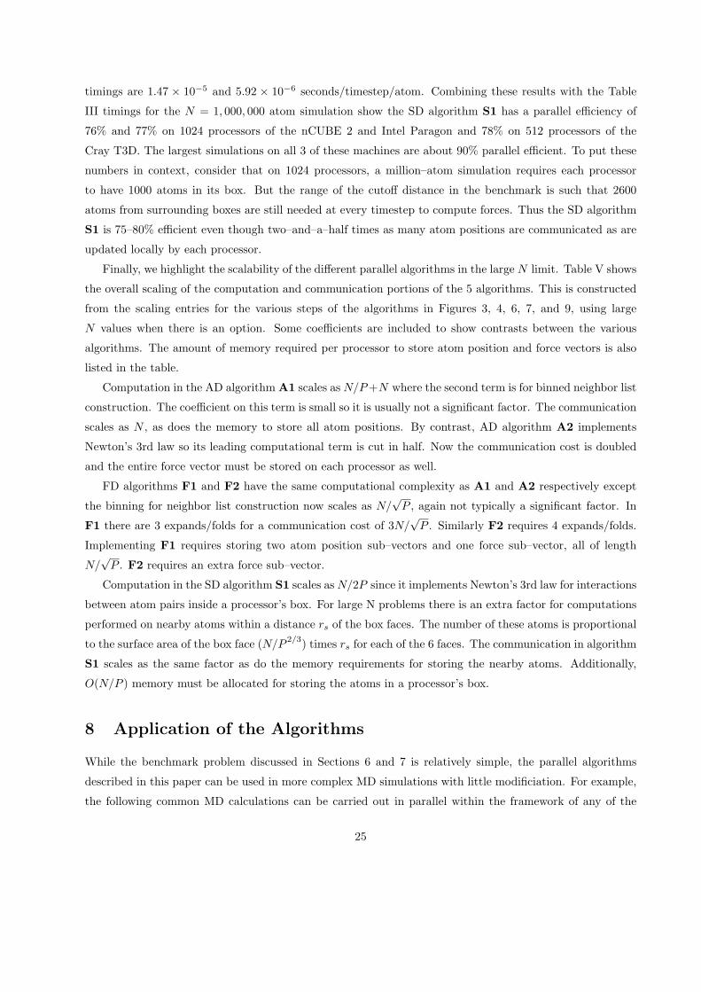
timings are 1.47 × 10−5 and 5.92 × 10−6 seconds/timestep/atom. Combining these results with the Table

III timings for the N = 1, 000, 000 atom simulation show the SD algorithm S1 has a parallel efficiency of

76% and 77% on 1024 processors of the nCUBE 2 and Intel Paragon and 78% on 512 processors of the

Cray T3D. The largest simulations on all 3 of these machines are about 90% parallel efficient. To put these

numbers in context, consider that on 1024 processors, a million–atom simulation requires each processor

to have 1000 atoms in its box. But the range of the cutoff distance in the benchmark is such that 2600

atoms from surrounding boxes are still needed at every timestep to compute forces. Thus the SD algorithm

S1 is 75–80% efficient even though two–and–a–half times as many atom positions are communicated as are

updated locally by each processor.

Finally, we highlight the scalability of the different parallel algorithms in the large N limit. Table V shows

the overall scaling of the computation and communication portions of the 5 algorithms. This is constructed

from the scaling entries for the various steps of the algorithms in Figures 3, 4, 6, 7, and 9, using large

N values when there is an option. Some coefficients are included to show contrasts between the various

algorithms. The amount of memory required per processor to store atom position and force vectors is also

listed in the table.

Computation in the AD algorithm A1 scales as N/P +N where the second term is for binned neighbor list

construction. The coefficient on this term is small so it is usually not a significant factor. The communication

scales as N , as does the memory to store all atom positions. By contrast, AD algorithm A2 implements

Newton’s 3rd law so its leading computational term is cut in half. Now the communication cost is doubled

and the entire force vector must be stored on each processor as well.

FD algorithms F1 and F2 have the same computational complexity as A1 and A2 respectively except

the binning for neighbor list construction now scales as N/√

P , again not typically a significant factor. In

F1 there are 3 expands/folds for a communication cost of 3N/√

P . Similarly F2 requires 4 expands/folds.

Implementing F1 requires storing two atom position sub–vectors and one force sub–vector, all of length

N/√

P . F2 requires an extra force sub–vector.

Computation in the SD algorithm S1 scales as N/2P since it implements Newton’s 3rd law for interactions

between atom pairs inside a processor’s box. For large N problems there is an extra factor for computations

performed on nearby atoms within a distance rs of the box faces. The number of these atoms is proportional

to the surface area of the box face (N/P2/3) times rs for each of the 6 faces. The communication in algorithm

S1 scales as the same factor as do the memory requirements for storing the nearby atoms. Additionally,

O(N/P ) memory must be allocated for storing the atoms in a processor’s box.

8 Application of the Algorithms

While the benchmark problem discussed in Sections 6 and 7 is relatively simple, the parallel algorithms

described in this paper can be used in more complex MD simulations with little modificiation. For example,

the following common MD calculations can be carried out in parallel within the framework of any of the

25

3 algorithms: on–the–fly computation of thermodynamic quantities and transport coefficients, triggering

of neighbor list construction by atom movement, multiple–timescale methods [37, 50], more sophisticated

time integrators, and other statistical ensembles besides the constant NV E ensemble of the benchmark, e.g.

constant NPT simulations.

Virtually any form of short–range interatomic force function can be implemented within the AD or

SD framework. The FD algorithm is less general in this respect. If higher–order (3–body, 4–body, etc.)

interactions are included in the force model, one must insure some processor knows sufficient information to

compute any given interaction. An implementation for the embedded atom method (EAM) potentials [18]

used in modeling metals and metal alloys is discussed in [43] and a FD implementation of the many–body

forces (angular, torsional) encountered in molecular simulations is presented in [42]. We know of no simple

way to use the FD idea for the more general case of simulations with dynamically changing connectivities,

such as for silicon three–body potentials. Long–range pairwise forces can be computed directly with O(N2)

work in the force–matrix formalism of the AD and FD algorithms [29]. By contrast, the SD algorithm would

now require long–range communication and become inefficient.

In practical terms, how does one choose the “best” parallel algorithm for a particular MD simulation?

Assuming one knows the ranges of N and P the simulation will be run with, we find the following four

guidelines helpful.

(A) Choose an AD algorithm only if the communication cost is expected to be negligible. In this case

simplicity outweighs the inefficient communications. Typically this will only be true for small P (say P ≤ 16

processors) or very expensive forces where computation time dominates communication time.

(B) A FD approach will be faster than AD in all other cases. Both the AD and FD algorithms scale

linearly with N for fixed P . This means for a given P , the parallel efficiency of either algorithm is independent

of N . Moreover, as P doubles, the communication time in the AD algorithm is unchanged, while in the FD

algorithm it decreases by a factor of√

2. Thus, once P is large enough that FD is noticeably faster than

AD, it will remain faster as P increases, independent of N . For the benchmark problem this was the case

for P ≥ 16 processors.

(C) For a given P , the scaling of the SD algorithm is not linear with N . This is due to the fact each

proccessor’s box has volume d3 = N/P , but it computes and communicates information in an extended

volume of (d + 2rs)3, where rs is a neighbor list cutoff distance. For small N communication and overhead

costs are significant and the efficiency is poor; for large N the efficiency is asymptotically optimal (100%).

Thus when compared to a FD approach, there will be some cross–over point as N increases for a given

P where a SD algorithm becomes faster. In the benchmark the cross–over size was several thousands of

atoms on hundreds of processors, as in Figure 10. In general, the cross–over point is a function of the

complexity of the force model, force cutoff distances, and the computational and communication capabilities

of a particular parallel machine. It will also be a function of P . For example, if the force cutoff distance

is reduced to rc = 21/6σ to model a fluid with purely repulsive forces, the parallel efficiency of the FD

26

algorithm will decrease since the computational work per processor decreases, but the communication cost

of the algorithm is independent of the cutoff length. By contrast, the efficiency of the SD approach is not

as dependent on the cutoff length since both computation and communication costs decrease in this case.

Thus the net effect of a shorter cutoff distance is to reduce the cross–over size at which SD becomes faster.

The converse case of increasing the cutoff distance was illustrated in Figure 11.

(D) The preceding paragraph assumes the computation in the SD algorithm is perfectly load–balanced.

Load–imbalance imposes an upper bound on the efficiency a SD algorithm can achieve. For example, bi-

ological simulations of proteins solvated by water may be performed in vacuum so that the atoms in the

simulation fill a roughly spherical volume. If this domain is treated as a cube and split into P pieces then

the sphere fills only a π/6 fraction of the cube and a 50% parallel inefficiency results. The net effect of load–

imbalance is to increase the cross–over size at which a SD algorithm becomes faster than a FD approach. In

practice, we have found the FD algorithm can be faster or at least quite competitive with SD algorithms for

molecular simulations of up to many tens of thousands of atoms [42].

9 Conclusion

We have detailed the construction and implementation of three kinds of parallel algorithms for MD simu-

lations with short-range forces. Each of them has advantages and disadvantages. The atom–decomposition

algorithm is simplest to implement and load–balances automatically. But because it performs all–to–all

communication, its communication costs begin to dominate its run time on large numbers of processors.

The force–decomposition algorithm is also relatively simple, though it often requires some pre–processing

to assure load–balance. It also works well independent of the physical problem’s geometry. Its O(N/√

P )

scaling is better than that of the AD algorithm, but is not optimal for large simulations. The spatial–

decomposition algorithm does exhibit optimal O(N/P ) scaling for large problems. However it suffers more

easily from load–imbalance and is more difficult to implement efficiently.

In Section 7 we discussed the performance of the parallel algorithms on several different parallel comput-

ers. The results show that current–generation parallel machines are competitive with multi–processor Cray–

class vector supercomputers for short–range MD simulations. More generally, these algorithms can be imple-

mented on any parallel computer that allows its processors to execute code independently of each other and

exchanges data between processors by standard message–passing techniques. Most of the current–generation

parallel supercomputers support this mode of programming, including the nCUBE 2, Intel Paragon, TMC

CM–5, and Cray T3D machines. Several features of the algorithms take advantage of the flexibility of

the message–passing model for MIMD machines, including the code to build and access variable–length

neighbor lists via indirect addressing, to select/pack/unpack data for messages, and to efficiently exchange

variable–length data structures between sub–groups of processors as in Figures 2 and 8.

Finally, we are confident these algorithms or versions based on similar ideas will continue to be good

choices for MD simulations on parallel machines of the future. Optimizing their performance for next–

27

generation machines will require improving their single–processor computational performance. As the indi-

vidual processors used in parallel machines become faster and more complex, higher computational rates can

only be achieved by writing pipelined or vectorized code, as highlighted in Section 7 for the Intel Paragon.

Thus, many of the data reorganization and other optimization techniques that have been developed for MD

on vector machines [24] will become important for parallel implementations as well.

10 Acknowledgments

I am indebted to Bruce Hendrickson of Sandia for many useful discussions regarding MD algorithms, par-

ticularly with respect to the force–decomposition techniques described here. Early runs of the algorithms

on the Intel iPSC/860 were performed at Oak Ridge National Labs; Al Geist was especially helpful to me

in this effort. Early runs of the algorithms were also performed on the Intel Delta at Cal Tech under the

auspices of the Concurrent Supercomputing Consortium; I thank Sharon Brunet of the CSC staff for timely

assistance in this regard. I also thank Gary Grest at Exxon Research for sending me a copy of his vectorized

Cray algorithm and have benefited from discussions with Pablo Tamayo at Thinking Machines Corporation

concerning parallel MD techniques. John Mertz and Barry Bolding of Cray Research performed or assisted

with the Cray C90 and T3D runs discussed in Section 7. Brent Leback of Intel SSD wrote the i860 assembler

code discussed in the same section. Additionally, I thank several of these individuals for suggesting improve-

ments to this manuscript. Finally, the SUNMOS operating system on the Intel Paragon boosts both the

user–available memory and the message–passing performance for these algorithms. I thank Stephen Wheat

of Sandia and the rest of the SUNMOS team for creating a lightweight, scalable OS.

References

[1] F. F. Abraham. Computational statistical mechanics: methodology, applications and supercomputing.Advances in Physics, 35:1–111, 1986.

[2] M. P. Allen and D. J. Tildesley. Computer Simulation of Liquids. Clarendon Press, Oxford, 1987.

[3] Attig, N. and K. Kremer, unpublished, 1993.

[4] D. J. Auerbach, W. Paul, A. F. Bakker, C. Lutz, W. E. Rudge, and F. F. Abraham. A special purposeparallel computer for molecular dynamics: Motivation, design, implementation, and application. J.Phys. Chem., 91:4881–4890, 1987.

[5] A. F. Bakker, G. H. Gilmer, M. H. Grabow, and K. Thompson. A special purpose computer for moleculardynamics calculations. J. Comp. Phys., 90:313–335, 1990.

[6] J. E. Barnes and P. Hut. A hierarchical O(N log N) force–calculation algorithm. Nature, 324:446–449,1986.

[7] M. Barnett, L. Shuler, R. van de Geijn, S. Gupta, D. Payne, and J. Watts. Interprocessor collectivecommunication library (Intercom). In Proc. Scalable High Performance Computing Conference–94,pages 357–364. IEEE Computer Society Press, 1994.

28

[8] M. Baskes, M. Daw, B. Dodson, and S. Foiles. Atomic–scale simulation in materials science. MaterialsResearch Society Bulletin, pages 28–34, Feb 1988.

[9] D. M. Beazley, P. S. Lomdahl, N. Gronbech-Jensen, and P. Tamayo. A high performance communicationand memory caching scheme for molecular dynamics on the CM–5. In Proc. 8th International ParallelProcessing Symposium, pages 800–809. IEEE Computer Society Press, 1994.

[10] R. H. Bisseling and J. G. G. van de Vorst. Parallel LU decomposition on a transputer network. In G. A.van Zee and J. G. G. van de Vorst, editors, Lecture Notes in Computer Science, Number 384, pages61–77. Springer–Verlag, 1989.

[11] B. M. Boghosian. Computational physics on the Connection Machine. Comp. in Phys., Jan/Feb, 1990.

[12] L. L. Boyer and G. S. Pawley. Molecular dynamics of clusters of particles interacting with pairwiseforces using a massively parallel computer. J. Comp. Phys., 78:405–423, 1988.

[13] B. R. Brooks and M. Hodoscek. Parallelization of CHARMM for MIMD machines. Chemical DesignAutomation News, 7:16–22, 1992.

[14] D. Brown, J. H. R. Clarke, M. Okuda, and T. Yamazaki. A domain decomposition parallelizationstrategy for molecular dynamics simulations on distributed memory machines. Comp. Phys. Comm.,74:67–80, 1993.

[15] J. P. Brunet, A. Edelman, and J. P. Mesirov. Hypercube alborithms for direct N–body solvers fordifferent granularities. SIAM J. Sci. Stat. Comput., 14(5):1143–1158, September 1993.

[16] J. P. Brunet, J. P. Mesirov, and A. Edelman. An optimal hypercube direct N–body solver on theConnection Machine. In Proc. Supercomputing ’90, pages 748–752. IEEE Computer Society Press,1990.

[17] T. W. Clark, J. A. McCammon, and L. R. Scott. Parallel molecular dynamics. In Proc. 5th SIAMConference on Parallel Processing for Scientific Computing, pages 338–344. SIAM, 1992.

[18] M. S. Daw and M. I. Baskes. Embedded–atom method: Derivation and application to impurities,surfaces, and other defects in metals. Phys. Rev. B, 29:6443–6453, 1984.

[19] H. Q. Ding, N. Karasawa, and W. A. Goddard III. Atomic level simulations on a million particles: Thecell multipole method for Coulomb and London interactions. J. Chem. Phys., 97:4309, 1992.

[20] K. Esselink, B. Smit, and P. A. J. Hilbers. Efficient parallel implementation of molecular dynamics ona toroidal network: I. Parallelizing strategy. J. Comp. Phys., 106:101–107, 1993.

[21] D. Fincham. Parallel computers and molecular simulation. Molec. Sim., 1:1–45, 1987.

[22] G. C. Fox, M. A. Johnson, G. A. Lyzenga, S. W. Otto, J. K. Salmon, and D. W. Walker. SolvingProblems on Concurrent Processors: Volume 1. Prentice Hall, Englewood Cliffs, NJ, 1988.

[23] L. Greengard and V. Rokhlin. A fast algorithm for particle simulations. J. Comp. Phys., 73:325–348,1987.

[24] G. S. Grest, B. Dunweg, and K. Kremer. Vectorized link cell Fortran code for molecular dynamicssimulations for a large number of particles. Comp. Phys. Comm., 55:269–285, 1989.

[25] S. Gupta. Computing aspects of molecular dynamics simulations. Comp. Phys. Comm., 70:243–270,1992.

[26] H. Heller, H. Grubmuller, and K. Schulten. Molecular dynamics simulation on a parallel computer.Molec. Sim., 5:133–165, 1990.

29

[27] B. Hendrickson and R. Leland. An improved spectral graph partitioning algorithm for mapping parallelcomputations. SIAM J. Sci. Stat. Comput., 1994. To appear.

[28] B. Hendrickson and D. Womble. The torus–wrap mapping for dense matrix calculations on massivelyparallel computers. SIAM J. Sci. Stat. Comput., 15:1201, 1994.

[29] B. A. Hendrickson and S. J. Plimpton. Parallel many–body simulations without all–to–all communica-tion. J. Par. and Dist. Comp., 27:15, 1995.

[30] D. M. Heyes and W. Smith. Inf. Q. Computer Simulation Condensed Phases (Daresbury Laboratory),28:63, 1988.

[31] R. W. Hockney and J. W. Eastwood. Computer Simulation Using Particles. Adam Hilger, New York,NY, 1988.

[32] R. W. Hockney, S. P. Goel, and J. W. Eastwood. Quiet high–resolution computer models of a plasma.J. Comp. Phys., 14:148–158, 1974.

[33] J. G. Lewis and R. A. van de Geijn. Distributed memory matrix–vector multiplication and conjugategradient algorithms. In Proc. Supercomputing ’93, pages 484–492. IEEE Computer Society Press, 1993.

[34] Lomdahl, P. S. at Los Alamos National Labs, personal communication, 1994.

[35] A. B. Maccabe, K. S. McCurley, R. Riesen, and S. R. Wheat. SUNMOS for the Intel Paragon: Abrief user’s guide. In Proceedings of the Intel Supercomputer User’s Group. 1994 Annual North AmericaUsers’ Conference., 1994.

[36] J. J. Morales and M. J. Nuevo. Comparison of link–cell and neighbourhood tables on a range ofcomputers. Comp. Phys. Comm., 69:223–228, 1992.

[37] A. Nakano, P. Vashishta, and R. K. Kalia. Parallel multiple–time–step molecular dynamics with three–body interaction. Comp. Phys. Comm., 77:303–312, 1993.

[38] S. S. Patnaik, R. Pachter, S. J. Plimpton, and W. W. Adams. Molecular dynamics simulation of a cyclicsiloxane based liquid crystalline material. In Electrical, Optical, and Magnetic Properties of OrganicSolid State Materials, volume 328, pages 711–716. Materials Research Society Symposium Proc., Fall1993.

[39] M. R. S. Pinches, D. J. Tildesley, and W. Smith. Large–scale molecular dynamics on parallel computersusing the link–cell algorithm. Molec. Sim., 6:51–87, 1991.

[40] S. J. Plimpton. Molecular dynamics simulations of short–range force systems on 1024–node hypercubes.In Proc. 5th Distributed Memory Computing Conference, pages 478–483. IEEE Computer Society Press,1990.

[41] S. J. Plimpton. Scalable parallel molecular dynamics on MIMD supercomputers. In Proc. Scalable HighPerformance Computing Conference–92, pages 246–251. IEEE Computer Society Press, 1992.

[42] S. J. Plimpton and B. A. Hendrickson. A new parallel method for molecular dynamics simulation ofmacromolecular systems. Technical Report SAND94–1862, Sandia National Laboratories, Albuquerque,NM, 1994. Submitted for publication.

[43] S. J. Plimpton and B. A. Hendrickson. Parallel molecular dynamics with the embedded atom method.In Materials Theory and Modeling, volume 291, pages 37–42. Materials Research Society SymposiumProc., Fall 1992.

30

[44] S. J. Plimpton and E. D. Wolf. Effect of interatomic potential on simulated grain–boundary and bulkdiffusion: A molecular dynamics study. Phys. Rev. B, 41:2712–2721, 1990.

[45] D. C. Rapaport. Large–scale molecular dynamics simulation using vector and parallel computers. Com-put. Phys. Rep., 9:1–53, 1988.

[46] D. C. Rapaport. Multi–million particle molecular dynamics: II. Design considerations for distributedprocessing. Comp. Phys. Comm., 62:217–228, 1991.

[47] M. Schoen. Structure of a simple molecular dynamics Fortran program optimized for Cray vectorprocessing computers. Comp. Phys. Comm., 52:175–185, 1989.

[48] H. Schreiber, O. Steinhauser, and P. Schuster. Parallel molecular dynamics of biomolecules. ParallelComputing, 18:557–573, 1992.

[49] W. Smith. Molecular dynamics on hypercube parallel computers. Comp. Phys. Comm., 62:229–248,1991.

[50] W. B. Street, D. J. Tildesley, and G. Saville. Multiple timestep methods in molecular dynamics. Mol.Phys., 35:639–48, 1978.

[51] P. Tamayo and R. Giles. A parallel scalable approach to short–range molecular dynamics on the CM–5.In Proc. Scalable High Performance Computing Conference–92, pages 240–245. IEEE Computer SocietyPress, 1992.

[52] P. Tamayo, J. P. Mesirov, and B. M. Boghosian. Parallel approaches to short–range molecular dynamicssimulations. In Proc. Supercomputing ’91, pages 462–470. IEEE Computer Society Press, 1991.

[53] P. A. Taylor, J. S. Nelson, and B. W. Dodson. Adhesion between atomically flat metallic surfaces. Phys.Rev. B, 44:5834–5841, 1991.

[54] R. van de Geijn. Efficient global combine operations. In Proc. 6th Distributed Memory ComputingConference, pages 291–294. IEEE Computer Society Press, 1991.

[55] L. Verlet. Computer experiments on classical fluids: I. Thermodynamical properties of Lennard–Jonesmolecules. Phys. Rev., 159:98–103, 1967.

[56] M. S. Warren and J. K. Salmon. A parallel treecode for gravitational N–body simulations with up to20 million particles. Bulletin of the American Astronomical Society, 23:1345, 1991.

[57] A. Windemuth and K. Schulten. Molecular dynamics simulation on the Connection Machine. Molec.Sim., 5:353–361, 1991.

31

Figure 1: The division of the force matrix among 8 processors in the atom–decomposition algorithm. Proces-

sor 2 is assigned N/P rows of the matrix and the corresponding x2 piece of the position vector. In addition,

it must know the entire position vector x (shown spanning the columns) to compute the matrix elements in

F2.

32

Figure 2: Expand and fold operations among 8 processors, each of which requires 3 steps. (a) In the expand,

processor 2 receives successively longer shaded sub–vectors from processors 3, 0, and 6. (b) In the fold,

processor 2 receives successively shorter shaded sub–vectors from processors 6, 0, and 3.

33

(1) Construct neighbor lists of non–zero interactions in Fz

(D < 4rs) All pairs N2

P

(D ≥ 4rs) Binning NP + N

(2) Compute elements of Fz, summing results into fzNP

(4) Update atom positions in xz using fzNP

(5) Expand xz among all processors, result is x N

Figure 3: Single timestep of atom–decomposition algorithm A1 for processor Pz.

(1) Construct neighbor lists of non–zero interactions in Gz

(D < 4rs) All pairs N2

2P

(D ≥ 4rs) Binning N2P + N

(2) Compute elements of Gz,

doubly summing results into local copy of f N2P

(3) Fold f among all processors, result is fz N

(4) Update atom positions in xz using fzNP

(5) Expand xz among all processors, result is x N

Figure 4: Single timestep of atom–decomposition algorithm A2 for processor Pz, which takes advantage of

Newton’s 3rd law.

34

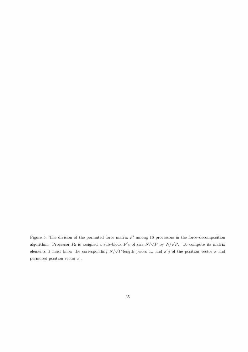
Figure 5: The division of the permuted force matrix F ′ among 16 processors in the force–decomposition

algorithm. Processor P6 is assigned a sub–block F ′6 of size N/

√P by N/

√P . To compute its matrix

elements it must know the corresponding N/√

P -length pieces xα and x′β of the position vector x and

permuted position vector x′.

35

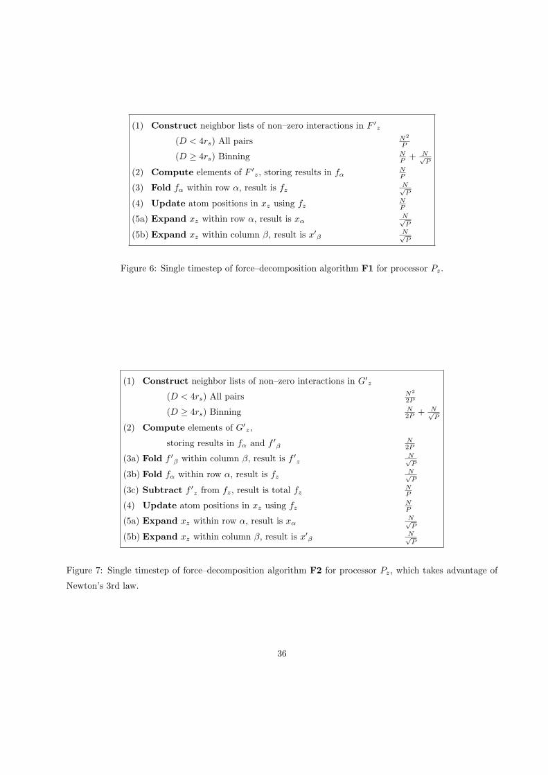
(1) Construct neighbor lists of non–zero interactions in F ′z

(D < 4rs) All pairs N2

P

(D ≥ 4rs) Binning NP + N√

P

(2) Compute elements of F ′z, storing results in fα

NP

(3) Fold fα within row α, result is fzN√P

(4) Update atom positions in xz using fzNP

(5a) Expand xz within row α, result is xαN√P

(5b) Expand xz within column β, result is x′βN√P

Figure 6: Single timestep of force–decomposition algorithm F1 for processor Pz.

(1) Construct neighbor lists of non–zero interactions in G′z

(D < 4rs) All pairs N2

2P

(D ≥ 4rs) Binning N2P + N√

P

(2) Compute elements of G′z,

storing results in fα and f ′βN2P

(3a) Fold f ′β within column β, result is f ′zN√P

(3b) Fold fα within row α, result is fzN√P

(3c) Subtract f ′z from fz, result is total fzNP

(4) Update atom positions in xz using fzNP

(5a) Expand xz within row α, result is xαN√P

(5b) Expand xz within column β, result is x′βN√P

Figure 7: Single timestep of force–decomposition algorithm F2 for processor Pz, which takes advantage of

Newton’s 3rd law.

36

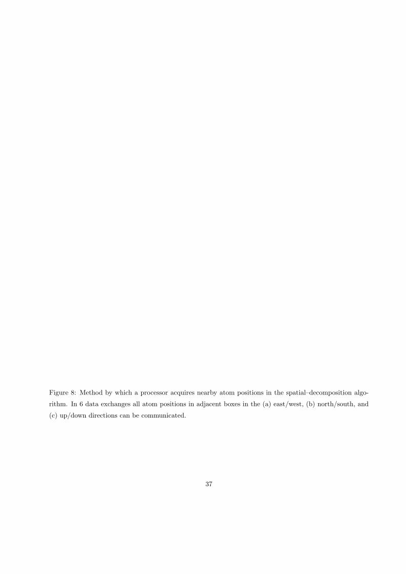
Figure 8: Method by which a processor acquires nearby atom positions in the spatial–decomposition algo-

rithm. In 6 data exchanges all atom positions in adjacent boxes in the (a) east/west, (b) north/south, and

(c) up/down directions can be communicated.

37

(1a) Move necessary atoms to new boxes ∆

(1b) Make lists of all atoms that will need to be exchanged ∆

(1c) Construct neighbor lists of interaction pairs in box z

(d < 2rs) All pairs NP ( N

2P + ∆)

(d ≥ 2rs) Binning N2P + ∆

(2) Compute forces on atoms in box z, doubly storing results in fzN2P + ∆

(4) Update atom positions xz in box z using fzNP

(5) Exchange atom positions across box boundaries

with neighboring processors NP (1 + 2rs/d)3

(d < rs) Send N/P positions to many neighbors rs3

(d ≈ rs) Send N/P positions to nearest neighbors NP

(d > rs) Send positions near box surface to nearest neighbors (NP )

2/3

Figure 9: Single timestep of spatial–decomposition algorithm S1 for processor Pz.

38

Table IV: CPU seconds/timestep for optimized versions of the spatial–decomposition algorithm S1 on the

Intel Paragon for the benchmark simulation. The first two columns are for the Fortran version of the code

run in single– and dual–processor mode. The second two columns are timings with an assembler version of

the force–computation subroutine, again for single– and dual–processor mode.

39

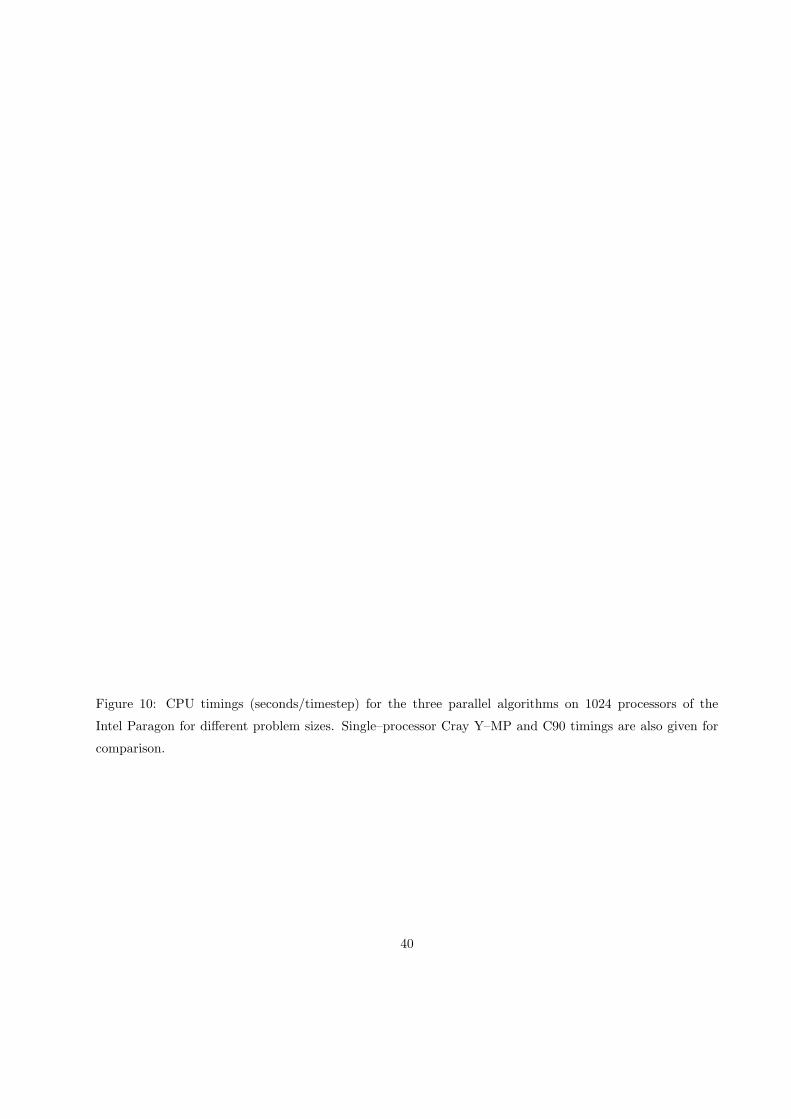
Figure 10: CPU timings (seconds/timestep) for the three parallel algorithms on 1024 processors of the

Intel Paragon for different problem sizes. Single–processor Cray Y–MP and C90 timings are also given for

comparison.

40

Figure 11: CPU timings (seconds/timestep) for the three parallel algorithms on the nCUBE 2 for different

numbers of processors on the benchmark simulation with N = 10976 atoms for two different force cutoff

lengths. Single–processor Cray Y–MP and C90 timings are shown for comparison.

41

Table V: Scaling properties of all 5 parallel algorithms as a function of problem size N and number of

processors P . Run time scaling for the computation and communication portions of the algorithms as well

as their per–processor memory requirements are listed.

42