Fast Online Learning and Detection of Natural Landmarksfor Autonomous Aerial Robots

M. Villamizar, A. Sanfeliu and F. Moreno-NoguerInstitut de Robòtica i Informàtica Industrial, CSIC-UPC

{mvillami,sanfeliu,fmoreno}@iri.upc.edu

Abstract— We present a method for efficiently detectingnatural landmarks that can handle scenes with highly repetitivepatterns and targets progressively changing its appearance.At the core of our approach lies a Random Ferns classifier,that models the posterior probabilities of different views of thetarget using multiple and independent Ferns, each containingfeatures at particular positions of the target. A Shannon entropymeasure is used to pick the most informative locations of thesefeatures. This minimizes the number of Ferns while maximizingits discriminative power, allowing thus, for robust detections atlow computational costs. In addition, after offline initialization,the new incoming detections are used to update the posteriorprobabilities on the fly, and adapt to changing appearances thatcan occur due to the presence of shadows or occluding objects.All these virtues, make the proposed detector appropriate forUAV navigation. Besides the synthetic experiments that willdemonstrate the theoretical benefits of our formulation, wewill show applications for detecting landing areas in regionswith highly repetitive patterns, and specific objects under thepresence of cast shadows or sudden camera motions.

I. INTRODUCTION

Statistical methods for object detection and categorizationhave achieved a degree of maturity that makes them robust toseveral challenging conditions such as target scaling, 2D and3D rotations, nonlinear deformations and lighting changes[6], [8], [10], [14], [21], [19], [26], [28], [30]. Yet, most ofthese approaches involve complex computations, preventingits use in systems requiring online video processing. Thislimitation is specially critical when designing perceptionalgorithms for Unmanned Aerial Vehicle (UAVs), where bothreal time and robustness are mandatory characteristics.

Most current UAV perception algorithms use externalmarkers placed along the environment or on the object ofinterest, which can be easily detected with RGB or infra-red cameras. Tasks such target detection [12], [15], [18],navigation [9], [31] and landing [7], [24] can be easilysimplified with the use of these markers. There are, however,situations where the deployment of markers is not practical orpossible, especially when the vehicle operates in dynamicallychanging and outdoor scenarios.

In this paper, we propose an efficient algorithm fordetecting the pose of natural landmarks on input videosequences without the need of using external markers. Thisis especially remarkable, as we consider scenes like the oneshown in Fig. 1, where the target is a chunk of grass inwhich identifying distinctive interest points is not feasible,preventing thus the use of keypoint recognition methods [13],

Fig. 1. Detecting natural landmarks. Top: Kind of outdoor scenariowe consider. Some of the challenges our detector needs to address arelight changes, shadows and repetitive textures. Bottom: Schematic of theapproach we propose. It consists of two stages, an offline learning stagewhere a general model of the object’s appearance is learned, and an onlinestage, where the object’s model is continuously updated using input images.

[20]. In addition, our approach continuously updates thetarget model upon the arrival of new data, being able to adaptto dynamic situations where the its appearance may change.This is in contrast to the previous approaches, which learnobject appearances from large training datasets, but oncethese models are learned, they are kept unchanged duringthe whole testing process.

As shown in Fig. 1, our approach consists of two mainstages. Initially, a canonical sample of the target is providedby the user as a bounding box in the first frame of thesequence (Fig. 1(a)). Through synthetic warps based on shiftsand planar rotations, new samples of the target are generated,each associated to a specific viewpoint (Fig. 1(b)). All thesesamples are used for training a classifier that models theposterior of each view (Fig. 1(c)). At the core of the classifierthere are Ferns features [22] that given an input trainingsample, model its appearance by combining random setsof binary intensity differences. Yet, in contrast to [22] that

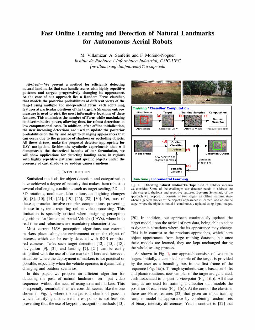
Fig. 2. Failure of keypoint-based methods. Top: Matching of SIFT features (red lines) between the visual target (small top-left image) and a sequenceof image examples that includes lighting and viewpoint changes. Bottom: Output of the proposed detection approach (red circles) for the same target andsequence. Black circles indicate the ground truth and the rectangle shows the detection rates: true positives (TP), false positives (FP) and false negatives (FN).

randomly picks the location of each Fern feature within theimage, we propose a strategy that uses an entropy reductioncriterion for this purpose. This will let us to both minimizethe number of Ferns to represent the target (making thealgorithm more efficient), and maximize the discriminativepower of the classifier. All this initial training is performedoffline, in matter of minutes.

In the second stage (Fig. 1(d)) the classifier is evaluatedat each input frame, and its detections are used to update theposterior probabilities, which still contain the information ofthe original target appearance that avoids drifting to falsedetections (Fig. 1(e)). This allows a non-supervised adaptionof the classifier to progressive target changes.

All these ingredients (markerless, efficient and adapt-able) make our approach appropriate for Autonomous AerialRobots applications. After showing the theoretical benefitsof the method using synthetic data, we will describe severalreal experiments in which our classifier will be used to detectthe position and orientation of natural landmarks in outdoorenvironments where a UAV is expected to operate.

II. RELATED WORK

Marker-based ApproachesThe standard approach for estimating the location of an aerialmobile robot or specific objects of its environment relies onvisual markers introduced in the scene. These markers canbe either perceived by RGB cameras [7], [24] or infraredsensors [9], [17]. Especially the latter, provide very accuratepose estimation results and at a high frame rate, allowingto design accurate control laws and perform complex taskssuch as that of cooperative grasping and manipulation withmultiple aerial vehicles [16].

There are situations, though, in which deploying thesemarkers is not possible or convenient. For instance, theresponse of an infra-red sensor is easily washed out bysunlight in outdoors scenarios. In other circumstances, thetarget to be tracked or detected is chosen on the fly, and isnot possible to place markers on it. In this kind of situations,passive and non-invasive techniques such as those based invision alone, come into play.

Markerless Vision-based ApproachesRemind that our goal is to locate the position and the in-plane orientation of a given target in an input image orvideo sequence. One obvious solution for this is based onalgorithms that first extract points of interest from the inputand target images, represent them with a potentially complexdescriptor [1], [14], and match them using a robust algorithmfor outlier rejection [13], [20], [25]. Yet, in the situationswe consider with natural landmarks, repetitive patterns (likegrass) and lighting artifacts, extracting reliable and salientpoints of interest is not an easy task. Observe, for instance,the example in Fig. 2, where SIFT descriptors are usedto match points of interest of the natural target seen fromdifferent viewpoints. Note that the percentage of matches isvery large for the first images but it decreases significantlyfor the next ones because of lighting and viewpoint changes.Therefore, these point based algorithms have been mostlyused in indoor applications with controlled light conditions.Indeed, we can find some recent works that under these con-straints have been shown effective for UAV navigation [4],visual tracking [18] and target detection [27].

When single feature points are not reliable cues, onecan model the appearance of the whole target object. Thiscan be expressed as a classification problem, where eachtarget orientation corresponds to a different class. There arepotentially many algorithms which could be used for thistask, and which have been shown to give excellent results inobject detection applications [6], [8], [23], [26]. Yet, mostof them have a high computational cost and require rigoroustraining procedures for being effectively implemented inaerial robots.

The approach we present here falls within this group ofmethods, but we alleviate the computational cost of our clas-sifier using two strategies. First, we split the learning processin two stages, one offline and the other online. This helpsto reduce the amount of information included in the modeland thus, reduces its complexity. And second, we proposean optimization strategy based on entropy minimization, inwhich the number of features is minimized while retainingtheir discriminative power. The essence of this strategy is

Fig. 3. Synthetic training data. The canonical sample (left) is synthetically warped to generate new training samples (middle). These samples arecomputed at different orientations and at different shift and blurring levels (right). The red circle and arrow indicate the target pose for each sample.

sample sample

Fig. 4. Fern-based classifier. Computation of the classifier using J = 2 Ferns with M = 2 binary features. Left: Schematic representation of the Fernsstructure using binary trees. At the bottom of the tree we plot the distributions which are updated for a training sample x. For instance, assuming the trainingsample x belongs to the positive class and that F1(x) = (00)2 + 1 = 1, the bin of the positive class in z = 1 would be increased in one unit. The samesample, would also increase in one unit the bin corresponding to z = 3 of F2, as F2(x) = (10)2 + 1 = 3. Right: Example of how the Ferns are testedon an image sample x. Features are signed comparisons between image pixels. (u, v) denote the spatial coordinate, and c the color channel coordinate.

similar to what is done in recent works with two-classclassification problems [11], [29], [30]. Yet, these works arenot applicable to our multiview-classification problem.

III. APPROACH

We next describe the main steps for building the classifier:generation of an initial set of synthetic samples, offlineconstruction of the classifier, a new criteria for selecting thefeatures, and finally, the online adaption of the algorithm.

A. Generating Synthetic Samples for Offline Training

We initially assume that we only have one single sampleof the target we seek to detect. This canonical sample isprovided by the user as a bounding box in the first frameof the video sequence. In order to obtain a more completedescription of the target we synthetically generate new viewsof the canonical shape.

As it is typically done in aerial imagery, the depth of thetarget is assumed negligible compared to its distance w.r.t. thecamera. We therefore consider the canonical target as beingplanar, and approximate the multiple views it can take as in-plane rotations. Note, however, that our approach is equallyvalid for non-planar objects. In that case, sample trainingimages could be either generated with more sophisticatedrendering tools or by simply acquiring real images of thetarget from each of the viewpoints.

For the purposes of this paper, and as shown in theexample of Fig. 3, the canonical shape is rotated at W = 12principal pose orientations, that will establish the classesof our classification problem. In addition, for each posew ∈ {1, 2, ..,W} we further include 6 additional samples

with random levels of shifting and blurring. This helps tomodel small deviations from the planar assumption, as wellas the blurring produced by sudden motions of the camera.A final subset with a similar number of background samples(random patches chosen from background) per pose is alsoconsidered. We denote this whole initial training dataset asD = {(xi, yi)}Ni=1 where xi ∈ X corresponds to a samplein the image space X , N is the number of samples, andyi = {+wi,−wi} is the class label, indicating if the samplebelongs to the pose w or background classes, respectively.

B. Building the Classifier

In order to perform online learning and object detection,we use Random Ferns (RFs) [22]. This classifier can beunderstood as an extreme and very fast implementation of arandom forest [5] which combines multiple random decisiontrees. Furthermore, subsequent works have shown the RFs tobe robust to over-fitting and that they can be progressivelycomputed upon the arrival of new data [11], [29]. The mostdistinctive characteristic of RFs compared to the classicalrandom forests is that the same test parameters are used inall nodes of the tree level [5], [22]. We show this in Fig. 4-left, where we can see two Ferns F , each one with twodecision tests or binary features f .

More formally, the online classifier is built as an averageof J Ferns in which each Fern Fj consists of a set of Mbinary features, Fj = {f j1 , f

j2 , . . . , f

jM}, representing binary

comparisons between pairs of pixel intensities. This can bewritten as

f(x) = I(x(u1, v1, c1) > x(u2, v2, c2))

where x is the image sample, x(u, v, c) indicates the imagevalue at pixel coordinates (u, v) with color channel c, andI(e) is the indicator function:

I(e) ={

1 if e is true0 if e is false

As we will describe in the following subsection, and incontrast to the original Ferns formulation [22], the locationof these pairs of pixels is computed during the training stageaccording to a criterion of entropy minimization. Fig. 4-right shows a simple example of how two different Fernswith two features are evaluated in an image sample x. Thecombination of these binary features determines the Fernoutput, F (x) = z, where z = (f1, . . . , fM )2 + 1, is theco-occurrence of the features and corresponds to the Fernleaf where the sample x falls (See Fig. 4-left).

So far, we have discussed how a single Fern is evaluatedon an image sample. Let us now explain how the classifieris built, from the response of J Ferns F = {F1, . . . , FJ}.The response of the classifier, for an input sample image xcan be written as

H(x) =

{+1 if conf(x ∈ w) > β−1 otherwise,

where w is the estimated pose of the sample, conf(x ∈ w) isthe confidence of the classifier on predicting that x belongsto the class w, and β is a confidence threshold whose defaultvalue is 0.5. Thus, if the output of the classifier for asample x is H(x) = +1, the sample is assigned to the target(positive) class w. Otherwise, it is assigned to the background(negative) class. The confidence of the classifier is definedaccording to the following posterior:

conf(x ∈ w) = p(y = +w|F(x),θ), (1)

where θ are parameters of the classifier we will define belowand y = {+w,−w} denotes the class label.

The estimated pose w is computed by evaluating theconfidence function over all possible poses, and picking theone with maximum response, i.e.:

w = argmaxw

p(y = +w|F(x),θ), w = 1, . . . ,W

As said before, this posterior probability is computed bycombining the posterior of the J Ferns:

p(y = +w|F(x),θ) = 1

J

J∑j=1

p(y = +w|Fj(x) = z, θj,z,w),

where z is the Fern output, and θj,z,w is the probability thata sample in the Fern j with output z belongs to the positiveclass with pose w. Since the posterior probabilities follow aBernoulli distribution

p (y|Fj(x) = z, θj,z,w) ∼ Ber(y|θj,z,w),with we can write that

p (y = +w|Fj(x) = z, θj,z,w) = θj,z,w

The parameters of these distributions are computed duringthe training stage through a Maximum Likelihood Estimate

Fig. 5. Feature selection process. Example of the kind of distributionswe consider in the Fern leaves, for a case where we have two classes orposes w. Each distribution H encodes the amount of positive and negativesamples, for each of the classes.

(MLE) over the labeled set of synthetic samples D we havepreviously generated. That is,

θj,z,w =N+w

j,z

N+wj,z +N−wj,z

(2)

where N+wj,z is the number of positive samples that fall into

the leaf z of the Fern j. Similarly, N−wj,z corresponds to thenumber of negative samples for the Fern j with output z. Thereader is referred to Fig. 4-left for an illustrative example.

C. Feature Selection

In all previous works that use RFs classifiers, the Fernsfeatures, i.e, the pairs of pixels whose intensities are com-pared, are chosen at random [11], [22], [29]. In this paper weclaim, and we will demonstrate it in the results, that a moreprincipled approach for selecting those features can lead toincreased levels of efficiency and robustness.

For this purpose we propose a methodology to choose thebinary features that reduce the classification error over thetraining data D. As an approach to this, we will seek for thefeatures that minimize the Shannon Entropy E , which givesa measure about the impurity of the tree (i.e, how peakedare the posterior distributions at each Fern), and about theuncertainty associated with the data [3], [26].

More specifically, each Fern Fj is independently computedfrom the rest of Ferns, and using a different and smallrandom subset S ⊆ D of the training data. Partitioning thetraining data will avoid potential overfitting errors duringtesting [3], [5]. Let us now assume we have a large andrandom pool of binary features, and we want to pick thebest of them for a Fern Fj . At each node level m, we willchoose the binary feature fm that minimizes the entropy ofthe Fern E(Fj), computed as

E(Fj) =

2m∑z=1

−Nj,z

|S|E(Hz), E(Hz) = −Hz logHz,

where Nj,z is the number of samples falling into the leaf zand |S| is the size of the samples subset S. The variable Hz

is the distribution of samples across poses w in the leaf z, andis represented trough a normalized histogram (See Fig. 5).

Once the feature fm that minimizes E(Fj) is chosen, itis added to the set of features of Fj . This is repeated untila maximum number of features M (corresponding the thedepth of the Fern) is reached. The pseudocode of the wholeprocedure for building the classifier is presented in Alg. 1.

0 0.1 0.2 0.3 0.4 0.5 0.6 0.7 0.8 0.9 10

0.1

0.2

0.3

0.4

0.5

0.6

0.7

0.8

0.9

1

Random Selection − EER: 60.00%

0.5

0.55

0.6

0.65

0.7

0.75

0 0.1 0.2 0.3 0.4 0.5 0.6 0.7 0.8 0.9 10

0.1

0.2

0.3

0.4

0.5

0.6

0.7

0.8

0.9

1

conf(x)

Positive/TargetNegative/Background

0 0.1 0.2 0.3 0.4 0.5 0.6 0.7 0.8 0.9 10

0.1

0.2

0.3

0.4

0.5

0.6

0.7

0.8

0.9

1

Proposed Approach − EER: 87.89%

0.5

0.55

0.6

0.65

0.7

0.75

0.8

0.85

0.9

0.95

0 0.1 0.2 0.3 0.4 0.5 0.6 0.7 0.8 0.9 10

0.1

0.2

0.3

0.4

0.5

0.6

0.7

0.8

0.9

1

conf(x)

Positive/TargetNegative/Background

Fig. 6. Random Ferns (Top) vs Entropy-based Ferns (Bottom). Left: The proposed approach is compared to standard RFs in a two-class syntheticproblem. Cyan and red symbols correspond the the two main classes, positive and negative respectively, and the + and 0 are two additional values thateach element of every class can take. Black symbols indicate misclassified samples. Middle: Maps showing the response of the classifiers on the densesample space. Right: Distributions of positive and negative classes according to the confidence conf(x) of the classifiers, computed from Eq. 1.

In order to highlight the advantages of the Entropy-basedapproach for selecting features, compared to the standardrandom approach, we have performed the toy experimentsummarized in Fig. 6. The problem consists in building aclassifier for a two-class (red and cyan classes) problem,where each class element may take two possible values(“+” and “0”). The binary features in this example areaxis-aligned split functions (2D decision stumps) with arandom threshold. That is, given a sample x with coordinates(u, v) ∈ [0, 1]× [0, 1] we compute binary features as

f(x) = (p > λ) ,

where p = {u, v} corresponds to one of the axis, and λ arandom threshold in the interval [0, 1]. We train the classifierswith 20 Ferns and 7 such features per Fern.

The left-most column of Fig. 6 shows the response ofboth classifiers to new testing data, where black “0” or“+” symbols are misclassified samples. As expected, theclassification results are consistently better when using theEntropy for selecting the features. This is also illustratedin the dense classification maps shown in Fig. 6-middle,where the response of the our classifier, clearly yields a moreprecise information about the spatial layout of each of theclasses.

Another advantage of the proposed classifier is that itprovides a greater separation between positive and negativeclasses than standard RFs, being thus more discriminative.This is shown in the right-most column of Fig. 6, where weplot the confidence value of Eq. 1 for each of the classes.

D. Online Learning

The offline training procedure described in the previoussection can be done in about one minute (for M ≈ 3 featuresand J ≈ 20 trees). Then, at runtime, the resulting classifier isevaluated over the input data and it is continuously updatedin order to adapt to potential changes undergone by the targetobject.

As shown in the approach overview in Fig. 1, duringthe online learning process, new detections are fed into the

Algorithm 1: Feature Selection & Building the ClassifierInput:-J : Number of Ferns.-M : Number of binary features.-D = {(xi, yi)}Ni=1: Training dataset consisting of Nimage samples x ∈ X , where yi ∈ {+w,−w} is thelabel for the target and background classes with posew, respectively.Output: Visual target classifier H(x).

1 for j = 1; j ≤ J do2 Sample at random a reduced set of images S ⊆ D

from the training data D.3 for m = 1;m ≤M do4 Compute a set of K random binary features.5 for k = 1; k ≤ K do6 Test feature fk on the sample set S.7 Compute the entropy of the current Fern j,

E(Fj) =∑2m

z=1−Nj,z

|S| E(Hz)

8 Select the feature fm that minimizes E(Fj).9 Add feature fm to the Fern fm → Fj .

10 Assemble the computed Ferns Fj → F.

classifier to update the posterior probabilities. These samplesare labeled as either positive, corresponding to the target, ornegative, when they correspond to the background.

The labeling is done based on the confidence value aboutthe input sample x computed using Eq. 1. If a sample x withpose w has a confidence value conf(x) > β, it is assigned tothe positive class +w. Otherwise, the sample is considerednegative −w. The parameter β is the threshold of theclassifier and to reduce the risk of misclassification it is set tothe Bayes error rate. Yet, since an incorrect labeling mightlead to drifting problems and loss of the target, we makeuse of a more rigorous rejection criterion [2], and we set aconfidence interval γ around β to indicate predictions with

ERFs RFs ERFs RFs

0.55 0.57 0.45 0.55

0.66 0.67 0.62 0.65

0.72 0.79 0.82 0.85

0.77 0.86 0.86 0.87

# Ferns

# F

eatu

res

5 10 20 50

3

5

7

9

0.46 0.46 0.48 0.44

0.60 0.52 0.44 0.51

0.52 0.57 0.63 0.63

0.63 0.65 0.61 0.64

# Ferns

# F

eatu

res

5 10 20 50

3

5

7

9

0.96 0.97 0.99 0.97

0.92 0.90 0.93 0.89

0.83 0.67 0.61 0.57

0.74 0.53 0.47 0.49

# Ferns

# F

eatu

res

5 10 20 50

3

5

7

9

0.99 0.98 0.97 0.98

0.98 0.96 0.99 0.99

0.97 0.96 0.92 0.93

0.93 0.89 0.94 0.90

# Ferns

# F

eatu

res

5 10 20 50

3

5

7

9

Fig. 7. 2D classification problem. Evaluation of ERFs (first and third columns) against RFs (second and fourth columns). Left: Classification performanceof both classifiers measured trough precision-recall rates. Right: Degree of overlapping between positive and negative class distributions.

ambiguous confidence values. Samples within this intervalare not further considered in the updating process.

The labeled samples that pass the confidence test are thenused to recompute the prior probabilities θj,z,w of Eq. 2, andupdate the classifier. For instance, let us assume that a samplex is labeled as +wi, and that it activates the output z of thefern Fj , i.e, Fj(x) = z. We will then update the classifier byadding one unit to the i-th bin of the histogram of N+w

j,z . Thisis repeated for all ferns. With these new distributions, we canrecompute the priors θj,z,w, and thus, update the classifier.

IV. EXPERIMENTS

We next evaluate the proposed method, dubbed ERFs (forEntropy-based Random Ferns), using both synthetic data andreal experiments of detection of natural landmarks.

A. 2D Classification Problem

This experiment has already been presented in the previoussection to evaluate different characteristics of the ERFs andcompare them against a classifier whose Ferns are computedcompletely at random (RFs). In Fig. 6 we have alreadyshown some qualitative results that visually demonstrate theadvantages of our approach. We next present a more in-depthanalysis of two approaches.

We first analyze the amounts of Ferns and features used tocompute both types of classifiers. Fig. 7-(two leftmost plots)represents the classification performance of these approachesthrough the Equal Error Rate (EER) over precision and recallscores. Note that the classification rates grow with the sizeof the classifier, and that ERFs consistently obtain higherclassification rates than RFs, even when for smaller amountsof features and Ferns.

Another advantage of the proposed classifier is that ityields larger degrees of separability between the positive andnegative classes. We already qualitatively observed this inFig. 6. In the new Fig. 7-(two rightmost plots) we numer-ically demonstrate this using the Bhattacharyya coefficient,that measures the amount of overlap between distributions.We clearly see that ERFs provide lower coefficients than theclassifier computed at random (RFs). This is critical for on-line learning and detection, as it reduces the misclassificationerror and possible drifting problems.

RFs ERFs0.55

0.6

0.65

0.7

0.75

0.8

0.85

0.9

0.95

1

ApproachesP

R−

EE

R

5 Ferns10 Ferns20 Ferns50 Ferns

28.23 24.47 21.53 18.63

19.32 16.50 13.75 11.51

12.29 9.61 7.91 6.41

5.80 4.33 3.39 2.72

# Ferns

# F

eatu

res

5 10 20 50

3

5

7

9

Fig. 8. Detection of ground patches. Left: Detection rates according tothe number of Ferns used to compute the classifier. Right: Speed of theclassifier (frames per second) for different amounts of features and Ferns.

B. Detection of Ground Patches

We next use the ERFs classifier to detect specific patcheson the ground, in a field containing a mixture of grassand soil. While this is a very useful task for detectinglanding areas for UAVs it is extremely challenging, due tothe presence of many similar patterns, and the lack of salientand recognizable visual marks. Fig. 12-(top, middle) showsa few sample images.

Like in the previous experiment, we again compare theERFs and RFs. To this end, we evaluate the classifiers ina video sequence containing 150 images of a ground field,that suffers from several artifacts, such as sudden cameramotions, and light and scale changes (see Fig. 12-top). In thisexperiment, we considered 9 features per Fern. The detectionperformance rate of both methods are presented in Fig. 8-left, where we detail the PR-EER (Equal Error Rate overthe Precision-Recall curve) values for classifiers trained withdifferent numbers Ferns. Note again that the ERFs classifieryields better results and is less sensitive to the number ofFerns, thus allowing for more efficient evaluations. This isverified in Fig. 8-right where we provide the computationtime of the classifiers in frames per second. Some sampleimages with the outputs of the ERFs (red circles) and theRFs (green ones) are depicted in Fig. 12-top. Observe thatthe ERFs are able to accurately detect the visual target, evenwhen it is difficult for the human eye.

Fig. 12-middle shows another experiment of recognizingground landmarks. This experiment contains 64 imageswhere the target appears at multiple locations and under

RFs ERFs0

0.2

0.4

0.6

0.8

1

Approaches

PR

−E

ER

5 Ferns10 Ferns20 Ferns50 Ferns

RFs ERFs0

0.1

0.2

0.3

0.4

0.5

Overlappin

g

Approaches

5 Ferns 10 Ferns20 Ferns50 Ferns

Fig. 9. Landmark detection performance. ERFs are evaluated andcompared to RFs using different number of Ferns (left), and according tothe degree of overlapping between the target and background classes (right).

NCC RFs ERFs (Off) ERFs0

0.2

0.4

0.6

0.8

1

Approaches

PR

−E

ER

0 20 40 60 80 100 1200

0.2

0.4

0.6

0.8

1

# Frames

conf(

x)

NCCRFsERF(Off.) ERFs

Fig. 10. Detection of 3D objects. ERFs are assessed to learn and detect3D objects. Left: Detection rates. Right: Output of the classifier conf(x).

various rotations. In this experiment, the classifiers aretrained with W = 16 in-plane possible orientations. Thedetection rates of both the ERFs and the RFs are shownin Fig. 9-left. Again, the ERFs provide better results. Inaddition, if we analyze the degree of overlapping betweenthe target and background classes through the Bhattacharyyacoefficient (Fig. 9-right), we see that ERFs provide muchhigher separation of classes, and therefore, much higherconfidence values in its detection. Observe in Fig. 12-middlea few sample results where both the position and orientationof the target are correctly estimated. Indeed, the proposedmethod yields a detection rate over 95% (PR-EER) and anorientation accuracy of 93%.

C. 3D Object Detection

We have also tested our approach in objects that do notsatisfy the assumption we made of having a depth which isnegligible compared to its distance to the camera. Fig. 12-bottom shows a few samples of a 120 frames sequence of abench seen from different viewpoints and scales.

In this case we have included in the analysis a templatematching approach based on Normalized Cross Correlation(NCC), widely used for detecting specific objects. The recog-nition results of all methods are summarized in Fig. 10-left.Observe that the performance of NCC is quite poor. Thisis because a plain NCC template matching can not adaptthe appearance changes produced different viewpoints. Thesame limitation would suffer our approach without the onlineadaption, shown in the figure as ERFs (Off). This behavioris also reflected in Fig. 10-right that plots the confidenceconf(x) of each classifier along the sequence. ERFs (Off.)

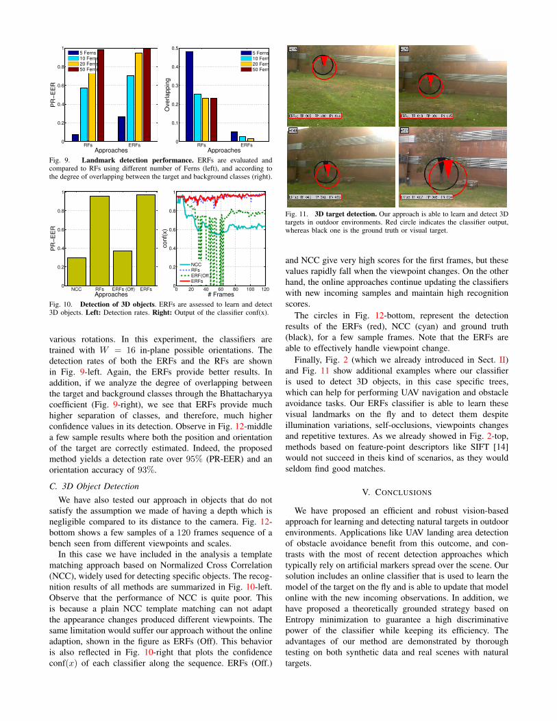
Fig. 11. 3D target detection. Our approach is able to learn and detect 3Dtargets in outdoor environments. Red circle indicates the classifier output,whereas black one is the ground truth or visual target.

and NCC give very high scores for the first frames, but thesevalues rapidly fall when the viewpoint changes. On the otherhand, the online approaches continue updating the classifierswith new incoming samples and maintain high recognitionscores.

The circles in Fig. 12-bottom, represent the detectionresults of the ERFs (red), NCC (cyan) and ground truth(black), for a few sample frames. Note that the ERFs areable to effectively handle viewpoint change.

Finally, Fig. 2 (which we already introduced in Sect. II)and Fig. 11 show additional examples where our classifieris used to detect 3D objects, in this case specific trees,which can help for performing UAV navigation and obstacleavoidance tasks. Our ERFs classifier is able to learn thesevisual landmarks on the fly and to detect them despiteillumination variations, self-occlusions, viewpoints changesand repetitive textures. As we already showed in Fig. 2-top,methods based on feature-point descriptors like SIFT [14]would not succeed in theis kind of scenarios, as they wouldseldom find good matches.

V. CONCLUSIONS

We have proposed an efficient and robust vision-basedapproach for learning and detecting natural targets in outdoorenvironments. Applications like UAV landing area detectionof obstacle avoidance benefit from this outcome, and con-trasts with the most of recent detection approaches whichtypically rely on artificial markers spread over the scene. Oursolution includes an online classifier that is used to learn themodel of the target on the fly and is able to update that modelonline with the new incoming observations. In addition, wehave proposed a theoretically grounded strategy based onEntropy minimization to guarantee a high discriminativepower of the classifier while keeping its efficiency. Theadvantages of our method are demonstrated by thoroughtesting on both synthetic data and real scenes with naturaltargets.

Fig. 12. Visual target detection. Output of the proposed approach (red circles) for detecting ground targets (top, middle) and 3D objects (bottom). Blackcircles denote the location of the targets, whereas the rectangle shows the detection rates: true positives (TP), false positives (FP) and false negatives (FN).

VI. ACKNOWLEDGMENTS

This work was partially supported by the projects PAU+DPI2011-27510, RobTaskCoop DPI2010-17112, ERA-NetChistera project ViSen PCIN-2013-047, and by the EUproject ARCAS FP7-ICT-2011-28761.

REFERENCES

[1] H. Bay, T. Tuytelaars, and L. Van Gool. SURF: Speeded up robustfeatures. In ECCV, 2006.

[2] C. M. Bishop. Pattern recognition and machine learning. Springer,2006.

[3] Leo Breiman. Random forests. Machine Learning, 45(1):5–32, 2001.[4] A. Cesetti, E. Frontoni, A. Mancini, P. Zingaretti, and S. Longhi.

A vision-based guidance system for uav navitagion and safe landingusing natural landmarks. Journal of intelligent and robotic systems,57(1):233–258, 2010.

[5] A. Criminisi, J. Shotton, and E. Konukoglu. Decision forests: A unifiedframework for classification, regression, density estimation, manifoldlearning and semi-supervised learning. Foundations and Trends inComputer Graphics and Vision, 7(2–3):81–227, 2011.

[6] N. Dalal and B. Triggs. Histograms of oriented gradients for humandetection. In CVPR, 2005.

[7] Y. Fan, S. Haiqing, and W. Hong. A vision-based algorithm for landingunmanned aerial vehicles. In International Conference on ComputerScience and Software Engineering, pages 993–996, 2008.

[8] P.F. Felzenszwalb, R.B. Girshick, D. McAllester, and D. Ramanan.Object detection with discriminatively trained part-based models.PAMI, 32(9):1627–1645, 2010.

[9] G. Flores, S. Zhou, R. Lozano, and P. Castillo. A vision and gps-basedreal-time trajectory planning for mav in unknown urban environments.In ICUAS, 2013.

[10] S. Hinterstoisser, V. Lepetit, P. Fua, and N. Navab. Dominantorientation templates for real-time detection of texture-less objects.In CVPR, 2010.

[11] Z. Kalal, J. Matas, and K. Mikolajczyk. P-N learning: Bootstrappingbinary classifiers by structural constraints. In CVPR, 2010.

[12] J. Kim and D.H. Shim. A vision-based target tracking control systemof a quadrotor by using a tablet computer. In ICUAS, 2013.

[13] V. Lepetit and P. Fua. Keypoint recognition using randomized trees.PAMI, 28(9):1465–1479, 2006.

[14] D.G. Lowe. Distinctive image features from scale-invariant keypoints.IJCV, 60(2):91–110, 2004.

[15] A. Masselli, S. Yang, K.E. Wenzel, and A. Zell. A cross-platformcomparison of visual marker based approaches for autonomous flightof quadrocopters. In ICUAS, 2013.

[16] D. Mellinger, M. Shomin, N. Michael, and V. Kumar. Cooperativegrasping and transport using multiple quadrotors. Distributed au-tonomous robotic systems, pages 545–558, 2013.

[17] N. Michael, D. Mellinger, Q. Lindsey, and V. Kumar. The graspmultiple micro-uav testbed. Robotics and Automation Magazine,17(3):56–65, 2013.

[18] I.F. Mondragon, P. Campoy, J.F. Correa, and L. Mejias. Visual modelfeature tracking for uav control. In IEEE International Symposium onIntelligent Signal Processing, pages 1–6, 2007.

[19] F Moreno-Noguer, J Andrade-Cetto, and A Sanfeliu. Fusion of colorand shape for object tracking under varying illumination. In PatternRecognition and Image Analysis, pages 580–588, 2003.

[20] F. Moreno-Noguer, V. Lepetit, and P. Fua. Pose priors for simultane-ously solving alignment and correspondence. In ECCV, 2008.

[21] F. Moreno-Noguer, A. Sanfeliu, and D. Samaras. Integration ofdeformable contours and a multiple hypotheses fisher color model forrobust tracking in varying illuminant environments. Image and VisionComputing, 25(3):285–296, 2007.

[22] M. Ozuysal, M. Calonder, V. Lepetit, and P. Fua. Fast keypointrecognition using random ferns. PAMI, 32(3):448–461, 2010.

[23] M. Ozuysal, V. Lepetit, and P. Fua. Pose estimation for categoryspecific multiview object localization. In CVPR, 2009.

[24] J.L. Sanchez-Lopez, S. Saripalli, P. Campoy, J. Pestana, and C. Fu.Toward visual autonomous ship board landing of a vtol uav. In ICUAS,2013.

[25] E. Serradell, M. Ozuysal, V. Lepetit, P. Fua, and F. Moreno-Noguer.Combining geometric and appearance priors for robust homographyestimation. In ECCV, 2010.

[26] J. Shotton, M. Johnson, and R. Cipolla. Semantic texton forests forimage categorization and segmentation. In CVPR, 2008.

[27] A. Symington, S. Waharte, S. Julier, and N. Trigoni. Probabilistictarget detection by camera-equipped uavs. In ICRA, 2010.

[28] M. Villamizar, J. Andrade-Cetto, A. Sanfeliu, and F. Moreno-Noguer.Bootstrapping boosted random ferns for discriminative and efficientobject classification. Pattern Recognition, 45(9):3141–3153, 2012.

[29] M. Villamizar, A. Garrell, A. Sanfeliu, and F. Moreno-Noguer. Onlinehuman-assisted learning using random ferns. In ICPR, 2012.

[30] M. Villamizar, F. Moreno-Noguer, J. Andrade-Cetto, and A. Sanfeliu.Efficient rotation invariant object detection using boosted randomferns. In CVPR, 2010.

[31] S. Yang, S.A. Scherer, and A. Zell. An onboard monocular visionsystem for autonomous takeoff, hovering and landing of a micro aerialvehicle. Journal of intelligent and robotic systems, 69(1–4):499–515,2013.