Fast multipole method for the biharmonic equation in three dimensions

Journal of Computational Physics 215 (2006) 363–383

www.elsevier.com/locate/jcp

Fast multipole method for the biharmonic equation inthree dimensions

Nail A. Gumerov *, Ramani Duraiswami

Perceptual Interfaces and Reality Laboratory, Department of Computer Science and UMIACS, Institute for Advanced

Computer Studies, University of Maryland, Room 3305 A.V. Williams Building, College Park, MD 20742, United States

Received 17 May 2005; received in revised form 5 October 2005; accepted 31 October 2005Available online 13 December 2005

Abstract

The evaluation of sums (matrix–vector products) of the solutions of the three-dimensional biharmonic equation can beaccelerated using the fast multipole method, while memory requirements can also be significantly reduced. We develop acomplete translation theory for these equations. It is shown that translations of elementary solutions of the biharmonicequation can be achieved by considering the translation of a pair of elementary solutions of the Laplace equations. Theextension of the theory to the case of polyharmonic equations in R3 is also discussed. An efficient way of performingthe FMM for biharmonic equations using the solution of a complex valued FMM for the Laplace equation is presented.Compared to previous methods presented for the biharmonic equation our method appears more efficient. The theory isimplemented and numerical tests presented that demonstrate the performance of the method for varying problem sizes andaccuracy requirements. In our implementation, the FMM for the biharmonic equation is faster than direct matrix–vectorproduct for a matrix size of 550 for a relative L2 accuracy �2 = 10�4, and N = 3550 for �2 = 10�12.� 2005 Elsevier Inc. All rights reserved.

1. Introduction

Many problems in fluid mechanics, elasticity, and in function fitting via radial-basis functions, at their core,require repeated evaluation of the sum

0021-9

doi:10.

* CoE-m

wðqjÞ ¼XN

i¼1

Uðqj; riÞqi; j ¼ 1; . . . ;M ; ð1Þ

where Uðqj; riÞ : R3 ! R is a solution of the three-dimensional biharmonic equation (e.g. the Green�s functionor a multipole solution) centered at ri. This sum must be evaluated at locations qj, and qi are some coefficients.Straightforward computation of these sums, which also can be considered to be multiplication of a M · N ma-trix with elements Uji = U(qj, ri) by a N vector with components qi to obtain a M vector with components

991/$ - see front matter � 2005 Elsevier Inc. All rights reserved.

1016/j.jcp.2005.10.029

rresponding author. Tel.: +1 301 405 8210.ail address: [email protected] (N.A. Gumerov).

mailto:[email protected]

364 N.A. Gumerov, R. Duraiswami / Journal of Computational Physics 215 (2006) 363–383

wj = w(qj), obviously requires O(MN) operations and O(MN) memory locations to store the matrix. The pointsets qj (the target set) and ri (the source set) in these problems may be different, or the same. If the points qj andri coincide, the evaluation of U may have to be appropriately regularized in case U is singular (e.g. in a bound-ary element application, quadrature over the element will regularize the function). In the sequel we assumethat this issue, if it arises, is dealt with, and not concern ourselves with it.

In its original form, the fast multipole method, introduced by Greengard and Rokhlin [1], is an algorithmfor speeding up such sums, for the case that the function U is a multipole of the Laplace equation. FMMinspired algorithms have since appeared for the solution of various problems of both matrices associated withthe Laplace potential, and with those of other equations (the biharmonic, Helmholtz, Maxwell) and in unre-lated areas (for general radial-basis functions).

Previous work related to the FMM for the biharmonic equations has usually appeared in the context ofStokes flow or linear elastostatics. The Stokes equations for low Reynolds number fluid flow, and the Lameequations of elastostatics can both be written in the form

r2u ¼ rq; r � u ¼ aq; ð2Þ
where u is the velocity vector for Stokes flow and the displacement vector for elastostatics, the scalar q is pro-portional to the isotropic component of the stress, and a is zero for Stokes flow, and can be expressed via thePoisson ratio for the Lame equations [2]. It is not difficult to show that for a 6¼ 1,
r4u ¼ 0; ð3Þ
i.e., each Cartesian component of the velocity (displacement) satisfies the biharmonic equation.
1.1. Comparison with other FMMs for the biharmonic and related equations

A description of previous applications of the FMM to these problems may be found in the comprehensivereview paper of Nishimura [3]. One approach to the FMM for sums of the biharmonic Green�s function andits derivatives, avoids the problem of building a translation theory for this equation. These Green�s functionsare represented as sums of Laplace solutions [4]. Another approach is based on expanding the biharmonicfunctions in Taylor series [5,6]. Other related FMMs are those that treat the problem of Stokes flow or linearelastostatics, but not directly applicable to the biharmonic translation, have also appeared. These may nothave the efficiency of an FMM derived from a consideration of the elementary solutions of the biharmonicequation. Also we can mention the work of [7], where a kernel independent FMM was developed and appliedto solution of Stokes and other equations.

Perhaps the first to apply the FMM to problems related to the three-dimensional biharmonic equationwas the paper by Sangani and Mo [8], who considered Stokes flow around particles. The method reliedon expansions suggested by Lamb [9], and translation formulae, that are O(p4) when there are O(p2) termsin the Lamb expansion. Greenbaum et al. [10] presented a version of the FMM for the 2D biharmonicequation that use two complex analytic expressions that get translated together. It is thus difficult to extendto R3. It was applied to the solution of some problems in 2D elasticity/Stokes flow in Greengard et al. [11].Popov and Power [6] used Taylor series representations to develop a multipole translation theory for linearelasticity problems. Their results show a cross-over (when the FMM algorithm is faster than the directapproach) for 1.1 · 104 unknowns, though the error that is incurred is hard to establish, as they used aniteration error criterion, which does not have a corresponding value here. They mention that the largestorder of Taylor series considered is 5 in their paper. Fu et al. [4], made the observation that the biharmonicGreen�s function, and its other derivatives could, via elementary manipulations, be written as sums ofLaplace multipoles multiplied by source or target dependent coefficients. For example the biharmonicGreen�s function, can be written as

jr� qj ¼ffiffiffiffiffiffiffiffiffiffiffiffiffiffiffiffiffiffiffiffiffiffiffiffiffiffiffiffiffiffiffiffiffiffiffiffiffiffiffiffiffiffiffiffiffiffiffiffiffiffiffiffiffiffiffiffiffiffiffiffiffiffiffiffiffiffiffiffiffiffiffiðr1 � q1Þ

2 þ ðr2 � q2Þ2 þ ðr3 � q3Þ

2q

¼ jrj2 þ jqj2

jr� qj � 2r1

1

jr� qj q1 � 2r2

1

jr� qj q2 � 2r3

1

jr� qj q3.

N.A. Gumerov, R. Duraiswami / Journal of Computational Physics 215 (2006) 363–383 365

This allowed them to use an existing Laplace multipole method software and achieve an FMM for the elas-tostatics problem. This approach requires more Laplace solutions to represent higher order derivatives. Theuse of this technique for the solution of Stokes problems was presented in [12]. In these papers no explicit‘‘break-even’’ data was presented.

Yoshida et al. [14] improved on the economy with which elasticity problem solutions were represented viaLaplace solutions. They built a solution of the problem based on the Neuber–Papkovich representation of thedisplacement field, which can be expressed in terms of four harmonic functions. The formulation includesfunctions of the type /(r) and r/(r), where / is harmonic. The translation method presented in this case byYoshida [13,14] shows that the complexity of solution of the elastostatic problem using the FMM in thesepapers is equivalent to solution of four independent 3D Laplace equations. Fast translation methods forthe Laplace equation presented in [15,16] where also employed by these authors.

Another field that has seen the use of the FMM for sums of biharmonic and polyharmonic Green�s func-tions is radial-basis interpolation. The biharmonic function is an optimal radial-basis function in a certainsense [17], and scattered data interpolation using these in R3 has been pursued by many authors. Chen andSuter [5] used a Taylor series based FMM to speed the evaluation of spline interpolated 3D data. From theirresults a cross-over point of 13,000 for p = 3 and of 18,000 for p = 4 can be inferred. Carr et al. [18] report onthe application of the FMM to a problem of interpolation with biharmonic splines. They do not present anydetails of how their FMM is developed and refer to some unpublished work. Published work of these authorsfor the case of the multiquadric function, which arises from regularizing the biharmonic Green�s function, isgiven in [19]. Here, the authors employ special polynomial expansions for translation and polynomial convo-lution for fast translation. It reports a cross-over point for the R3 multiquadric of between 2000 and 4000 foran accuracy of 10�6.

1.2. Contributions of this paper

The work presented in this paper thus appears to differ substantially from those in the literature. It presentsa complete multipole translation theory for the biharmonic and polyharmonic equations in R3, which is ofutility in its own right. Further, we present an efficient way of dealing with translations and the FMM andpresent cross-over results which appear to be significantly faster.

1.2.1. Translation theory for the biharmonic equation

We develop a translation theory for the solutions of the biharmonic (and polyharmonic) equation from firstprinciples. As is well known, solutions to the biharmonic equation U can be expressed as a pair of solutions tothe Laplace equation (/,w) so that

UðrÞ ¼ /ðrÞ þ ðr � rÞwðrÞ.
Our translation theory maintains this form of the solution so that, the translated representation of a solutionU(r) in a new coordinate system, bUðrÞ can be represented as bUðrÞ ¼ b/ðrÞ þ ðr � rÞwðrÞ. We note that the representation in terms of the solutions of the Laplace equations applies for any biharmonicfunctions (e.g. the Green�s function, its derivatives), and the number of Laplace equation solutions in the rep-resentation is always two. A complete error analysis of the translation is provided, and efficient methods fortranslation using a rotation, coaxial-translation, rotation scheme similar to that presented in [20] for theLaplace equation, and elaborated in [21] is described. Explicit expressions for the translation operator are de-rived, as these are useful in their own right, such as for the solution of boundary value problems (see, e.g.[22,23]). We also discuss the extension of this method to the solutions of the polyharmonic equation.
1.2.2. Efficient implementation and testing in a complex Laplace FMM codeWe present a method to implement the FMM for the real biharmonic equation as a single complex FMM

for the Laplace equation. This observation allows us to use a very efficient Laplace FMM software we havedeveloped [21]. We present a complete testing of the algorithm for various problem sizes and imposed


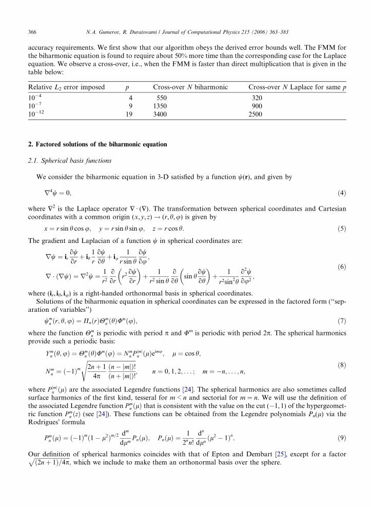
accuracy requirements. We first show that our algorithm obeys the derived error bounds well. The FMM forthe biharmonic equation is found to require about 50% more time than the corresponding case for the Laplaceequation. We observe a cross-over, i.e., when the FMM is faster than direct multiplication that is given in thetable below:

Relative L2 error imposed
p Cross-over N biharmonic Cross-over N Laplace for same p
10�4
4 550 320 10�7 9 1350 900 10�12 19 3400 2500
2. Factored solutions of the biharmonic equation

2.1. Spherical basis functions

We consider the biharmonic equation in 3-D satisfied by a function w(r), and given by

r4w ¼ 0; ð4Þ

where $2 is the Laplace operator $ Æ ($). The transformation between spherical coordinates and Cartesiancoordinates with a common origin (x,y,z)! (r,h,u) is given by

x ¼ r sin h cos u; y ¼ r sin h sin u; z ¼ r cos h. ð5Þ

The gradient and Laplacian of a function w in spherical coordinates are:

rw ¼ iroworþ ih

1

rowohþ iu

1

r sin howou

;

r � ðrwÞ ¼ r2w ¼ 1

r2

o

orr2 ow

or

� �þ 1

r2 sin ho

ohsin h

owoh

� �þ 1

r2sin2h

o2w

ou2;

ð6Þ

where (ir, ih, iu) is a right-handed orthonormal basis in spherical coordinates.Solutions of the biharmonic equation in spherical coordinates can be expressed in the factored form (‘‘sep-

aration of variables’’)

wmn ðr; h;uÞ ¼ PnðrÞHm

n ðhÞUmðuÞ; ð7Þ
where the function Hm
n is periodic with period p and Um is periodic with period 2p. The spherical harmonicsprovide such a periodic basis:

Y mn ðh;uÞ ¼ Hm

n ðhÞUmðuÞ ¼ Nmn P jmjn ðlÞeimu; l ¼ cos h;

Nmn ¼ ð�1Þm

ffiffiffiffiffiffiffiffiffiffiffiffiffiffiffiffiffiffiffiffiffiffiffiffiffiffiffiffiffiffiffiffiffiffi2nþ 1

4pðn� jmjÞ!ðnþ jmjÞ!

s; n ¼ 0; 1; 2; . . . ; m ¼ �n; . . . ; n;

ð8Þ

where P jmjn ðlÞ are the associated Legendre functions [24]. The spherical harmonics are also sometimes calledsurface harmonics of the first kind, tesseral for m < n and sectorial for m = n. We will use the definition ofthe associated Legendre function P m

n ðlÞ that is consistent with the value on the cut (�1,1) of the hypergeomet-ric function P m

n ðzÞ (see [24]). These functions can be obtained from the Legendre polynomials Pn(l) via theRodrigues� formula

P mn ðlÞ ¼ ð�1Þmð1� l2Þm=2 dm

dlmP nðlÞ; P nðlÞ ¼

1

2nn!

dn

dlnðl2 � 1Þn. ð9Þ

Our definition of spherical harmonics coincides with that of Epton and Dembart [25], except for a factorffiffiffiffiffiffiffiffiffiffiffiffiffiffiffiffiffiffiffiffiffiffiffiffiffið2nþ 1Þ=4p

p; which we include to make them an orthonormal basis over the sphere.


The dependence of the function Pn on the radial coordinate, in Eq. (7), is described by

d

drr2 d

dr

� �� nðnþ 1Þ

� �2

Pn ¼ 0. ð10Þ

This equation has four linearly independent solutions of type Pn = ra for a = n + 2, n, �n + 1, and �n � 1. Sothe biharmonic equation has the following elementary solutions:

Rmn ðrÞ ¼ am

n rnY mn ðh;uÞ; Rm

ð2ÞnðrÞ ¼ r2Rmn ðrÞ; Sm

n ðrÞ ¼ bmn r�n�1Y m

n ðh;uÞ; Smð2ÞnðrÞ ¼ r2Sm

n ðrÞ;n ¼ 0; 1; 2; . . . ; m ¼ �n; . . . ; n; ð11Þ

where amn and bm

n are some normalization constants, which can be set to unity or selected by special way tosimplify recursion and other functional relations between the elementary solutions. We note that the R-solu-tions are regular inside any finite domain, while the S-solutions have a singularity at r = 0. Function S0

ð2Þ0ðrÞ �r is finite at r = 0, while its derivatives are singular at this point. This function is proportional to the whole-space Green�s function for the biharmonic operator, G(r, r0) = |r � r0|, which satisfies

r4Gðr; r0Þ ¼ r4jr� r0j ¼ �8pdðr� r0Þ; ð12Þ

where d is the Dirac delta-function. We also note that solutions Rmn ðrÞ and Sm

n ðrÞ are solutions of the Laplaceequation, $2w = 0, in finite and infinite domains (in the latter case the origin is excluded) and the functionS0ð1Þ0ðrÞ � r�1 is proportional to the whole-space Green�s function for the Laplace operator, |r � r0|�1.

2.2. Factorization of the Green�s function

Let us start by considering factorization of the biharmonic Green�s function G(r, r0) = |r � r0|, where r0 canbe thought as the location of source, and r as the field point. Due to symmetry, the role of these points can beexchanged. Assuming r0 = |r0| > 0 consider the field of the source in the vicinity of the origin for r = |r| < r0.The Green�s function can be written as

Gðr; r0Þ ¼ ½ðr� r0; r� r0Þ�1=2 ¼ ðr2 � 2rr0 cos cþ r20Þ

1=2 ¼ r2 � 2rr0 cos cþ r20

ðr2 � 2rr0 cos cþ r20Þ

1=2

¼ ðr2 � 2rr0 cos cþ r20Þ

1

r0

X1n¼0

rr0

� �n

P nðcos cÞ; r < r0; ð13Þ

where c is the angle between vectors r and r0 and we used the generating function for the Legendre polynomials.Using the recurrence relation for the Legendre polynomials (2n + 1)lPn(l) = nPn� 1(l) + (n + 1)Pn + 1(l) thiscan be rewritten in the form

Gðr; r0Þ ¼X1n¼0

r�n�10 rnþ2

2nþ 3� r�nþ1

0 rn

2n� 1

� �P nðcos cÞ; r < r0. ð14Þ

Further, we will use the addition theorem for spherical harmonics in the form

P nðcos cÞ ¼ 4p2nþ 1

Xn

m¼�n

Y �mn ðh0;u0ÞY m

n ðh;uÞ; ð15Þ

where (h0,u0) and (h,u) are spherical polar angles of r0 and r, respectively. Substituting this into Eq. (14) andusing definitions (11), we obtain the following factorization of the Green�s function for the biharmonicequation

Gðr; r0Þ ¼ 4pX1n¼0

Xn

m¼�n

1

amn b�m

n ð2nþ 1ÞS�m

n ðr0ÞRmð2ÞnðrÞ

2nþ 3�

S�mð2Þnðr0ÞRm

n ðrÞ2n� 1

� �; r < r0. ð16Þ

Note that factorization of the Green�s function for the Laplace equation can be written in the form


jr� r0j�1 ¼ 1

r0

X1n¼0

rr0

� �n

P nðcos cÞ ¼ 4pX1n¼0

Xn

m¼�n

S�mn ðr0ÞRm

n ðrÞam

n b�mn ð2nþ 1Þ ; r < r0. ð17Þ

2.3. Reduction of the solution of biharmonic equation to solution of two harmonic equations

There are several ways how to deal with factored solutions of the harmonic and biharmonic equations. Thefirst way is to develop a translation theory for the biharmonic equation, similarly to the available theories forthe Laplace equation (e.g. [1,26,16,25]). We developed all necessary formulae to proceed in this way. However,in our study we found a second way, which simply reduces solution of the biharmonic equation to two har-monic equations with some modification of the translation operators. Computationally both methods haveabout the same complexity, and since the latter method seems simpler in terms of presentation and back-ground theory, we will proceed in this paper with it.

The method is based on the observation that any solution of the biharmonic equation w(r) can be expressedvia two independent solutions of the Laplace equation, /(r) and x(r),

wðrÞ ¼ /ðrÞ þ r2xðrÞ; r2/ðrÞ ¼ 0; r2xðrÞ ¼ 0; r4wðrÞ ¼ 0; r2 ¼ r � r. ð18Þ
Therefore, if we are able to perform operations required for the FMM for the harmonic functions andthen modify them for compositions of type (18) we can solve the biharmonic equation using the samemethod.
2.4. Function representations and translations

One of the key parts of the FMM is the translation theory. Let w(r) be an arbitrary scalar function,w : XðrÞ ! C, where XðrÞ � R3. For a given vector t 2 R3, we define a new function bw : bXðrÞ ! C, bXðrÞ �R3 such that in bXðrÞ ¼ Xðrþ tÞ the values of bwðrÞ coincide with the values of w(r + t) and treat bwðrÞ as a resultof action of translation operator TðtÞ on w(r)
bw ¼TðtÞ½w�; bwðrÞ ¼ wðrþ tÞ; r 2 bXðrÞ � R3. ð19Þ For given basis functions, a function can be represented by an infinite set of coefficients obtained by expansionover this basis. For example, if we have two expansions
/ðrÞ ¼X1n¼0

Xn

m¼�n

/mn Rm

n ðrÞ; b/ðrÞ ¼ /ðrþ tÞ ¼X1n¼0

Xn

m¼�n

b/m

n Rmn ðrÞ; ð20Þ

both expanded over the same basis fRmn ðrÞg, then it is not difficult to show that

b/m

n ¼X1n0¼0

Xn0

m0¼�n0ðRjRÞmm0

nn0 ðtÞ/m0

n0 . ð21Þ

Similar relations hold for multipole-to-multipole, or singular-to-singular (S|S), and multipole-to-local, or sin-gular-to-regular (S|R), translations. Representations of the translation operators can be found from the addi-tion theorems for the basis functions. For example, for the Laplace regular and singular basis functions wehave:

Rmn ðrþ tÞ ¼

X1n0¼0

Xn0

m0¼�n0ðRjRÞm

0mn0n ðtÞRm0

n0 ðrÞ;

Smn ðrþ tÞ ¼

X1n0¼0

Xn0

m0¼�n0ðSjRÞm

0mn0n ðtÞRm0

n0 ðrÞ; jrj < jtj;

Smn ðrþ tÞ ¼

X1n0¼0

Xn0

m0¼�n0ðSjSÞm

0mn0n ðtÞSm0

n0 ðrÞ; jrj > jtj;

ð22Þ


where t is the translation vector, and ðRjRÞm0m

n0n , ðSjRÞm0m

n0n , and ðSjSÞm0m

n0n are the four index regular-to-regular,singular-to-regular, and singular-to-singular reexpansion coefficients (sometimes called also local-to-local,multipole-to-local, and multipole-to-multipole translation coefficients).

Consider now translation of solution of the biharmonic equation represented in the form (18). We have
bwðrÞ ¼TðtÞ½wðrÞ� ¼TðtÞ½/ðrÞ þ ðr � rÞxðrÞ� ¼ /ðrþ tÞ þ ½ðrþ tÞ � ðrþ tÞ�xðrþ tÞ
¼ b/ðrÞ þ ½r2 þ 2ðr � tÞ þ t2�bxðrÞ. ð23Þ

If we want now to represent the translated solution in the form (18), i.e.,
bwðrÞ ¼ e/ðrÞ þ r2 exðrÞ; ð24Þ then we need to relate the expansion coefficients of the functions e/ðrÞ and exðrÞ and b/ðrÞ and bxðrÞ. Assumingthat all these harmonic functions are represented in the same basis, e.g. fRm
n ðrÞg and noting that exðrÞ depends

on bxðrÞ alone (the harmonic function b/ðrÞ does not contribute to the non-harmonic function r2 exðrÞ), we canwrite, taking into account the linearity of all operations considered

e/m

n ¼X1n0¼0

Xn0

m0¼�n0

b/m0

n0 þX1n0¼0

Xn0

m0¼�n0Cmm0

ð1Þnn0 ðtÞbxm0

n0 ; exmn ¼

X1n0¼0

Xn0

m0¼�n0Cmm0

ð2Þnn0 ðtÞbxm0

n0 ; ð25Þ

where Cmm0

ð1Þnn0 and Cmm0

ð2Þnn0 are entries of the matrices, which we convert a solution in the form (23) to the stan-dard form (24). As a consequence these matrices will be called ‘‘conversion matrices’’. These matrices dependon the fRm

n ðrÞg or fSmn ðrÞg. As is shown below these matrices are sparse, and the conversion operation is com-

putationally cheap compared to the translation operation.Finally, we note that in the FMM we do not translate the function, but rather change the center of

expansion. For example, by local-to-local translation from center r*1 to center r*2 we mean representationof the same function in the regular bases centered at these point respectively. It is not difficult to see thatthe expansion coefficients are related by equations of the type (21), where the translation vector is t =r*2 � r*1.

2.5. Normalized elementary solutions of the Laplace equation

The normalization factors amn and bm

n in Eq. (11) can be selected arbitrarily. For example, all of these coef-ficients can be set to be equal 1. However, we can choose these coefficients in a way that differential and trans-lation relations take some simple, or convenient for operation form, as will be done below. This follows Eptonand Dembart [25] who used the following normalization for the spherical basis functions for the Laplaceequation:

amn ¼ ð�1Þni�jmj

ffiffiffiffiffiffiffiffiffiffiffiffiffiffiffiffiffiffiffiffiffiffiffiffiffiffiffiffiffiffiffiffiffiffiffiffiffiffiffiffiffiffiffiffiffiffiffiffiffiffiffi4p

ð2nþ 1Þðn� mÞ!ðnþ mÞ!

s; bm

n ¼ ijmjffiffiffiffiffiffiffiffiffiffiffiffiffiffiffiffiffiffiffiffiffiffiffiffiffiffiffiffiffiffiffiffiffiffiffiffiffiffiffi4pðn� mÞ!ðnþ mÞ!

2nþ 1

r;

n ¼ 0; 1; . . . ; m ¼ �n; . . . ; n. ð26Þ

2.5.1. Differential relations

Let us introduce new independent variables n and g instead of Cartesian coordinates x and y according to

n ¼ xþ iy2

; g ¼ x� iy2

; x ¼ nþ g; y ¼ �iðn� gÞ. ð27Þ

We can then consider the following differential operators:

oz ¼o

oz; og ¼

o

oxþ i

o

oy; on �

o

ox� i

o

oy. ð28Þ

It is shown in Ref. [25] that the differentiation relations for normalized elementary solutions of the Laplaceequation can be written as:


ozRmn ðrÞ ¼ �Rm

n�1ðrÞ; ozSmn ðrÞ ¼ �Sm

nþ1ðrÞ;ogRm

n ðrÞ ¼ iRmþ1n�1 ðrÞ; ogSm

n ðrÞ ¼ iSmþ1nþ1 ðrÞ;

onRmn ðrÞ ¼ iRm�1

n�1 ðrÞ; onSmn ðrÞ ¼ iSm�1

nþ1 ðrÞ.ð29Þ

2.5.2. Polynomial representations

We note that the functions Rmn ðrÞ are polynomials in the variables (n,g,z). This fact is well known as the

regular solutions of the Laplace equation can be expressed via the polynomial basis. For particular normal-ization (26) the explicit expressions are the following:

Rmn ðrÞ ¼

Xn�jmjl¼0

ð�1Þlin�lrmn�l

nðnþm�lÞ=2gðn�m�lÞ=2zl

nþm�l2

� �! n�m�l

2

� �!l!

;

rmn ¼

1; nþ m ¼ 2k; k ¼ 0;�1; . . .

0; nþ m ¼ 2k þ 1; k ¼ 0;�1; . . .

ð30Þ

where we introduced symbol rmn which is 1 for even n + m and zero otherwise. This expression can be derived

by considering the differential relations (29) recursively, and taking into account that R00ðrÞ ¼ 1, or alternately

can be proved using induction and the same differential relations. Note that according to Eqs. (11) and (26) wehave

Smn ðrÞ ¼

bmn

amn

r�2n�1Rmn ðrÞ ¼ ð�1Þnþmðn� mÞ!ðnþ mÞ!r�2n�1Rm

n ðrÞ. ð31Þ

So Eqs. (27) and (30) yield the following expression for these functions

Smn ðrÞ ¼

ð�1Þnþmðn� mÞ!ðnþ mÞ!r2nþ1

Xn�jmjl¼0

ð�1Þlin�lrmn�ln

ðnþm�lÞ=2gðn�m�lÞ=2zl

nþm�l2

� �! n�m�l

2

� �!l!

; r2 ¼ 4ngþ z2. ð32Þ

2.5.3. Reexpansion coefficients

The use of the normalized basis functions yields extremely simple expressions for the reexpansion coeffi-cients entering Eq. (22) [25]:

ðRjRÞm0m

n0n ðtÞ ¼ Rm�m0

n�n0 ðtÞ; jm0j 6 n0;

ðSjRÞm0m

n0n ðtÞ ¼ Sm�m0

nþn0 ðtÞ; jm0j 6 n0; jmj 6 n;

ðSjSÞm0m

n0n ðtÞ ¼ Rm�m0

n0�n ðtÞ; jmj 6 n.

ð33Þ

2.6. Rotational-coaxial translation decomposition

If the infinite series over the basis functions of type (20) are truncated at p terms with respect to thedegree n(n = 0, . . . ,p � 1) the total number of expansion coefficients for basis functions of the first kindwill be p2. Translations using the dense truncated reexpansion matrices of size p2 · p2 performed bystraightforward way will require then O(p4) operations. This cost can be reduced to O(p3) using the rota-tional-coaxial translational decomposition (e.g. see [20,21]), since the rotations and coaxial translationscan be performed at a cost of O(p3) operations. We also note that at the rotation transforms solutionof the biharmonic equation given in form (18) remains in the same form, since the rotation transformpreserves r2.

2.6.1. Coaxial translations

A coaxial translation is translation along the polar axis or the z-coordinate axis, i.e., this is the case whenthe translation vector t = tiz, where iz is the basis unit vector along the z-axis. The peculiarity of the coaxial


translation is that it does not change the order m of the translated coefficients, and so translation can beperformed for each order independently. For example, Eq. (21) for the coaxial local-to-local translation willbe reduced to

Fig. 1.the poreferenin both

b/m

n ¼X1

n0¼jmjðRjRÞmnn0 ðtÞ/

mn0 ; m ¼ 0;�1; . . . ; n ¼ jmj; jmj þ 1; . . . ð34Þ

The three index coaxial reexpansion coefficients ðF jEÞmnn0 (F, E = S, R; m = 0, ±1, ±2, . . . , n,n 0 = |m|,|m| + 1, . . .) are functions of the translation distance t alone and can be expressed via the general reexpansioncoefficients as

ðF jEÞmnn0 ðtÞ ¼ ðF jEÞmmnn0 ðtizÞ; F ;E ¼ S;R; t P 0. ð35Þ

Using Eq. (33) we have for normalized basis functions with amn and bm

n from (26):

ðRjRÞmnn0 ðtÞ ¼ rn0�nðtÞ; n0 P jmj;ðSjRÞmnn0 ðtÞ ¼ snþn0 ðtÞ; n; n0 P jmj;ðSjSÞmnn0 ðtÞ ¼ rn�n0 ðtÞ; n P jmj;

ð36Þ

where the functions rn(t) and sn(t) are

rnðtÞ ¼ð�tÞn

n!; snðtÞ ¼

n!

tnþ1; n ¼ 0; 1; . . . ; t P 0 ð37Þ

and zero for n < 0.

2.6.2. Rotations

To perform translation with an arbitrary vector t using the computationally cheap coaxial translation oper-ators, we first must rotate the original reference frame to align the z-axis of the rotated reference frame with t,translate and then perform an inverse rotation.

An arbitrary rotation in three dimensions can be characterized by three Euler angles, or angles a, b, and cthat are simply related to them. For the forward rotation, when (h,u) are the spherical polar angles of therotated z-axis in the original reference frame, then b = h, a = u; for the inverse rotation with ðbh; buÞ the spher-ical polar angles of the original z-axis in the rotated reference frame, b ¼ bh, c ¼ bu (see Fig. 1). An importantproperty of the spherical harmonics is that their degree n does not change on rotation, i.e.,

Y mn ðh;uÞ ¼

Xn

m0¼�n

T m0mn ða; b; cÞY m0

n ðbh; buÞ; n ¼ 0; 1; 2; . . . ; m ¼ �n; . . . ; n; ð38Þ

where (h,u) and ðbh; buÞ are spherical polar angles of the same point on the unit sphere in the original and therotated reference frames, and T m0m

n ða; b; cÞ are the rotation coefficients.

yA

yyy

β

α

β

y

x

y

z

x

y

z

O

A

x

y

z

x

y

z

OA

A

γ

The figure in the left shows the transformed axes ðbx; by ;bzÞ in the original reference frame (x,y,z). The spherical polar coordinates ofint bA lying on the bz axis on the unit sphere are (b,a). The figure in the right shows the original axes (x,y,z) in the transformedce frame ðbx; by ;bzÞ. The coordinates of the point A lying on the z axis on the unit sphere are (b,c). The points O, A, and bA are the same

figures. All rotation matrices can be derived in terms of these three angles a, b, and c.


The rotation transform for solutions of the Laplace equation factored over the regular spherical basis func-tions (11) can be performed as

/ðrÞ ¼X1n¼0

Xn

m¼�n

b/m

n Rmn ðrÞ; ð39Þ

where r and r are coordinates of the same field point in the original and rotated frames, while /mn and b/m

n arethe respective expansion coefficients related as

b/m

n ¼Xn

m0¼�n

T mm0n ða; b; cÞam0

n

amn

/m0

n . ð40Þ

The same holds for the multipole expansions where in Eq. (40) we replace the normalization constantsam

n and am0n with bm

n and bm0

n , respectively.The rotation coefficients T m0m

n ða; b; cÞ can be decomposed as

T m0mn ða; b; cÞ ¼ eimae�im0cH m0m

n ðbÞ; ð41Þ

where fH m0mn ðbÞg is a dense real symmetric matrix. Its entries can be computed using an analytical expression,

or by a fast recursive procedure (see [21]), which starts with the initial value

H m00n ðbÞ ¼ ð�1Þm

0

ffiffiffiffiffiffiffiffiffiffiffiffiffiffiffiffiffiffiffiffiffiðn� jm0jÞ!ðnþ jm0jÞ!

sP jm

0 jn ðcos bÞ; n ¼ 0; 1; . . . ; m0 ¼ �n; . . . ; n ð42Þ

and further propagates values for positive m as

H m0 ;mþ1n�1 ¼ 1

bmn

1

2b�m0�1

n ð1� cos bÞH m0þ1;mn � bm0�1

n ð1þ cos bÞH m0�1;mn

h i� am0

n�1 sin bHm0mn

; ð43Þ

where n = 2,3, . . . , m 0 = �n + 1, . . . ,n � 1, m = 0, . . . ,n � 2, and amn ¼ bm

n ¼ 0 for n < |m|, and

amn ¼ a�m

n ¼

ffiffiffiffiffiffiffiffiffiffiffiffiffiffiffiffiffiffiffiffiffiffiffiffiffiffiffiffiffiffiffiffiffiffiffiffiffiffiffiffiffiffiffiffiffiffiffiffiðnþ 1þ mÞðnþ 1� mÞð2nþ 1Þð2nþ 3Þ

sfor n P jmj;

bmn ¼

ffiffiffiffiffiffiffiffiffiffiffiffiffiffiffiffiffiffiffiffiffiffiðn�m�1Þðn�mÞð2n�1Þð2nþ1Þ

q; 0 6 m 6 n;

�ffiffiffiffiffiffiffiffiffiffiffiffiffiffiffiffiffiffiffiffiffiffiðn�m�1Þðn�mÞð2n�1Þð2nþ1Þ

q; �n 6 m < 0.

8><>:ð44Þ

For negative m coefficients H m0mn ðbÞ can be found using symmetry H�m0;�m

n ðbÞ ¼ Hm0mn ðbÞ.

3. Matrices for conversion to harmonic form

In this section, we derive explicit expressions for the conversion matrices (25) in the regular and singularbases of normalized solutions of the Laplace equation. For this purpose, let us consider expansion of functionsðr � tÞRm

n ðrÞ and ðr � tÞSmn ðrÞ over the bases of functions fRm

n ðrÞg and fr2Rmn ðrÞg and fSm

n ðrÞg and fr2Smn ðrÞg,

respectively. We present the result in the form of a few lemmas.

Lemma 1. Let Rmn ðrÞ be a normalized regular elementary solution of the Laplace equation (30). Then

nRmn ðrÞ ¼ �i

nþ mþ 2

2Rmþ1

nþ1 ðrÞ �i

2zRmþ1

n ðrÞ; n ¼ 0; 1; . . . ; m ¼ �n; . . . ; n. ð45Þ


Proof. Using the polynomial representations (30) we have

nRmn ðrÞ ¼

Xn�jmjl¼0


ðnþm�lþ2Þ=2gðn�m�lÞ=2zl

ðnþm�l2Þ!ðn�m�l

2Þ!l!

¼Xn�jmjl¼0


ððnþ1Þþðmþ1Þ�lÞ=2gððnþ1Þ�ðmþ1Þ�lÞ=2zl

ðnþ1Þþðmþ1Þ�l2

� 1� �

! ðnþ1Þ�ðmþ1Þ�l2

� �!l!

¼ �iXnþ1�jmþ1j

l¼0

ð�1Þlinþ1�lrmþ1nþ1�ln



� 1� �


� �!l!

þXn�jmj

l¼nþ1�jmþ1jþ1




� 1� �


� �!l!

¼ �iXnþ1�jmþ1j

l¼0

ðnþ 1Þ þ ðmþ 1Þ � l2




� �! ðnþ1Þ�ðmþ1Þ�l

2

� �!l!

¼ �inþ mþ 2

2Rmþ1

nþ1 ðrÞ þi

2

Xnþ1�jmþ1j

l¼0




� �! ðnþ1Þ�ðmþ1Þ�l

2

� �!ðl� 1Þ!

¼ �inþ mþ 2

2Rmþ1

nþ1 ðrÞ �i

2

Xn�jmþ1j

l¼0

ð�1Þlin�lrmþ1n�l nðnþðmþ1Þ�lÞ=2gðn�ðmþ1Þ�lÞ=2zlþ1

nþðmþ1Þ�l2

� �! n�ðmþ1Þ�l

2

� �!l!

¼ �inþ mþ 2

2Rmþ1

nþ1 ðrÞ �i

2zRmþ1

n ðrÞ. �

Corollary 2. Let Rmn ðrÞ be a normalized regular elementary solution of the Laplace equation (30). Then

gRmn ðrÞ ¼ �i

n� mþ 2

2Rm�1

nþ1 ðrÞ �i

2zRm�1

n ðrÞ; n ¼ 0; 1; . . . ; m ¼ �n; . . . ; n. ð46Þ

Proof. According to Eqs. (11) and (26) we have for complex conjugate

Rmn ðrÞ ¼ ð�1ÞmR�m

n ðrÞ. ð47Þ
Since g ¼ n (see Eq. (27)) we obtain using Lemma 1
gRmn ðrÞ ¼ gRm

n ðrÞ ¼ ð�1ÞmnR�mn ðrÞ ¼ ð�1Þm �i

n� mþ 2

2R�mþ1

nþ1 ðrÞ �i

2zR�mþ1

n ðrÞ� �

¼ ð�1Þm in� mþ 2

2ð�1Þm�1Rm�1

nþ1 ðrÞ þi

2zð�1Þm�1Rm�1

n ðrÞ� �

¼ �in� mþ 2

2Rm�1

nþ1 ðrÞ �i

2zRm�1

n ðrÞ. �


zRmn ðrÞ ¼ �

1

2nþ 1ðnþ mþ 1Þðn� mþ 1ÞRm

nþ1ðrÞ þ r2Rmn�1ðrÞ

�;

n ¼ 0; 1; . . . ; m ¼ �n; . . . ; n. ð48Þ

Proof. Using the following identity for the associated Legendre functions

lP mn ðlÞ ¼

nþ m2nþ 1

P mn�1ðlÞ þ

n� mþ 1

2nþ 1P m

nþ1ðlÞ ð49Þ


and definition of the basis functions (11) we can find

zRmn ðrÞ ¼ am

n N mn eimurnþ1lP jmjn ðlÞ ¼ am

n N mn eimurnþ1 nþ jmj

2nþ 1P jmjn�1ðlÞ þ

n� jmj þ 1

2nþ 1P jmjnþ1ðlÞ

� �¼ 1

2nþ 1ðnþ jmjÞ am

n N mn

amn�1N m

n�1

r2Rmn�1ðrÞ þ ðn� jmj þ 1Þ

amð1ÞnN m

n

amnþ1N m

nþ1

Rmnþ1ðrÞ

� �. ð50Þ

Since

amn N m

n ¼ð�1Þnþmi�jmj

ðnþ jmjÞ! ; ð51Þ

we obtain the statement of the lemma. h


ðr � tÞRmn ðrÞ ¼ �

ðitx þ tyÞðnþ mþ 2Þðnþ mþ 1ÞRmþ1nþ1 ðrÞ

2ð2nþ 1Þ

� ðitx � tyÞðn� mþ 2Þðn� mþ 1ÞRm�1nþ1 ðrÞ þ 2tzðnþ mþ 1Þðn� mþ 1ÞRm

nþ1ðrÞ2ð2nþ 1Þ

þ r2½ðitx þ tyÞRmþ1n�1 ðrÞ þ ðitx � tyÞRm�1

n�1 ðrÞ � 2tzRmn�1ðrÞ�

2ð2nþ 1Þ . ð52Þ

Proof. Follows from Eqs. (45)–(48) and

ðr � tÞRmn ðrÞ ¼ ðxtx þ yty þ ztzÞRm

n ðrÞ ¼ ½ðtx � ityÞnþ ðtx þ ityÞgþ tzz�Rmn ðrÞ. � ð53Þ

Lemma 5. Let Smn ðrÞ be a normalized singular elementary solution of the Laplace equation (30). Then

ðr � tÞSmn ðrÞ ¼

ðitx þ tyÞðn� m� 1Þðn� mÞSmþ1n�1 ðrÞ

2ð2nþ 1Þ

þ ðitx � tyÞðnþ m� 1Þðnþ mÞSm�1n�1 ðrÞ þ 2tzðn� mÞðnþ mÞSm

n�1ðrÞ2ð2nþ 1Þ

� r2½ðitx þ tyÞSmþ1nþ1 ðrÞ þ ðitx � tyÞSm�1

nþ1 ðrÞ � 2tzSmnþ1ðrÞ�

2ð2nþ 1Þ . ð54Þ

Proof. Follows from Eqs. (31) and (52). h

Lemma 6. Let b/m

n , bxmn , e/m

n , and exmn be coefficients of expansions of harmonic functions b/ðrÞ, bxðrÞ, e/ðrÞ, andexðrÞ over the normalized regular basis fRm

n ðrÞg that satisfy relation

e/ðrÞ þ r2 exðrÞ ¼ b/ðrÞ þ ½r2 þ 2ðr � tÞ þ t2�bxðrÞ. ð55Þ

Then

e/m

n ¼ b/m

n þ t2 bxmn �ðitx þ tyÞðnþ mÞðnþ m� 1Þbxm�1

n�1

2n� 1

� ðitx � tyÞðn� mÞðn� m� 1Þbxmþ1n�1 þ 2tzðnþ mÞðn� mÞbxm

n�1

2n� 1;

exmn ¼ bxm

n þ1

2nþ 3½ðitx þ tyÞbxm�1

nþ1 þ ðitx � tyÞbxmþ1nþ1 � 2tz bxm

nþ1�.

ð56Þ


Proof. Follows from Eqs. (52) and (55) by grouping the terms multiplying functions Rmn ðrÞ and r2Rm

n ðrÞ andcomparing coefficients. h

Lemma 7. Let b/m

n , bxmn , e/m

n , and exmn be coefficients of expansions of harmonic functions b/ðrÞ, bxðrÞ, e/ðrÞ, andexðrÞ over the normalized singular basis fSm

n ðrÞg that satisfy relation (55). Then:

e/m

n ¼ b/m

n þ t2 bxmn þðitx þ tyÞðn� mþ 1Þðn� mþ 2Þbxm�1

nþ1

2nþ 3

þ ðitx � tyÞðnþ mþ 1Þðnþ mþ 2Þbxmþ1nþ1 þ 2tzðn� mþ 1Þðnþ mþ 1Þbxm

nþ1

2nþ 3;

exmn ¼ bxm

n �1

2n� 1½ðitx þ tyÞbxm�1

n�1 þ ðitx � tyÞbxmþ1n�1 � 2tz bxm

n�1�.

ð57Þ

Proof. Follows from Eqs. (54) and (55) by grouping the coefficients of the functions Smn ðrÞ and r2Sm

n ðrÞ andcomparison of the coefficients. h

Relations (56) and (57) in fact determine the entries of the conversion matrices (25). These matrices aresparse, since only 4 elements bxm

n are needed to determine exmn and e/m

n . Note that in the FMM where the trans-lation is decomposed into rotation and coaxial translation operations, the conversion operation can be per-formed for a lower cost after the coaxial translation. Conversion formulae for coaxial translation can beobtained easily from Eqs. (56) and (57) by setting tx = ty = 0, tz = t. So we have for expansions over the regularbasis fRm

n ðrÞg:

e/m

n ¼ b/m

n þ t2 bxmn � 2t

ðnþ mÞðn� mÞ2n� 1

bxmn�1; exm

n ¼ bxmn �

2t2nþ 3

bxmnþ1. ð58Þ

For expansion over the singular basis fSmn ðrÞg we have:

e/m

n ¼ b/m

n þ t2 bxmn þ 2t

ðnþ mþ 1Þðn� mþ 1Þ2nþ 3

bxmnþ1; exm

n ¼ bxmn þ

2t2n� 1

bxmn�1. ð59Þ

4. Polyharmonic equations

While we will not pursue this here, the method presented above can be easily extended to solution of poly-harmonic equations of type

r2kw ¼ 0; k ¼ 3; 4; . . . ð60Þ

The Green�s functions of these functions are often used in radial-basis function interpolation. In this case solu-tion in spherical coordinates can be represented in the form

wðrÞ ¼ /1ðrÞ þ r2/2ðrÞ þ r4/3ðrÞ þ � � � þ r2k�2/kðrÞ ¼Xk

j¼1

r2j�2/jðrÞ; ð61Þ

where /j(r), j = 1, . . . ,k. The translation operator acts on this solution as follows:

bwðrÞ ¼TðtÞ½wðrÞ� ¼TðtÞXk

j¼1

ðr � rÞ2j�2/jðrÞ" #

¼Xk

j¼1

½ðrþ tÞ � ðrþ tÞ�2j�2b/jðrÞ

¼Xk

j¼1

½r2 þ 2ðr � tÞ þ t2�j�1b/jðrÞ; ð62Þ

where we used the binomial expansion. As shown above the conversion operator provides a transform, whichcan be written as:


½r2 þ 2ðr � tÞ þ t2�b/jðrÞ ¼ Uð1;1Þj ðrÞ þ r2Uð1;2Þj ðrÞ;½r2 þ 2ðr � tÞ þ t2�2b/jðrÞ ¼ ½r2 þ 2ðr � tÞ þ t2�Uð1;1Þj ðrÞ þ r2½r2 þ 2ðr � tÞ þ t2�Uð1;2Þj ðrÞ

¼ Uð2;1Þj ðrÞ þ r2Uð2;2Þj ðrÞ þ r4Uð2;2Þj ðrÞ;

..

.

½r2 þ 2ðr � tÞ þ t2�j�1b/jðrÞ ¼Xj

l¼1

r2l�2Uðj�1;lÞj ðrÞ;

ð63Þ

where Uðj�1;lÞj ðrÞ are harmonic functions. So we can rewrite Eq. (62) as

bwðrÞ ¼Xk

j¼1

Xj

l¼1

r2l�2Uðj�1;lÞj ðrÞ ¼

Xk

l¼1

r2l�2Xk

j¼l

Uðj�1;lÞj ðrÞ ¼

Xk

l¼1

r2l�2e/lðrÞ; ð64Þ

where

e/lðrÞ ¼Xk

j¼l

Uðj�1;lÞj ðrÞ. ð65Þ

Eq. (64) represents the translated solution in the same form as the original solution (compare with Eq. (61)).Therefore, solution of k-harmonic equation can be reduced to solution of k Laplace equations (e.g. the trihar-monic equation solution can be expressed in terms of three harmonic functions), with modification of thetranslation operators, which include multiplications by sparse conversion matrices. Such multiplicationscan be greatly simplified using the rotational-coaxial translation decompositions.

5. Fast multipole method

5.1. Mapping a real biharmonic function to a complex harmonic function

A nice property of the harmonic and biharmonic equations is that they can be solved for both real andcomplex-valued functions. If the function is complex valued one can simply solve the problem for real andimaginary parts. In this case one can rewrite the equations in terms of real spherical harmonics and translationoperators, which, however, makes the formulae more involved. So it is preferable to operate with complexfunctions. In terms of the use of the FMM we found that it only needs to be slightly modified, so anFMM matrix–vector product routine for the complex Laplace equation can be used for the biharmonic equa-tion for real valued functions, which is the practical case typically encountered.

To show how this works, let us first consider solution of the Laplace equation for real valued function /(r).Assume that this function is expanded over the regular basis according to Eq. (20). Then due to the property(47) of normalized spherical basis functions we have

/ðrÞ ¼X1n¼0

Xn

m¼�n

/mn Rm

n ðrÞ ¼X1n¼0

Xn

m¼�n

ð�1Þm/mn R�m

n ðrÞ ¼X1n¼0

Xn

m¼�n

ð�1Þm/�mn Rm

n ðrÞ. ð66Þ

Since /ðrÞ ¼ /ðrÞ, comparing this with Eq. (20) and taking into account uniqueness of the expansion over thebasis, we can find that expansion coefficients of real functions satisfy relation

/mn ¼ ð�1Þm/�m

n ; n ¼ 0; 1; . . . ; m ¼ �n; . . . ; n. ð67Þ

Now, let us consider a complex valued harmonic function

WðrÞ ¼ /ðrÞ þ ixðrÞ; Wmn ¼ /m

n þ ixmn ; ð68Þ

where / and x are real, and functions W, /, and x can be expanded over basis fRmn ðrÞg with coefficients Wm

n ,/m

n , and xmn . We have then relation (67), which is valid for coefficients of real functions /m

n and xmn :

Fig. 3.transla


Wmn � ixm

n ¼ /mn ¼ ð�1Þm/�m

n ¼ ð�1ÞmðW�mn þ ix�m

n Þ ¼ ð�1ÞmW�mn þ ixm

n ;

Wmn � /m

n ¼ ixmn ¼ �ð�1Þmðix�m

n Þ ¼ �ð�1ÞmðW�mn � /�m

n Þ ¼ �ð�1ÞmW�mn þ /m

n .ð69Þ

This yields

/mn ¼

1

2½Wm

n þ ð�1ÞmW�mn �; xm

n ¼1

2i½Wm

n � ð�1ÞmW�mn �. ð70Þ

It is not difficult to check that this relation holds also if Wmn , /m

n , and xmn are expansion coefficients of W, /, and

x over basis fSmn ðrÞg. Thus, if harmonic function W(r) is known via its expansion coefficients, then expansion

coefficients of its real and imaginary parts can be easily retrieved. This maps harmonic function W(r) to bihar-monic function w(r) represented as Eq. (18).

As the translation process of biharmonic function is concerned, we, first, perform translation of coefficientsWm

n to bWm

n using translation operators for the Laplace equation, second, we determine b/m

n and bxmn from bWm

n

according to Eq. (70), third, we convert b/m

n and bxmn to e/m

n and exmn according to Eqs. (56) and (57), and, finally,

we form eWm

n ¼ e/m

n þ iexmn , which is a representation of the translated biharmonic function. This is shown on a

flow chart in Fig. 2.As mentioned above the conversion operator can be simplified in the case of coaxial translation. The flow

chart corresponding to this case is shown in Fig. 3.

5.2. Basic FMM algorithm

Generally speaking any solver for Laplace equation can be adjusted to solve the biharmonic equation, assoon as translation operators are modified according to the scheme in Fig. 2. We will not present details of thebasic FMM algorithm, which are well described in the original papers of Greengard, Rokhlin, and others[1,26]. Our implementation of the Laplace solvers is described in [21], where we also provided operationaland memory complexity, error analysis, and comparison of two fastest versions of the FMM currentlyavailable.

1. Translate coefficients of complex

harmonic function

2. Decompose coefficients of complex function

3. Convert coefficients4. Compose coefficients ofcomplex harmonic function

Complex harmonic representation


1. Translate coefficients of complex

harmonic function


3. Convert coefficients4. Compose coefficients ofcomplex harmonic function



Fig. 2. A flow chart for translation of solutions of the biharmonic equation using complex harmonic representation.

1. Rotate coefficients of complex

harmonic function


4. Coaxially convert coefficients

5. Compose coefficients ofcomplex harmonic function



2. Coaxially translatecoefficients of complex

harmonic function

6. Rotate back coefficients of complex

harmonic function

1. Rotate coefficients of complex

harmonic function


4. Coaxially convert coefficients

5. Compose coefficients ofcomplex harmonic function



2. Coaxially translatecoefficients of complex

harmonic function

6. Rotate back coefficients of complex

harmonic function

A flow chart for translation of solutions of the biharmonic equation using complex harmonic representation and rotation-coaxialtion decomposition.


The algorithm consists of two main parts: the preset step, which includes building the data structure (build-ing and storage of the neighbor lists, etc.) and precomputation and storage of all translation data. The datastructure is generated using the bit interleaving technique described in [27], which enables spatial ordering,sorting, and bookmarking. While the algorithm is designed for two independent data sets (N arbitrary locatedsources and M arbitrary evaluation points), for the current tests we used the same source and evaluation setsof length N, which is also called the problem size. For a problem size N, the cost of building the data structurebased on spatial ordering is O(N logN), where the asymptotic constant is much smaller than the constants inthe O(N) asymptotics of the main algorithm. The number of levels could be arbitrarily set by the user or foundautomatically based on the clustering parameter (the maximum number of sources in the smallest box) foroptimization of computations of problems of different size.

Fig. 4 shows the main steps of the standard FMM, assuming that the preset part is performed initially. HereSteps 1 and 2 constitute the upward pass in the box hierarchy, Steps 3–5 form the downward pass and Steps 6and 7 relate to final summation. The upward pass is performed for boxes in the source hierarchy, while thedownward pass and final summation are performed for the evaluation hierarchy. By ‘‘near neighborhood’’we mean the box itself and its immediate neighbors, which in 3D consists of 27 boxes for a box not adjacentto the boundary, and the ‘‘far neighbors’’, are boxes from the parent near neighborhood (of the size of thegiven box), which do not belong to the close neighborhood. The number of such boxes is 189 in case thebox is sufficiently separated from the boundary of the domain.

5.3. Numerical tests

To validate the theory and conduct some performance tests we developed software for the FMM for solu-tions of the biharmonic equation. The code was developed in Fortran 95 and compiled using the Compaq 6.5Fortran compiler. All computations were performed in double precision. The CPU time measurements wereconducted on a 3.2 GHz dual Intel Xeon processor with 3.5 GB RAM. In the tests we studied a benchmarkcase where N sources (Green�s functions for the biharmonic equation (16)) are uniformly randomly distributedinside a unit cube. The intensities of the sources generally were assigned randomly, while for consistency oferror measurements we often used sources of the same intensity.

5.3.1. Computation of errors

To validate accuracy of the FMM we measured the relative error in the L2 norm evaluated over M randompoints in the domain

�2 ¼PM

j¼1jwexactðrjÞ � wapproxðrjÞj2PMj¼1jwexactðrjÞj2

" #1=2

; ð71Þ

where wexact(r) and wapprox(r) are the exact and approximate solutions of the problem.The exact solution was computed by straightforward summation of the source potentials (1). This method

is acceptable for relatively low M, while for larger M the computations become unacceptably slow, and the

1. Get S-expansion coefficients(directly)

2. Get S-expansion coefficients from children

(S|S translation)

Level lmax

3. Get R-expansion coefficients from far neighbors

(S|R translation)

Level 2

4. Get R-expansioncoefficients from far neighbors

(S|R translation)

6. Evaluate R-expansions (directly)

7. Sum sourcesin close neighborhood

(directly)

Start

End

Level lmaxLevel lmax

5. Get R-expansioncoefficients from parents

(R|R translation)

Levels lmax-1,…, 2 Levels 3,…,lmax

1. Get S-expansion coefficients(directly)

2. Get S-expansion coefficients from children

(S|S translation)

Level lmax

3. Get R-expansion coefficients from far neighbors

(S|R translation)

Level 2

4. Get R-expansioncoefficients from far neighbors

(S|R translation)

6. Evaluate R-expansions (directly)

7. Sum sourcesin close neighborhood

(directly)

Start

End

Level lmaxLevel lmax

5. Get R-expansioncoefficients from parents

(R|R translation)

Levels lmax-1,…, 2 Levels 3,…,lmax

Fig. 4. A flow chart of the standard FMM.


error can be measured by evaluation of the errors at smaller number of the evaluation points. We found exper-imentally that the relative L2-norm error evaluated over 100 points is quite close to the error evaluated overthe full set for N < 100,000. So we used this partial error measure to evaluate the computation error.

The error of the FMM depends on several factors. It is mainly influenced by the truncation number, p,which is the number of terms in the outer summation (n = 0, . . . ,p � 1). We note that the total number ofexpansion coefficients for a single harmonic function for a truncation number p is p2, since the order changesas m = �n, . . . ,n, in the truncated series representation of a harmonic function. We used this truncation forrepresentation of harmonic functions /(r) and x(r) in decomposition of the biharmonic function w(r) (seeEq. (18)), and accordingly we truncated all translation operators to matrices, where the maximum order m

and degree n are p � 1.Fig. 5 shows the dependence of the relative L2 error evaluated over M = 100 points on p for fixed N. It is

seen that for larger p this error decays exponentially. However even p � 4 provide a reasonably small error,which might be sufficient for computation of some practical problems. It is noticeable that �2 almost doesnot depend on N. This is shown in Fig. 6. This is due to the growth of the norm of function w(r) (see Eq. 1) withN. If one is interested with absolute error in L1 norm, then to keep it constant for increasing N we shouldincrease p � logN. We conducted corresponding numerical experiments for harmonic functions, which arereported in [21].

5.3.2. Performance

Once some truncation number providing sufficient accuracy is selected, the FMM should be optimized interms of selection of optimum maximum level of space subdivision, lmax. As is discussed in [21], for the Laplaceequation lmax is proportional to logN and, in fact, for fixed p theoretically should depend only on the cluster-ing parameter s, which is the maximum number of sources in the smallest box of space subdivision. This is alsotrue for the biharmonic equation. Accordingly, we varied this parameter to achieve the minimum CPU timefor each case reported.

Fig. 7 shows the dependences of the CPU time required for the ‘‘run’’ part of the FMM algorithm. It is seenthat independently on p the complexity of the FMM is linear with respect to N, which is consistent with thetheory. The direct summation method scaled as O(N2). We used the same algorithm for the direct summationas that used in the computation of local sums in the FMM. In this routine we have two nested loops, with theGreen�s function matrix entries computed in the inner loop. We note that the break-even points, N = N* (the

1.E-15

1.E-12

1.E-09

1.E-06

1.E-03

1.E+00

0 5 10 15 20 25

Truncation Number, p

Rel

ativ

e L 2

Err

or

FMMN=131072lmax = 4

y=ab-p

Fig. 5. A dependence of the relative FMM error in the L2 norm (�2) computed over 100 random points on the truncation number p forN = 217 = 131,072 sources of equal intensity distributed uniformly randomly inside a unit cube. The maximum level of space subdivisionlmax = 4. For p > 6 the error can be approximated by dependence �2 = ab�p.

1.E-15

1.E-12

1.E-09

1.E-06

1.E-03

1.E+03 1.E+04 1.E+05 1.E+06 1.E+07

Number of Sources, N

Rel

ativ

e L 2

Err

or

p=4

p=9

p=19

Fig. 6. Dependences of the relative error �2 on the size of the problem for different truncation numbers. Computations made for settingsdescribed in Figs. 5 and 7. lmax was selected for the optimum CPU time of the algorithm.

1.E-02

1.E-01

1.E+00

1.E+01

1.E+02

1.E+03

1.E+03 1.E+04 1.E+05 1.E+06 1.E+07


CP

U T

ime

(s)

Directp=4p=9p=19

y=axy=bx2

Direct

FMM

p=4

9

19

Fig. 7. Dependences of the CPU (run) time, measured on Intel Xeon 3.2 GHz processor (3.5 GB RAM) on the size of the problem.Computations performed using the direct summation and the FMM with different truncation numbers shown near the curves. Sources(Green�s function for biharmonic equation) of equal intensities are distributed uniformly randomly inside a cube. The series of the FMMdata are connected with the solid lines. The dashed lines show asymptotic complexities of the algorithms at large N.


points at which the CPU time of the direct method coincides with the CPU time of the FMM) depend on thetruncation number (or on the accuracy of computations) and on the implementation of the algorithm. In ourimplementation of the 3D biharmonic solver we obtained N* = 550 for p = 4, N* = 1350 for p = 9, andN* = 3550 for p = 19. Note that we obtained the break-even numbers N* = 320, 900, and 2500 for p = 4, 9,and 19 using the same coaxial translation method for the Laplace equation for real functions [21].

Fig. 8 shows the CPU times required for the ‘‘run’’ parts of the FMM algorithm for the Laplace andbiharmonic equations (both for real functions). It is seen that, in fact solution of the biharmonic equationis faster than just sum of two Laplace equations. There are a couple of reasons for that. First, in both caseswe use the same data structure and the translation operators for a single Laplace equation can be used for

1.E-02

1.E-01

1.E+00

1.E+01

1.E+02

1.E+03

1.E+03 1.E+04 1.E+05 1.E+06 1.E+07Number of Sources, N

CP

U T

ime

(s)

DirectLaplace, runBiharmonic, runPreset

y=ax

y=bx2

Direct

FMM (run)

FMM (preset)

p=9

Fig. 8. A comparison of the CPU times for the direct summation (the dark rhombs), the ‘‘run’’ parts of the FMM algorithms for theLaplace (the triangles) and the biharmonic (the squares) equations, and the ‘‘preset’’ step of the FMM algorithm (the dark discs). TheFMM for the Laplace and biharmonic equation was employed with p = 9 and the same data structure. Other settings are the same as inFig. 7.


the biharmonic equation. Second, even though the translation for the biharmonic equation more costly thanfor the Laplace equation, the direct summation in the neighborhoods of the evaluation points for the bothequations have the same cost. Therefore translations only take a part of the CPU time. Moreover, the opti-mization of the algorithm leads to balancing of the costs of translations and direct summations. So, theo-retically, one can expect only 50% (not 100%) CPU time increase for solution of the biharmonic equationcompared to the Laplace equation. These numbers are close to that we observed in actual computations forthe maximum difference in the CPU times, e.g. for N = 219 the increase of the CPU time was 59%, and forN = 220 we had 36% increase (note that the ratio of the CPU times varies, due to the discrete change of themaximum level of space subdivision, which means that the translations may constitute not exactly 50% ofthe run time of the algorithm).

Fig. 8 also shows the time needed to preset the FMM. As we mentioned above this step should be per-formed only once for a given set of source and evaluation points and includes setting of the data structureand precomputation of the translation operators. Even if it performed every time when the FMM run routineis called, it does not substantially affect the execution time, since it may contribute only 10% or so to the totalcomputation time (so the FMM can be used for computation of dynamic system with moving sources). Thegraph of the preset time shows jumps, which are related to the change of the maximum level of space subdi-vision. Almost the same CPU time is required to preset the FMM for different number of data points and thesame lmax.

Memory issues. The memory required for an efficient FMM substantially depends on the resources available,since the speed can be substantially increased using extensive precomputations, while on the other hand thememory can be substantially reduced when resources are constrained to fit what is available trading speedfor memory savings [21]. The speed also can be traded for memory by running the code in a non-optimal setting(say with a reduced number of levels below what is optimal). In the present implementation we used precom-putation of the translation operators in the FMM preset step to reduce the run time. As it is seen from Fig. 9 thiscreates a substantial memory overhead for relatively small N (memory consumption without this overhead isshown by the triangles).

Note, that the major memory consumption is due to the storage of sets of the sources, evaluation points(which, generally speaking can be different from the sources), the input and output vectors (source strengthsand the values of the sum), and due to the storage of the expansion coefficients. This memory for double pre-cision (8 byte) real numbers can be estimated as

1.E-01

1.E+00

1.E+01

1.E+02

1.E+03

1.E+04

1.E+03 1.E+04 1.E+05 1.E+06 1.E+07


Mem

ory

(MB

)

Biharmonic Faster/Higher Memory

Biharmonic Slower/Lower Memory

Laplace Faster/Higher Memory

Laplace Slower/Lower Memoryy=ax

p=9

Fig. 9. CPU memory required for computation of the problem for Laplace and biharmonic equations with the same lmax (p = 9). Thecircles correspond to the faster version of the FMM, which requires precomputation and storage of translation operators, and which CPUtime is shown in Fig. 8.


N bytes 8 � 3N þ 3N þ N þ N þ 8

72 � N

s� 2p2

� �¼ 64N � 1þ 4p2

7s

� �. ð72Þ

For the Laplace equation the coefficient of p2 should be two times smaller (due to the twice shorter represen-tation). In this estimate N/s is the number of boxes, since the optimal performance should be achieved at somevalue of clustering parameter s which does not depend on N, or varies slowly with N. This shows also that forfixed p the memory grows linearly with N, which is consistent with the numerical observations. Note that thestaircase shape of the graphs are related to the changes of lmax (in fact for uniform distributions one should use8lmax instead of N/s in Eq. (72)).

6. Conclusions

We developed a fast method to solve a biharmonic equation in three dimensions based on the FMM for theLaplace equation. The method modifies translation operators and such modifications can be used with any sol-ver of the Laplace equation employing translations or reexpansions including tree codes and various versions ofthe FMM. Numerical tests show good performance in terms of accuracy and speed.

References

[1] L. Greengard, V. Rokhlin, A fast algorithm for particle simulations, J. Comput. Phys. 73 (1987) 325–348.[2] L.E. Malvern, Introduction to the Mechanics of a Continuous Medium, Prentice-Hall, Englewood Cliffs, NJ, 1969.[3] N. Nishimura, Fast multipole accelerated boundary integral equation methods, Appl. Mech. 55 (2002) 299–324.[4] Y. Fu, K.J. Klimkowski, G.J. Rodin, E. Berger, J.C. Browne, J.K. Singer, R. Van de Geijn, K.S. Vemaganti, A fast solution method

for three-dimensional many-particle problems of linear elasticity, Int. J. Numer. Meth. Eng. 42 (1998) 1215–1229.[5] F. Chen, D. Suter, Fast evaluation of vector splines in three dimensions, J. Comput. 61 (3) (1998) 189–213.[6] V. Popov, H. Power, An O(N) Taylor series multipole boundary element method for three-dimensional elasticity problems, Eng.

Anal. Boundary Elem. 25 (2001) 7–18.[7] L. Ying, G. Biros, D. Zorin, H. Langston, A new parallel kernel-independent fast multipole method, ACM SC�03, Phoenix, AZ, 2003.[8] A.S. Sangani, G. Mo, An O(N) algorithm for Stokes and Laplace interactions of particles, Phys. Fluid 8 (1996) 1990–2010.[9] J. Happel, H. Brenner, Low Reynolds Number Hydrodynamics, Prentice-Hall, Englewood Cliffs, NJ, 1965 (reprinted by Martinus

Nijhoff, Kluwer Academic Publishers, 1983).[10] A. Greenbaum, L. Greengard, A. Mayo, On the numerical solution of the biharmonic equation in the plane, Physica D 60 (1992) 216–

225.


[11] L. Greengard, M.C. Kropinski, A. Mayo, Integral methods for Stokes flow and isotropic elasticity in the plane, J. Comput. Phys. 125(1996) 403–414.

[12] Y. Fu, G.J. Rodin, Fast solution method for three-dimensional Stokesian many-particle problems, Commun. Numer. Meth. Eng. 16(2000) 145–149.

[13] K. Yoshida, Applications of Fast Multipole Method to Boundary Integral Equation Method, Ph.D. Thesis, Department of GlobalEnvironment Engineering, Kyoto University, Japan, 2001.

[14] K. Yoshida, N. Nishimura, S. Kobayashi, Application of new fast multipole boundary integral equation method to elastostatic crackproblems in three dimensions, J. Struct. Eng. JSCE 47A (2001) 169–179.

[15] L. Greengard, V. Rokhlin, A new version of the fast multipole method for the Laplace equation in three dimensions, Acta Numer. 6(1997) 229–269.

[16] H. Cheng, L. Greengard, V. Rokhlin, A fast adaptive multipole algorithm in three dimensions, J. Comput. Phys. 155 (1999) 468–498.[17] J. Duchon, Splines minimizing rotation-invariant semi-norms in Sobolev spaces, in: W. Schempp, K. Zeller (Eds.), Constructive

Theory of Functions of Several Variables, Lecture Notes in Mathematics, vol. 571, Springer-Verlag, Berlin, 1977, pp. 85–100.[18] J.C. Carr, R.K. Beatson, J.B. Cherrie, T.J. Mitchell, W.R. Fright, B.C. McCallum, T.R. Evans, Reconstruction and representation of

3D objects with radial basis functions, ACM SIGGRAPH 2001, Los Angeles, CA, 2001, pp. 67–75.[19] J.B. Cherrie, R.K. Beatson, G.N. Newsam, Fast evaluation of radial basis functions: methods for generalised multiquadrics in Rn,

SIAM J. Sci. Comput. 23 (5) (2002) 1549–1571.[20] C.A. White, M. Head-Gordon, Rotation around the quartic angular momentum barrier in fast multipole method calculations, J.

Chem. Phys. 105 (12) (1996) 5061–5067.[21] N.A. Gumerov, R. Duraiswami, Comparison of the Efficiency of Translation Operators Used in the Fast Multipole Method for the

3D Laplace Equation, University of Maryland, Department of Computer Science, Technical Report CS TR#-4701, UMIACS TR# –2005-09, 2005.

[22] S. Kim, Stokes flow past three spheres: an analytic solution, Phys. Fluid 30 (1987) 2309–2314.[23] A.V. Filippov, Phoretic motion of arbitrary clusters of N spheres, J. Colloid Interf. Sci. 241 (2001) 479–491.[24] M. Abramowitz, I.A. Stegun, Handbook of Mathematical Functions, National Bureau of Standards, Washington, DC, 1964.[25] M.A. Epton, B. Dembart, Multipole translation theory for the three-dimensional Laplace and Helmholtz equations, SIAM J. Sci.

Comput. 4 (16) (1995) 865–897.[26] L. Greengard, The Rapid Evaluation of Potential Fields in Particle Systems, MIT Press, Cambridge, MA, 1988.[27] N.A. Gumerov, R. Duraiswami, Fast Multipole Methods for the Helmholtz Equation in Three Dimensions, Elsevier, Amsterdam,

2005.

Documents

Fast multipole method for the biharmonic equation in three dimensions