Embed Size (px)
Citation preview
Algorithmic number theory, edited by Buhler and Stevenhagen, to appear.
FAST MULTIPLICATION AND ITS APPLICATIONS
DANIEL J. BERNSTEIN
Abstract. This survey explains how some useful arithmetic operations canbe sped up from quadratic time to essentially linear time.
§2. Product:the FFT case
��
§13. Sum of fractions
§3. Product:extension
��
§11. Matrix product
��
§14. Fraction fromcontinued fraction
§4. Product:zero-padding and
localization
��
55kkkkkkkkkkkkk
§12. Product tree
::uuuuuuuuuuuuuuuuuuuuuuuuuu
$$IIIIIIIIIIIIIIIIIIIIIIIIII
��
55jjjjjjjjjjjjjjjj §20. Small factorsof a sequence
§5. Product:completion
��
§15. Exponential:the short case
��
§19. Small factorsof a product
OO
§6. Reciprocal
��
§16. Exponential:the general case
§18. Remainder tree
OO
��§7. Quotient
��
// §17. Quotientand remainder
��
55jjjjjjjjjjjjjjjj
§23. Interpolator
§8. Logarithm:the series case
��
§21. Continued fractionfrom fraction
// §22. Greatestcommon divisor
��
OO
§9. Exponential:the series case
// §10. Power:the series case
§24. Coprime base
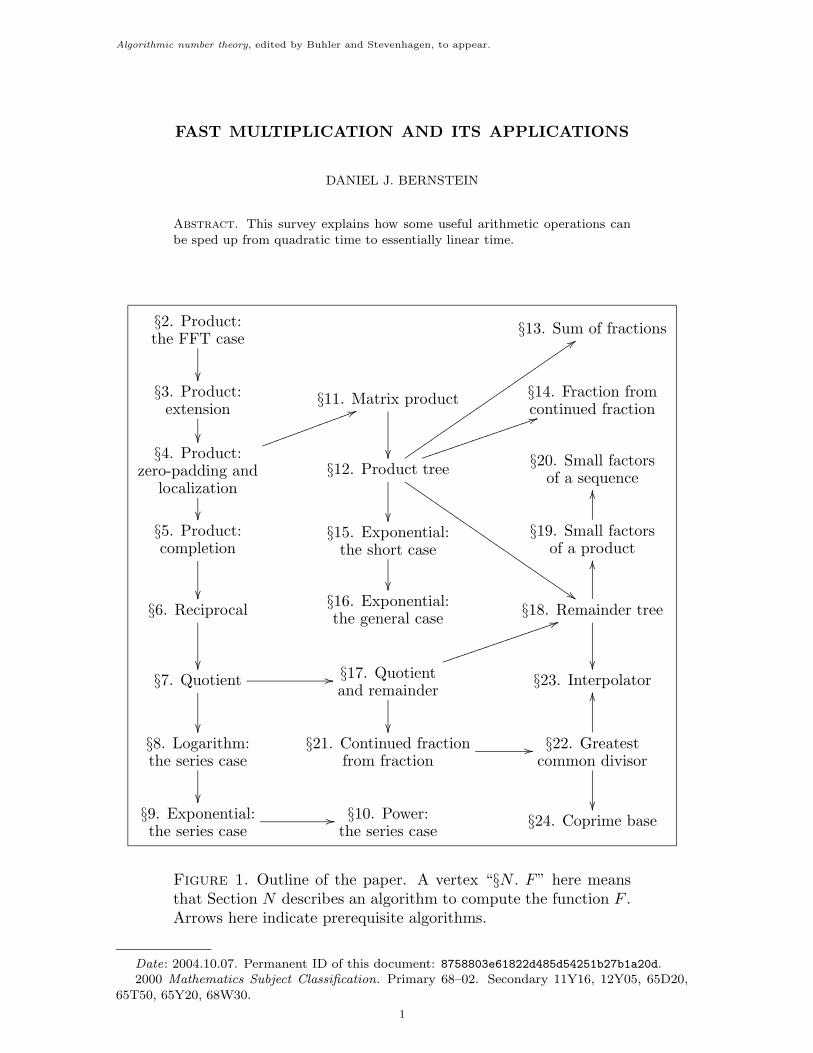
Figure 1. Outline of the paper. A vertex “§N . F” here meansthat Section N describes an algorithm to compute the function F .Arrows here indicate prerequisite algorithms.
Date: 2004.10.07. Permanent ID of this document: 8758803e61822d485d54251b27b1a20d.2000 Mathematics Subject Classification. Primary 68–02. Secondary 11Y16, 12Y05, 65D20,
65T50, 65Y20, 68W30.
1
2 DANIEL J. BERNSTEIN
1. Introduction
This paper presents fast algorithms for several useful arithmetic operations onpolynomials, power series, integers, real numbers, and 2-adic numbers.
Each section focuses on one algorithm for one operation, and describes sevenfeatures of the algorithm:
• Input: What numbers are provided to the algorithm? Sections 2, 3, 4, and5 explain how various mathematical objects are represented as inputs.
• Output: What numbers are computed by the algorithm?• Speed: How many coefficient operations does the algorithm use to perform
a polynomial operation? The answer is at most n1+o(1), where n is theproblem size; each section states a more precise upper bound, often usingthe function µ defined in Section 4.
• How it works: What is the algorithm? The algorithm may use previousalgorithms as subroutines, as shown in (the transitive closure of) Figure 1.
• The integer case (except in Section 2): The inputs were polynomials (orpower series); what about the analogous operations on integers (or realnumbers)? What difficulties arise in adapting the algorithm to integers?How much time does the adapted algorithm take?
• History: How were these ideas developed?• Improvements: The algorithm was chosen to be reasonably simple (subject
to the n1+o(1) bound) at the expense of speed; how can the same functionbe computed even more quickly?
Sections 2 through 5 describe fast multiplication algorithms for various rings.The remaining sections describe various applications of fast multiplication. Here isa simplified summary of the functions being computed:
• §6. Reciprocal. f 7→ 1/f approximation.• §7. Quotient. f, h 7→ h/f approximation.• §8. Logarithm. f 7→ log f approximation.• §9. Exponential. f 7→ exp f approximation. Also §15, §16.• §10. Power. f, e 7→ f e approximation.• §11. Matrix product. f, g 7→ fg for 2 × 2 matrices.• §12. Product tree. f1, f2, f3, . . . 7→ tree of products including f1f2f3 · · · .• §13. Sum of fractions. f1, g1, f2, g2, . . . 7→ f1/g1 + f2/g2 + · · · .• §14. Fraction from continued fraction. q1, q2, . . . 7→ q1 + 1/(q2 + 1/(· · · )).• §17. Quotient and remainder. f, h 7→ bh/fc , h mod f .• §18. Remainder tree. h, f1, f2, . . . 7→ h mod f1, h mod f2, . . . .• §19. Small factors of a product. S, h1, h2, . . . 7→ S(h1h2 · · · ) where S is a
set of primes and S(h) is the subset of S dividing h.• §20. Small factors of a sequence. S, h1, h2, . . . 7→ S(h1), S(h2), . . . .• §21. Continued fraction from fraction. f1, f2 7→ q1, q2, . . . with f1/f2 =
q1 + 1/(q2 + 1/(· · · )).• §22. Greatest common divisor. f1, f2 7→ gcd{f1, f2}.• §23. Interpolator. f1, g1, f2, g2, . . . 7→ h with h ≡ fj (mod gj).• §24. Coprime base. f1, f2, . . . 7→ coprime set S with f1, f2, . . . ∈ 〈S〉.
Acknowledgments. Thanks to Alice Silverberg, Paul Zimmermann, and the ref-eree for their comments.
FAST MULTIPLICATION AND ITS APPLICATIONS 3
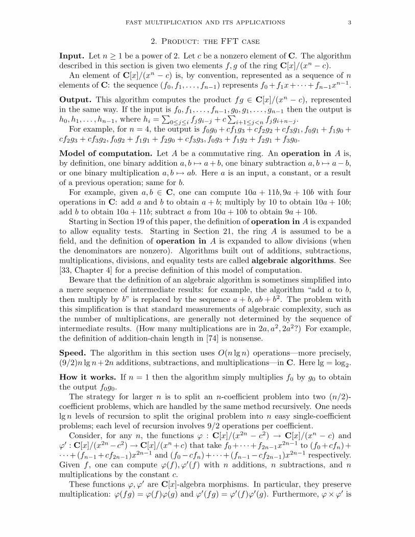
2. Product: the FFT case
Input. Let n ≥ 1 be a power of 2. Let c be a nonzero element of C. The algorithmdescribed in this section is given two elements f, g of the ring C[x]/(xn − c).
An element of C[x]/(xn − c) is, by convention, represented as a sequence of nelements of C: the sequence (f0, f1, . . . , fn−1) represents f0 +f1x+ · · ·+fn−1x
n−1.
Output. This algorithm computes the product fg ∈ C[x]/(xn − c), representedin the same way. If the input is f0, f1, . . . , fn−1, g0, g1, . . . , gn−1 then the output ish0, h1, . . . , hn−1, where hi =
∑
0≤j≤i fjgi−j + c∑
i+1≤j<n fjgi+n−j .For example, for n = 4, the output is f0g0 + cf1g3 + cf2g2 + cf3g1, f0g1 + f1g0 +
cf2g3 + cf3g2, f0g2 + f1g1 + f2g0 + cf3g3, f0g3 + f1g2 + f2g1 + f3g0.
Model of computation. Let A be a commutative ring. An operation in A is,by definition, one binary addition a, b 7→ a + b, one binary subtraction a, b 7→ a− b,or one binary multiplication a, b 7→ ab. Here a is an input, a constant, or a resultof a previous operation; same for b.
For example, given a, b ∈ C, one can compute 10a + 11b, 9a + 10b with fouroperations in C: add a and b to obtain a + b; multiply by 10 to obtain 10a + 10b;add b to obtain 10a + 11b; subtract a from 10a + 10b to obtain 9a + 10b.
Starting in Section 19 of this paper, the definition of operation in A is expandedto allow equality tests. Starting in Section 21, the ring A is assumed to be afield, and the definition of operation in A is expanded to allow divisions (whenthe denominators are nonzero). Algorithms built out of additions, subtractions,multiplications, divisions, and equality tests are called algebraic algorithms. See[33, Chapter 4] for a precise definition of this model of computation.
Beware that the definition of an algebraic algorithm is sometimes simplified intoa mere sequence of intermediate results: for example, the algorithm “add a to b,then multiply by b” is replaced by the sequence a + b, ab + b2. The problem withthis simplification is that standard measurements of algebraic complexity, such asthe number of multiplications, are generally not determined by the sequence ofintermediate results. (How many multiplications are in 2a, a2, 2a2?) For example,the definition of addition-chain length in [74] is nonsense.
Speed. The algorithm in this section uses O(n lg n) operations—more precisely,(9/2)n lg n+2n additions, subtractions, and multiplications—in C. Here lg = log2.
How it works. If n = 1 then the algorithm simply multiplies f0 by g0 to obtainthe output f0g0.
The strategy for larger n is to split an n-coefficient problem into two (n/2)-coefficient problems, which are handled by the same method recursively. One needslg n levels of recursion to split the original problem into n easy single-coefficientproblems; each level of recursion involves 9/2 operations per coefficient.
Consider, for any n, the functions ϕ : C[x]/(x2n − c2) → C[x]/(xn − c) andϕ′ : C[x]/(x2n−c2) → C[x]/(xn +c) that take f0 + · · ·+f2n−1x
2n−1 to (f0 +cfn)+· · ·+(fn−1 +cf2n−1)x
2n−1 and (f0−cfn)+ · · ·+(fn−1−cf2n−1)x2n−1 respectively.
Given f , one can compute ϕ(f), ϕ′(f) with n additions, n subtractions, and nmultiplications by the constant c.
These functions ϕ,ϕ′ are C[x]-algebra morphisms. In particular, they preservemultiplication: ϕ(fg) = ϕ(f)ϕ(g) and ϕ′(fg) = ϕ′(f)ϕ′(g). Furthermore, ϕ×ϕ′ is
4 DANIEL J. BERNSTEIN
C[x]/(x4 + 1)
x7→x
wwoooooooooooooooo
x7→x
''OOOOOOOOOOOOOOOO
C[x]/(x2 − i)
x7→√
i
������
����
���
x7→−√
i
��???
????
????
C[x]/(x2 + i)
x7→√−i
������
����
���
x7→−√−i
��???
????
????
C C C C
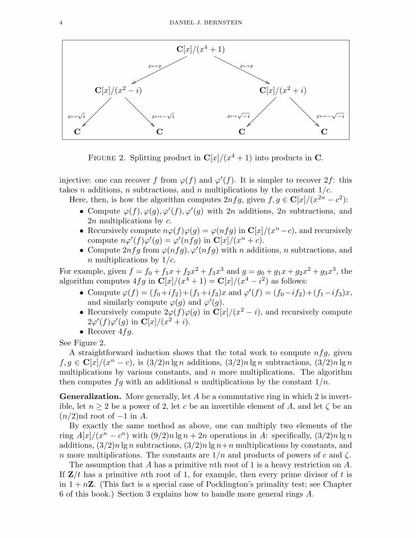
Figure 2. Splitting product in C[x]/(x4 + 1) into products in C.
injective: one can recover f from ϕ(f) and ϕ′(f). It is simpler to recover 2f : thistakes n additions, n subtractions, and n multiplications by the constant 1/c.
Here, then, is how the algorithm computes 2nfg, given f, g ∈ C[x]/(x2n − c2):
• Compute ϕ(f), ϕ(g), ϕ′(f), ϕ′(g) with 2n additions, 2n subtractions, and2n multiplications by c.
• Recursively compute nϕ(f)ϕ(g) = ϕ(nfg) in C[x]/(xn−c), and recursivelycompute nϕ′(f)ϕ′(g) = ϕ′(nfg) in C[x]/(xn + c).
• Compute 2nfg from ϕ(nfg), ϕ′(nfg) with n additions, n subtractions, andn multiplications by 1/c.
For example, given f = f0 + f1x + f2x2 + f3x
3 and g = g0 + g1x + g2x2 + g3x
3, thealgorithm computes 4fg in C[x]/(x4 + 1) = C[x]/(x4 − i2) as follows:
• Compute ϕ(f) = (f0+if2)+(f1+if3)x and ϕ′(f) = (f0−if2)+(f1−if3)x,and similarly compute ϕ(g) and ϕ′(g).
• Recursively compute 2ϕ(f)ϕ(g) in C[x]/(x2 − i), and recursively compute2ϕ′(f)ϕ′(g) in C[x]/(x2 + i).
• Recover 4fg.
See Figure 2.A straightforward induction shows that the total work to compute nfg, given
f, g ∈ C[x]/(xn − c), is (3/2)n lg n additions, (3/2)n lg n subtractions, (3/2)n lg nmultiplications by various constants, and n more multiplications. The algorithmthen computes fg with an additional n multiplications by the constant 1/n.
Generalization. More generally, let A be a commutative ring in which 2 is invert-ible, let n ≥ 2 be a power of 2, let c be an invertible element of A, and let ζ be an(n/2)nd root of −1 in A.
By exactly the same method as above, one can multiply two elements of thering A[x]/(xn − cn) with (9/2)n lg n + 2n operations in A: specifically, (3/2)n lg nadditions, (3/2)n lg n subtractions, (3/2)n lg n+n multiplications by constants, andn more multiplications. The constants are 1/n and products of powers of c and ζ.
The assumption that A has a primitive nth root of 1 is a heavy restriction on A.If Z/t has a primitive nth root of 1, for example, then every prime divisor of t isin 1 + nZ. (This fact is a special case of Pocklington’s primality test; see Chapter6 of this book.) Section 3 explains how to handle more general rings A.
FAST MULTIPLICATION AND ITS APPLICATIONS 5
Variant: radix 3. Similarly, let A be a commutative ring in which 3 is invertible,let n ≥ 3 be a power of 3, let c be an invertible element of A, and let ζ be anelement of A satisfying 1 + ζn/3 + ζ2n/3 = 0. Then one can multiply two elementsof the ring A[x]/(xn − cn) with O(n lg n) operations in A.
History. Gauss in [49, pages 265–327] was the first to point out that one canquickly compute a ring isomorphism from R[x]/(x2n−1) to R2×Cn−1 when n hasno large prime factors. In [49, pages 308–310], for example, Gauss (in completelydifferent language) mapped R[x]/(x12 − 1) to R[x]/(x3 − 1) × R[x]/(x3 + 1) ×C[x]/(x3 + i), then mapped R[x]/(x3 − 1) to R × C, mapped R[x]/(x3 + 1) toR × C, and mapped C[x]/(x3 + i) to C × C × C.
The discrete Fourier transform—this isomorphism from R[x]/(x2n − 1) toR2×Cn−1, or the analogous isomorphism from C[x]/(xn−1) to Cn—was applied tomany areas of scientific computation over the next hundred years. Gauss’s methodwas reinvented several times, as discussed in [56], and finally became widely knownafter it was reinvented and published by Cooley and Tukey in [41]. Gauss’s methodis now called the fast Fourier transform or simply the FFT.
Shortly after the Cooley-Tukey paper, Sande and Stockham pointed out thatone can quickly multiply in C[x]/(xn −1) by applying the FFT, multiplying in Cn,and applying the inverse FFT. See [108, page 229] and [50, page 573].
Fiduccia in [47] was the first to point out that each step of the FFT is an algebraisomorphism. This fact is still not widely known, despite its tremendous expositoryvalue; most expositions of the FFT use only the module structure of each step. Ihave taken Fiduccia’s idea much further in this paper and in [13], identifying thering morphisms behind all known multiplication methods.
Improvements. The algorithm explained above takes 15n lg n + 8n operations inR to multiply in C[x]/(xn − 1), if n ≥ 2 is a power of 2 and C is represented asR[i]/(i2 + 1):
• 5n lg n to transform the first input from C[x]/(xn − 1) to Cn. The FFTtakes n lg n additions and subtractions in C, totalling 2n lg n operationsin R, and (1/2)n lg n multiplications by various roots of 1 in C, totalling3n lg n operations in R.
• 5n lg n to transform the second input from C[x]/(xn − 1) to Cn.• 2n to scale one of the transforms, i.e., to multiply by the constant 1/n. One
can eliminate most of these multiplications by absorbing 1/n into otherconstants.
• 6n to multiply the two transformed inputs in Cn.• 5n lg n to transform the product from Cn back to C[x]/(xn − 1).
One can reduce each 5n lg n to 5n lg n−10n+16 for n ≥ 4 by recognizing roots of 1that allow easy multiplications: multiplications by 1 can be skipped, multiplicationsby −1 and ±i can be absorbed into subsequent computations, and multiplicationsby ±
ñi are slightly easier than general multiplications.
Gentleman and Sande in [50] pointed out another algorithm to map C[x]/(xn−1)to Cn using 5n lg n− 10n + 16 operations: map C[x]/(x2n − 1) to C[x]/(xn − 1)×C[x]/(xn + 1), twist C[x]/(xn + 1) into C[x]/(xn − 1) by mapping x → ζx, andhandle each C[x]/(xn − 1) recursively. I call this method the twisted FFT.
6 DANIEL J. BERNSTEIN
The split-radix FFT is faster: it uses only 4n lg n−6n+8 operations for n ≥ 2,so multiplication in C[x]/(xn − 1) uses only 12n lg n + O(n) operations. The split-radix FFT is a mixture of Gauss’s FFT with the Gentleman-Sande twisted FFT:it maps C[x]/(x4n − 1) to C[x]/(x2n − 1) × C[x]/(x2n + 1), maps C[x]/(x2n + 1)to C[x]/(xn − i) × C[x]/(xn + i), twists each C[x]/(xn ± i) into C[x]/(xn − 1) bymapping x → ζx, and recursively handles both C[x]/(x2n − 1) and C[x]/(xn − 1).
Another method is the real-factor FFT: map C[x]/(x4n − (2 cos 2α)x2n +1) toC[x]/(x2n − (2 cosα)xn + 1)×C[x]/(x2n + (2 cosα)xn + 1), and handle each factorrecursively. The real-factor FFT uses 4n lg n + O(n) operations if one representselements of C[x]/(x2n ± · · · ) using the basis (1, x, . . . , xn−1, x−n, x1−n, . . . , x−1).
It is difficult to assign credit for the bound 4n lg n+O(n). Yavne announced thebound 4n lg n− 6n+8 (specifically, 3n lg n− 3n+4 additions and subtractions andn lg n − 3n + 4 multiplications) in [124, page 117], and apparently had in mind amethod achieving that bound; but nobody, to my knowledge, has ever decipheredYavne’s explanation of the method. Ten years later, Bruun in [31] published thereal-factor FFT. Several years after that, Duhamel and Hollmann in [44], Martensin [83], Vetterli and Nussbaumer in [121], and Stasinski (according to [45, page263]) independently discovered the split-radix FFT.
One can multiply in R[x]/(x2n + 1) with 12n lg n + O(n) operations in R, if nis a power of 2: map R[x]/(x2n + 1) to C[x]/(xn − i), twist C[x]/(xn − i) intoC[x]/(xn − 1), and apply the split-radix FFT. This is approximately twice as fastas mapping R[x]/(x2n+1) to C[x]/(x2n+1). An alternative is to use the real-factorFFT, with R in place of C.
One can also multiply in R[x]/(x2n − 1) with 12n lg n + O(n) operations in R,if n is a power of 2: map R[x]/(x2n − 1) to R[x]/(xn − 1) ×R[x]/(xn + 1); handleR[x]/(xn−1) by the same method recursively; handle R[x]/(xn +1) as above. Thisis approximately twice as fast as mapping R[x]/(x2n − 1) to C[x]/(x2n − 1). Thisspeedup was announced by Bergland in [9], but it was already part of Gauss’s FFT.
The general strategy of all of the above algorithms is to transform f , transformg, multiply the results, and then undo the transform to recover fg. There is someredundancy here if f = g: one can easily save a factor of 1.5+o(1) by transformingf , squaring the result, and undoing the transform to recover f 2. (Of course, f2 ismuch easier to compute if 2 = 0 in A; this also saves time in Section 6.)
More generally, one can save the transform of each input, and reuse the transformin a subsequent multiplication if one knows (or observes) that the same input isshowing up again. I call this technique FFT caching. FFT caching was announcedin [42, Section 9], but it was already widely known; see, e.g., [87, Section 3.7].
Further savings are possible when one wants to compute a sum of products.Instead of undoing a transform to recover ab, undoing another transform to recovercd, and adding the results to obtain ab + cd, one can add first and then undo asingle transform to recover ab + cd. I call this technique FFT addition.
There is much more to say about FFT performance, because there are muchmore sophisticated models of computation. Real computers have operation latency,memory latency, and instruction-decoding latency, for example; a serious analysisof constant factors takes these latencies into account.
FAST MULTIPLICATION AND ITS APPLICATIONS 7
3. Product: extension
Input. Let A be a commutative ring in which 2 is invertible. Let n ≥ 1 be a powerof 2. The algorithm described in this section is given two elements f, g of the ringA[x]/(xn + 1).
An element of A[x]/(xn + 1) is, by convention, represented as a sequence of nelements of A: the sequence (f0, f1, . . . , fn−1) represents f0 +f1x+ · · ·+fn−1x
n−1.
Output. This algorithm computes the product fg ∈ A[x]/(xn + 1).
Speed. This algorithm uses O(n lg n lg lg n) operations in A: more precisely, atmost (((9/2) lg lg(n/4) + 63/2) lg(n/4) − 33/2)n operations in A if n ≥ 8.
How it works. For n ≤ 8, use the definition of multiplication in A[x]/(xn + 1).This takes at most n2 + n(n − 1) = (2n − 1)n operations in A. If n = 8 thenlg(n/4) = 1 so ((9/2) lg lg(n/4)+63/2) lg(n/4)−33/2 = 63/2−33/2 = 15 = 2n−1.
For n ≥ 16, find the unique power m of 2 such that m2 ∈ {2n, 4n}. Notice that8 ≤ m < n. Notice also that lg(n/4) − 1 ≤ 2 lg(m/4) ≤ lg(n/4), so lg lg(m/4) ≤lg lg(n/4) − 1 and 2 lg(2n/m) ≤ lg(n/4) + 3.
Define B = A[x]/(xm + 1). By induction, given f, g ∈ B, one can compute theproduct fg with at most (((9/2) lg lg(m/4)+63/2) lg(m/4)− 33/2)m operations inA. One can also compute any of the following with m operations in A: the sumf + g; the difference f − g; the product cf , where c is a constant element of A; theproduct cf , where c is a constant power of x.
There is a (2n/m)th root of −1 in B, namely xm2/2n. Therefore one can usethe algorithm explained in Section 2 to multiply quickly in B[y]/(y2n/m +1)—and,consequently, to multiply in A[x, y]/(y2n/m + 1) if each input has x-degree smallerthan m/2. This takes (9/2)(2n/m) lg(2n/m) + 2n/m easy operations in B and2n/m more multiplications in B.
Now, given f, g ∈ A[x]/(xn + 1), compute fg as follows. Consider the A[x]-algebra morphism ϕ : A[x, y]/(y2n/m + 1) → A[x]/(xn + 1) that takes y to xm/2.Find F ∈ A[x, y]/(y2n/m + 1) such that F has x-degree smaller than m/2 andϕ(F ) = f ; explicitly, F =
∑
j
∑
0≤i<m/2 fi+(m/2)jxiyj if f =
∑
fixi. Similarly
construct G from g. Compute FG as explained above. Then compute ϕ(FG) = fg;this takes n additional operations in A.
One multiplication in A[x]/(xn + 1) has thus been split into
• 2n/m multiplications in B, i.e., at most ((9 lg lg(m/4)+63) lg(m/4)−33)n ≤(((9/2) lg lg(n/4) + 27) lg(n/4) − 33)n operations in A;
• (9n/m) lg(2n/m) + 2n/m ≤ ((9/2) lg(n/4) + 31/2)n/m easy operations inB, i.e., at most ((9/2) lg(n/4) + 31/2)n operations in A; and
• n additional operations in A.
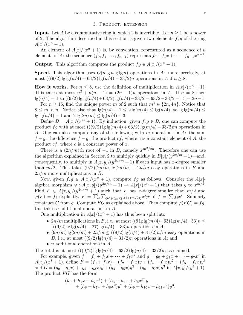
The total is at most (((9/2) lg lg(n/4) + 63/2) lg(n/4) − 33/2)n as claimed.For example, given f = f0 + f1x + · · · + f7x
7 and g = g0 + g1x + · · · + g7x7 in
A[x]/(x8 + 1), define F = (f0 + f1x) + (f2 + f3x)y + (f4 + f5x)y2 + (f6 + f7x)y3
and G = (g0 + g1x) + (g2 + g3x)y + (g4 + g5x)y2 + (g6 + g7x)y3 in A[x, y]/(y4 + 1).The product FG has the form
(h0 + h1x + h2x2) + (h3 + h4x + h5x
2)y+ (h6 + h7x + h8x
2)y2 + (h9 + h10x + h11x2)y3.
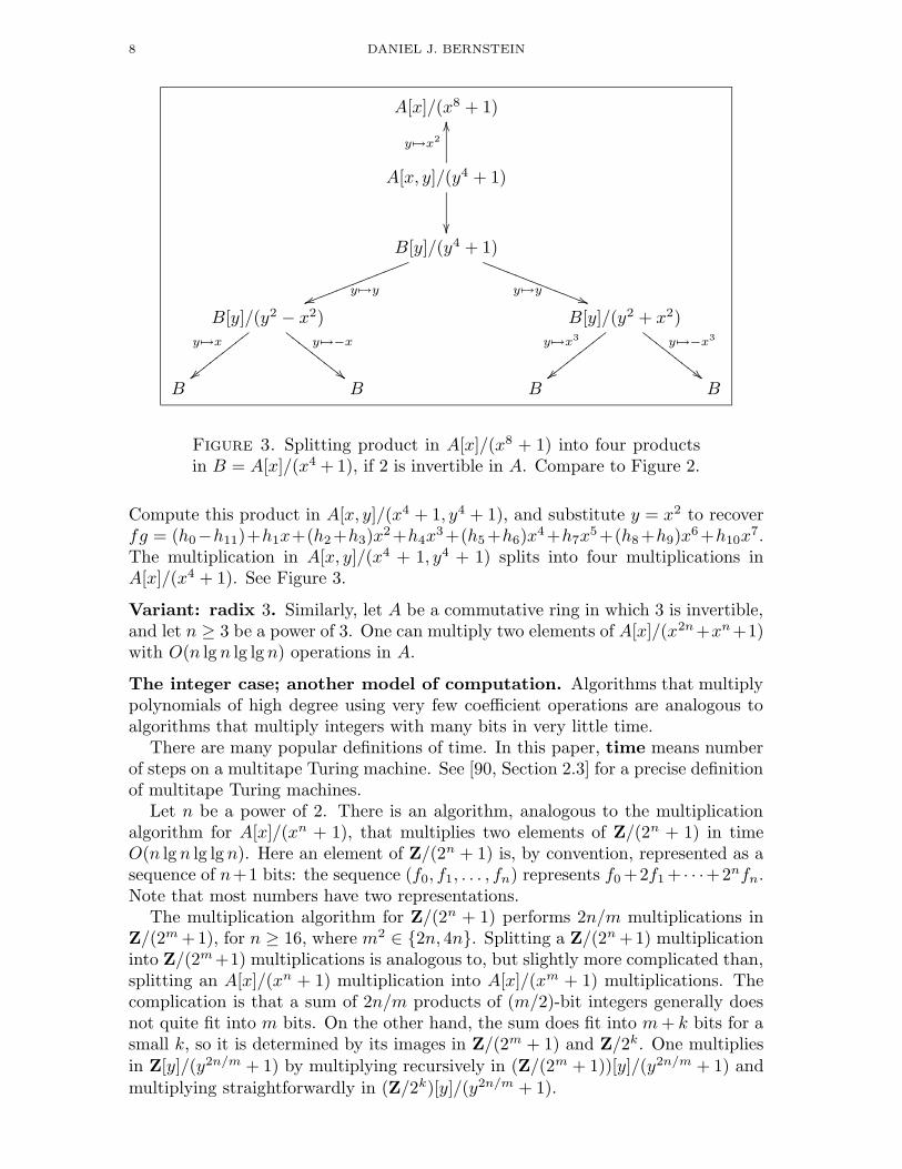
8 DANIEL J. BERNSTEIN
A[x]/(x8 + 1)
A[x, y]/(y4 + 1)
y 7→x2
OO
��B[y]/(y4 + 1)
y 7→yuulllllllllllll
y 7→y))RRRRRRRRRRRRR
B[y]/(y2 − x2)
y 7→x
||xxxx
xxxx
xy 7→−x
""FFFF
FFFF
FB[y]/(y2 + x2)
y 7→x3
||xxxx
xxxx
xy 7→−x3
""FFFF
FFFF
F
B B B B
Figure 3. Splitting product in A[x]/(x8 + 1) into four productsin B = A[x]/(x4 + 1), if 2 is invertible in A. Compare to Figure 2.
Compute this product in A[x, y]/(x4 + 1, y4 + 1), and substitute y = x2 to recoverfg = (h0−h11)+h1x+(h2+h3)x
2+h4x3+(h5+h6)x
4+h7x5+(h8+h9)x
6+h10x7.
The multiplication in A[x, y]/(x4 + 1, y4 + 1) splits into four multiplications inA[x]/(x4 + 1). See Figure 3.
Variant: radix 3. Similarly, let A be a commutative ring in which 3 is invertible,and let n ≥ 3 be a power of 3. One can multiply two elements of A[x]/(x2n +xn+1)with O(n lg n lg lg n) operations in A.
The integer case; another model of computation. Algorithms that multiplypolynomials of high degree using very few coefficient operations are analogous toalgorithms that multiply integers with many bits in very little time.
There are many popular definitions of time. In this paper, time means numberof steps on a multitape Turing machine. See [90, Section 2.3] for a precise definitionof multitape Turing machines.
Let n be a power of 2. There is an algorithm, analogous to the multiplicationalgorithm for A[x]/(xn + 1), that multiplies two elements of Z/(2n + 1) in timeO(n lg n lg lg n). Here an element of Z/(2n + 1) is, by convention, represented as asequence of n+1 bits: the sequence (f0, f1, . . . , fn) represents f0 +2f1 + · · ·+2nfn.Note that most numbers have two representations.
The multiplication algorithm for Z/(2n + 1) performs 2n/m multiplications inZ/(2m +1), for n ≥ 16, where m2 ∈ {2n, 4n}. Splitting a Z/(2n +1) multiplicationinto Z/(2m+1) multiplications is analogous to, but slightly more complicated than,splitting an A[x]/(xn + 1) multiplication into A[x]/(xm + 1) multiplications. Thecomplication is that a sum of 2n/m products of (m/2)-bit integers generally doesnot quite fit into m bits. On the other hand, the sum does fit into m + k bits for asmall k, so it is determined by its images in Z/(2m + 1) and Z/2k. One multipliesin Z[y]/(y2n/m + 1) by multiplying recursively in (Z/(2m + 1))[y]/(y2n/m + 1) andmultiplying straightforwardly in (Z/2k)[y]/(y2n/m + 1).
FAST MULTIPLICATION AND ITS APPLICATIONS 9
History. The ideas in this section were developed first in the integer case. Thecrucial point is that one can multiply in Z[y]/(ym±1) by selecting t so that Z/t hasan appropriate root of 1, mapping Z[y]/(ym±1) to (Z/t)[y]/(ym±1), and applyingan FFT over Z/t. This multiplication method was suggested by Pollard in [92],independently by Nicholson in [88, page 532], and independently by Schonhage andStrassen in [102]. Schonhage and Strassen suggested the choice t = 2m + 1 andproved the O(n lg n lg lg n) time bound.
The analogous algorithm for polynomials was mentioned by Schonhage in [98]and presented in detail by Turk in [117, Section 2]. Schonhage also suggested usingthe radix-3 FFT to multiply polynomials over fields of characteristic 2.
Nussbaumer in [89] introduced a different algorithm achieving the O(n lg n lg lg n)operation bound for polynomials. Nussbaumer’s algorithm starts in the same way,lifting (for example) A[x]/(x8 + 1) to A[x, y]/(y4 + 1) by y 7→ x2. It then mapsA[x, y]/(y4+1) to (A[y]/(y4+1))[x]/(x4−1) and applies an FFT over A[y]/(y4+1),instead of mapping A[x, y]/(y4 + 1) to (A[x]/(x4 + 1))[y]/(y4 + 1) and applying anFFT over A[x]/(x4 + 1).
Improvements. Multiplication by a constant power of x in A[x]/(xm +1) is easierthan the above analysis indicates: multiplications by 1 in A can be eliminated, andmultiplications by −1 in A can be absorbed into subsequent computations. Thetotal operation count drops from (9/2 + o(1))n lg n lg lg n to (3 + o(1))n lg n lg lg n.
The constant 3 here is the best known. There is much more to say about theo(1). See [13] for a survey of relevant techniques.
There is vastly more to say about the integer case, in part because Turing-machine time is a more complicated concept than algebraic complexity, and in partbecause real computers are more complicated than Turing machines.
10 DANIEL J. BERNSTEIN
4. Product: zero-padding and localization
Input. Let A be a commutative ring. Let n be a positive integer. The algorithmin this section is given two elements f, g of the polynomial ring A[x] such thatdeg fg < n: e.g., such that n is the total number of coefficients in f and g.
An element of A[x] is, by convention, represented as a finite sequence of elementsof A: the sequence (f0, f1, . . . , fd−1) represents f0 + f1x + · · · + fd−1x
d−1.
Output. This algorithm computes the product fg ∈ A[x].
Speed. The algorithm uses O(n lg n lg lg n) operations in A.Equivalently: The algorithm uses at most nµ(n) operations in A, where µ : N →
R is a nondecreasing positive function with µ(n) ∈ O(lg n lg lg n). The µ notationhelps simplify the run-time analysis in subsequent sections of this paper.
Special case: how it works if A = C. Given f, g ∈ C[x] such that deg fg < n,one can compute fg by using the algorithm of Section 2 to compute fg mod (xm−1)in C[x]/(xm − 1); here m is the smallest power of 2 with m ≥ n. This takesO(m lg m) = O(n lg n) operations in C.
For example, if f = f0 + f1x + f2x2 and g = g0 + g1x + g2x
2 + g3x3, use the
algorithm of Section 2 to multiply the elements f0 +f1x+f2x2 +0x3 +0x4 +0x5 +
0x6 + 0x7 and g0 + g1x + g2x2 + g3x
3 + 0x4 + 0x5 + 0x6 + 0x7 of C[x]/(x8 − 1),obtaining h0 +h1x+h2x
2 +h3x3 +h4x
4 +h5x5 +0x6 +0x7. Then fg = h0 +h1x+
h2x2 + h3x
3 + h4x4 + h5x
5. Appending zeros to an input—for example, convertingf0, f1, f2 to f0, f1, f2, 0, 0, 0, 0, 0—is called zero-padding.
In this special case A = C, the previously mentioned bound µ(n) ∈ O(lg n lg lg n)is unnecessarily pessimistic: one can take µ(n) ∈ O(lg n). Subsequent sections ofthis paper use the bound µ(n) ∈ O(lg n lg lg n), and are correspondingly pessimistic.
Similar comments apply to other rings A having appropriate roots of −1, and tonearby rings such as R.
Intermediate generality: how it works if 2 is invertible in A. Let A be anycommutative ring in which 2 is invertible. Given f, g ∈ A[x] with deg fg < n, onecan compute fg by using the algorithm of Section 3 to compute fg mod (xm + 1)in A[x]/(xm + 1); here m is the smallest power of 2 with m ≥ n. This takesO(m lg m lg lg m) = O(n lg n lg lg n) operations in A.
Intermediate generality: how it works if 3 is invertible in A. Let A be anycommutative ring in which 3 is invertible. The previous algorithm has a radix-3variant that computes fg using O(n lg n lg lg n) operations in A.
Full generality: how it works for arbitrary rings. What if neither 2 nor 3 isinvertible? Answer: Map A to the product of the localizations 2−NA and 3−NA.This map is injective; 2 is invertible in 2−NA; and 3 is invertible in 3−NA.
In other words: Given polynomials f, g over any commutative ring A, use thetechnique of Section 3 to compute 2jfg for some j; use the radix-3 variant tocompute 3kfg for some k; and then compute fg as a linear combination of 2jfgand 3kfg. This takes O(n lg n lg lg n) operations in A if deg fg < n.
Assume, for example, that deg fg < 8. Compute 16fg by computing 16fg mod(x8 − 1), and compute 9fg by computing 9fg mod (x18 + x9 + 1); then fg =4(16fg) − 7(9fg). The numbers 16 and 9 here are the denominators produced bythe algorithm of Section 3.
FAST MULTIPLICATION AND ITS APPLICATIONS 11
The integer case. An analogous algorithm computes the product of two integersin time O(n lg n lg lg n), if the output size is known to be at most n bits. (Givenf, g ∈ Z with |fg| < 2n, use the algorithm of Section 3 to compute fg mod (2m +1)in Z/(2m + 1); here m is the smallest power of 2 with m ≥ n + 1.)
Here an integer is, by convention, represented in two’s-complement notation:a sequence of bits (f0, f1, . . . , fk−1, fk) represents f0 + 2f1 + · · ·+ 2k−1fk−1 − 2kfk.
History. Karatsuba in [63] was the first to point out that integer multiplicationcan be done in subquadratic time. This result is often (e.g., in [33, page 58]) creditedto Karatsuba and Ofman, because [63] was written by Karatsuba and Ofman; but[63] explicitly credited the algorithm to Karatsuba alone.
Toom in [115] was the first to point out that integer multiplication can be donein essentially linear time: more precisely, time n exp(O(
√log n)). Schonhage in [96]
independently published the same observation a few years later. Cook in [40, page53] commented that Toom’s method could be used to quickly multiply polynomialsover finite fields.
Stockham in [108, page 230] suggested zero-padding and FFT-based multiplica-tion in C[x]/(xn − 1) as a way to multiply in C[x].
The O(n lg n lg lg n) time bound for integers is usually credited to Schonhage andStrassen; see Section 3. Cantor and Kaltofen in [37] used A → 2−NA × 3−NA toprove the O(n lg n lg lg n) operation bound for polynomials over any ring.
Improvements. The above algorithms take
• (m/n)(9/2 + o(1))n lg n operations in C to multiply in C[x]; or• (m/n)(12+ o(1))n lg n operations in R to multiply in C[x], using the split-
radix FFT or the real-factor FFT; or• (m/n)(6 + o(1))n lg n operations in R to multiply in R[x]; or• (m/n)(3 + o(1))n lg n lg lg n operations in any ring A to multiply in A[x], if
2 is invertible in A.
There are several ways to eliminate the m/n factor here. One good way is tocompute fg modulo xm + 1 for several powers m of 2 with
∑
m ≥ n, then recoverfg. For example, if n = 80000, one can recover fg from fg mod (x65536 + 1) andfg mod (x16384 + 1). A special case of this technique was pointed out by Crandalland Fagin in [42, Section 7]. See [13, Section 8] for an older technique.
One can save time at the beginning of the FFT when the input is known to bethe result of zero-padding. For example, one does not need an operation to computef0+0. Similarly, one can save time at the end of the FFT when the output is knownto have zeros: the zeros need not be recomputed.
In the context of FFT addition—for example, computing ab + cd with only fivetransforms—the transform size does not need to be large enough for ab and cd; itneed only be large enough for ab + cd. This is useful in applications where ab + cdis known to be small.
When f has a substantially larger degree than g (or vice versa), one can often savetime by splitting f into pieces of comparable size to g, and multiplying each pieceby g. Similar comments apply in Section 7. In the polynomial case, this techniqueis most often called the “overlap-add method”; it was introduced by Stockham in[108, page 230] under the name “sectioning.” The analogous technique for integersappears in [72, answer to Exercise 4.3.3–13] with credit to Schonhage.
See [13] for a survey of further techniques.
12 DANIEL J. BERNSTEIN
5. Product: completion
Input. Let A be a commutative ring. Let n be a positive integer. The algorithmin this section is given the precision-n representations of two elements f, g of thepower-series ring A[[x]].
The precision-n representation of a power series f ∈ A[[x]] is, by definition, thepolynomial f mod xn. If f =
∑
j fjxj then f mod xn = f0 + f1x + · · ·+ fn−1x
n−1.This polynomial is, in turn, represented in the usual way as its coefficient sequence(f0, f1, . . . , fn−1).
This representation does not carry complete information about f ; it is only anapproximation to f . It is nevertheless useful.
Output. This algorithm computes the precision-n representation of the productfg ∈ A[[x]]. If the input is f0, f1, . . . , fn−1, g0, g1, . . . , gn−1 then the output isf0g0, f0g1 + f1g0, f0g2 + f1g1 + f2g0, . . . , f0gn−1 + f1gn−2 + · · · + fn−1g0.
Speed. This algorithm uses O(n lg n lg lg n) operations in A: more precisely, atmost (2n − 1)µ(2n − 1) operations in A.
How it works. Given f mod xn and g mod xn, compute the polynomial product(f mod xn)(g mod xn) by the algorithm of Section 4. Throw away the coefficientsof xn, xn+1, . . . to obtain (f mod xn)(g mod xn) mod xn = fg mod xn.
For example, given the precision-3 representation f0, f1, f2 of the series f =f0 +f1x+f2x
2 + · · · , and given the precision-3 representation g0, g1, g2 of the seriesg = g0 +g1x+g2x
2 + · · · , first multiply f0 +f1x+f2x2 by g0 +g1x+g2x
2 to obtainf0g0 +(f0g1 +f1g0)x+(f0g2 +f1g1 +f2g0)x
2 +(f1g2 +f2g1)x3 +f2g2x
4; then throwaway the coefficients of x3 and x4 to obtain f0g0, f0g1 + f1g0, f0g2 + f1g1 + f2g0.
The integer case, easy completion: Q → Q2. Consider the ring Z2 of 2-adicintegers. The precision-n representation of f ∈ Z2 is, by definition, the integerf mod 2n ∈ Z. This representation of elements of Z2 as nearby elements of Z
is analogous in many ways to the representation of elements of A[[x]] as nearbyelements of A[x]. In particular, there is an analogous multiplication algorithm:given f mod 2n and g mod 2n, one can compute fg mod 2n in time O(n lg n lg lg n).
The integer case, hard completion: Q → R. Each real number f ∈ R is, byconvention, represented as a nearby element of the localization 2−NZ: an integerdivided by a power of 2. If |f | < 1, for example, then there are one or two integersd with |d| ≤ 2n such that |d/2n − f | < 1/2n.
If another real number g with |g| < 1 is similarly represented by an integer e thenfg is almost represented by the integer bde/2nc, which can be computed in timeO(n lg n lg lg n). However, the distance from fg to bde/2nc /2n may be somewhatlarger than 1/2n. This effect is called roundoff error: the output is known toslightly less precision than the input.
History. See [72, Section 4.1] for the history of positional notation.
Improvements. Operations involved in multiplying f mod xn by g mod xn canbe skipped if they are used only to compute the coefficients of xn, xn+1, . . . . Thenumber of operations skipped depends on the multiplication method; optimizingu, v 7→ uv does not necessarily optimize u, v 7→ uv mod xn. Similar comments applyto the integer case.
FAST MULTIPLICATION AND ITS APPLICATIONS 13
6. Reciprocal
Input. Let A be a commutative ring. Let n be a positive integer. The algorithmin this section is given the precision-n representation of a power series f ∈ A[[x]]with f(0) = 1.
Output. This algorithm computes the precision-n representation of the reciprocal1/f = 1+(1− f)+ (1− f)2 + · · · ∈ A[[x]]. If the input is 1, f1, f2, f3, . . . , fn−1 thenthe output is 1,−f1, f
21 − f2, 2f1f2 − f3
1 − f3, . . . , · · · − fn−1.
Speed. This algorithm uses O(n lg n lg lg n) operations in A: more precisely, atmost (8n + 2k − 8)µ(2n − 1) + (2n + 2k − 2) operations in A if n ≤ 2k.
How it works. If n = 1 then (1/f) mod xn = 1. There are 0 operations here; and(8n + 2k − 8)µ(2n − 1) + (2n + 2k − 2) = 2kµ(1) + 2k ≥ 0 since k ≥ lg n = 0.
Otherwise define m = dn/2e. Recursively compute g0 = (1/f) mod xm; notethat m < n. Then compute (1/f) mod xn as (g0 − (fg0 − 1)g0) mod xn, usingthe algorithm of Section 5 for the multiplications by g0. This works because thedifference 1/f − (g0 − (fg0 − 1)g0) is exactly f(1/f − g0)
2, which is a multiple ofx2m, hence of xn.
For example, given the precision-4 representation 1 + f1x + f2x2 + f3x
3 of f ,recursively compute g0 = (1/f) mod x2 = 1 − f1x. Multiply f by g0 modulox4 to obtain 1 + (f2 − f2
1 )x2 + (f3 − f1f2)x3. Subtract 1 and multiply by g0
modulo x4 to obtain (f2 − f21 )x2 + (f3 + f3
1 − 2f1f2)x3. Subtract from g0 to obtain
1− f1x + (f21 − f2)x
2 + (2f1f2 − f31 − f3)x
3. This is the precision-4 representationof 1/f .
The proof of speed is straightforward. By induction, the recursive computationuses at most (8m + 2(k − 1) − 8)µ(2m − 1) + (2m + 2(k − 1) − 2) operations inA, since m ≤ 2k−1. The subtraction from g0 and the subtraction of 1 use at mostn+1 operations in A. The two multiplications by g0 use at most 2(2n−1)µ(2n−1)operations in A. Apply the inequalities m ≤ (n + 1)/2 and µ(2m − 1) ≤ µ(2n − 1)to see that the total is at most (8n + 2k − 8)µ(2n − 1) + (2n + 2k − 2) as claimed.
The integer case, easy completion: Q → Q2. Let f ∈ Z2 be an odd 2-adicinteger. Then f has a reciprocal 1/f = 1 + (1 − f) + (1 − f)2 + · · · ∈ Z2.
One can compute (1/f) mod 2n, given f mod 2n, by applying the same formulaas in the power-series case: first recursively compute g0 = (1/f) mod 2dn/2e; thencompute (1/f) mod 2n as (g0+(1−fg0)g0) mod 2n. This takes time O(n lg n lg lg n).
The integer case, hard completion: Q → R. Let f ∈ R be a real number be-tween 0.25 and 1. Then f has a reciprocal g = 1 + (1 − f) + (1 − f)2 + · · · ∈ R.If g0 is a close approximation to 1/f , then g0 + (1− fg0)g0 is an approximation to1/f with nearly twice the precision. Consequently one can compute a precision-nrepresentation of 1/f , given a slightly higher-precision representation of f , in timeO(n lg n lg lg n).
The details are, thanks to roundoff error, more complicated than in the power-series case, and are not included in this paper. See [72, Algorithm 4.3.3–R] or [11,Section 8] for a complete algorithm.
14 DANIEL J. BERNSTEIN
History. Simpson in [105, page 81] presented the iteration g 7→ g − (fg − 1)g forreciprocals. Simpson also commented that one can carry out the second-to-lastiteration at about 1/2 the desired precision, the third-to-last iteration at about 1/4the desired precision, etc., so that the total time is comparable to the time for thelast iteration. I have not been able to locate earlier use of this iteration.
Simpson considered, more generally, the iteration g 7→ g − p(g)/p′(g) for rootsof a function p. The iteration g 7→ g − (fg − 1)g is the case p(g) = g−1 − f .The general case is usually called “Newton’s method,” but I see no evidence thatNewton deserves credit for it. Newton used the iteration for polynomials p, but sodid previous mathematicians. Newton’s descriptions never mentioned derivativesand were not amenable to generalization. See [77] and [125] for further discussion.
Cook in [40, pages 81–86] published details of a variable-precision reciprocalalgorithm for R taking essentially linear time, using the iteration g 7→ g− (fg−1)gwith Toom’s essentially-linear-time multiplication algorithm.
Sieveking in [104], apparently unaware of Cook’s result, published details of ananalogous reciprocal algorithm for A[[x]]. The analogy was pointed out by Kungin [80].
Improvements. Computing a reciprocal by the above algorithm takes 4 + o(1)times as many operations as computing a product. There are several ways thatthis constant 4 can be reduced. The following discussion focuses on C[[x]] andassumes that n is a power of 2. Analogous comments apply to other values of n; toA[[x]] for other rings A; to Z2; and to R.
One can achieve 3 + o(1) by skipping some multiplications by low zeros. Thepoint is that that fg0 − 1 is a multiple of xm. Write u = ((fg0 − 1) mod xn)/xm
and v = g0 mod xn−m; then u and v are polynomials of degree below n − m,and ((fg0 − 1)g0) mod xn = xmuv mod xn. One can compute uv mod xn − 1,extract the bottom n−m coefficients of the product, and insert m zeros, to obtain((fg0 − 1)g0) mod xn.
One can achieve 2 + o(1) by skipping some multiplications by high zeros andby not recomputing a stretch of known coefficients. To compute fg0 mod xn, onemultiplies f mod xn by g0 and extracts the bottom n coefficients. The point is that(f mod xn)g0 − 1 is a multiple of xm, and has degree at most m + n, so it is easilycomputed from its remainder modulo xn − 1: it has m zeros, then the top n − mcoefficients of the remainder, then the bottom n− m coefficients of the remainder.
One can achieve 5/3 + o(1) by applying FFT caching. There is a multiplicationof f mod xn by g0 modulo xn − 1, and a multiplication of (fg0 − 1) mod xn by g0
modulo xn − 1; the transform of g0 can be reused rather than recomputed.One can achieve 3/2+o(1) by evaluating a cubic rather than two quadratics. The
polynomial ((f mod xn)g0 − 1)g0 is a multiple of xm and has degree below n+ 2m,so it is easily computed from its remainders modulo xn + 1 and xm − 1. Onetransforms f mod xn, transforms g0, multiplies the first transform by the square ofthe second, subtracts the second, and untransforms the result.
Brent published 3 + o(1) in [28]. Schonhage, Grotefeld, and Vetter in [101, page256] announced 2 + o(1) without giving details. I published 28/15 + o(1) in 1998,and 3/2+ o(1) in 2000, with a rather messy algorithm; see [15]. Schonhage in [100]independently published the above 3/2 + o(1) algorithm.
FAST MULTIPLICATION AND ITS APPLICATIONS 15
7. Quotient
Input. Let A be a commutative ring. Let n be a positive integer. The algorithmin this section is given the precision-n representations of power series f, h ∈ A[[x]]such that f(0) = 1.
Output. This algorithm computes the precision-n representation of h/f ∈ A[[x]].If the input is 1, f1, f2, . . . , fn−1, h0, h1, h2, . . . , hn−1 then the output is
h0,h1 − f1h0,h2 − f1h1 + (f2
1 − f2)h0,...hn−1 − · · · + (· · · − fn−1)h0.
Speed. This algorithm uses O(n lg n lg lg n) operations in A: more precisely, atmost (10n + 2k − 9)µ(2n − 1) + (2n + 2k − 2) operations in A if n ≤ 2k.
How it works. First compute a precision-n approximation to 1/f as explained inSection 6. Then multiply by h as explained in Section 5.
The integer case, easy completion: Q → Q2. Let h and f be elements of Z2
with f odd. Given f mod 2n and h mod 2n, one can compute (h/f) mod 2n in timeO(n lg n lg lg n) by the same method.
The integer case, hard completion: Q → R. Let h and f be elements of R
with 0.5 ≤ f ≤ 1. One can compute a precision-n representation of h/f , givenslightly higher-precision representations of f and h, in time O(n lg n lg lg n). Asusual, roundoff error complicates the algorithm.
Improvements. One can improve the number of operations for a reciprocal to3/2 + o(1) times the number of operations for a product, as discussed in Section 6,so one can improve the number of operations for a quotient to 5/2+ o(1) times thenumber of operations for a product.
The reader may be wondering at this point why quotient deserves to be discussedseparately from reciprocal. Answer: Further improvements are possible. Karp andMarkstein in [66] pointed out that a quotient computation could profitably avoidsome of the work in a reciprocal computation. I achieved a gap of 13/15 + o(1) in1998 and 2/3 + o(1) in 2000, combining the Karp-Markstein idea with some FFTreuse; see [15]. In 2004, Hanrot and Zimmermann announced a gap of 7/12 + o(1):i.e., the number of operations for a quotient is 25/12 + o(1) times the number ofoperations for a product.
16 DANIEL J. BERNSTEIN
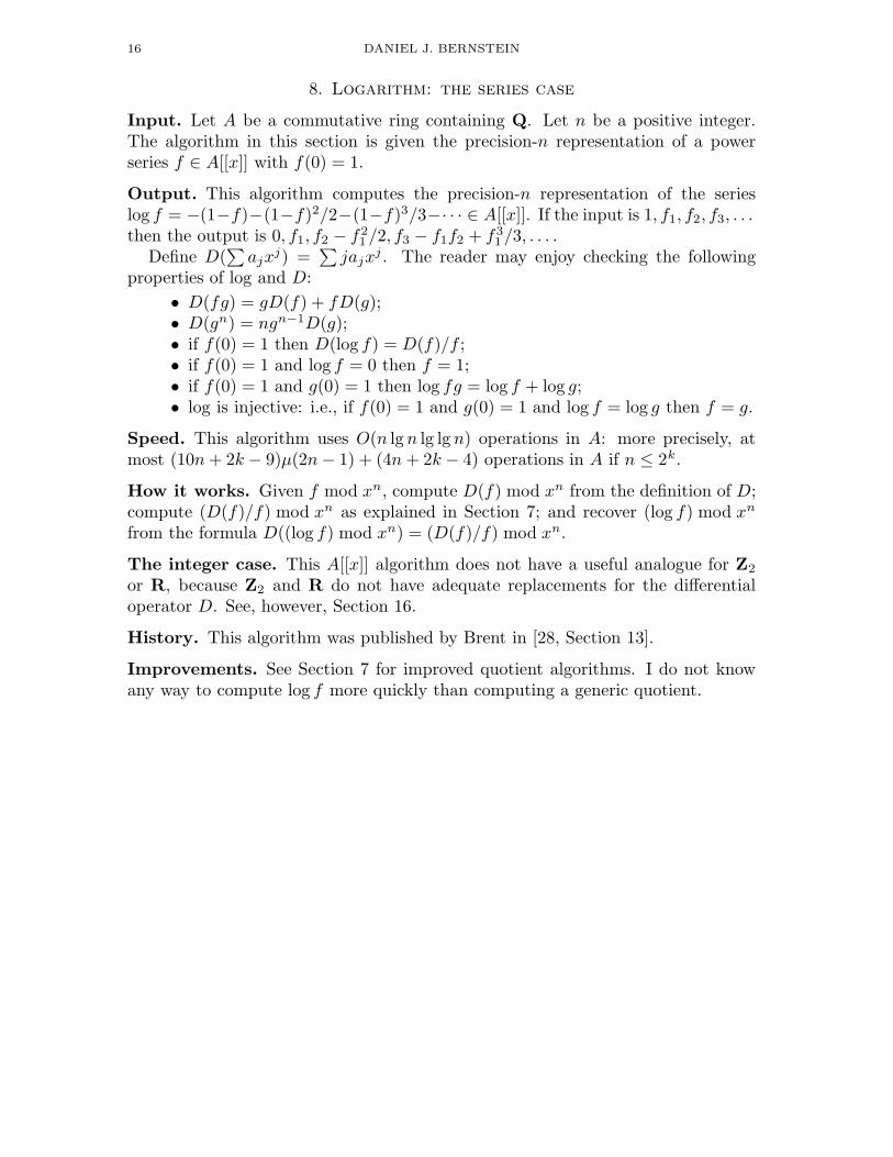
8. Logarithm: the series case
Input. Let A be a commutative ring containing Q. Let n be a positive integer.The algorithm in this section is given the precision-n representation of a powerseries f ∈ A[[x]] with f(0) = 1.
Output. This algorithm computes the precision-n representation of the serieslog f = −(1−f)−(1−f)2/2−(1−f)3/3−· · · ∈ A[[x]]. If the input is 1, f1, f2, f3, . . .then the output is 0, f1, f2 − f2
1 /2, f3 − f1f2 + f31 /3, . . . .
Define D(∑
ajxj) =
∑
jajxj . The reader may enjoy checking the following
properties of log and D:
• D(fg) = gD(f) + fD(g);• D(gn) = ngn−1D(g);• if f(0) = 1 then D(log f) = D(f)/f ;• if f(0) = 1 and log f = 0 then f = 1;• if f(0) = 1 and g(0) = 1 then log fg = log f + log g;• log is injective: i.e., if f(0) = 1 and g(0) = 1 and log f = log g then f = g.
Speed. This algorithm uses O(n lg n lg lg n) operations in A: more precisely, atmost (10n + 2k − 9)µ(2n − 1) + (4n + 2k − 4) operations in A if n ≤ 2k.
How it works. Given f mod xn, compute D(f) mod xn from the definition of D;compute (D(f)/f) mod xn as explained in Section 7; and recover (log f) mod xn
from the formula D((log f) mod xn) = (D(f)/f) mod xn.
The integer case. This A[[x]] algorithm does not have a useful analogue for Z2
or R, because Z2 and R do not have adequate replacements for the differentialoperator D. See, however, Section 16.
History. This algorithm was published by Brent in [28, Section 13].
Improvements. See Section 7 for improved quotient algorithms. I do not knowany way to compute log f more quickly than computing a generic quotient.
FAST MULTIPLICATION AND ITS APPLICATIONS 17
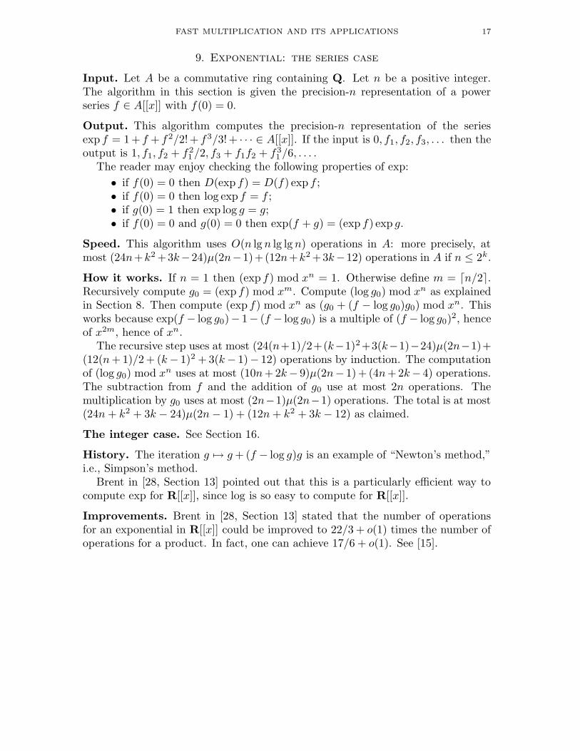
9. Exponential: the series case
Input. Let A be a commutative ring containing Q. Let n be a positive integer.The algorithm in this section is given the precision-n representation of a powerseries f ∈ A[[x]] with f(0) = 0.
Output. This algorithm computes the precision-n representation of the seriesexp f = 1+ f + f2/2!+ f3/3!+ · · · ∈ A[[x]]. If the input is 0, f1, f2, f3, . . . then theoutput is 1, f1, f2 + f2
1 /2, f3 + f1f2 + f31 /6, . . . .
The reader may enjoy checking the following properties of exp:
• if f(0) = 0 then D(exp f) = D(f) exp f ;• if f(0) = 0 then log exp f = f ;• if g(0) = 1 then exp log g = g;• if f(0) = 0 and g(0) = 0 then exp(f + g) = (exp f) exp g.
Speed. This algorithm uses O(n lg n lg lg n) operations in A: more precisely, atmost (24n+k2 +3k−24)µ(2n−1)+(12n+k2 +3k−12) operations in A if n ≤ 2k.
How it works. If n = 1 then (exp f) mod xn = 1. Otherwise define m = dn/2e.Recursively compute g0 = (exp f) mod xm. Compute (log g0) mod xn as explainedin Section 8. Then compute (exp f) mod xn as (g0 + (f − log g0)g0) mod xn. Thisworks because exp(f − log g0)− 1− (f − log g0) is a multiple of (f − log g0)
2, henceof x2m, hence of xn.
The recursive step uses at most (24(n+1)/2+(k−1)2+3(k−1)−24)µ(2n−1)+(12(n + 1)/2 + (k − 1)2 + 3(k − 1)− 12) operations by induction. The computationof (log g0) mod xn uses at most (10n+2k− 9)µ(2n− 1)+ (4n+2k− 4) operations.The subtraction from f and the addition of g0 use at most 2n operations. Themultiplication by g0 uses at most (2n−1)µ(2n−1) operations. The total is at most(24n + k2 + 3k − 24)µ(2n − 1) + (12n + k2 + 3k − 12) as claimed.
The integer case. See Section 16.
History. The iteration g 7→ g + (f − log g)g is an example of “Newton’s method,”i.e., Simpson’s method.
Brent in [28, Section 13] pointed out that this is a particularly efficient way tocompute exp for R[[x]], since log is so easy to compute for R[[x]].
Improvements. Brent in [28, Section 13] stated that the number of operationsfor an exponential in R[[x]] could be improved to 22/3 + o(1) times the number ofoperations for a product. In fact, one can achieve 17/6 + o(1). See [15].
18 DANIEL J. BERNSTEIN
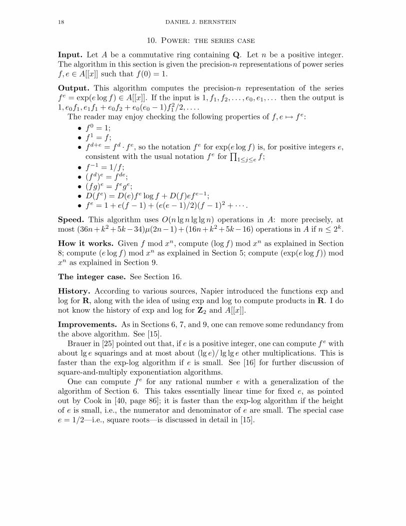
10. Power: the series case
Input. Let A be a commutative ring containing Q. Let n be a positive integer.The algorithm in this section is given the precision-n representations of power seriesf, e ∈ A[[x]] such that f(0) = 1.
Output. This algorithm computes the precision-n representation of the seriesfe = exp(e log f) ∈ A[[x]]. If the input is 1, f1, f2, . . . , e0, e1, . . . then the output is1, e0f1, e1f1 + e0f2 + e0(e0 − 1)f2
1 /2, . . . .The reader may enjoy checking the following properties of f, e 7→ f e:
• f0 = 1;• f1 = f ;• fd+e = fd · fe, so the notation fe for exp(e log f) is, for positive integers e,
consistent with the usual notation f e for∏
1≤j≤e f ;
• f−1 = 1/f ;• (fd)e = fde;• (fg)e = fege;• D(fe) = D(e)fe log f + D(f)efe−1;• fe = 1 + e(f − 1) + (e(e − 1)/2)(f − 1)2 + · · · .
Speed. This algorithm uses O(n lg n lg lg n) operations in A: more precisely, atmost (36n+k2 +5k−34)µ(2n−1)+(16n+k2 +5k−16) operations in A if n ≤ 2k.
How it works. Given f mod xn, compute (log f) mod xn as explained in Section8; compute (e log f) mod xn as explained in Section 5; compute (exp(e log f)) modxn as explained in Section 9.
The integer case. See Section 16.
History. According to various sources, Napier introduced the functions exp andlog for R, along with the idea of using exp and log to compute products in R. I donot know the history of exp and log for Z2 and A[[x]].
Improvements. As in Sections 6, 7, and 9, one can remove some redundancy fromthe above algorithm. See [15].
Brauer in [25] pointed out that, if e is a positive integer, one can compute f e withabout lg e squarings and at most about (lg e)/ lg lg e other multiplications. This isfaster than the exp-log algorithm if e is small. See [16] for further discussion ofsquare-and-multiply exponentiation algorithms.
One can compute fe for any rational number e with a generalization of thealgorithm of Section 6. This takes essentially linear time for fixed e, as pointedout by Cook in [40, page 86]; it is faster than the exp-log algorithm if the heightof e is small, i.e., the numerator and denominator of e are small. The special casee = 1/2—i.e., square roots—is discussed in detail in [15].
FAST MULTIPLICATION AND ITS APPLICATIONS 19
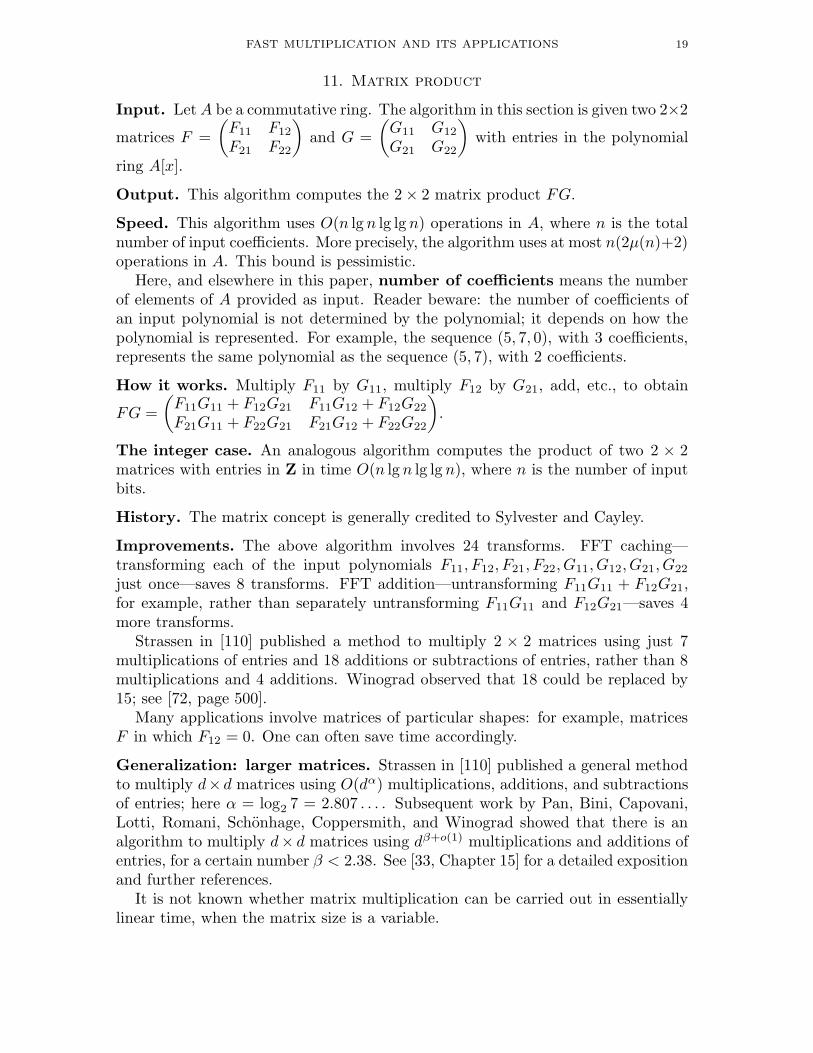
11. Matrix product
Input. Let A be a commutative ring. The algorithm in this section is given two 2×2
matrices F =
(
F11 F12
F21 F22
)
and G =
(
G11 G12
G21 G22
)
with entries in the polynomial
ring A[x].
Output. This algorithm computes the 2 × 2 matrix product FG.
Speed. This algorithm uses O(n lg n lg lg n) operations in A, where n is the totalnumber of input coefficients. More precisely, the algorithm uses at most n(2µ(n)+2)operations in A. This bound is pessimistic.
Here, and elsewhere in this paper, number of coefficients means the numberof elements of A provided as input. Reader beware: the number of coefficients ofan input polynomial is not determined by the polynomial; it depends on how thepolynomial is represented. For example, the sequence (5, 7, 0), with 3 coefficients,represents the same polynomial as the sequence (5, 7), with 2 coefficients.
How it works. Multiply F11 by G11, multiply F12 by G21, add, etc., to obtain
FG =
(
F11G11 + F12G21 F11G12 + F12G22
F21G11 + F22G21 F21G12 + F22G22
)
.
The integer case. An analogous algorithm computes the product of two 2 × 2matrices with entries in Z in time O(n lg n lg lg n), where n is the number of inputbits.
History. The matrix concept is generally credited to Sylvester and Cayley.
Improvements. The above algorithm involves 24 transforms. FFT caching—transforming each of the input polynomials F11, F12, F21, F22, G11, G12, G21, G22
just once—saves 8 transforms. FFT addition—untransforming F11G11 + F12G21,for example, rather than separately untransforming F11G11 and F12G21—saves 4more transforms.
Strassen in [110] published a method to multiply 2 × 2 matrices using just 7multiplications of entries and 18 additions or subtractions of entries, rather than 8multiplications and 4 additions. Winograd observed that 18 could be replaced by15; see [72, page 500].
Many applications involve matrices of particular shapes: for example, matricesF in which F12 = 0. One can often save time accordingly.
Generalization: larger matrices. Strassen in [110] published a general methodto multiply d×d matrices using O(dα) multiplications, additions, and subtractionsof entries; here α = log2 7 = 2.807 . . . . Subsequent work by Pan, Bini, Capovani,Lotti, Romani, Schonhage, Coppersmith, and Winograd showed that there is analgorithm to multiply d× d matrices using dβ+o(1) multiplications and additions ofentries, for a certain number β < 2.38. See [33, Chapter 15] for a detailed expositionand further references.
It is not known whether matrix multiplication can be carried out in essentiallylinear time, when the matrix size is a variable.
20 DANIEL J. BERNSTEIN
12. Product tree
Input. Let A be a commutative ring. Let t be a nonnegative integer. The algo-rithm in this section is given 2 × 2 matrices M1,M2, . . . ,Mt with entries in A[x].
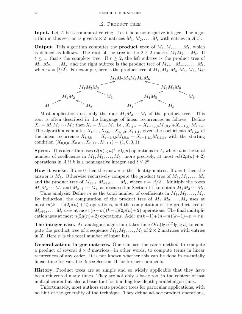
Output. This algorithm computes the product tree of M1,M2, . . . ,Mt, whichis defined as follows. The root of the tree is the 2 × 2 matrix M1M2 · · ·Mt. Ift ≤ 1, that’s the complete tree. If t ≥ 2, the left subtree is the product tree ofM1,M2, . . . ,Ms, and the right subtree is the product tree of Ms+1,Ms+2, . . . ,Mt,where s = dt/2e. For example, here is the product tree of M1,M2,M3,M4,M5,M6:
M1M2M3M4M5M6
M1M2M3
33fffffffM4M5M6
kkXXXXXXX
M1M2
66mmm
M3
hhQQQQM4M5
66mmm
M6
hhQQQQ
M1
66mmmmM2
hhQQQQM4
66mmmmM5
hhQQQQ
Most applications use only the root M1M2 · · ·Mt of the product tree. Thisroot is often described in the language of linear recurrences as follows. DefineXi = M1M2 · · ·Mi; then Xi = Xi−1Mi, i.e., Xi,j,k = Xi−1,j,0Mi,0,k+Xi−1,j,1Mi,1,k.The algorithm computes Xt,0,0, Xt,0,1, Xt,1,0, Xt,1,1, given the coefficients Mi,j,k ofthe linear recurrence Xi,j,k = Xi−1,j,0Mi,0,k + Xi−1,j,1Mi,1,k, with the startingcondition (X0,0,0, X0,0,1, X0,1,0, X0,1,1) = (1, 0, 0, 1).
Speed. This algorithm uses O(n(lg n)2 lg lg n) operations in A, where n is the totalnumber of coefficients in M1,M2, . . . ,Mt: more precisely, at most nk(2µ(n) + 2)operations in A if k is a nonnegative integer and t ≤ 2k.
How it works. If t = 0 then the answer is the identity matrix. If t = 1 then theanswer is M1. Otherwise recursively compute the product tree of M1,M2, . . . ,Ms
and the product tree of Ms+1,Ms+2, . . . ,Mt, where s = dt/2e. Multiply the rootsM1M2 · · ·Ms and Ms+1 · · ·Mt, as discussed in Section 11, to obtain M1M2 · · ·Mt.
Time analysis: Define m as the total number of coefficients in M1,M2, . . . ,Ms.By induction, the computation of the product tree of M1,M2, . . . ,Ms uses atmost m(k − 1)(2µ(n) + 2) operations, and the computation of the product tree ofMs+1, . . . ,Mt uses at most (n−m)(k−1)(2µ(n)+2) operations. The final multipli-cation uses at most n(2µ(n)+2) operations. Add: m(k−1)+(n−m)(k−1)+n = nk.
The integer case. An analogous algorithm takes time O(n(lg n)2 lg lg n) to com-pute the product tree of a sequence M1,M2, . . . ,Mt of 2 × 2 matrices with entriesin Z. Here n is the total number of input bits.
Generalization: larger matrices. One can use the same method to computea product of several d × d matrices—in other words, to compute terms in linearrecurrences of any order. It is not known whether this can be done in essentiallylinear time for variable d; see Section 11 for further comments.
History. Product trees are so simple and so widely applicable that they havebeen reinvented many times. They are not only a basic tool in the context of fastmultiplication but also a basic tool for building low-depth parallel algorithms.
Unfortunately, most authors state product trees for particular applications, withno hint of the generality of the technique. They define ad-hoc product operations,
FAST MULTIPLICATION AND ITS APPLICATIONS 21
and prove associativity of their product operations from scratch, never realizingthat these operations are special cases of matrix product.
Weinberger and Smith in [123] published the “carry-lookahead adder,” a low-depth parallel circuit for computing the sum of two nonnegative integers, with theinputs and output represented in the usual way as bit strings. The Weinberger-Smith algorithm computes (in different language) a product(
a1 0b1 1
)(
a2 0b2 1
)
· · ·(
at 0bt 1
)
=
(
a1a2 · · · at 0bt + bt−1at + bt−2at−1at + · · · + b1a2 · · · at 1
)
of matrices over the Boole algebra {0, 1} by multiplying pairs of matrices in parallel,then multiplying pairs of pairs in parallel, and so on for approximately lg t steps.
Estrin in [46] published a low-depth parallel algorithm for evaluating a one-variable polynomial. Estrin’s algorithm computes (in different language) a product
(
a 0b1 1
)(
a 0b2 1
)
· · ·(
a 0bt 1
)
=
(
at 0bt + bt−1a + bt−2a
2 + · · · + b1at−1 1
)
by multiplying pairs, pairs of pairs, etc.Schonhage, as reported in [69, Exercise 4.4–13], pointed out that one can convert
integers from base 10 to base 2 in essentially linear time. Schonhage’s algorithmcomputes (in different language) a product
(
10 0b1 1
)(
10 0b2 1
)
· · ·(
10 0bt 1
)
=
(
10t 0bt + 10bt−1 + 100bt−2 + · · · + 10t−1b1 1
)
by multiplying pairs of matrices, then pairs of pairs, etc.Knuth in [70, Theorem 1] published an algorithm to convert a continued fraction
to a fraction in essentially linear time. Knuth’s algorithm is (in different language)another example of the product-tree algorithm; see Section 14 for details.
Moenck and Borodin in [85, page 91] and [20, page 372] pointed out that one cancompute the product tree—and thus the product—of a sequence of polynomials ora sequence of integers in essentially linear time. Beware that the Moenck-Borodin“theorems” assume that all of the inputs are “single precision”; it is unclear whatthis is supposed to mean for integers.
Moenck and Borodin also pointed out an algorithm to add fractions in essentiallylinear time. This algorithm is (in different language) yet another example of theproduct-tree algorithm. See Section 13 for details and further historical notes.
Meanwhile, in the context of parallel algorithms, Stone and Kogge published theproduct-tree algorithm in a reasonable level of generality in [109], [76], and [75], withpolynomial evaluation and continued-fraction-to-fraction conversion (“tridiagonal-linear-system solution”) as examples. Stone commented that linear recurrences ofany order could be phrased as matrix products—see [109, page 34] and [109, page37]—but, unfortunately, made little use of matrices elsewhere in his presentation.
Kogge and Stone in [76, page 792] credited Robert Downs, Harvard Lomax, andH. R. G. Trout for independent discoveries of general product-tree algorithms. Theyalso stated that special cases of the algorithm were “known to J. J. Sylvester asearly as 1853”; but I see no evidence that Sylvester ever formed a product tree inthat context or any other context. Sylvester in [114] (cited in [70] and [109]) simplypointed out the associativity of continued fractions.
Brent in [26, Section 6] pointed out that the numerator and denominator of1 + 1/2 + 1/3! + · · · + 1/t! ≈ exp 1 could be computed quickly. Brent’s algorithm
22 DANIEL J. BERNSTEIN
formed (in different language) a product tree for(
1 01 1
)(
2 01 1
)
· · ·(
t 01 1
)
=
(
t! 0t! + t!/2 + · · · + t(t − 1) + t + 1 1
)
.
Brent also addressed exp for more general inputs, as discussed in Section 15; and π,via arctan. Brent described his method as a mixed-radix adaptation of Schonhage’sbase-conversion algorithm. Evidently he had in mind the product
(
a1 0b1 c
)(
a2 0b2 c
)
· · ·(
at 0bt c
)
=
(
a1a2 · · · at 0ct−1bt + ct−2bt−1at + · · · + b1a2 · · · at ct
)
corresponding to the sum∑
1≤k≤t ck−1bk/a1 · · · ak. Brent and McMillan mentioned
in [30, page 308] that the sum∑
1≤k≤t nk(−1)k−1/k!k could be handled similarly.
I gave a reasonably general statement of the product-tree algorithm in [10], witha few series and continued fractions as examples. I pointed out that computingM1M2 · · ·Mt takes time O(t(lg t)3 lg lg t) in the common case that the entries ofMj are bounded by polynomials in j.
Gosper presented a wide range of illustrative examples of matrix products in[51], emphasizing their “notational, analytic, and computational virtues.” Gosperbriefly stated the product-tree algorithm in [51, page 263], and credited it to RichSchroeppel.
Chudnovsky and Chudnovsky in [38, pages 115–118] stated the product-treealgorithm for matrices Mj whose entries depend rationally on j. They gave abroad class of series as examples in [38, pages 123–134]. They called the algorithm“a well-known method to accelerate the (numerical) solution of linear recurrences.”
Karatsuba used product trees (in different language) to evaluate various sumsin several papers starting in 1991 and culminating in [64].
See [53], [118], [22, Section 7], and [119] for further uses of product trees toevaluate sums.
Improvements. One can change s in the definition of a product tree and in theproduct-tree algorithm. The choice s = dt/2e, balancing s against t − s, is notnecessarily the fastest way to compute M1M2 · · ·Mt: when M1,M2, . . . ,Mt havewidely varying degrees, it is much better to balance deg M1 +deg M2 + · · ·+deg Ms
against deg Ms+1 +deg Ms+2 + · · ·+deg Mt. Strassen proved in [113, Theorem 3.2]that a slightly more complicated strategy is within a constant factor of optimal.
In some applications, M1,M2, . . . ,Mt are known to commute. One can oftenpermute M1,M2, . . . ,Mt for slightly higher speed. Strassen in [113, Theorem 2.2]pointed out a particularly fast, and pleasantly simple, algorithm: find the twomatrices of smallest degree, replace them by their product, and repeat. See [33,Section 2.3] for an exposition.
Robert Kramer has recently pointed out another product-tree speedup. Suppose,as an illustration, that M1,M2,M3,M4 each have degree close to n. To multiplyM1 by M2, one applies a size-2n transform to each of M1 and M2, multipliesthe transforms, and untransforms the result. To multiply M1M2 by M3M4, onestarts by applying a size-4n transform to M1M2. Kramer’s idea, which I call FFT
doubling, is that the first half of the size-4n transform of M1M2 is exactly thesize-2n transform of M1M2, which is already known. This idea saves two halves ofevery three transforms in a large balanced product-tree computation.
FAST MULTIPLICATION AND ITS APPLICATIONS 23
13. Sum of fractions
Input. Let A be a commutative ring. Let t be a positive integer. The algorithmin this section is given 2t polynomials f1, g1, f2, g2, . . . , ft, gt ∈ A[x].
Output. This algorithm computes h = f1g2 · · · gt + g1f2 · · · gt + · · · + g1g2 · · · ft,along with g1g2 · · · gt.
The reader may think of this output as follows: the algorithm computes the sumh/g1g2 · · · gt of the fractions f1/g1, f2/g2, . . . , ft/gt. The equation h/g1g2 · · · gt =f1/g1+f2/g2+· · ·+ft/gt holds in any A[x]-algebra where g1, g2, . . . , gt are invertible:
in particular, in the localization g−N
1 g−N
2 . . . g−N
t A[x].
Speed. This algorithm uses O(n(lg n)2 lg lg n) operations in A, where n is the totalnumber of coefficients in the input polynomials.
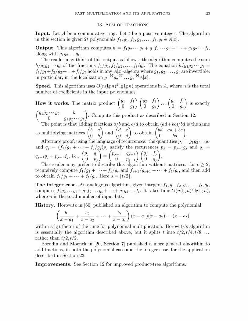
How it works. The matrix product
(
g1 f1
0 g1
)(
g2 f2
0 g2
)
. . .
(
gt ft
0 gt
)
is exactly(
g1g2 · · · gt h0 g1g2 · · · gt
)
. Compute this product as described in Section 12.
The point is that adding fractions a/b and c/d to obtain (ad+bc)/bd is the same
as multiplying matrices
(
b a0 b
)
and
(
d c0 d
)
to obtain
(
bd ad + bc0 bd
)
.
Alternate proof, using the language of recurrences: the quantities pj = g1g2 · · · gj
and qj = (f1/g1 + · · · + fj/gj)pj satisfy the recurrences pj = pj−1gj and qj =
qj−1gj + pj−1fj , i.e.,
(
pj qj
0 pj
)
=
(
pj−1 qj−1
0 pj−1
)(
gj fj
0 gj
)
.
The reader may prefer to describe this algorithm without matrices: for t ≥ 2,recursively compute f1/g1 + · · · + fs/gs and fs+1/gs+1 + · · · + ft/gt, and then addto obtain f1/g1 + · · · + ft/gt. Here s = dt/2e.The integer case. An analogous algorithm, given integers f1, g1, f2, g2, . . . , ft, gt,computes f1g2 . . . gt + g1f2 . . . gt + · · ·+ g1g2 . . . ft. It takes time O(n(lg n)2 lg lg n),where n is the total number of input bits.
History. Horowitz in [60] published an algorithm to compute the polynomial(
b1
x − a1+
b2
x − a2+ · · · + bt
x − at
)
(x − a1)(x − a2) · · · (x − at)
within a lg t factor of the time for polynomial multiplication. Horowitz’s algorithmis essentially the algorithm described above, but it splits t into t/2, t/4, t/8, . . .rather than t/2, t/2.
Borodin and Moenck in [20, Section 7] published a more general algorithm toadd fractions, in both the polynomial case and the integer case, for the applicationdescribed in Section 23.
Improvements. See Section 12 for improved product-tree algorithms.
24 DANIEL J. BERNSTEIN
14. Fraction from continued fraction
Input. Let A be a commutative ring. Let t be a nonnegative integer. The algo-rithm in this section is given t polynomials q1, q2, . . . , qt ∈ A[x] such that, for eachi, at least one of qi, qi+1 is nonzero.
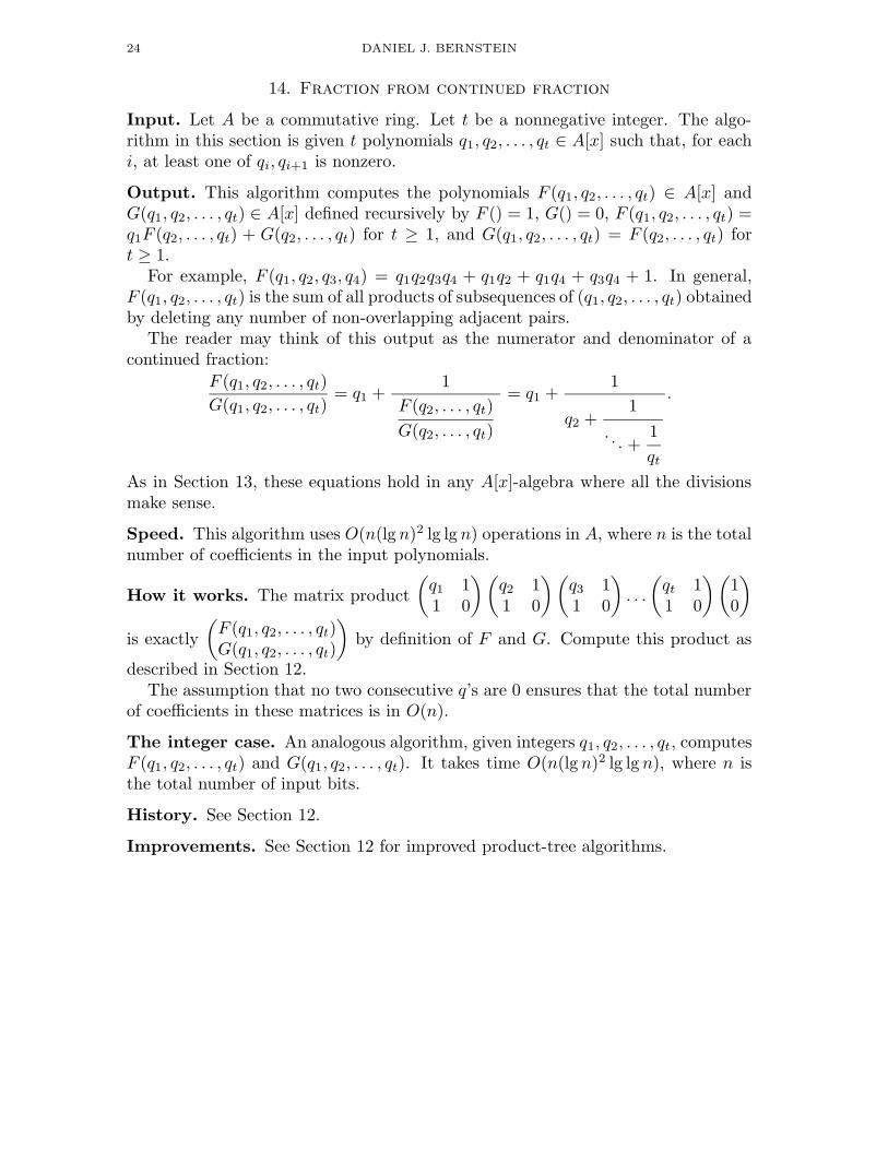
Output. This algorithm computes the polynomials F (q1, q2, . . . , qt) ∈ A[x] andG(q1, q2, . . . , qt) ∈ A[x] defined recursively by F () = 1, G() = 0, F (q1, q2, . . . , qt) =q1F (q2, . . . , qt) + G(q2, . . . , qt) for t ≥ 1, and G(q1, q2, . . . , qt) = F (q2, . . . , qt) fort ≥ 1.
For example, F (q1, q2, q3, q4) = q1q2q3q4 + q1q2 + q1q4 + q3q4 + 1. In general,F (q1, q2, . . . , qt) is the sum of all products of subsequences of (q1, q2, . . . , qt) obtainedby deleting any number of non-overlapping adjacent pairs.
The reader may think of this output as the numerator and denominator of acontinued fraction:
F (q1, q2, . . . , qt)
G(q1, q2, . . . , qt)= q1 +
1
F (q2, . . . , qt)
G(q2, . . . , qt)
= q1 +1
q2 +1
. . . +1
qt
.
As in Section 13, these equations hold in any A[x]-algebra where all the divisionsmake sense.
Speed. This algorithm uses O(n(lg n)2 lg lg n) operations in A, where n is the totalnumber of coefficients in the input polynomials.
How it works. The matrix product
(
q1 11 0
)(
q2 11 0
)(
q3 11 0
)
. . .
(
qt 11 0
)(
10
)
is exactly
(
F (q1, q2, . . . , qt)G(q1, q2, . . . , qt)
)
by definition of F and G. Compute this product as
described in Section 12.The assumption that no two consecutive q’s are 0 ensures that the total number
of coefficients in these matrices is in O(n).
The integer case. An analogous algorithm, given integers q1, q2, . . . , qt, computesF (q1, q2, . . . , qt) and G(q1, q2, . . . , qt). It takes time O(n(lg n)2 lg lg n), where n isthe total number of input bits.
History. See Section 12.
Improvements. See Section 12 for improved product-tree algorithms.
FAST MULTIPLICATION AND ITS APPLICATIONS 25
15. Exponential: the short case
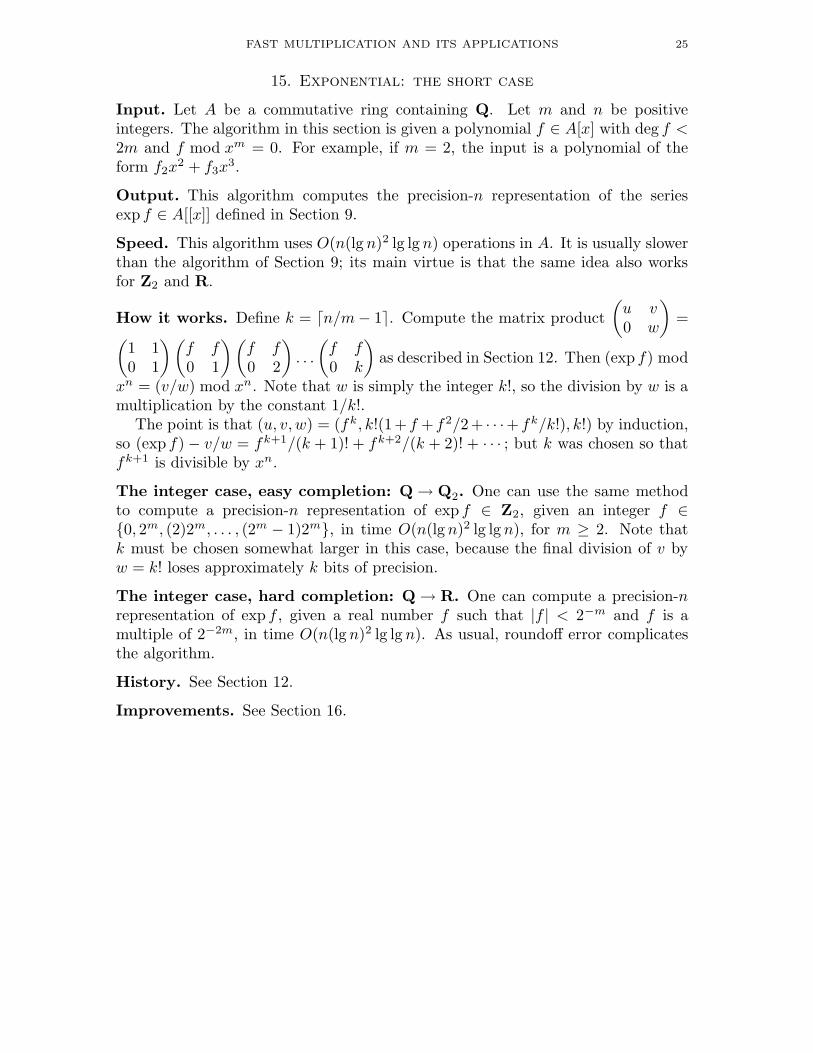
Input. Let A be a commutative ring containing Q. Let m and n be positiveintegers. The algorithm in this section is given a polynomial f ∈ A[x] with deg f <2m and f mod xm = 0. For example, if m = 2, the input is a polynomial of theform f2x
2 + f3x3.
Output. This algorithm computes the precision-n representation of the seriesexp f ∈ A[[x]] defined in Section 9.
Speed. This algorithm uses O(n(lg n)2 lg lg n) operations in A. It is usually slowerthan the algorithm of Section 9; its main virtue is that the same idea also worksfor Z2 and R.
How it works. Define k = dn/m − 1e. Compute the matrix product
(
u v0 w
)
=(
1 10 1
)(
f f0 1
)(
f f0 2
)
. . .
(
f f0 k
)
as described in Section 12. Then (exp f) mod
xn = (v/w) mod xn. Note that w is simply the integer k!, so the division by w is amultiplication by the constant 1/k!.
The point is that (u, v, w) = (fk, k!(1+ f + f2/2+ · · ·+ fk/k!), k!) by induction,so (exp f) − v/w = fk+1/(k + 1)! + fk+2/(k + 2)! + · · · ; but k was chosen so thatfk+1 is divisible by xn.
The integer case, easy completion: Q → Q2. One can use the same methodto compute a precision-n representation of exp f ∈ Z2, given an integer f ∈{0, 2m, (2)2m, . . . , (2m − 1)2m}, in time O(n(lg n)2 lg lg n), for m ≥ 2. Note thatk must be chosen somewhat larger in this case, because the final division of v byw = k! loses approximately k bits of precision.
The integer case, hard completion: Q → R. One can compute a precision-nrepresentation of exp f , given a real number f such that |f | < 2−m and f is amultiple of 2−2m, in time O(n(lg n)2 lg lg n). As usual, roundoff error complicatesthe algorithm.
History. See Section 12.
Improvements. See Section 16.
26 DANIEL J. BERNSTEIN
16. Exponential: the general case
Input. Let A be a commutative ring containing Q. Let n be a positive integer.The algorithm in this section is given the precision-n representation of a powerseries f ∈ A[[x]] with f(0) = 0.
Output. This algorithm computes the precision-n representation of the seriesexp f ∈ A[[x]] defined in Section 9.
Speed. This algorithm uses O(n(lg n)3 lg lg n) operations in A. It is usually muchslower than the algorithm of Section 9; its main virtue is that the same idea alsoworks for Z2 and R.
How it works. Write f as a sum f1 + f2 + f4 + f8 + · · · where fm mod xm = 0and deg fm < 2m. In other words, put the coefficient of x1 into f1; the coefficientsof x2 and x3 into f2; the coefficients of x4 through x7 into f4; and so on.
Compute precision-n approximations to exp f1, exp f2, exp f4, . . . as described inSection 15. Multiply to obtain exp f .
The integer case. Similar algorithms work for Z2 and R.
History. This method of computing exp is due to Brent. See [26, Theorem 6.2].Brent also pointed out that, starting from a fast algorithm for exp, one can use“Newton’s method”—i.e., Simpson’s method—to quickly compute log and variousother functions. Note the reversal of roles from Section 9, where exp was obtainedby inverting log.
Improvements. Salamin, and independently Brent, observed that one could usethe “arithmetic-geometric mean” to compute log and exp for R in time onlyO(n(lg n)2 lg lg n). See [8, Item 143], [94], [27], and [28, Section 9] for the basicidea; [21] for much more information about the arithmetic-geometric mean; andmy self-contained paper [17] for constant-factor improvements.
FAST MULTIPLICATION AND ITS APPLICATIONS 27
17. Quotient and remainder
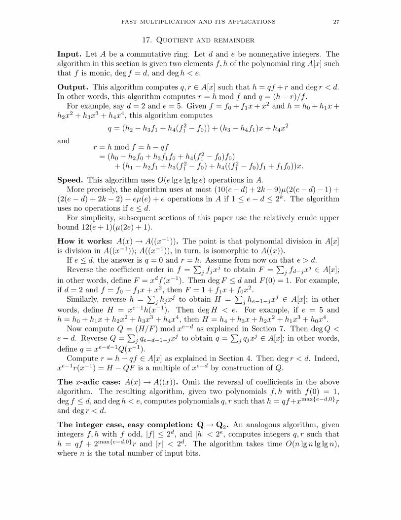
Input. Let A be a commutative ring. Let d and e be nonnegative integers. Thealgorithm in this section is given two elements f, h of the polynomial ring A[x] suchthat f is monic, deg f = d, and deg h < e.
Output. This algorithm computes q, r ∈ A[x] such that h = qf + r and deg r < d.In other words, this algorithm computes r = h mod f and q = (h − r)/f .
For example, say d = 2 and e = 5. Given f = f0 + f1x + x2 and h = h0 + h1x +h2x
2 + h3x3 + h4x
4, this algorithm computes
q = (h2 − h3f1 + h4(f21 − f0)) + (h3 − h4f1)x + h4x
2
andr = h mod f = h − qf
= (h0 − h2f0 + h3f1f0 + h4(f21 − f0)f0)
+ (h1 − h2f1 + h3(f21 − f0) + h4((f
21 − f0)f1 + f1f0))x.
Speed. This algorithm uses O(e lg e lg lg e) operations in A.More precisely, the algorithm uses at most (10(e− d) + 2k − 9)µ(2(e− d)− 1) +
(2(e − d) + 2k − 2) + eµ(e) + e operations in A if 1 ≤ e − d ≤ 2k. The algorithmuses no operations if e ≤ d.
For simplicity, subsequent sections of this paper use the relatively crude upperbound 12(e + 1)(µ(2e) + 1).
How it works: A(x) → A((x−1)). The point is that polynomial division in A[x]is division in A((x−1)); A((x−1)), in turn, is isomorphic to A((x)).
If e ≤ d, the answer is q = 0 and r = h. Assume from now on that e > d.Reverse the coefficient order in f =
∑
j fjxj to obtain F =
∑
j fd−jxj ∈ A[x];
in other words, define F = xdf(x−1). Then deg F ≤ d and F (0) = 1. For example,if d = 2 and f = f0 + f1x + x2, then F = 1 + f1x + f0x
2.Similarly, reverse h =
∑
j hjxj to obtain H =
∑
j he−1−jxj ∈ A[x]; in other
words, define H = xe−1h(x−1). Then deg H < e. For example, if e = 5 andh = h0 + h1x + h2x
2 + h3x3 + h4x
4, then H = h4 + h3x + h2x2 + h1x
3 + h0x4.
Now compute Q = (H/F ) mod xe−d as explained in Section 7. Then deg Q <e − d. Reverse Q =
∑
j qe−d−1−jxj to obtain q =
∑
j qjxj ∈ A[x]; in other words,
define q = xe−d−1Q(x−1).Compute r = h − qf ∈ A[x] as explained in Section 4. Then deg r < d. Indeed,
xe−1r(x−1) = H − QF is a multiple of xe−d by construction of Q.
The x-adic case: A(x) → A((x)). Omit the reversal of coefficients in the abovealgorithm. The resulting algorithm, given two polynomials f, h with f(0) = 1,deg f ≤ d, and deg h < e, computes polynomials q, r such that h = qf+xmax{e−d,0}rand deg r < d.
The integer case, easy completion: Q → Q2. An analogous algorithm, givenintegers f, h with f odd, |f | ≤ 2d, and |h| < 2e, computes integers q, r such thath = qf + 2max{e−d,0}r and |r| < 2d. The algorithm takes time O(n lg n lg lg n),where n is the total number of input bits.
28 DANIEL J. BERNSTEIN
The integer case, hard completion: Q → R. An analogous algorithm, givenintegers f, h with f 6= 0, computes integers q, r such that h = qf+r and 0 ≤ r < |f |.The algorithm takes time O(n lg n lg lg n), where n is the total number of input bits.
It is often convenient to change the sign of r when f is negative; in other words,to replace 0 ≤ r < |f | with 0 ≤ r/f < 1; in other words, to take q = bh/fc. Thetime remains O(n lg n lg lg n).
History. See Section 7 for historical notes on fast division in A[[x]] and R.The use of x 7→ x−1 for computing quotients dates back to at least 1973: Strassen
commented in [111, page 240] (translated) that “the division of two formal powerseries can easily be used for the division of two polynomials with remainder.” Ihave not attempted to trace the earlier history of the x−1 valuation.
Improvements. One can often save some time, particularly in the integer case,by changing the problem, allowing a wider range of remainders. Most applicationsdo not need the smallest possible remainder of h modulo f ; any reasonably smallremainder is adequate.
A different way to divide h by f is to recursively divide the top half of h bythe top half of f , then recursively divide what’s left. Moenck and Borodin in[85] published this algorithm (in the polynomial case), and observed that it takestime O(n(lg n)2 lg lg n). Later, in [20, Section 6], Borodin and Moenck summarizedthe idea in two sentences and then dismissed it in favor of multiply-by-reciprocal.The Moenck-Borodin idea was reinvented many years later (in the integer case) byJebelean in [62], by Daniel Ford (according to email I received from John Cannonin June 1998), and by Burnikel and Ziegler in [35]. The idea is claimed in [35,Section 4] to be faster than multiply-by-reciprocal for fairly large values of n; onthe other hand, the algorithm in [35, Section 4.2] is certainly not the state of theart in reciprocal computation. Further investigation is needed.
Many applications of division in R can work equally well with division in Z2.This fact—widely known to number theorists since Hensel’s introduction of Z2
(and more general completions) in the early 1900s—has frequently been applied tocomputations; replacing R with Z2 usually saves a little time and a considerableamount of effort. See, e.g., [78], [55], [52], [43] (using Zp where, for simplicity,p is chosen to not divide an input), [86], and [61]. Often Z2 division is called“Montgomery reduction,” but this gives too much credit to [86].
In some applications, one knows in advance that a division will be exact, i.e.,that the remainder will be zero. Schonhage and Vetter in [103] suggested computingthe top half of the quotient with division in R, and the bottom half of the quotientwith division in Z2. These two half-size computations are faster than one full-size computation, because computation speed is not exactly linear. Similarly, forpolynomials, one can combine x-adic division with the usual division.
Another exact-division method, for h, f ∈ C[x], is deconvolution: one solvesh = qf by transforming h, transforming f , dividing to obtain the transform of q,and untransforming the result to obtain q. Extra work is required if the transformof f is noninvertible.
FAST MULTIPLICATION AND ITS APPLICATIONS 29
18. Remainder tree
Input. Let A be a commutative ring. Let t be a nonnegative integer. The al-gorithm in this section is given a polynomial h ∈ A[x] and monic polynomialsf1, f2, . . . , ft ∈ A[x].
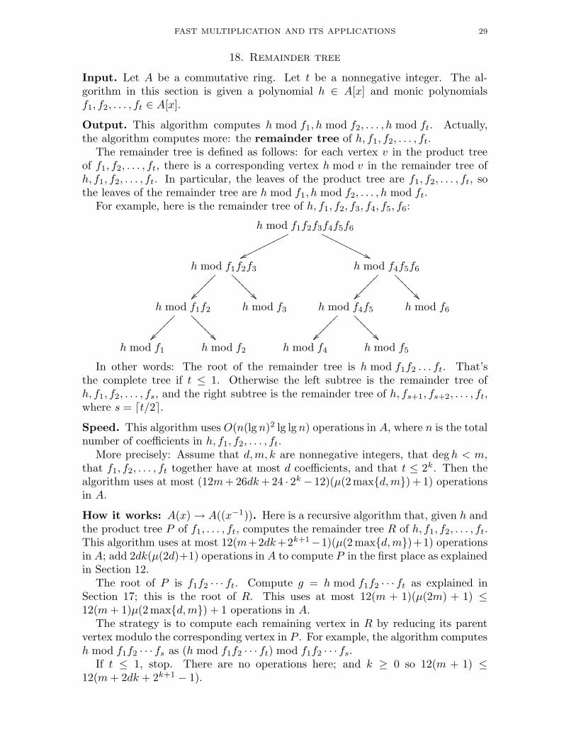
Output. This algorithm computes h mod f1, h mod f2, . . . , h mod ft. Actually,the algorithm computes more: the remainder tree of h, f1, f2, . . . , ft.
The remainder tree is defined as follows: for each vertex v in the product treeof f1, f2, . . . , ft, there is a corresponding vertex h mod v in the remainder tree ofh, f1, f2, . . . , ft. In particular, the leaves of the product tree are f1, f2, . . . , ft, sothe leaves of the remainder tree are h mod f1, h mod f2, . . . , h mod ft.
For example, here is the remainder tree of h, f1, f2, f3, f4, f5, f6:
h mod f1f2f3f4f5f6
h mod f1f2f3
ww
oooooooooo
h mod f4f5f6
''
OOOOOOOOOO
h mod f1f2
��
�������
h mod f3
��
???????
h mod f4f5
��
�������
h mod f6
��
???????
h mod f1
��
�������
h mod f2
��
???????
h mod f4
��
�������
h mod f5
��
???????
In other words: The root of the remainder tree is h mod f1f2 . . . ft. That’sthe complete tree if t ≤ 1. Otherwise the left subtree is the remainder tree ofh, f1, f2, . . . , fs, and the right subtree is the remainder tree of h, fs+1, fs+2, . . . , ft,where s = dt/2e.Speed. This algorithm uses O(n(lg n)2 lg lg n) operations in A, where n is the totalnumber of coefficients in h, f1, f2, . . . , ft.
More precisely: Assume that d,m, k are nonnegative integers, that deg h < m,that f1, f2, . . . , ft together have at most d coefficients, and that t ≤ 2k. Then thealgorithm uses at most (12m + 26dk + 24 · 2k − 12)(µ(2max{d,m}) + 1) operationsin A.
How it works: A(x) → A((x−1)). Here is a recursive algorithm that, given h andthe product tree P of f1, . . . , ft, computes the remainder tree R of h, f1, f2, . . . , ft.This algorithm uses at most 12(m+2dk+2k+1−1)(µ(2max{d,m})+1) operationsin A; add 2dk(µ(2d)+1) operations in A to compute P in the first place as explainedin Section 12.
The root of P is f1f2 · · · ft. Compute g = h mod f1f2 · · · ft as explained inSection 17; this is the root of R. This uses at most 12(m + 1)(µ(2m) + 1) ≤12(m + 1)µ(2max{d,m}) + 1 operations in A.
The strategy is to compute each remaining vertex in R by reducing its parentvertex modulo the corresponding vertex in P . For example, the algorithm computesh mod f1f2 · · · fs as (h mod f1f2 · · · ft) mod f1f2 · · · fs.
If t ≤ 1, stop. There are no operations here; and k ≥ 0 so 12(m + 1) ≤12(m + 2dk + 2k+1 − 1).
30 DANIEL J. BERNSTEIN
Otherwise define s = dt/2e. Apply this algorithm recursively to g and the leftsubtree of P to compute the remainder tree of g, f1, f2, . . . , fs, which is exactly theleft subtree of R. Apply this algorithm recursively to g and the right subtree ofP to compute the remainder tree of g, fs+1, fs+2, . . . , ft, which is exactly the rightsubtree of R.
Time analysis: Define c as the number of coefficients of f1, . . . , fs. By induction,the recursion for the left subtree uses at most 12(d + 2c(k − 1) + 2k − 1) timesµ(2d) + 1 ≤ µ(2max{d,m}) + 1 operations, since deg g < d. The recursion for theright subtree uses at most 12(d+2(d− c)(k−1)+2k −1) times µ(2max{d,m})+1operations. Add: m + 1 + d + 2c(k − 1) + 2k − 1 + d + 2(d − c)(k − 1) + 2k − 1 =m + 2dk + 2k+1 − 1.
The x-adic case: A(x) → A((x)). One obtains a simpler algorithm by omittingthe reversals described in Section 17. The simpler algorithm, given polynomialsh, f1, f2, . . . , ft where f1(0) = f2(0) = · · · = ft(0) = 1, computes small polynomialsr1, r2, . . . , rt such that h is congruent modulo fj to a certain power of x times rj .The algorithm uses O(n(lg n)2 lg lg n) operations in A.
The integer case, easy completion: Q → Q2. An analogous algorithm, givenan integer h and odd integers f1, f2, . . . , ft, computes small integers r1, r2, . . . , rt
such that h is congruent modulo fj to a certain power of 2 times rj . The algorithmtakes time O(n(lg n)2 lg lg n), where n is the total number of input bits.
The integer case, hard completion: Q → R. An analogous algorithm, givenan integer h and nonzero integers f1, f2, . . . , ft, computes integers r1, r2, . . . , rt,with 0 ≤ rj < |fj |, such that h is congruent modulo fj to rj . The algorithm takestime O(n(lg n)2 lg lg n), where n is the total number of input bits.
History. This algorithm was published by Borodin and Moenck in [85] and [20,Sections 4–6] for “single-precision” moduli f1, f2, . . . , ft.
Improvements. Montgomery in [87, Section 3.7] pointed out several opportunitiesto remove redundancy—for example, by FFT caching—within and across levels ofcomputation of a remainder tree.
One can replace the remainder tree with the scaled remainder tree to saveanother constant factor in the computation of h mod f1, h mod f2, . . . , h mod ft.Where the remainder tree has integers such as h mod f1f2, the scaled remainder treehas real numbers such as (h mod f1f2)/f1f2, represented in the usual way as nearbyfloating-point numbers. Here’s the point: moving from h mod f1f2 to h mod f1
means dividing by f1; moving from (h mod f1f2)/f1f2 to (h mod f1)/f1 meansmultiplying by f2, which is faster. This speedup was achieved in the polynomialcase by Bostan, Lecerf, and Schost, using a more complicated approach that doesnot work for integers; see [24] and [23, Section 3.1]. I found the scaled-remainder-tree structure, achieved the same speedup for integers, and then pointed out someredundancies that could be removed, saving even more time. See [19].
FAST MULTIPLICATION AND ITS APPLICATIONS 31
19. Small factors of a product
Input. Let A be a commutative ring. Let s be a positive integer, and let tbe a nonnegative integer. The algorithm in this section is given polynomialsh1, h2, . . . , hs ∈ A[x] and monic polynomials f1, f2, . . . , ft ∈ A[x].
Output. This algorithm figures out which fi’s divide h1h2 · · ·hs: it computes thesubsequence g1, g2, . . . of f1, . . . , ft consisting of each fi that divides h1h2 · · ·hs.
The name “small factors” comes from the following important special case. LetA be a finite field, and let f1, f2, . . . be all the small primes in A[x], i.e., all thelow-degree monic irreducible polynomials in A[x]. Then this algorithm computesthe small factors of h1h2 · · ·hs.
For example, say A = Z/2, s = 4, t = 5, h1 = 101111 = 1 + x2 + x3 + x4 + x5,h2 = 1101011, h3 = 00001011, h4 = 0001111, f1 = 01, f2 = 11, f3 = 111,f4 = 1101, and f5 = 1011. This algorithm finds all the factors of h1h2h3h4 amongf1, f2, f3, f4, f5. Its output is (01, 11, 111, 1011): the product h1h2h3h4 is divisibleby 01, 11, 111, and 1011, but not by 1101.
Speed. This algorithm uses O(n(lg n)2 lg lg n) operations in A, where n is the totalnumber of coefficients in h1, h2, . . . , hs, f1, f2, . . . , ft.
More precisely: Assume that d,m, j, k are nonnegative integers, that h1, . . . , hs
together have at most m coefficients, that f1, . . . , ft together have at most dcoefficients, that s ≤ 2j , and that t ≤ 2k. Then the algorithm uses at most(2mj + 12m + 26dk + 24 · 2k − 12)(µ(2max{d,m}) + 1) + d operations in A.
How it works. Compute h = h1h2 · · · hs as explained in Section 12. This uses atmost 2mj(µ(m) + 1) ≤ 2mj(µ(2max{d,m}) + 1) operations in A.
Compute h mod f1, h mod f2, . . . , h mod ft as explained in Section 18. This usesat most (12m + 26dk + 24 · 2k − 12)(µ(2max{d,m}) + 1) operations in A.
Check whether h mod f1 = 0, h mod f2 = 0, . . . , h mod ft = 0. This uses atmost d equality tests in A.
The integer case. An analogous algorithm, given integers h1, h2, . . . , hs and givennonzero integers f1, f2, . . . , ft, figures out which fi’s divide h1h2 · · · hs. The algo-rithm takes time O(n(lg n)2 lg lg n), where n is the total number of input bits.
History. See Section 20. This algorithm is a stepping-stone to the algorithm ofSection 20.
Improvements. See Section 12 for improved product-tree algorithms, and Section18 for improved remainder-tree algorithms.
As discussed in Section 17, Schonhage and Vetter combined Z2 and R to computea quotient more quickly when the remainder was known in advance to be 0. Asimilar technique can be used to check more quickly whether a remainder is 0.
32 DANIEL J. BERNSTEIN
20. Small factors of a sequence
Input. Let A be a commutative ring. Let s be a positive integer, and let t be anonnegative integer. The algorithm in this section is given nonzero polynomialsh1, h2, . . . , hs ∈ A[x] and monic coprime polynomials f1, f2, . . . , ft ∈ A[x] withdeg fi ≥ 1 for each i.
Here coprime means that A[x] = fiA[x] + fjA[x] for every i, j with i 6= j;in other words, there exist u, v ∈ A[x] with fiu + fjv = 1. (Warning: Someauthors instead say pairwise coprime, reserving “coprime” for the notion thatA[x] = f1A[x] + f2A[x] + · · · + ftA[x].)
The importance of coprimality is the Chinese remainder theorem: the A[x]-algebra morphism from A[x]/f1f2 · · · ft to A[x]/f1 × A[x]/f2 × · · · × A[x]/ft is anisomorphism. In particular, if each of f1, f2, . . . , ft divides a polynomial h, thenthe product f1f2 · · · ft divides h. This is crucial for the speed of the algorithm.
Output. This algorithm figures out which fi’s divide h1, which fi’s divide h2,which fi’s divide h3, etc.
As in Section 19, the name “small factors” comes from the important specialcase that A is a finite field and f1, f2, . . . are all of the small primes in A[x]. Thenthis algorithm computes the small factors of h1, the small factors of h2, etc.
For example, say A = Z/2, s = 4, t = 5, h1 = 101111 = 1 + x2 + x3 + x4 + x5,h2 = 1101011, h3 = 00001011, h4 = 0001111, f1 = 01, f2 = 11, f3 = 111,f4 = 1101, and f5 = 1011. This algorithm finds all the factors of h1, h2, h3, h4
among f1, f2, f3, f4, f5. Its output is (), (111), (01, 1011), (01, 11).
Speed. This algorithm uses O(n(lg n)3 lg lg n) operations in A, where n is the totalnumber of coefficients in h1, h2, . . . , hs, f1, f2, . . . , ft.
More precisely: Assume, as in Section 19, that d,m, j, k are nonnegative integers,that h1, . . . , hs together have at most m coefficients, that f1, . . . , ft together haveat most d coefficients, that s ≤ 2j , and that t ≤ 2k. Then the algorithm uses atmost ((104jk + j2 + 109j + 12)m + 26dk + 24 · 2k)(µ(2max{d,m}) + 1) + d + 4mjoperations in A.
How it works. Figure out which of f1, f2, . . . , ft divide h1h2 · · · hs, as explainedin Section 19. Write (g1, g2, . . . ) for this subsequence of (f1, f2, . . . , ft). This uses atmost (2mj +12m+26dk+24 ·2k)(µ(2max{d,m})+1)+d operations in A, leaving(104jk+j2 +107j)m(µ(2max{d,m})+1)+4mj operations for the remaining stepsin the algorithm.
If s = 1, the answer is (g1, g2, . . . ). There are no further operations in this case,and (104jk + j2 + 107j)m(µ(2max{d,m}) + 1) + 4mj is nonnegative.
Otherwise apply the algorithm recursively to h1, h2, . . . , hr and g1, g2, . . . , andthen apply the algorithm recursively to hr+1, hr+2, . . . , hs and g1, g2, . . . , wherer = ds/2e. This works because any f ’s that divide hi also divide h1h2 · · ·hs andare therefore included among the g’s.
The central point in the time analysis is that deg(g1g2 · · · ) < m. Indeed,g1, g2, . . . are coprime divisors of h1 · · · hs, so their product is a divisor of h1 · · ·hs;but h1 · · ·hs is a nonzero polynomial of degree smaller than m. Thus there are atmost min{m, t} polynomials in g1, g2, . . . , and the total number of coefficients ing1, g2, . . . is at most min{2m, d}.
FAST MULTIPLICATION AND ITS APPLICATIONS 33
Define ` as the number of coefficients in h1, h2, . . . , hr, and define e as the smallestnonnegative integer with min{m, t} ≤ 2e. Then ` ≤ m; e ≤ k; and 2e ≤ 2m, sincem ≥ 1. By induction, the recursive computation for h1, . . . , hr, g1, g2, . . . uses atmost
((104(j − 1)e + (j − 1)2 + 109(j − 1) + 12)` + 26min{2m, d}e + 24 · 2e)(µ(2max{min{2m, d}, `}) + 1) + min{2m, d} + 4`(j − 1)
≤ ((104(j − 1)k + (j − 1)2 + 109(j − 1) + 12)` + 52mk + 48m)(µ(2max{d,m}) + 1) + 2m + 4`(j − 1)
operations in A. Similarly, the recursive computation for hr+1, . . . , hs, g1, g2, . . .uses at most
((104(j − 1)k + (j − 1)2 + 109(j − 1) + 12)(m − `) + 52mk + 48m)(µ(2max{d,m}) + 1) + 2m + 4(m − `)(j − 1)
operations in A. The total is exactly (104jk+j2+107j)m(µ(2max{d,m})+1)+4mjas desired.
Here is an example of how the algorithm works. To factor h1 = 101111,h2 = 1101011, h3 = 00001011, and h4 = 0001111 over A = Z/2 using theprimes 01, 11, 111, 1101, 1011, the algorithm first finds the factors 01, 11, 111, 1011of h1h2h3h4 as explained in Section 19. It then recursively factors h1, h2 using01, 11, 111, 1011, and recursively factors h3, h4 using 01, 11, 111, 1011.
At the first level of recursion in the same example: To factor h3, h4 using01, 11, 111, 1011, the algorithm finds the factors 01, 11, 1011 of h3h4 as explained inSection 19. It then recursively factors h3 using 01, 11, 1011, and recursively factorsh4 using 01, 11, 1011.
The integer case. An analogous algorithm, given nonzero integers h1, h2, . . . , hs
and coprime integers f1, f2, . . . , ft ≥ 2, figures out which fj ’s divide h1, which fj ’sdivide h2, which fj ’s divide h3, etc. The algorithm takes time O(n(lg n)3 lg lg n),where n is the total number of input bits.
An important special case is that f1, f2, . . . , ft are the first t prime numbers.Then this algorithm computes the small factors of h1, the small factors of h2, etc.
History. I introduced this algorithm in [12, Section 21] and [14]. The version in[12] is slower but more general: it relies solely on multiplication, exact division, andgreatest common divisors.
Improvements. There are many previous algorithms to find small factors: forexample, Legendre’s root-finding method (when the inputs are polynomials overa finite field), sieving (when the inputs are successive values of a polynomial),Pollard’s p− 1 method, and Lenstra’s elliptic-curve method. See [14, Section 2] fora survey. One of my current projects is to combine and optimize these algorithms.
Many applications—see [14, Section 3], for example, and Chapter 11 of thisbook—discard inputs that are not smooth, i.e., that do not factor completelyover the primes f1, f2, . . . , ft. One can identify and discard those inputs withoutfactoring them. Franke, Kleinjung, Morain, and Wirth in [48, Section 4] publisheda smoothness-detection algorithm that typically takes time O(n(lg n)2 lg lg n). Mypaper [18] explains a slight variant that always takes time O(n(lg n)2 lg lg n): firstcompute f = f1f2 · · · ft; then compute f mod h1, f mod h2, . . . ; then, for each i,
compute f2bi
mod hi by repeated squaring, for a sensible choice of bi. The resultis 0 if and only if hi is smooth.
34 DANIEL J. BERNSTEIN
21. Continued fraction from fraction
Input. Let A be a field. Let d be a nonnegative integer. The algorithm in thissection is given polynomials f1, f2 ∈ A[x], not both zero.
Both f1 and f2 are assumed to be represented without leading zero coefficients,so the algorithm can see the degrees of f1 and f2 without any equality tests in A.
Output. This algorithm computes polynomials M11,M12,M21,M22 in A[x] suchthat deg M11,deg M12,deg M21,deg M22 are all at most d; M11M22 − M12M21 isin {−1, 1}; and deg(M21f1 + M22f2) < max{deg f1,deg f2} − d. In particular,M21f1 + M22f2 = 0 in the important special case d = max{deg f1,deg f2}.
This algorithm also computes a factorization of the matrix M =
(
M11 M12
M21 M22
)
:
polynomials q1, q2, . . . , qt ∈ A[x] with M =
(
0 11 −qt
)
· · ·(
0 11 −q2
)(
0 11 −q1
)
. In
particular,
(
f1
f2
)
=
(
q1 11 0
)(
q2 11 0
)
· · ·(
qt 11 0
)
M
(
f1
f2
)
. The reader may think
of this equation as expanding f1/f2 into a continued fraction
q1 +1
q2 +1
. . . +1
qt +g2
g1
with g1 = M11f1 + M12f2 and g2 = M21f1 + M22f2; see Section 14.Note for future reference that if deg f1 ≥ deg f2 then deg g1 = deg f1−deg M22 ≥
deg f1 − d > deg g2; if also M21 6= 0 then deg g1 = deg f2 − deg M21. (Proof:deg M12g2 < d + deg f1 − d = deg f1, and M22g1 = M12g2 ± f1, so deg M22g1 =deg f1. If M21 6= 0 then deg M21f1 ≥ deg f1 ≥ deg f1 − d > deg g2, and M22f2 =g2 − M21f1, so deg M22f2 = deg M21f1.)
Speed. This algorithm uses O(d(lg d)2 lg lg d) operations in A.More precisely: Assume that 2d ≤ 2k where k is a nonnegative integer. Then
this algorithm uses at most (46dk + 44(2k+1 − 1))(µ(4d + 8) + 1) operations in A.This bound is pessimistic.
How it works. The desired matrix M is computed in nine steps shown below.The desired factorization of M is visible from the construction of M , as is the(consequent) fact that detM ∈ {−1, 1}.
There are several recursive calls in this algorithm. Most of the recursive callsreduce d; the other recursive calls preserve d and reduce deg f2. The time analysisinducts on (d,deg f2) in lexicographic order.
Step 1: fix the input order. If deg f1 < deg f2: Apply the algorithm recursivelyto d, f2, f1 to find a matrix C, of degree at most d, such that deg(C21f2 +C22f1) <
deg f2 − d. Compute M = C
(
0 11 0
)
. The answer is M .
Time analysis: By induction, the recursive computation of C uses at most(46dk + 44(2k+1 − 1))(µ(4d + 8) + 1) operations. The computation of M usesno operations: M is simply a reshuffling of C.
FAST MULTIPLICATION AND ITS APPLICATIONS 35
Step 2: check for large d. If deg f1 < d: Apply the algorithm recursively todeg f1, f1, f2 to find a matrix M , of degree at most deg f1 < d, such that M21f1 +M22f2 = 0. The answer is M .
Time analysis: By induction, the recursive computation of M uses at most(46(deg f1)k+44(2k+1−1))(µ(4(deg f1)+8)+1) ≤ (46dk+44(2k+1−1))(µ(4d+8)+1)operations.
Step 3: if no quotients are needed, stop. If deg f2 < deg f1 − d: The answer
is
(
1 00 1
)
.
Time analysis: This computation uses 0 ≤ (46dk + 44(2k+1 − 1))(µ(4d + 8) + 1)operations.
Step 4: focus on the top 2d coefficients. Define i = deg f1 − 2d. If i > 0:Apply the algorithm recursively to d,
⌊
f1/xi⌋
,⌊
f2/xi⌋
to find a matrix M , of degree
at most d, such that deg(M21
⌊
f1/xi⌋
+M22
⌊
f2/xi⌋
) < deg(⌊
f1/xi⌋
)−d = deg f1 −i − d.
The answer is M . Indeed, xi(M21
⌊
f1/xi⌋
+ M22
⌊
f2/xi⌋
) has degree below
deg f1−d; M21(f1 mod xi) and M22(f2 mod xi) have degree below d+i = deg f1−d;add to see that M21f1 + M22f2 has degree below deg f1 − d.
Time analysis: By induction, the recursive computation of M uses at most(46dk + 44(2k+1 − 1))(µ(4d + 8) + 1) operations as claimed.
From now on, 0 ≤ deg f1 − d ≤ deg f2 ≤ deg f1 ≤ 2d.
Step 5: handle degree 0. If d = 0 then deg f1 = deg f2 = 0; the answer is(
0 11 −f1/f2
)
.
Time analysis: This computation uses 2 ≤ (46dk + 44(2k+1 − 1))(µ(4d + 8) + 1)operations as claimed.
From now on, d ≥ 1, so k ≥ 1.
Step 6: compute the first half of the continued fraction. Find a matrix C,of degree at most bd/2c, with deg(C21f1 + C22f2) < deg f1 − bd/2c, by applyingthis algorithm to bd/2c , f1, f2. Compute g2 = C21f1 + C22f2. Compute deg g2.
Time analysis: Note that 2 bd/2c ≤ d ≤ 2k−1. The recursive computation of Cuses at most (46(d/2)(k−1)+44(2k−1))(µ(4(d/2)+8)+1) operations by induction.The computation of C21f1 uses at most 3dµ(3d) operations, since deg C21 ≤ d anddeg f1 ≤ 2d. The computation of C22f2 uses at most 3dµ(3d) operations. Thecomputation of g2 uses at most 2d additions, since deg g2 < deg f1 ≤ 2d. Thecomputation of deg g2 uses at most 2d equality tests.
Step 7: if no more quotients are needed, stop. If deg g2 < deg f1 − d: Theanswer is C. Time analysis: There are no operations here; for comparison, morethan 0 operations are counted below.
From now on, deg f1 − d ≤ deg g2 < deg f1 − bd/2c.Step 8: compute one more quotient. Compute g1 = C11f1 +C12f2. Computepolynomials q, r ∈ A[x] such that g1 = qg2 + r and deg r < deg g2, as explained inSection 17. Compute deg r.
Problem: Section 17 considers division by monic polynomials; g2 is usually notmonic. Solution: Divide g2 by its leading coefficient, and adjust q accordingly.
36 DANIEL J. BERNSTEIN
Observe that the matrix
(
0 11 −q
)
C =
(
C21 C22
C11 − qC21 C12 − qC22
)
has degree
at most deg f1−deg g2. (Proof: Recall that deg C22 = deg f1−deg g1; so deg qC22 =deg q + deg C22 = (deg g1 − deg g2) + (deg f1 − deg g1) = deg f1 − deg g2. Recallalso that deg C21 ≤ deg f2 −deg g1 ≤ deg f1 −deg g1; so deg qC21 ≤ deg f1 −deg g2.Finally, all of C11, C12, C21, C22 have degree at most bd/2c < deg f1 − deg g2.)
Time analysis: The computation of g1 uses at most 6dµ(3d)+2d+1 operations,since deg g1 ≤ deg f1 ≤ 2d. The division of g2 by its leading coefficient uses at most2d operations. The division of g1 by the result uses at most 12(2d+2)(µ(4d+2)+1)operations. The division of the quotient by the leading coefficient of g2 uses at mostd + 1 operations since deg q ≤ deg f1 − deg g2 ≤ d. The computation of deg r usesat most 2d equality tests.
Step 9: compute the second half of the continued fraction. Find a matrixD, of degree at most deg g2−(deg f1−d), such that deg(D21g2+D22r) < deg f1−d,by applying the algorithm recursively to deg g2 − (deg f1 − d), g2, r.
Compute M = D
(
0 11 −q
)
C. Observe that M21f1+M22f2 =(
0 1)
M
(
f1
f2
)
=
(
0 1)
D
(
0 11 −q
)
C
(
f1
f2
)
=(
D21 D22
)
(
0 11 −q
)(
g1
g2
)
=(
D21 D22
)
(
g2
r
)
=
D21g2 + D22r.The answer is M . Indeed, the degree of D is at most deg g2 − deg f1 + d, and
the degree of
(
0 11 −q
)
C is at most deg f1 − deg g2, so the degree of M is at most
d; and deg(M21f1 + M22f2) = deg(D21g2 + D22r) < deg f1 − d.Time analysis: Note that deg g2−(deg f1−d) ≤ deg f1−bd/2c−1−(deg f1−d) ≤
bd/2c. By induction, the recursive computation of D uses at most
(46(d/2)(k − 1) + 44(2k − 1))(µ(4(d/2) + 8) + 1)
operations. The computation of qC21 uses at most (d + 1)µ(d + 1) operationssince deg qC21 ≤ deg f1 − deg g2 ≤ d. The computation of qC22 uses at most(d + 1)µ(d + 1) operations since deg qC22 = deg f1 − deg g2 ≤ d. The computationof C11 − qC21 uses at most d + 1 operations. The computation of C12 − qC22 uses
at most d + 1 operations. The multiplication of D by
(
0 11 −q
)
C uses at most
(8d + 16)(µ(4d + 8) + 1) operations.Totals: at most (46d(k − 1) + 44(2k+1 − 2))(µ(4d + 8) + 1) operations for the
recursive computations of C and D, and at most (46d + 42)µ(4d + 8) + 45d + 44 ≤(46d+44)(µ(4d+8)+1) operations for everything else. The grand total is at most(46dk + 44(2k+1 − 1))(µ(4d + 8) + 1) operations as claimed.
The integer case. A more complicated algorithm, given a nonnegative integer dand given integers f1, f2 not both zero, computes a (factored) 2×2 integer matrix Mwith entries not much larger than 2d in absolute value, with determinant in {−1, 1},and with |M21f1 + M22f2| < max{|f1| , |f2|}/2d. It takes time O(n(lg n)2 lg lg n),where n is the total number of input bits.
The main complication here is that the answer for the top 2d bits of f1 and f2
is, in general, not exactly the answer for f1 and f2. One has to check whether|M21f1 + M22f2| is too large, and divide a few more times if it is.
FAST MULTIPLICATION AND ITS APPLICATIONS 37
History. Almost all of the ideas in this algorithm were published by Lehmer in[81] in the integer case. Lehmer made the crucial observation that the top 2d bitsof f1 and f2 determined approximately d bits of the continued fraction for f1/f2.Lehmer suggested computing the continued fraction for f1/f2 by computing a smallpart of the continued fraction, computing another quotient, and then computingthe rest of the continued fraction.
Shortly after fast multiplication was widely understood, Knuth in [70] suggestedreplacing “a small part” with “half” in Lehmer’s algorithm. Knuth proved thatthe continued fraction for f1/f2 could be computed within a O((lg n)4) factor ofmultiplication time. Schonhage in [97] streamlined the Lehmer-Knuth algorithmand proved that the continued fraction for f1/f2 could be computed within a O(lg n)factor of multiplication time.
The (lg n)3 disparity between [70] and [97] arose as follows. Knuth lost one
lg n factor from continually re-multiplying matrices
(
0 11 −q
)
instead of reusing
their products M ; another lg n factor from doing a binary search, again with noreuse of partial results, to determine how much of the continued fraction of f1/f2
matched the continued fraction of⌊
f1/2i⌋
/⌊
f2/2i⌋
; and one more lg n factor froman unnecessarily crude analysis.
Moenck in [84] claimed to have a simplified algorithm covering both the integercase and the polynomial case. In fact, Moenck’s algorithm does not work in theinteger case, does not work in the “nonnormal” situation of a quotient having degreedifferent from 1, and does not work except when deg f1 is a power of 2. The errorsin [84] begin on page 143, where the “degree” function mapping an integer A toblg |A|c is claimed to be a homomorphism.
Brent, Gustavson, and Yun in [29, Section 3] outlined a simplified algorithmfor the polynomial case. Strassen in [113, page 16] stated the remarkably cleanalgorithm shown above (under the assumption deg f1 ≥ deg f2), with one omission:Strassen’s algorithm recurses forever when d = deg f1 = deg f2 = 0.
Improvements. There are many opportunities for FFT caching and FFT additionin this algorithm.
One can replace bd/2c in this algorithm by any integer between 0 and d−1. Theoptimal choice depends heavily on the exact speed of multiplication.
It is often helpful (for applications, and for recursion inside this algorithm) tocompute M21f1 + M22f2, and sometimes M11f1 + M12f2, along with M . Onecan often save time by incorporating these computations into the recursion. Forexample, when M is constructed from D, q, C, one can compute M21f1 + M22f2 asD21g2 + D22r, and one can compute M11f1 + M12f2 as D11g2 + D12r.
One can often save time by skipping M11 and M21, and working solely withM12,M22,M11f1 + M12f2,M21f1 + M22f2. Applications that need M11 and M21
can use formulas such as M11 = ((M11f1 + M12f2) − M12f2)/f1. In [72, page 343]this observation is credited to Gordon H. Bradley.
Some applications need solely M11f1+M12f2 and M21f1+M22f2. The algorithm,and some of its recursive calls, can be sped up accordingly.
Often f1 and f2 have an easily detected common factor, such as x or x − 1.Dividing out this factor speeds up the algorithm, perhaps enough to justify thecost of checking for the factor in the first place.
38 DANIEL J. BERNSTEIN
22. Greatest common divisor
Input. Let A be a field. The algorithm in this section is given polynomials f1, f2 ∈A[x].
Output. This algorithm computes gcd{f1, f2}: in other words, a polynomial gsuch that gA[x] = f1A[x] + f2A[x] and such that g is monic if it is nonzero.
This algorithm also computes polynomials h1, h2 ∈ A[x], each of degree at mostmax{deg f1,deg f2}, such that g = f1h1 + f2h2.
In particular, if f1 and f2 are coprime, then g = 1; h1 is a reciprocal of f1 modulof2; and h2 is a reciprocal of f2 modulo f1.
Speed. This algorithm uses O(n(lg n)2 lg lg n) operations in A, where n is the totalnumber of coefficients in f1, f2.
How it works. If f1 = f2 = 0 then the answer is 0, 0, 0. Assume from now onthat at least one of f1 and f2 is nonzero.
Define d = max{deg f1,deg f2}. Apply the algorithm of Section 21 to computeM11,M12,M21,M22 in A[x], of degree at most d, with M11M22 − M12M21 = ±1and M21f1 + M22f2 = 0.
Compute u = M11f1 + M12f2. Note that ±f1 = M22u and ∓f2 = M21u, souA[x] = f1A[x] + f2A[x]. In particular, u 6= 0.
Compute g = u/c, h = M11/c, and h2 = M12/c, where c is the leading coefficientof u. Then g is monic, and gA[x] = f1A[x]+f2A[x], so g = gcd{f1, f2}. The answeris g, h1, h2.
The integer case. An analogous algorithm, given integers f1 and f2, computesgcd{f1, f2} and reasonably small integers h1, h2 with gcd{f1, f2} = f1h1 + f2h2. Ittakes time O(n(lg n)2 lg lg n), where n is the total number of input bits.
History. See Section 21. This application has always been one of the primarymotivations for studying the problem of Section 21.
Improvements. See Section 21.The reader may have noticed that Section 21 and this section use division in
A((x−1)) and division in R. What about Q2? Answer: There are several “binary”algorithms to compute greatest common divisors of integers. See, e.g., [106] and[72, pages 338–341; Exercises 4.5.2–38, 4.5.2–39, 4.5.2–40]. Recently, in [107], Stehleand Zimmermann introduced a particuarly clean “binary” gcd algorithm and provedthat it takes time O(n(lg n)2 lg lg n). The Stehle-Zimmermann algorithm, given anodd integer f1 and an even integer f2, expands f1/f2 into what one might calla simple 2-adic continued fraction: a continued fraction with all quotientschosen from the set {±1/2,±1/4,±3/4,±1/8,±3/8,±5/8,±7/8, . . . }. My initialimpression is that this algorithm supersedes all previous work on gcd computation.
FAST MULTIPLICATION AND ITS APPLICATIONS 39
23. Interpolator
Input. Let A be a field. Let t be a nonnegative integer. The algorithm in thissection is given polynomials f1, f2, . . . , ft ∈ A[x] and nonzero coprime polynomialsg1, g2, . . . , gt ∈ A[x].
Output. This algorithm computes h ∈ A[x], with deg h < deg g1g2 · · · gt, such thath ≡ f1 (mod g1), h ≡ f2 (mod g2), . . . , h ≡ ft (mod gt).
In particular, consider the special case that each gj is a monic linear polynomialx − cj . The answer h is a polynomial of degree below t such that h(c1) = f1(c1),h(c2) = f2(c2), . . . , h(ct) = ft(ct). Finding h is usually called interpolation inthis case, and I suggest using the same name for the general case. Another commonname is Chinese remaindering.
Speed. This algorithm uses O(n(lg n)2 lg lg n) operations in A, where n is the totalnumber of input coefficients.
How it works. For t = 0: The answer is 0.Compute G = g1 · · · gt as explained in Section 12.Compute G mod g2
1 , . . . , G mod g2t as explained in Section 18.
Divide each G mod g2j by gj , as explained in Section 17, to obtain (G/gj) mod gj .
Note that G/gj and gj are coprime; thus ((G/gj) mod gj) and gj are coprime.Compute a (reasonably small) reciprocal pj of ((G/gj) mod gj) modulo gj , as
explained in Section 22. Compute qj = fjpj mod gj as explained in Section 17.Now compute h = (q1/g1 + · · ·+ qt/gt)G as explained in Section 13. (Proof that,
modulo gj , this works: h ≡ qj(G/gj) ≡ fjpj(G/gj) ≡ fjpj(G/gj mod gj) ≡ fj .)
The integer case. An analogous algorithm, given integers f1, f2, . . . , ft and givennonzero coprime integers g1, g2, . . . , gt, computes a reasonably small integer h suchthat h ≡ f1 (mod g1), h ≡ f2 (mod g2), . . . , h ≡ ft (mod gt). The algorithm takestime O(n(lg n)2 lg lg n), where n is the total number of input bits.
History. Horowitz in [60] published most of the above algorithm, in the specialcase that each gj is a monic linear polynomial. Horowitz did not have a fast method(for large t) to compute (G/g1) mod g1, . . . , (G/gt) mod gt from G. Moenck andBorodin in [85, page 95] and [20, page 381] suggested the above solution in the(“single-precision”) integer case.
The special case t = 2 was published first by Heindel and Horowitz in [57], alongwith a different essentially-linear-time interpolation algorithm for general t. TheHeindel-Horowitz algorithm is summarized below; it takes time O(n(lg n)3 lg lg n).
Improvements. When gj is a linear polynomial, (G/gj) mod gj has degree 0,so pj is simply 1/((G/gj) mod gj), and qj is (fj mod gj)/((G/gj) mod gj). Moregenerally, whenever gj is very small, the algorithm of this section provides verysmall inputs to the modular-reciprocal algorithm of Section 22.
When gj is a monic linear polynomial, (G/gj) mod gj is the same as G′ modgj , where G′ is the derivative of G. Borodin and Moenck in [20, Sections 8–9]suggested computing G′ mod g1, . . . , G
′ mod gt as explained in Section 18, insteadof computing G mod g2
1 , . . . , G mod g2t .
More generally, if gj and its derivative g′j are coprime, then (G/gj) mod gj is the
same as (g′j)−1G′ mod gj . One can compute G′ mod g1, . . . , G
′ mod gt; compute
each reciprocal (G′)−1 mod gj ; and then compute qj = fjg′j(G
′)−1 mod gj .
40 DANIEL J. BERNSTEIN
Another way to compute (G/gj) mod gj is to first compute G/g1 + · · ·+G/gt asexplained in Section 13, then compute (G/g1 + · · ·+G/gt) mod gj = (G/gj) mod gj
for all j as explained in Section 18. Burgisser, Clausen, and Shokrollahi publishedthis method in [33, pages 77–78].
When t = 2, one can use the algorithm of Section 22 to simultaneously computea reciprocal p2 of g1 = G/g2 modulo g2 and a reciprocal p1 of g2 = G/g1 modulog1. The answer is then (f1p1 mod g1)g2 + (f2p2 mod g2)g1. It might be faster tocompute (f1p1g2 + f2p2g1) mod g1g2.
One can skip the computation of p1 when f1 = 0. One can reduce the generalcase to this case: interpolate 0, f2 − f1, f3 − f1, . . . , ft − f1 and then add f1 to theresult. In particular, for t = 2, the answer is f1 + ((f2 − f1)p2 mod g2)g1, if f1 issmall enough for that answer to be in the right range.
The Heindel-Horowitz algorithm interpolates pairs, then pairs of pairs, etc. Thismay be better than the Horowitz-Borodin-Moenck algorithm for small t.
One can cache the reciprocals pj for subsequent interpolations involving the sameg1, . . . , gt.
FAST MULTIPLICATION AND ITS APPLICATIONS 41
24. Coprime base
Input. Let A be a field. Let t be a nonnegative integer. The algorithm in thissection is given monic polynomials f1, f2, . . . , ft ∈ A[x].
Output. This algorithm computes a coprime base for {f1, f2, . . . , ft}: coprimemonic polynomials g1, g2, . . . ∈ A[x] such that each fj can be factored as a productof powers of g1, g2, . . . .
In fact, the algorithm computes the natural coprime base for {f1, f2, . . . , ft}:the unique coprime base that does not contain 1 and that can be obtained fromf1, f2, . . . , ft by multiplication, exact division, and greatest common divisors.
In most applications, one also wants the factorization of each fj over g1, g2, . . . .These factorizations can be computed quickly by an extension of the algorithm ofSection 20.
Speed. This algorithm uses O(n(lg n)7 lg lg n) operations in A, where n is the totalnumber of input coefficients.
How it works. See [12]. The algorithm is too complicated to be stated in thispaper, as the reader might guess from the exponent 7.
The integer case. An analogous algorithm computes the natural coprime base ofa set of positive integers f1, f2, . . . , ft. It takes time O(n(lg n)7 lg lg n), where n isthe total number of input bits.
History. I published this algorithm in [12]. No previous essentially-linear-timealgorithms were known, even in the case t = 2.
Improvements. One of my current projects is to speed up this algorithm. I haverecently convinced myself that the natural coprime base can be computed in timeO(n(lg n)4 lg lg n).
42 DANIEL J. BERNSTEIN
References
[1] —, AFIPS conference proceedings, volume 17: 1960 Western Joint Computer Conference,1960. ISSN 0095–6880.
[2] —, AFIPS conference proceedings, volume 28: 1966 Spring Joint Computer Conference,Spartan Books, Washington, 1966.
[3] —, AFIPS conference proceedings, volume 29: 1966 Fall Joint Computer Conference, Spar-tan Books, Washington, 1966.
[4] —, AFIPS conference proceedings, volume 33, part one: 1968 Fall Joint Computer Confer-
ence, December 9–11, 1968, San Francisco, California, Thompson Book Company, Wash-ington, 1968.
[5] —, Actes du congres international des mathematiciens, tome 3, Gauthier-Villars Editeur,Paris, 1971. MR 54:5.
[6] Alfred V. Aho (chairman), Proceedings of fifth annual ACM symposium on theory of com-
puting: Austin, Texas, April 30–May 2, 1973, Association for Computing Machinery, NewYork, 1973.
[7] Robert S. Anderssen, Richard P. Brent (editors), The complexity of computational prob-
lem solving, University of Queensland Press, Brisbane, 1976. ISBN 0–7022–1213–X. URL:http://web.comlab.ox.ac.uk/oucl/work/richard.brent/pub/pub031.html.
[8] Michael Beeler, R. William Gosper, Richard Schroeppel, HAKMEM, Artificial IntelligenceMemo No. 239, Massachusetts Institute of Technology, 1972. URL: http://www.inwap.com/
pdp10/hbaker/hakmem/hakmem.html.[9] Glenn D. Bergland, A fast Fourier transform algorithm for real-valued series, Communi-
cations of the ACM 11 (1968), 703–710. ISSN 0001–0782. URL: http://cr.yp.to/bib/
entries.html#1968/bergland-real.
[10] Daniel J. Bernstein, New fast algorithms for π and e, paper for the Westinghouse compe-tition, distributed widely at the Ramanujan Centenary Conference (1987). URL: http://cr.yp.to/bib/entries.html#1987/bernstein.
[11] Daniel J. Bernstein, Detecting perfect powers in essentially linear time, Mathematics of
Computation 67 (1998), 1253–1283. ISSN 0025–5718. MR 98j:11121. URL: http://cr.yp.to/papers.html.
[12] Daniel J. Bernstein, Factoring into coprimes in essentially linear time, to appear, Journalof Algorithms. ISSN 0196–6774. URL: http://cr.yp.to/papers.html. ID f32943f0bb67a9
317d4021513f9eee5a.[13] Daniel J. Bernstein, Multidigit multiplication for mathematicians. URL: http://cr.yp.to/
papers.html.[14] Daniel J. Bernstein, How to find small factors of integers, accepted to Mathematics of
Computation; now being revamped. URL: http://cr.yp.to/papers.html.[15] Daniel J. Bernstein, Removing redundancy in high-precision Newton iteration, draft. URL:
http://cr.yp.to/papers.html#fastnewton. ID def7f1e35fb654671c6f767b16b93d50.[16] Daniel J. Bernstein, Pippenger’s exponentiation algorithm, to be incorporated into author’s
High-speed cryptography book. URL: http://cr.yp.to/papers.html.[17] Daniel J. Bernstein, Computing logarithm intervals with the arithmetic-geometric-mean it-
eration. URL: http://cr.yp.to/papers.html#logagm. ID 8f92b1e3ec7918d37b28b9efcee5e
97f.
[18] Daniel J. Bernstein, How to find smooth parts of integers, draft. URL: http://cr.yp.to/papers.html#smoothparts. ID 201a045d5bb24f43f0bd0d97fcf5355a.
[19] Daniel J. Bernstein, Scaled remainder trees, draft. URL: http://cr.yp.to/papers.
html#scaledmod. ID e2b8da026cf72d01d97e20cf2874f278.
[20] Allan Borodin, Robert T. Moenck, Fast modular transforms, Journal of Computer andSystem Sciences 8 (1974), 366–386; older version, not a subset, in [85]. ISSN 0022–0000.MR 51:7365. URL: http://cr.yp.to/bib/entries.html#1974/borodin.
[21] Jonathan M. Borwein, Peter B. Borwein, Pi and the AGM, Wiley, New York, 1987. ISBN
0–471–83138–7. MR 89a:11134.[22] Jonathan M. Borwein, David M. Bradley, Richard E. Crandall, Computational strategies
for the Riemann zeta function, Journal of Computational and Applied Mathematics 121
(2000), 247–296. ISSN 0377–0427. MR 2001h:11110. URL: http://www.sciencedirect.com/
science/article/B6TYH-4118GDF-F/1/64371ba75fa0e923ba6b231779fb0673.
FAST MULTIPLICATION AND ITS APPLICATIONS 43
[23] Alin Bostan, Gregoire Lecerf, Bruno Salvy, Eric Schost, Bernd Wiebelt, Complexity issues
in bivariate polynomial factorization, in [95] (2004), 42–49.
[24] Alin Bostan, Gregoire Lecerf, Eric Schost, Tellegen’s principle into practice, in [59] (2003),
37–44.[25] Alfred Brauer, On addition chains, Bulletin of the American Mathematical Society 45
(1939), 736–739. ISSN 0273–0979. MR 1,40a. URL: http://cr.yp.to/bib/entries.html#1939/brauer.
[26] Richard P. Brent, The complexity of multiple-precision arithmetic, in [7] (1976), 126–165.URL: http://web.comlab.ox.ac.uk/oucl/work/richard.brent/pub/pub032.html.
[27] Richard P. Brent, Fast multiple-precision evaluation of elementary functions, Journal ofthe ACM 23 (1976), 242–251. ISSN 0004–5411. MR 52:16111. URL: http://web.comlab.
ox.ac.uk/oucl/work/richard.brent/pub/pub034.html.[28] Richard P. Brent, Multiple-precision zero-finding methods and the complexity of elementary
function evaluation, in [116] (1976), 151–176. MR 54:11843. URL: http://web.comlab.ox.ac.uk/oucl/work/richard.brent/pub/pub028.html.
[29] Richard P. Brent, Fred G. Gustavson, David Y. Y. Yun, Fast solution of Toeplitz systems of
equations and computation of Pade approximants, Journal of Algorithms 1 (1980), 259–295.ISSN 0196–6774. MR 82d:65033. URL: http://web.comlab.ox.ac.uk/oucl/work/richard.brent/pub/pub059.html.
[30] Richard P. Brent, Edwin M. McMillan, Some new algorithms for high-precision compu-
tation of Euler’s constant, Mathematics of Computation 34 (1980), 305–312. ISSN 0025–5718. MR 82g:10002. URL: http://web.comlab.ox.ac.uk/oucl/work/richard.brent/pub/pub049.html.
[31] Georg Bruun, z-transform DFT filters and FFTs, IEEE Transactions on Acoustics, Speech,and Signal Processing 26 (1978), 56–63. ISSN 0096–3518. URL: http://cr.yp.to/bib/
entries.html#1978/bruun.[32] Duncan A. Buell (editor), Algorithmic number theory: 6th international symposium, ANTS-
VI, Burlington, VT, USA, June 2004, proceedings, Lecture Notes in Computer Science,3076, Springer-Verlag, Berlin, 2004. ISBN 3–540–22156–5.
[33] Peter Burgisser, Michael Clausen, Mohammed Amin Shokrollahi, Algebraic complexity the-
ory, Springer-Verlag, Berlin, 1997. ISBN 3–540–60582–7. MR 99c:68002.
[34] Joe P. Buhler (editor), Algorithmic number theory: ANTS-III, Lecture Notes in ComputerScience, 1423, Springer-Verlag, Berlin, 1998. ISBN 3–540–64657–4. MR 2000g:11002.
[35] Christoph Burnikel, Joachim Ziegler, Fast recursive division, MPI research report I-98-1-022,1998. URL: http://data.mpi-sb.mpg.de/internet/reports.nsf/NumberView/1998-1-022.
[36] Jacques Calmet (editor), Computer algebra: EUROCAM ’82, Lecture Notes in ComputerScience, 144, Springer-Verlag, Berlin, 1982. ISBN 3–540–11607–9. MR 83k:68003.
[37] David G. Cantor, Erich Kaltofen, On fast multiplication of polynomials over arbitrary alge-
bras, Acta Informatica 28 (1991), 693–701. ISSN 0001–5903. MR 92i:68068. URL: http://
www.math.ncsu.edu/~kaltofen/bibliography/.[38] David V. Chudnovsky, Gregory V. Chudnovsky, Computer algebra in the service of mathe-
matical physics and number theory, in [39] (1990), 109–232. MR 92g:11122.[39] David V. Chudnovsky, Richard D. Jenks (editors), Computers in mathematics, Lecture
Notes in Pure and Applied Mathematics, 125, Marcel Dekker, New York, 1990. ISBN 0–8247–8341–7. MR 91e:00020.
[40] Stephen A. Cook, On the minimum computation time of functions, Ph.D. thesis, De-partment of Mathematics, Harvard University, 1966. URL: http://cr.yp.to/bib/entries.
html#1966/cook.[41] James W. Cooley, John W. Tukey, An algorithm for the machine calculation of complex
Fourier series, Mathematics of Computation 19 (1965), 297–301. ISSN 0025–5718. MR31:2843. URL: http://cr.yp.to/bib/entries.html#1965/cooley.
[42] Richard Crandall, Barry Fagin, Discrete weighted transforms and large-integer arithmetic,Mathematics of Computation 62 (1994), 305–324. ISSN 0025–5718. MR 94c:11123. URL:http://cr.yp.to/bib/entries.html#1994/crandall.
[43] John D. Dixon, Exact solution of linear equations using p-adic expansions, Numerische
Mathematik 40 (1982), 137–141. ISSN 0029–599X. MR 83m:65025. URL: http://cr.yp.to/bib/entries.html#1982/dixon.
44 DANIEL J. BERNSTEIN
[44] Pierre Duhamel, H. Hollmann, Split-radix FFT algorithm, Electronics Letters 20 (1984),
14–16. ISSN 0013–5194. URL: http://cr.yp.to/bib/entries.html#1984/duhamel.[45] Pierre Duhamel, Martin Vetterli, Fast Fourier transforms: a tutorial review and a state
of the art, Signal Processing 19 (1990), 259–299. ISSN 0165–1684. MR 91a:94004. URL:http://cr.yp.to/bib/entries.html#1990/duhamel.
[46] Gerald Estrin, Organization of computer systems—the fixed plus variable structure com-
puter, in [1] (1960), 33–40. URL: http://cr.yp.to/bib/entries.html#1960/estrin.[47] Charles M. Fiduccia, Polynomial evaluation via the division algorithm: the fast Fourier
transform revisited, in [93] (1972), 88–93. URL: http://cr.yp.to/bib/entries.html#1972/
fiduccia-fft.[48] Jens Franke, T. Kleinjung, Francois Morain, T. Wirth, Proving the primality of very
large numbers with fastECPP. URL: http://www.lix.polytechnique.fr/Labo/Francois.Morain/Articles/large.ps.gz.
[49] Carl F. Gauss, Werke, Band 3, Koniglichen Gesellschaft der Wissenschaften, Gottingen,1866. URL: http://134.76.163.65/agora docs/41929TABLE OF CONTENTS.html.
[50] W. Morven Gentleman, Gordon Sande, Fast Fourier transforms—for fun and profit, in [3](1966), 563–578. URL: http://cr.yp.to/bib/entries.html#1966/gentleman.
[51] William Gosper, Strip mining in the abandoned orefields of nineteenth century mathematics,in [39] (1990), 261–284. MR 91h:11154. URL: http://cr.yp.to/bib/entries.html#1990/gosper.
[52] Robert T. Gregory, Error-free computation: why it is needed and methods for doing
it, Robert E. Krieger Publishing Company, New York, 1980. ISBN 0–89874–240–4. MR83f:65061.
[53] Bruno Haible, Thomas Papanikolaou, Fast multiprecision evaluation of series of ratio-
nal numbers, Technical Report TI-7/97, Darmstadt University of Technology, 1997; see
also newer version [54]. URL: http://www.informatik.tu-darmstadt.de/TI/Mitarbeiter/papanik/Welcome.html.
[54] Bruno Haible, Thomas Papanikolaou, Fast multiprecision evaluation of series of rational
numbers, in [34] (1998), 338–350; see also older version [53]. MR 2000i:11197. URL: http://
cr.yp.to/bib/entries.html#1998/haible.[55] Eric C. R. Hehner, R. Nigel Horspool, A new representation of the rational numbers for
fast easy arithmetic, SIAM Journal on Computing 8 (1979), 124–134. ISSN 0097–5397. MR80h:68027. URL: http://cr.yp.to/bib/entries.html#1979/hehner.
[56] Michael T. Heideman, Don H. Johnson, C. Sidney Burrus, Gauss and the history of the
fast Fourier transform, Archive for History of Exact Sciences 34 (1985), 265–277. ISSN0003–9519. MR 87f:01018. URL: http://cr.yp.to/bib/entries.html#1985/heideman.
[57] Lee E. Heindel, Ellis Horowitz, On decreasing the computing time for modular arithmetic,
in [58] (1971), 126–128. URL: http://cr.yp.to/bib/entries.html#1971/heindel.[58] Fred C. Hennie (chairman), 12th annual symposium on switching and automata theory,
IEEE Computer Society, Northridge, 1971.[59] Hoon Hong (editor), Proceedings of the 2003 international symposium on symbolic and
algebraic computation, Association for Computing Machinery, New York, 2003. ISBN 1–58113–641–2.
[60] Ellis Horowitz, A fast method for interpolation using preconditioning, Information Process-ing Letters 1 (1972), 157–163. ISSN 0020–0190. MR 47:4413. URL: http://cr.yp.to/bib/
entries.html#1972/horowitz.[61] Tudor Jebelean, An algorithm for exact division, Journal of Symbolic Computation 15
(1993), 169–180. ISSN 0747–7171. MR 93m:68092. URL: http://cr.yp.to/bib/entries.html#1993/jebelean.
[62] Tudor Jebelean, Practical integer division with Karatsuba complexity, in [79] (1997), 339–341.
[63] Anatoly A. Karatsuba, Y. Ofman, Multiplication of multidigit numbers on automata, SovietPhysics Doklady 7 (1963), 595–596. ISSN 0038–5689. URL: http://cr.yp.to/bib/entries.
html#1963/karatsuba.[64] Ekatharine A. Karatsuba, Fast evaluation of hypergeometric functions by FEE, in
[91] (1999), 303–314. MR 2000e:65030. URL: http://cr.yp.to/bib/entries.html#1999/
karatsuba.
FAST MULTIPLICATION AND ITS APPLICATIONS 45
[65] Alan H. Karp, Peter Markstein, High-precision division and square root, Technical Re-
port HPL-93-42(R.1), 1994; see also newer version [66]. URL: http://www.hpl.hp.com/
techreports/93/HPL-93-42.html.[66] Alan H. Karp, Peter Markstein, High-precision division and square root, ACM Transac-
tions on Mathematical Software 23 (1997), 561–589; see also older version [65]. ISSN 0098–
3500. MR 1 671 702. URL: http://www.hpl.hp.com/personal/Alan Karp/publications/
publications.html.[67] Richard M. Karp (chairman), 13th annual symposium on switching and automata theory,
IEEE Computer Society, Northridge, 1972.
[68] Donald E. Knuth, The art of computer programming, volume 2: seminumerical algorithms,1st edition, 1st printing, Addison-Wesley, Reading, 1969; see also newer version [69]. MR44:3531.
[69] Donald E. Knuth, The art of computer programming, volume 2: seminumerical algorithms,
1st edition, 2nd printing, Addison-Wesley, Reading, 1971; see also older version [68]; see alsonewer version [71]. MR 44:3531.
[70] Donald E. Knuth, The analysis of algorithms, in [5] (1971), 269–274. MR 54:11839. URL:http://cr.yp.to/bib/entries.html#1971/knuth-gcd.
[71] Donald E. Knuth, The art of computer programming, volume 2: seminumerical algorithms,2nd edition, Addison-Wesley, Reading, 1981; see also older version [69]; see also newerversion [72]. ISBN 0–201–03822–6. MR 83i:68003.
[72] Donald E. Knuth, The art of computer programming, volume 2: seminumerical algorithms,
3rd edition, Addison-Wesley, Reading, 1997; see also older version [71]. ISBN 0–201–89684–2.
[73] Donald E. Knuth (editor), Selected papers on analysis of algorithms, CSLI Publications,Stanford, 2000. ISBN 1–57586–212–3. MR 2001c:68066.
[74] Donald E. Knuth, Christos H. Papadimitriou, Duality in addition chains, Bulletin of theEuropean Association for Theoretical Computer Science 13 (1981), 2–4; reprinted in [73,chapter 31]. ISSN 0252–9742.
[75] Peter M. Kogge, Parallel solution of recurrence problems, IBM Journal of Research and
Development 18 (1974), 138–148. ISSN 0018–8646. MR 49:6552. URL: http://cr.yp.to/bib/entries.html#1974/kogge.
[76] Peter M. Kogge, Harold S. Stone, A parallel algorithm for the efficient solution of a general
class of recurrence equations, IEEE Transactions on Computers 22 (1973), 786–793. ISSN
0018–9340. URL: http://cr.yp.to/bib/entries.html#1973/kogge.[77] Nick Kollerstrom, Thomas Simpson and “Newton’s method of approximation”: an enduring
myth, British Journal for the History of Science 1992 (1992), 347–354. URL: http://www.ucl.ac.uk/sts/nk/newtonapprox.htm.
[78] E. V. Krishnamurthy, Matrix processors using p-adic arithmetic for exact linear computa-
tions, IEEE Transactions on Computers 26 (1977), 633–639. ISSN 0018–9340. MR 57:7963.URL: http://cr.yp.to/bib/entries.html#1977/krishnamurthy.
[79] Wolfgang Kuechlin (editor), Symbolic and algebraic computation: ISSAC ’97, Association
for Computing Machinery, New York, 1997. ISBN 0–89791–875–4.[80] H. T. Kung, On computing reciprocals of power series, Numerische Mathematik 22 (1974),
341–348. ISSN 0029–599X. MR 50:3536. URL: http://cr.yp.to/bib/entries.html#1974/kung.
[81] Derrick H. Lehmer, Euclid’s algorithm for large numbers, American Mathematical Monthly45 (1938), 227–233. ISSN 0002–9890. URL: http://links.jstor.org/sici?sici=0002-9890(193804)45:4<227:EAFLN>2.0.CO;2-Y.
[82] Hendrik W. Lenstra, Jr., Robert Tijdeman (editors), Computational methods in number
theory I, Mathematical Centre Tracts, 154, Mathematisch Centrum, Amsterdam, 1982. ISBN90–6196–248–X. MR 84c:10002.
[83] Jean-Bernard Martens, Recursive cyclotomic factorization—a new algorithm for calculating
the discrete Fourier transform, IEEE Transactions on Acoustics, Speech, and Signal Pro-
cessing 32 (1984), 750–761. ISSN 0096–3518. MR 86b:94004. URL: http://cr.yp.to/bib/entries.html#1984/martens.
[84] Robert T. Moenck, Fast computation of GCDs, in [6] (1973), 142–151. URL: http://cr.yp.to/bib/entries.html#1973/moenck.
46 DANIEL J. BERNSTEIN
[85] Robert T. Moenck, Allan Borodin, Fast modular transforms via division, in [67] (1972),
90–96; newer version, not a superset, in [20]. URL: http://cr.yp.to/bib/entries.html#1972/moenck.
[86] Peter L. Montgomery, Modular multiplication without trial division, Mathematics of Com-putation 44 (1985), 519–521. ISSN 0025–5718. MR 86e:11121.
[87] Peter L. Montgomery, An FFT extension of the elliptic curve method of factorization, Ph.D.thesis, University of California at Los Angeles, 1992.
[88] Peter J. Nicholson, Algebraic theory of finite Fourier transforms, Journal of Computer andSystem Sciences 5 (1971), 524–547. ISSN 0022–0000. MR 44:4112.
[89] Henri J. Nussbaumer, Fast polynomial transform algorithms for digital convolution, IEEETransactions on Acoustics, Speech, and Signal Processing 28 (1980), 205–215. ISSN 0096–3518. MR 80m:94004. URL: http://cr.yp.to/bib/entries.html#1980/nussbaumer.
[90] Christos M. Papadimitriou, Computational complexity, Addison-Wesley, Reading, Mas-
sachusetts, 1994. ISBN 0201530821. MR 95f:68082.[91] Nicolas Papamichael, Stephan Ruscheweyh, Edward B. Saff (editors), Computational meth-
ods and function theory 1997: proceedings of the third CMFT conference, 13–17 October
1997, Nicosia, Cyprus, Series in Approximations and Decompositions, 11, World Scientific,
Singapore, 1999. ISBN 9810236263. MR 2000c:00029.[92] John M. Pollard, The fast Fourier transform in a finite field, Mathematics of Computation
25 (1971), 365–374. ISSN 0025–5718. MR 46:1120. URL: http://cr.yp.to/bib/entries.html#1971/pollard.
[93] Arnold L. Rosenberg (chairman), Fourth annual ACM symposium on theory of computing,Association for Computing Machinery, New York, 1972. MR 50:1553.
[94] Eugene Salamin, Computation of π using arithmetic-geometric mean, Mathematics of Com-putation 30 (1976), 565–570. ISSN 0025–5718. MR 53:7928.
[95] Josef Schicho (editor), Proceedings of the 2004 international symposium on symbolic and
algebraic computation, Association for Computing Machinery, New York, 2004. ISBN 1–58113–827–X.
[96] Arnold Schonhage, Multiplikation großer Zahlen, Computing 1 (1966), 182–196. ISSN 0010–
485X. MR 34:8676. URL: http://cr.yp.to/bib/entries.html#1966/schoenhage.[97] Arnold Schonhage, Schnelle Berechnung von Kettenbruchentwicklugen, Acta Informat-
ica 1 (1971), 139–144. ISSN 0001–5903. URL: http://cr.yp.to/bib/entries.html#1971/schoenhage-gcd.
[98] Arnold Schonhage, Schnelle Multiplikation von Polynomen uber Korpern der Charakteristik
2, Acta Informatica 7 (1977), 395–398. ISSN 0001–5903. MR 55:9604. URL: http://cr.yp.to/bib/entries.html#1977/schoenhage.
[99] Arnold Schonhage, Asymptotically fast algorithms for the numerical multiplication and di-
vision of polynomials with complex coefficients, in [36] (1982), 3–15. MR 83m:68064. URL:http://cr.yp.to/bib/entries.html#1982/schoenhage.
[100] Arnold Schonhage, Variations on computing reciprocals of power series, Information Pro-cessing Letters 74 (2000), 41–46. ISSN 0020–0190. MR 2001c:68069.
[101] Arnold Schonhage, Andreas F. W. Grotefeld, Ekkehart Vetter, Fast algorithms: a multitape
Turing machine implementation, Bibliographisches Institut, Mannheim, 1994. ISBN 3–411–16891–9. MR 96c:68043.
[102] Arnold Schonhage, Volker Strassen, Schnelle Multiplikation großer Zahlen, Computing 7
(1971), 281–292. ISSN 0010–485X. MR 45:1431. URL: http://cr.yp.to/bib/entries.html#1971/schoenhage-mult.
[103] Arnold Schonhage, Ekkehart Vetter, A new approach to resultant computations and other
algorithms with exact division, in [120] (1994), 448–459. MR 96d:68109.
[104] Malte Sieveking, An algorithm for division of powerseries, Computing 10 (1972), 153–156.ISSN 0010–485X. MR 47:1257. URL: http://cr.yp.to/bib/entries.html#1972/sieveking.
[105] Thomas Simpson, Essays on several curious and useful subjects in speculative and mix’d
mathematics, illustrated by a variety of examples, 1740.
[106] Jonathan Sorenson, Two fast GCD algorithms, Journal of Algorithms 16 (1994), 110–144.ISSN 0196–6774. MR 94k:11135.
[107] Damian Stelhe, Paul Zimmermann, A binary recursive gcd algorithm, in [32] (2004), 411–425.
FAST MULTIPLICATION AND ITS APPLICATIONS 47
[108] Thomas G. Stockham, Jr., High-speed convolution and correlation, in [2] (1966), 229–233.
URL: http://cr.yp.to/bib/entries.html#1966/stockham.[109] Harold S. Stone, An efficient parallel algorithm for the solution of a tridiagonal linear
system of equations, Journal of the ACM 20 (1973), 27–38. ISSN 0004–5411. MR 48:12792.URL: http://cr.yp.to/bib/entries.html#1973/stone.
[110] Volker Strassen, Gaussian elimination is not optimal, Numerische Mathematik 13 (1969),354–356. ISSN 0029–599X. MR 40:2223. URL: http://cr.yp.to/bib/entries.html#1969/strassen.
[111] Volker Strassen, Die Berechnungskomplexitat von elementarsymmetrischen Funktionen und
von Interpolationskoeffizienten, Numerische Mathematik 20 (1973), 238–251. ISSN 0029–599X. MR 48:3296.
[112] Volker Strassen, The computational complexity of continued fractions, in [122] (1981), 51–67;see also newer version [113]. URL: http://cr.yp.to/bib/entries.html#1981/strassen.
[113] Volker Strassen, The computational complexity of continued fractions, SIAM Journal onComputing 12 (1983), 1–27; see also older version [112]. ISSN 0097–5397. MR 84b:12004.URL: http://cr.yp.to/bib/entries.html#1983/strassen.
[114] James J. Sylvester, On a fundamental rule in the algorithm of continued fractions, Philo-
sophical Magazine 6 (1853), 297–299. URL: http://cr.yp.to/bib/entries.html#1853/
sylvester.[115] Andrei L. Toom, The complexity of a scheme of functional elements realizing the multipli-
cation of integers, Soviet Mathematics Doklady 3 (1963), 714–716. ISSN 0197–6788.
[116] Joseph F. Traub, Analytic computational complexity, Academic Press, New York, 1976. MR52:15938.
[117] Johannes W. M. Turk, Fast arithmetic operations on numbers and polynomials, in [82](1982), 43–54. MR 84f:10006. URL: http://cr.yp.to/bib/entries.html#1982/turk.
[118] Joris van der Hoeven, Fast evaluation of holonomic functions, Theoretical Computer Science210 (1999), 199–215. ISSN 0304–3975. MR 99h:65046. URL: http://www.math.u-psud.fr/~vdhoeven/.
[119] Joris van der Hoeven, Fast evaluation of holonomic functions near and in regular sin-
gularities, Journal of Symbolic Computation 31 (2001), 717–743. ISSN 0747–7171. MR2002j:30037. URL: http://www.math.u-psud.fr/~vdhoeven/.
[120] Jan van Leeuwen (editor), Algorithms—ESA ’94, Lecture Notes in Computer Science, 855,Springer-Verlag, Berlin, 1994. ISBN 3–540–58434–X. MR 96c:68002.
[121] Martin Vetterli, Henri J. Nussbaumer, Simple FFT and DCT algorithms with reduced num-
ber of operations, Signal Processing 6 (1984), 262–278. ISSN 0165–1684. MR 85m:65128.URL: http://cr.yp.to/bib/entries.html#1984/vetterli.
[122] Paul S. Wang (editor), SYM-SAC ’81: proceedings of the 1981 ACM Symposium on Sym-
bolic and Algebraic Computation, Snowbird, Utah, August 5–7, 1981, Association for Com-puting Machinery, New York, 1981. ISBN 0–89791–047–8.
[123] Arnold Weinberger, J. L. Smith, A logic for high-speed addition, National Bureau of Stan-dards Circular 591 (1958), 3–12. ISSN 0096–9648.
[124] R. Yavne, An economical method for calculating the discrete Fourier transform, in [4] (1968),115–125. URL: http://cr.yp.to/bib/entries.html#1968/yavne.
[125] Tjalling J. Ypma, Historical development of the Newton-Raphson method, SIAM Review37 (1995), 531–551. ISSN 1095–7200. MR 97b:01003.
Department of Mathematics, Statistics, and Computer Science (M/C 249), The Uni-versity of Illinois at Chicago, Chicago, IL 60607–7045
E-mail address: [email protected]