Embed Size (px)
Citation preview
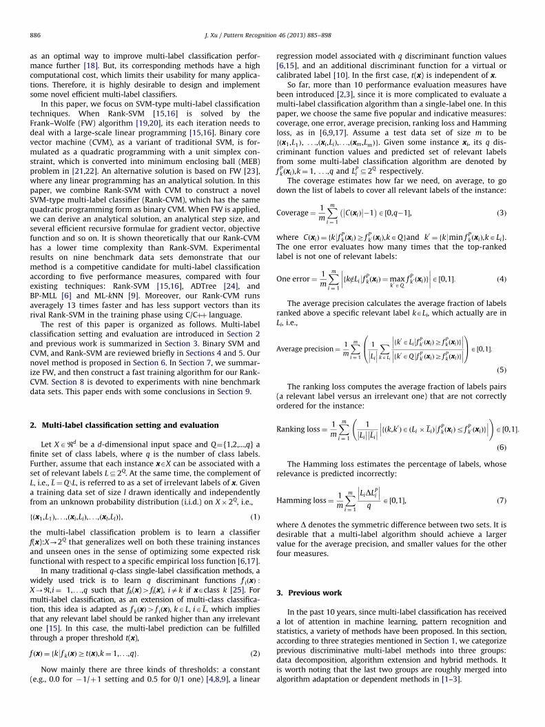
Pattern Recognition 46 (2013) 885–898
Contents lists available at SciVerse ScienceDirect
Pattern Recognition
0031-32
http://d
n Tel.:
E-m
journal homepage: www.elsevier.com/locate/pr
Fast multi-label core vector machine
Jianhua Xu n
School of Computer Science and Technology, Nanjing Normal University, Nanjing, Jiangsu 210097, China
a r t i c l e i n f o
Article history:
Received 28 November 2011
Received in revised form
6 June 2012
Accepted 3 September 2012Available online 11 September 2012
Keywords:
Support vector machine
Core vector machine
Multi-label classification
Frank–Wolfe method
Linear programming
Quadratic programming
03/$ - see front matter & 2012 Elsevier Ltd. A
x.doi.org/10.1016/j.patcog.2012.09.003
þ86 25 86306209; fax: þ86 25 85891990.
ail addresses: [email protected], xujianh
a b s t r a c t
The existing multi-label support vector machine (Rank-SVM) has an extremely high computational
complexity due to a large number of variables in its quadratic programming. When the Frank–Wolfe
(FW) method is applied, a large-scale linear programming still needs to be solved at any iteration.
Therefore it is highly desirable to design and implement a new efficient SVM-type multi-label
algorithm. Binary core vector machine (CVM), as a variant of traditional SVM, is formulated as a
quadratic programming with a unit simplex constraint, in which each linear programming in FW has an
analytical solution. In this paper, we combine Rank-SVM with CVM to construct a novel SVM-type
multi-label classifier (Rank-CVM) which is described as the same optimization form as binary CVM.
At its any iteration of FW, there exist analytical solution and step size, and several useful recursive
formulae for proxy solution, gradient vector, and objective function value, all of which reduce
computational cost greatly. Experimental study on nine benchmark data sets shows that when Rank-
CVM performs as statistically well as its rival Rank-SVM according to five performance measures, our
method runs averagely about 13 times faster and has less support vectors than Rank-SVM in the
training phase under C/Cþþ environment.
& 2012 Elsevier Ltd. All rights reserved.
1. Introduction
Multi-label classification is a special supervised learning issue, inwhich any single instance could be possibly associated with severalclasses simultaneously and thus the classes are no longer mutuallyexclusive [1–3]. Recently, it has been paid more attention to thanbefore due to lots of real-world applications, e.g., text categorization[4–7], scene and video annotation [8–11], bioinformatics [6,12,13],and music emotion categorization [14]. Currently, there are threemain strategies to design and implement various discriminativemulti-label classification methods: data decomposition, algorithmextension and hybrid strategies. Further, label correlation, i.e., labelco-occurrence information, has been exploited in four differentlevels: individual and partial instances, and pairwise and differentlabels.
Data decomposition strategy divides a multi-label data set intoeither one or more single-label (binary or multi-class) subsets,builds a sub-classifier for each subset using an existing classifier,and then assembles all sub-classifiers into an entire multi-labelclassifier. There are mainly three decomposition tricks: one-versus-rest (OVR), one-versus-one (OVO), and label powerset(LP) [1–3]. It is convenient to implement a data decompositionmulti-label method since lots of popular classifiers and their free
ll rights reserved.
software are available. This strategy depicts label correlation ofindividual instance, partial instances and pairwise labels respec-tively by reusing multi-label instances in the OVR methodsimplicitly, constructing possible label combinations in the LPmethods directly, and considering pairwise label combinationsin the OVO methods explicitly.
Algorithm extension strategy generalizes a specific multi-classclassification algorithm to consider all training instances and allclasses (or labels) of a multi-label training data set at once. Such astrategy could induce some complicated optimization problems,e.g., large-scale quadratic programming in multi-label supportvector machine (Rank-SVM) [15,16] and unconstrained optimiza-tion in multi-label back-propagation neural networks (BP-MLL) [6]. However, they explicitly characterize as many labelcorrelations of individual instance using pairwise constraintsbetween relevant labels and irrelevant ones as possible.
Hybrid strategy not only extends an existing single-labelmethod but also splits a multi-label data set into a series ofsubsets implicitly or explicitly. This strategy has been used todesign and implement several popular multi-label classifiers, e.g.,two kNN-based multi-label approaches (ML-kNN and IBLR-ML)[9,17], which cascade kNN with discrete Bayesian rule and logisticmodel respectively while the OVR trick is applied implicitly.Generally this strategy weakly characterizes label correlationseither explicitly or implicitly.
As mentioned above, algorithm extension strategy takes asmany label correlations into account as possible, which is regarded
J. Xu / Pattern Recognition 46 (2013) 885–898886
as an optimal way to improve multi-label classification perfor-mance further [18]. But, its corresponding methods have a highcomputational cost, which limits their usability for many applica-tions. Therefore, it is highly desirable to design and implementsome novel efficient multi-label classifiers.
In this paper, we focus on SVM-type multi-label classificationtechniques. When Rank-SVM [15,16] is solved by theFrank–Wolfe (FW) algorithm [19,20], its each iteration needs todeal with a large-scale linear programming [15,16]. Binary corevector machine (CVM), as a variant of traditional SVM, is for-mulated as a quadratic programming with a unit simplex con-straint, which is converted into minimum enclosing ball (MEB)problem in [21,22]. An alternative solution is based on FW [23],where any linear programming has an analytical solution. In thispaper, we combine Rank-SVM with CVM to construct a novelSVM-type multi-label classifier (Rank-CVM), which has the samequadratic programming form as binary CVM. When FW is applied,we can derive an analytical solution, an analytical step size, andseveral efficient recursive formulae for gradient vector, objectivefunction and so on. It is shown theoretically that our Rank-CVMhas a lower time complexity than Rank-SVM. Experimentalresults on nine benchmark data sets demonstrate that ourmethod is a competitive candidate for multi-label classificationaccording to five performance measures, compared with fourexisting techniques: Rank-SVM [15,16], ADTree [24], andBP-MLL [6] and ML-kNN [9]. Moreover, our Rank-CVM runsaveragely 13 times faster and has less support vectors than itsrival Rank-SVM in the training phase using C/Cþþ language.
The rest of this paper is organized as follows. Multi-labelclassification setting and evaluation are introduced in Section 2and previous work is summarized in Section 3. Binary SVM andCVM, and Rank-SVM are reviewed briefly in Sections 4 and 5. Ournovel method is proposed in Section 6. In Section 7, we summar-ize FW, and then construct a fast training algorithm for our Rank-CVM. Section 8 is devoted to experiments with nine benchmarkdata sets. This paper ends with some conclusions in Section 9.
1�:
2. Multi-label classification setting and evaluationLet XARd be a d-dimensional input space and Q¼{1,2,...,q} afinite set of class labels, where q is the number of class labels.Further, assume that each instance xAX can be associated with aset of relevant labels LD2Q. At the same time, the complement ofL, i.e., L¼Q \L, is referred to as a set of irrelevant labels of x. Givena training data set of size l drawn identically and independentlyfrom an unknown probability distribution (i.i.d.) on X�2Q, i.e.,
fðx1,L1Þ,. . .,ðxi,LiÞ,. . .,ðxl,LlÞg, ð1Þ
the multi-label classification problem is to learn a classifierf(x):X-2Q that generalizes well on both these training instancesand unseen ones in the sense of optimizing some expected riskfunctional with respect to a specific empirical loss function [6,17].
In many traditional q-class single-label classification methods, awidely used trick is to learn q discriminant functions f iðxÞ :X-R,i¼ 1,. . .,q such that fk(x)4fi(x), iak if xAclass k [25]. Formulti-label classification, as an extension of multi-class classifica-tion, this idea is adapted as f kðxÞ4 f iðxÞ, kAL, iAL, which impliesthat any relevant label should be ranked higher than any irrelevantone [15]. In this case, the multi-label prediction can be fulfilledthrough a proper threshold t(x),
f ðxÞ ¼ fk9f kðxÞZtðxÞ,k¼ 1,. . .,qg: ð2Þ
Now mainly there are three kinds of thresholds: a constant(e.g., 0.0 for �1/þ1 setting and 0.5 for 0/1 one) [4,8,9], a linear
regression model associated with q discriminant function values[6,15], and an additional discriminant function for a virtual orcalibrated label [10]. In the first case, t(x) is independent of x.
So far, more than 10 performance evaluation measures havebeen introduced [2,3], since it is more complicated to evaluate amulti-label classification algorithm than a single-label one. In thispaper, we choose the same five popular and indicative measures:coverage, one error, average precision, ranking loss and Hammingloss, as in [6,9,17]. Assume a test data set of size m to befðx1,L1Þ, . . .,ðxi,LiÞ,. . .,ðxm,LmÞg. Given some instance xi, its q dis-criminant function values and predicted set of relevant labelsfrom some multi-label classification algorithm are denoted byf P
kðxiÞ,k¼ 1, . . .,q and LPi D2Q respectively.
The coverage estimates how far we need, on average, to godown the list of labels to cover all relevant labels of the instance:
Coverage¼1
m
Xmi ¼ 1
CðxiÞ�� ���1� �
A ½0,q�1�, ð3Þ
where CðxiÞ ¼ fk9fPkðxiÞZ f P
k0 ðxiÞ,kAQgand k0 ¼ fk9min f PkðxiÞ,kALig.
The one error evaluates how many times that the top-rankedlabel is not one of relevant labels:
One error¼1
m
Xm
i ¼ 1
fk=2Li9fPkðxiÞ ¼max
k0AQf P
k0 ðxiÞg
��������A 0,1½ �: ð4Þ
The average precision calculates the average fraction of labelsranked above a specific relevant label kALi, which actually are inLi, i.e.,
Average precision¼1
m
Xm
i ¼ 1
1���Li
���XkALi
���fk0ALi
��f Pk0 ðxiÞZ f P
kðxiÞg
������fk0AQ��f P
k0 ðxiÞZ f PkðxiÞg
���0B@
1CAA 0,1½ �:
ð5Þ
The ranking loss computes the average fraction of labels pairs(a relevant label versus an irrelevant one) that are not correctlyordered for the instance:
Ranking loss¼1
m
Xm
i ¼ 1
1
Li
�� �� Li
�� �� fðk,k0ÞAðLi � LiÞ9fPkðxiÞr f P
k0 ðxiÞg
��� ��� !
A 0,½
ð6Þ
The Hamming loss estimates the percentage of labels, whoserelevance is predicted incorrectly:
Hamming loss¼1
m
Xmi ¼ 1
LiDLPi
��� ���q
A 0,1½ �, ð7Þ
where D denotes the symmetric difference between two sets. It isdesirable that a multi-label algorithm should achieve a largervalue for the average precision, and smaller values for the otherfour measures.
3. Previous work
In the past 10 years, since multi-label classification has receiveda lot of attention in machine learning, pattern recognition andstatistics, a variety of methods have been proposed. In this section,according to three strategies mentioned in Section 1, we categorizeprevious discriminative multi-label methods into three groups:data decomposition, algorithm extension and hybrid methods. Itis worth noting that the last two groups are roughly merged intoalgorithm adaptation or dependent methods in [1–3].
J. Xu / Pattern Recognition 46 (2013) 885–898 887
3.1. Data decomposition methods
Data decomposition methods combine data decompositiontricks with existing single-label classification methods, whose twokey techniques are decomposition tricks and integration ways.
The one-versus-rest (OVR) or binary relevance (BR) decom-position trick splits a q-class multi-label data set into q binarysubsets [4,8], in which the ith subset consists of positive instanceswith the ith label and negative ones with the all other labels.Usually, q sub-classifiers are assembled into an entire multi-labelalgorithm using a constant threshold. So far, many OVR multi-label methods have been verified to work well using variousbinary classifiers, e.g., SVM [1,4,8,15], C4.5 [1,17], and kNN [1,17].With a probabilistic output setting, the classification performancecan be improved further via a thresholding strategy [26].
The one-versus-one (OVO) decomposition trick divides aq-class multi-label data set into q(q�1)/2 binary subsets in apairwise way, where the subset ij (io j) only involves instanceswith the ith and jth labels. Note that for some subsets there is amixed class whose instances belong to both positive and negativeclasses simultaneously. In [27], these special subsets are handledby two binary SVM classifiers using the OVR strategy, and a votethreshold is used to detect relevant labels. But in [28], the mixedclasses are discarded simply. Further, a calibrated label is esti-mated by some OVR-based method, whose votes are defined as athreshold t(x) in (2). To reduce the test computational cost, threetwo-stage architectures are designed in [29].
The label powerset (LP) decomposition trick considers eachpossible label combination of more than one class as a new singleclass, and then converts a multi-label training set into a standardmulti-class one [1,8]. This could produce a large number of newclasses, many of which consist of very few instances. Such ashortcoming is avoided by LP-based ensemble classifiers in termsof a small subset of labels in [30].
3.2. Algorithm extension methods
Algorithm extension methods generalize existing multi-classclassifiers to consider all instances and all classes in a multi-labeldata set at once.
In [31], a C4.5-type multi-label algorithm was proposed,through modifying the formula of entropy calculation and per-mitting multiple labels at the leaves of the tree. BoosTexer [5] isderived from the well-known Adaboost algorithm, which includestwo slightly different versions: AdaBoost.MH and AdaBoost.MR.The former is to predict the set of relevant labels of an instance,while the latter to range labels of an instance in descending order.ADTree is constructed by integrating alternative decision treewith Adaboost.MH [24].
Multi-label support vector machine (Rank-SVM) was proposedin [15,16] via extending multi-class SVM [32] and accepting an
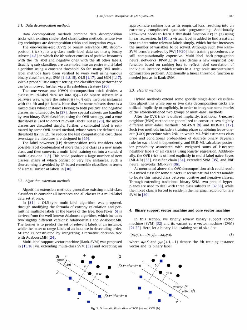
Fig. 1. Schematic illustration
approximate ranking loss as its empirical loss, resulting into anextremely complicated quadratic programming. AdditionallyRank-SVM needs to learn a threshold function t(x) in (2) usinglinear regression. In [10], a virtual label is added to find a naturalzero to determine relevant labels simply, which further increasesthe number of variables to be solved. Although such two Rank-SVM forms are solved by FW [19,20], their training procedures arestill computationally expensive. Multi-label back-propagationneural networks (BP-MLL) [6] also define a new empirical lossfunction based on ranking loss to reflect label correlation ofindividual instance, which results in a large scale unconstrainedoptimization problem. Additionally a linear threshold function isneeded just as in Rank-SVM.
3.3. Hybrid methods
Hybrid methods extend some specific single-label classifica-tion algorithms while one or two data decomposition tricks areutilized implicitly or explicitly, in order to integrate some meritsof the aforementioned two groups of multi-label methods.
After the OVR trick is utilized implicitly, traditional k-nearestneighbor (kNN) method are generalized to construct two slightlydifferent multi-label methods: ML-kNN [9] and IBLR-ML [17].Such two methods include a training phase combining leave-one-out (LOO) procedure with kNN, in which ML-kNN estimates classprior and conditional probabilities of discrete binary Bayesianrule for each label independently, and IBLR-ML calculates poster-ior probability associated with weighted sums of k-nearestneighbor labels of all classes using logistic regression. Addition-ally, the OVR trick is utilized explicitly in multi-label naıve Bayes(ML-NB) [33], classifier chain [34], extended SVM [35], and RBFneural networks (ML-RBF) [36].
As mentioned above, the OVO decomposition trick could resultin a mixed class for some subsets. It seems natural and reasonableto locate this mixed class between positive and negative classes.Through extending traditional binary SVM, two parallel hyper-planes are used to deal with three class subsets in [37,38], whilethe mixed class is forced to reside in the marginal region of binarySVM in [39].
4. Binary support vector machine and core vector machine
In this section, we briefly review binary support vectormachine (SVM) [32] and its variant core vector machine (CVM)[21,22]. Here, let a binary i.i.d. training set of size l be
fðx1,y1Þ,. . .,ðxi,yiÞ,. . .,ðxl,ylÞg, ð8Þ
where xiAX and yiA{þ1,�1} denote the ith training instancevector and its binary label.
of SVM (a) and CVM (b).
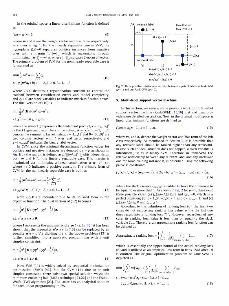
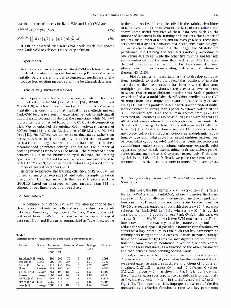
Fig. 2. Three possible relative relationships between a pair of labels in Rank-SVM
(r¼1) and our Rank-CVM (r40).
J. Xu / Pattern Recognition 46 (2013) 885–898888
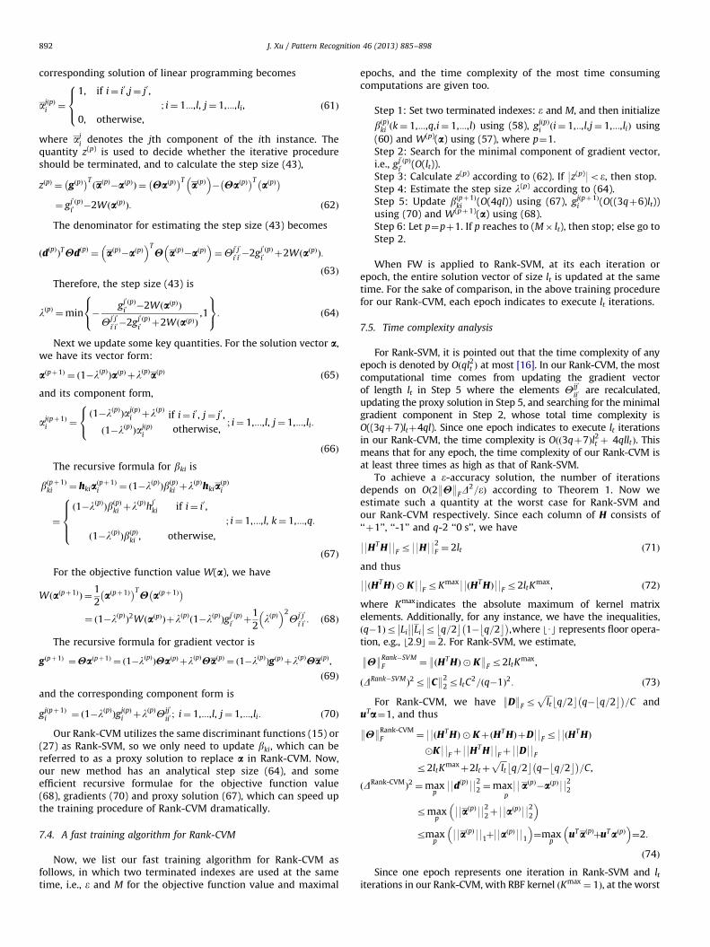
In the original space, a linear discriminant function is definedas
f ðxÞ ¼wT xþb, ð9Þ
where w and b are the weight vector and bias term respectively,as shown in Fig. 1. For the linearly separable case in SVM, thehyperplane f(x)¼0 separates positive instances from negativeones with a margin 1=99w992 which is maximizing throughminimizing 99w992
2 ¼wT w, where 99U992indicates 2-norm of vector.The primary problem of SVM for the nonlinearly separable case isformulated as
min1
2wT wþC
Xl
i ¼ 1
xi,
s:t: yi wT xiþb� �
Z1�xi,xiZ0, i¼ 1,. . .,l,
ð10Þ
where C40 denotes a regularization constant to control thetradeoff between classification errors and model complexity,and xiZ0 are slack variables to indicate misclassification errors.The dual version of (10) is
min1
2aT K � yyT� �
a�uTa,
s:t: yTa¼ 0,0rarCu, ð11Þ
where the symbol � represents the Hadamard product, a¼[a1,...,al]T
is the l Lagrangian multipliers to be solved, K ¼ xTi xj9i,j¼ 1,
�. . .,l �
denotes the symmetric kernel matrix, u¼[1,...,1]T and 0¼[0,...,0]T aretwo column vectors with l ones and zeros respectively, andy¼[y1,...,yl]
T indicates the binary label vector.In CVM, since the minimal discriminant function values for
positive and negative instances are denoted by 7r as shown inFig. 1(b), the margin is defined as r=99½wT ,b�T992which depends onboth w and b for the linearly separable case. This margin ismaximized via minimizing a linear combination wTwþb2
�nr,where n40 indicates a positive constant. The primary form ofCVM for the nonlinearly separable case is built as
min1
2ðwT wþb2
Þ�nrþ1
2CXl
i ¼ 1
x2i ,
s:t: yi wT xiþb� �
Zr�xi,rZ0, i¼ 1,. . .,l: ð12Þ
Note xiZ0 are redundant due to its squared form in theobjective function. The dual version of (12) becomes
min1
2aT K � yyTþyyTþ
1
CI
� �a,
s:t: uTaZn,aZ0, ð13Þ
where I represents the unit matrix of size l� l. In [40], it has beenshown that the inequality uTaZn in (13) can be replaced by anequality uTa¼n. Via dividing the n, the above problem (13) isfurther simplified into a quadratic programming with a unitsimplex constraint:
min1
2aT K � yyTþyyTþ
1
CI
� �a,
s:t: uTa¼ 1,aZ0: ð14Þ
Now SVM (11) is widely solved by sequential minimizationoptimization (SMO) [41]. But, for CVM (14), due to its unitsimplex constraint, there exist two special solution ways: theminimum enclosing ball (MEB) technique [21,22] and the Frank–Wolfe (FW) algorithm [23]. The latter has an analytical solutionfor each linear programming in FW.
5. Multi-label support vector machine
In this section, we review some previous work on multi-labelsupport vector machine (Rank-SVM) [15,16] first and then pro-vide more detailed description. Now, in the original input space, q
linear discriminant functions are defined as
f kðxÞ ¼wTk xþbk, k¼ 1,. . .,q, ð15Þ
where wk and bk denote the weight vector and bias term of the kthclass respectively. As mentioned in Section 2, it is desirable thatany relevant label should be ranked higher than any irrelevant.In case such an ideal situation does not happen, a slack variable isintroduced just as in binary SVM. Therefore, in Rank-SVM, therelative relationship between any relevant label and any irrelevantone for some training instance xi, is described using the followingpairwise constraint:
f mðxiÞ�f nðxiÞ ¼ ðwm�wnÞT xiþðbm�bnÞZ1�ximn, ðm,nÞA ðLi � LiÞ,
ð16Þ
where the slack variable ximnZ0 is added to force the difference tobe equal to or more than 1. As shown in Fig. 2 for r¼1, there existthree possible cases, (a) fm(xi)� fn(xi)Z1 and ximn¼0, which is aperfect situation; (b) 0ofm(xi)� fn(xi)o1 and 0oximno1; and (c)fm(xi)� fn(xi)r0 and ximnZ1.
According to the definition of ranking loss (6), the first twocases do not induce any ranking loss value, while the last onedoes result into a ranking loss ‘‘1’’. However, regardless of anycase, its ranking loss value is less than or equal to the slackvariable ximn. Therefore, an approximate ranking loss function canbe defined as
Approximate ranking loss¼1
l
Xl
i ¼ 1
1
Li
�� �� Li
�� �� Xðm,nÞA ðLi�LiÞ
ximn, ð17Þ
which is essentially the upper bound of the actual ranking loss(6) and is utilized as an empirical loss term in Rank-SVM after 1/lis omitted. The original optimization problem of Rank-SVM isdepicted as
min1
2
Xq
k ¼ 1
wTk wkþC
Xl
i ¼ 1
1
Li
�� �� Li
�� �� Xðm,nÞA ðLi�LiÞ
ximn,
s:t: ðwm�wnÞT xiþðbm�bnÞZ1�ximn,
ximnZ0,ðm,nÞAðLi � LiÞ,i¼ 1,. . .,l: ð18Þ
J. Xu / Pattern Recognition 46 (2013) 885–898 889
The model regularization term, i.e., the first one in the aboveobjective function, is defined according to the corresponding termin binary SVM. Using the standard Lagrangian technique, the dualversion of (18) is derived as follows [15,16]:
min1
2
Xq
k ¼ 1
Xl
i,j ¼ 1
bkibkjðxTi xjÞ�
Xl
i ¼ 1
Xðm,nÞA ðLi�LiÞ
aimn,
s:t:Xl
i ¼ 1
Xðm,nÞA ðLi�LiÞ
ckimnaimn ¼ 0, k¼ 1,:::,q,
0raimnrCi ¼1
Li
�� �� Li
�� ��C,ðm,nÞAðLi � LiÞ, i¼ 1,. . .,l, ð19Þ
with
ckimn ¼
0
þ1
�1
if mak and nak,
if m¼ k,
if n¼ k,
8><>: ð20Þ
and
bki ¼X
ðm,nÞA ðLi�LiÞ
ckimnaimn: ð21Þ
In [15,16], the above component-based form is described only.Now we transform (19) and (21) into concise vector and matrixrepresentations. For the ith instance, we construct a column vectorai with aimn, a row vector hki with ck
imn and a unit vector ui, whoselength is li ¼ 9Li99Li9, and a matrix Hi of size q� li using hki
ai ¼ aimn9ðm,nÞAðLi � LiÞ� �T
¼ aji9j¼ 1,. . .,li
h iT,
hki ¼ ckimn9ðm,nÞA ðLi � LiÞ
h i¼ hj
ki9j¼ 1,. . .,lih i
,
ui ¼ 1,. . .,1½ �T ,
Hi ¼ hT1i,. . .,h
Tqi
h iT: ð22Þ
According to (22), the formulae (21) and (19) can be simplified as
bki ¼ hkiai, ð23Þ
and
min1
2
Xm
i,j ¼ 1
aTi ðH
Ti HjÞajðx
Ti xj�
Xl
i ¼ 1
uTi ai,
s:t:Xl
i ¼ 1
Hiai ¼ 0,0rairCiui, ð24Þ
Further, using (22), we define a solution vector a and a unitvector u, whose length is lt ¼
Pli ¼ 1 li, and a new matrix H of size
q� lt and a kernel matrix K of size lt� lt
a¼ aT1,. . .,aT
i ,. . .,aTl
� �T,
u¼ uT1 ,. . .,uT
l
� �T,
H ¼ H1,. . .,Hi,. . .,Hl½ �,
K ¼ ðxTi xjÞðuiu
Tj Þ9i,j¼ 1,. . .,l
h i: ð25Þ
In terms of (25), the above quadratic programming (24) can berewritten as a more concise form:
min WðaÞ ¼1
2aT ðHT HÞ � K
a�uTa,
s:t: Ha¼ 0,0rarC, ð26Þ
where the column vector C ¼ C1uT1 . . . Clu
Tl
h iT. Due to lt vari-
ables to be solved, this quadratic programming (26) has anextremely high computational complexity. Now, the above Rank-SVM (19) or (26) is solved by the FW method [19], where anyiteration needs to solve a large-scale linear programming [16].
Similarly in binary SVM and CVM [21,22,32], the dot productbetween two vectors in (25) can be replaced by various kernels [32],and q nonlinear discriminant functions with kernel are rewritten as
f kðxÞ ¼Xl
i ¼ 1
bkiKðx,xiÞþbk,k¼ 1,. . .,q, ð27Þ
where K(x,xi) denotes some kernel function [32]. To determine thethreshold function t(x) in (2), each training instance xi is convertedinto a q-dimensional vector [f1(xi),....,fq(xi)]
T using (27), and then anoptimal threshold t*(xi) is determined via minimizing the Hammingloss (7). A linear regression threshold function is trained in Rank-SVM, i.e., tðxÞ ¼
Pqk ¼ 1 skf kðxÞþs0, where si(i¼0,1,...,q) represent the
regression coefficients. Then this threshold form is used to predictthe relevant labels in the test phase.
6. Multi-label core vector machine
In this section, we combines Rank-SVM with binary CVM toconstruct a novel multi-label SVM-type classifier (Rank-CVMsimply), whose any iteration of FW has an analytical solution.
Now it is still desired that any relevant label should be rankedhigher than any irrelevant one. According to the constraints inbinary CVM and Rank-SVM, we define the following pairwiseconstraints for Rank-CVM:
f mðxiÞ�f nðxiÞ ¼ ðwm�wnÞT xiþðbm�bnÞZr�ximn,ðm,nÞAðLi � LiÞ,
ð28Þ
where the slack variable ximn is used to force the difference to bemore than r40. As shown in Fig. 2 for r40, there still are threepossible situations: (a) fm(xi)� fn(xi)Zr and ximn¼0; (b) 0o fm(xi)� fn(xi)or and 0oximnor; and (c) fm(xi)� fn(xi)r0 and ximnZr.According to the ranking loss (6), it could be found out that theranking loss value is always less than or equal to ximn/r. There-fore, an approximate ranking loss function for Rank-CVM can bedefined as follows:
Approximate ranking loss¼1
lr2
Xl
i ¼ 1
1
Li
�� �� Li
�� �� Xðm,nÞA ðLi�LiÞ
x2imn: ð29Þ
This is used as an empirical loss term when1/lr2 is removed inour Rank-CVM. On the other hand, we constitute a modelregularization term ð1=2Þ
Pqk ¼ 1ðw
Tk wkþb2
k Þ�nr for Rank-CVM interms of binary CVM and Rank-SVM principles. Now we formu-late the primary form of our Rank-CVM as
min1
2
Xq
k ¼ 1
ðwTk wkþb2
k Þ�nrþ1
2CXl
i ¼ 1
1
Li
�� �� Li
�� �� Xðm,nÞA ðLi�LiÞ
x2imn,
s:t: ðwm-wnÞT xiþðbm-bnÞ ¼
Xq
k ¼ 1ck
imnðwTk xiþbkÞZr�ximn,
r40,ðm,nÞAðLi � LiÞ,i¼ 1,:::,l: ð30Þ
Note that ximnZ0 hold naturally due to the squared form ofslack variables in the objective function (30), and the conciseconstraints are reformulated according to the definition of ck
imnin(20). Again, C represents the regularization constant to control thetradeoff between the model complexity and the ranking loss.
The dual problem of (30) can be derived using the standardLagrangian technique. Let aimnZ0 and ZZ0 be the Lagrangianmultipliers for the inequality constraints in (30). The Lagrangianfor the primal form (30) becomes
L¼1
2
Xq
k ¼ 1
ðwTk wkþb2
k Þ�nrþ1
2
Xl
i ¼ 1
Ci
Xðm,nÞA ðLi�LiÞ
x2imn
�Xl
i ¼ 1
Xðm,nÞA ðLi�LiÞ
aimn
Xq
k ¼ 1
ckimn wk
T xiþbk
� ��rþximn
!�Zr, ð31Þ

J. Xu / Pattern Recognition 46 (2013) 885–898890
where Ci ¼ C= Li
�� �� Li
�� ��. The Karush–Kuhn–Tucker (KKT) conditionsfor this primary problem require the following relations to be true
@L
@wk¼ 0) wk ¼
Xl
i ¼ 1
Xðm,nÞA ðLi�LiÞ
ckimnaimn
0@
1Axi ¼
Xl
i ¼ 1
bkixi, ð32Þ
@L
@bk¼ 0) bk ¼
Xl
i ¼ 1
Xðm,nÞA ðLi�LiÞ
ckimnaimn ¼
Xl
i ¼ 1
bki, ð33Þ
@L
@r¼ 0)
Xl
i ¼ 1
Xðm,nÞA ðLi�LiÞ
aimn ¼ nþZ, ð34Þ
@L
@ximn¼ 0) aimn ¼ Ciximn: ð35Þ
The last relation (35) shows that ximnZ0 hold naturally due toaimnZ0. By introducing the above KKT conditions (32)-(35) intothe Lagrangian (31), the dual form is
min WðaÞ ¼1
2
Xq
k ¼ 1
Xl
i,j ¼ 1
bkibkjðxTi xjÞþ
1
2
Xq
k ¼ 1
Xl
i,j ¼ 1
bkibkj
þ1
2
Xl
i ¼ 1
1
Ci
Xðm,nÞA ðLi�LiÞ
a2imn
0@
1A,
s:t:Xl
i ¼ 1
Xðm,nÞA ðLi�LiÞ
aimnZn;aimnZ0,ðm,nÞA ðLi � LiÞ, i¼ 1,:::,l: ð36Þ
According to those notions in (22) and (25), and the derivationof binary CVM, this formula (36) can further be simplified into aquadratic programming with a unit simplex constraint too
min WðaÞ ¼1
2
Xl
i,j ¼ 1
Xq
k ¼ 1
aTi ðh
TkihkjÞaj
!ðxT
i xjÞ
þ1
2
Xl
i,j ¼ 1
Xq
k ¼ 1
aTi ðh
TkihkjÞaj
!þ
1
2
Xl
i ¼ 1
1
CiaT
i ai
� �
¼1
2
Xl
i,j ¼ 1
aTi ðH
Ti HjÞajðx
Ti xjÞþ
1
2
Xl
i,j ¼ 1
aTi ðH
Ti HjÞajþ
1
2
Xl
i ¼ 1
1
CiaT
i ai
� �
¼1
2aT ðHT HÞ � KþHT HþD
a¼1
2aTHa,
s:t: uTa¼ 1, aZ0, ð37Þ
where
D¼ diagðuT1=C1,::::,uT
l =ClÞ,
H¼ ðHT HÞ � KþðHT HÞþD: ð38Þ
Similarly, our Rank-CVM (37) and its q discriminant functions(15) can also be kernelized by various kernels satisfying Mercertheorem [32]. Additionally, Rank-CVM also needs a thresholdfunction, which is estimated using the same method as in Rank-SVM. Although our Rank-CVM (37) has the same number ofvariables to be solved as Rank-SVM (26), due to a unit simplexconstraint in (37), we can construct a fast training algorithmbased on FW for our Rank-CVM.
7. A fast training algorithm for Rank-CVM
In this section, a fast training algorithm for our Rank-CVM isconstructed based on the Frank–Wolfe iterative linearizationalgorithm.
7.1. Frank–Wolfe algorithm
In this sub-section we briefly review the Frank–Wolfe (FW)method and its three special cases, from which both Rank-SVM
and Rank-CVM will benefit a lot. FW is a simple and classical firstorder feasible direction optimization method [19], which wasoriginally proposed to solve quadratic programming and thenextended to solve convex problems with continuously differentialobjective function and linear (and box) constraints:
min f ðxÞ, s:t:xAS: ð39Þ
The set S is a nonempty and bounded polyhedron of the form,
S¼ fx9Ax¼ b,lrxrug, ð40Þ
where A is a m�n matrix, b represents a m-dimensional columnvector, and l and u denote the lower and upper bounds of x. FWgenerates a sequence of feasible vectors {x(p)} using a linear
search x(pþ1)¼x(p)
þl(p)d(p), where l(p)A[0,1] is a step size and
dðpÞ ¼ xðpÞ� xðpÞ a feasible descent direction satisfying xðpÞAS and
z(p)¼(d(p))Trf(x(p))o0. To find out a best feasible direction, i.e.,
the best xðpÞ, FW utilizes the first order Taylor series expansion off(x) around the vector x(p) and then solves a linear programmingproblem with linear constraints (40):
xðpÞ ¼ argminxA S
f ðxðpÞÞþðx�xðpÞÞTrf ðxðpÞÞ
¼ argminxA S
xTrf ðxðpÞÞ:
ð41Þ
Such a linear programming problem is usually optimized bythe widely used simplex or interior point method. The basic FWalgorithm for (39) can be stated as follows:
Step 1 (initializing): Select an initial feasible vector x(p)AS withp¼1 and set a stop criterion e.Step 2 (solving a linear programming problem): LetxðpÞ ¼ argmin
xASxTrf ðxðpÞÞ. If 9z(p)9re, then stop.
Step 3 (executing a linear search for step size): Let lðpÞ ¼argminlA ½0,1�
f ðxðpÞ þlðxðpÞ�xðpÞÞÞ.
Step 4 (updating): Set xðpþ1Þ ¼ xðpÞ þlðpÞðxðpÞ�xðpÞÞ and p¼pþ1,go to Step 2.
It was proved that the above FW algorithm has a sub-linearconvergence [19,20]. We rewrite the objective functions in Rank-SVM and our Rank-CVM into a unified concise quadratic form:
f ðxÞ ¼1
2xTHxþhT x, ð42Þ
where H¼ ðHT HÞ � K and h¼u in Rank-SVM, and H¼ ðHT HÞ�KþðHT HÞþD and h¼0 in Rank-CVM. For some widely usedMercer kernels, e.g., linear, polynomial and RBF kernels, such anobjective function (42) is strictly convex generally [32]. To speedup the training procedures of Rank-SVM and our Rank-CVM, threespecial cases can be exploited, i.e.,
Case 1. For the strictly convex objective function (42), theanalytical step size of FW becomes
lðpÞ ¼min �zðpÞ
ðdðpÞÞTHdðpÞ,1
( ): ð43Þ
This formula can be used to estimate the step size for Rank-SVM and our Rank-CVM efficiently.
Case 2. If the strictly convex function f(x) in (42) has an optimalvalue fn, and {x(p)} and {z(p)} are derived by FW (p¼1,2..., x(1)AS), then,
f ðxðpÞÞ�f nr�zðpÞ ¼ �ðHxðpÞ þhÞT dðpÞ: ð44Þ
Therefore, when 9z(p)9re, we have f(x(p))� f*re. This impliesthat, when the stopping criterion e is satisfied in Step 2 thedifference between the current function value and the optimalone is less than e.
J. Xu / Pattern Recognition 46 (2013) 885–898 891
Case 3. For a unit simplex constraint in our Rank-CVM, the linearprogramming in Step 3 is
minXn
i ¼ 1
HxðpÞ� �
ixðpÞi , s:t:
Xn
i ¼ 1
xðpÞi ¼ 1, ð45Þ
where (Hx(p))i denotes the ith component of gradient vector.Then, the above (45) has an analytical solution:
xðpÞj ¼1
0
if j¼ argmini ¼ 1,:::,n
HxðpÞ� �
i,
otherwise:
8<: ð46Þ
That is, the component with a minimum derivate is 1, and theother components all are 0. Therefore, we can obtain an analyticalsolution directly for our Rank-CVM, which greatly reduces thecomputational time of the training procedure.
To decide how many iterations are theoretically needed to solveRank-SVM and our Rank-CVM, we provide the rate of convergenceof FW for (42) using the following theorem 1, in which we utilizesome techniques in [19,20,23].
Theorem 1. Let x* be optimal for the quadratic programming (42)with the feasible set S (40), and {x(p)} a sequence generated byFW. Then there exists a constant xZ�1 such that
f ðxðpÞÞ�f ðxnÞr2:H:FD
2
pþx, ð47Þ
where :H:F indicates Frobenius norm of matrix, and D is thediameter of S.
Proof. According to x(pþ1)¼x(p)
þl(p)d(p) and the step size l(p) in(43), we have
f ðxðpþ1ÞÞ ¼1
2xðpÞ þlðpÞdðpÞ T
H xðpÞ þlðpÞdðpÞ
þhT xðpÞ þlðpÞdðpÞ
¼ f ðxðpÞÞ�1
2
ðHxðpÞ þhÞT dðpÞ 2
ðdðpÞÞTHdðpÞ: ð48Þ
Using (44), the above (48) can be rewritten as
f ðxðpþ1ÞÞ�f ðxnÞr f ðxðpÞÞ�f ðxnÞ�1
2
f ðxðpÞÞ�f ðxnÞ� �2
ðdðpÞÞTHdðpÞ: ð49Þ
Set dðpÞ ¼ 2ðdðpÞÞTHdðpÞr2:H:F:dðpÞ:2
2r2:H:FD2¼ d, where
D¼max99p
dðpÞ992, namely, the diameter of S. Since (1�a)(1þa)¼
1�a2r1 if aZ0, the inequality holds: 1�ar1/(1þa).Denoting b(p)
¼ f(x(p))� f(x*)Z0, it follows that
bðpþ1ÞrbðpÞ�ðbðpÞÞ2
dðpÞr
bðpÞ
1þbðpÞ=dðpÞ¼
1
1=bðpÞ þ1=dðpÞr
1
1=bðpÞ þ1=dð50Þ
For k¼1, its step size l(1)¼�(Hx(1)
þh)Td(1)/d(1)r1 andaccording to (44), we have b(1)rl(1)d(1)rl(1)d.
By inducing, we derive the following inequalities:
bð2Þr1
1=dþ1=lð1Þd¼
d1þ1=lð1Þ
, bð3Þr1
1=dþ1=bð2Þ¼
d2þ1=lð1Þ
. . .,
bðpÞr ¼d
p�1þ1=lð1Þ: ð51Þ
Since 0rl(1)r1, let x¼1/l1�1Z�1, and then we have
f ðxðpÞÞ�f ðxnÞrd
pþx¼
2:H:FD2
pþx, ð52Þ
which completes our proof. This theorem implies that, to achievea e-accuracy solution, i.e., e¼ f(x(p))� f(x*), FW needsOð2:H:FD
2=eÞ iterations for a convex quadratic programming(42). &
7.2. Initialization for training algorithm of Rank-CVM
In order to apply the above FW method to our Rank-CVM, wehave to initialize a solution vector and some other key quantities.According to (38), the elements in the matrix H are
Yjj0
ii0¼Xq
k ¼ 1
hjkih
j0
ki0ðxT
i xi0 þ1Þþ1
Cidjj0
ii0; i,i0 ¼ 1,:::,l, j¼ 1,:::,li, j0 ¼ 1,:::,li0 ,
ð53Þ
where djj0
ii0¼ 1, if i¼ i’, j¼ j’ and djj0
ii0¼ 0 otherwise. This element in
(53) corresponds to the jth row of the ith instance and the j’thcolumn of the i’th instance. But, the diagonal elements only have l
different values,
Yjjii ¼ 2 ðxT
i xiÞþ1� �
þ1
Ci; i¼ 1,:::,l and any j: ð54Þ
We search for the i’th instance which minimize the above (54), i.e.,
i0 ¼ argmini ¼ 1,:::,l
Yjjii: ð55Þ
Therefore, according to the unit simplex constraint, we choosean initial solution as
ajð1Þi ¼
1, if i¼ i0,j¼ 1,
; i¼ 1,:::,l, j¼ 1,:::,li,
0, otherwise,
8><>: ð56Þ
where the superscript (1) indicates the initial solution. In (56), thefirst component of the i’th instance is set to be 1 only. In this case,the initial objective function value is
W ð1ÞðaÞ ¼ ðxT
i xiÞþ1� �
þ1
2Ci0ð57Þ
and the initial bð1Þki becomes
bð1Þki ¼h1
ki
0
if i¼ i0,
otherwise,; i¼ 1,:::,l, k¼ 1,:::,q,
(ð58Þ
where h1ki denotes the first element of the row vector hki. This
indicates that the initial bð1Þki0ðk¼ 1,:::,qÞ are set to be the first
column vector of Hi’. The gradient vector of the objective functionin (37) is
gi ¼Xl
j ¼ 1
Xq
k ¼ 1
ðhTkihkjÞaj ðx
Ti xjÞþ1
� �þ
1
Ciai,or g ¼Ha: ð59Þ
where gi corresponds to ai of the ith instance, andg ¼ gT
1 ::: gTl
h iT. Therefore the initial gradients are
gjð1Þi ¼
Xq
k ¼ 1
hjkih
1ki0 ðx
Ti xi0 Þþ1
� �þ
1
Ciif i¼ i0,j¼ 1,
; i¼ 1,:::,l,j¼ 1,:::,li:Xq
k ¼ 1
hjkih
1ki0 ðx
Ti xi0 Þþ1
� �otherwise,
8>>>>>>><>>>>>>>:
ð60Þ
7.3. Some useful recursive formulae for training algorithm of Rank-
CVM
After the above quantities have been initialized, we derivesome useful recursive formulae in this sub-section. At the pth(p¼1, 2,y) iteration, assume the minimum gradient componentto be gj0 ðpÞ
i0. According to the special case 3 in Section 7.1, the
J. Xu / Pattern Recognition 46 (2013) 885–898892
corresponding solution of linear programming becomes
ajðpÞi ¼
1, if i¼ i0,j¼ j0,
; i¼ 1:::,l, j¼ 1,:::,li,
0, otherwise,
8><>: ð61Þ
where aji denotes the jth component of the ith instance. The
quantity z(p) is used to decide whether the iterative procedureshould be terminated, and to calculate the step size (43),
zðpÞ ¼ gðpÞ� �T
ðaðpÞ�aðpÞÞ ¼ HaðpÞ� �T
aðpÞ
� HaðpÞ� �T
aðpÞ� �
¼ gj0 ðpÞi0�2WðaðpÞÞ: ð62Þ
The denominator for estimating the step size (43) becomes
ðdðpÞÞTHdðpÞ ¼ aðpÞ�aðpÞ T
H aðpÞ�aðpÞ
¼Yj0 j0
i0 i0�2gj0 ðpÞ
i0þ2WðaðpÞÞ:
ð63Þ
Therefore, the step size (43) is
lðpÞ ¼min �gj0 ðpÞ
i0�2WðaðpÞÞ
Yj0 j0
i0 i0�2gj0 ðpÞ
i0þ2WðaðpÞÞ
,1
8<:
9=;: ð64Þ
Next we update some key quantities. For the solution vector a,we have its vector form:
aðpþ1Þ ¼ ð1�lðpÞÞaðpÞ þlðpÞaðpÞ ð65Þ
and its component form,
ajðpþ1Þi ¼
ð1�lðpÞÞajðpÞi þl
ðpÞ
ð1�lðpÞÞajðpÞi
if i¼ i0, j¼ j0,
otherwise,; i¼ 1,:::,l, j¼ 1,:::,li:
8<:
ð66Þ
The recursive formula for bki is
bðpþ1Þki ¼ hkia
ðpþ1Þi ¼ ð1�lðpÞÞbðpÞki þl
ðpÞhkiaðpÞi
¼
ð1�lðpÞÞbðpÞki þlðpÞhj0
ki if i¼ i0,
; i¼ 1,:::,l, k¼ 1,:::,q:
ð1�lðpÞÞbðpÞki , otherwise,
8>><>>:
ð67Þ
For the objective function value W(a), we have
Wðaðpþ1ÞÞ ¼1
2aðpþ1Þ� �T
H aðpþ1Þ� �
¼ ð1�lðpÞÞ2WðaðpÞÞþlðpÞð1�lðpÞÞgj0 ðpÞi0þ
1
2lðpÞ 2
Yj0j0
i0i0: ð68Þ
The recursive formula for gradient vector is
gðpþ1Þ ¼Haðpþ1Þ ¼ ð1�lðpÞÞHaðpÞ þlðpÞHaðpÞ ¼ ð1�lðpÞÞgðpÞ þlðpÞHaðpÞ,
ð69Þ
and the corresponding component form is
gjðpþ1Þi ¼ ð1�lðpÞÞgjðpÞ
i þlðpÞYjj0
ii0; i¼ 1,:::,l, j¼ 1,:::,li: ð70Þ
Our Rank-CVM utilizes the same discriminant functions (15) or(27) as Rank-SVM, so we only need to update bki, which can bereferred to as a proxy solution to replace a in Rank-CVM. Now,our new method has an analytical step size (64), and someefficient recursive formulae for the objective function value(68), gradients (70) and proxy solution (67), which can speed upthe training procedure of Rank-CVM dramatically.
7.4. A fast training algorithm for Rank-CVM
Now, we list our fast training algorithm for Rank-CVM asfollows, in which two terminated indexes are used at the sametime, i.e., e and M for the objective function value and maximal
epochs, and the time complexity of the most time consumingcomputations are given too.
Step 1: Set two terminated indexes: e and M, and then initialize
bðpÞki ðk¼ 1,:::,q,i¼ 1,:::,lÞ using (58), gjðpÞi ði¼ 1,::,l,j¼ 1,:::,liÞ using
(60) and W(p)(a) using (57), where p¼1.Step 2: Search for the minimal component of gradient vector,i.e., gj0 ðpÞ
i0(O(lt)).
Step 3: Calculate z(p) according to (62). If 9z(p)9oe, then stop.Step 4: Estimate the step size l(p) according to (64).Step 5: Update bðpþ1Þ
ki (O(4ql)) using (67), gjðpþ1Þi (O((3qþ6)lt))
using (70) and W(pþ1)(a) using (68).Step 6: Let p¼pþ1. If p reaches to (M� lt), then stop; else go toStep 2.
When FW is applied to Rank-SVM, at its each iteration orepoch, the entire solution vector of size lt is updated at the sametime. For the sake of comparison, in the above training procedurefor our Rank-CVM, each epoch indicates to execute lt iterations.
7.5. Time complexity analysis
For Rank-SVM, it is pointed out that the time complexity of anyepoch is denoted by Oðql2t Þ at most [16]. In our Rank-CVM, the mostcomputational time comes from updating the gradient vectorof length lt in Step 5 where the elements Yjj0
ii0are recalculated,
updating the proxy solution in Step 5, and searching for the minimalgradient component in Step 2, whose total time complexity isO((3qþ7)ltþ4ql). Since one epoch indicates to execute lt iterationsin our Rank-CVM, the time complexity is Oðð3qþ7Þl2t þ 4qlltÞ. Thismeans that for any epoch, the time complexity of our Rank-CVM isat least three times as high as that of Rank-SVM.
To achieve a e-accuracy solution, the number of iterationsdepends on Oð2:H:FD
2=eÞ according to Theorem 1. Now weestimate such a quantity at the worst case for Rank-SVM andour Rank-CVM respectively. Since each column of H consists of‘‘þ1’’, ‘‘-1’’ and q-2 ‘‘0 s’’, we have
99HT H99F r99H992
F ¼ 2lt ð71Þ
and thus
99ðHT HÞ � K99F rKmax99ðHT HÞ99F r2ltKmax, ð72Þ
where Kmaxindicates the absolute maximum of kernel matrixelements. Additionally, for any instance, we have the inequalities,ðq�1Þr Li
�� �� Li
�� ��r q=2� �
1� q=2� �� �
,where Ub c represents floor opera-tion, e.g., 2:9b c ¼ 2. For Rank-SVM, we estimate,
:H:Rank�SVM
F ¼ :ðHT HÞ � K:F r2ltKmax,
ðDRank�SVMÞ2r:C:2
2r ltC2=ðq�1Þ2: ð73Þ
For Rank-CVM, we have :D:F rffiffiffilt
pq=2� �
q� q=2� �� �
=C anduTa¼1, and thus
:H:Rank-CVM
F ¼ 99ðHT HÞ � KþðHT HÞþD99F r99ðHT HÞ
�K99Fþ99HT H99Fþ99D99F
r2ltKmaxþ2ltþ
ffiffiffilt
pq=2� �
q� q=2� �� �
=C,
ðDRank-CVMÞ2¼max
p99dðpÞ992
2 ¼max99p
aðpÞ�aðpÞ992
2
rmaxp
99aðpÞ992
2þ99aðpÞ992
2
rmax
p99aðpÞ991þ99a
ðpÞ991
¼max
puTaðpÞþuTaðpÞ
¼2:
ð74Þ
Since one epoch represents one iteration in Rank-SVM and ltiterations in our Rank-CVM, with RBF kernel ðKmax
¼ 1Þ, at the worst
J. Xu / Pattern Recognition 46 (2013) 885–898 893
case the number of epochs for Rank-SVM and Rank-CVM are
ORank-SVMð4l2t C2=ðq�1Þ2=eÞ, ð75Þ
ORank-CVM 16þ4 q=2� �
q� q=2� �� �
=Cffiffiffilt
ph i=e
: ð76Þ
It can be observed that Rank-CVM needs much less epochsthan Rank-SVM to achieve a e-accuracy solution.
8. Experiments
In this section, we compare our Rank-CVM with four existingmulti-label classification approaches including Rank-SVM experi-mentally. Before presenting our experimental results, we brieflyintroduce four existing methods and nine benchmark data sets.
8.1. Four existing multi-label methods
In this paper, we selected four existing multi-label classifica-tion methods: Rank-SVM [15], ADTree [24], BP-MLL [6] andML-kNN [9], which will be compared with our Rank-CVM experi-mentally. It is worth noting that the first three methods and ourRank-CVM belong to algorithm extension methods considering alltraining instances and all labels at the same time, while ML-kNNis a typical hybrid method based on the OVR data decompositiontrick. We downloaded the original C/Cþþ software package ofADTree from [42] and the Matlab ones of BP-MLL and ML-kNNfrom [43]. For ADTree, we utilize its original name rather thanADTBoost.MR in [6,9], and slightly modified its software tocalculate the ranking loss. On the other hand, we accept theirrecommended parameter settings. For ADTree, the number ofboosting rounds is set to be 50. For BP-MLL, the number of hiddenneurons is 20% of the number of input neurons, the trainingepochs is set to be 100 and the regularization constant is fixed tobe 0.1. For ML-kNN, the Laplacian estimator (s¼1) is used and thenumber of nearest instances k¼10.
In order to improve the training efficiency of Rank-SVM, weutilized an analytical step size (64) and coded its implementationusing C/Cþþ language, in which the free C language packageLPSOL5.5 based on improved simplex method from [44] isadopted as our linear programming solver.
8.2. Nine data sets
To compare our Rank-CVM with the aforementioned fourclassification methods, we collected seven existing benchmarkdata sets: Emotions, Image, Scene, Genbase, Medical, Slashdot,and Yeast from [43,45,46], and constructed two new biologicaldata sets: Plant and Human, as summarized in Table 1, according
Table 1Statistics for nine benchmark data sets used in our experiments.
Data set Domain Instances Features Classes Average
labels
Variables
Train Test
Emotions[45] Music 391 202 72 6 1.87 2793
Image[43] Scene 1200 800 294 5 1.24 5342
Scene[45] Scene 1211 1196 294 6 1.07 6278
Plant Biology 588 390 440 12 1.08 6959
Genbase[45] Biology 463 199 1185 27 1.35 14808
Human Biology 1862 1244 440 14 1.19 28036
Medical[45] Text 645 333 1449 45 1.25 34878
Slashdot[46] Text 2269 1513 1079 22 1.18 55306
Yeast[45] Biology 1500 917 103 14 4.24 58248
to the number of variables to be solved in the training algorithmsof Rank-CVM and our Rank-SVM in the last column. Table 1 alsoshows some useful statistics of these data sets, such as, thenumber of instances in the training and test sets, the number offeatures, the number of labels, and the average labels. These datasets cover four distinct domains: text, scene, music and biology.
For seven existing data sets, the Image and Slashdot arepartitioned into training and test sets randomly according to60% versus 40% by us, while the other five training and test setsare downloaded directly from their web sites [45]. For moredetailed information and description for these seven data sets,please refer to their corresponding web sites and referencestherein [43,45,46].
In bioinformatics, an important task is to develop computa-tional methods to predict the subcellular locations of proteinsaccording to their sequences. It has been observed that somemultiplex proteins can simultaneously exist at two, or movebetween, two or more different location sites. Such a problemwas identified as a multi-label classification, handled by the OVRdecomposition trick simply, and evaluated by accuracy of eachclass [13]. But, this problem is dealt with under standard multi-label classification setting in this paper. We downloaded 978 and3106 sequences for Plant and Human species from [47], andextracted 440 features (20 amino acid, 20 pseudo-amino acid and400 dipetide compositions) from each protein sequence under thedefault setting using the free off-line software PseAAC-Builderfrom [48]. The Plant and Human include 12 location sites (cellmembrace, cell wall, chloroplast, cytoplasm, endoplasmic reticu-lum, extracellular, golgi apparatus, mitochondrion, nucleus, per-oxisome, plastid, and vacuole), and 14 ones (centriole, cytoplasm,cytoskeleton, endoplasm reticulum, endosome, extracell, golgi,apparatus, lysosome, microsome, mitochondrion, nucleus, peroxi-some, plasma membrace, and synapse) respectively. Their aver-age labels are 1.08 and 1.19. Finally we parse these two sets intotraining and test data sets randomly in terms of 60% versus 40%.
8.3. Tuning two key parameters for Rank-CVM and Rank-SVM on
training sets
In this work, the RBF kernel Kðx,yÞ ¼ expð�g:x�y:2
2Þ is testedfor Rank-SVM and our Rank-CVM, where g denotes the kernelscale factor. Additionally, such two methods involve a regulariza-tion constant C. To reach an acceptable classification performance,M¼50 are recommended without achieving a e¼10�3 accuracysolution for Rank-SVM in [6,9], whereas e¼10�3 is quicklysatisfied within 1–2 epochs for our Rank-CVM. In this case, weset e¼10�3 and M¼50 for such two SVM-type methods. There-fore, now there are two key tunable parameters: g and C. Toreduce the search space of possible parameter combinations, weconstruct a lazy procedure to tune such two key parameters ontraining sets using three-fold cross validation, in which throughfixing one parameter by turns we investigate a proper criterionfunction (some measure mentioned in Section 2, or some combi-nation of these measures) as a function of the other parameter,and then detect a corresponding optimal value.
First, we validate whether all five measures defined in Section2 have an identical optimal g or C value. For the Emotions data set,we investigate five measures as different functions of 13 differentg values: 22,21,...,2�10 given C¼1, and 10 different C values:28,27,...,2�1 given g¼2�1, as shown in Fig. 3. It is found out thatthe different measure corresponds to a slightly different optimal gor C value, e.g., g¼2�1 or 2�2 in Fig. 3(a), and C ¼ 20,21 or 22 inFig. 3 (b). This means that it is improper to use one of the fivemeasures as a criterion function to tune two key parameters.
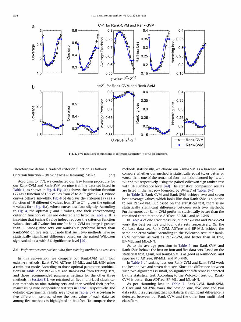
Fig. 3. Five measures as functions of different parameter (g or C) on Emotions.
J. Xu / Pattern Recognition 46 (2013) 885–898894
Therefore we define a tradeoff criterion function as follows:
Criterion function¼ Ranking lossþHamming lossð Þ=2: ð77Þ
According to (77), we conducted our lazy tuning procedure forour Rank-CVM and Rank-SVM on nine training data set listed inTable 1, as shown in Fig. 4. Fig. 4(a) shows the criterion function(77) as a function of 13 g values from 22 to 2�10 given C¼1, whosecurves behave smoothly. Fig. 4(b) displays the criterion (77) as afunction of 10 different C values from 28 to 2�1 given the optimalg values form Fig. 4(a), whose curves oscillate slightly. Accordingto Fig. 4, the optimal g and C values, and their correspondingcriterion function values are detected and listed in Table 2. It isinspiring that tuning C value indeed reduces the criterion functionvalues, since all C values but one for Rank-CVM on Image is greaterthan 1. Among nine sets, our Rank-CVM performs better thanRank-SVM on five sets. But note that such two methods have nostatistically significant difference based on the paired Wilcoxonsign ranked test with 5% significance level [49].
8.4. Performance comparison with four existing methods on test sets
In this sub-section, we compare our Rank-CVM with fourexisting methods: Rank-SVM, ADTree, BP-MLL, and ML-kNN usinga train-test mode. According to those optimal parameter combina-tions in Table 2 for Rank-SVM and Rank-CVM from training sets,and those recommended parameter settings for the other threemethods in Section 8.1, we retrained all five multi-label classifica-tion methods on nine training sets, and then verified their perfor-mance using nine independent test sets in Table 1 respectively. Thedetailed experimental results are shown in Tables 3–7 according tofive different measures, where the best value of each data setamong five methods is highlighted in boldface. To compare these
methods statistically, we choose our Rank-CVM as a baseline, andcompare whether our method is statistically equal to, or better orworse than, one of the remained four methods, denoted by ‘‘¼¼ ’’,‘‘*’’ and ‘‘)’’ respectively, using the paired Wilcoxon sign ranked testwith 5% significance level [49]. The statistical comparison resultsare listed in the last row (denoted by W-test) of Tables 3–7.
In Table 3, Rank-CVM and Rank-SVM achieve two and sevenbest coverage values, which looks like that Rank-SVM is superiorto our Rank-CVM. But based on the statistical test, there is nostatistically significant difference between such two methods.Furthermore, our Rank-CVM performs statistically better than theremained three methods: ADTree, BP-MLL and ML-kNN.
In Table 4 of one error measure, our Rank-CVM and Rank-SVMwork the best on five and four data sets respectively. On theGenbase data set, Rank-CVM, ADTree and BP-MLL achieve thesame one error value. According to the Wilcoxon test, our Rank-CVM performs as well as Rank-SVM, and better than ADTree,BP-MLL and ML-kNN.
As to the average precision in Table 5, our Rank-CVM andRank-SVM behave the best on four and five data sets. Based on thestatistical test, again, our Rank-CVM is as good as Rank-SVM, andsuperior to ADTree, BP-MLL, and ML-kNN.
In Table 6 of ranking loss, our Rank-CVM and Rank-SVM workthe best on two and seven data sets. Since the difference betweensuch two algorithms is small, no significant difference is detectedby the statistical test. According to the Wilcoxon test, our Rank-CVM is better than ADTree, BP-MLL and ML-kNN.
As per Hamming loss in Table 7, Rank-CVM, Rank-SVM,ADTree and ML-kNN work the best on one, five, one and twodata sets. It is surprising that no statistical significant difference isdetected between our Rank-CVM and the other four multi-labelclassifiers.
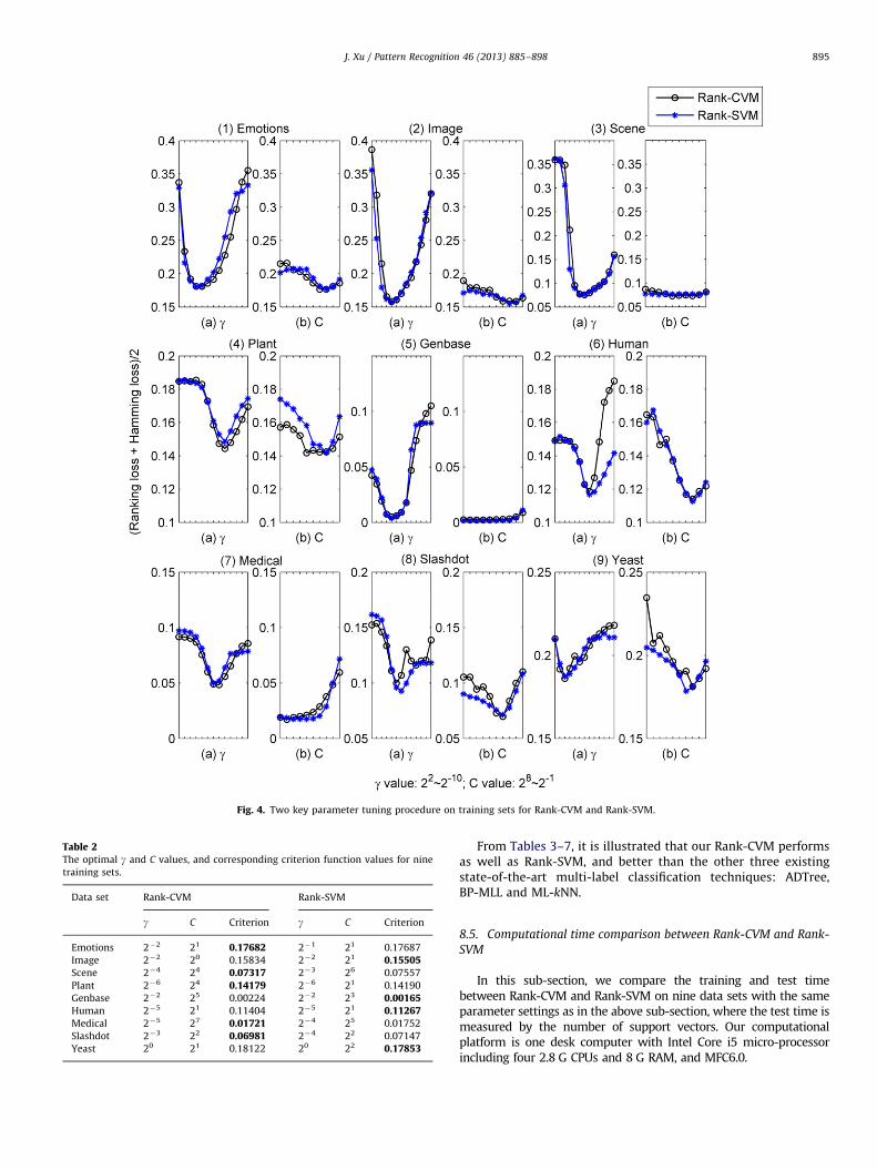
Fig. 4. Two key parameter tuning procedure on training sets for Rank-CVM and Rank-SVM.
Table 2The optimal g and C values, and corresponding criterion function values for nine
training sets.
Data set Rank-CVM Rank-SVM
g C Criterion g C Criterion
Emotions 2�2 21 0.17682 2�1 21 0.17687
Image 2�2 20 0.15834 2�2 21 0.15505Scene 2�4 24 0.07317 2�3 26 0.07557
Plant 2�6 24 0.14179 2�6 21 0.14190
Genbase 2�2 25 0.00224 2�2 23 0.00165Human 2�5 21 0.11404 2�5 21 0.11267Medical 2�5 27 0.01721 2�4 25 0.01752
Slashdot 2�3 22 0.06981 2�4 22 0.07147
Yeast 20 21 0.18122 20 22 0.17853
J. Xu / Pattern Recognition 46 (2013) 885–898 895
From Tables 3–7, it is illustrated that our Rank-CVM performsas well as Rank-SVM, and better than the other three existingstate-of-the-art multi-label classification techniques: ADTree,BP-MLL and ML-kNN.
8.5. Computational time comparison between Rank-CVM and Rank-
SVM
In this sub-section, we compare the training and test timebetween Rank-CVM and Rank-SVM on nine data sets with the sameparameter settings as in the above sub-section, where the test time ismeasured by the number of support vectors. Our computationalplatform is one desk computer with Intel Core i5 micro-processorincluding four 2.8 G CPUs and 8 G RAM, and MFC6.0.
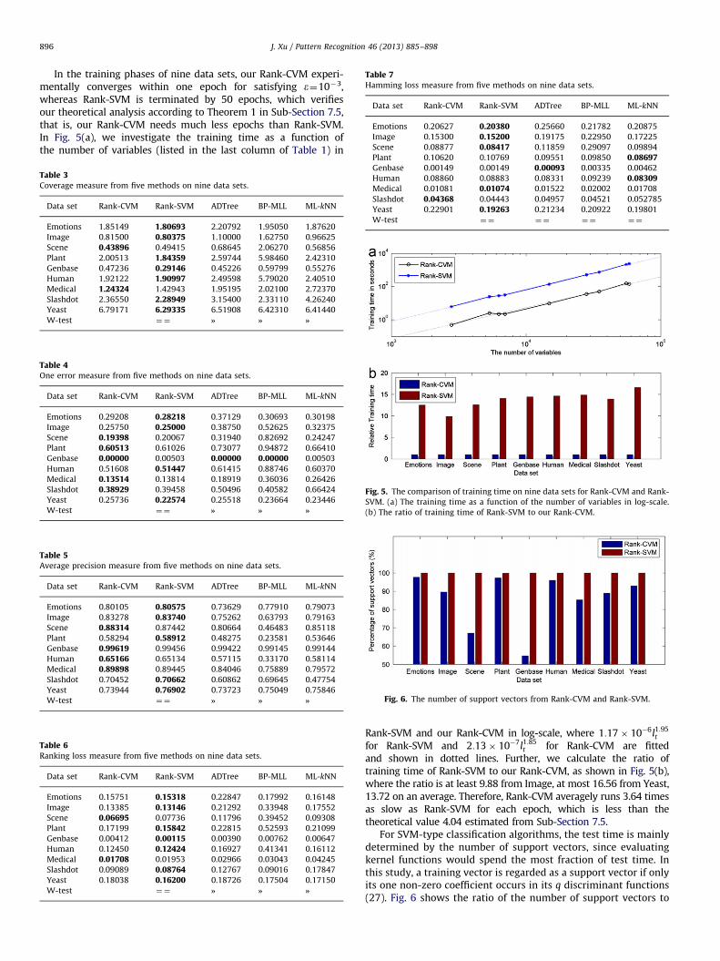
Table 7Hamming loss measure from five methods on nine data sets.
Data set Rank-CVM Rank-SVM ADTree BP-MLL ML-kNN
Emotions 0.20627 0.20380 0.25660 0.21782 0.20875
Image 0.15300 0.15200 0.19175 0.22950 0.17225
Scene 0.08877 0.08417 0.11859 0.29097 0.09894
J. Xu / Pattern Recognition 46 (2013) 885–898896
In the training phases of nine data sets, our Rank-CVM experi-mentally converges within one epoch for satisfying e¼10�3,whereas Rank-SVM is terminated by 50 epochs, which verifiesour theoretical analysis according to Theorem 1 in Sub-Section 7.5,that is, our Rank-CVM needs much less epochs than Rank-SVM.In Fig. 5(a), we investigate the training time as a function ofthe number of variables (listed in the last column of Table 1) in
Table 4One error measure from five methods on nine data sets.
Data set Rank-CVM Rank-SVM ADTree BP-MLL ML-kNN
Emotions 0.29208 0.28218 0.37129 0.30693 0.30198
Image 0.25750 0.25000 0.38750 0.52625 0.32375
Scene 0.19398 0.20067 0.31940 0.82692 0.24247
Plant 0.60513 0.61026 0.73077 0.94872 0.66410
Genbase 0.00000 0.00503 0.00000 0.00000 0.00503
Human 0.51608 0.51447 0.61415 0.88746 0.60370
Medical 0.13514 0.13814 0.18919 0.36036 0.26426
Slashdot 0.38929 0.39458 0.50496 0.40582 0.66424
Yeast 0.25736 0.22574 0.25518 0.23664 0.23446
W-test ¼¼ * * *
Table 5Average precision measure from five methods on nine data sets.
Data set Rank-CVM Rank-SVM ADTree BP-MLL ML-kNN
Emotions 0.80105 0.80575 0.73629 0.77910 0.79073
Image 0.83278 0.83740 0.75262 0.63793 0.79163
Scene 0.88314 0.87442 0.80664 0.46483 0.85118
Plant 0.58294 0.58912 0.48275 0.23581 0.53646
Genbase 0.99619 0.99456 0.99422 0.99145 0.99144
Human 0.65166 0.65134 0.57115 0.33170 0.58114
Medical 0.89898 0.89445 0.84046 0.75889 0.79572
Slashdot 0.70452 0.70662 0.60862 0.69645 0.47754
Yeast 0.73944 0.76902 0.73723 0.75049 0.75846
W-test ¼¼ * * *
Table 6Ranking loss measure from five methods on nine data sets.
Data set Rank-CVM Rank-SVM ADTree BP-MLL ML-kNN
Emotions 0.15751 0.15318 0.22847 0.17992 0.16148
Image 0.13385 0.13146 0.21292 0.33948 0.17552
Scene 0.06695 0.07736 0.11796 0.39452 0.09308
Plant 0.17199 0.15842 0.22815 0.52593 0.21099
Genbase 0.00412 0.00115 0.00390 0.00762 0.00647
Human 0.12450 0.12424 0.16927 0.41341 0.16112
Medical 0.01708 0.01953 0.02966 0.03043 0.04245
Slashdot 0.09089 0.08764 0.12767 0.09016 0.17847
Yeast 0.18038 0.16200 0.18726 0.17504 0.17150
W-test ¼¼ * * *
Plant 0.10620 0.10769 0.09551 0.09850 0.08697Genbase 0.00149 0.00149 0.00093 0.00335 0.00462
Human 0.08860 0.08883 0.08331 0.09239 0.08309Medical 0.01081 0.01074 0.01522 0.02002 0.01708
Slashdot 0.04368 0.04443 0.04957 0.04521 0.052785
Yeast 0.22901 0.19263 0.21234 0.20922 0.19801
W-test ¼¼ ¼¼ ¼¼ ¼¼
Fig. 5. The comparison of training time on nine data sets for Rank-CVM and Rank-
SVM. (a) The training time as a function of the number of variables in log-scale.
(b) The ratio of training time of Rank-SVM to our Rank-CVM.
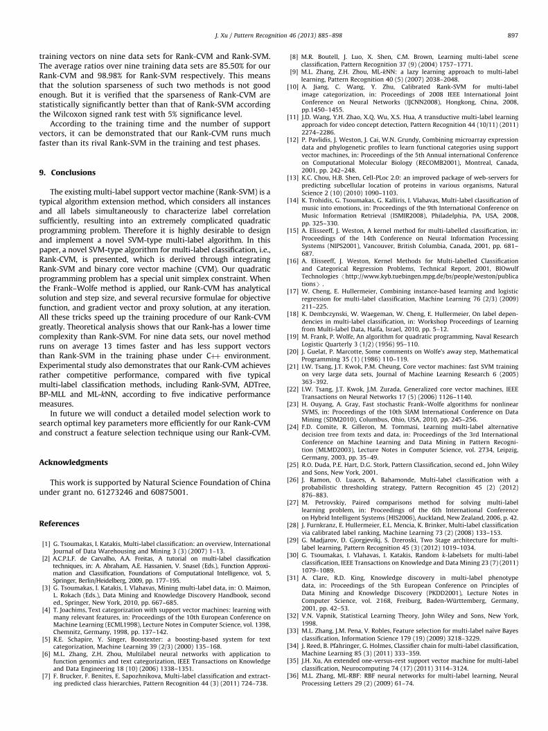
Fig. 6. The number of support vectors from Rank-CVM and Rank-SVM.
Table 3Coverage measure from five methods on nine data sets.
Data set Rank-CVM Rank-SVM ADTree BP-MLL ML-kNN
Emotions 1.85149 1.80693 2.20792 1.95050 1.87620
Image 0.81500 0.80375 1.10000 1.62750 0.96625
Scene 0.43896 0.49415 0.68645 2.06270 0.56856
Plant 2.00513 1.84359 2.59744 5.98460 2.42310
Genbase 0.47236 0.29146 0.45226 0.59799 0.55276
Human 1.92122 1.90997 2.49598 5.79020 2.40510
Medical 1.24324 1.42943 1.95195 2.02100 2.72370
Slashdot 2.36550 2.28949 3.15400 2.33110 4.26240
Yeast 6.79171 6.29335 6.51908 6.42310 6.41440
W-test ¼¼ * * *
Rank-SVM and our Rank-CVM in log-scale, where 1:17� 10�6l1:95t
for Rank-SVM and 2:13� 10�7l1:85t for Rank-CVM are fitted
and shown in dotted lines. Further, we calculate the ratio oftraining time of Rank-SVM to our Rank-CVM, as shown in Fig. 5(b),where the ratio is at least 9.88 from Image, at most 16.56 from Yeast,13.72 on an average. Therefore, Rank-CVM averagely runs 3.64 timesas slow as Rank-SVM for each epoch, which is less than thetheoretical value 4.04 estimated from Sub-Section 7.5.
For SVM-type classification algorithms, the test time is mainlydetermined by the number of support vectors, since evaluatingkernel functions would spend the most fraction of test time. Inthis study, a training vector is regarded as a support vector if onlyits one non-zero coefficient occurs in its q discriminant functions(27). Fig. 6 shows the ratio of the number of support vectors to
J. Xu / Pattern Recognition 46 (2013) 885–898 897
training vectors on nine data sets for Rank-CVM and Rank-SVM.The average ratios over nine training data sets are 85.50% for ourRank-CVM and 98.98% for Rank-SVM respectively. This meansthat the solution sparseness of such two methods is not goodenough. But it is verified that the sparseness of Rank-CVM arestatistically significantly better than that of Rank-SVM accordingthe Wilcoxon signed rank test with 5% significance level.
According to the training time and the number of supportvectors, it can be demonstrated that our Rank-CVM runs muchfaster than its rival Rank-SVM in the training and test phases.
9. Conclusions
The existing multi-label support vector machine (Rank-SVM) is atypical algorithm extension method, which considers all instancesand all labels simultaneously to characterize label correlationsufficiently, resulting into an extremely complicated quadraticprogramming problem. Therefore it is highly desirable to designand implement a novel SVM-type multi-label algorithm. In thispaper, a novel SVM-type algorithm for multi-label classification, i.e.,Rank-CVM, is presented, which is derived through integratingRank-SVM and binary core vector machine (CVM). Our quadraticprogramming problem has a special unit simplex constraint. Whenthe Frank–Wolfe method is applied, our Rank-CVM has analyticalsolution and step size, and several recursive formulae for objectivefunction, and gradient vector and proxy solution, at any iteration.All these tricks speed up the training procedure of our Rank-CVMgreatly. Theoretical analysis shows that our Rank-has a lower timecomplexity than Rank-SVM. For nine data sets, our novel methodruns on average 13 times faster and has less support vectorsthan Rank-SVM in the training phase under Cþþ environment.Experimental study also demonstrates that our Rank-CVM achievesrather competitive performance, compared with five typicalmulti-label classification methods, including Rank-SVM, ADTree,BP-MLL and ML-kNN, according to five indicative performancemeasures.
In future we will conduct a detailed model selection work tosearch optimal key parameters more efficiently for our Rank-CVMand construct a feature selection technique using our Rank-CVM.
Acknowledgments
This work is supported by Natural Science Foundation of Chinaunder grant no. 61273246 and 60875001.
References
[1] G. Tsoumakas, I. Katakis, Multi-label classification: an overview, InternationalJournal of Data Warehousing and Mining 3 (3) (2007) 1–13.
[2] A.C.P.L.F. de Carvalho, A.A. Freitas, A tutorial on multi-label classificationtechniques, in: A. Abraham, A.E. Hassanien, V. Snasel (Eds.), Function Approxi-mation and Classification, Foundations of Computational Intelligence, vol. 5,Springer, Berlin/Heidelberg, 2009, pp. 177–195.
[3] G. Tsoumakas, I. Katakis, I. Vlahavas, Mining multi-label data, in: O. Maimon,L. Rokach (Eds.), Data Mining and Knowledge Discovery Handbook, seconded., Springer, New York, 2010, pp. 667–685.
[4] T. Joachims, Text categorization with support vector machines: learning withmany relevant features, in: Proceedings of the 10th European Conference onMachine Learning (ECML1998), Lecture Notes in Computer Science, vol. 1398,Chemnitz, Germany, 1998, pp. 137–142.
[5] R.E. Schapire, Y. Singer, Boostexter: a boosting-based system for textcategorization, Machine Learning 39 (2/3) (2000) 135–168.
[6] M.L. Zhang, Z.H. Zhou, Multilabel neural networks with application tofunction genomics and text categorization, IEEE Transactions on Knowledgeand Data Engineering 18 (10) (2006) 1338–1351.
[7] F. Brucker, F. Benites, E. Sapozhnikova, Multi-label classification and extract-ing predicted class hierarchies, Pattern Recognition 44 (3) (2011) 724–738.
[8] M.R. Boutell, J. Luo, X. Shen, C.M. Brown, Learning multi-label sceneclassification, Pattern Recognition 37 (9) (2004) 1757–1771.
[9] M.L. Zhang, Z.H. Zhou, ML-kNN: a lazy learning approach to multi-labellearning, Pattern Recognition 40 (5) (2007) 2038–2048.
[10] A. Jiang, C. Wang, Y. Zhu, Calibrated Rank-SVM for multi-labelimage categorization, in: Proceedings of 2008 IEEE International JointConference on Neural Networks (IJCNN2008), Hongkong, China, 2008,pp.1450–1455.
[11] J.D. Wang, Y.H. Zhao, X.Q. Wu, X.S. Hua, A transductive multi-label learningapproach for video concept detection, Pattern Recognition 44 (10/11) (2011)2274–2286.
[12] P. Pavlidis, J. Weston, J. Cai, W.N. Grundy, Combining microarray expressiondata and phylogenetic profiles to learn functional categories using supportvector machines, in: Proceedings of the 5th Annual international Conferenceon Computational Molecular Biology (RECOMB2001), Montreal, Canada,2001, pp. 242–248.
[13] K.C. Chou, H.B. Shen, Cell-PLoc 2.0: an improved package of web-servers forpredicting subcellular location of proteins in various organisms, NaturalScience 2 (10) (2010) 1090–1103.
[14] K. Trohidis, G. Tsoumakas, G. Kalliris, I. Vlahavas, Multi-label classification ofmusic into emotions, in: Proceedings of the 9th International Conference onMusic Information Retrieval (ISMIR2008), Philadelphia, PA, USA, 2008,pp. 325–330.
[15] A. Elisseeff, J. Weston, A kernel method for multi-labelled classification, in:Proceedings of the 14th Conference on Neural Information ProcessingSystems (NIPS2001), Vancouver, British Columbia, Canada, 2001, pp. 681–687.
[16] A. Elisseeff, J. Weston, Kernel Methods for Multi-labelled Classificationand Categorical Regression Problems, Technical Report, 2001, BIOwulfTechnologies /http://www.kyb.tuebingen.mpg.de/bs/people/weston/publicationsS .
[17] W. Cheng, E. Hullermeier, Combining instance-based learning and logisticregression for multi-label classification, Machine Learning 76 (2/3) (2009)211–225.
[18] K. Dembczynski, W. Waegeman, W. Cheng, E. Hullermeier, On label depen-dencies in multi-label classification, in: Workshop Proceedings of Learningfrom Multi-label Data, Haifa, Israel, 2010, pp. 5–12.
[19] M. Frank, P. Wolfe, An algorithm for quadratic programming, Naval ResearchLogistic Quarterly 3 (1/2) (1956) 95–110.
[20] J. Guelat, P. Marcotte, Some comments on Wolfe’s away step, MathematicalProgramming 35 (1) (1986) 110–119.
[21] I.W. Tsang, J.T. Kwok, P.M. Cheung, Core vector machines: fast SVM trainingon very large data sets, Journal of Machine Learning Research 6 (2005)363–392.
[22] I.W. Tsang, J.T. Kwok, J.M. Zurada, Generalized core vector machines, IEEETransactions on Neural Networks 17 (5) (2006) 1126–1140.
[23] H. Ouyang, A. Gray, Fast stochastic Frank–Wolfe algorithms for nonlinearSVMS, in: Proceedings of the 10th SIAM International Conference on DataMining (SDM2010), Columbus, Ohio, USA, 2010, pp. 245–256.
[24] F.D. Comite, R. Gilleron, M. Tommasi, Learning multi-label alternativedecision tree from texts and data, in: Proceedings of the 3rd InternationalConference on Machine Learning and Data Mining in Pattern Recogni-tion (MLMD2003), Lecture Notes in Computer Science, vol. 2734, Leipzig,Germany, 2003, pp. 35–49.
[25] R.O. Duda, P.E. Hart, D.G. Stork, Pattern Classification, second ed., John Wileyand Sons, New York, 2001.
[26] J. Ramon, O. Luaces, A. Bahamonde, Multi-label classification with aprobabilistic thresholding strategy, Pattern Recognition 45 (2) (2012)876–883.
[27] M. Petrovskiy, Paired comparisons method for solving multi-labellearning problem, in: Proceedings of the 6th International Conferenceon Hybrid Intelligent Systems (HIS2006), Auckland, New Zealand, 2006, p. 42.
[28] J. Furnkranz, E. Hullermeier, E.L. Mencia, K. Brinker, Multi-label classificationvia calibrated label ranking, Machine Learning 73 (2) (2008) 133–153.
[29] G. Madjarov, D. Gjorgjevikj, S. Dzeroski, Two Stage architecture for multi-label learning, Pattern Recognition 45 (3) (2012) 1019–1034.
[30] G. Tsoumakas, I. Vlahavas, I. Katakis, Random k-labelsets for multi-labelclassification, IEEE Transactions on Knowledge and Data Mining 23 (7) (2011)1079–1089.
[31] A. Clare, R.D. King, Knowledge discovery in multi-label phenotypedata, in: Proceedings of the 5th European Conference on Principles ofData Mining and Knowledge Discovery (PKDD2001), Lecture Notes inComputer Science, vol. 2168, Freiburg, Baden-Wurttemberg, Germany,2001, pp. 42–53.
[32] V.N. Vapnik, Statistical Learning Theory, John Wiley and Sons, New York,1998.
[33] M.L. Zhang, J.M. Pena, V. Robles, Feature selection for multi-label naıve Bayesclassification, Information Science 179 (19) (2009) 3218–3229.
[34] J. Reed, B. Pfahringer, G. Holmes, Classifier chain for multi-label classification,Machine Learning 85 (3) (2011) 333–359.
[35] J.H. Xu, An extended one-versus-rest support vector machine for multi-labelclassification, Neurocomputing 74 (17) (2011) 3114–3124.
[36] M.L. Zhang, ML-RBF: RBF neural networks for multi-label learning, NeuralProcessing Letters 29 (2) (2009) 61–74.
J. Xu / Pattern Recognition 46 (2013) 885–898898
[37] L. Wang, M. Chang, J. Feng, Parallel and sequential support vector machinesfor multi-label classification, International Journal of Information Technology11 (9) (2005) 11–18.
[38] S.P. Wan, J.H. Xu, A multi-label classification algorithm based on triple classsupport vector machine, in: Proceedings of 2007 IEEE International Con-ference on Wavelet Analysis and Pattern Recognition (ICPRWA2007), Beijing,China, 2007, pp. 1447–1452.
[39] J.Y. Li, J.H. Xu, A fast multi-label classification algorithm based on doublelabel support vector machine, in: Proceedings of 2009 International Con-ference on Computational Intelligence and Security (CIS2009), vol. 2, Beijing,China, 2009, pp. 30–35.
[40] C.C. Chang, C.J. Lin, Training nu-support vector classifiers: theory andalgorithm, Neural Computation 13 (9) (2001) 2119–2147.
[41] R.E. Fan, P.H. Chen, C.J. Lin, Working set selection using second orderinformation for training support vector machines, Journal of Machine Learn-ing Research 6 (2005) 1889–1918.
[42] F.D. Comite, R. Gilleron, M. Tommasi, ADTree, 2003 /http://www.grappa.
univlille3.fr/ftp/Softs/ADTree.tgzS.[43] M.L. Zhang, Matlab software of BP-MLL and ML-kNN, and Image data set,
2009 /http://cse.seu.edu.cn/people/zhangmlS.[44] S. Stiena, LPSOL5.5, 2006 /http://www.cs.sunysb.edu/algorithm/implement/
lpsolve/implement.shtmlS.[45] G. Tsoumakas, Multi-label data sets, 2009 /http://mulan.sourceforge.net/
datasets.htmlS.[46] J. Read, Slashdot data set, 2011 /http://meka.sourceforge.net/#datasetsS.[47] H.B. Shen, Cell_PLoc 2.0 data sets, 2010 /http://www.csbio.sjtu.edu.cn/
bioinf/Cell-PLoc-2/DataS.[48] P.F. Du , PseAAC-Builder, 2011 /http://www.sourceforge.net/projects/pseb/
filesS.[49] J. Demsar, Statistical comparison of classifiers over multiple data sets, Journal
of Machine Learning Research 7 (2006) 1–30.
Jianhua Xu received his Ph.D. in Pattern Recognition and Intelligent Systems in 2002 (Department of Automation, Tsinghua University, Beijing, China). Since 2005, he is aprofessor in Computer Science, Nanjing Normal University, Nanjing, China. From September 2008 to September 2009, he was a visiting scholar at Department of Statistics,Harvard University, Cambridge MA, USA. His research interests are focused on pattern recognition, machine learning, and their applications to bioinformatics.