FAST MAPPING WITH µ-XRF

In the February 2013 issue of the Elements Toolkit, I reported on field-portable XRF devices, which have become available over the past decade or so. This issue’s Toolkit is devoted to a related technology, which, though labora-tory based, has likewise seen impressive leaps over recent years: mapping micron-scale X-ray fl uorescence (µ-XRF). Both methods work on the same principle, whereby primary X-rays interact with the sample material, generating characteristic secondary X-rays that are used to quantify the elemental composition of the material under investigation. In the case of mapping µ-XRF instruments, a fi nely focused primary X-ray source is employed, resulting in spatially resolved chemical information at a length scale reaching down to a few tens of micrometers. Though not competing with the scanning electron microscope (SEM) in terms of spatial resolution, µ-XRF has a number of properties that may make it decisively attrac-tive for certain applications.

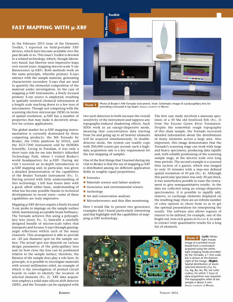
The global market for µ-XRF mapping instru-mentation is currently dominated by three competing products: the M4 Tornado by Bruker, the Orbis platform by EDAX, and the XGT-7200 instrument sold by HORIBA Scientifi c. Living in Potsdam, it was only a short train ride for me into Berlin’s Adlershof Technology Park, where I visited Bruker’s world headquarters for µ-XRF. During my visit I received an in-depth introduction to µ-XRF mapping and, in particular, was given a detailed demonstration of the capabilities of the Bruker Tornado instrument (FIG. 1). Having arrived with little understanding of this technology, I left four hours later with a good, albeit rather basic, understanding of what has become possible thanks to technical developments in recent years—some of these capabilities are truly impressive.

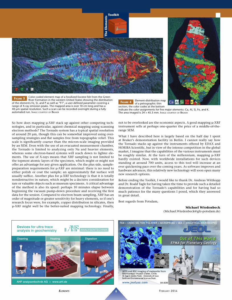
Mapping µ-XRF devices require a fi nely focused X-ray probe to impinge on the sample surface while maintaining acceptable beam brilliance. The Tornado achieves this using a polycapil-lary lens (inset, FIG. 1), basically a carefully designed bundle of micron-scale tubes that transports and focuses X-rays through grazing-angle refl ections within each of the many channels. This arrangement is able to provide an ~20 µm diameter spot on the sample sur-face. The actual spot size depends on various design parameters of the polycapillary lens and on how close the lens can be positioned relative to the sample surface; therefore, the fl atness of the sample does play a role here. In principle, it is possible to investigate materials with several millimeters relief, an example of which is the investigation of printed circuit boards in order to identify the location of selected elements (FIG. 2). XRF data acquisi-tion employs a solid-state silicon drift detector (SDD), and the Tornado can be equipped with

two such detectors to both increase the overall sensitivity of the instrument and suppress any topography-induced shadowing effects. Such SDDs work in an energy-dispersive mode, meaning that concentration data starting from Na and going up to all heavier elements will be acquired simultaneously. In double-detector mode, the system can readily cope with 200,000 counts per second; such a high-data acquisition rate is a key requirement for the fast mapping of samples.

One of the fi rst things that I learned during my visit to Bruker is that the use of mapping µ-XRF is distributed among six different application fi elds in roughly equal proportions:

Forensics

Materials science and failure analysis

Geoscience and environmental science

Archeology

Art and conservation analyses

Microelectronics and thin fi lm monitoring

Here I would like to present two geoscience examples that I found particularly interesting and that highlight well the capabilities of map-ping µ-XRF technology.

The fi rst case study involved a museum spec-imen of a 50 Ma old fossilized fi sh (FIG. 3) from the Eocene Green River Formation. Despite the somewhat rough topography of this shale sample, the Tornado recovered detailed information about the distributions of many elements across a large area. Also important, this image demonstrates that the Tornado’s scanning stage can work with large and heavy specimens, producing data rapidly and, with reliable positioning of the scanning sample stage, at the micron scale over long time periods. The second example is a scanned thin section of a gneiss, which was imaged in only 35 minutes with a step-size defi ned spatial resolution of 50 µm (FIG. 4). Although this particular specimen was only 30 µm thick, it was nonetheless possible to tune the instru-ment to give semiquantitative results. As the data are collected using an energy-dispersive spectrometer, it is possible to rapidly add, remove, or exchange elements displayed on the resulting map; there are an infi nite number of color options to chose from so as to get the optimal presentation for interpreting the results. The software also allows regions of interest to be defi ned, for example, one of the bright red, iron-rich grains in FIGURE 4, in order to extract truly quantitative results for a long list of elements.

FIGURE 1 Photo of Bruker’s M4 Tornado instrument. Inset: Schematic image of a polycapillary lens for providing a focused X-ray beam. IMAGES COURTESY OF BRUKER

FIGURE 2 (Left) White-light mosaic

image of a printed circuit board from a wristwatch acquired using the white-light imaging mode provided by the Tornado; a 1 mm scale bar is shown at the bottom right of the image. (Right) Spatial distribution of seven selected elements (Ca, Fe, Cu, Ag, Ba, Au, Pb; see color codes), for which 1 hour of data acquisition was required. The topographic relief of the sample is about 2 mm. IMAGES COURTESY OF BRUKER

ELEMENTS FEBRUARY 20145

So how does mapping µ-XRF stack up against other competing tech-nologies, and in particular, against chemical mapping using scanning electron methods? The Tornado system has a typical spatial resolution of around 20 µm, though this can be somewhat improved using over-sampling strategies and fl at samples free from topographic relief. This scale is signifi cantly coarser than the micron-scale imaging provided by an SEM. Even with the use of an evacuated measurement chamber, the Tornado is limited to analyzing only Na and heavier elements, whereas some electron-based systems will reach down to lighter ele-ments. The use of X-rays means that XRF sampling is not limited to the topmost atomic layers of the specimen, which might or might not offer an advantage for any given application. On the plus side, sample-preparation requirements for µ-XRF are minimal: there is no need to either polish or coat the sample; an approximately fl at surface will usually suffi ce. Another plus for µ-XRF technology is that it is totally nondestructive in nature, which might be a decisive consideration for rare or valuable objects such as museum specimens. A critical advantage of the method is also its speed: perhaps 10 minutes elapse between beginning the vacuum pump-down procedure and receiving the fi rst data for the session. Compared to electron beam sampling, XRF has an order of magnitude or greater sensitivity for heavy elements, so if one’s research focus were, for example, copper distribution in silicates, then µ-XRF might well be the better-suited mapping technology. Finally,

not to be overlooked are the economic aspects. A good mapping µ-XRF instrument sells at perhaps one-quarter the price of a middle-of-the-range SEM.

What I have described here is largely based on the half day I spent at Bruker’s demonstration facility in Berlin. I cannot really say how the Tornado stacks up against the instruments offered by EDAX and HORIBA Scientifi c, but in view of the intense competition in the global market, I imagine that the capabilities of the various instruments must be roughly similar. At the turn of the millennium, mapping µ-XRF hardly existed. Now, with worldwide installations for such devices standing at around 700 units, access to this tool will increase at an ever quickening pace over the coming years. As software improves and hardware advances, this relatively new technology will soon open many new research options.

Before ending the Toolkit, I would like to thank Dr. Andreas Wittkopp and Dr. Roald Tagle for having taken the time to provide such a detailed demonstration of the Tornado’s capabilities and for having had so much patience for the many questions I posed, which they answered in great detail.

Best regards from Potsdam,

Michael Wiedenbeck (Michael.Wiedenbeck@gfz-potsdam.de)

FIGURE 4 Element-distribution map of a petrographic thin

section; the color codes at the bottom indicate the color assignments for fi ve major elements: Ca, Al, Si, Fe, and K. The area imaged is 24 × 45.3 mm. IMAGE COURTESY OF BRUKER

FIGURE 3 Color-coded element map of a fossilized Eocene fi sh from the Green River Formation in the western United States showing the distribution

of the elements Fe, Sr, and P as well as “F1”, a user-defi ned parameter covering a range of X-ray emission peaks. The mapped area is over 10 cm long and has a 40 µm spatial resolution. Such a scan can be recorded overnight during a fully automated run. IMAGE COURTESY OF BRUKER

Devices for ultra trace analysis in geochemistry

AHF analysentechnik AG :: www.ahf.de

Cleaning DigestionHeating

METAL-FREE

ELEMENTS FEBRUARY 20146