Embed Size (px)
Citation preview
Fast lp–regression in a Data Stream
Christian Sohler (TU Dortmund)
David Woodruff (IBM Almaden)
2
Overview
Massive data sets Streaming algorithms Regression Clarkson‘s algorithm Our results Subspace embeddings Noisy sampling
3
Massive data sets
Examples Internet traffic logs Financial data etc.
4
Streaming algorithms
Scenario Data arrives sequentially at a high rate and in arbitrary order Data is too large to be stored completely or is stored in secondary memory
(where streaming is the fastest way of accessing the data) We want some information about the data
Algorithmic requirements Data must be processed quickly Only a summary of the data can be stored Goal: Approximate some statistics of the data
5
Streaming algorithms
The turnstile model Input: A sequence of updates to an object (vector, matrix, database, etc.) Output: An approximation of some statistics of the object Space: significantly sublinear in input size Overall time: near-linear in input size
6
Streaming algorithms
Example Approximating the number of users of a search engine Each user has its ID (IP-address) Take the vector v of all valid IP-addresses as the object Entries of v: #queries submitted to search engine Whenever a user submits a query, increment v at the entry corresponding to
the submitting IP-address Required statistic: # non-zero entries in the current vector
7
Regression analysis
Regression Statistical method to study dependencies between variables in the
presence of noise.
8
Regression analysis
Linear Regression Statistical method to study linear dependencies between variables in the
presence of noise.
9
Regression analysis
Linear Regression Statistical method to study linear dependencies between variables in the
presence of noise.
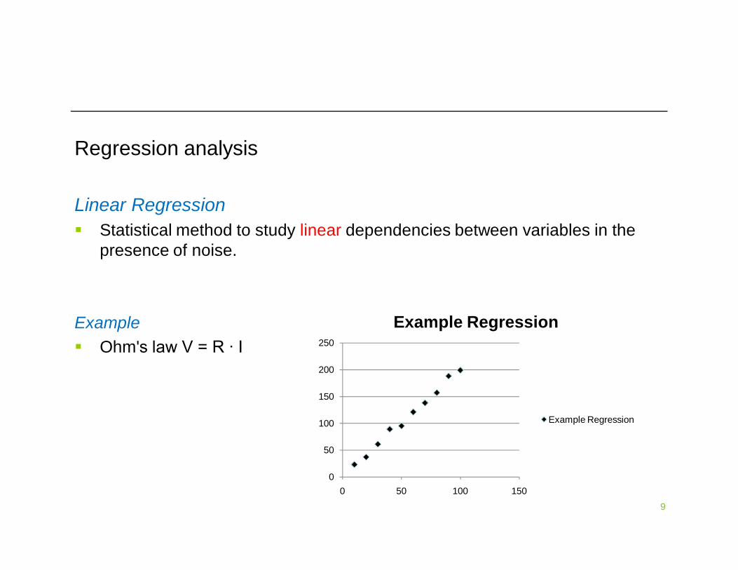
Example Ohm's law V = R ∙ I
0
50
100
150
200
250
0 50 100 150
Example Regression
Example Regression
10
Regression analysis
Linear Regression Statistical method to study linear dependencies between variables in the
presence of noise.
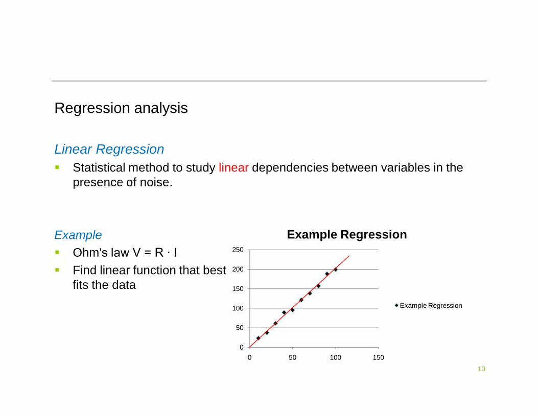
Example Ohm's law V = R ∙ I Find linear function that best
fits the data
0
50
100
150
200
250
0 50 100 150
Example Regression
Example Regression
11
Regression analysis
Linear Regression Statistical method to study linear dependencies between variables in the
presence of noise.
Standard Setting One measured variable y A set of predictor variables x ,…, x Assumption:
y = b + b x + … + b x + e e is assumed to be a noise (random) variable and the b are model
parameters
1 d
1 1 d d0
j
12
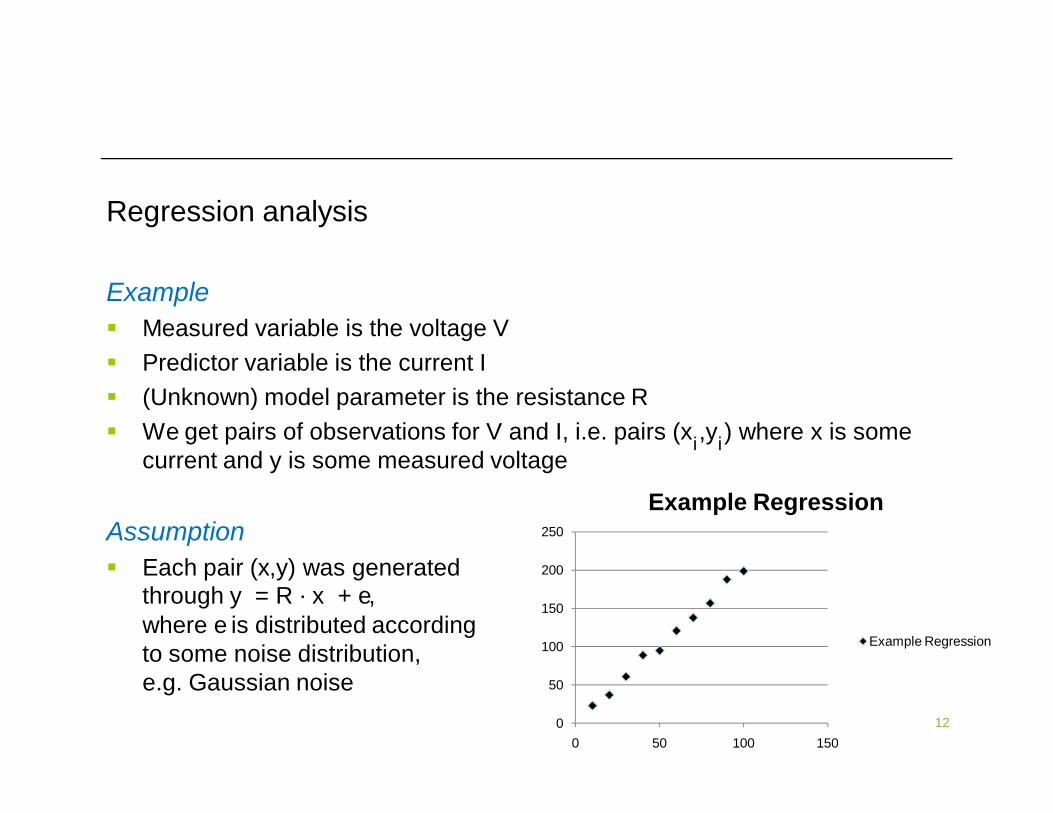
Regression analysis
Example Measured variable is the voltage V Predictor variable is the current I (Unknown) model parameter is the resistance R We get pairs of observations for V and I, i.e. pairs (x ,y ) where x is some
current and y is some measured voltage
Assumption Each pair (x,y) was generated
through y = R ∙ x + e,where e is distributed according to some noise distribution, e.g. Gaussian noise
i i
0
50
100
150
200
250
0 50 100 150
Example Regression
Example Regression
13
Regression analysis
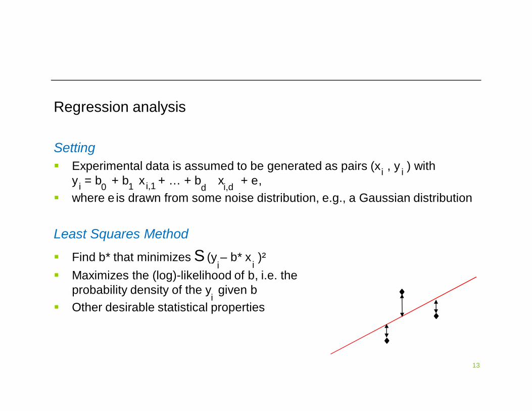
Setting Experimental data is assumed to be generated as pairs (x , y ) with
y = b + b x + … + b x + e, where e is drawn from some noise distribution, e.g., a Gaussian distribution
Least Squares Method
Find b* that minimizes S (y – b* x )² Maximizes the (log)-likelihood of b, i.e. the
probability density of the y given b Other desirable statistical properties
i ii 0 1 i,1 d i,d
i i
i
14
Regression analysis
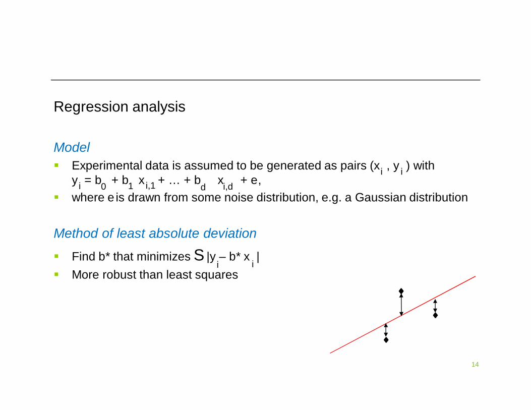
Model Experimental data is assumed to be generated as pairs (x , y ) with
y = b + b x + … + b x + e, where e is drawn from some noise distribution, e.g. a Gaussian distribution
Method of least absolute deviation
Find b* that minimizes S |y – b* x | More robust than least squares
i ii 0 1 i,1 d i,d
i i
15
Regression analysis
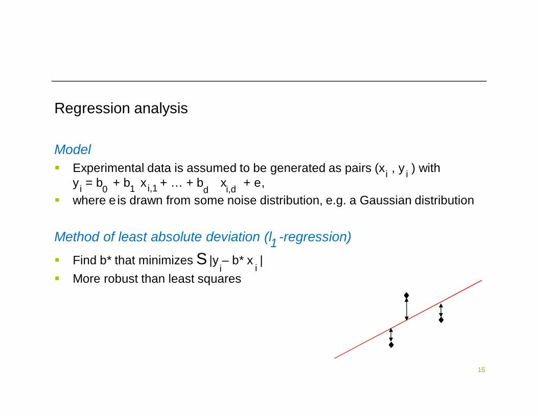
Model Experimental data is assumed to be generated as pairs (x , y ) with
y = b + b x + … + b x + e, where e is drawn from some noise distribution, e.g. a Gaussian distribution
Method of least absolute deviation (l -regression)
Find b* that minimizes S |y – b* x | More robust than least squares
i ii 0 1 i,1 d i,d
i i
1
16
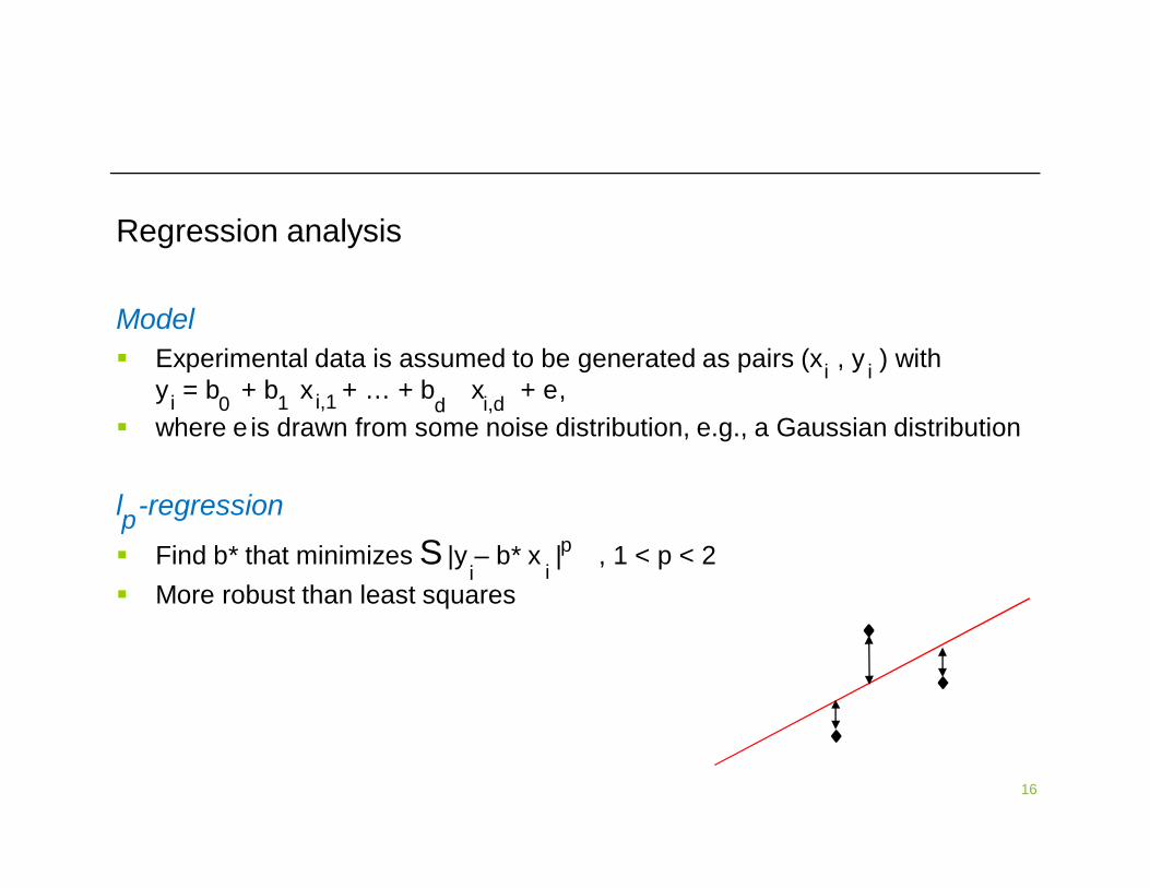
Regression analysis
Model Experimental data is assumed to be generated as pairs (x , y ) with
y = b + b x + … + b x + e, where e is drawn from some noise distribution, e.g., a Gaussian distribution
l -regression
Find b* that minimizes S |y – b* x | , 1 < p < 2 More robust than least squares
i ii 0 1 i,1 d i,d
i ip
p
17
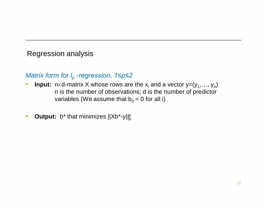
Regression analysis
Matrix form for lp -regression, 1≤p≤2 Input: nd-matrix X whose rows are the xi and a vector y=(y1,…, yn)
n is the number of observations; d is the number of predictor variables (We assume that b0 = 0 for all i)
Output: b* that minimizes ||Xb*-y||pp
18
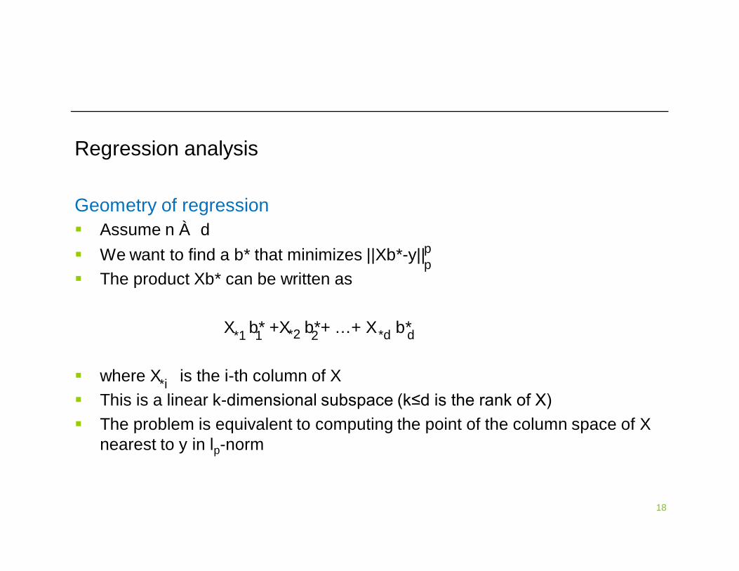
Regression analysis
Geometry of regression Assume n À d We want to find a b* that minimizes ||Xb*-y|| The product Xb* can be written as
X b* +X b*+ …+ X b*
where X is the i-th column of X This is a linear k-dimensional subspace (k≤d is the rank of X) The problem is equivalent to computing the point of the column space of X
nearest to y in lp-norm
*1 *2 *d1 2 d
*i
pp
19
Regression analysis
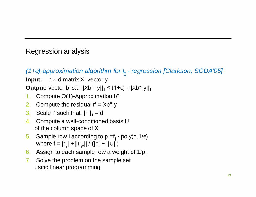
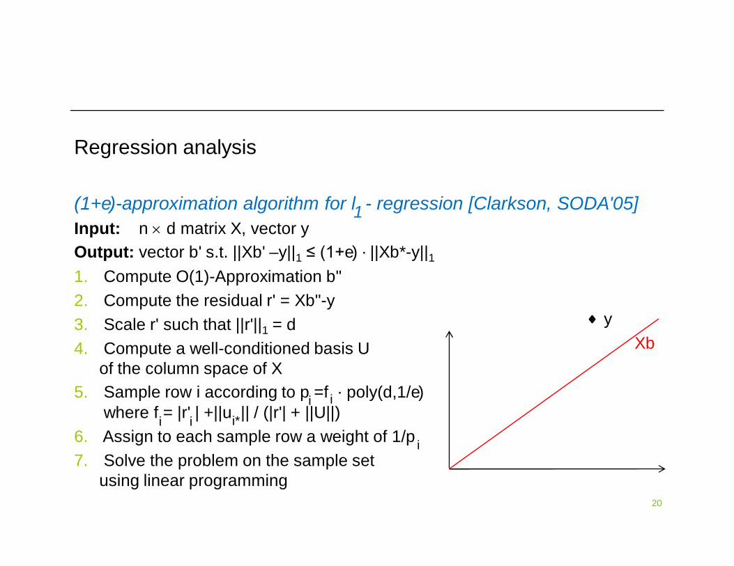
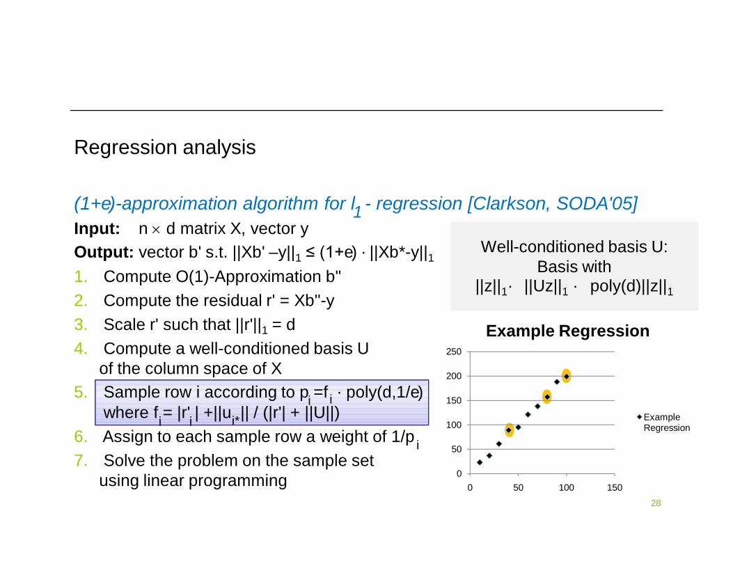
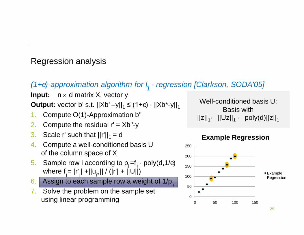
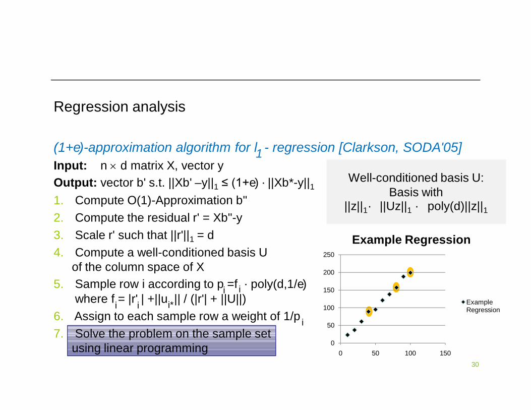
(1+e)-approximation algorithm for l - regression [Clarkson, SODA'05]Input: n d matrix X, vector yOutput: vector b' s.t. ||Xb' –y||1 ≤ (1+e) ∙ ||Xb*-y||11. Compute O(1)-Approximation b"2. Compute the residual r' = Xb"-y 3. Scale r' such that ||r'||1 = d4. Compute a well-conditioned basis U
of the column space of X5. Sample row i according to p =f ∙ poly(d,1/e)
where f = |r' | +||u || / (|r'| + ||U||)6. Assign to each sample row a weight of 1/p7. Solve the problem on the sample set
using linear programming
1
i i
i i i*
i
20
Regression analysis
1
yXb
i i
i i i*
i
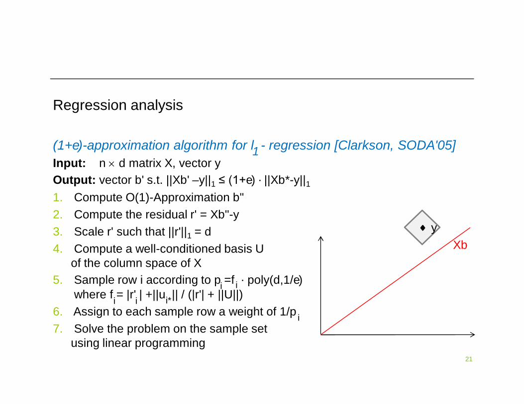
(1+e)-approximation algorithm for l - regression [Clarkson, SODA'05]Input: n d matrix X, vector yOutput: vector b' s.t. ||Xb' –y||1 ≤ (1+e) ∙ ||Xb*-y||11. Compute O(1)-Approximation b"2. Compute the residual r' = Xb"-y 3. Scale r' such that ||r'||1 = d4. Compute a well-conditioned basis U
of the column space of X5. Sample row i according to p =f ∙ poly(d,1/e)
where f = |r' | +||u || / (|r'| + ||U||)6. Assign to each sample row a weight of 1/p7. Solve the problem on the sample set
using linear programming
21
Regression analysis
1
yXb
i i
i i i*
i
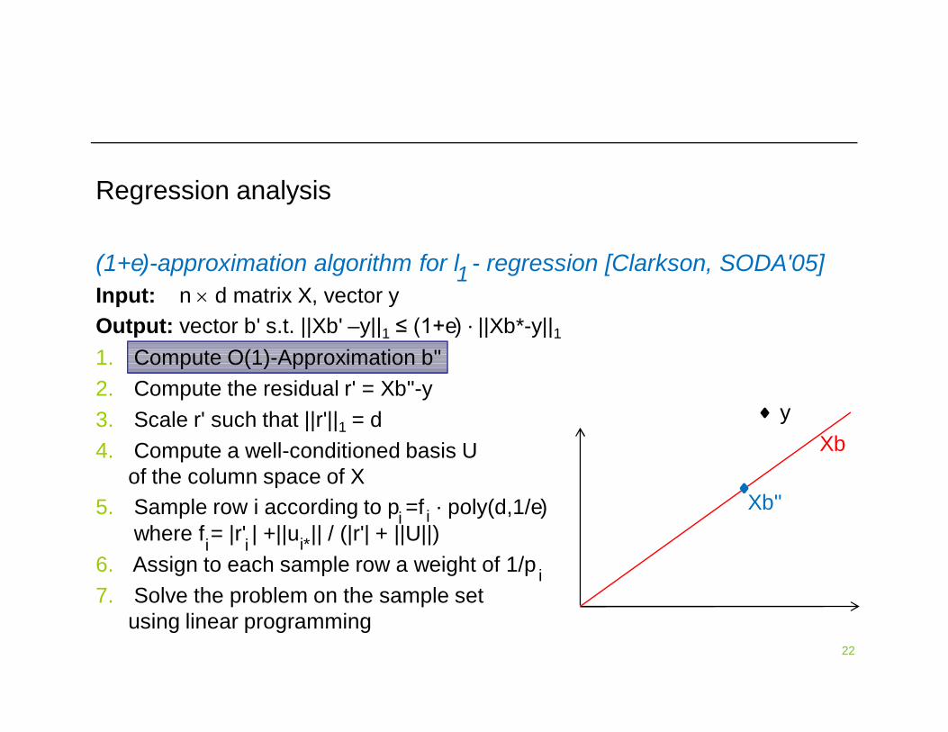
(1+e)-approximation algorithm for l - regression [Clarkson, SODA'05]Input: n d matrix X, vector yOutput: vector b' s.t. ||Xb' –y||1 ≤ (1+e) ∙ ||Xb*-y||11. Compute O(1)-Approximation b"2. Compute the residual r' = Xb"-y 3. Scale r' such that ||r'||1 = d4. Compute a well-conditioned basis U
of the column space of X5. Sample row i according to p =f ∙ poly(d,1/e)
where f = |r' | +||u || / (|r'| + ||U||)6. Assign to each sample row a weight of 1/p7. Solve the problem on the sample set
using linear programming
22
Regression analysis
1
Xby
Xb"i i
i i i*
i
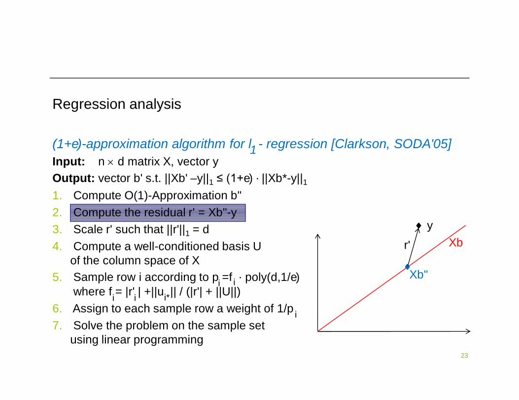
(1+e)-approximation algorithm for l - regression [Clarkson, SODA'05]Input: n d matrix X, vector yOutput: vector b' s.t. ||Xb' –y||1 ≤ (1+e) ∙ ||Xb*-y||11. Compute O(1)-Approximation b"2. Compute the residual r' = Xb"-y 3. Scale r' such that ||r'||1 = d4. Compute a well-conditioned basis U
of the column space of X5. Sample row i according to p =f ∙ poly(d,1/e)
where f = |r' | +||u || / (|r'| + ||U||)6. Assign to each sample row a weight of 1/p7. Solve the problem on the sample set
using linear programming
23
Regression analysis
1
Xby
Xb"
r'
i
ii
i i*
i
(1+e)-approximation algorithm for l - regression [Clarkson, SODA'05]Input: n d matrix X, vector yOutput: vector b' s.t. ||Xb' –y||1 ≤ (1+e) ∙ ||Xb*-y||11. Compute O(1)-Approximation b"2. Compute the residual r' = Xb"-y 3. Scale r' such that ||r'||1 = d4. Compute a well-conditioned basis U
of the column space of X5. Sample row i according to p =f ∙ poly(d,1/e)
where f = |r' | +||u || / (|r'| + ||U||)6. Assign to each sample row a weight of 1/p7. Solve the problem on the sample set
using linear programming
24
Regression analysis
1
Xb
r'i
ii
i*
i
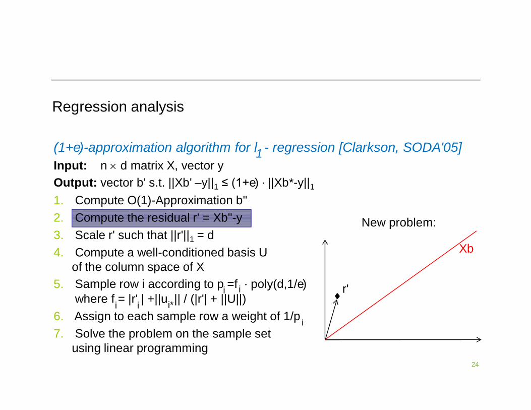
New problem:
i
(1+e)-approximation algorithm for l - regression [Clarkson, SODA'05]Input: n d matrix X, vector yOutput: vector b' s.t. ||Xb' –y||1 ≤ (1+e) ∙ ||Xb*-y||11. Compute O(1)-Approximation b"2. Compute the residual r' = Xb"-y 3. Scale r' such that ||r'||1 = d4. Compute a well-conditioned basis U
of the column space of X5. Sample row i according to p =f ∙ poly(d,1/e)
where f = |r' | +||u || / (|r'| + ||U||)6. Assign to each sample row a weight of 1/p7. Solve the problem on the sample set
using linear programming
25
Regression analysis
1
Xb
r'i
ii
i*
i
i
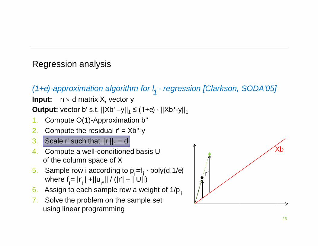
(1+e)-approximation algorithm for l - regression [Clarkson, SODA'05]Input: n d matrix X, vector yOutput: vector b' s.t. ||Xb' –y||1 ≤ (1+e) ∙ ||Xb*-y||11. Compute O(1)-Approximation b"2. Compute the residual r' = Xb"-y 3. Scale r' such that ||r'||1 = d4. Compute a well-conditioned basis U
of the column space of X5. Sample row i according to p =f ∙ poly(d,1/e)
where f = |r' | +||u || / (|r'| + ||U||)6. Assign to each sample row a weight of 1/p7. Solve the problem on the sample set
using linear programming
26
Regression analysis
1
Xb
r'i
ii
i*
i
i
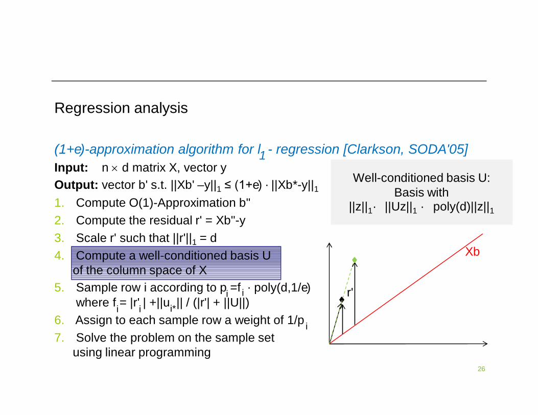
(1+e)-approximation algorithm for l - regression [Clarkson, SODA'05]Input: n d matrix X, vector yOutput: vector b' s.t. ||Xb' –y||1 ≤ (1+e) ∙ ||Xb*-y||11. Compute O(1)-Approximation b"2. Compute the residual r' = Xb"-y 3. Scale r' such that ||r'||1 = d4. Compute a well-conditioned basis U
of the column space of X5. Sample row i according to p =f ∙ poly(d,1/e)
where f = |r' | +||u || / (|r'| + ||U||)6. Assign to each sample row a weight of 1/p7. Solve the problem on the sample set
using linear programming
Well-conditioned basis U:Basis with
||z||1· ||Uz||1 · poly(d)||z||1
27
0
50
100
150
200
250
0 50 100 150
Example Regression
Example Regression
Regression analysis
1
i
ii
i*
i
i
(1+e)-approximation algorithm for l - regression [Clarkson, SODA'05]Input: n d matrix X, vector yOutput: vector b' s.t. ||Xb' –y||1 ≤ (1+e) ∙ ||Xb*-y||11. Compute O(1)-Approximation b"2. Compute the residual r' = Xb"-y 3. Scale r' such that ||r'||1 = d4. Compute a well-conditioned basis U
of the column space of X5. Sample row i according to p =f ∙ poly(d,1/e)
where f = |r' | +||u || / (|r'| + ||U||)6. Assign to each sample row a weight of 1/p7. Solve the problem on the sample set
using linear programming
Well-conditioned basis U:Basis with
||z||1· ||Uz||1 · poly(d)||z||1
28
Regression analysis
1
i
ii
i*
i
i
0
50
100
150
200
250
0 50 100 150
Example Regression
Example Regression
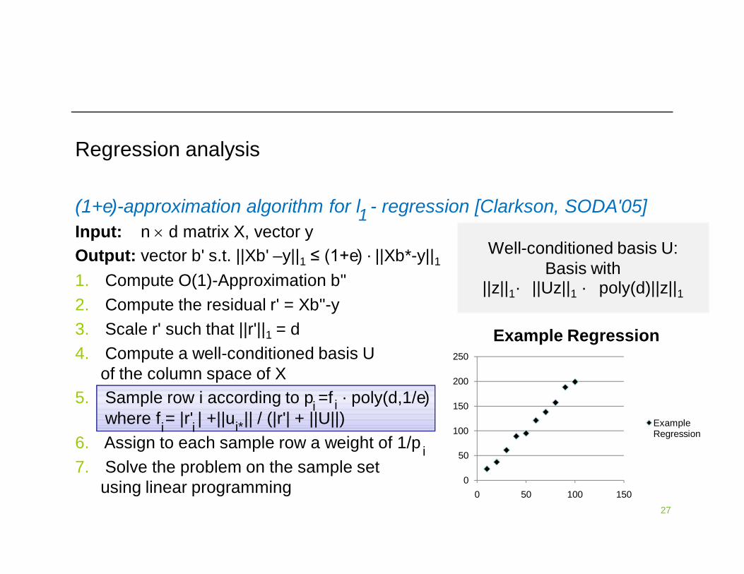
(1+e)-approximation algorithm for l - regression [Clarkson, SODA'05]Input: n d matrix X, vector yOutput: vector b' s.t. ||Xb' –y||1 ≤ (1+e) ∙ ||Xb*-y||11. Compute O(1)-Approximation b"2. Compute the residual r' = Xb"-y 3. Scale r' such that ||r'||1 = d4. Compute a well-conditioned basis U
of the column space of X5. Sample row i according to p =f ∙ poly(d,1/e)
where f = |r' | +||u || / (|r'| + ||U||)6. Assign to each sample row a weight of 1/p7. Solve the problem on the sample set
using linear programming
Well-conditioned basis U:Basis with
||z||1· ||Uz||1 · poly(d)||z||1
29
Regression analysis
1
i
ii
i*
i
i
0
50
100
150
200
250
0 50 100 150
Example Regression
Example Regression
(1+e)-approximation algorithm for l - regression [Clarkson, SODA'05]Input: n d matrix X, vector yOutput: vector b' s.t. ||Xb' –y||1 ≤ (1+e) ∙ ||Xb*-y||11. Compute O(1)-Approximation b"2. Compute the residual r' = Xb"-y 3. Scale r' such that ||r'||1 = d4. Compute a well-conditioned basis U
of the column space of X5. Sample row i according to p =f ∙ poly(d,1/e)
where f = |r' | +||u || / (|r'| + ||U||)6. Assign to each sample row a weight of 1/p7. Solve the problem on the sample set
using linear programming
Well-conditioned basis U:Basis with
||z||1· ||Uz||1 · poly(d)||z||1
30
Regression analysis
1
i
ii
i*
i
i
0
50
100
150
200
250
0 50 100 150
Example Regression
Example Regression
(1+e)-approximation algorithm for l - regression [Clarkson, SODA'05]Input: n d matrix X, vector yOutput: vector b' s.t. ||Xb' –y||1 ≤ (1+e) ∙ ||Xb*-y||11. Compute O(1)-Approximation b"2. Compute the residual r' = Xb"-y 3. Scale r' such that ||r'||1 = d4. Compute a well-conditioned basis U
of the column space of X5. Sample row i according to p =f ∙ poly(d,1/e)
where f = |r' | +||u || / (|r'| + ||U||)6. Assign to each sample row a weight of 1/p7. Solve the problem on the sample set
using linear programming
Well-conditioned basis U:Basis with
||z||1· ||Uz||1 · poly(d)||z||1
31
Regression analysis
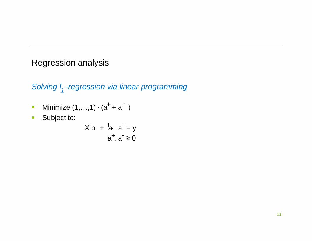
Solving l -regression via linear programming
Minimize (1,…,1) ∙ (a + a ) Subject to:
X b + a - a = ya , a ≥ 0
+ -
+ -
1
+ -
32
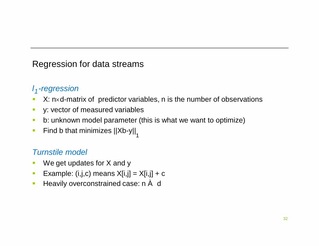
Regression for data streams
l -regression X: nd-matrix of predictor variables, n is the number of observations y: vector of measured variables b: unknown model parameter (this is what we want to optimize) Find b that minimizes ||Xb-y||
Turnstile model We get updates for X and y Example: (i,j,c) means X[i,j] = X[i,j] + c Heavily overconstrained case: n À d
1
1
33
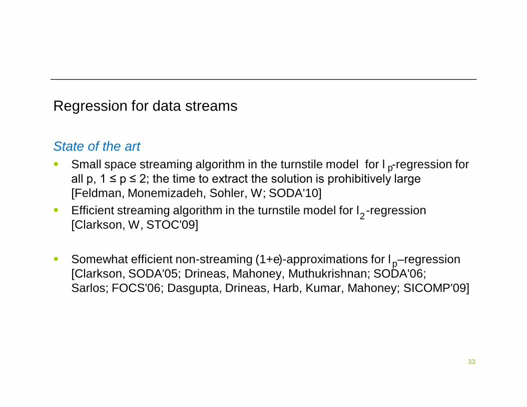
Regression for data streams
State of the art Small space streaming algorithm in the turnstile model for l -regression for
all p, 1 ≤ p ≤ 2; the time to extract the solution is prohibitively large[Feldman, Monemizadeh, Sohler, W; SODA'10]
Efficient streaming algorithm in the turnstile model for l -regression[Clarkson, W, STOC'09]
Somewhat efficient non-streaming (1+e)-approximations for l –regression[Clarkson, SODA'05; Drineas, Mahoney, Muthukrishnan; SODA'06; Sarlos; FOCS'06; Dasgupta, Drineas, Harb, Kumar, Mahoney; SICOMP'09]
p
2
p
34
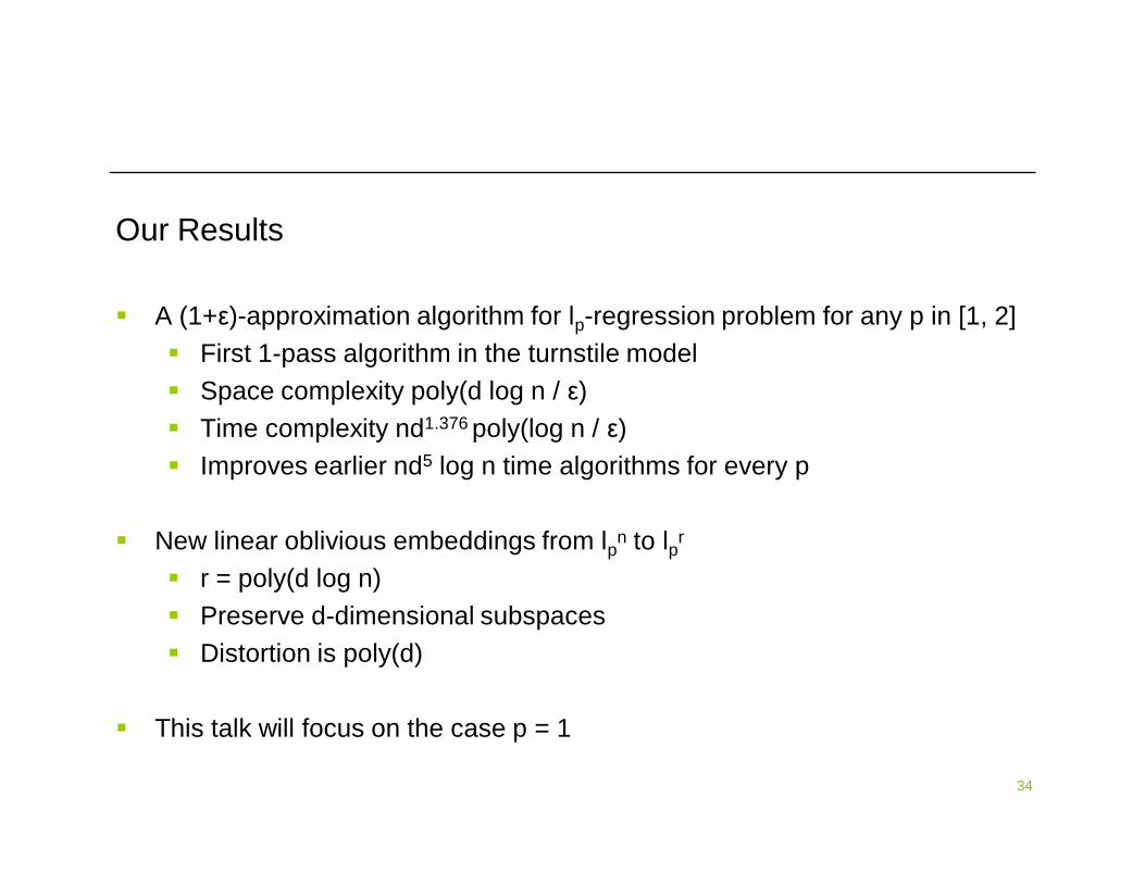
Our Results
A (1+ε)-approximation algorithm for lp-regression problem for any p in [1, 2] First 1-pass algorithm in the turnstile model Space complexity poly(d log n / ε) Time complexity nd1.376 poly(log n / ε) Improves earlier nd5 log n time algorithms for every p
New linear oblivious embeddings from lpn to lpr
r = poly(d log n) Preserve d-dimensional subspaces Distortion is poly(d)
This talk will focus on the case p = 1
35
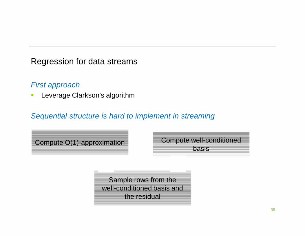
Regression for data streams
First approach Leverage Clarkson's algorithm
Sequential structure is hard to implement in streaming
Compute O(1)-approximation Compute well-conditionedbasis
Sample rows from the well-conditioned basis and
the residual
36
Regression for data streams
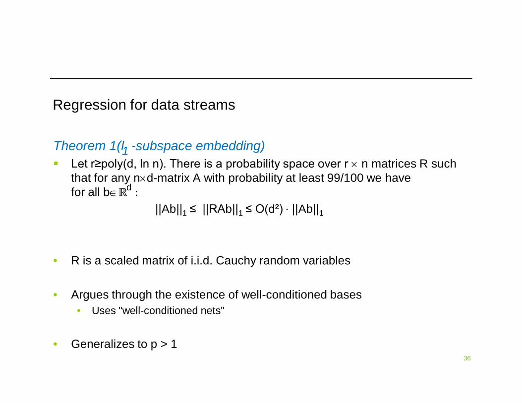
Theorem 1(l -subspace embedding) Let r≥poly(d, ln n). There is a probability space over r n matrices R such
that for any nd-matrix A with probability at least 99/100 we have for all bℝ :
||Ab||1 ≤ ||RAb||1 ≤ O(d²) ∙ ||Ab||1
• R is a scaled matrix of i.i.d. Cauchy random variables
• Argues through the existence of well-conditioned bases• Uses "well-conditioned nets"
• Generalizes to p > 1
d
1
37
Regression for data streams
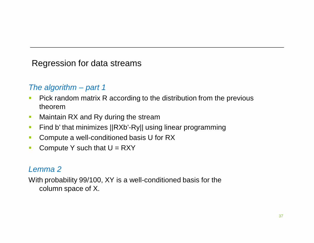
The algorithm – part 1 Pick random matrix R according to the distribution from the previous
theorem Maintain RX and Ry during the stream Find b' that minimizes ||RXb'-Ry|| using linear programming Compute a well-conditioned basis U for RX Compute Y such that U = RXY
Lemma 2With probability 99/100, XY is a well-conditioned basis for the
column space of X.
38
Regression for data streams
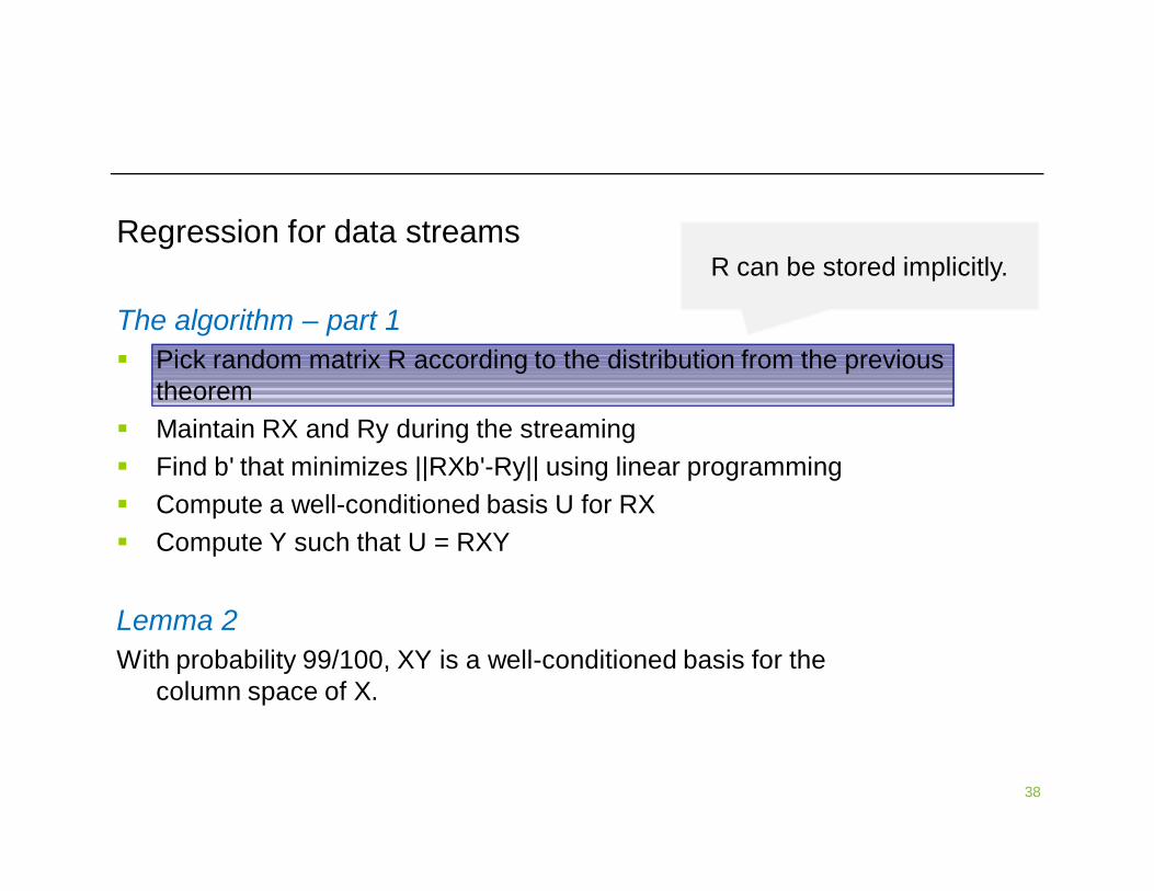
The algorithm – part 1 Pick random matrix R according to the distribution from the previous
theorem Maintain RX and Ry during the streaming Find b' that minimizes ||RXb'-Ry|| using linear programming Compute a well-conditioned basis U for RX Compute Y such that U = RXY
Lemma 2With probability 99/100, XY is a well-conditioned basis for the
column space of X.
R can be stored implicitly.
39
Regression for data streams
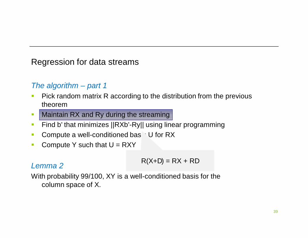
The algorithm – part 1 Pick random matrix R according to the distribution from the previous
theorem Maintain RX and Ry during the streaming Find b' that minimizes ||RXb'-Ry|| using linear programming Compute a well-conditioned basis U for RX Compute Y such that U = RXY
Lemma 2With probability 99/100, XY is a well-conditioned basis for the
column space of X.
R(X+D) = RX + RD
40
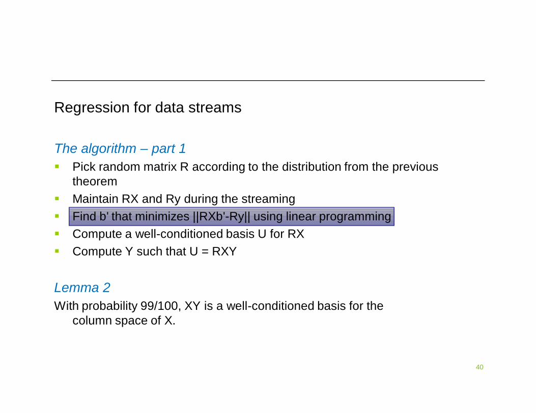
Regression for data streams
The algorithm – part 1 Pick random matrix R according to the distribution from the previous
theorem Maintain RX and Ry during the streaming Find b' that minimizes ||RXb'-Ry|| using linear programming Compute a well-conditioned basis U for RX Compute Y such that U = RXY
Lemma 2With probability 99/100, XY is a well-conditioned basis for the
column space of X.
41
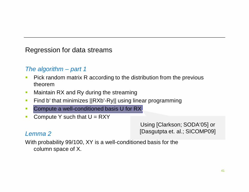
Regression for data streams
The algorithm – part 1 Pick random matrix R according to the distribution from the previous
theorem Maintain RX and Ry during the streaming Find b' that minimizes ||RXb'-Ry|| using linear programming Compute a well-conditioned basis U for RX Compute Y such that U = RXY
Lemma 2With probability 99/100, XY is a well-conditioned basis for the
column space of X.
Using [Clarkson; SODA‘05] or[Dasgutpta et. al.; SICOMP09]
42
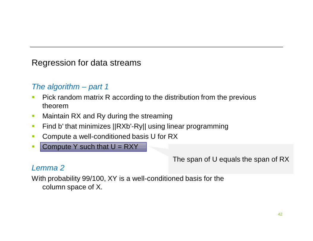
Regression for data streams
The algorithm – part 1 Pick random matrix R according to the distribution from the previous
theorem Maintain RX and Ry during the streaming Find b' that minimizes ||RXb'-Ry|| using linear programming Compute a well-conditioned basis U for RX Compute Y such that U = RXY
Lemma 2With probability 99/100, XY is a well-conditioned basis for the
column space of X.
The span of U equals the span of RX
43
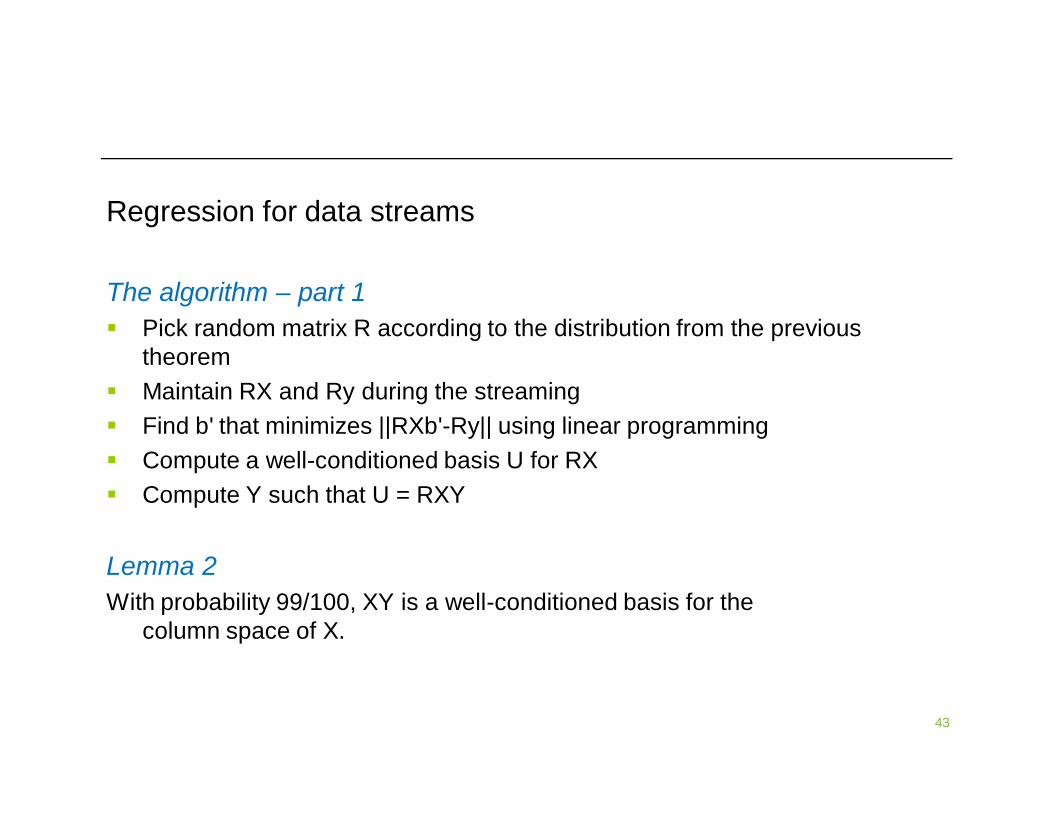
Regression for data streams
The algorithm – part 1 Pick random matrix R according to the distribution from the previous
theorem Maintain RX and Ry during the streaming Find b' that minimizes ||RXb'-Ry|| using linear programming Compute a well-conditioned basis U for RX Compute Y such that U = RXY
Lemma 2With probability 99/100, XY is a well-conditioned basis for the
column space of X.
44
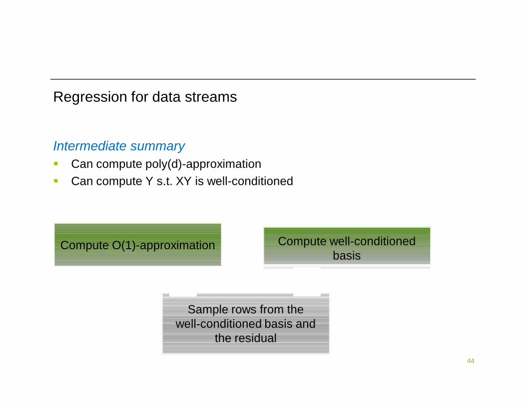
Regression for data streams
Intermediate summary Can compute poly(d)-approximation Can compute Y s.t. XY is well-conditioned
Compute O(1)-approximation Compute well-conditionedbasis
Sample rows from the well-conditioned basis and
the residual
45
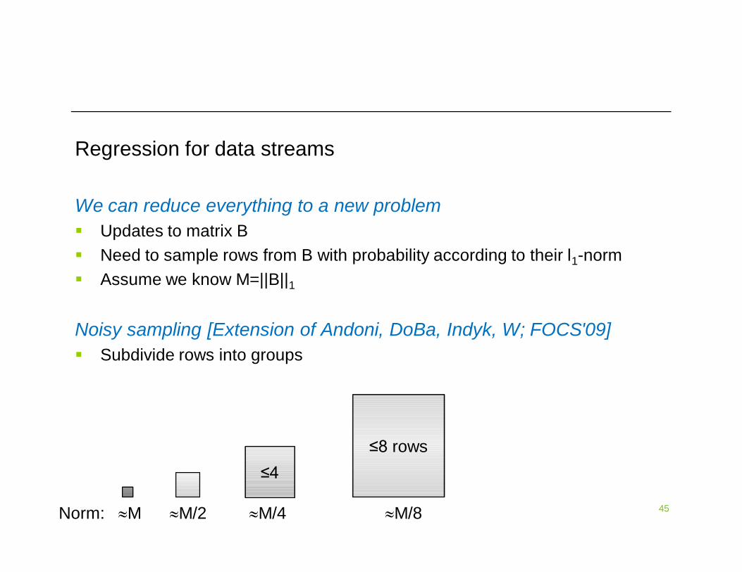
Regression for data streams
We can reduce everything to a new problem Updates to matrix B Need to sample rows from B with probability according to their l1-norm Assume we know M=||B||1
Noisy sampling [Extension of Andoni, DoBa, Indyk, W; FOCS'09] Subdivide rows into groups
≤4≤8 rows
Norm: M M/2 M/4 M/8
46
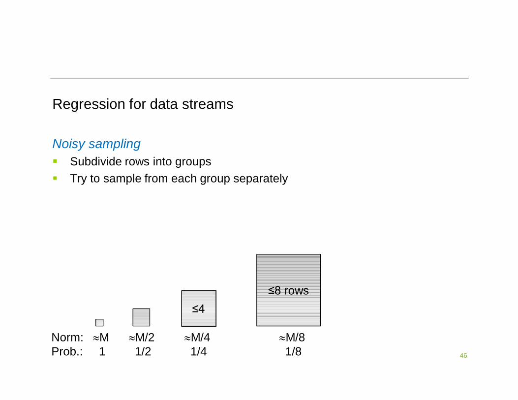
Regression for data streams
Noisy sampling Subdivide rows into groups Try to sample from each group separately
≤4≤8 rows
Norm: M M/2 M/4 M/8 Prob.: 1 1/2 1/4 1/8
47
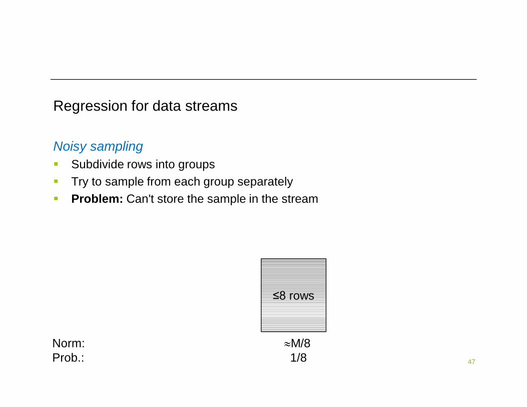
Regression for data streams
Noisy sampling Subdivide rows into groups Try to sample from each group separately Problem: Can't store the sample in the stream
≤8 rows
Norm: M/8Prob.: 1/8
48
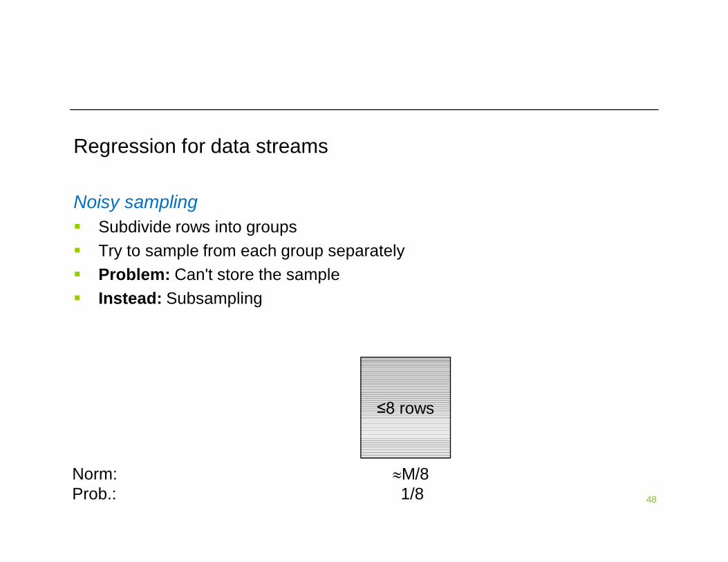
Regression for data streams
Noisy sampling Subdivide rows into groups Try to sample from each group separately Problem: Can't store the sample Instead: Subsampling
≤8 rows
Norm: M/8Prob.: 1/8
49
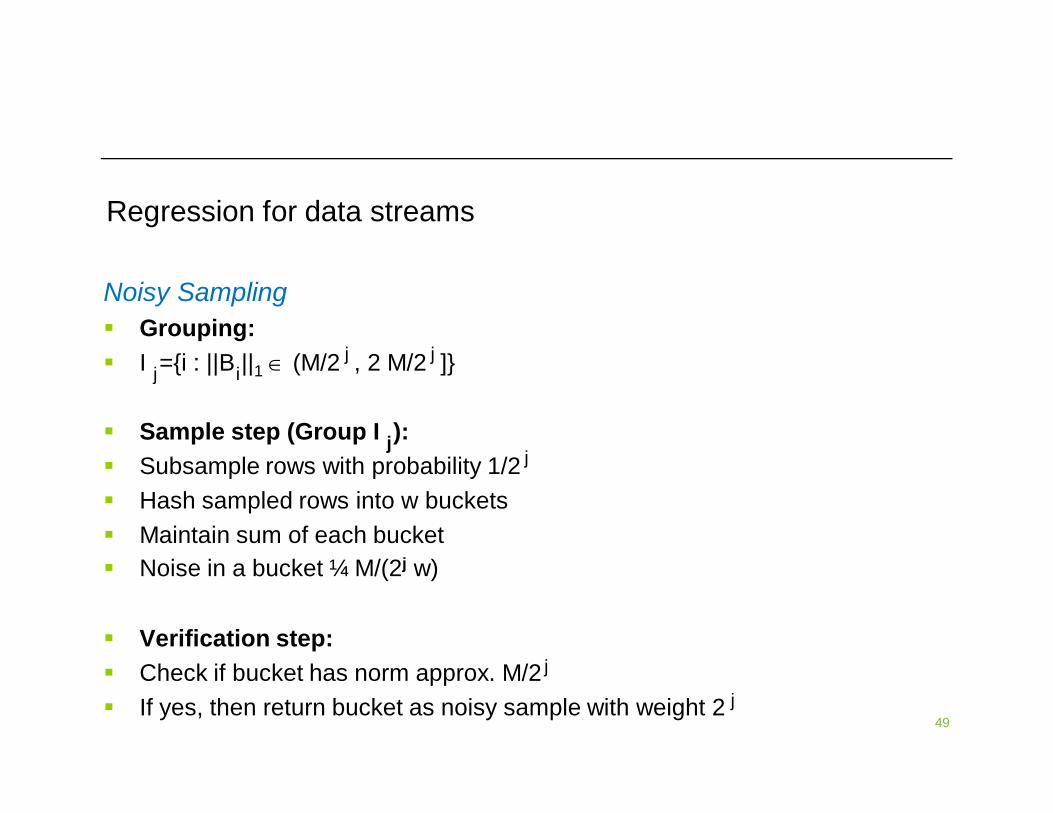
Regression for data streams
Noisy Sampling Grouping: I ={i : ||B ||1 (M/2 , 2 M/2 ]}
Sample step (Group I ): Subsample rows with probability 1/2 Hash sampled rows into w buckets Maintain sum of each bucket Noise in a bucket ¼ M/(2j w)
Verification step: Check if bucket has norm approx. M/2 If yes, then return bucket as noisy sample with weight 2
j ij j
jj
j
j
50
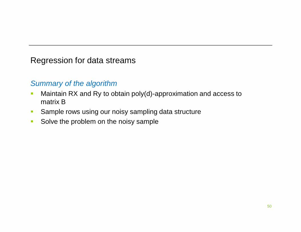
Regression for data streams
Summary of the algorithm Maintain RX and Ry to obtain poly(d)-approximation and access to
matrix B Sample rows using our noisy sampling data structure Solve the problem on the noisy sample
51
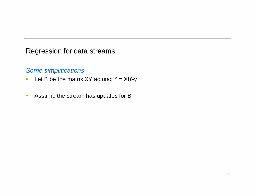
Regression for data streams
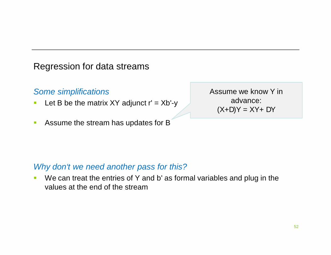
Some simplifications Let B be the matrix XY adjunct r' = Xb'-y
Assume the stream has updates for B
52
Regression for data streams
Some simplifications Let B be the matrix XY adjunct r' = Xb'-y
Assume the stream has updates for B
Why don‘t we need another pass for this? We can treat the entries of Y and b' as formal variables and plug in the
values at the end of the stream
Assume we know Y in advance:
(X+D)Y = XY+ DY
53
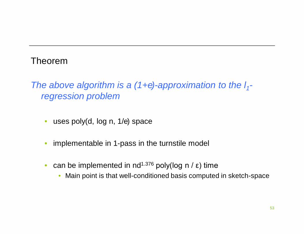
Theorem
The above algorithm is a (1+e)-approximation to the l1-regression problem
• uses poly(d, log n, 1/e) space
• implementable in 1-pass in the turnstile model
• can be implemented in nd1.376 poly(log n / ε) time• Main point is that well-conditioned basis computed in sketch-space
54
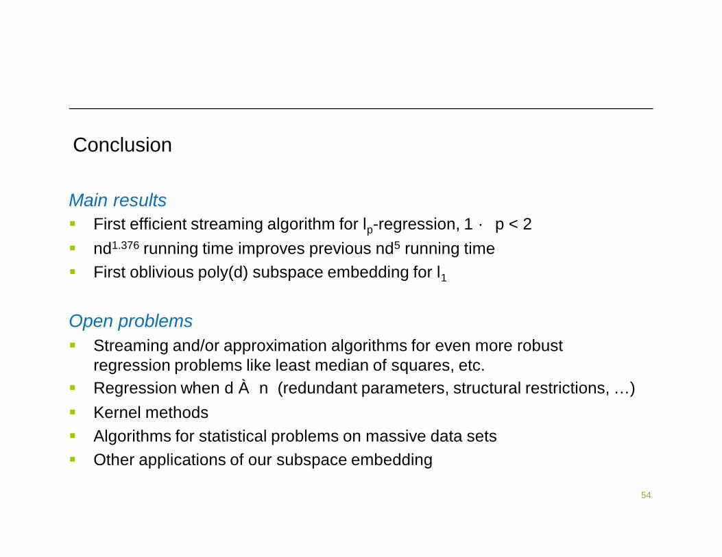
Conclusion
Main results First efficient streaming algorithm for lp-regression, 1 · p < 2 nd1.376 running time improves previous nd5 running time First oblivious poly(d) subspace embedding for l1
Open problems Streaming and/or approximation algorithms for even more robust
regression problems like least median of squares, etc. Regression when d À n (redundant parameters, structural restrictions, …) Kernel methods Algorithms for statistical problems on massive data sets Other applications of our subspace embedding
![arXiv:1911.04127v1 [cs.CV] 11 Nov 2019 · (DBG). DBG contains three modules: dual stream BaseNet (DSB), action-aware completeness regression (ACR) and temporal boundary classification](https://img.pdfslide.us/doc/110x75/5fed6515f032d014d24dfd1f/arxiv191104127v1-cscv-11-nov-2019-dbg-dbg-contains-three-modules-dual-stream.jpg)