Fast Greeks by algorithmic differentiation - Luca … · Fast Greeks by algorithmic differentiation 5 (or backward) mode is most efﬁcient in the more common situations where the

The Journal of Computational Finance (3–35) Volume 14/Number 3, Spring 2011

Fast Greeks by algorithmic differentiation

Luca CapriottiQuantitative Strategies, Investment Banking Division, Credit Suisse Group,Eleven Madison Avenue, New York, NY 10010-3086, USA;email: [email protected]

We show how algorithmic differentiation can be used to efficiently implement thepathwise derivative method for the calculation of option sensitivities using MonteCarlo simulations. The main practical difficulty of the pathwise derivative methodis that it requires the differentiation of the payout function. For the type of struc-tured options for which Monte Carlo simulations are usually employed, thesederivatives are typically cumbersome to calculate analytically, and too time con-suming to evaluate with standard finite-difference approaches. In this paper weaddress this problem and show how algorithmic differentiation can be employedto calculate these derivatives very efficiently and with machine-precision accu-racy. We illustrate the basic workings of this computational technique by means ofsimple examples, and we demonstrate with several numerical tests how the path-wise derivative method combined with algorithmic differentiation – especially inthe adjoint mode – can provide speed-ups of several orders of magnitude withrespect to standard methods.

1 INTRODUCTION

Monte Carlo simulations are becoming the main tool in the financial services industryfor pricing and hedging complex derivatives securities. In fact, as a result of the ever-increasing level of sophistication of the financial markets, a considerable fraction ofthe pricing models employed by investment firms is too complex to be treated by ana-lytic or deterministic numerical methods. For these models, Monte Carlo simulationis the only computationally feasible pricing technique.

It is a pleasure to acknowledge useful discussions and correspondence with Mike Giles, Paul Glasser-man, Laurent Hascoët, Jacky Lee, Jason McEwen, Adam and Matthew Peacock, Alex Prideaux andDavid Shorthouse. Special thanks are also due to Mike Giles for a careful reading of the manuscriptand valuable feedback. Constructive criticisms and suggestions by the two anonymous referees andthe associate editor are also gratefully acknowledged. The algorithmic differentiation codes used inthis paper were generated using Tapenade, developed at INRIA. The opinion and views expressedin this paper are those of the author alone and do not necessarily represent those of Credit SuisseGroup.

3

4 L. Capriotti

The main drawback of Monte Carlo simulations is that they are generally computa-tionally expensive. These efficiency issues become even more dramatic when MonteCarlo simulations are used for the calculation of the “Greeks”, or price sensitivities,which are necessary to hedge the financial risk associated with a derivative security.Indeed, the standard method for the calculation of the price sensitivities, also knownas “bumping”, involves perturbing the underlying model parameters in turn, repeat-ing the simulation and forming finite-difference approximations, thus resulting in acomputational burden increasing linearly with the number of sensitivities computed.This becomes very significant when the models employed depend on a large numberof parameters, as is typically the case for the sophisticated models for which MonteCarlo simulations are used in practice.

Alternative methods for the calculation of price sensitivities have been proposed inthe literature (for a review see, for example, Glasserman (2004)). Among these, thepathwise derivative method (Broadie and Glasserman (1996); Chen and Fu (2002);and Glasserman (2004)) provides unbiased estimates at a computational cost thatfor simple problems is generally smaller than that of bumping. The main limitationof the technique is that it involves the differentiation of the payout function. Thesederivatives are usually cumbersome to evaluate analytically, thus making the prac-tical implementation of the pathwise derivative method problematic. Of course, thepayout derivatives can always be approximated by finite-difference estimators. How-ever, this involves multiple evaluations of the payout function, and it is in generalcomputationally expensive.

A more efficient implementation of the pathwise derivative method was proposed ina remarkable paper by Giles and Glasserman (2006) for the LIBOR market model andEuropean-style payouts, and was recently generalized for simple Bermudan optionsby Leclerc et al (2009). The main advantage of this method is that it allows the calcu-lation of the price sensitivities at a greatly reduced price with respect to the standardimplementation. One drawback, as in the standard pathwise derivative method, is thatit involves the calculation of the derivatives of the payout function with respect to thevalue of the underlying market factors.

In this paper we illustrate how the problem of the efficient calculation of the deriva-tives of the payout can be overcome by using algorithmic differentiation (AD) (seeGriewank (2000)). Indeed, AD makes possible the automatic generation of efficientcoding implementing the derivatives of the payout function. In particular, the tangent(or forward) mode of AD is well suited for highly vectorized payouts depending on asmall number of observations of a limited number of underlying assets. This situationarises, for instance, when the same payout function with different parameters is usedto price several trades depending on the same (small) set of market observations, andthe sensitivities associated with each trade are required. On the other hand, the adjoint

The Journal of Computational Finance Volume 14/Number 3, Spring 2011

Fast Greeks by algorithmic differentiation 5

(or backward) mode is most efficient in the more common situations where the num-ber of observations of the underlying assets is larger than the number of securitiessimultaneously evaluated in the payout, or when interest lies in the aggregated risk ofa portfolio. In these cases, the implementation of the pathwise derivative method bymeans of the adjoint mode of AD – adjoint algorithmic differentiation (AAD) – canprovide speed-ups of several orders of magnitude with respect to standard methods.

In companion papers (Capriotti and Giles (2010) and Capriotti and Giles (2011)),we show howAAD can be used to efficiently implement not only the derivatives of thepayout function but also the so-called tangent state vector (see the next section). Thisallows us to make the ideas proposed in Giles and Glasserman (2006) completelygeneral and applicable to virtually any derivative or model commonly used in thefinancial industry.1

The remainder of this paper is organized as follows. In the next section, we set thenotation and briefly review the pathwise derivative method. The basic workings ofADare then introduced in Section 3 by means of simple examples. In Section 4 we discussin detail how AD can be used to generate efficient coding for the calculation of thederivatives of the payout function. Here we present numerical results comparing theefficiency of the tangent and adjoint modes as a function of the number of derivativescomputed. From this discussion it will be clear that, in most circumstances, the adjointmode is the one that is best suited when calculating the risk of complex derivatives.The computational efficiency of the pathwise derivative method with adjoint payoutsis discussed and tested with several numerical examples in Section 5. We draw theconclusions of this paper in Section 6.

2 THE PATHWISE DERIVATIVE METHOD

Option pricing problems can typically be formulated in terms of the calculation ofexpectation values of the form (Harrison and Kreps (1979)):

V D EQŒP.X.T1/; : : : ; X.TM //� (2.1)

Here X.t/ is an N -dimensional vector and represents the value of a set of under-lying market factors (stock prices, interest rates, foreign exchange pairs, etc) at timet . P.X.T1/; : : : ; X.TM // is the payout function of the priced security, and dependsin general on M observations of those factors. In the following, we will denotethe collection of such observations by a d D .N � M/-dimensional state vectorX D .X.T1/; : : : ; X.TM //

T, and by Q.X/ the appropriate risk-neutral distribution(Harrison and Kreps (1979)) according to which the components ofX are distributed.

1 The connection between AD and the adjoint approach of Giles and Glasserman (2006) is alsodiscussed in Giles (2007).

Research Paper www.journalofcomputationalfinance.com

6 L. Capriotti

The expectation value in (2.1) can be estimated by means of Monte Carloby sampling a number NMC of random replicas of the underlying state vectorXŒ1�; : : : ; XŒNMC�, sampled according to the distribution Q.X/, and evaluating thepayout P.X/ for each of them. This leads to the central limit theorem (Kallenberg(1997)) estimate of the option value V as:

V '1

NMC

NMCXiMCD1

P.XŒiMC�/ (2.2)

with standard error˙=pNMC, where˙2 D EQŒP.X/

2��EQŒP.X/�2 is the variance

of the sampled payout.The pathwise derivative method allows the calculation of the sensitivities of

the option price V (Equation (2.1)) with respect to a set of N� parameters � D.�1; : : : ; �N� /, with a single simulation. This can be achieved by noticing that, when-ever the payout function is regular enough (eg, Lipschitz continuous), and underadditional conditions that are often satisfied in financial pricing (see, for example,Glasserman (2004)), the sensitivity N�k � @V=@�k can be written as:

N�k D EQ

�@P� .X/

@�k

�(2.3)

In general, the calculation of Equation (2.3) can be performed by applying thechain rule, and averaging on each Monte Carlo path the so-called pathwise derivativeestimator:

N�k �@P� .X/

@�kD

dXjD1

@P� .X/

@Xj

@Xj

@�kC@P� .X/

@�k(2.4)

It is worth noting (although it is generally overlooked in the academic literature) thatthe payout P� .X.�// may depend on � not only implicitly through the vector X.�/,but also explicitly. The second term in Equation (2.4) is therefore important and needsto be kept in mind when implementing the pathwise derivative method.

The matrix of derivatives of each state variable in (2.4), or tangent state vector, isby definition given by:

@Xj

@�kD lim��!0

Xj .�1; : : : ; �k C��; : : : ; �N� / �Xj .�/

��(2.5)

This gives the intuitive interpretation of @Xj =@�k in terms of the difference betweenthe sample of the j th component of the state vector obtained after an infinitesimal“bump” of the kth parameter, Xj .�1; : : : ; �k C ��; : : : ; �N� /, and the base sampleXj .�/, both calculated on the same random realization.



In the special case in which the state vectorX D .X.T1/; : : : ; X.TM // is a path ofan N -dimensional diffusive process, the pathwise derivative estimator (2.4) may berewritten as:

N�k D

MXlD1

NXjD1

@P.X.T1/; : : : ; X.TM //

@Xj .Tl/

@Xj .Tl/

@�kC@P� .X/

@�k(2.6)

where we have relabeled the d components of the state vector X grouping togetherdifferent observationsXj .T1/; : : : ; Xj .TM / of the same (j th) asset. In particular, thecomponents of the tangent vector for the kth sensitivity corresponding to observationsat times .T1; : : : ; TM / along the path of the j th asset, say:

�jk.Tl/ D@Xj .Tl/

@�k(2.7)

with l D 1; : : : ;M , can be obtained by solving a stochastic differential equation(Kunita (1990); Protter (1997); and Glasserman (2004)).

The pathwise derivative estimators of the sensitivities are mathematically equiva-lent2 to the estimates obtained by bumping, using the same random numbers in bothsimulations, and for a vanishingly small perturbation. In fact, when using the sameset of random numbers for the base and bumped simulations of the expectation in(2.2), the finite-difference estimator of the kth sensitivity is equivalent to the averageover the Monte Carlo paths of the quantity:

P.X.� .k//ŒiMC�/ � P.X.�/ŒiMC�/

��(2.8)

with � .k/ D .�1; : : : ; �k C ��; : : : ; �N� /. In the limit �� ! 0, this is equivalentin turn to Equation (2.3). As a result, the pathwise derivative method and bumpingprovide in the limit �� ! 0 exactly the same estimators for the sensitivities, ie,estimators with the same expectation value, and the same Monte Carlo variance.

Since bumping and the pathwise derivative method provide estimates of the optionsensitivities with comparable variance, the implementation effort associated with thelatter is generally justified if the computational cost of the estimator (2.3) is less thanthe corresponding one associated with bumping.

The computational cost of evaluating the tangent state vector is strongly dependenton the problem considered. In some situations, its calculation can be implementedat a cost that is smaller than that associated with the propagation of the perturbedpaths in bumping. Apart from very simple models, this is the case, for instance, in the

2 Provided that the state vector is a sufficiently regular function of � (Glasserman (2004) and Protter(1997)).


8 L. Capriotti

examples considered by Glasserman and Zhao (1999) in the context of the LIBORmarket model.

However, when an efficient implementation of the tangent state vector is possible,the calculation of the gradient of the payout can constitute a significative part ofthe total computational cost, decreasing or eliminating altogether the benefits of thepathwise derivative method. Indeed, payouts of structured products often dependon hundreds of observations of several underlying assets, and their calculation isgenerally time consuming. For these payouts, the analytic calculation of the gradient isusually too cumbersome so that finite differences are the only practical route available(Giles and Glasserman (2006)). The multiple evaluation of the payout to obtain a largenumber of gradient components can by itself make the pathwise derivative methodless efficient than bumping.

The efficient calculation of the derivatives of the payout is therefore critical forthe successful implementation of the pathwise derivative method. In the following,we will illustrate how such an efficient calculation can be achieved by means ofAD. In particular, we will show that the adjoint mode of AD allows the gradientof the payout function to be obtained at a computational cost that is bounded byapproximately four times the cost of evaluating the payout itself, thus solving one ofthe main implementation difficulties – and performance bottlenecks – of the pathwisederivative method.

We will begin by reviewing the main ideas behind this powerful computationaltechnique in the next section.

3 ALGORITHMIC DIFFERENTIATION

Algorithmic differentiation is a set of programming techniques first introduced in theearly 1960s aimed at accurately and efficiently computing the derivatives of a functiongiven in the form of a computer program. The main idea underlying AD is that anysuch computer program can be interpreted as the composition of functions, each ofwhich is in turn a composition of basic arithmetic (addition, multiplication, etc), andintrinsic operations (logarithm, exponential, etc). Hence, it is possible to calculatethe derivatives of the outputs of the program with respect to its inputs by applyingmechanically the rules of differentiation. This makes it possible to generate auto-matically a computer program that evaluates efficiently and with machine-precisionaccuracy the derivatives of the function (Griewank (2000)).

What makes AD particularly attractive when compared to standard (eg, finite-difference) methods for the calculation of the derivatives is its computational effi-ciency. In fact, AD aims to exploit the information on the structure of the computerfunction, and on the dependencies between its various parts, in order to optimize thecalculation of the sensitivities.



In the following, we will review these ideas in more detail. In particular, we willdescribe the two basic approaches toAD, the so-called tangent (or forward) and adjoint(or backward) modes. These differ in regard to how the chain rule is applied to thecomposition of instructions representing a given function, and are characterized bydifferent computational costs for a given set of computed derivatives. Griewank (2000)contains a complete introduction to AD. Here, we will only recall the main results inorder to clarify how this technique is beneficial in the implementation of the pathwisederivative method. We will begin by stating the results regarding the computationalefficiency of the two modes of AD, and we will justify them by discussing a toyexample in detail.

3.1 Computational complexity of the tangent and adjoint modes ofalgorithmic differentiation

Let us consider a computer program with n inputs, x D .x1; : : : ; xn/ and m outputsy D .y1; : : : ; ym/ that is defined by a composition of arithmetic and nonlinear (intrin-sic) operations. Such a program can be seen as a function of the form F W Rn ! Rm:

.y1; : : : ; ym/T D F.x1; : : : ; xn/ (3.1)

In its simplest form, AD aims to produce coding evaluating the sensitivities of theoutputs of the original program with respect to its inputs, ie, to calculate the Jacobianof the function F :

Jij D@Fi .x/

@xj(3.2)

with Fi .x/ D yi .The tangent mode ofAD allows the calculation of the functionF and of its Jacobian

at a cost – relative to that for F – that can be shown, under a standard computationalcomplexity model (Griewank (2000)), to be bounded by a small constant, !T , timesthe number of independent variables, namely:

CostŒF& J �

CostŒF �6 !T n (3.3)

The value of the constant !T can be also bounded using a model of the relative costof algebric operations, nonlinear unary functions and memory access. This analysisgives !T 2 Œ2; 52 � (Griewank (2000)).

The form of the result (3.3) appears quite natural as it is the same computationalcomplexity of evaluating the Jacobian by perturbing one input variable at a time,repeating the calculation of the function, and forming the appropriate finite-differenceestimators. As we will illustrate in the next section, the tangent mode avoids repeating


10 L. Capriotti

the calculations of quantities that are left unchanged by the perturbations of the dif-ferent inputs, and it is therefore generally more efficient than bumping.

Consistent with Equation (3.3), the tangent mode of AD provides the derivativesof all the m components of the output vector y with respect to a single input xj , ie,a single column of the Jacobian (3.2), at a cost that is independent of the number ofdependent variables and bounded by a small constant, !T . In fact, the same holdstrue for any linear combination of the columns of the Jacobian, Lc.J /, namely:

CostŒF& Lc.J /�

CostŒF �6 !T (3.4)

This makes the tangent mode particularly well suited for the calculation of (linearcombinations of) the columns of the Jacobian matrix (3.2). Conversely, it is generallynot the method of choice for the calculation of the gradients (ie, the rows of theJacobian (3.2)) of functions of a large number of variables.

On the other hand, the adjoint mode of AD, or AAD, is characterized by a compu-tational cost of the form (Griewank (2000)):

CostŒF& J �

CostŒF �6 !Am (3.5)

with !A 2 Œ3; 4�, ie, AAD allows the calculation of the function F and of its Jacobianat a cost – relative to that forF – that is bounded by a small constant times the numberof dependent variables.

As a result,AAD provides the full gradient of a scalar (m D 1) function at a cost thatis just a small constant, times the cost of evaluating the function itself. Remarkably,such relative cost is independent of the number of components of the gradient.

For vector-valued functions, AAD provides the gradient of arbitrary linear combi-nations of the rows of the Jacobian, Lr.J /, at the same computational cost as for asingle row, namely:

CostŒF& Lr.J /�

CostŒF �6 !A (3.6)

This clearly makes the adjoint mode particularly well suited for the calculation of(linear combinations of) the rows of the Jacobian matrix (3.2). When the full Jacobianis required, the adjoint mode is likely to be more efficient than the tangent modewhen the number of independent variables is significantly larger than the number ofdependent ones (m� n).

We now provide justification of these results by discussing an explicit example indetail.



3.2 How algorithmic differentiation works: a simple example

Let us consider, as a specific example, the function F W R2 ! R3, .y1; y2/T D.F1.x1; x2; x3/; F2.x1; x2; x3//

T defined as: y1

y2

!D

2 log x1x2 C 2 sin x1x2

4 log2 x1x2 C cos x1x3 � 2x3 � x2

!(3.7)

3.2.1 Algorithmic specification of functions and computational graphs

Given a value of the input vector x, the output vector y is calculated by a computercode by means of a sequence of instructions. In particular, the execution of the programcan be represented in terms of a set of scalar internal variables, w1; : : : ; wN , suchthat:

wi D xi ; i D 1; : : : ; n (3.8)

wi D ˚i .fwj gj�i /; i D nC 1; : : : ; N (3.9)

Here the first n variables are copies of the input ones, and the others are given by asequence of consecutive assignments; the symbol fwj gj�i indicates the set of internalvariables wj , with j < i , such that wi depends explicitly on wj ; the functions˚i represent a composition of one or more elementary or intrinsic operations. Inthis representation, the last m internal variables are the output of the function, ie,yi�NCm D wi , i D N �mC 1; : : : ; N . This representation is by no means unique,and can be constructed in a variety of ways. However, it is a useful abstraction in orderto introduce the mechanism of AD. For instance, for the function (3.7), the internalcalculations can be represented as follows:

w1 D x1; w2 D x2; w3 D x3

#

w4 D ˚4.w1; w2/ D 2 logw1w2

w5 D ˚5.w1; w2/ D 2 sinw1w2

w6 D ˚6.w1; w3/ D cosw1w3

w7 D ˚7.w2; w3/ D 2w3 C w2

#

y1 D w8 D ˚8.w4; w5/ D w4 C w5

y2 D w9 D ˚9.w4; w6; w7/ D w24 C w6 � w7

9>>>>>>>>>>>>>>>>>=>>>>>>>>>>>>>>>>>;

(3.10)

In general, a computer program contains loops that may be executed a fixed or variablenumber of times, and internal controls that alter the calculations performed according


12 L. Capriotti

FIGURE 1 Computational graph corresponding to the instructions (3.10) for the functionin Equation (3.7).

Out

y1 = w8 = w4 + w5

w4 = 2logw1w2

w1 = x1 w2 = x2 w3 = x3

w5 = 2sinw1w2 w6 = cosw1w3 w7 = 2w3 + w2

D8,4

D4,1

D4,2 D5,1

D6,1

D5,2

D7,2

D7,3D6,3

In

D8,5D9,4

D9,6 D9,7

y2 = w9 = w 24 + w6 – w7

to different criteria. Nevertheless, Equations (3.8) and (3.9) are an accurate represen-tation of how the program is executed for a given value of the input vector x, ie, for agiven instance of the internal controls. In this respect, AD aims to perform a piecewisedifferentiation of the program by reproducing the same controls in the differentiatedcode (Griewank (2000)).

The sequence of instructions (3.8) and (3.9) can be effectively represented bymeans of a computational graph with nodes given by the internal variables wi , andconnecting arcs between explicitly dependent variables. For instance, for the functionin Equation (3.7) the instructions (3.10) can be represented as in Figure 1. Moreover,to each arc of the computational graph, say connecting node wi and wj with j < i ,it is possible to associate the arc derivative:

Di;j D@˚i .fwkgk�i /

@wj(3.11)

as illustrated in Figure 1. Crucially, these derivatives can be calculated in an auto-matic fashion by applying mechanically the rules of differentiation instruction byinstruction.



3.2.2 Tangent mode

Once the program implementing F.x/ is represented in terms of the instructionsin (3.8) and (3.9) (or by a computational graph like that in Figure 1 on the facingpage) the calculation of the gradient of each of its m components:

rFi .x/ D .@x1Fi .x/; @x2Fi .x/; : : : ; @xnFi .x//T (3.12)

simply involves the application of the chain rule of differentiation. In particular, byapplying the rule starting from the independent variables, the tangent mode of AD isobtained:

rwi D ei ; i D 1; : : : ; n (3.13)

rwi DXj�i

Di;jrwj ; i D nC 1; : : : ; N (3.14)

where e1; e2; : : : ; en are the vectors of the canonical basis in Rn, and Di;j are thelocal derivatives (3.11). For the example in Equation (3.7) this gives, for instance:

rw1 D .1; 0; 0/T; rw2 D .0; 1; 0/

T; rw3 D .0; 0; 1/T

#

D4;1 D 2w2=.w1w2/; D4;2 D 2w1=.w1w2/

rw4 D D4;1rw1 CD4;2rw2

D5;1 D 2w2 cosw1w2; D5;2 D 2w1 cosw1w2


D6;1 D �w3 sinw1w3; D6;3 D �w1 sinw1w3


D7;2 D 1; D7;3 D 2

rw7 D D7;2 rw2 CD7;3rw3

#

D8;4 D 1; D8;5 D 1

ry1 D rw8 D D8;4rw4 CD8;5rw5

D9;4 D 2w4; D9;6 D 1; D9;7 D �1

ry2 D rw9 D D9;4rw4 CD9;6rw6 CD9;7rw7

This leads to:

ry1 D .D8;4D4;1 CD8;5D5;1;D8;4D4;2 CD8;5D5;2; 0/T

ry2 D .D9;4D4;1 CD9;6D6;1;D9;4D4;2

CD9;7D7;2;D9;6D6;3 CD9;7D7;3/T

which gives the correct result, as can immediately be verified.


14 L. Capriotti

In the relations above, each component of the gradient is propagated independently.As a result, the computational cost of evaluating the Jacobian of the function Fis approximately n times the cost of evaluating one of its columns, or any linearcombination of them. For this reason, the propagation in the tangent mode is moreconveniently expressed by replacing the vectors rwi with the scalars:

Pwi D

nXjD1

�j@wi

@xj(3.15)

also known as tangents. Here � is a vector in Rn specifying the chosen linear com-bination of columns of the Jacobian. Indeed, in this notation, the propagation of thechain rule (3.13) and (3.14) becomes:

Pwi D �i ; i D 1; : : : ; n (3.16)

Pwi DXj�i

Di;j Pwj ; i D nC 1; : : : ; N (3.17)

At the end of the propagation we therefore find Pwi , i D N �mC 1; : : : ; N :

Pwi D Pyi�NCm D

nXjD1

�j@wi

@xjD

nXjD1

�j@yi�NCm

@xj(3.18)

ie, a linear combination of the columns of the Jacobian.As illustrated in Figure 2 on the facing page, the propagation of the chain rule

(3.16) and (3.17) allows us to associate the tangent of the corresponding internalvariable, say Pwi , with each node of the computational graph. This can be calculatedas a weighted average of the tangents of the variables preceding it on the graph (ie,all the Pwj such that i � j ), with weights given by the arc derivatives associated withthe connecting arcs. As a result, the tangents propagate through the computationalgraph from the independent variables to the dependent ones, ie, in the same directionfollowed in the evaluation of the original function, or forward. The propagation ofthe tangents can in fact proceed instruction by instruction, at the same time as thefunction is evaluated.

It is easy to realize that the cost for the propagation of the chain rule (3.16) and(3.17), for a given linear combination of the columns of the Jacobian, is of the sameorder as the cost of evaluating the function F itself. Hence, for the simple exampleconsidered here, Equation (3.4) represents an appropriate estimate of the compu-tational cost of any linear combination of columns of the Jacobian. On the otherhand, in order to get each column of the Jacobian it is necessary to repeat n D 3

times the calculation of the computational graph in Figure 2 on the facing page,eg, by setting � equal to each vector of the canonical basis in R3. As a result, the



FIGURE 2 Computational graph for the tangent mode differentiation of the function inEquation (3.7).

Out

In

D8,4

D4,1

x1 = w1 = λ1 x2 = w2 = λ2

D4,2 D5,1

D6,1

D5,2D6,3

D7,2

D7,3

D8,5D9,4

D9,6 D9,7

D8,4w4 + D8,5w5⋅ ⋅

y1 = w8 ⋅ ⋅

w4 = D4,1w1 + D4,2w2

⋅ ⋅ ⋅ ⋅ x3 = w3 = λ3⋅ ⋅

w5 = D5,1w1 + D5,2w2⋅⋅ ⋅⋅⋅⋅ w6 = D6,1w1 + D6,3w3 w7 = D7,2w2 + D7,3w3

⋅⋅ ⋅ ⋅ ⋅⋅

D9,4w4 + D9,6 w6 + D9,7w7⋅ ⋅⋅

⋅ ⋅y2 = w9

==

computational cost of evaluating the Jacobian relative to the cost of evaluating thefunction F is proportional to the number of independent variables, as predicted byEquation (3.3).

Finally, we remark that, by simultaneously carrying out the calculation of all thecomponents of the gradient (or, more generally, of a set of n linear combinationsof columns of the Jacobian) the calculation can be optimized by reusing a certainamount of computations (eg, the arc derivatives). This leads to a more efficient imple-mentation also known as tangent multimode. Although the computational cost forthe tangent multimode remains of the form (3.3) and (3.4), the constant !T for theseimplementations is generally smaller than for the standard tangent mode. This willalso be illustrated in Section 4.

3.2.3 Adjoint mode

The adjoint mode provides the Jacobian of a function in a mathematically equivalentway by means of a different sequence of operations. More precisely, the adjoint mode


16 L. Capriotti

results from propagating the derivatives of the final result with respect to all theintermediate variables – the so-called adjoints – until the derivatives with respectto the independent variables are formed. Formally, the adjoint of any intermediatevariable wi is defined as:

Nwi D

mXjD1

�j@yj

@wi(3.19)

where � is a vector in Rm. In particular, for each of the dependent variables we haveNyi D �i , i D 1; : : : ; m, while, for the intermediate variables, we instead have:

Nwi D@y

@wiDXj�i

@y

@wj

@wj

@wiDXj�i

Dj;i Nwj (3.20)

where the sum is over the indices j > i such that wj depends explicitly on wi . Atthe end of the propagation we therefore find Nwi , i D 1; : : : ; n:

Nwi D Nxi D

mXjD1

�j@yj

@wiD

mXjD1

�j@yj

@xi(3.21)

ie, a given linear combination of the rows of the Jacobian (3.2).In particular, for the example in Equation (3.7) this gives:

Nw8 D Ny1 D �1; Nw9 D Ny2 D �2

#

Nw4 D D8;4 Nw8 CD9;4 Nw9

Nw5 D D8;5 Nw8

Nw6 D D9;6 Nw9

Nw7 D D9;7 Nw9

#

Nw1 D Nx1 D D4;1 Nw4 CD5;1 Nw5 CD6;1 Nw6

Nw2 D Nx2 D D4;2 Nw4 CD5;2 Nw5 CD7;2 Nw7

Nw3 D Nx3 D D6;3 Nw6 CD7;3 Nw7

It is immediately evident that, by setting � D e1 and � D e2 (with e1 and e2 canonicalvectors in R2), the adjoints . Nw1; Nw2; Nw3/ above give the components of the gradientsof ry1 and ry2, respectively.

As illustrated in Figure 3 on the facing page, Equation (3.20) has a clear interpre-tation in terms of the computational graph: the adjoint of a quantity on a given node,Nwi , can be calculated as a weighted sum of the adjoints of the quantities that depend

on it (ie, all the Nwj such that j � i ), with weights given by the local derivatives



FIGURE 3 Computational graph for the adjoint mode differentiation of the function inEquation (3.7).

Out

In

y1 = w8 = λ1–

y2 = w9 = λ2– –

D8,4

D4,1

D5,1w5 + D6,1w6– –

– ––x1 = w1 = D4,1w4+

D5,2w5 + D7,2w7– –

– ––x2 = w2 = D4,2w4 +

D6,3w6 + D7,3w7– –

––x3 = w3 =

D4,2 D5,1

D5,2

D6,1

D8,5

D9,4D9,6 D9,7

D7,2

D6,3 D7,3

– –w5 = D8,5w8– –w6 = D9,6w9

– –w7 = D9,7w9w4 = D8,4w8 + D9,4w9– – –

–

associated with the respective arcs. As a result, the adjoints propagate through thecomputational graph from the dependent variables to the independent ones, ie, in theopposite direction to that of evaluation of the original function, or backward. Themain consequence of this is that, in contrast to the tangent mode, the propagationof the adjoints cannot in general be simultaneous with the execution of the function.Indeed, the adjoint of each node depends on variables that are yet to be determinedon the computational graph. As a result, the propagation of the adjoints can in generalbegin only after the construction of the computational graph has been completed, andthe information on the values and dependences of the nodes on the graph (eg, the arcderivatives) has been appropriately stored.

It is easy to see that the cost for the propagation of the chain rule (3.20) for agiven linear combination of the rows of the Jacobian is of the same order as thecost of evaluating the function F itself, in agreement with Equation (3.6). On theother hand, in order to get each row of the Jacobian, m D 2 times the calculation


18 L. Capriotti

of the computational graph in Figure 3 on the preceding page has to be repeated,eg, by setting � equal to each vector of the canonical basis in R2. As a result, thecomputational cost of evaluating the Jacobian relative to the cost of evaluating thefunction F itself is proportional to the number of dependent variables, as predictedby Equation (3.5).

3.3 Algorithmic differentiation tools

As illustrated in the previous examples, AD gives a clear set of prescriptions bywhich, given any computer function, the code implementing the tangent or adjointmode for the calculation of its derivatives can be developed. This involves representingthe computer function in terms of its computational graph, calculating the derivativesassociated with each of the elementary arcs, and propagating either the tangents or theadjoints in the appropriate direction. This procedure, being mechanical in nature, canbe automated. Indeed, several AD tools have been developed that allow the automaticimplementation of the calculation of derivatives either in the tangent or in the adjointmode. These tools can be grouped into two main categories, namely source codetransformation and operator overloading.3

Source code transformation tools are computer programs that take the source codeof a function as input, and return the source code implementing its derivatives. Thesetools rely on parsing the instructions of the input code and constructing a representa-tion of the associated computational graph. In particular, an AD parser typically splitseach instruction into the constituent unary or binary elementary operations for whichthe corresponding derivative functions are known.

On the other hand, the operator overloading approach exploits the flexibility ofobject-oriented languages in order to introduce new abstract data types suitable forrepresenting tangents and adjoints. Standard operations and intrinsic functions arethen defined for the new types in order to allow the calculation of the tangents and theadjoints associated with any elementary instruction in a code. These tools operate bylinking a suitable set of libraries to the source code of the function to be differentiated,and by redefining the type of the internal variables. Utility functions are generallyprovided to retrieve the value of the desired derivatives.

Source code transformation and operator overloading are both the subject of activeresearch in the field of AD. Operator overloading is appealing for the simplicity ofusage that boils down to linking some libraries, redefining the types of the variables,and calling some utility functions to access the derivatives. The main drawback is thelack of transparency, and the fact that the calculation of derivatives is generally slowerthan in the source code transformation approach. Source code transformation involvesmore work but it is generally more transparent as it provides the code implementing the

3 An excellent source of information in the field can be found at www.autodiff.org.



calculation of the derivatives as a sequence of elementary instructions. This simplicityfacilitates compiler optimization, thus generally resulting in a faster execution. In thefollowing section we consider examples of the source code transformation approachwhile discussing the calculation of the derivatives of the payout required for theimplementation of the pathwise derivative method.

4 CALCULATING THE DERIVATIVES OF PAYOUT FUNCTIONSUSING ALGORITHMIC DIFFERENTIATION

In this section we discuss a few examples illustrating how AD can be used to produceefficient coding for the calculation of the derivatives of the payout in (2.4).

Payouts of structured products are typically scalar functions of a large numberof dependent variables. As a result, the adjoint mode of AD is generally best suitedfor the fast calculation of their derivatives. This will be clear from the examplesdiscussed in Section 4.1. On the other hand, for vector-valued payouts, the adjointand tangent modes of AD can often be combined in order to generate a highly efficientimplementation, as discussed in Section 4.2. As specific examples, in the followingwe will consider European-style basket options and path-dependent “best of” Asianoptions.

4.1 Scalar payouts

4.1.1 Basket options

In Figure 4 on the next page we show the pseudocode for the payout function and itsadjoint counterpart for a simple basket call option with payout:

P D Pr.X.T // D e�rT� NXiD1

wiXi .T / �K

�C(4.1)

where X.T / D .X1.T /; : : : ; XN .T // represent the value of a set of N underlyingassets at time T , say a set of equity prices, wi , i D 1; : : : ; n, are the weights definingthe composition of the basket,K is the strike price and r is the risk-free yield for thematurity considered. Here, for simplicity, we consider the case in which interest ratesare deterministic. As a result, the interest rate r can be seen as a model parameterdetermined by the yield curve. For this example, we are interested in the calculationof the sensitivities with respect to r and the N components of the state vector X sothat the other parameters (ie, strike and maturity) are seen here as dummy constants.

As illustrated in the pseudocode in part (a) of Figure 4 on the next page, theinputs of the computer function implementing the payout (4.1) are a scalar r andan N -dimensional vector X (we suppress the dependence on T from now on). The


20 L. Capriotti

FIGURE 4 Pseudocode for (a) the payout function and (b) its adjoint for the basket calloption of Equation (4.1).

(a)

(b)

output is a scalar P . On the other hand, the adjoint of the payout function, shown inpart (b) of Figure 4, is of the form:

.P; Nr; NX/ D NPr.X; NP / (4.2)

ie, it has the scaling factor NP as an additional scalar input, and the adjoints:

Nr [email protected]/

@rNP (4.3)

NXi [email protected]/

@XiNP (4.4)

for i D 1; : : : ; N as additional outputs. In this and in the following figures we use thesuffixes “_b” and “_d” to represent in the pseudocodes the “bar” and “dot” notationsfor adjoint and tangent quantities, respectively.



As discussed in Section 3, the adjoint payout function typically contains an initialforward sweep. This replicates the original payout script and evaluates the first outputP of the function.The forward sweep is also used to keep a record of all the informationnecessary to calculate the arc derivatives (Section 3.2.1) that cannot be recoveredefficiently going backwards on the computational graph. However, in this simpleexample, as shown in Figure 4 on the facing page, no information needs to be storedduring the forward sweep, and the latter is just an exact replica of the original payoutcode.

Once the forward sweep is completed, the backward sweep propagates the adjointquantities, reversing the order of the computations with respect to the original function.In the specific example, first the reverse sweep computes the adjoint counterpart ofthe very last instruction of the forward sweep:

P.D; x/ D D.x/C (4.5)

as seen as a function of the intermediate variables D and x. The adjoints of D and xare simply:

ND [email protected]; x/

@DNP D .x/C NP (4.6)

and:

Nx [email protected]; x/

@xNP D D#.x/ NP (4.7)

where #.x/ is the Heaviside function. Then, taking the adjoint of the functionD D exp.�rT / with constant T gives:

Nr [email protected]/

@rND D �DT ND (4.8)

Finally, the adjoint of the instructions x D x.B/ D B �K (with K constant) and:

B D B.X/ D

NXiD1

wiXi .T /

are computed in turn. Respectively, these are:

NB [email protected]/

@BNx D Nx (4.9)

and:NXi D

@B.X/

@XiNB D wi NB (4.10)

for i D 1; : : : ; N . It is easy to recognize that the quantities Nr and NX constructed thisway represent the adjoints in Equations (4.3) and (4.4), respectively. For NP D 1, theseclearly give the gradient of the payout function (4.1).


22 L. Capriotti

FIGURE 5 Ratios of the processing time required for the calculation of the value and of allthe derivatives of the payout function, and the processing time spent on the computationof its value alone, as functions of the number of assets, N .

0

0

20

10

0

50

CP

U r

atio

sC

PU

rat

ios

100

150

5 10 15 20

0 5 10 15 20N

~2.5

~1.7

(b)

(a)

(a) “Best of” Asian option (4.12) forM D 20 observation times. (b) Basket option (4.1). Symbols: triangles, tangent;stars, tangent multimode; circles, adjoint. The dotted line represents the estimated CPU ratios associated with one-sided finite differences. The other lines are guides for the eye.



FIGURE 6 Pseudocode for the tangent payout function for the basket call option ofEquation (4.1).

As mentioned in Section 3, AD cannot generally be expected to provide any mean-ingful results for those values of the input variables for which the function is notdifferentiable. This is the case, for instance, when the payout function involves themaximum function as in the example above. In this case, the derivatives for the setof inputs such that B.X/ D K are not defined, and are returned instead as zero.However, in the context of the pathwise derivative method, this does not create anypractical difficulty as the set of points corresponding to these singularity constitutesa zero probability subset of the sample space in Equation (2.1). In any case, it is alsogenerally possible to smooth out such singularities along the lines of the discussionin Section 4.3.

By inspecting the structure of the adjoint payout, it appears clear that its computa-tional cost is just a small multiple (of order two) of the cost of evaluating the originalpayout. Indeed, it is easy to realize that the cost of the forward and backward sweepsare roughly the same, thus making the cost of calculating the complete gradient of thepayout roughly twice the cost of evaluating the payout alone. In particular, the ratio ofthe processing time spent in the calculation of the adjoint payout and the processingtime spent in the original payout function is independent of the number of inputs, inagreement with Equation (3.6).

The remarkable efficiency of the adjoint payout function is clearly illustrated inpart (b) of Figure 5 on the facing page where the processing time ratio is plotted asa function of the number of assets N : the calculation of Nd D N C 1 derivativesof the payout (one for each asset plus the derivative with respect to r) requires an


24 L. Capriotti

FIGURE 7 Pseudocode for the tangent multimode payout function for the basket calloption of Equation (4.1).

extra overhead of about 70% with respect to the calculation of the payout itself forany number of underlying assets N . This is in stark contrast to the relative cost ofevaluating the gradient by means of one-sided finite differences or the tangent modeof AD (also shown in the same figure), both scaling linearly with N .

The pseudocodes for the tangent payout, in the standard and in the multimodeimplementation, are given in Figure 6 on the preceding page and Figure 7, respectively.These are much more straightforward to understand because they correspond to a morenatural application of the chain rule, as explained in Section 3.2.2. The tangent payoutcode must be runNC1 times, setting in turn one component of the tangent input vectorI D . Pr; PX/T to one and the remaining ones to zero. The tangent multimode payoutneeds instead to be run only once, and it is initialized by the set of Nd D N C 1

tangent input vectors above. More precisely, the inputs of the tangent multimodepayout are an Nd-dimensional vector Prj , and the N � Nd matrix PXi;j , which can bechosen as:

Prj D ıj;1; PXi;j D ıi;j�1 (4.11)

for i D 1; : : : ; N and j D 1; : : : ; Nd.



FIGURE 8 Pseudocode for (a) the payout function and (b) its adjoint for the “best of” Asianoption of Equation (4.12).

(a)

(b)

The vector of adjoints X_bŒ� is assumed initialized to zero. The forward sweep in the adjoint payout is omitted forbrevity because its code is identical to that in part (a). Note that the array “branch_vector” can be omitted in thepayout implementation, and serves a purpose only in the forward sweep.

As shown in Figure 5 on page 22, in both cases, the resulting cost of obtainingthe gradient of the payout function is asymptotically proportional to the number ofcomponents in the basket. However, as anticipated in Section 3.2.2, the tangent mul-timode payout is significantly more efficient than the standard tangent mode becauseit avoids the multiple evaluation of the function value, and in general is able to reusethe value of the arc derivatives.


26 L. Capriotti

4.1.2 “Best of” Asian options

As a second example we consider a path-dependent option, namely a “best of” Asianoption with (undiscounted) payout given by:

P.X/ D .A.TM / �K; 0/C (4.12)

whereA.TM / DPMmD1 �.Tm/=M , and�.Tm/ is the maximum return of theN under-

lying assets at time Tm, namely:

�.Tm/ D maxiD1;:::;N

�Xi .Tm/

Xi .T0/

�(4.13)

where T0 is a reference observation time. In this example, we are interested in thecalculation of the derivatives of the payout function with respect to the d D N �Mcomponents of the state vector. The pseudocodes for the payout and its adjoint areshown in Figure 8 on the preceding page. Here �.Tm/ and A.TM / are represented bythe variables “max_step” and “sum”, respectively. As in the previous example, theinitial part of the adjoint code – the forward sweep – essentially amounts to evaluatingthe payout function. However, in this case, some information needs to be stored duringthe forward sweep in order for the reverse sweep to be executed efficiently. This iscontained in the array “branch_vector”, tagging the asset with the largest return oneach time step.

The backward sweep begins with the adjoint of the instructions:

P.x/ D .x; 0/C (4.14)

and:x D x.A/ D A.TM / �K (4.15)

These give, respectively:Nx D #.x/ NP (4.16)

and:NA.TM / D Nx (4.17)

Then, since the order of the calculations in the backward sweep is reversed withrespect to that of the payout function, the loops on the number of assets and on thetime steps are executed in opposite directions with respect to the original ones.4 Inparticular, at each iteration of the loop on the time steps, the adjoint of �.Tm/:

N�.Tm/ [email protected] /

@�.Tm/NA.TM / D

NA.TM /

M(4.18)

4 However, note that in this example this is important only for the loop on the time steps, as theorder is unimportant in the loop on the assets.



is calculated. In turn, for each asset, the adjoints:

NXi .Tm/ D@�.Tm/

@Xi .Tm/N�.Tm/ D

ıi;i?.m/

Xi?.m/.T0/N�.Tm/ (4.19)

(where i?.m/ is the index corresponding to the asset with the highest return at timeTm)are finally computed. Note that, in order to perform the calculation of the deriva-tive @�.Tm/=@Xi .Tm/ above, the algorithm needs to know which of the N assetsassumed the maximum return at time Tm. This is precisely the content of the array“branch_vector” constructed during the forward sweep. Without this information, thebackward sweep would have to perform on each time step an additional loop on thenumber of assets. This would result in a computational cost O.N/ higher.

As observed in the previous example, a simple inspection of the adjoint code revealsthat its computational cost is a small multiple of the cost of the original payout. Asa result, the relative cost of evaluating the adjoint payout with respect to evaluatingthe payout alone is independent of the number of input variables d D M �N . Thisis clearly illustrated in part (a) of Figure 5 on page 22, showing that the calculationof the payout and of its derivatives with AAD is at most approximately 2.5 timesmore expensive than the original payout evaluation, for any number of underlyingassets. Similar results can be obtained by keeping the number of assets constant andincreasing the number of observations in time.As noted before, this is in contrast to therelative cost provided by the tangent mode of AD, scaling linearly with d (althoughwith a smaller proportionality constant in the multimode implementation).5

4.2 Vector-valued payouts and the hybrid tangent–adjoint mode

In financial practice, it is not uncommon to use the same Monte Carlo simulation toevaluate simultaneously a portfolio of R contingent claims depending on a commonpool of underlying assets. In these situations, the payouts are represented by vector-valued functions and each component, Pj , represents the value of the cashflows ofone of the options in the portfolio.

The adjoint mode of AD is particularly well suited to the calculation of the sensitiv-ities of the portfolio as a whole. Indeed, as discussed in Section 3.2.3, the adjoint modeof AD provides in general the most efficient way to evaluate the linear combination:6

NXi D

RXjD1

@Pj

@XiNPj (4.20)

5 The pseudocodes for the tangent payouts for this example are omitted for brevity and are availableupon request.6 In this discussion, we suppress for simplicity the explicit dependence of the payout on theparameter � .


28 L. Capriotti

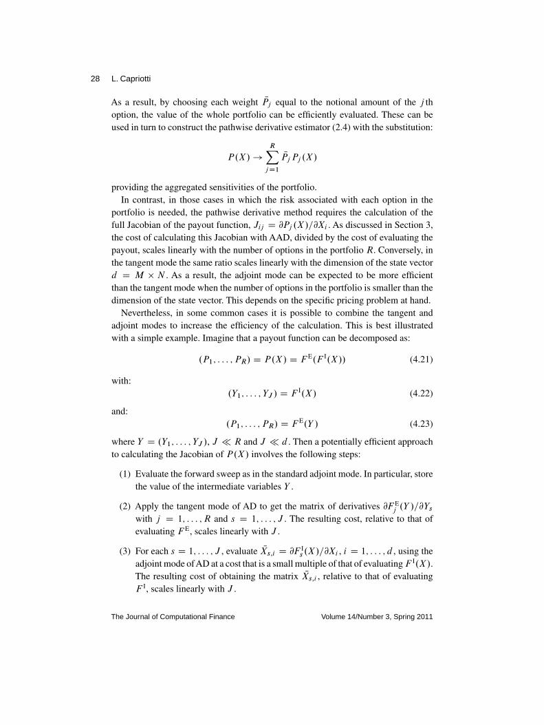
As a result, by choosing each weight NPj equal to the notional amount of the j thoption, the value of the whole portfolio can be efficiently evaluated. These can beused in turn to construct the pathwise derivative estimator (2.4) with the substitution:

P.X/!

RXjD1

NPjPj .X/

providing the aggregated sensitivities of the portfolio.In contrast, in those cases in which the risk associated with each option in the

portfolio is needed, the pathwise derivative method requires the calculation of thefull Jacobian of the payout function, Jij D @Pj .X/=@Xi . As discussed in Section 3,the cost of calculating this Jacobian with AAD, divided by the cost of evaluating thepayout, scales linearly with the number of options in the portfolio R. Conversely, inthe tangent mode the same ratio scales linearly with the dimension of the state vectord D M � N . As a result, the adjoint mode can be expected to be more efficientthan the tangent mode when the number of options in the portfolio is smaller than thedimension of the state vector. This depends on the specific pricing problem at hand.

Nevertheless, in some common cases it is possible to combine the tangent andadjoint modes to increase the efficiency of the calculation. This is best illustratedwith a simple example. Imagine that a payout function can be decomposed as:

.P1; : : : ; PR/ D P.X/ D FE.F I.X// (4.21)

with:.Y1; : : : ; YJ / D F

I.X/ (4.22)

and:.P1; : : : ; PR/ D F

E.Y / (4.23)

where Y D .Y1; : : : ; YJ /, J � R and J � d . Then a potentially efficient approachto calculating the Jacobian of P.X/ involves the following steps:

(1) Evaluate the forward sweep as in the standard adjoint mode. In particular, storethe value of the intermediate variables Y .

(2) Apply the tangent mode of AD to get the matrix of derivatives @F Ej .Y /=@Ys

with j D 1; : : : ; R and s D 1; : : : ; J . The resulting cost, relative to that ofevaluating F E, scales linearly with J .

(3) For each s D 1; : : : ; J , evaluate NXs;i D @F Is .X/=@Xi , i D 1; : : : ; d , using the

adjoint mode ofAD at a cost that is a small multiple of that of evaluatingF I.X/.The resulting cost of obtaining the matrix NXs;i , relative to that of evaluatingF I, scales linearly with J .



(4) Construct the Jacobian:

@Pj

@XiD

JXsD1

@F Ej .Y /

@YsNXs;i (4.24)

It is easy to realize that the cost of the Jacobian Ji;j divided by that of evaluatingthe payout P scales linearly with J instead of R or d . This can result in significantsavings with respect to the standard tangent or adjoint modes.

An elementary illustration of this situation is the generalization of the payouts con-sidered in the previous sections for different values of the strike price, sayK1; : : : ; KR.In these cases, the payout functions can be decomposed as:

Pj .Y / D .Y �Kj /C (4.25)

where Y is a scalar given byPNiD1wiXi .T / for the basket option, and byA.TM / for

the “best of” Asian contract. As a result, the Jacobian of the payout function reads:

@Pj .Y /

@Y

@Y

@Xi(4.26)

for i D 1; : : : ; d (d D N and d D N � M for the basket and “best of” Asianoptions, respectively) and j D 1; : : : ; R. The gradient @Pj .Y /=@Y can be evaluatedin general with the tangent mode at a cost that is a small multiple of the cost ofevaluating Equation (4.25) above. In this simple example this gives:

@Pj .Y /

@YD #.Y �Kj / (4.27)

On the other hand, the quantities @Y =@Xi are common to all the components ofthe payout function and need to be evaluated only once for all the options in theportfolio. In addition, since Y is a scalar, this can be done efficiently with theadjoint mode following exactly the same steps illustrated in Figure 4 on page 20and Figure 8 on page 25. The resulting computational cost of the Jacobian Jij D@Pj .X/=@Xi is a small multiple of the cost of evaluating the payout itself. Remark-ably, this multiple is independent of both the number of options in the portfolio andthe dimension of the state vector.

4.3 Discontinuous payouts

As recalled in Section 2, the pathwise derivative method can be applied under aspecific regularity condition requiring the payout function to be Lipschitz continu-ous (Glasserman (2004)). This requirement is generally cited in the literature as ashortcoming of the pathwise derivative method. Indeed, it potentially limits the prac-tical utility of the method to a great extent as the majority of the payout functions


30 L. Capriotti

commonly used for structured derivatives contains discontinuities, eg, in the form ofdigital features, random variables counting discrete events, or barriers.

Fortunately, the Lipschitz requirement turns out to be more of a theoretical than apractical limitation. Indeed, a practical way of addressing non-Lipschitz payouts is tosmooth out the singularities they contain. Clearly this comes at the cost of introducinga finite bias in the sensitivity estimates. However, such bias can generally be reduced tolevels that are considered more than acceptable in financial practice (see also Capriottiand Giles (2011)).

5 PATHWISE DERIVATIVE METHOD WITH ADJOINT PAYOUTS

As illustrated in the previous sections, AD, especially in the adjoint mode, allows anefficient calculation of the derivatives of the payout function, thus solving the mainimplementation difficulty of the pathwise derivative method.

Additional speed-ups can also be obtained through an efficient calculation of the tan-gent state vector. A remarkable example has been discussed, for instance, in Giles andGlasserman (2006) for the case of European options in a diffusive setting. Althoughthis approach can in principle be generalized to path-dependent options, this mayresult in a degradation of its performance, with a computational cost roughly scalingwith the number of observation times. Nonetheless, Equation (2.4) can be interpretedas a linear combination of the columns of the Jacobian defined by the tangent statevector Equation (2.5), with weights given by the derivatives of the payout function.As a result, it can be shown that the AAD paradigm can be used in general to obtain ahighly efficient implementation of the complete pathwise derivative estimator. Moreprecisely, AAD ensures that any number of sensitivities can be evaluated at a totalcomputational cost that is bounded by roughly !A ' 4 times the cost of evaluatingthe option value, independent of the number of sensitivities. A complete discussionof the implementation details of the full AAD approach is given in a forthcomingcompanion paper (Capriotti and Giles (2011)).

In the following, we will concentrate on those common cases in which the calcu-lation of the tangent state vector, and of the sum in Equation (2.4), can be efficientlyimplemented without making use of the full AAD approach (Capriotti and Giles(2010) and Capriotti and Giles (2011)). This is, for instance, the case when eachmodel parameter �k affects only a limited number of components d� � d of thestate vector. In these cases, the matrix representing the tangent state vector (2.5) canbe put in (at least approximately) block diagonal form so that both the calculationof its nonzero entries, and of the sum in Equation (2.4), can be performed at a costO.d�N� /, ie, a factor d�=d � 1 smaller than in the general case.

In a diffusive setting the situation described above is realized when each under-lying asset depends only on a limited subset of model parameters � . In these cases,



eg, commonly arising in equity or foreign exchange models, in order to calculate thetangent state vector (2.5) only one or a limited number of diffusive equations needsto be simulated for each sensitivity. In this case, it is easy to see that the computa-tional cost of the pathwise derivative method with adjoint payouts is likely to becomesmaller than that associated with bumping as the number of assets increases.

5.1 Numerical examples

5.1.1 Basket options

As a first illustration, we discuss the call option on a basket ofN assets (4.1) consideredin Section 4.1.1. Here we restrict ourselves to a lognormal model of the form:

Xi .t/ D X0i exp..r � �2i =2/t C �iWi .t// (5.1)

where X0i and �i are the spot price and volatility of the i th asset, respectively, andWi .t/ are standard Brownian motions such that EŒdWi .t/ dWj .t 0/� D �ij dt , where� is a positive semidefiniteN �N correlation matrix. In this case, it is easy to deriveanalytically the form of the tangent state vector (2.7) at any time t , eg, for delta andvega:

�i .t/ �@Xi .t/

@X0iDXi .t/

X0i(5.2)

Vi .t/ �@Xi .t/

@�iD Xi .t/.��i t CWi .t// (5.3)

respectively.This example clearly falls under the situation discussed in the introduction to this

section as each model parameter, eg, spot price or volatility, affects only a singleunderlying asset. As a result, the cost of the calculation of sensitivities by means ofthe pathwise derivative method with adjoint payouts is O.N �M/ as it is the costof calculating the value of the option, Equation (2.2). This means that all deltas andvegas for the basket call option (4.1) can be expected to be calculated at a cost that isa small multiple of the cost of calculating the value of the option, irrespective of thenumber of underlying assets in the basket.

This remarkable result is illustrated in the part (b) of Figure 9 on the next page,where we plot the processing time necessary to calculate the full delta and vega riskof the basket call option (4.1) divided by the time to calculate the value of the option,say:

RCPU DCostŒValueCRisk�

CostŒValue�(5.4)

as a function of the number of underlying assets. As expected, the cost of evaluatingthe Greeks by means of the pathwise derivative method with adjoint payouts is a small


32 L. Capriotti

FIGURE 9 Processing time ratios (5.4) for the calculation of delta and vega risk by meansof the pathwise derivative method with adjoint payouts (circles) as a function of the numberof underlying assets.

00

5 10

10

RC

PU

RC

PU

15 20

0 5 10 15 20

N

~2.8

~2.3

20

30

0

10

20

30

(b)

(a)

(a) “Best of” Asian option Equation (4.12) forM D 12 observation times. (b) Basket option.The estimated processingtime ratios for the calculation of the same sensitivities by means of bumping are also shown (triangles) for comparisonpruposes. The lines are guides for the eye.



multiple of the cost of evaluating the value of the option itself. In this case the extraoverhead is approximately 130% of the cost of calculating the option value. In contrast,the cost of estimating the same sensitivities by means of bumping grows linearly withthe number of assets. As a result, the pathwise derivative method with adjoint payoutsis computationally more efficient than bumping for any number of underlying assets,with savings larger than one order of magnitude already for medium-sized (N � 10)baskets.

5.1.2 “Best of” Asian options

As a second example, we consider the “best of” Asian option (4.12) discussed in Sec-tion 4.1.2. Here, we will report results for local volatility (Hull (2002)) diffusions sim-ulated by means of a standard Euler discretization. In particular, the drift and volatilityfunctions are assumed to take the form �i D r.t/Xi .t/ and �i D �Fi .Xi ; t /Xi .t/,where r.t/ is the deterministic instantaneous short rate, and �Fi .x; t/ is the instant-aneous volatility function for the i th asset at time t . For the sake of this discussion,as is often the case in practice, we will regard the instantaneous volatility functionas depending parametrically on the level of the “at-the-money” volatility �ATM

i .t/,namely �Fi .x; t/ D �

Fi .x; �

ATMi .t//. In the discussion below we will consider stan-

dard delta and vega with respect to a single perturbation of the at-the-money volatili-ties, namely �ATM

i .t/! �ATMi .t/C ı�ATM

i .t/. Note that this example, although morecomplex than the previous one, still falls in the category of problems in which thecalculation of each sensitivity involves the perturbation of the trajectories of just asingle underlying asset.

In part (a) of Figure 9 on the facing page we plot the processing time ratio (5.4)for the calculation of delta and vega forM D 12 observation times, and for differentnumbersN of underlying assets. As observed before for the basket option, the relativecost associated with the pathwise derivative method with adjoint payouts is indepen-dent of the number of assets. Remarkably, even for this more complicated example theextra overhead associated with the calculation of the risk is limited to approximately180% of the cost of calculating the option value. As a result, even for a single assetN D 1, the pathwise derivative method with adjoint payouts is computationally moreefficient than bumping with savings that grow linearly to over one order of magnitudealready for a relatively small number (N � 12) of underlying assets.

6 CONCLUSIONS

In this paper we have shown how algorithmic differentiation can be used to produceefficient coding for the calculation of the derivatives of the payout function, thus deal-ing with one of the main performance bottlenecks of the pathwise derivative method.With a variety of examples we demonstrated that the pathwise derivative method


34 L. Capriotti

combined with algorithmic differentiation – especially in the adjoint mode – mayprovide speed-ups of several orders of magnitude with respect to standard methods.We also showed how the tangent mode can be combined with the adjoint mode forextra performance for vectorized payouts.

In addition to Monte Carlo methods, the efficient calculation of the derivatives of thepayout function by means of algorithmic differentiation also has a natural applicationin the implementation of adjoint techniques in partial differential equation applications(Prideaux (2009)).

In forthcoming companion papers (Capriotti and Giles (2010) and Capriotti andGiles (2011)) we will build on these ideas to illustrate how AAD can be used fora highly efficient implementation of the complete pathwise derivative estimator. Inparticular, we will show how adjoint implementations like those of Giles and Glasser-man (2006) and Leclerc et al (2009) can be seen as instances of AAD. This allowsthe fast calculation of the Greeks of complex path-dependent structured derivativeswith virtually any model used in computational finance. In particular, we will discussa variety of examples, including commodity structured products, correlation modelsfor credit derivatives, the application to Bermudan options, and second-order risk.These results will demonstrate how algorithmic differentiation provides an extremelygeneral framework for the calculation of risk in financial engineering.

REFERENCES

Broadie, M., and Glasserman, P. (1996). Estimating security price derivatives using simu-lation. Management Science 42, 269–285.

Capriotti, L., and Giles, M. (2010). Fast correlation Greeks by adjoint algorithmic differen-tiation. Risk 29, 77–83.

Capriotti, L., and Giles, M. (2011). Algorithmic differentiation: adjoint Greeks made easy.In preparation.

Chen, J., and Fu, M. C. (2001). Efficient sensitivity analysis of mortgage backed securities.12th Annual Derivatives Securities Conference, unpublished.

Giles, M. (2007). Monte Carlo evaluation of sensitivities in computational finance. Proceed-ings of HERCMA Conference, Macedonia, September.

Giles, M., and Glasserman, P. (2006). Smoking adjoints: fast Monte Carlo Greeks. Risk 19,88–92.

Glasserman, P. (2004). Monte Carlo Methods in Financial Engineering. Springer.Glasserman, P., and Zhao, X. (1999). Fast Greeks by simulation in forward LIBOR models.

The Journal of Computational Finance 3, 5–39.Griewank, A. (2000). Evaluating Derivatives: Principles and Techniques of Algorithmic Dif-

ferentiation. Society for Industrial and Applied Mathematics, Philadelphia, PA.Harrison, J., and Kreps, D. (1979). Martingales and arbitrage in multiperiod securities mar-

kets. Journal of Economic Theory 20, 381–408.Hull, J. C. (2002). Options, Futures and Other Derivatives. Prentice Hall, Upper Saddle

River, NJ.



Kallenberg, O. (1997). Foundations of Modern Probability. Springer.Kunita, H. (1990). Stochastic Flows and Stochastic Differential Equations. Cambridge Uni-

versity Press.Leclerc, M., Liang, Q., and Schneider, I. (2009). Fast Monte Carlo Bermudan Greeks. Risk

22, 84–88.Prideaux, A. (2009). PhD Thesis, Oxford University.Protter, P. (1997). Stochastic Integration and Differential Equations. Springer.


Documents

Fast Greeks by algorithmic differentiation - Luca … · Fast Greeks by algorithmic differentiation 5 (or backward) mode is most efﬁcient in the more common situations where the