Fast-forwarding quantum evolutionShouzhen Gu1, Rolando D. Somma2, and Burak Şahinoğlu2

1Institute for Quantum Information and Matter, California Institute of Technology, Pasadena, CA 91125, USA2Theoretical Division, Los Alamos National Laboratory, Los Alamos, NM 87545, USA

We investigate the problem of fast-forwarding quantum evolution, whereby thedynamics of certain quantum systems can be simulated with gate complexity thatis sublinear in the evolution time. We provide a definition of fast-forwarding thatconsiders the model of quantum computation, the Hamiltonians that induce theevolution, and the properties of the initial states. Our definition accounts for anyasymptotic complexity improvement of the general case and we use it to demonstratefast-forwarding in several quantum systems. In particular, we show that some localspin systems whose Hamiltonians can be taken into block diagonal form using an effi-cient quantum circuit, such as those that are permutation-invariant, can be exponen-tially fast-forwarded. We also show that certain classes of positive semidefinite localspin systems, also known as frustration-free, can be polynomially fast-forwarded, pro-vided the initial state is supported on a subspace of sufficiently low energies. Last, weshow that all quadratic fermionic systems and number-conserving quadratic bosonicsystems can be exponentially fast-forwarded in a model where quantum gates are ex-ponentials of specific fermionic or bosonic operators, respectively. Our results extendthe classes of physical Hamiltonians that were previously known to be fast-forwarded,while not necessarily requiring methods that diagonalize the Hamiltonians efficiently.We further develop a connection between fast-forwarding and precise energy mea-surements that also accounts for polynomial improvements.

Accepted in Quantum 2021-10-29, click title to verify. Published under CC-BY 4.0. 1

arX

iv:2

105.

0730

4v2

[qu

ant-

ph]

6 N

ov 2

021

Contents1 Introduction 2

2 Concepts and definitions 4

3 Fast-forwarding of local spin systems 73.1 Block diagonalization . . . . . . . . . . . . . . . . . . . . . . . . . . . . . . . . . . 8

3.1.1 Permutation-invariant spin Hamiltonians . . . . . . . . . . . . . . . . . . . 93.2 Frustration-free spin Hamiltonians at low-energies . . . . . . . . . . . . . . . . . . 13

4 Fast-forwarding of fermionic and bosonic systems 164.1 Lie-algebra diagonalization . . . . . . . . . . . . . . . . . . . . . . . . . . . . . . . 17

4.1.1 Quadratic fermionic Hamiltonians . . . . . . . . . . . . . . . . . . . . . . 204.1.2 Quadratic bosonic Hamiltonians . . . . . . . . . . . . . . . . . . . . . . . 20

5 Fast-forwarding and energy measurements 21

6 Conclusions and outlook 23

7 Acknowledgements 23

A Complexity of block diagonalizing permutation-invariant qubit Hamiltonians 27

B Proof of Theorem 5.3 28

1 IntroductionSince Feynman’s initial proposal of simulating physics with quantum computers [1], a significantamount of research in quantum computing has focused on quantum algorithms for Hamiltoniansimulation, i.e., the problem of simulating the time evolution of a quantum system inducedby a Hamiltonian H. The main figure of efficiency is how the quantum complexity of thesealgorithms, as determined by the number of elementary (e.g., two-qubit) gates, scales withvarious parameters such as the evolution time t > 0. To date, the most efficient known methodsfor Hamiltonian simulation have quantum complexities that are almost linear in t (cf., [2–14]).These methods are thus optimal since simulating all quantum systems with complexity sublinearin t is impossible [4, 15, 16].

Nevertheless, a natural question is whether such complexities can be significantly reduced inspecific cases, opening up the possibility of fast-forwarding Hamiltonian simulation. Roughly, aquantum system or Hamiltonian is said to be fast-forwarded if its time evolution can be simulatedwith quantum complexity scaling sublinearly in t. An answer to this question is relevant for bothfoundational and practical reasons. For example, the ability to fast-forward a Hamiltonian mightallow us to study physical systems on quantum computers more rapidly. It could also result inother important quantum speedups, as some well-known quantum algorithms use Hamiltoniansimulation as a subroutine (cf., [17, 18]).

Indeed, a few examples of exponential fast-forwarding are known [15], in which there existquantum algorithms for Hamiltonian simulation of quantum complexity at most polylogarithmicin t. These examples include Hamiltonians that can be diagonalized via an efficient quantumcircuit, commuting local Hamiltonians, and quadratic fermionic Hamiltonians [19–21]. Butwhile these cases are interesting and demonstrate the possibility of fast-forwarding, they are

2

only a handful, and the field of fast-forwarding quantum evolution remains largely unexplored.Characterizing larger classes of Hamiltonians that can be fast-forwarded is crucial.

In this paper, we further explore the theme of fast-forwarding and present new examples thatcan be fast-forwarded. To this end, we first provide a definition of fast-forwarding that accountsfor any asymptotic complexity improvement of the general case, going beyond the exponentialfast-forwarding studied previously [15]. We also consider the problem of fast-forwarding insubspaces, which concerns the case where quantum evolution occurs only in a certain subspaceof the full Hilbert space. This notion of subspace fast-forwarding is useful for simulating physicalsystems because often the evolution occurs in certain subspaces of, for example, low energies orcertain preserved symmetries [22–24]. Moreover, since certain quantum systems (e.g., bosonicsystems) cannot be directly simulated on a digital quantum computer, we provide a definition offast-forwarding that is relative to a specified set of observables. The “elementary gates” in thiscase correspond to certain unitary operators that are exponentials of these observables. Thesedefinitions are presented in detail in Sec. 2.

Following these definitions, we present several examples of quantum systems that can befast-forwarded and provide detailed constructions for simulating their time evolution. Theseare:

Block diagonalizable Hamiltonians: A class of Hamiltonians that can be exponentiallyfast-forwarded consists of those Hamiltonians that can be brought into block diagonal form withan efficient quantum circuit if each block can be computed efficiently and fast-forwarded. Weinvestigate fast-forwarding based on this property in Sec. 3.1 for spin systems. A particularcase, which is analyzed in Sec. 3.1.1, is the class of spin Hamiltonians that are invariant underpermutations of spins (and thus preserve the magnitude of the total angular momentum). In thiscase, we achieve exponential fast-forwarding by employing the Schur transform [25, 26], whichblock diagonalizes the Hamiltonian in the angular momentum subspaces.

Frustation-free Hamiltonians at low energies: In Sec. 3.2, we investigate subspace fast-forwarding for certain positive Hamiltonians of spin systems, which include those that satisfy afrustration-free property [27, 28]. We show that these Hamiltonians can be polynomially fast-forwarded when the input states are guaranteed to be in a certain low-energy subspace. Weachieve fast-forwarding by using the spectral gap amplification method given in Refs. [29, 30] incombination with quantum phase estimation [31, 32].

Fermionic and bosonic Hamiltonians: In Sec. 4, we study exponential fast-forwardingin quadratic fermionic and bosonic Hamiltonians. We first consider a Lie algebraic setting andfocus on Lie algebraic models of quantum computation, where the quantum gates correspond tocertain unitary transformations induced by the algebra. In Sec. 4.1 we describe exponential fast-forwarding via Lie-algebra diagonalization. We then apply the technique to formalize a resulton exponential fast-forwarding of quadratic fermionic Hamiltonians (Sec. 4.1.1) and number-conserving quadratic bosonic Hamiltonians (Sec. 4.1.2).

Our results address the simulation of quantum systems that are abundant in physics. Thesesystems include condensed matter spin models and quantum chemistry and nuclear physicsmodels, such as the well-known Lipkin-Meshkov-Glick model [33], which preserve the magnitudeof the total angular momentum. Frustration-free Hamiltonians are also ubiquitous and includethe AKLT model [34] and, more generally, those “parent” Hamiltonians that appear in thecontext of projected entangled pair states (PEPS) [27]. While a complexity improvement forsimulating these systems under the assumption that the initial state is supported in a low-energysubspace was shown in Ref. [22], that result does not demonstrate fast-forwarding as the quantumcomplexity is still superlinear in t. Fermionic and bosonic Hamiltonians are also important, andfast simulation methods for these systems will play an important role in the general problem of

3

simulating quantum field theories [35]. Our methods exploit different properties of these systemsand go beyond the fast-forwarding approach based on diagonalization.

Last, we note that our definitions immediately lead us to a generalization of the correspon-dence between fast-forwarding and precise energy measurements discussed in Ref. [15]. In Sec. 5we show that, roughly, polynomial fast-forwarding is equivalent to polynomially-precise energymeasurements in qubit systems.

2 Concepts and definitionsFor a given Hamiltonian H and t > 0, Hamiltonian simulation methods aim at simulatingthe evolution operator U(t) := e−itH . They do this by implementing a sequence of “elementary”quantum gates, and the number of these gates determines the quantum complexity of the method.This complexity depends on parameters such as t, system size, and precision. The fast-forwardingproblem is then focused on finding fast ways of simulating U(t), where the figure of merit is thequantum complexity and its asymptotic scaling, particularly with t. Roughly, a Hamiltonian issaid to be fast-forwarded if this complexity is sublinear in t.

Several points must be addressed before providing precise definitions of fast-forwarding. First,the quantum complexity depends on the computational model under consideration, which speci-fies what the elementary quantum gates are. Usually, these quantum gates are chosen to be com-patible with physical implementations. For example, in the standard circuit model of quantumcomputation, elementary quantum gates may correspond to two-qubit gates. For a fermionic orbosonic model of computation, elementary gates correspond to simple unitary operators inducedby corresponding fermionic or bosonic algebras.

Definition 2.1 (Models of quantum computation). A model of quantum computation can bespecified by a set of observables h = O1, O2, . . . acting on a Hilbert space H. The elementaryquantum gates are unitary transformations expressed as exponentials e−iθlOl, where θl ∈ R and|θl| ≤ 1. A quantum circuit in this model is a sequence of elementary quantum gates, and thenumber of these gates is the quantum complexity.

The condition |θl| ≤ 1 is arbitrary – i.e., we can bound the phases by a different constant– but is needed to restrict the power of each quantum gate. This is particularly relevant inbosonic models of computation where, in contrast with certain two-qubit gates (induced byPauli operators), bosonic gates are not periodic in θl.

Second, known no-fast-forwarding results [4, 15, 16] place a lower bound on the worst-casequantum complexity for simulating classes of Hamiltonians as long as the evolution time satisfiest ≤ T , where T depends on certain problem parameters, such as the number of qubits or spins.These lower bounds are commonly presented as asymptotic scalings. If the Hamiltonian is fixed,however, it may be possible to simulate that particular Hamiltonian with quantum complexitythat has a very mild (polylogarithmic) dependence on t, for example, by exact diagonalizationfor large t. Since the asymptotic scaling of the quantum complexity with t and other parametersis in general of relevance, we will consider sequences of Hamiltonians Hnn that depend ona “system-size” parameter n = 1, 2, . . .. For qubit systems, n is the number of qubits. Forfermionic or bosonic systems, n can be the number of modes. By allowing the system size togrow, we are able to consider maximum evolution times that increase in order to determine thetrue asymptotic scaling of the gate complexity. For the problem of fast-forwarding quantumevolution, it is then important to determine the parameters of Hamiltonian simulation preciselyas a function of n, which are defined as follows:

4

Definition 2.2 (Hamiltonian-simulation parameters). Let Hnn be a sequence of Hamiltoniansacting on Hilbert spaces Hnn. The quantum circuits Vn(t)n,t simulate the HamiltoniansHnn on subspaces Sn ⊆ Hnn with parameters (T (n), ε(n), G(n)) if the quantum complexityis at most G(n) in a given model of quantum computation and, for each n, all |ψn〉 ∈ Sn, andall t ≤ T (n), ∥∥∥(e−itHn ⊗ 1lA − Vn(t)) |ψn〉 ⊗ |0〉A

∥∥∥ ≤ ε(n) . (1)

The operator 1lA is the identity operator acting on an ancillary register A and |0〉A is somesimple initial state for that register.

Throughout this paper, ‖ |φ〉 ‖ is the Euclidean norm of the quantum state |φ〉 and ‖A‖ isthe spectral norm of the operator A.

Definition 2.2 concerns the largest quantum complexity, G(n), for approximating e−itHn forall times t ≤ T (n). While this is not necessary, we will see that understanding the asymptoticbehavior of G(n) alone will suffice to classify many classes of Hamiltonians that can be fast-forwarded, including previously known examples and the examples we provide in the followingsections. Nevertheless, one may be interested in the ability of fast-forwarding in, for example,other specific regions of t, in which case the above definition could be adapted to that setting.

It is important to remark that a circuit Vn(t) might include operations during a pre- orpost-processing step. In some cases these steps can be implemented on a classical computer(see the examples in Sec. 4), but we will assume they are all part of the quantum operationthat simulates the Hamiltonian, thereby avoiding any complication in separating quantum andclassical complexities. Some examples in this paper do require some form of pre-processing, butthe complexity of such a step is not dominant in those cases.

Last, any useful definition of fast-forwarding must capture the ability to simulate a partic-ular Hamiltonian (or a class of Hamiltonians) with quantum complexity that is below a lowerbound established for worst-case instances of a class. For example, one can establish a no-fast-forwarding theorem for the class of local spin Hamiltonians [16] that would apply to the worstcase, but there are still local Hamiltonians in that class that can be simulated more rapidly withquantum complexity that is sublinear in t, such as XY Ising models [19]. The no-fast-forwardingline, which we define below, will play an important role in a definition of fast-forwarding.

Definition 2.3 (No-fast-forwarding line). Let Cnn denote classes of Hamiltonians, i.e. Cn isa subset of the Hermitian operators acting on Hn, and let T (n) ≥ 0 and ε(n) ≥ 0 be functions ofn. The no-fast-forwarding line l(n) with respect to these classes is the function

l(n) = maxHn∈Cn

minVn(t)t

G(n) , (2)

where the quantum circuits Vn(t)t simulate the Hamiltonian Hn ∈ Cn with parameters(T (n), ε(n), G(n)).

That is, for a given n, the no-fast-forwarding line is the minimum quantum complexityrequired for simulating every Hamiltonian in a given class and quantum computational model.This line depends on the maximum simulation time T (n); however, in our analyses and examplesT (n) is a fixed function of n and we do not need to consider this dependence explicitly.

If a particular sequence of Hamiltonians of those classes can be simulated with less quantumcomplexity, i.e. asymptotically less than l(n), then we will claim that such a Hamiltoniansequence can be fast-forwarded. In more detail, we define fast-forwarding as follows:

5

Definition 2.4 (Fast-forwarding). Let Cnn denote classes of Hamiltonians, i.e. Cn is a subsetof the Hermitian operators acting on Hn, and let T (n) ≥ 0 and ε(n) ≥ 0 be functions of n.The quantum circuits Vn(t)n,t are said to be (T (n), ε(n), G(n))-fast-forwarding a Hamiltoniansequence Hn ∈ Cnn on subspaces Snn if the following hold:

1. The quantum circuits Vn(t)n,t simulate the Hamiltonians Hnn with parameters(T (n), ε(n), G(n)), and

2.

limn→∞

G(n)l(n) = 0 . (3)

Our definition of fast-forwarding is relative to the classes of Hamiltonians Cnn, and thisis needed because certain classes are more difficult to simulate than others. If, however, thoseclasses are chosen to be too restrictive, then the definition will not capture the ability to fast-forward a Hamiltonian in an interesting class. For example, a diagonal qubit Hamiltonian Hn

may not be fast-forwarded relative to a class Cnn of diagonal qubit Hamiltonians despite hav-ing an algorithm of polylogarithmic complexity in t because every Hamiltonian in Cn can besimulated with such complexity. But if Cnn are more general, not necessarily diagonal qubitHamiltonians, and Hn ∈ Cn is diagonal, then the definition will serve its purpose. Likewise, wewill require Cnn and Hnn to consist of Hamiltonians that are normalized in some way. Oth-erwise, l(n) and G(n) could be artificially large or small, respectively, implying fast-forwardingunder our definition.

Definition 2.4 also depends on a Hamiltonian sequence Hnn with no explicit requirementthat these Hamiltonians are related in some way. Nevertheless, the definition becomes usefulwhen the sequence describes the “same” type of Hamiltonians for different system sizes n. Forexample, Hn may be constructed from Hn−1 by adding a term that involves a new subsystem;e.g., the n-th spin or the n-th fermionic or bosonic mode. We sometimes refer to such sequencesas meaningful sequences of Hamiltonians and define them more precisely for spin and fermionicor bosonic systems in Secs. 3 and 4, respectively. Similarly, while no requirement is set for thesubspaces Snn, the definition will be useful when Sn is related to Sn−1 in some way (e.g.,Sn ≡ Hn). For simplicity, we will be concerned with the simulation of Hamiltonians to constanterror ε(n) = ε, but our results can be easily generalized to other cases.

It is generally difficult to find the no-fast-forwarding line l(n). To show that a Hamiltoniancan be fast-forwarded, we often show that it can be simulated with asymptotic quantum com-plexity that grows slower in t than a lower bound l′(n, t) of l(n). These lower bounds, also knownas no-fast-forwarding theorems, are known for some classes of Hamiltonians. Reference [16], forexample, provides this lower bound for the class of geometrically-local qubit Hamiltonians, al-though these Hamiltonians are time-dependent. In this case, l′(n, t) = Ω(nt) for t ≤ T (n) = 4nand thus l(n) = Ω(n4n). Related is a result of Ref. [15] that strongly suggests that no exponen-tial fast-forwarding is possible for all n-qubit Hamiltonians that are 2-sparse, where the matrixof Hn has at most two nonzero elements per row/column. Other known lower bounds apply tothe setting in which Hamiltonians can be accessed via a black-box unitary [4]. These resultssuggest that for some classes of Hamiltonians analyzed in this paper, the no-fast-forwarding linesatisfies l(n) = Ω(nT (n)), where T (n) is exponential in n (e.g., T (n) = 4n). When the no-fast-forwarding line has this form, Def. 2.4 coincides with the intuitive notion of fast-forwarding asa simulation algorithm achieving complexity scaling sublinearly in the evolution time.

The various types of fast-forwarding can be characterized by the asymptotic behavior ofG(n) and l(n). For example, for the exponential fast-forwarding problem analyzed in Ref. [15],

6

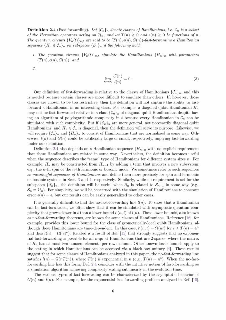
a class of Hamiltonians can be simulated with quantum complexity G(n) = O(poly(n)) while l(n)(or T (n)) is exponential in n. Our definition, however, allows for more general cases, includingpolynomial fast-forwarding. This occurs when, in particular, both G(n) and l(n) are exponentialin n, but G(n)/l(n)→ 0. For example, a Hamiltonian simulation method of quantum complexitythat scales as ntα for α < 1 and all t ≤ T (n) = 4n, will imply polynomial fast-forwarding relativeto a class of Hamiltonians with no-fast-forwarding line of the form l(n) = Ω(n4n). In Fig. 1 wesketch examples of fast-forwarding and no-fast-forwarding using our definitions, where all therelevant quantities are increasing in n or t.

<latexit sha1_base64="l/Odks7TyaE4AV3B3z48tDptAxQ=">AAAB7nicbVBNS8NAEJ3Ur1q/qh69LBbBiyURUY9FLz1WsB/QhrLZbtqlm03YnQgl9Ed48aCIV3+PN/+N2zYHbX0w8Hhvhpl5QSKFQdf9dgpr6xubW8Xt0s7u3v5B+fCoZeJUM95ksYx1J6CGS6F4EwVK3kk0p1EgeTsY38/89hPXRsTqEScJ9yM6VCIUjKKV2vV+pi68ab9ccavuHGSVeDmpQI5Gv/zVG8QsjbhCJqkxXc9N0M+oRsEkn5Z6qeEJZWM65F1LFY248bP5uVNyZpUBCWNtSyGZq78nMhoZM4kC2xlRHJllbyb+53VTDG/9TKgkRa7YYlGYSoIxmf1OBkJzhnJiCWVa2FsJG1FNGdqESjYEb/nlVdK6rHrXVffhqlK7y+Mowgmcwjl4cAM1qEMDmsBgDM/wCm9O4rw4787HorXg5DPH8AfO5w/BKY8w</latexit>

Hn1

<latexit sha1_base64="+a9cKOls/fqCYj95ABImtSRj2uc=">AAAB7HicbVBNS8NAEJ3Ur1q/qh69LBbBU0lE1GPRS48VTFtoQ9lsN+3SzSbsToQS+hu8eFDEqz/Im//GbZuDVh8MPN6bYWZemEph0HW/nNLa+sbmVnm7srO7t39QPTxqmyTTjPsskYnuhtRwKRT3UaDk3VRzGoeSd8LJ3dzvPHJtRKIecJryIKYjJSLBKFrJbw5yNRtUa27dXYD8JV5BalCgNah+9ocJy2KukElqTM9zUwxyqlEwyWeVfmZ4StmEjnjPUkVjboJ8ceyMnFllSKJE21JIFurPiZzGxkzj0HbGFMdm1ZuL/3m9DKObIBcqzZArtlwUZZJgQuafk6HQnKGcWkKZFvZWwsZUU4Y2n4oNwVt9+S9pX9S9q7p7f1lr3BZxlOEETuEcPLiGBjShBT4wEPAEL/DqKOfZeXPel60lp5g5hl9wPr4B5R2Ovg==</latexit>

Hn

Quantum complexity

<latexit sha1_base64="Pr5aPgXpcw4NaU2PSo9hhymmHUg=">AAAB6HicbVBNS8NAEN3Ur1q/qh69LBbBU0lE1GPRi8cW7Ae0oWy2k3btZhN2J0IJ/QVePCji1Z/kzX/jts1BWx8MPN6bYWZekEhh0HW/ncLa+sbmVnG7tLO7t39QPjxqmTjVHJo8lrHuBMyAFAqaKFBCJ9HAokBCOxjfzfz2E2gjYvWAkwT8iA2VCAVnaKUG9ssVt+rOQVeJl5MKyVHvl796g5inESjkkhnT9dwE/YxpFFzCtNRLDSSMj9kQupYqFoHxs/mhU3pmlQENY21LIZ2rvycyFhkziQLbGTEcmWVvJv7ndVMMb/xMqCRFUHyxKEwlxZjOvqYDoYGjnFjCuBb2VspHTDOONpuSDcFbfnmVtC6q3lXVbVxWard5HEVyQk7JOfHINamRe1InTcIJkGfySt6cR+fFeXc+Fq0FJ585Jn/gfP4A4c+M/Q==</latexit>

t<latexit sha1_base64="7T3WM1WP3X3S3GW2BdM40W/7Zn0=">AAAB7XicbVBNSwMxEJ2tX7V+VT16CRahHiy7RdRj0YvHCv2CdinZNNvGZpMlyQpl6X/w4kERr/4fb/4b03YP2vpg4PHeDDPzgpgzbVz328mtrW9sbuW3Czu7e/sHxcOjlpaJIrRJJJeqE2BNORO0aZjhtBMriqOA03Ywvpv57SeqNJOiYSYx9SM8FCxkBBsrtRplceGd94slt+LOgVaJl5ESZKj3i1+9gSRJRIUhHGvd9dzY+ClWhhFOp4VeommMyRgPaddSgSOq/XR+7RSdWWWAQqlsCYPm6u+JFEdaT6LAdkbYjPSyNxP/87qJCW/8lIk4MVSQxaIw4chINHsdDZiixPCJJZgoZm9FZIQVJsYGVLAheMsvr5JWteJdVdyHy1LtNosjDydwCmXw4BpqcA91aAKBR3iGV3hzpPPivDsfi9ack80cwx84nz8eEY4s</latexit>

T (n 1)<latexit sha1_base64="r2OfO330QalROMt/ADTjiWI/hvE=">AAAB63icbVBNSwMxEJ2tX7V+VT16CRahXsquFPVY9OKxQr+gXUo2zbahSXZJskJZ+he8eFDEq3/Im//GbLsHbX0w8Hhvhpl5QcyZNq777RQ2Nre2d4q7pb39g8Oj8vFJR0eJIrRNIh6pXoA15UzStmGG016sKBYBp91gep/53SeqNItky8xi6gs8lixkBJtMalXl5bBccWvuAmideDmpQI7msPw1GEUkEVQawrHWfc+NjZ9iZRjhdF4aJJrGmEzxmPYtlVhQ7aeLW+fowiojFEbKljRoof6eSLHQeiYC2ymwmehVLxP/8/qJCW/9lMk4MVSS5aIw4chEKHscjZiixPCZJZgoZm9FZIIVJsbGU7IheKsvr5POVc27rrmP9UrjLo+jCGdwDlXw4AYa8ABNaAOBCTzDK7w5wnlx3p2PZWvByWdO4Q+czx9DVY26</latexit>

T (n)

<latexit sha1_base64="cKaFIDTVQHg4+BkyhlhXPjQKImA=">AAAB7nicdVDLSgMxFM3UV62vqks3wSJWkCEzDm3dFd24rGAf0A4lk2ba0ExmSDJCKf0INy4Ucev3uPNvzLQVVPTAhcM593LvPUHCmdIIfVi5ldW19Y38ZmFre2d3r7h/0FJxKgltkpjHshNgRTkTtKmZ5rSTSIqjgNN2ML7O/PY9lYrF4k5PEupHeChYyAjWRmrz07I412f9YgnZl7WK61UgshGqOq6TEbfqXXjQMUqGElii0S++9wYxSSMqNOFYqa6DEu1PsdSMcDor9FJFE0zGeEi7hgocUeVP5+fO4IlRBjCMpSmh4Vz9PjHFkVKTKDCdEdYj9dvLxL+8bqrDmj9lIkk1FWSxKEw51DHMfocDJinRfGIIJpKZWyEZYYmJNgkVTAhfn8L/Scu1nYqNbr1S/WoZRx4cgWNQBg6ogjq4AQ3QBASMwQN4As9WYj1aL9brojVnLWcOwQ9Yb59oiY75</latexit>

l0(n, t)

<latexit sha1_base64="hBdq3r89g5fq4uf7BvTULKdgcJg=">AAAB8HicdVDLSsNAFJ3UV62vqks3g0WsoCGJoa27ohuXFexD2lAm00k7dDIJMxOhhH6FGxeKuPVz3Pk3TtoKKnrgwuGce7n3Hj9mVCrL+jByS8srq2v59cLG5tb2TnF3ryWjRGDSxBGLRMdHkjDKSVNRxUgnFgSFPiNtf3yV+e17IiSN+K2axMQL0ZDTgGKktHTHjsv8zD5VJ/1iyTIvahXHrUDLtKyq7dgZcaruuQttrWQogQUa/eJ7bxDhJCRcYYak7NpWrLwUCUUxI9NCL5EkRniMhqSrKUchkV46O3gKj7QygEEkdHEFZ+r3iRSFUk5CX3eGSI3kby8T//K6iQpqXkp5nCjC8XxRkDCoIph9DwdUEKzYRBOEBdW3QjxCAmGlMyroEL4+hf+TlmPaFdO6cUv1y0UceXAADkEZ2KAK6uAaNEATYBCCB/AEng1hPBovxuu8NWcsZvbBDxhvn0SLj2s=</latexit>

l0(n 1, t)

<latexit sha1_base64="/TNU7rA4ZBgofvn13nHUhNMgMqM=">AAAB63icdVDLSsNAFJ3UV62vqks3g0WomzCJoa27ohuXFewD2lAm00k7dDIJMxOhhP6CGxeKuPWH3Pk3TtoKKnrgwuGce7n3niDhTGmEPqzC2vrG5lZxu7Szu7d/UD486qg4lYS2Scxj2QuwopwJ2tZMc9pLJMVRwGk3mF7nfveeSsVicadnCfUjPBYsZATrXOJVcT4sV5B92ai5Xg0iG6G64zo5cevehQcdo+SogBVaw/L7YBSTNKJCE46V6jso0X6GpWaE03lpkCqaYDLFY9o3VOCIKj9b3DqHZ0YZwTCWpoSGC/X7RIYjpWZRYDojrCfqt5eLf3n9VIcNP2MiSTUVZLkoTDnUMcwfhyMmKdF8ZggmkplbIZlgiYk28ZRMCF+fwv9Jx7Wdmo1uvUrzahVHEZyAU1AFDqiDJrgBLdAGBEzAA3gCz1ZkPVov1uuytWCtZo7BD1hvn8gMjhQ=</latexit>

l(n)

<latexit sha1_base64="9FT97TGQjgSe8tUlBXOUOaZbUDA=">AAAB7XicdVDLSgMxFM3UV62vqks3wSLUhcPMOLR1V3TjsoJ9QDuUTJppYzPJkGSEUvoPblwo4tb/ceffmGkrqOiBC4dz7uXee8KEUaUd58PKrayurW/kNwtb2zu7e8X9g5YSqcSkiQUTshMiRRjlpKmpZqSTSILikJF2OL7K/PY9kYoKfqsnCQliNOQ0ohhpI7VYmZ+5p/1iybEvahXPr0DHdpyq67kZ8ar+uQ9do2QogSUa/eJ7byBwGhOuMUNKdV0n0cEUSU0xI7NCL1UkQXiMhqRrKEcxUcF0fu0MnhhlACMhTXEN5+r3iSmKlZrEoemMkR6p314m/uV1Ux3VginlSaoJx4tFUcqgFjB7HQ6oJFiziSEIS2puhXiEJMLaBFQwIXx9Cv8nLc92K7Zz45fql8s48uAIHIMycEEV1ME1aIAmwOAOPIAn8GwJ69F6sV4XrTlrOXMIfsB6+wSi+I6G</latexit>

l(n 1)

<latexit sha1_base64="A78D3EzSkR5O4fqePUXDVuj1TyE=">AAAB/XicbVDLSgMxFM3UV62v8bFzEyxCXbTMiKjLolBdVrAPaIchk6ZtaCYZkoxQh8FfceNCEbf+hzv/xrSdhbYeuHA4517uvSeIGFXacb6t3NLyyupafr2wsbm1vWPv7jWViCUmDSyYkO0AKcIoJw1NNSPtSBIUBoy0gtH1xG89EKmo4Pd6HBEvRANO+xQjbSTfPrjxk6QrQ8hFuVZL0xIvuye+XXQqzhRwkbgZKYIMdd/+6vYEjkPCNWZIqY7rRNpLkNQUM5IWurEiEcIjNCAdQzkKifKS6fUpPDZKD/aFNMU1nKq/JxIUKjUOA9MZIj1U895E/M/rxLp/6SWUR7EmHM8W9WMGtYCTKGCPSoI1GxuCsKTmVoiHSCKsTWAFE4I7//IiaZ5W3POKc3dWrF5lceTBITgCJeCCC1AFt6AOGgCDR/AMXsGb9WS9WO/Wx6w1Z2Uz++APrM8fvu6UHA==</latexit>

GnoFF(n 1)

<latexit sha1_base64="Pe2RYdRoPlZOFDp33vEcWv8otV0=">AAAB+3icbVDLSsNAFJ3UV62vWJduBotQF5ZERF0Wheqygn1AG8JkOmmHzkzCzEQsIb/ixoUibv0Rd/6N0zYLbT1w4XDOvdx7TxAzqrTjfFuFldW19Y3iZmlre2d3z94vt1WUSExaOGKR7AZIEUYFaWmqGenGkiAeMNIJxjdTv/NIpKKReNCTmHgcDQUNKUbaSL5dvvXTtC85FNFpo5FlVXHi2xWn5swAl4mbkwrI0fTtr/4gwgknQmOGlOq5Tqy9FElNMSNZqZ8oEiM8RkPSM1QgTpSXzm7P4LFRBjCMpCmh4Uz9PZEirtSEB6aTIz1Si95U/M/rJTq88lIq4kQTgeeLwoRBHcFpEHBAJcGaTQxBWFJzK8QjJBHWJq6SCcFdfHmZtM9q7kXNuT+v1K/zOIrgEByBKnDBJaiDO9AELYDBE3gGr+DNyqwX6936mLcWrHzmAPyB9fkD2VaTqg==</latexit>

GnoFF(n)

<latexit sha1_base64="Xv0oaVeeKGAzgSvie1aGeRmIvtw=">AAAB+HicdVDLSgMxFM3UV62Pjrp0EyxC3ZSkSB+7olBdVrAPaEvJpGkbmskMSUaoQ7/EjQtF3Pop7vwbM20FFT1w4XDOvdx7jxcKrg1CH05qbX1jcyu9ndnZ3dvPugeHLR1EirImDUSgOh7RTHDJmoYbwTqhYsT3BGt708vEb98xpXkgb80sZH2fjCUfcUqMlQZu9moQxz3lw3p9Ps/Ls4GbQwWEEMYYJgSXS8iSarVSxBWIE8siB1ZoDNz33jCgkc+koYJo3cUoNP2YKMOpYPNML9IsJHRKxqxrqSQ+0/14cfgcnlplCEeBsiUNXKjfJ2Liaz3zPdvpEzPRv71E/MvrRmZU6cdchpFhki4XjSIBTQCTFOCQK0aNmFlCqOL2VkgnRBFqbFYZG8LXp/B/0ioWcKmAbs5ztYtVHGlwDE5AHmBQBjVwDRqgCSiIwAN4As/OvfPovDivy9aUs5o5Aj/gvH0CEjySuA==</latexit>

GFF(n)<latexit sha1_base64="+7lJ+iZlcAAfM0QQ96lS/SBPl4U=">AAAB+nicdVDLSgMxFM3UV62vVpdugkWoC0tSpI9dUaguK9gHtKVk0rQNzWSGJKOUsZ/ixoUibv0Sd/6NmbaCih64cDjnXu69xw0E1wahDyexsrq2vpHcTG1t7+zupTP7Te2HirIG9YWv2i7RTHDJGoYbwdqBYsRzBWu5k4vYb90ypbkvb8w0YD2PjCQfckqMlfrpzGU/irrKg7XabJaTp/ikn86iPEIIYwxjgktFZEmlUi7gMsSxZZEFS9T76ffuwKehx6ShgmjdwSgwvYgow6lgs1Q31CwgdEJGrGOpJB7TvWh++gweW2UAh76yJQ2cq98nIuJpPfVc2+kRM9a/vVj8y+uEZljuRVwGoWGSLhYNQwGND+Mc4IArRo2YWkKo4vZWSMdEEWpsWikbwten8H/SLORxMY+uz7LV82UcSXAIjkAOYFACVXAF6qABKLgDD+AJPDv3zqPz4rwuWhPOcuYA/IDz9gn1pZMq</latexit>

GFF(n 1)

Figure 1: Examples of fast-forwarding and no-fast-forwarding according to Def. 2.4. For fast-forwarding,the quantum complexity GFF (n) crosses the lower bound l′(n, t) and lies under the no-fast-forwarding linel(n), and GFF(n)/l(n) → 0. For no-fast-forwarding, the quantum complexity Gno−FF(n) lies above l(n).Exponential or polynomial fast-forwarding is obtained depending on the asymptotic behavior of G(n) and l(n).The Hamiltonians Hnn belong to classes Cnn and model quantum systems of different sizes n.

In the following, we assume ~ = 1 and do not assign units to Hamiltonians or time, which iscommon practice for analyzing quantum simulation algorithms. Nevertheless, if one is interestedin the resulting complexity in an actual application where units are considered, this will easilyfollow from our results. We also use A, A′, etc., to denote ancillary systems, which includeall additional systems required by a particular Hamiltonian simulation approach, such as thoseneeded to implement certain classical computations reversibly.

3 Fast-forwarding of local spin systemsIn this section, we consider fast-forwarding relative to the class of local spin systems, where nspins are located at the vertices of lattices Λn, n = 1, 2, . . .. Each spin is of dimension d, and foreach n, the Hilbert space is Hn =

(Cd)⊗n

. For each system there is a Hamiltonian Hn actingon Hn that describes the interactions. This Hamiltonian is a sum of (local) Hermitian terms;that is, Hn =

∑X⊂Λn hX , where hX describes the interactions of spins in a subset X ⊂ Λn. We

detail the structure of these Hamiltonians by assuming them to be k-local and of degree g. Thismeans that each subset X involves at most k spins, and each spin is involved in at most g ofthe subsets X. For simplicity, we take k and g to be constant and also assume ‖hX‖ ≤ 1, for allX. The no-fast-forwarding line is assumed to be l(n) = Ω(nT (n)), where T (n) = d2n.

7

The meaningful Hamiltonian sequences Hnn are such that Hn = Hn−1⊗1ln+vn, where vnis a sum of interaction terms that act non-trivially on the new (n-th) spin and other spins of thesystem. The Hilbert spaces are such that Hn = Hn−1⊗Cd and 1ln is the identity operator on Cd,the space associated with the new spin. We are interested in the complexity of simulating spinHamiltonians in the standard gate-based model, where elementary quantum gates are two-qubitgates. Nevertheless, some results of this section apply to more general quantum systems thatare not necessarily spin systems.

The first example of fast-forwarding of a spin system is described in Sec. 3.1, where we studyHamiltonians with certain block diagonal structure, which occurs due to a symmetry of thesystem. Roughly, if a Hamiltonian can be taken to a block diagonal form via a unitary thatadmits an efficient quantum circuit implementation, and the block diagonal Hamiltonian can besimulated with complexity sublinear in t, then the original Hamiltonian can be fast-forwarded.This occurs, for example, when the Hamiltonian is invariant under the permutation of spins,such as for the well-known Lipkin-Meshkov-Glick model [33], and we show that this case can beexponentially fast-forwarded. Permutation-invariant spin Hamiltonians have also been used inquantum computing for noise protection [36] and optimization [37].

The second example is described in Sec. 3.2, where we study the so-called parent or frustration-free Hamiltonians in the context of subspace fast-forwarding. We show that these Hamiltonianscan be polynomially fast-forwarded if the subspaces Sn are those of “low” energies. The actuallevel of fast-forwarding depends on the parameters of the problem, especially on a low-energycutoff ∆, which might depend on the evolution time t.

In the following, we drop the subscript n from the Hamiltonians and Hilbert spaces whenthese are clear from context.

3.1 Block diagonalizationAny n-spin Hamiltonian H can be decomposed based on its action on invariant subspaces as

H =⊕µ

H|Iµ , (4)

where µ may be associated with some conserved quantity (quantum number), H|Iµ is the restric-tion of the Hamiltonian to the subspace Iµ ⊆ H, and H =

⊕µ Iµ. To fast-forward H, we are

particularly interested in cases where the evolution under each H|Iµ can be fast-forwarded. Moreprecisely, let U be a block diagonalizing unitary operation or quantum circuit that performs themapping

U (H ⊗ |0〉〈0|A)U † =∑µ

H ′∣∣I′µ⊗ |µ〉〈µ|A′ , (5)

where A,A′ are some ancillary systems and the basis states |µ〉A′µ encode the values ofµ. In general, I ′µ are subspaces of a different Hilbert space H′, so the Hamiltonians H ′|I′µmay be different than H|Iµ , but we require dim Iµ = dim I ′µ. Note that the tensor productdecompositions on the left and right hand sides of Eq. (5) may also be different. Consider nowanother unitary

U ′(t) =∑µ

Uµ(t)⊗ |µ〉〈µ|A′ (6)

that approximates the evolution under each H ′|I′µ as∥∥∥∥(Uµ(t)− e−itH′|I′µ)|ψ〉∥∥∥∥ ≤ ε , (7)

for all |ψ〉 ∈ I ′µ. We obtain:

8

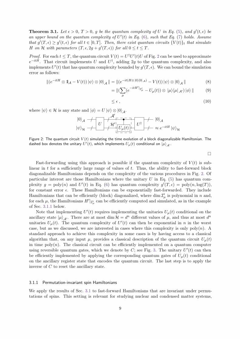
Theorem 3.1. Let ε > 0, T > 0, g be the quantum complexity of U in Eq. (5), and g′(t, ε) bean upper bound on the quantum complexity of U ′(t) in Eq. (6), such that Eq. (7) holds. Assumethat g′(T, ε) ≥ g′(t, ε) for all t ∈ [0, T ]. Then, there exist quantum circuits V (t)t that simulateH on H with parameters (T, ε, 2g + g′(T, ε)) for all 0 ≤ t ≤ T .

Proof. For each t ≤ T , the quantum circuit V (t) = U †U ′(t)U of Fig. 2 can be used to approximatee−itH . That circuit implements U and U †, adding 2g to the quantum complexity, and alsoimplements U ′(t) that has quantum complexity bounded by g′(T, ε). We can bound the simulationerror as follows:

‖(e−itH ⊗ 1lA − V (t)) |ψ〉 ⊗ |0〉A ‖ = ‖(e−it(H⊗ |0〉〈0|A) − V (t)) |ψ〉 ⊗ |0〉A ‖ (8)

= ‖(∑µ

(e−itH′|I′µ − Uµ(t))⊗ |µ〉〈µ|A′) |φ〉 ‖ (9)

≤ ε , (10)

where |ψ〉 ∈ H is any state and |φ〉 = U |ψ〉 ⊗ |0〉A.

|0〉A /U

/A′

•U †

/ |0〉A|ψ〉H / /

H′Uµ(t) / ≈ e−itH |ψ〉H

Figure 2: The quantum circuit V (t) simulating the time evolution of a block diagonalizable Hamiltonian. Thedashed box denotes the unitary U ′(t), which implements Uµ(t) conditional on |µ〉A′ .

Fast-forwarding using this approach is possible if the quantum complexity of V (t) is sub-linear in t for a sufficiently large range of values of t. Thus, the ability to fast-forward blockdiagonalizable Hamiltonians depends on the complexity of the various procedures in Fig. 2. Ofparticular interest are those Hamiltonians where the unitary U in Eq. (5) has quantum com-plexity g = poly(n) and U ′(t) in Eq. (6) has quantum complexity g′(T, ε) = poly(n, log(T )),for constant error ε. These Hamiltonians can be exponentially fast-forwarded. They includeHamiltonians that can be efficiently (block) diagonalized, where dim I ′µ is polynomial in n and,for each µ, the Hamiltonians H ′|I′µ can be efficiently computed and simulated, as in the exampleof Sec. 3.1.1 below.

Note that implementing U ′(t) requires implementing the unitaries Uµ(t) conditional on theancillary state |µ〉A′ . There are at most dimH = dn different values of µ, and thus at most dn

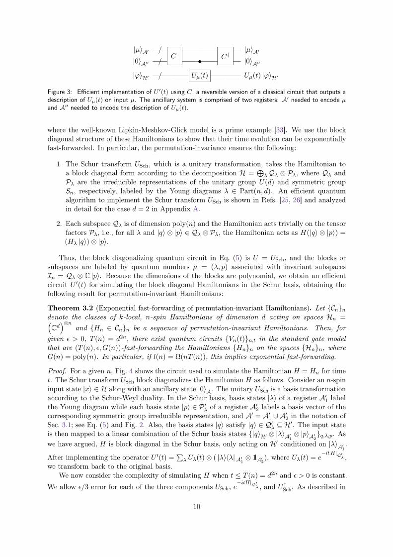
unitaries Uµ(t). The quantum complexity of U ′(t) can then be exponential in n in the worstcase, but as we discussed, we are interested in cases where this complexity is only poly(n). Astandard approach to achieve this complexity in some cases is by having access to a classicalalgorithm that, on any input µ, provides a classical description of the quantum circuit Uµ(t)in time poly(n). The classical circuit can be efficiently implemented on a quantum computerusing reversible quantum gates, which we denote by C; see Fig. 3. The unitary U ′(t) can thenbe efficiently implemented by applying the corresponding quantum gates of Uµ(t) conditionalon the ancillary register state that encodes the quantum circuit. The last step is to apply theinverse of C to reset the ancillary state.

3.1.1 Permutation-invariant spin Hamiltonians

We apply the results of Sec. 3.1 to fast-forward Hamiltonians that are invariant under permu-tations of spins. This setting is relevant for studying nuclear and condensed matter systems,

9

|µ〉A′ /C C†

|µ〉A′|0〉A′′ / • |0〉A′′

|ϕ〉H′ / Uµ(t) Uµ(t) |ϕ〉H′

Figure 3: Efficient implementation of U ′(t) using C, a reversible version of a classical circuit that outputs adescription of Uµ(t) on input µ. The ancillary system is comprised of two registers: A′ needed to encode µand A′′ needed to encode the description of Uµ(t).

where the well-known Lipkin-Meshkov-Glick model is a prime example [33]. We use the blockdiagonal structure of these Hamiltonians to show that their time evolution can be exponentiallyfast-forwarded. In particular, the permutation-invariance ensures the following:

1. The Schur transform USch, which is a unitary transformation, takes the Hamiltonian toa block diagonal form according to the decomposition H =

⊕λQλ ⊗ Pλ, where Qλ and

Pλ are the irreducible representations of the unitary group U(d) and symmetric groupSn, respectively, labeled by the Young diagrams λ ∈ Part(n, d). An efficient quantumalgorithm to implement the Schur transform USch is shown in Refs. [25, 26] and analyzedin detail for the case d = 2 in Appendix A.

2. Each subspace Qλ is of dimension poly(n) and the Hamiltonian acts trivially on the tensorfactors Pλ, i.e., for all λ and |q〉 ⊗ |p〉 ∈ Qλ ⊗ Pλ, the Hamiltonian acts as H(|q〉 ⊗ |p〉) =(Hλ |q〉)⊗ |p〉.

Thus, the block diagonalizing quantum circuit in Eq. (5) is U = USch, and the blocks orsubspaces are labeled by quantum numbers µ = (λ, p) associated with invariant subspacesIµ = Qλ ⊗ C |p〉. Because the dimensions of the blocks are polynomial, we obtain an efficientcircuit U ′(t) for simulating the block diagonal Hamiltonians in the Schur basis, obtaining thefollowing result for permutation-invariant Hamiltonians:

Theorem 3.2 (Exponential fast-forwarding of permutation-invariant Hamiltonians). Let Cnndenote the classes of k-local, n-spin Hamiltonians of dimension d acting on spaces Hn =(Cd)⊗n

and Hn ∈ Cnn be a sequence of permutation-invariant Hamiltonians. Then, forgiven ε > 0, T (n) = d2n, there exist quantum circuits Vn(t)n,t in the standard gate modelthat are (T (n), ε, G(n))-fast-forwarding the Hamiltonians Hnn on the spaces Hnn, whereG(n) = poly(n). In particular, if l(n) = Ω(nT (n)), this implies exponential fast-forwarding.

Proof. For a given n, Fig. 4 shows the circuit used to simulate the Hamiltonian H = Hn for timet. The Schur transform USch block diagonalizes the Hamiltonian H as follows. Consider an n-spininput state |x〉 ∈ H along with an ancillary state |0〉A. The unitary USch is a basis transformationaccording to the Schur-Weyl duality. In the Schur basis, basis states |λ〉 of a register A′1 labelthe Young diagram while each basis state |p〉 ∈ P ′λ of a register A′2 labels a basis vector of thecorresponding symmetric group irreducible representation, and A′ = A′1 ∪ A′2 in the notation ofSec. 3.1; see Eq. (5) and Fig. 2. Also, the basis states |q〉 satisfy |q〉 ∈ Q′λ ⊆ H′. The input stateis then mapped to a linear combination of the Schur basis states |q〉H′ ⊗ |λ〉A′1 ⊗ |p〉A′2q,λ,p. Aswe have argued, H is block diagonal in the Schur basis, only acting on H′ conditioned on |λ〉A′1 .

After implementing the operator U ′(t) =∑λ Uλ(t)⊗ ( |λ〉〈λ|A′1 ⊗ 1lA′2), where Uλ(t) = e

−itH|Q′λ ,

we transform back to the original basis.We now consider the complexity of simulating H when t ≤ T (n) = d2n and ε > 0 is constant.

We allow ε/3 error for each of the three components USch, e−itH|Q′

λ , and U †Sch. As described in

10

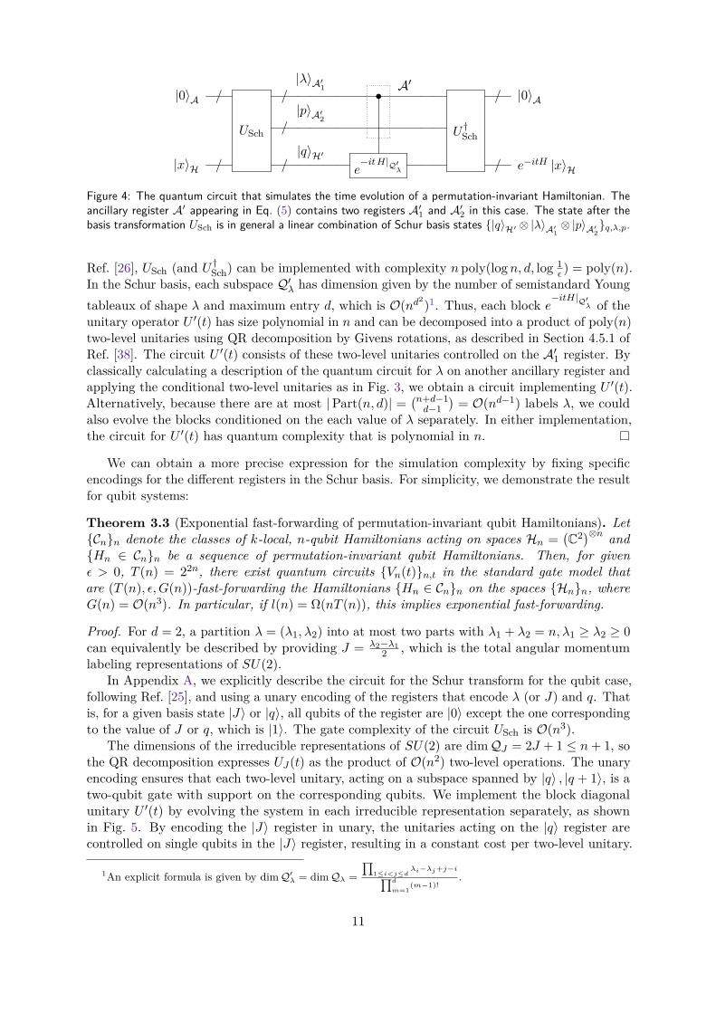
|0〉A /

USch

/

|λ〉A′1•A′

U †Sch

/ |0〉A

/

|p〉A′2

|x〉H / /|q〉H′

e−itH|Q′

λ / e−itH |x〉H

Figure 4: The quantum circuit that simulates the time evolution of a permutation-invariant Hamiltonian. Theancillary register A′ appearing in Eq. (5) contains two registers A′1 and A′2 in this case. The state after thebasis transformation USch is in general a linear combination of Schur basis states |q〉H′ ⊗ |λ〉A′1 ⊗ |p〉A′2q,λ,p.

Ref. [26], USch (and U †Sch) can be implemented with complexity n poly(logn, d, log 1ε ) = poly(n).

In the Schur basis, each subspace Q′λ has dimension given by the number of semistandard Youngtableaux of shape λ and maximum entry d, which is O(nd2)1. Thus, each block e−itH|Q′λ of theunitary operator U ′(t) has size polynomial in n and can be decomposed into a product of poly(n)two-level unitaries using QR decomposition by Givens rotations, as described in Section 4.5.1 ofRef. [38]. The circuit U ′(t) consists of these two-level unitaries controlled on the A′1 register. Byclassically calculating a description of the quantum circuit for λ on another ancillary register andapplying the conditional two-level unitaries as in Fig. 3, we obtain a circuit implementing U ′(t).Alternatively, because there are at most |Part(n, d)| =

(n+d−1d−1

)= O(nd−1) labels λ, we could

also evolve the blocks conditioned on the each value of λ separately. In either implementation,the circuit for U ′(t) has quantum complexity that is polynomial in n.

We can obtain a more precise expression for the simulation complexity by fixing specificencodings for the different registers in the Schur basis. For simplicity, we demonstrate the resultfor qubit systems:

Theorem 3.3 (Exponential fast-forwarding of permutation-invariant qubit Hamiltonians). LetCnn denote the classes of k-local, n-qubit Hamiltonians acting on spaces Hn =

(C2)⊗n and

Hn ∈ Cnn be a sequence of permutation-invariant qubit Hamiltonians. Then, for givenε > 0, T (n) = 22n, there exist quantum circuits Vn(t)n,t in the standard gate model thatare (T (n), ε, G(n))-fast-forwarding the Hamiltonians Hn ∈ Cnn on the spaces Hnn, whereG(n) = O(n3). In particular, if l(n) = Ω(nT (n)), this implies exponential fast-forwarding.

Proof. For d = 2, a partition λ = (λ1, λ2) into at most two parts with λ1 + λ2 = n, λ1 ≥ λ2 ≥ 0can equivalently be described by providing J = λ2−λ1

2 , which is the total angular momentumlabeling representations of SU(2).

In Appendix A, we explicitly describe the circuit for the Schur transform for the qubit case,following Ref. [25], and using a unary encoding of the registers that encode λ (or J) and q. Thatis, for a given basis state |J〉 or |q〉, all qubits of the register are |0〉 except the one correspondingto the value of J or q, which is |1〉. The gate complexity of the circuit USch is O(n3).

The dimensions of the irreducible representations of SU(2) are dimQJ = 2J + 1 ≤ n+ 1, sothe QR decomposition expresses UJ(t) as the product of O(n2) two-level operations. The unaryencoding ensures that each two-level unitary, acting on a subspace spanned by |q〉 , |q + 1〉, is atwo-qubit gate with support on the corresponding qubits. We implement the block diagonalunitary U ′(t) by evolving the system in each irreducible representation separately, as shownin Fig. 5. By encoding the |J〉 register in unary, the unitaries acting on the |q〉 register arecontrolled on single qubits in the |J〉 register, resulting in a constant cost per two-level unitary.

1An explicit formula is given by dim Q′λ = dim Qλ =∏

1≤i<j≤dλi−λj +j−i∏d

m=1(m−1)!

.

11

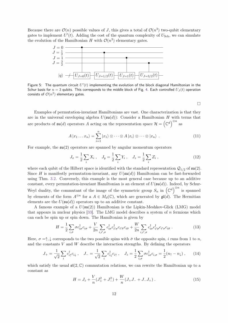
Because there are O(n) possible values of J , this gives a total of O(n3) two-qubit elementarygates to implement U ′(t). Adding the cost of the quantum complexity of USch, we can simulatethe evolution of the Hamiltonian H with O(n3) elementary gates.

J = 0 •J = 1

2 •J = 1 •J = 3

2 •

|q〉 / UJ=0(t) UJ=1/2(t) UJ=1(t) UJ=3/2(t)

Figure 5: The quantum circuit U ′(t) implementing the evolution of the block diagonal Hamiltonian in theSchur basis for n = 3 qubits. This corresponds to the middle block of Fig. 4. Each controlled UJ (t) operationconsists of O(n2) elementary gates.

Examples of permutation-invariant Hamiltonians are vast. One characterization is that theyare in the universal enveloping algebra U(su(d)): Consider a Hamiltonian H with terms thatare products of su(d) operators A acting on the representation space H =

(Cd)⊗n

as

A |x1 . . . xn〉 =n∑i=1|x1〉 ⊗ · · · ⊗A |xi〉 ⊗ · · · ⊗ |xn〉 . (11)

For example, the su(2) operators are spanned by angular momentum operators

Jx = 12∑i

Xi , Jy = 12∑i

Yi , Jz = 12∑i

Zi , (12)

where each qubit of the Hilbert space is identified with the standard representation Q1/2 of su(2).Since H is manifestly permutation-invariant, any U(su(d)) Hamiltonian can be fast-forwardedusing Thm. 3.2. Conversely, this example is the most general case because up to an additiveconstant, every permutation-invariant Hamiltonian is an element of U(su(d)). Indeed, by Schur-Weyl duality, the commutant of the image of the symmetric group Sn in

(Cd)⊗n

is spannedby elements of the form A⊗n for a A ∈ Md(C), which are generated by gl(d). The Hermitianelements are the U(su(d)) operators up to an additive constant.

A famous example of a U(su(2)) Hamiltonian is the Lipkin-Meshkov-Glick (LMG) modelthat appears in nuclear physics [33]. The LMG model describes a system of n fermions whichcan each be spin up or spin down. The Hamiltonian is given by

H = 12∑i,σ

σc†iσciσ + V

2n∑i,i′,σ

c†iσc†i′σci′σciσ + W

2n∑i,i′,σ

c†iσc†i′σci′σciσ . (13)

Here, σ =↑, ↓ corresponds to the two possible spins with σ the opposite spin, i runs from 1 to n,and the constants V and W describe the interaction strengths. By defining the operators

J+ = 1√2∑i

c†i↑ci↓ , J− = 1√2∑i

c†i↓ci↑ , Jz = 12∑i,σ

σc†iσci,σ = 12(n↑ − n↓) , (14)

which satisfy the usual sl(2,C) commutation relations, we can rewrite the Hamiltonian up to aconstant as

H = Jz + V

n(J2

+ + J2−) + W

n(J+J− + J−J+) . (15)

12

We see that H is a U(su(2)) Hamiltonian on a system of n qubits where each qubit i stores thespin of fermion i. Thus, by Thm. 3.3, the LMG model can be exponentially fast-forwarded.

3.2 Frustration-free spin Hamiltonians at low-energiesWe present a method for polynomially fast-forwarding a class of Hamiltonians denominated asfrustration-free [27, 28, 34], when the initial state is supported in a certain low-energy subspace.This setting can be relevant for studying quantum phase transitions, the simulation of adiabaticquantum state preparation, and more, where spectral gaps can decrease with the system size [22].For a spin system, a frustration-free Hamiltonian is H =

∑X⊂Λ hX , where each hX has the

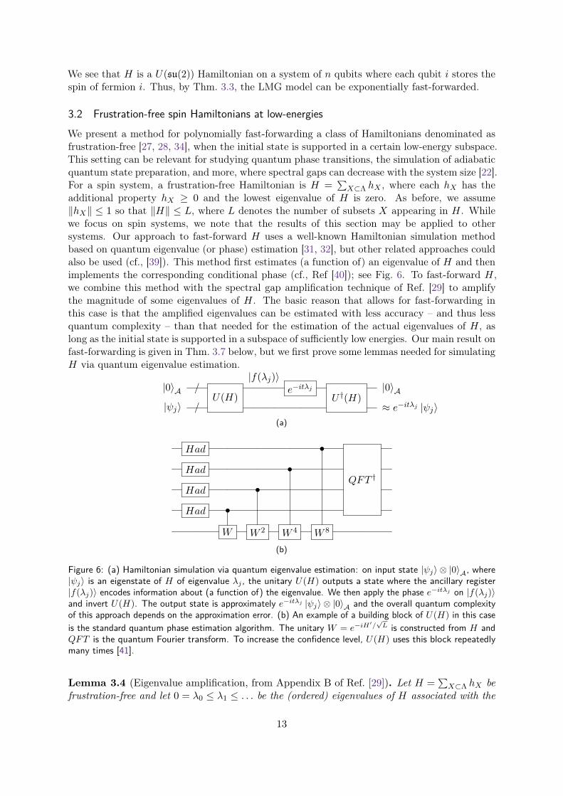
additional property hX ≥ 0 and the lowest eigenvalue of H is zero. As before, we assume‖hX‖ ≤ 1 so that ‖H‖ ≤ L, where L denotes the number of subsets X appearing in H. Whilewe focus on spin systems, we note that the results of this section may be applied to othersystems. Our approach to fast-forward H uses a well-known Hamiltonian simulation methodbased on quantum eigenvalue (or phase) estimation [31, 32], but other related approaches couldalso be used (cf., [39]). This method first estimates (a function of) an eigenvalue of H and thenimplements the corresponding conditional phase (cf., Ref [40]); see Fig. 6. To fast-forward H,we combine this method with the spectral gap amplification technique of Ref. [29] to amplifythe magnitude of some eigenvalues of H. The basic reason that allows for fast-forwarding inthis case is that the amplified eigenvalues can be estimated with less accuracy – and thus lessquantum complexity – than that needed for the estimation of the actual eigenvalues of H, aslong as the initial state is supported in a subspace of sufficiently low energies. Our main result onfast-forwarding is given in Thm. 3.7 below, but we first prove some lemmas needed for simulatingH via quantum eigenvalue estimation.

|0〉A /U(H)

|f(λj)〉e−itλj

U †(H)|0〉A

|ψj〉 / ≈ e−itλj |ψj〉(a)

Had •

QFT †Had •

Had •

Had •

W W 2 W 4 W 8

(b)

Figure 6: (a) Hamiltonian simulation via quantum eigenvalue estimation: on input state |ψj〉 ⊗ |0〉A, where|ψj〉 is an eigenstate of H of eigenvalue λj , the unitary U(H) outputs a state where the ancillary register|f(λj)〉 encodes information about (a function of) the eigenvalue. We then apply the phase e−itλj on |f(λj)〉and invert U(H). The output state is approximately e−itλj |ψj〉 ⊗ |0〉A and the overall quantum complexityof this approach depends on the approximation error. (b) An example of a building block of U(H) in this caseis the standard quantum phase estimation algorithm. The unitary W = e−iH

′/√L is constructed from H and

QFT is the quantum Fourier transform. To increase the confidence level, U(H) uses this block repeatedlymany times [41].

Lemma 3.4 (Eigenvalue amplification, from Appendix B of Ref. [29]). Let H =∑X⊂Λ hX be

frustration-free and let 0 = λ0 ≤ λ1 ≤ . . . be the (ordered) eigenvalues of H associated with the

13

eigenstates |ψj〉, j = 0, 1, . . .. Then, the Hamiltonian

H ′ =∑X⊂Λ

√hX ⊗ ( |X〉〈0|A + |0〉〈X|A) (16)

acts as the square root of H on the subspace where the ancillary state is fixed to |0〉A:

(H ′)2(|φ〉 ⊗ |0〉A) = H|φ〉 ⊗ |0〉A . (17)

The states |X〉A are orthogonal basis states (labeled by X) of an ancillary system. Furthermore,if λj > 0 and |φj〉 =

∑X⊂Λ(

√hX |ψj〉)⊗ |X〉A /λ

1/2j ,

H ′(|ψj〉 ⊗ |0〉A ± |φj〉) = ±√λj(|ψj〉 ⊗ |0〉A ± |φj〉) . (18)

The eigenvalues of H ′ are either zero or ±λ′j = ±√λj.

Thus, λ′j λj if 0 < λj 1, where eigenvalue amplification occurs. Note that each√hX

can be classically computed in constant time as this is also a k-local term and k = O(1) byassumption.

We use the method of Fig. 6 to simulate H by estimating the eigenvalues of H ′ via quantumeigenvalue estimation. If λj−1 < λj 1, then |λ′j − λ′j−1| |λj − λj−1|. Thus, we are able todemand a less accurate estimation of λ′j ’s for an accurate estimation of λj in this case:

Lemma 3.5. Let ε ≥ 0, t > 0, and ∆ > 0. Then, an estimate of an eigenvalue λj ≤ ∆ of Hwithin accuracy ε/(2t) is implied by an estimate of one of the corresponding eigenvalues ±λ′j ofH ′, defined in Eq. (16), within accuracy

δ = min√

ε

4t ,ε

8t√

∆

. (19)

Proof. The estimate of λj is obtained from the squared of the estimate of λ′j or −λ′j . Thus, itsuffices to prove

λj − ε/(2t) ≤ (λ′j ± δ)2 ≤ λj + ε/(2t) , (20)

or, equivalently, 2δ√λj + δ2 ≤ ε/(2t). We first assume δ =

√ε/(4t) ≤ ε/(8t

√∆) so that

2δ√λj + δ2 ≤ 2δ

√∆ + δ2 (21)

≤ ε/(4t) + ε/(4t) (22)≤ ε/(2t). (23)

A similar bound follows if we assume δ = ε/(8t√

∆) ≤√ε/(4t). Thus, it suffices to choose δ

according to Eq. (19) to satisfy Eq. (20).

Lemma 3.6 (Quantum eigenvalue estimation). Let H ′ be as in Eq. (16). Then, there existsa quantum circuit U(H) that, acting on input |ψj〉 ⊗ |0〉A, outputs an estimate of λ′j withinaccuracy δ and probability c ≥ 1− ε/2 after a simple measurement. The quantum complexity ofU(H) is

O(log(1/ε)L2/δ

). (24)

The O notation hides logarithmic factors in L, 1/δ, and log(1/ε).

14

Proof. The result follows from previous works. In particular, we can use the high-confidencequantum phase estimation algorithm of Ref. [41]. Let W = e−iH

′/√L be a unitary operator (note

that ‖H ′‖ ≤√L). On input |ψj〉 ⊗ |0〉A, that algorithm outputs either λ′j/

√L or −λ′j/

√L with

probability greater or equal than 1− ε/2 and within accuracy δ/√L after a simple projective

measurement. This is because |ψj〉 ⊗ |0〉A is a superposition of eigenstates of H ′ of eigenvalues±λ′j . The quantum complexity of quantum phase estimation is dominated by the number ofuses of W , or its conditional version, which in this case is m = O(log(1/ε)

√L/δ).

Next, we can simulate W using a known algorithm for Hamiltonian simulation. To avoidundesired overheads due to the precision factor, we consider the method of Ref. [9]; alterna-tively, we could use the method of Ref. [11]. Reference [9] implements W by implementing atruncated Taylor series of the exponential operator. That method requires a decomposition ofthe Hamiltonian as a linear combination of unitary operations. When H is a k-local, n-spinHamiltonian, and k = O(1), it is simple to write H ′ as a sum of O(L) unitaries. To this end,we encode the ancilla register of dimension L into logL qubits with binary encoding. Thisimplies that the Hamiltonian H ′ is a sum of L-many (k + logL)-local terms. Each of theseterms can be written as a sum of O(1) unitaries. For example,

√hX can be processed into

a sum of O(1) k-local unitaries. Also, |X〉〈0| + |0〉〈X| = 14(1 + Z0X)U0X(1 + Z0X), where

Z0X = |0〉〈0| + |X〉〈X| −∑Li=1:i 6=X |i〉〈i| and U0X = |X〉〈0| + |0〉〈X| +

∑Li=1:i 6=X |i〉〈i| are

logL-local unitaries. The latter can be easily expressed as products of O(logL) controlled bitand phase flips (two-qubit gates) using standard techniques [38].

Then, we use the method of Ref. [9] to simulate W . This method assumes a presentation ofthe Hamiltonian as a linear combination of unitaries. When the evolution time is 1/

√L and the

Hamiltonian is a sum of O(L) unitaries, and each is at most (k + logL)-local, with k = O(1),the quantum complexity of this method is O(L3/2 log(1/δ′)). The O notation hides logarithmicfactors in L, and δ′ is the accuracy.

The quantum circuit U(H) is the high-confidence quantum phase estimation algorithm,which is built upon repeated many calls of Fig. 6(b), and where W is approximated as above.The result then follows by noticing that it suffices to choose δ′ = O(δ/m) for overall accuracy δ.The resulting quantum complexity is

O(log(1/ε)L2/δ

), (25)

where we dropped logarithmic factors in L, 1/δ, and log(1/ε).

According to Lemma 3.6, fast-forwarding of frustration-free Hamiltonians can then occurwhen 1/δ is sublinear in t, since the conditional phase operation of Fig. 6(a) has a very mild(polylogarithmic) complexity dependence on t. This can happen if ∆ is sufficiently small; forexample, when ∆ is a decreasing function of t. The main result of this section is:

Theorem 3.7 (Polynomial fast-forwarding of frustration-free Hamiltonians at low energies). LetCnn denote the classes of k-local, n-spin Hamiltonians of dimension d acting on Hn =

(Cd)⊗n

and Hn =∑X⊂Λn hX ∈ Cn be frustration-free as above, with ‖hX‖ ≤ 1. The number of subsets

X in Hn is L(n) = poly(n). Let ε > 0, 0 < T (n) ≤ d2n, and ∆(n) ≤ 1/T (n). Consider thesubspaces Sn ⊆ Hnn where Sn is spanned by all the eigenstates of Hn of eigenvalues in [0,∆(n)].Then, there exist quantum circuits Vn(t)n,t in the standard gate model that are (T (n), ε, G(n))-fast-forwarding the Hamiltonians Hnn on subspaces Snn, where G(n) = O(L(n)2√T (n)).In particular, if l(n) = Ω(nT (n)), we obtain G(n)/l(n) = O(L2(n)/(n

√T (n))), which decreases

asymptotically with n if T (n) = Ω(L4(n)/n2).

15

Proof. The definition of fast-forwarding considers the simulation of Hn for all times 0 ≤ t ≤ T (n)and it suffices to consider the maximum T (n) to place an upper bound on the quantum complexityG(n). The simulation method we use is the one described in Fig. 6, where we first estimate theeigenvalues of H ′n to implement the conditional phase that approximates e−itλj .

Let δn = ε/(8√T (n)) <

√ε/(4T (n)) and c = 1− ε/4. Using the high-confidence version of

quantum phase estimation of Ref. [41] and building U(H) according to Lemma 3.6, the outputstate of U(H) is |ψj〉 ⊗ |f(λj)〉A when the input state is |ψj〉 ⊗ |0〉A. Here, |f(λj)〉A is a linearcombination of basis states and has the following properties: with probability at least 1− ε/4, itis supported on a subspace where the corresponding registers encode the eigenvalue λ′j of H ′within precision δn. Equivalently, with probability at least 1− ε/4, it is supported on a subspacewhere the corresponding registers encode the eigenvalue λj of H within precision ε/(2T (n));see Lemma 3.5. The conditional phase operation then introduces an error that is at mosttε/(2T (n)) ≤ ε/2. Inverting U(H) can also add an additional factor of ε/4 to the error. Thus,this approach simulates Hn for time t ≤ T (n) with overall error bounded by ε/4 + ε/2 + ε/4 = ε.The resulting circuits following this approach are the Vn(t)n,t, given in Fig. 6.

The quantum complexity for this method is dominated by that of U(H), analyzed inLemma 3.6. For constant error, this is O((L2(n))

√T (n)), where we dropped logarithmic factors

in L(n) and T (n). This complexity is sublinear in T (n). Assuming l(n) = Ω(nT (n)), thenG(n)/l(n)→ 0 for cases where, for example, T (n) is exponential in n.

The dominant factor in the scaling of G(n) in Thm. 3.7 is coming from√T (n), and we

refer to this case as “quadratic” fast-forwarding. While Thm. 3.7 focuses on the case where ∆decreases as 1/T , it is clear that if ∆ decreases as 1/Tα, for any positive α 6= 1, other types ofpolynomial fast-forwarding can result.

As mentioned in Sec. 2, while l(n) may not be known, several results in the literature stronglysuggest that l(n) = Ω(nT (n)) for T (n) ≤ d2n.

4 Fast-forwarding of fermionic and bosonic systemsQuantum systems obeying various particle statistics such as fermions or bosons play an importantrole in physics, including condensed matter and quantum field theories, quantum chemistry, andmore. In second quantization, Hamiltonians of n-mode fermionic and bosonic systems are writtenin terms of annihilation and creation operators ci, c

†i , respectively, where i = 1, . . . , n. Fermionic

operators satisfy the canonical anticommutation relations

ci, c†j = δij , (26)

ci, cj = 0 , (27)

while bosonic operators satisfy the canonical commutation relations

[ci, c†j ] = δij , (28)

[ci, cj ] = 0 . (29)

A fermionic or bosonic Hamiltonian is written as

H =∑

I⊆1,...,nhI , (30)

where each hI describes interactions among a subset I of fermionic or bosonic modes. Moreprecisely, hI is a sum of terms of the form a(c†i1)e1 . . . (c†ik)ek(cj1)f1 . . . (cjl)

fl , and a ∈ C. Due to

16

the exclusion principle, ei = fj = 1 for fermionic systems whereas ei ≥ 1 and fi ≥ 1 for bosonicsystems, for all i ≤ k and j ≤ l. The Hilbert space H is the standard Fock space with the propersymmetrization [42].

As for spin systems, we can define the degree of H to be the largest sum of the exponentse1 + · · · + ek + f1 + · · · + fl in the terms of hI and the weight of H to be the largest value ofk+ l. We will be particularly interested in those physically relevant cases where the degree andweight of H are constant and further assume |a| ≤ 1. In this context, a fermionic or bosonicHamiltonian sequence Hnn is meaningful if we can construct Hn from Hn−1 by adding aninteraction term vn that acts non-trivially on the n-th mode. Our definition of fast-forwardingalso depends on the model of quantum computation, and in this case, the fermionic and bosonicmodels are such that the elementary quantum gates have the form eiθlOl , where Ol is a fermionicor bosonic operator of bounded weight and degree and |θl| ≤ 1; see Def. 2.1. Note that thesemodels are different than the standard gate model, but a number of mappings can be used tosimulate fermionic or bosonic systems with qubit quantum computers if desired [3, 43].

Very few results in the literature can be used to address the no-fast-forwarding line forfermionic or bosonic systems. Such are the known results for local spin systems [16] that, undersome assumptions, could also be applied to this setting. (The resulting complexity bounds willbe weakened by overheads due to mappings between various models of quantum computing.)For certain classes of fermionic or bosonic systems, these results imply a quantum complexitythat is at least linear in t, in certain range. In general, we conjecture l(n) = Ω(poly(n)T (n)) forthe fermionic and bosonic systems discussed in the following sections, where T (n) = exp(Ω(n)).We will prove exponential fast-forwarding of quadratic fermionic and certain quadratic bosonicHamiltonians under this assumption, where the weight of H is at most 2. We do this by usinga Lie-algebra diagonalization approach that can be applied more generally.

4.1 Lie-algebra diagonalizationWe describe an approach for fast-forwarding Hamiltonians that are elements of a Lie algebraof small dimension. Hamiltonian simulation via diagonalization was also recently explored inRefs. [44, 45] with a focus on near term simulation of qubit Hamiltonians. Our method, whichworks for fermionic, bosonic, and other types of Hamiltonians, uses a Lie algebraic version ofthe Jacobi eigenvalue algorithm for diagonalizing matrices [46–48], which we review.

Suppose the Hamiltonian H is an element of a real compact semisimple Lie algebra g withLie group G. The Cartan-Weyl basis decomposition of the complexified Lie algebra implies

g = h⊕

⊕α∈R+

gα

, (31)

where h is the Cartan subalgebra, R+ ⊆ h∗ are the positive roots and each gα is the associatedtwo-dimensional space corresponding to the roots α and −α. Because g is compact, each Liesubalgebra generated by gα is isomorphic to su(2) and spanned by generalized Pauli elementsXα, Yα ∈ gα, Zα ∈ h with commutation relations

[Xα, Yα] = 2iZα , (32)[Yα, Zα] = 2iXα , (33)[Zα, Xα] = 2iYα . (34)

The Lie-algebra diagonalization approach is simply a sequence of su(2) rotations that eliminatethe off-diagonal elements on 2× 2 blocks gradually. In the first step we set H(0) = H. At each

17

step j ≥ 0, we write

H(j) = H(j)D +

∑α∈R+

(a(j)α Xα + b(j)α Yα). (35)

The H(j)D ∈ h term is the diagonal component of the Hamiltonian H(j). The off-diagonal coef-

ficients are a(j)α , b(j)α ∈ R and the goal is to make these small. To this end, we eliminate the

a(j)αj , b

(j)αj ’s of largest norm at each step. This is accomplished by performing the transformation

H(j) → H(j+1) = (V (j+1))†H(j)V (j+1) . (36)

The unitaries V (j) are su(2) rotations given by

V (j+1) = ei(πxXαj+πyYαj ) , (37)

where the coefficients |πx,y| ≤ π can be determined from H(j) in time polynomial in dim g; moredetails can be found in Ref. [48].

Convergence of the sequence H(j)j to a diagonal operator can be measured using thedistance from each Hamiltonian to the Cartan subalgebra, defined by the norm of the off-diagonalterms

dh(H(j)) =

8∑α∈R+

(|a(j)α |2 + |b(j)α |2

)1/2

.

Wildberger proved that this algorithm converges exponentially [46]:

Lemma 4.1 (Wildberger). Let H be an element of a real compact semisimple Lie algebra gwith Lie group G. Let l = |R+| < 1

2 dim g. Then, there is a sequence of r unitaries V (j) ∈exp(igαj ) ⊆ G such that

dh(H(r)) ≤(l − 1l

)r/2dh(H) . (38)

The Hamiltonian simulation approach via Lie-algebra diagonalization is given in Fig 7. Inprinciple, each unitary V (j) is a sequence of elementary gates in a corresponding model ofquantum computing determined by g. For simplicity, we define this model so that each V (j) isa single elementary gate of unit cost. Additionally, the value of r can be chosen so that thedesired accuracy in the diagonalization is achieved. In particular, there exists

r = O((dim g) log(1/ε)) (39)

that achieves dh(H(r)) ≤ εdh(H). The diagonal operation e−itH(r)D can be implemented with

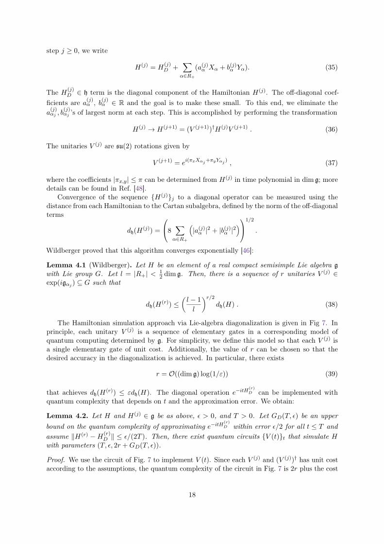
quantum complexity that depends on t and the approximation error. We obtain:

Lemma 4.2. Let H and H(j) ∈ g be as above, ε > 0, and T > 0. Let GD(T, ε) be an upperbound on the quantum complexity of approximating e−itH

(r)D within error ε/2 for all t ≤ T and

assume ‖H(r) −H(r)D ‖ ≤ ε/(2T ). Then, there exist quantum circuits V (t)t that simulate H

with parameters (T, ε, 2r +GD(T, ε)).

Proof. We use the circuit of Fig. 7 to implement V (t). Since each V (j) and (V (j))† has unit costaccording to the assumptions, the quantum complexity of the circuit in Fig. 7 is 2r plus the cost

18

of implementing e−itH(r)D . The correctness of this simulation method follows from simple norm

properties (t ≤ T ):

‖e−itH − V (1) . . . V (r)e−itH(r)D (V (r))† . . . (V (1))†‖ = ‖e−itH(r) − e−itH

(r)D ‖ (40)

≤ ‖t(H(r) −H(r)D )‖ (41)

≤ ε/2 . (42)

If, in addition, we approximate e−itH(r)D with a quantum circuit U of quantum complexity at

most GD(T, ε) such that ‖e−itH(r)D − U‖ ≤ ε/2, then the overall approximation error is bounded

by ε and the overall quantum complexity is 2r +GD(T, ε).

/ (V (1))† (V (2))† . . . (V (r))† e−itH(r)D V (r) . . . V (2) V (1)

Figure 7: Hamiltonian simulation via Lie-algebra diagonalization. The quantum circuit describes the unitaryV (t) that simulates U(t) = e−itH .

Of particular interest for fast-forwarding via Lie-algebra diagonalization is the case where lis small relative to the dimension of the Hilbert space. This occurs for many quantum systems,such as quadratic fermionic systems, where the dimension of g is only polynomial in n. In thiscase, the Lie-algebra diagonalization method described above converges quickly, and to satisfy‖H(r) −H(r)

D ‖ ≤ ε/(2T ), it suffices to choose r that is polynomial in n but only polylogarithmicin T/ε. If, in addition, the quantum complexity of approximating e−itH

(r)D within error ε is also

polynomial in n and polylogarithmic in T/ε, for t ≤ T , we attain exponential fast-forwarding:

Theorem 4.3 (Exponential fast-forwarding via Lie-algebra diagonalization). Let Cnn denoteclasses of Hamiltonians acting on spaces Hnn and Hn ∈ Cn, Hn ∈ gn, where gn is a compact,semisimple Lie algebra of dim gn = poly(n). Assume dh(Hn) = poly(n) and that, for anyX ∈ gn,

‖X −XD‖ ≤ p(n)dh(X) , dh(X) ≤ q(n)‖X −XD‖ , (43)

where p(n), q(n) = poly(n) and XD is the (diagonal) projection of X onto h. Let ε > 0 andT (n) = τn for some τ > 1. If the quantum complexity of simulating the diagonal version ofHn for time t ≤ T (n) within precision ε/2 is GD(t, ε) = poly(n, log(t‖Hn‖/ε)), then there existquantum circuits Vn(t)n,t that are (T (n), ε, G(n))-fast-forwarding the Hamiltonians Hnnon the spaces Hnn, where G(n) = poly(n). In particular, if l(n) = Ω(nT (n)), we obtainexponential fast-forwarding.

Proof. The proof is a direct consequence of Lemma 4.2 when considering the sequence of Hamil-tonians Hnn and under the assumptions on the asymptotic scalings of quantum complexities.In particular, the bounds in Eqs. (43) and dim gn = poly(n) allow us to set r = poly(n). Theclassical complexity of finding the unitaries V (j) is polynomial in the dimension of the Lie algebraand polylogarithmic in the precision, and thus is poly(n) under all the assumptions.

The requirements to achieve exponential fast-forwarding using the Lie-algebra diagonal-ization approach are satisfied by some important classes of Hamiltonians, such as quadraticfermionic and bosonic Hamiltonians, as we show below. While this diagonalization approachis efficient, in some cases it can be less efficient than directly decomposing the time evolutionoperator into a sequence of elementary quantum gates using a different approach [20, 21].

19

4.1.1 Quadratic fermionic Hamiltonians

As one example of exponential fast-forwarding via Lie-algebra diagonalization, we considerfermionic Hamiltonians which are quadratic in the creation and annihilation operators. Theseare written as

H =∑i,j

αijc†icj + βijcicj − β∗ijc

†ic†j , (44)

where we assume αij = (αji)∗, |αij | ≤ 1, and |βij | ≤ 1. Up to an additive constant, the termsin H span a compact Lie algebra g isomorphic to so(2n,R), where the Cartan subalgebra isspanned by c†ici − 1/2i [49]. This satisfies dim g = n(2n− 1), being polynomial in n, and wecan obtain a bound of the form (43). Thus we can use the analysis of the Sec. 4.1 to demonstrateexponential fast-forwarding. We obtain:

Theorem 4.4 (Exponential fast-forwarding of quadratic fermionic Hamiltonians). Let Cnndenote the classes of n-mode fermionic Hamiltonians acting on Fock spaces Hn and Hn ∈so(2n,R)n be as in Eq. (44). Let ε > 0 and T (n) = τn for some τ > 1. Then, there existquantum circuits Vn(t)n,t that are (T (n), ε, G(n))-fast-forwarding the Hamiltonians Hnn onthe spaces Hnn, where G(n) = O(n2 log(T (n))), and thus G(n) = poly(n). In particular, ifl(n) = Ω(nT (n)), we obtain exponential fast-forwarding.

Proof. The circuits Vn(t)n,t to simulate the Hamiltonians Hnn are given in Fig. 7. Forprecision ε, it suffices to choose r in Lemma 4.1 such that ‖H(r)

n −H(r)n,D‖ = O(ε/T (n)), where

H(r)n is the Hamiltonian at the r-th step of the Lie-algebra diagonalization procedure that

starts with Hn, and H(r)n,D is its projection onto the Cartan subalgebra. The elements of the

fermionic so(2n,R) algebra satisfy the bounds of Eq. (43). A precise analysis allows us to takep(n) = 1

2

√nn−1 in Eq. (43). Since |αij |, |βij | ≤ 1, the initial distance to the Cartan subalgebra is

dh(Hn) = O(n2). Thus, we choose ε = ε/(T (n)p(n)n2) in Eq. (39), and it suffices to run

r = O(

dim so(2n,R) log(T (n)p(n)n2

ε

))(45)

= O(n2 log(T (n))

)(46)

iterations of the Lie-algebra diagonalization method for each n, which determines the complexityof Vn(t). Each su(2) rotation V (j) in Fig. 7 is the exponential of a weight two fermionic operatorand is thus an elementary gate in the fermionic model of computation. Since the exponential ofthe diagonal Hamiltonian H(r)

n,D can be implemented as a sequence of O(n) rotations e−iθjc†jcj ,

|θj | ≤ π, we obtain the desired total quantum complexity G(n) = O(n2 log(T (n))).

4.1.2 Quadratic bosonic Hamiltonians

The approach of Sec. 4.1 may also be applied to quadratic bosonic Hamiltonians. However,for bosonic Hamiltonians containing non-number-conserving terms cicj , c

†ic†j , the real Lie alge-

bra spanned by the Hermitian terms is noncompact (with complexification sp(2n,C)), and theLie-algebra diagonalization technique cannot directly be used. Therefore, we consider number-conserving quadratic bosonic Hamiltonians

H =∑i,j

αijc†icj , (47)

20

where |αij | ≤ 1 and αji = α∗ij . This simplification also allows us to restrict to subspaces Sm ofm total bosons, on which H is a bounded operator. It is clear that Sm is invariant under H. Byadding a constant to H, we identify the real Lie algebra g generated by the Hermitian terms ofH as su(n), which has polynomial dimension dim g = n2− 1. The Cartan subalgebra consists ofall elements of the form

∑j γjc

†jcj where

∑j γj = 0 and γj ∈ R. Then we can use the analysis

of Sec. 4.1 to show exponential fast-forwarding.

Theorem 4.5 (Exponential fast-forwarding of number-conserving quadratic bosonic Hamiltoni-ans). Let Cnn denote the classes of n-mode, number-conserving bosonic Hamiltonians actingon Fock spaces Hn and Hn ∈ su(n)n be as in Eq. (47). Let ε > 0 and T (n) = τn for someτ > 1. Consider the subspaces Sm(n) with m(n) = poly(n). Then, there exist quantum circuitsVn(t)n,t that are (T (n), ε, G(n))-fast-forwarding the Hamiltonians Hnn on the subspacesSm(n) ⊆ Hnn, where G(n) = O(n2 log(T (n))), and thus G(n) = poly(n). In particular, ifl(n) = Ω(nT (n)), we obtain exponential fast-forwarding.

Proof. The proof is similar to that of Thm. 4.4. By restricting to the subspace Sm(n), we mayobtain bounds of the form (43), where p(n) = m(n)√

2n . Since the initial distance to the Cartansubalgebra is dh(Hn) = O(n2), we apply the Lie-algebra diagonalization method for

r = O(

dim su(n) log(T (n)p(n)n2

ε

))(48)

= O(n2 log(T (n))

)(49)

iterations. As in the fermionic case, the su(2) rotations V (j) are elementary gates and thediagonal unitary e−itH

(r)n,D can be decomposed as a sequence of O(n) rotations e−iθjc

†jcj , |θj | ≤ π.

Therefore, we obtain a total of G(n) = O(n2 log(T (n))) gates.

5 Fast-forwarding and energy measurementsWe revisit and further develop a connection between fast-forwarding and the time-energy un-certainty principle discussed in Ref. [15], using the setting described in Sec. 2. Our result,which also holds for polynomial fast-forwarding and polynomially-precise energy measurements,is roughly as follows. Suppose we can simulate a (normalized) Hamiltonian for time T usingG(T ) elementary gates. Then we can measure the eigenenergies with accuracy O(1/T ) and highconfidence using O(G(T )) elementary gates, where we dropped polylogarithmic factors in T .Conversely, suppose we can measure the eigenenergies of a Hamiltonian with accuracy δE andhigh confidence using G(δE) elementary gates. Then, we can simulate the Hamiltonian for timeO(1/δE) using O(G(δE)) elementary gates.

To prove this result, we need to provide precise definitions of energy measurements that fitwith those in Sec. 2.

Definition 5.1 (Accuracy of energy measurements). An energy measurement has accuracy δEand confidence level η > 0 if, on any input eigenstate of a Hamiltonian, we measure an outcomeE′ that satisfies

Pr(|E′ − E| ≤ δE

)≥ η , (50)

where E is the energy of the eigenstate.

21

Definition 5.2 (Parameters of energy measurements). A sequence of Hamiltonians Hnnacting on spaces Hnn has energy measurement parameters (η, δE(n), ξ, G(n)) if there existunitary operations Unn and quantum circuits Vnn that satisfy:

1. For any n and any eigenstate |ψE〉 of Hn with energy E, the unitary Un acts as

Un |ψE〉 ⊗ |0〉A = |ψE〉 ⊗∑E′

αE′ |E′〉A , (51)

and ∑E′:|E−E′|≤δE(n)

|αE′ |2 ≥ η . (52)

Therefore, a projective measurement of the ancillary system outputs an estimate E′ thatsatisfies Eq. (50).

2. For any n, the quantum circuit Vn can be implemented with at most G(n) elementary gatesand satisfies

‖(Un − Vn) |ψ〉 ⊗ |0〉A‖ ≤ ξ , (53)

for all |ψ〉 ∈ Hn.

Similarly, the sequence of Hamiltonians Hnn has energy measurement parameters(η, δE(n), ξ, G(n)) on invariant subspaces Sn ⊆ Hnn of the Hamiltonian if the two condi-tions hold for any eigenstate |ψE〉 ∈ Sn and all |ψ〉 ∈ Sn, respectively.

In the first condition, the ancillary states |E′〉A encode the energy in, for example, binaryform. Note that these definitions are essentially the same as in Ref. [15] with the addition ofG(n) for the gate count, which is necessary in our setting because we are considering a moregeneral form of efficient energy measurements.

Now we state the equivalence between fast-forwarding and energy measurements precisely.For simplicity, we restrict to qubit systems, although generalizations can be made to othermodels of computation.

Theorem 5.3 (Fast-forwarding and precise energy measurements). Let Hnn be a sequence of(qubit) Hamiltonians with norms ‖Hn‖ ≤ 1. Then the following statements hold:

1. If Hnn can be simulated with parameters (T (n), ε, G(n)), then for any constant η <1, Hnn has energy measurement parameters (η,O( 1

T (n)),O(ε log T (n)),O((log T (n))2 +G(n) log T (n))).

2. Conversely, if Hnn has energy measurement parameters (η, δE(n), ξ, G(n)), then forany constant α > 0, Hnn can be simulated with parameters (O( 1

δE(n)), αη + 2(1 − η +ξ),O(G(n))).

The same statements hold on subspaces Sn ⊆(C2)⊗n if

∥∥∥Hn|Sn∥∥∥ ≤ 1.

Proof. The proof of the theorem uses the same technique as in Ref. [15] and is reproduced inAppendix B. To prove the first statement, we use quantum phase estimation to measure theenergy. This approach requires implementing the unitaries e−itHn controlled on an ancillaryregister of O(log(T (n)) qubits and for times t ≤ T (n). To prove the second statement, wemeasure the energy E of an eigenstate |ψE〉 on an ancillary register and implement the phasee−itE on that register using standard techniques.

According to Thm. 5.3, we see that various types of fast-forwarding (e.g., polynomial) resultin various types of precise energy measurements that are not necessarily exponential.

22

6 Conclusions and outlookWe studied the problem of fast-forwarding quantum evolution in various physical settings andunder fairly general conditions, going beyond previous studies [15]. We provided a definition offast-forwarding that considers the model of quantum computation, the classes of Hamiltonians,and properties of the initial states, and used it to demonstrate exponential and polynomial fast-forwarding in quantum systems of different particle statistics. These include spin systems thathave a permutation-invariant property, frustration-free spin systems, and quadratic fermionicand bosonic systems. Our techniques could be used to demonstrate fast-forwarding of Hamilto-nians not discussed in our work. For example, although we focused on quadratic fermionic andbosonic Hamiltonians as an application of Lie-algebra diagonalization in Sec. 4.1, that methodcan be used for any Hamiltonian that is an element of a Lie algebra of small dimension; a recentresult in Ref. [45] considers a related problem.

Many open questions remain. First, we do not provide a characterization of all Hamiltoniansthat can be fast-forwarded but rather some examples. It would be interesting to understand thischaracterization better, as it has important consequences in quantum simulation and quantumcomplexity. Second, some examples of exponential fast-forwarding, such as those obtained viaLie-algebra diagonalization, are related to Hamiltonians that admit an efficient classical solution,for which spectral properties and related quantities may be computed classically efficiently [50–54]. Developing the connection between exponential fast-forwarding and efficient solvabilityfurther will be important for understanding the advantages of exponential fast-forwarding. Third,the polynomial fast-forwarding of Sec. 3.2 applies to frustration-free spin Hamiltonians, but itmight also be applied to the simulation of more general quantum field theories or other condensedmatter systems, as we are often interested in the low-energy dynamics of such Hamiltonians.Fourth, our assumptions on the no-fast-forwarding line are based on no-fast-forwarding theoremsin the literature, and extending these theorems to more general quantum systems would allowus to understand the level of fast-forwarding better when using our simulation methods. Weexpect that these and other questions will form the basis of further studies.

7 AcknowledgementsWe acknowledge support from the U.S. Department of Energy, Office of Science, High-EnergyPhysics and Office of Advanced Scientific Computing Research, under the Accelerated Researchin Quantum Computing (ARQC) program. This material is also based upon work supportedby the U.S. Department of Energy, Office of Science, National Quantum Information ScienceResearch Centers, Quantum Science Center. Los Alamos National Laboratory is managed byTriad National Security, LLC, for the National Nuclear Security Administration of the U.S.Department of Energy under Contract No. 89233218CNA000001.

23

References[1] Richard P. Feynman. Simulating physics with computers. International Journal of Theo-

retical Physics, 21(6–7):467–488, 1982. DOI: 10.1007/BF02650179.[2] Seth Lloyd. Universal quantum simulators. Science, 273(5278):1073–1078, 1996. DOI:

10.1126/science.273.5278.1073.[3] R. D. Somma, G. Ortiz, J. E. Gubernatis, E. Knill, and R. Laflamme. Simulating physical

phenomena by quantum networks. Phys. Rev. A, 65:042323, 2002. DOI: 10.1103/Phys-RevA.65.042323.

[4] D.W. Berry, G. Ahokas, R. Cleve, and B.C. Sanders. Efficient quantum algorithms forsimulating sparse Hamiltonians. Comm. Math. Phys., 270:359, 2007. DOI: 10.1007/s00220-006-0150-x.

[5] N. Wiebe, D. Berry, P. Hoyer, and B.C. Sanders. Higher order decompositions of orderedoperator exponentials. J. Phys. A: Math. Theor., 43:065203, 2010. DOI: 10.1088/1751-8113/43/6/065203.

[6] A. M. Childs and N. Wiebe. Hamiltonian simulation using linear combinations ofunitary operations. Quantum Information and Computation, 12:901–924, 2012. DOI:10.26421/QIC12.11-12-1.

[7] Dominic W. Berry and Andrew M. Childs. Black-box Hamiltonian simulation and uni-tary implementation. Quantum Information and Computation, 12(1–2):29–62, 2012. DOI:10.26421/QIC12.1-2-4. arXiv:0910.4157.

[8] Dominic W. Berry, Andrew M. Childs, Richard Cleve, Robin Kothari, and Rolando D.Somma. Exponential improvement in precision for simulating sparse Hamiltonians. InProc. of the 46th ACM Symposium on Theory of Computing, pages 283–292, 2014. DOI:10.1145/2591796.2591854.

[9] Dominic W. Berry, Andrew M. Childs, Richard Cleve, Robin Kothari, and Rolando D.Somma. Simulating Hamiltonian dynamics with a truncated Taylor series. Phys. Rev.Lett., 114:090502, 2015. DOI: 10.1103/PhysRevLett.114.090502.

[10] Dominic W. Berry, Andrew M. Childs, and Robin Kothari. Hamiltonian simulation withnearly optimal dependence on all parameters. In Proceedings of the 56th Symposium onFoundations of Computer Science, 2015. DOI: 10.1109/FOCS.2015.54.

[11] G.H. Low and I.L. Chuang. Optimal Hamiltonian simulation by quantum signal processing.Phys. Rev. Lett., 118:010501, 2017. DOI: 10.1103/PhysRevLett.118.010501.

[12] Guang Hao Low and Isaac L Chuang. Hamiltonian simulation by qubitization. Quantum,3:163, 2019. DOI: 10.22331/q-2019-07-12-163.

[13] Earl Campbell. Random compiler for fast Hamiltonian simulation. Physical review letters,123(7):070503, 2019. DOI: 10.1103/PhysRevLett.123.070503.

[14] Dominic W Berry, Andrew M Childs, Yuan Su, Xin Wang, and Nathan Wiebe. Time-dependent Hamiltonian simulation with L1-norm scaling. Quantum, 4:254, 2020. DOI:10.22331/q-2020-04-20-254.

[15] Y. Atia and D. Aharonov. Fast-forwarding of Hamiltonians and exponentially precise mea-surements. Nat. Comm., 8:1572, 2017. DOI: 10.1038/s41467-017-01637-7.

[16] Jeongwan Haah, Matthew B. Hastings, Robin Kothari, and Guang Hao Low. Quantumalgorithm for simulating real time evolution of lattice Hamiltonians. In Proceedings ofthe IEEE 59th Symposium on Foundations of Computer Science, page 350, 2018. DOI:10.1109/FOCS.2018.00041.

[17] Aram W. Harrow, Avinatan Hassidim, and Seth Lloyd. Quantum algorithm for lin-ear systems of equations. Phys. Rev. Lett., 103(15):150502, 2009. DOI: 10.1103/Phys-RevLett.103.150502.

24

[18] Andrew M. Childs, Robin Kothari, and Rolando D. Somma. Quantum linear systemsalgorithm with exponentially improved dependence on precision. SIAM J. Comp., 46:1920,2017. DOI: 10.1137/16M1087072.

[19] Frank Verstraete, J. Ignacio Cirac, and José I. Latorre. Quantum circuits for strongly corre-lated quantum systems. Phys. Rev. A, 79:032316, 2009. DOI: 10.1103/PhysRevA.79.032316.

[20] Ian D. Kivlichan, Jarrod McClean, Nathan Wiebe, Craig Gidney, Alán Aspuru-Guzik, Gar-net Kin-Lic Chan, and Ryan Babbush. Quantum simulation of electronic structure withlinear depth and connectivity. Phys. Rev. Lett., 120:110501, 2018. DOI: 10.1103/Phys-RevLett.120.110501.

[21] Zhang Jiang, Kevin J. Sung, Kostyantyn Kechedzhi, Vadim N. Smelyanskiy, and SergioBoixo. Quantum algorithms to simulate many-body physics of correlated fermions. Phys.Rev. Applied, 9:044036, 2018. DOI: 10.1103/PhysRevApplied.9.044036.

[22] Burak Şahinoğlu and Rolando D Somma. Hamiltonian simulation in the low-energy sub-space. npj Quantum Information, 7(1):1–5, 2021. DOI: 10.1038/s41534-021-00451-w.

[23] Minh C. Tran, Yuan Su, Daniel Carney, and Jacob M. Taylor. Faster digital quantum sim-ulation by symmetry protection. PRX Quantum, 2:010323, 2021. DOI: 10.1103/PRXQuan-tum.2.010323.

[24] Yuan Su, Hsin-Yuan Huang, and Earl T. Campbell. Nearly tight Trotterization of interact-ing electrons. Quantum, 5:495, 2021. DOI: 10.22331/q-2021-07-05-495.

[25] Dave Bacon, Isaac L. Chuang, and Aram W. Harrow. Efficient quantum circuits forSchur and Clebsch-Gordan transforms. Physical Review Letters, 97(17):170502, 2006. DOI:10.1103/PhysRevLett.97.170502.

[26] Dave Bacon, Isaac L. Chuang, and Aram W. Harrow. The quantum Schur transform: I.Efficient qudit circuits. arXiv:quant-ph/0601001, 2005.

[27] David Perez-Garcia, Frank Verstraete, J. Ignacio Cirac, and Michael M. Wolf. PEPS asunique ground states of local Hamiltonians. Quantum Inf. Comp., 8:0650, 2008. DOI:10.26421/QIC8.6-7-6.

[28] Sergey Bravyi and Barbara Terhal. Complexity of stoquastic frustration-free Hamiltonians.SIAM J. Comp., 39(4):1462, 2009. DOI: 10.1137/08072689X.

[29] Rolando D. Somma and Sergio Boixo. Spectral gap amplification. SIAM J. Comp, 42:593–610, 2013. DOI: 10.1137/120871997.

[30] Anirban N. Chowdhury and Rolando D. Somma. Quantum algorithms for Gibbs samplingand hitting-time estimation. Quant. Inf. Comp., 17:0041, 2017. DOI: 10.26421/QIC17.1-2-3.

[31] Alexei Y. Kitaev. Quantum measurements and the Abelian stabilizer problem. Electron.Colloquium Comput. Complex., (3), 1996.

[32] R. Cleve, A. Ekert, C. Macchiavello, and M. Mosca. Quantum algorithms revisited. Proc.R. Soc. Lond. A, 454:339–354, 1998. DOI: 10.1098/rspa.1998.0164.

[33] Harry J Lipkin, N Meshkov, and AJ Glick. Validity of many-body approximation methodsfor a solvable model: (I). Exact solutions and perturbation theory. Nuclear Physics, 62(2):188–198, 1965. DOI: 10.1016/0029-5582(65)90862-X.

[34] I. Affleck, T. Kennedy, E. H. Lieb, and H. Tasaki. Valence bond ground states in isotropicquantum antiferromagnets. Comm. Math. Phys., 115:477, 1988. DOI: 10.1007/978-3-662-06390-3_19.

[35] Stephen P Jordan, Keith SM Lee, and John Preskill. Quantum algorithms for quantumfield theories. Science, 336(6085):1130–1133, 2012. DOI: 10.1126/science.1217069.

[36] Paolo Zanardi. Symmetrizing evolutions. Physics Letters A, 258(2-3):77–82, 1999. DOI:10.1016/S0375-9601(99)00365-5.

[37] Jeremy Cook, Stephan Eidenbenz, and Andreas Bärtschi. The quantum alternatingoperator ansatz on maximum k-vertex cover. In 2020 IEEE International Confer-

25

ence on Quantum Computing and Engineering (QCE), pages 83–92. IEEE, 2020. DOI:10.1109/QCE49297.2020.00021.

[38] M. Nielsen and I. Chuang. Quantum Computation and Quantum Information. CambridgeUniversity Press, Cambridge, 2001. DOI: 10.1017/CBO9780511976667.

[39] Guang Hao Low and Isaac L Chuang. Hamiltonian simulation by qubitization. Quantum,3:163, 2019. DOI: 10.22331/q-2019-07-12-163.

[40] Andrew M Childs. On the relationship between continuous-and discrete-time quantum walk.Communications in Mathematical Physics, 294(2):581–603, 2010. DOI: 10.1007/s00220-009-0930-1.

[41] Emanuel Knill, Gerardo Ortiz, and Rolando D. Somma. Optimal quantum measurementsof expectation values of observables. Phys. Rev. A, 75:012328, 2007. DOI: 10.1103/Phys-RevA.75.012328.

[42] Michael Reed and Barry Simon. Methods of modern mathematical physics. Academic press,1978.

[43] R. D. Somma, G. Ortiz, E. Knill, and J. E. Gubernatis. Quantum simulations of physicsproblems. Int. J. Quant. Inf., 1:189, 2003. DOI: 10.1142/S0219749903000140.

[44] Cristina Cirstoiu, Zoe Holmes, Joseph Iosue, Lukasz Cincio, Patrick J Coles, and AndrewSornborger. Variational fast forwarding for quantum simulation beyond the coherence time.npj Quantum Information, 6(1):1–10, 2020. DOI: 10.1038/s41534-020-00302-0.

[45] Efekan Kökcü, Thomas Steckmann, J. K. Freericks, Eugene F. Dumitrescu, and Alexander F.Kemper. Fixed depth Hamiltonian simulation via Cartan decomposition. arXiv:2104.00728[cond-mat, physics:quant-ph], 2021.

[46] N. J. Wildberger. Diagonalization in compact lie algebras and a new proof of a theoremof kostant. Proceedings of the American Mathematical Society, 119(2):649–655, 1993. DOI:10.1090/S0002-9939-1993-1151817-6.

[47] Rolando D Somma. Quantum computation, complexity, and many-body physics. arXivquant-ph/0512209, 2005.

[48] Rolando D Somma. Unitary circuit synthesis for tomography of generalized coherent states.Journal of Mathematical Physics, 60(11):112202, 2019. DOI: 10.1063/1.5121549.

[49] Robert Gilmore and Da Hsuan Feng. Coherent states for bosons and fermions: A tutorial.Progress in Particle and Nuclear Physics, 9:479, 1983. DOI: 10.1016/0146-6410(83)90028-5.

[50] Rodney J Baxter. Exactly solved models in statistical mechanics. Elsevier, 2016. DOI:10.1142/9789814415255_0002.

[51] Vladimir E Korepin, Nicholay M Bogoliubov, and Anatoli G Izergin. Quantum inversescattering method and correlation functions, volume 3. Cambridge university press, 1997.DOI: 10.1007/BF02107233.

[52] Bill Sutherland. Beautiful models: 70 years of exactly solved quantum many-body problems.World Scientific, 2004. DOI: 10.1142/5552.

[53] Rolando Somma, Howard Barnum, Gerardo Ortiz, and Emanuel Knill. Efficient solvabilityof Hamiltonians and limits on the power of some quantum computational models. Physicalreview letters, 97(19):190501, 2006. DOI: 10.1103/PhysRevLett.97.190501.

[54] Valentin Murg, Vladimir E Korepin, and Frank Verstraete. Algebraic Bethe ansatz and ten-sor networks. Physical Review B, 86(4):045125, 2012. DOI: 10.1103/PhysRevB.86.045125.

26

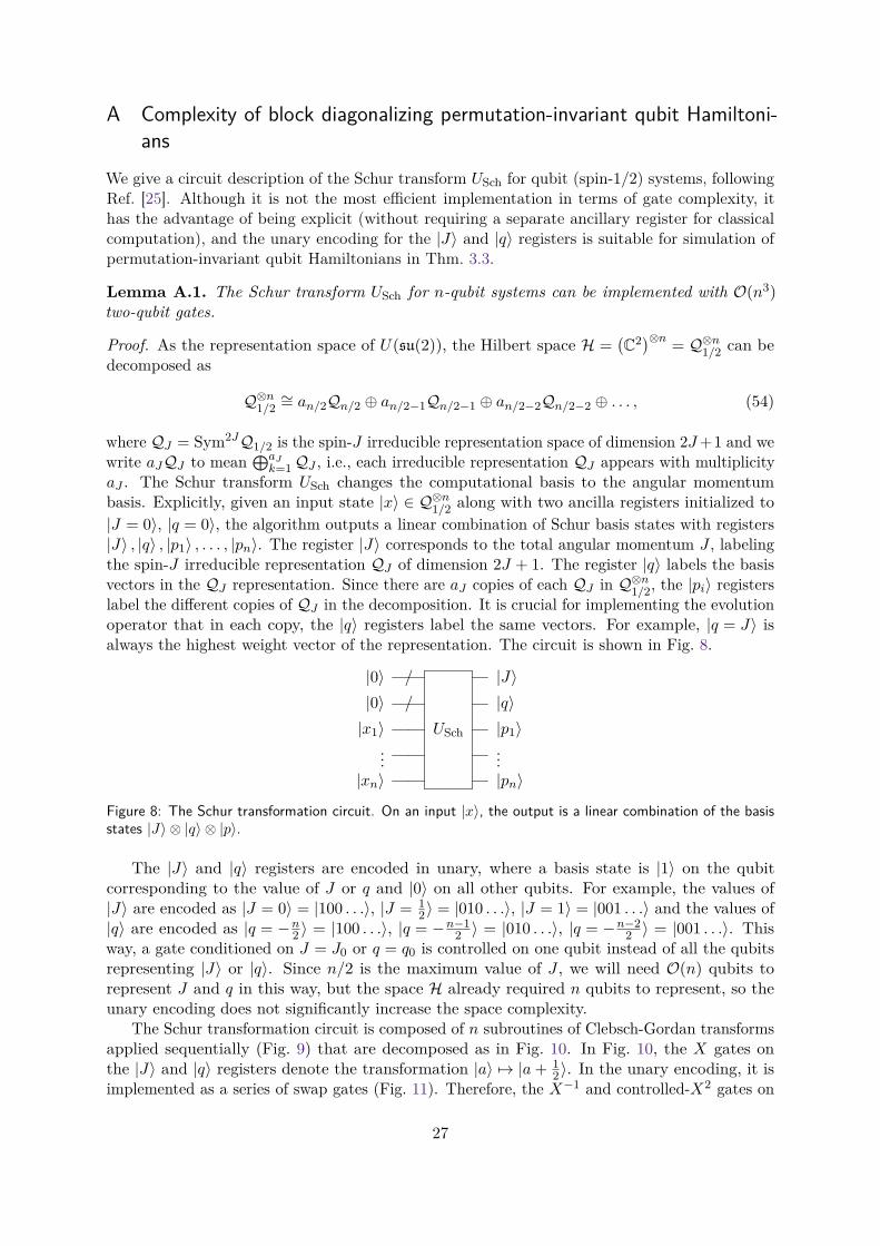
A Complexity of block diagonalizing permutation-invariant qubit Hamiltoni-ans

We give a circuit description of the Schur transform USch for qubit (spin-1/2) systems, followingRef. [25]. Although it is not the most efficient implementation in terms of gate complexity, ithas the advantage of being explicit (without requiring a separate ancillary register for classicalcomputation), and the unary encoding for the |J〉 and |q〉 registers is suitable for simulation ofpermutation-invariant qubit Hamiltonians in Thm. 3.3.

Lemma A.1. The Schur transform USch for n-qubit systems can be implemented with O(n3)two-qubit gates.

Proof. As the representation space of U(su(2)), the Hilbert space H =(C2)⊗n = Q⊗n1/2 can be

decomposed as

Q⊗n1/2∼= an/2Qn/2 ⊕ an/2−1Qn/2−1 ⊕ an/2−2Qn/2−2 ⊕ . . . , (54)

where QJ = Sym2JQ1/2 is the spin-J irreducible representation space of dimension 2J+1 and wewrite aJQJ to mean

⊕aJk=1QJ , i.e., each irreducible representation QJ appears with multiplicity

aJ . The Schur transform USch changes the computational basis to the angular momentumbasis. Explicitly, given an input state |x〉 ∈ Q⊗n1/2 along with two ancilla registers initialized to|J = 0〉, |q = 0〉, the algorithm outputs a linear combination of Schur basis states with registers|J〉 , |q〉 , |p1〉 , . . . , |pn〉. The register |J〉 corresponds to the total angular momentum J , labelingthe spin-J irreducible representation QJ of dimension 2J + 1. The register |q〉 labels the basisvectors in the QJ representation. Since there are aJ copies of each QJ in Q⊗n1/2, the |pi〉 registerslabel the different copies of QJ in the decomposition. It is crucial for implementing the evolutionoperator that in each copy, the |q〉 registers label the same vectors. For example, |q = J〉 isalways the highest weight vector of the representation. The circuit is shown in Fig. 8.

|0〉 /

USch

|J〉|0〉 / |q〉|x1〉 |p1〉

......

|xn〉 |pn〉

Figure 8: The Schur transformation circuit. On an input |x〉, the output is a linear combination of the basisstates |J〉 ⊗ |q〉 ⊗ |p〉.

The |J〉 and |q〉 registers are encoded in unary, where a basis state is |1〉 on the qubitcorresponding to the value of J or q and |0〉 on all other qubits. For example, the values of|J〉 are encoded as |J = 0〉 = |100 . . .〉, |J = 1

2〉 = |010 . . .〉, |J = 1〉 = |001 . . .〉 and the values of|q〉 are encoded as |q = −n

2 〉 = |100 . . .〉, |q = −n−12 〉 = |010 . . .〉, |q = −n−2

2 〉 = |001 . . .〉. Thisway, a gate conditioned on J = J0 or q = q0 is controlled on one qubit instead of all the qubitsrepresenting |J〉 or |q〉. Since n/2 is the maximum value of J , we will need O(n) qubits torepresent J and q in this way, but the space H already required n qubits to represent, so theunary encoding does not significantly increase the space complexity.

The Schur transformation circuit is composed of n subroutines of Clebsch-Gordan transformsapplied sequentially (Fig. 9) that are decomposed as in Fig. 10. In Fig. 10, the X gates onthe |J〉 and |q〉 registers denote the transformation |a〉 7→ |a+ 1

2〉. In the unary encoding, it isimplemented as a series of swap gates (Fig. 11). Therefore, the X−1 and controlled-X2 gates on

27

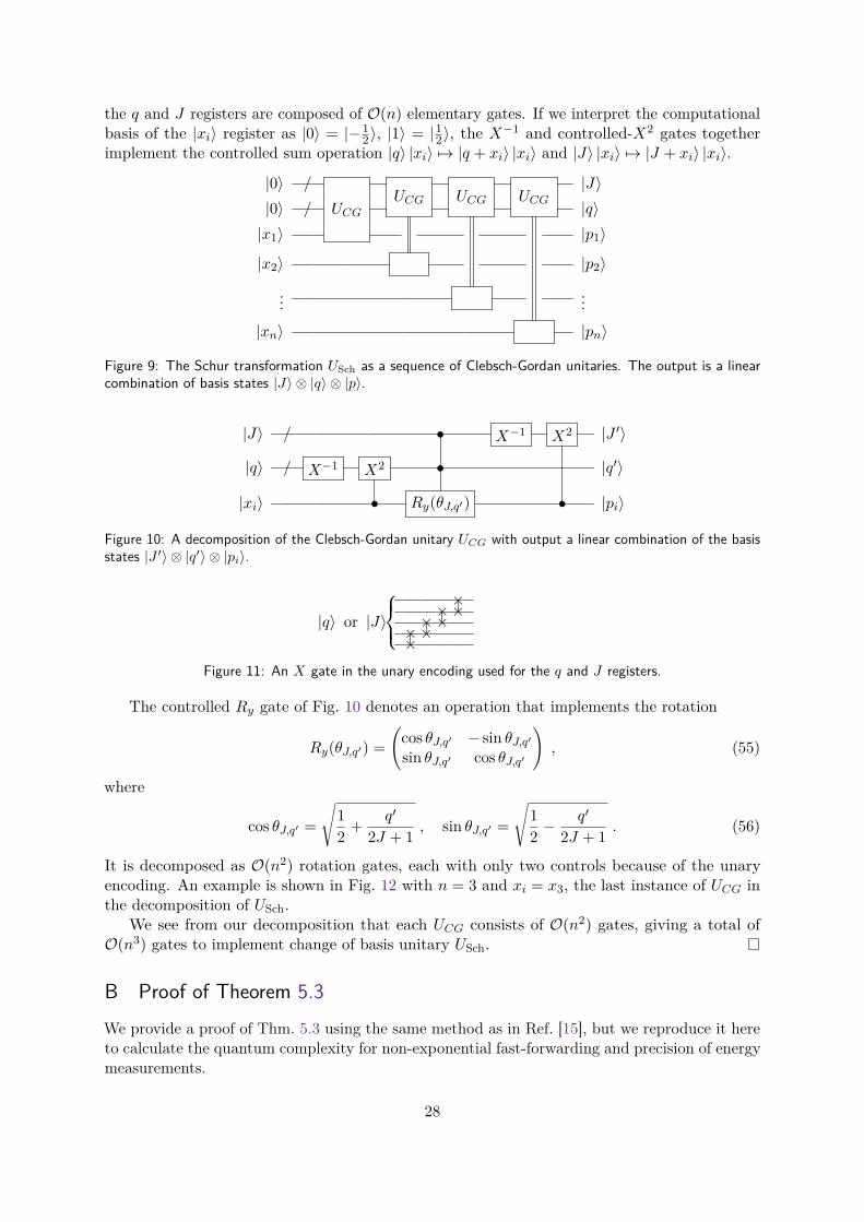
the q and J registers are composed of O(n) elementary gates. If we interpret the computationalbasis of the |xi〉 register as |0〉 = |−1

2〉, |1〉 = |12〉, the X−1 and controlled-X2 gates together

implement the controlled sum operation |q〉 |xi〉 7→ |q + xi〉 |xi〉 and |J〉 |xi〉 7→ |J + xi〉 |xi〉.

|0〉 /

UCGUCG UCG UCG

|J〉|0〉 / |q〉|x1〉 |p1〉

|x2〉 UCG |p2〉

... UCG ...|xn〉 UCG |pn〉

Figure 9: The Schur transformation USch as a sequence of Clebsch-Gordan unitaries. The output is a linearcombination of basis states |J〉 ⊗ |q〉 ⊗ |p〉.

|J〉 / • X−1 X2 |J ′〉

|q〉 / X−1 X2 • |q′〉

|xi〉 • Ry(θJ,q′) • |pi〉

Figure 10: A decomposition of the Clebsch-Gordan unitary UCG with output a linear combination of the basisstates |J ′〉 ⊗ |q′〉 ⊗ |pi〉.

×××

|q〉 or |J〉 × ××××

Figure 11: An X gate in the unary encoding used for the q and J registers.

The controlled Ry gate of Fig. 10 denotes an operation that implements the rotation

Ry(θJ,q′) =(

cos θJ,q′ − sin θJ,q′sin θJ,q′ cos θJ,q′

), (55)

where

cos θJ,q′ =

√12 + q′

2J + 1 , sin θJ,q′ =

√12 −

q′

2J + 1 . (56)

It is decomposed as O(n2) rotation gates, each with only two controls because of the unaryencoding. An example is shown in Fig. 12 with n = 3 and xi = x3, the last instance of UCG inthe decomposition of USch.

We see from our decomposition that each UCG consists of O(n2) gates, giving a total ofO(n3) gates to implement change of basis unitary USch.

B Proof of Theorem 5.3We provide a proof of Thm. 5.3 using the same method as in Ref. [15], but we reproduce it hereto calculate the quantum complexity for non-exponential fast-forwarding and precision of energymeasurements.

28

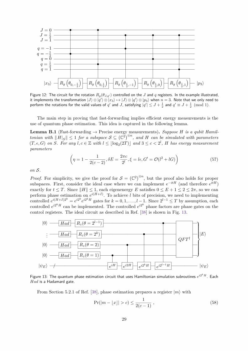
J = 0 • •J = 1

2 • • •J = 1

q = −1 •q = −1

2 •q = 0 •q = 1

2 •q = 1 •

|x3〉 Ry(θ0,− 1

2

)Ry(θ0, 1

2

)Ry(θ 1

2 ,−1

)Ry(θ 1

2 ,0

)Ry(θ 1

2 ,1

)|p3〉

Figure 12: The circuit for the rotation Ry(θJ,q′) controlled on the J and q registers. In the example illustrated,it implements the transformation |J〉 ⊗ |q′〉 ⊗ |x3〉 7→ |J〉 ⊗ |q′〉 ⊗ |p3〉 when n = 3. Note that we only need toperform the rotations for the valid values of q′ and J , satisfying |q′| ≤ J + 1

2 and q′ ≡ J + 12 (mod 1).

The main step in proving that fast-forwarding implies efficient energy measurements is theuse of quantum phase estimation. This idea is captured in the following lemma.

Lemma B.1 (Fast-forwarding → Precise energy measurements). Suppose H is a qubit Hamil-tonian with ‖H|S‖ ≤ 1 for a subspace S ⊆

(C2)⊗n, and H can be simulated with parameters

(T, ε,G) on S. For any l, c ∈ Z with l ≤ blog2(2T )c and 3 ≤ c < 2l, H has energy measurementparameters (

η = 1− 12(c− 2) , δE = 2πc

2l , ξ = lε, G′ = O(l2 + lG))

(57)

on S.

Proof. For simplicity, we give the proof for S =(C2)⊗n, but the proof also holds for proper

subspaces. First, consider the ideal case where we can implement e−itH (and therefore eitH)exactly for t ≤ T . Since ‖H‖ ≤ 1, each eigenenergy E satisfies 0 ≤ E + 1 ≤ 2 ≤ 2π, so we canperform phase estimation on ei(H+I). To achieve l bits of precision, we need to implementingcontrolled ei(H+I)2k = ei2

kei2

kH gates for k = 0, 1, . . . , l− 1. Since 2l−1 ≤ T by assumption, eachcontrolled ei2kH can be implemented. The controlled ei2k phase factors are phase gates on thecontrol registers. The ideal circuit as described in Ref. [38] is shown in Fig. 13.

|0〉 Had Rz(θ = 2l−1) •

QFT †... Had Rz(θ = 2k) • |E〉

|0〉 Had Rz(θ = 2) •

|0〉 Had Rz(θ = 1) •

|ψE〉 / eiH ei2H ei2kH ei2

l−1H |ψE〉

Figure 13: The quantum phase estimation circuit that uses Hamiltonian simulation subroutines ei2kH . EachHad is a Hadamard gate.

From Section 5.2.1 of Ref. [38], phase estimation prepares a register |m〉 with

Pr(|m− bxc| > c) ≤ 12(c− 1) , (58)

29

where c is a positive integer and x = 2l(E+12π

)for an eigenstate of energy E. Thus,

Pr(|m− x| > c) ≤ Pr(|m− bxc| > c− 1) (59)

≤ 12(c− 2) . (60)

Rearranging the left hand side gives

Pr(∣∣∣∣2πm2l − 1− E

∣∣∣∣ > 2πc2l)≤ 1

2(c− 2) , (61)

so that we have accuracy δE = 2πc2l and confidence bounded by η = 1− 1

2(c−2) .In the (nonideal) circuit, there are l Hadamard and l single qubit rotation gates, O(lG)

elementary gates from the controlled time evolution operators ei2kH , and O(l2) elementary gatesto implement the quantum Fourier transform. Therefore, the total gate count is O(l2 + lG).The error in the circuit is due to the nonideal time evolution operators from the Hamiltoniansimulation algorithm. Since each of the l instances contribute an error of at most ε, the totalerror in the energy measurement circuit is at most ξ = lε.

The converse statement that efficient energy measurements imply the ability to fast-forwardmakes use of the following lemma.

Lemma B.2 (Precise energy measurements → fast-forwarding). Suppose a qubit HamiltonianH has energy measurement parameters (η, δE, ξ,G) on a subspace S ⊆

(C2)⊗n. Then for any

T , the Hamiltonian can be simulated with parameters

(T, ε = ηδET + 2(1− η + ξ),O(G)) . (62)

on S.

Proof. Let U be the ideal energy measurement circuit and U be the approximation. In the idealcase (Fig. 14), we apply U , then apply the rotations e−itE for t ≤ T on the |E〉 register, andfinally undo the energy measurement by applying U †.

|0〉A /U

|E〉e−itE

U †|0〉A

|ψE〉 /|ψE〉

e−itE |ψE〉

Figure 14: The quantum simulation circuit using energy measurements.

When we replace U by U , there will be 2G elementary gates from the applications of U andU † and at most G gates from the rotation e−itE , since the number of ancillary qubits needed tostore the energy is at most the number of gates in the algorithm. Note that the binary encodingof |E〉 allows us to implement e−itE in parallel as individual phase gates on the |E〉 register.Thus, the total gate count is O(G).

If the energy measurement had perfect confidence η = 1 and zero error δE = 0, the idealcircuit would exactly fast-forward the Hamiltonian. The error in the actual circuit comes fromthe imperfect values of η, δE, and ξ. Denote the rotations e−itE by the unitary R. For anyeigenstate |ψE〉 of H in the subspace S, we have∥∥∥(e−itH ⊗ 1lA − U †RU) |ψE〉 ⊗ |0〉A

∥∥∥ =∥∥∥U †(e−itH ⊗ 1lA −R)U |ψE〉 ⊗ |0〉A

∥∥∥ (63)

= ‖ |ψE〉 ⊗∑E′

αE′(e−itE − e−itE′) |E′〉A ‖ (64)

≤ ηδET + 2(1− η). (65)

30

The last inequality is obtained by splitting the sum into two parts, |E′−E| ≤ δE and |E′−E| >δE. For a general state |ψ〉 =

∑E cE |ψE〉 ∈ S, the same way of splitting the sum into two parts

will give the same bound. Replacing U by U adds an additional 2ξ error. Therefore, the totalerror is α = ηδET + 2(1− η + ξ).

Combining the two lemmas, we prove Thm. 5.3.

Theorem 5.3 (Fast-forwarding and precise energy measurements). Let Hnn be a sequence of(qubit) Hamiltonians with norms ‖Hn‖ ≤ 1. Then the following statements hold:

1. If Hnn can be simulated with parameters (T (n), ε, G(n)), then for any constant η <1, Hnn has energy measurement parameters (η,O( 1

T (n)),O(ε log T (n)),O((log T (n))2 +G(n) log T (n))).

2. Conversely, if Hnn has energy measurement parameters (η, δE(n), ξ, G(n)), then forany constant α > 0, Hnn can be simulated with parameters (O( 1

δE(n)), αη + 2(1 − η +ξ),O(G(n))).

The same statements hold on subspaces Sn ⊆(C2)⊗n if

∥∥∥Hn|Sn∥∥∥ ≤ 1.

Proof. To prove the first statement, use Lemma B.1 with l = blog2(2T (n))c and c a large enoughconstant so that 1− 1

2(c−2) > η. This gives an accuracy δE(n) that is inversely proportional tothe fast-forwarding time T (n) with gate count O((log T (n))2 +G(n) log T (n)).

To prove the second statement, take T (n) = αδE(n) in Lemma B.2 to obtain fast-forwarding

for time inversely proportional to the accuracy of the measurement with gate count O(G(n)).

31