Embed Size (px)
Citation preview

Fast Equivalence Relations in Datalog
PATRICK NAPPA
SID: 440243449
Supervisor: A. Prof. Bernhard Scholz
This thesis is submitted in partial fulfillment ofthe requirements for the degree of
Bachelor of Computer Science (Adv.) (Honours)
School of Information TechnologiesThe University of Sydney
Australia
5 November 2018

Student Plagiarism: Compliance Statement
I certify that:
I have read and understood the University of Sydney Student Plagiarism: Coursework Policy and
Procedure;
I understand that failure to comply with the Student Plagiarism: Coursework Policy and Procedure
can lead to the University commencing proceedings against me for potential student misconduct under
Chapter 8 of the University of Sydney By-Law 1999 (as amended);
This Work is substantially my own, and to the extent that any part of this Work is not my own I have
indicated that it is not my own by Acknowledging the Source of that part or those parts of the Work.
Name: Patrick Nappa
Signature: Date: 26/06/2018
ii

Abstract
Declarative programs have encountered a resurgence in popularity for their ease of expression for
problems that involve large data sets; including static program analysis, security verification, network rout-
ing, and more. Of interest to efficiency, are specialised data-structures designed to increase performance
within these declarative program evaluation frameworks.
In this thesis we provide and demonstrate an efficient method for representing equivalence relations
within Datalog engines, providing at best a quadratic speed-up and space improvements. We do so via the
use of modified parallel union-find data-structures and extending the semi-naïve evaluation approach to
support these equivalence relations within the solving framework. To our understanding, this is the first
time that a self-computing data-structure is deployed in a Datalog engine, i.e., a set of rules is executed
implicitly by the data-structure.
We demonstrate the efficacy of this approach by implementing this in the SOUFFLÉ Datalog engine,
and comparing to the explicit representation of such programs in Datalog on real-world data-sets. We show
that our data-structure is able to store over a trillion tuples for a static program analysis scenario - deriving
the final result in under 4 seconds, where we believe an explicit representation of these equivalence
relations would take several years to compute.
iii

Acknowledgements
I’d like to thank my supervisor, Bernhard, for all the support, knowledge, dashing good looks,
patience, and wisdom afforded to this project. How he has coped with me over these years is beyond me.
I extend my thanks to the PLANG research group; Abdul, David, John, Lexi, Lyndon, Martin (as well
as the transient few) - for their meritorious company, presentations, and sanity checks afforded to me,
especially that of the past few months.
However, I’d like to reserve my greatest regards to the structural integrity of this building, and for the
support it has given to me thus far.
iv

CONTENTS
Student Plagiarism: Compliance Statement ii
Abstract iii
Acknowledgements iv
List of Figures vii
List of Tables xi
Chapter 1 Introduction 1
1.0.1 Contribution . . . . . . . . . . . . . . . . . . . . . . . . . . . . . . . . . . . . . . . . . . . . . . . . . . . . . . . . . . . . . . . . . 4
1.0.2 Outline . . . . . . . . . . . . . . . . . . . . . . . . . . . . . . . . . . . . . . . . . . . . . . . . . . . . . . . . . . . . . . . . . . . . . . 4
Chapter 2 Background 6
2.1 Datalog . . . . . . . . . . . . . . . . . . . . . . . . . . . . . . . . . . . . . . . . . . . . . . . . . . . . . . . . . . . . . . . . . . . . . . . . . . . 6
2.1.1 Evaluation . . . . . . . . . . . . . . . . . . . . . . . . . . . . . . . . . . . . . . . . . . . . . . . . . . . . . . . . . . . . . . . . . . . 8
2.2 Semi-naïve Evaluation . . . . . . . . . . . . . . . . . . . . . . . . . . . . . . . . . . . . . . . . . . . . . . . . . . . . . . . . . . . . . . 10
2.2.1 Rule Transformation . . . . . . . . . . . . . . . . . . . . . . . . . . . . . . . . . . . . . . . . . . . . . . . . . . . . . . . . . . 11
2.3 Equivalence Relations in Datalog . . . . . . . . . . . . . . . . . . . . . . . . . . . . . . . . . . . . . . . . . . . . . . . . . . . . 12
2.4 SOUFFLÉ Syntax . . . . . . . . . . . . . . . . . . . . . . . . . . . . . . . . . . . . . . . . . . . . . . . . . . . . . . . . . . . . . . . . . . . 14
Chapter 3 Equivalence Relations in Datalog Engine 16
3.1 Equivalence Relation Layer . . . . . . . . . . . . . . . . . . . . . . . . . . . . . . . . . . . . . . . . . . . . . . . . . . . . . . . . . 18
3.1.1 ADT . . . . . . . . . . . . . . . . . . . . . . . . . . . . . . . . . . . . . . . . . . . . . . . . . . . . . . . . . . . . . . . . . . . . . . . . 21
3.1.2 Iteration . . . . . . . . . . . . . . . . . . . . . . . . . . . . . . . . . . . . . . . . . . . . . . . . . . . . . . . . . . . . . . . . . . . . . 22
3.1.3 Cache Generation & Implementation . . . . . . . . . . . . . . . . . . . . . . . . . . . . . . . . . . . . . . . . . . . 24
3.1.4 Partitioning . . . . . . . . . . . . . . . . . . . . . . . . . . . . . . . . . . . . . . . . . . . . . . . . . . . . . . . . . . . . . . . . . . 27
3.1.5 Benchmarks . . . . . . . . . . . . . . . . . . . . . . . . . . . . . . . . . . . . . . . . . . . . . . . . . . . . . . . . . . . . . . . . . 29
3.2 Densifier . . . . . . . . . . . . . . . . . . . . . . . . . . . . . . . . . . . . . . . . . . . . . . . . . . . . . . . . . . . . . . . . . . . . . . . . . . 35
3.2.1 ADT . . . . . . . . . . . . . . . . . . . . . . . . . . . . . . . . . . . . . . . . . . . . . . . . . . . . . . . . . . . . . . . . . . . . . . . . 36
v

CONTENTS vi
3.2.2 C++ Implementation . . . . . . . . . . . . . . . . . . . . . . . . . . . . . . . . . . . . . . . . . . . . . . . . . . . . . . . . . . 41
3.2.3 Benchmarks . . . . . . . . . . . . . . . . . . . . . . . . . . . . . . . . . . . . . . . . . . . . . . . . . . . . . . . . . . . . . . . . . . 41
3.3 Disjoint Set . . . . . . . . . . . . . . . . . . . . . . . . . . . . . . . . . . . . . . . . . . . . . . . . . . . . . . . . . . . . . . . . . . . . . . . 48
3.3.1 ADT . . . . . . . . . . . . . . . . . . . . . . . . . . . . . . . . . . . . . . . . . . . . . . . . . . . . . . . . . . . . . . . . . . . . . . . . 49
3.3.2 Implementation . . . . . . . . . . . . . . . . . . . . . . . . . . . . . . . . . . . . . . . . . . . . . . . . . . . . . . . . . . . . . . . 57
3.3.3 PiggyList . . . . . . . . . . . . . . . . . . . . . . . . . . . . . . . . . . . . . . . . . . . . . . . . . . . . . . . . . . . . . . . . . . . . 62
3.3.4 Disjoint Set and PiggyList Benchmarks . . . . . . . . . . . . . . . . . . . . . . . . . . . . . . . . . . . . . . . . . 72
Chapter 4 Experiments 85
4.1 Bitcoin User Groups . . . . . . . . . . . . . . . . . . . . . . . . . . . . . . . . . . . . . . . . . . . . . . . . . . . . . . . . . . . . . . . 85
4.1.1 Input Dataset . . . . . . . . . . . . . . . . . . . . . . . . . . . . . . . . . . . . . . . . . . . . . . . . . . . . . . . . . . . . . . . . . 88
4.1.2 Datalog Programs . . . . . . . . . . . . . . . . . . . . . . . . . . . . . . . . . . . . . . . . . . . . . . . . . . . . . . . . . . . . 88
4.1.3 Results . . . . . . . . . . . . . . . . . . . . . . . . . . . . . . . . . . . . . . . . . . . . . . . . . . . . . . . . . . . . . . . . . . . . . . 90
4.1.4 Discussion . . . . . . . . . . . . . . . . . . . . . . . . . . . . . . . . . . . . . . . . . . . . . . . . . . . . . . . . . . . . . . . . . . . 97
4.2 Steensgaard Analysis . . . . . . . . . . . . . . . . . . . . . . . . . . . . . . . . . . . . . . . . . . . . . . . . . . . . . . . . . . . . . . . 97
4.2.1 Field-Sensitive Analysis . . . . . . . . . . . . . . . . . . . . . . . . . . . . . . . . . . . . . . . . . . . . . . . . . . . . . . . 98
4.2.2 Datalog Programs . . . . . . . . . . . . . . . . . . . . . . . . . . . . . . . . . . . . . . . . . . . . . . . . . . . . . . . . . . . . 100
4.2.3 Results . . . . . . . . . . . . . . . . . . . . . . . . . . . . . . . . . . . . . . . . . . . . . . . . . . . . . . . . . . . . . . . . . . . . . . 102
4.2.4 Discussion . . . . . . . . . . . . . . . . . . . . . . . . . . . . . . . . . . . . . . . . . . . . . . . . . . . . . . . . . . . . . . . . . . . 105
Chapter 5 Future Work 107
5.1 Equivalence Relation . . . . . . . . . . . . . . . . . . . . . . . . . . . . . . . . . . . . . . . . . . . . . . . . . . . . . . . . . . . . . . . 107
5.2 Sparse Mapping . . . . . . . . . . . . . . . . . . . . . . . . . . . . . . . . . . . . . . . . . . . . . . . . . . . . . . . . . . . . . . . . . . . 108
5.3 PiggyList . . . . . . . . . . . . . . . . . . . . . . . . . . . . . . . . . . . . . . . . . . . . . . . . . . . . . . . . . . . . . . . . . . . . . . . . . 109
Conclusion 110
Bibliography 111

List of Figures
1.1 Trie representation of a ternary relation in LogicBlox (Aref et al., 2015) 2
2.1 Datalog program computing the transitive closure of paths 7
2.2 Precedence graph of Datalog rules 7
2.3 Precedence graph for the rules within the Datalog program in Snippet 2.1 12
2.4 Equivalence relations may be defined via adding three rules in Datalog 12
2.5 Explicit facts are denoted in black (EDB), derived facts are in red 14
3.1 Architecture 17
3.2 Pairs of the equivalence relation 18
3.3 Disjoint sets of sparse elements 18
3.4 Disjoint sets of elements, tightly encoded 18
3.5 Resulting delta relation after the extension 19
3.6 Equivalence Cache that corresponds to the equivalence classes pictured in Figure 3.7 22
3.7 Example equivalence class partitioning 22
3.8 Total running time for a large equivalence class 31
3.9 Total resident memory for a large equivalence class 32
3.10 Total running time for small equivalence classes 33
3.11 Total resident memory for small equivalence classes 34
3.12 Simulation of densification of the sparse values {a, b, c, d} 37
3.13 Resulting state in the hash map 37
3.14 Resulting state in the dynamic array for the provided sequential operations. 37
3.15 Same key densification, single thread 43
3.16 Same key densification, two threads 43
vii

LIST OF FIGURES viii
3.17 Same key densification, four threads 43
3.18 Same key densification, eight threads 43
3.19 Unique key densification, single thread 44
3.20 Unique key densification, two threads 44
3.21 Unique key densification, four threads 45
3.22 Unique key densification, eight threads 45
3.23 Random key densification, single thread 46
3.24 Random key densification, two threads 46
3.25 Random key densification, four threads 46
3.26 Random key densification, eight threads 46
3.27 High contention key densification, single thread 47
3.28 High contention key densification, two threads 47
3.29 High contention key densification, four threads 48
3.30 High contention key densification, eight threads 48
3.31 Pre-union 50
3.32 After union(w,x) 50
3.33 After union(w, y) 50
3.34 Pre-union 51
3.35 After union(b,a) 51
3.36 After union(c, b) 51
3.37 After union(d, c) 51
3.38 Pre-union 51
3.39 After union(b,a) 51
3.40 After union(c, b) 51
3.41 After union(d, c) 51
3.42 Pre-union 52
3.43 After union(a,b) 52
3.44 After union(b,d) 52

LIST OF FIGURES ix
3.45 After union(e,c) 52
3.46 After union(f,g) 52
3.47 After union(e,f) 52
3.48 After find(g) 53
3.49 After union(d,e) 53
3.50 After find(b) 53
3.51 packed value of an element resident in index 1 58
3.52 Array representation of packed values 58
3.53 Equivalent disjoint-set forest 58
3.54 Store performance of various-sized atomic datatypes 60
3.55 Basic chunked-linked-list that has an access bottleneck 63
3.56 PiggyList with initial block size of 1; four elements have been created 64
3.57 Starting PiggyList - occupied elements are labelled in green, unused in white 66
3.58 PiggyList after index 3 has been deleted. Red is used to mark deleted elements 66
3.59 PiggyList after index 0 has been deleted 66
3.60 PiggyList after index 4 has been deleted 66
3.61 Starting PiggyList - the final used index is 6 67
3.62 The element at index 6 is moved to index 4, final advances to the last element (4) 67
3.63 The element at index 4 is moved to index 1, final advances to index 3 68
3.64 Index 5 is after the final index, so no elements are moved. We terminate as there is no more
elements in the deletion queue 68
3.65 Memory consumption for a multithreaded insertion benchmark. The number of threads in this
test is 16. 69
3.66 Probability graph of the linear dice roll function, the last t threads are guaranteed to succeed 71
3.67 Space consumption of a uniform probability Wait-free PiggyList 72
3.68 Runtime for read heavy concurrent operations 74
3.69 Runtime for equal read/write heavy concurrent operations 75
3.70 Runtime for write heavy concurrent operations 76

LIST OF FIGURES x
3.71 Mean Producer/Consumer runtime for read heavy concurrent operations 77
3.72 Mean Producer/Consumer runtime for equal read/write heavy concurrent operations 78
3.73 Mean Producer/Consumer runtime for write heavy concurrent operations 79
3.74 1 Thread Insertion 80
3.75 2 Threaded Parallel Insertion 80
3.76 4 Threaded Parallel Insertion 80
3.77 8 Threaded Parallel Thread Insertion 80
3.78 Memory consumption of a std::vector as elements are inserted 81
3.79 Memory consumption of a Locking PiggyList as elements are inserted 82
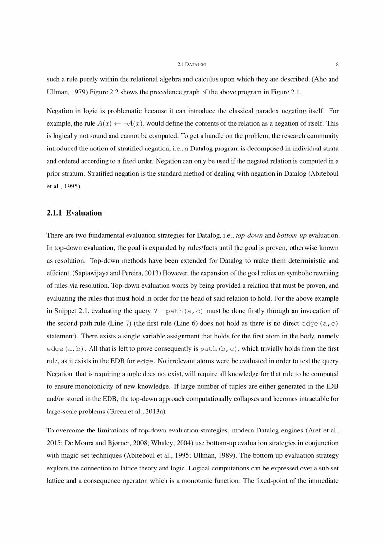
3.80 8 bit (uint8_t) append performance 83
3.81 16 bit (uint16_t) append performance 83
3.82 32 bit (uint32_t) append performance 83
3.83 64 bit (uint64_t) append performance 83
4.1 The blockchain structure (Modified from (Nakamoto, 2008)) 86
4.2 A simplified Bitcoin transaction 86
4.3 Signing a transaction with a private key (Modified from (GÃuthberg, 2006)) 87
4.4 Memory and time consumption of the input symbol table 91
4.5 Solving time for the same_user* predicate for the Bitcoin data set 92
4.6 Solving time of the implicit program vs. input tuples 93
4.7 Solving time of the explicit program vs. output tuples 94
4.8 Iteration time versus the number of output tuples 95
4.9 Memory use for both representations versus the number of input tuples 96
4.10 Resulting points-to set - field sensitive analysis 99
4.11 Solving time for various thread counts for each analysis 103
4.12 Maximum resident memory size for each analysis 105

List of Tables
4.1 Statistics of the input data set 88
4.2 Solving Time (seconds, 2 s.f.), * indicates the experiments were only ran once 92
4.3 Memory Consumption of the Bitcoin Benchmarking Programs (MB, 2 s.f.) 96
4.4 Constraint rules for the simplified field-sensitive language grammar 99
4.5 Solving time for the points-to analyses (seconds, 2 s.f.) 103
4.6 Time breakdown of the points-to analysis 104
xi

CHAPTER 1
Introduction
In recent years Datalog has emerged as domain-specific logic programming language for a wide range
of applications including static program analysis (Bravenboer and Smaragdakis, 2009), program secu-
rity (Marczak et al., 2010), program optimisations (Liu et al., 2012), cloud computing (Alvaro et al.,
2010), and networking (Loo et al., 2005). Accompanying this resurgence is a wide array of specialised
frameworks on Datalog systems that provide specialisations for various problem domains. These prob-
lems may be solved through several Datalog-based evaluation engines: LogicBlox, (Aref et al., 2015)
SOUFFLÉ , (Scholz et al., 2016) Z3, (De Moura and Bjørner, 2008) and bddbddb, (Whaley and Lam,
2004) - to name a few.
As a declarative programming language, Datalog programs are solely represented by what tasks they per-
form, rather than the low level details of how, resulting in reduced complexities in program development
and less upkeep. However, as with high-level interfaces, the programs must be sufficiently optimised
so that they are competitive with imperative implementations. These modern evaluation engines have
approached this in various ways.
Programs may be optimised at the source level, with program rewriting transformations such as Magic
Set (Ullman, 1989) that prune unnecessary computation in a Datalog program. In addition, Datalog
programs may be parallelised in that queries can be sped up via distributing work across a set of threads
or CPUs (Scholz et al., 2016; Lam et al., 2013). However, substantial performance gains can be achieved
by specialising the underlying data-structures for storing logical relations in a Datalog engine.
There has been previous successes in representing analyses using specialised data-structures in Datalog
engines. These typically take the form of a specialising Datalog engines for a given purpose. Binary
Decision Diagrams (BDDs) had been used by Whaley et al. in the bddbddb Datalog engine (Whaley,
2004) to produce the first scalable, context-sensitive, inclusion-based, (Andersen, 1994) pointer analysis
for Java programs (Whaley and Lam, 2004). Typically, these context-sensitive analyses often include call
1

1 INTRODUCTION 2
graphs with 1014 paths or more, (Whaley and Lam, 2004) and storing these explicitly would be intractable
even for smaller programs upon which are being analysed. BDDs are an efficient representation of very
large logic relations - potentially exponential in size, as is the case in context-sensitive analyses - and
enables efficient set operations between these relations. BDDs are an efficient data-structure to compress
relations in form of truth-tables. The authors noted that the performance of such generated BDD programs
were faster than the manually optimised counterparts. These BDDs are not necessarily all-encompassing -
the bddbddb tool relies on a good variable order which cannot be found in polynomial time.
LogicBlox (Aref et al., 2015) is a generalised declarative language system based on Datalog aimed at
developing enterprise software, which uses high-performance, trie data-structures to support relations
efficiently. The primary motivation for the use of tries is for computing joins between relations via their
custom Leapfrog Triejoin algorithm. This data-structure is general, in that it is not designed specifically
for a certain problem but instead provides fast performance for all interactions with the LogicBlox system.
Figure 1.1 demonstrates the space efficiency of storing tuples with many shared prefixes. This may not
be the case generally that most relations stored share the same few elements at the front of the tuple.
Performing a join in these cases is simple - iterating through all tuples with a prefix involves traversing
over the direct children. However, for cases which joins must be performed on the last element in a tuple,
this data-structure is less performant.
FIGURE 1.1: Trie representation of a ternary relation in LogicBlox (Aref et al., 2015)
LogicBlox is a popular framework for performing large-scale program analysis, performing analyses on
specifications that are not feasible for bddbddb (Bravenboer and Smaragdakis, 2009). One shortcoming
is that LogicBlox has for a single logical relation a single trie. Manual optimisations are required to

1 INTRODUCTION 3
replicate logical relations to achieve high-performance. In addition, LogicBlox evaluates these programs
in a single-threaded manner, not exploiting the ever increasing parallelism workloads of modern CPUs. It
is a proprietary system and hence not open-source.
The µZ engine is a Datalog engine in the Z3 toolbox (Hoder et al., 2011) that has been developed by
Microsoft Research. The µZ datalog engine uses a hashmap to store logical relations (Scholz et al., 2016).
Hashmaps adapt poorly to large-scale problems since their randomized memory access destroy cache
locality. However, µZ compensates the lack of fine-tuned data-structure by sophisticated source-code
level optimisations.
The design and implementation of SOUFFLÉ started at Oracle Labs in Brisbane. It was initially developed
to detect security flaws in OpenJDK. Since it was made open-source in early 2016, SOUFFLÉ has been
deployed in various applications including the analysis of networks at Amazon, and Ethereum smart
contracts. SOUFFLÉ applies code specialization ideas to generate efficient code from Datalog programs. It
builds a hierarchy of Futamura projections (Futamura, 1999) to translate Datalog program to an efficient
parallel C++ program. The data-structures for the logical relations in a program are specialized depending
on the operations that are performed. This approach diverges from prior-art: other Datalog engines use
a single data-structure for representing logical relations. As a result, SOUFFLÉ exhibits performance
characteristics that are on-par with hand-crafted state-of-the-art tools.
There is a large class of relations in Datalog programs that is a very specific case called equivalence
relations. These are binary relations that are reflexive, symmetric, and transitive. Equivalence relations
occur in various applications including points-to, network analysis, and smart-contracts to group objects.
Current Datalog engines do not use any specialised data-structures to represent equivalence relations
efficiently. A union-find data-structure (Kleinberg and Tardos, 2005) would be an appropriate choice
to represent logical equivalence relations. Instead of executing horn clauses representing properties of
equivalence relations: (1) reflexivity, (2) symmetry, and (3) transitivity; the underlying data-structure
executes these clauses implicitly. Hence, no rules need to be executed for properties (1)-(3) and the best
case compression reduction using union-find is square-root of the domain size. To achieve the integration
of a union-find data-structure in a Datalog engine, several problems arise:
(1) The semi-naïve evaluation strategy for computing the result of Datalog programs is not designed
to cope with self-computing sets. The semi-naive evaluation strategy has to be extended so that
we self-computing data-structures such as union-find can be used.

1 INTRODUCTION 4
(2) The union-find data-structure has the problem that it assumes a dense domain. This is an
obstacle for practical use because the domain of an equivalence relation are arbitrary num-
bers. A densification of the domain is required to deploy efficient union-find data-structure
implementations.
(3) Another challenge is the parallelisation of the union-find data-structure and any auxiliary data-
structures for storing logical equivalence relations. This is an essential need to harvest the
computational power of modern machines.
(4) The union-find data-structure needs to simulate the operations of a binary relations. The
implementation of a generic relation interface is required to implement these operations.
The above requirements are very challenging in terms of data-structure/algorithmic design. To show that
this is possible, we have implemented specialised equivalence relations in SOUFFLÉ . The objective was to
show that specialised data-structures for specific purposes are possible and bring substantial performance
to real-world applications.
1.0.1 Contribution
The contributions of this work are as follows:
(1) We extend the semi-naïve evaluation strategy in Datalog to accommodate for self-computing
data-structures such as union-find that perform rules implicitly.
(2) We introduce a multi-layered data-structure designed to efficiently represent equivalence rela-
tions within Datalog engines.
(3) We develop various parallel multi-threaded data-structures designed for equivalence relations.
(4) We perform extensive experiments to show the efficacy of our approach.
1.0.2 Outline
To begin, we explore relevant material to the topic of this thesis. In Chapter 2 we introduce and
formalise Datalog, investigating the evaluation strategies within both top-down and bottom Datalog
evaluation strategies and the optimisations that may be made - also covering the SOUFFLÉ environment
and equivalence relations.

1 INTRODUCTION 5
In Chapter 3, we investigate the layered data-structure, exploring the ADT interfaces, implementation
details, as well performing micro-benchmarks for each layer. Our three layers focus on iteration over
implicit pairs, transformation of a sparse domain onto a ordinal domain, and the partitioning of equivalence
classes through the union-find data-structure.
In Chapter 4 we apply real-world benchmarks to our data-structure and compare them to other approaches,
mentioning future work in Chapter 5, and concluding in Chapter 6.

CHAPTER 2
Background
2.1 Datalog
Datalog uses a fragment of first-order predicate logic(Abiteboul et al., 1995; Green et al., 2013b; Greco
and Molinaro, 2015). It restricts the model to a finite universe and rules must be phrased as Horn Clauses,
i.e., disjunctions of negated atoms with at most one positive atom. As a declarative query language,
Datalog provides a method to describe a program with regards to goals, rules, and facts. The Datalog
language lets a programmer ignore implementation details, and to focus instead on specifying what, not
how, a program evaluates.
2.1.0.1 Structure
In Datalog we differentiate between two types of logic relations. The first type of relations is called an
Extensional Database (EDB) which resembles the input of a Datalog program, i.e., the relations consists
of known facts only and have no rules. The second type of relations is called an Intensional Database
(IDB). Relations in the IDB are computed relations, i.e., their result is derived from a set of rules. The
syntax of a Datalog rule is given below:
R0 ← R1, R2, . . . , Rn.
Each Rj corresponds to a relation, which takes the form r(x0, x1, . . . , xn) for a relation with an arity
of n. Each xi is either a constant or a variable - note that the set of constants are from a finite universe.
We refer to the left-hand side of the rule as the head of the rule and we refer to the right-hand side of
the rule as the body. The body of the rule is a series of conjunctions of atoms, or simple predicates of
existence that imply the head. A rule can be interpreted as a conditional, i.e., if the body R1, . . . , Rn of a
rule holds, then then head of the rule must hold.
6

2.1 DATALOG 7
Rules without bodies are called facts, meaning that the head is unconditionally true - these are said to be
within the EDB. These are either denoted as ‘R0 ← .’, or for brevity ‘R0.’. The atoms Ri are of the form
r0(X1, X2, . . . , Xn), this captures variables X1, . . . , Xn that may be shared across atoms. The following
Datalog rule r(X) (for a variable X in the finite universe U ) is true if s(X) ∧ t(X).
r(X)← s(X), t(X).
So, if s(“string”) and t(“string”) holds, r(“string”) will consequently be true. The atom s(x) may
be true for some variable x ∈ U either through the existence of a fact s(x). within the EDB, or a rule
that describes s(x) as true as part of the IDB. We may define a goal as a rule that has no head, i.e.
← R1, . . . , Rn.. In essence, these are queries, and Datalog programs attempt to evaluate the ‘truthiness’
of goals.
2.1.0.2 Example Program
The following Datalog program describes a transitive closure over a set of edges (directed as the order
of the arguments to each predicate matter) edge(x, y). The rule path(x, y) will generate all reachable y
from x through following the set of specified edges. The following program denotes that a path between
X and Y exists if there either if there is a direct edge between X and Y , or there is a path from X to Z if
there is an edge between X and some other variable Y , and there is a path from Y to Z.
1 edge(a,b).2 edge(a,e).3 edge(b,c).4 edge(c,d).5
6 path(X,Y) ← edge(X,Y).7 path(X,Z) ← edge(X,Y), path(Y,Z).
FIGURE 2.1: Datalog programcomputing the transitive closure ofpaths
edge
path
FIGURE 2.2: Precedence graph ofDatalog rules
Datalog may contain recursive rules, which allow the above transitive closure over the set of edges to be
calculated (and concisely expressed within just two rules). Relational databases alone cannot express
2.1 DATALOG 8
such a rule purely within the relational algebra and calculus upon which they are described. (Aho and
Ullman, 1979) Figure 2.2 shows the precedence graph of the above program in Figure 2.1.
Negation in logic is problematic because it can introduce the classical paradox negating itself. For
example, the rule A(x)← ¬A(x). would define the contents of the relation as a negation of itself. This
is logically not sound and cannot be computed. To get a handle on the problem, the research community
introduced the notion of stratified negation, i.e., a Datalog program is decomposed in individual strata
and ordered according to a fixed order. Negation can only be used if the negated relation is computed in a
prior stratum. Stratified negation is the standard method of dealing with negation in Datalog (Abiteboul
et al., 1995).
2.1.1 Evaluation
There are two fundamental evaluation strategies for Datalog, i.e., top-down and bottom-up evaluation.
In top-down evaluation, the goal is expanded by rules/facts until the goal is proven, otherwise known
as resolution. Top-down methods have been extended for Datalog to make them deterministic and
efficient. (Saptawijaya and Pereira, 2013) However, the expansion of the goal relies on symbolic rewriting
of rules via resolution. Top-down evaluation works by being provided a relation that must be proven, and
evaluating the rules that must hold in order for the head of said relation to hold. For the above example
in Snippet 2.1, evaluating the query ?- path(a,c) must be done firstly through an invocation of
the second path rule (Line 7) (the first rule (Line 6) does not hold as there is no direct edge(a,c)
statement). There exists a single variable assignment that holds for the first atom in the body, namely
edge(a,b). All that is left to prove consequently is path(b,c), which trivially holds from the first
rule, as it exists in the EDB for edge. No irrelevant atoms were be evaluated in order to test the query.
Negation, that is requiring a tuple does not exist, will require all knowledge for that rule to be computed
to ensure monotonicity of new knowledge. If large number of tuples are either generated in the IDB
and/or stored in the EDB, the top-down approach computationally collapses and becomes intractable for
large-scale problems (Green et al., 2013a).
To overcome the limitations of top-down evaluation strategies, modern Datalog engines (Aref et al.,
2015; De Moura and Bjørner, 2008; Whaley, 2004) use bottom-up evaluation strategies in conjunction
with magic-set techniques (Abiteboul et al., 1995; Ullman, 1989). The bottom-up evaluation strategy
exploits the connection to lattice theory and logic. Logical computations can be expressed over a sub-set
lattice and a consequence operator, which is a monotonic function. The fixed-point of the immediate

2.1 DATALOG 9
consequence operator coincides with the result of the Datalog program; Knaster–Tarski’s (Tarski, 1955)
theorem is fundamental to make this connection work.
The immediate consequence operator TPD, for a program PD is defined as follows:(Greco and Molinaro,
2015)
TPD(I) = {A0|A0 ← A1, . . . , Anis a ground rule in ground(PD) and Ai ∈ I for every 1 ≤ i ≤ n}
This is the set of ground atoms that are generated as an immediate consequence of I w.r.t. PD, iterating
this until a fixed-point will result in the set of all computable tuples. Bottom-up evaluation involves
evaluating all captured rules in order to reach the target rule. We are able to perform some optimisations,
for example we don’t consider rules that do not reach the goal vertex in the precedence graph. The
following example demonstrates an approach of bottom-up evaluation wherein new knowledge is learned
for each iteration, although also that this approach is inefficient as tuples that already exist are re-evaluated
per step. We use the same example program shown in Figure 2.1, with path1 referring to the first rule for
path, and path2 referring to the second.
2.1.1.1 Naïve Evaluation
Using the immediate consequence operator T , we demonstrate a naïve method of solving Datalog
bottom-up. Initially, I0 contains all the ground atoms that comprise the EDB of PD as they are the
immediate consequence of no deduced knowledge, and thus can be used in the first iteration to generate
new knowledge. All previous knowledge is used to deduce further knowledge. We use the ./ operator
to denote a join across relations - i.e. this will match relations with matching terms in their arguments,
edge(a,b), path(a,c) match on the first argument, for example.
I0 = TPD(∅) = {edge(a, b), edge(a, e), edge(b, c), edge(c, d)}
I1 = TPD(I0) = I0 ./ path1 ∪ I0 ./ path2 = I0 ∪ {path(a, b), path(a, e), path(b, c), path(c, d)}
I2 = TPD(I1) = I1 ./ path1 ∪ I1 ./ path2 = I1 ∪ {path(a, c), path(b, d)}
I3 = TPD(I2) = I2 ./ path1 ∪ I2 ./ path2 = I2 ∪ {path(a, d)}
I4 = TPD(I3) = I3 ./ path1 ∪ I3 ./ path2 = I3

2.2 SEMI-NAÏVE EVALUATION 10
As I3 = I4, we have reached a fixed point, and thus there is no new knowledge to be gained. Redundant
computation is performed at each application, where all previous knowledge will be regenerated based
on the current knowledge each iteration.
Bottom-up strategies have the disadvantage that the totality of all IDB tuples are to be computed. To
reduce the amount of data in the IDB, the magic-set transformation (Bancilhon et al., 1985; Abiteboul
et al., 1995) was introduced. The transformation rewrites the Datalog program according to its goal
so that unnecessary tuples in the IDB will not be computed. We explore a more efficient method of
bottom-up evaluation, semi-naïve evaluation, in the next section.
2.2 Semi-naïve Evaluation
Naive evaluation (as demonstrated with the consequence operator) does not consider the dependencies of
the recursive relations in a Datalog program, hence, the evaluation is performed globally over all rules in
the program. With a large number of relations which may be only partially mutual recursive to each other,
the naive evaluation strategy becomes expensive. Hence, the evaluation is broken up into an evaluation
over different strata, i.e., each strata is computed in an own fixed-point, and the order of the strata is given
by the precedence graph. The other extension of the semi-naive evaluation strategy is that new tuples
in the previous iteration of the fixed-point calculations are memoized. With that “new knowledge” less
computations can be performed for gaining the new knowledge of the current iteration.
Semi-Naive evaluation was very successful in various state-of-the-art Datalog engines including Log-
icBlox (Aref et al., 2015), µZ/Z3 (Hoder et al., 2011; De Moura and Bjørner, 2008), bddbddb (Whaley,
2004), and SOUFFLÉ (Jordan et al., 2016). SOUFFLÉ is a high performance Datalog interpreter & com-
piler, converting a superset of the Datalog language to high performance, parallel C++ code. In order
to compute rules, SOUFFLÉ performs bottom-up evaluation. Rather than computing all the relations
naïvely, SOUFFLÉ uses this semi-naïve evaluation, which when sufficient program optimisations are made
to a Datalog program, will outperform or equal any top-down evaluation strategy for any query over a
program. (Ullman, 1989) Semi-naïve bottom-up evaluation is also conducive to parallelism - it is not
difficult to concurrently search for rules and perform joins across the knowledge.

2.2 SEMI-NAÏVE EVALUATION 11
2.2.1 Rule Transformation
Semi-naïve evaluation involves transforming each rule into a set of new rules. Consider the rule:
R0 ← R1, . . . , Rn.
For each Ri we may create new relations for each iteration k: Rki , and ∆Rk
i , and newRki . ∆Rk
i is an
incremental rule, it contains instances that were only exclusively newly created in iteration k, Rki denotes
the tuples of Ri known in iteration k, while newRki represents tuples that were generated in iteration k.
The new rules are constructed such that tuples will only be generated if they depend on a tuple generated
exclusively in the previous iteration, so we generate a series of rules from the original rule such that they
all involve a delta rule of the body atoms. We represent the relations using relational algebra.
For each iteration, k + 1 we solve over the following:
newRk+10 = (∆Rk
1 ./ Rk2 ./ . . . ./ R
kn)∪(Rk
1 ./ ∆Rk2 ./ . . . ./ R
kn)∪(Rk
1 ./ . . . ./ Rkn−1 ./ ∆Rk
n)\Rkn
As a result, newRk+10 contains newly derived tuples from iteration k + 1, after we have processed all the
rules for iteration k, we may update our delta rule to consist of the new knowledge derived this iteration:
∆Rk+10 = newRk+1
0 . We update the total known knowledge as Rk+10 = Rk
0 ∪ newRk+10 each iteration.
For relations with no rules in the IDB (i.e. they are only specified within the EDB), it is not necessary to
create delta rules - their set of tuples will not change which results in an empty delta each iteration, and it
is redundant to join over the empty set.
We do not simply iterate over all rules within the program within a single iteration. Semi-naïve follows
the precedence graph, in that rules should be computed after their ancestors. For recursive rules (including
mutually recursive rules), this is slightly different.
If a rule is not part of a cycle in the precedence graph (self-recursive or mutually recursive), there is no
need to compute delta knowledge, as the rule will reach a fixed point after a single iteration. For rules
that are part of a cycle in the precedence graph, only relations that are part of the SCC require delta
knowledge.
For the given Datalog program (EDB omitted) in Snippet 2.1, we demonstrate the precedence graph in
Figure 2.3, and the necessary semi-naïve rules.

2.3 EQUIVALENCE RELATIONS IN DATALOG 12
1 b(x) :- a(x).2 b(x) :- c(x,x).3 c(x,y) :- d(x,y), c(x,y).4 d(x,y) :- c(x,y).
LISTING 2.1: Example RecursiveDatalog Program
a b
c d
FIGURE 2.3: Precedence graphfor the rules within the Datalogprogram in Snippet 2.1
An example ordering may be a → {c, d} →, b. Note that c and d are solved at the same time, i.e. an
iteration will consist of deriving tuples for both c and d - this is due to their mutual recursion - generation
of facts for one may consequently generate facts for the other. We do not require special constructed
rules for a nor b. Each iteration k + 1 for solving c, d consists of iterating over the following, until a
fixed-point is reached.
newck+1 = (∆dk ./ ck) ∪ (dk ./ ∆ck) \ ck
newdk+1 = ∆ck \ dk
2.3 Equivalence Relations in Datalog
Equivalence relations are binary relations that are reflexive, symmetric, and transitive. Any elements
that are related by virtue of these properties are to be considered within the same equivalence class. As
Datalog allows concise expression of relations, it is clear that expressing equivalence relations is also
simple. We include a binary relation with equivalence relation semantics in Figure 2.4.
1 relation(a,a) :- relation(a,_). // reflexive2 relation(a,b) :- relation(b,a). // symmetric3 relation(a,c) :- relation(a,b), relation(b,c). // transitive
FIGURE 2.4: Equivalence relations may be defined via adding three rules in Datalog

2.3 EQUIVALENCE RELATIONS IN DATALOG 13
From a single tuple added, many tuples may be consequently derived. If as part of this program’s EDB,
there were the rules: relation(1,2), the consequent knowledge of relation would be:
relation(1,1),relation(1,2),relation(2,1),relation(2,2)
If the EDB also now contained relation(2,3), 5 additional tuples would be part of the final computed
knowledge:
relation(1,3),relation(2,3),relation(3,1),relation(3,2),relation(3,3)
This ‘worst-case’ behaviour is exhibited when a single large equivalence class is part of the computed
facts. In the above example, only a single equivalence class exists - E = {1, 2, 3}. If we also added in
relation(4,5) into the EDB, we would consequentially have an addition 4 facts within the computed
knowledge - the equivalence classes in the program would now be E = {{1, 2, 3}, {4, 5}}. The number
of pairs in the equivalence relation is the sum of the square of the sizes of equivalence classes within the
relation: ∑i∈E|i|2
There are multitudes of use-case scenarios for equivalence relations in Datalog, we cover two in our
real-world benchmarks (Section 4). In addition to computing Bitcoin user-groups, and Steensgaard points-
to analyses, equivalence relations can be used to compute SCCs in graphs (Suthers, 2015); must-alias
pointer analyses (Kastrinis et al., 2018); computing optimal networking routes (Thau Loo, 2010) and
more.
Snippet 2.2 demonstrates an example Datalog program that contains an equivalence relation. The EDB
consists of three facts on lines 1-3. Figure 2.5 shows the EDB facts in black edges in the graph, whilst the
derived facts are shown in red. The program defines rules and facts for whether two people live in the
same suburb.

2.4 SOUFFLÉ SYNTAX 14
1 same_suburb(alice,bob).2 same_suburb(charlie,bob).3 same_suburb(derek, eve).4
5 same_suburb(X,Y) :-same_suburb(X,_).
6 same_suburb(X,Y) :-same_suburb(Y,X).
7 same_suburb(X,Z) :-same_suburb(X,Y),
8 same_suburb(Y,Z).
LISTING 2.2: Same suburbequivalence relation in Datalog
alice
bob
charlie
derek eve
FIGURE 2.5: Explicit facts are de-noted in black (EDB), derived factsare in red
There are many derived facts in this example - from the declaration of 3 facts within the EDB, 10 facts are
evaluated as a consequence as a result from solving over the IDB (pictured in Figure 2.5 as red edges).
Any recursive evaluation strategy may require the traversing/evaluation of long paths, can result in a
number of solving iterations linear to that path length. The transitive rule of any specified equivalence
relation will incur this potential penalty.
2.4 SOUFFLÉ Syntax
SOUFFLÉ is a new Datalog engine that was designed for large-scale program analysis. The language
of SOUFFLÉ introduces a superset of Datalog containing types, functors including built-in arithmetic
predicates (such as infix addition: x + 1), aggregations (sum, average, string concatenation), records,
and more. With functors the evaluation of SOUFFLÉ programs becomes Turing complete (Keynes, 2017),
i.e., non-terminating logic programs can be constructed - this enables SOUFFLÉ to be fully-expressive. A
simple example of such a program is demonstrated in Snippet 2.3 which calculates the successor of a
number ad-infinitum.
LISTING 2.3: Non-terminating Datalog program
1 .decl succ(x : number)
2
3 succ(0).
4 succ(x+1) :- succ(x).

2.4 SOUFFLÉ SYNTAX 15
5 .output succ
In the above snippet, several important syntactical features are demonstrated:
• Types: each argument of user defined predicates uses types, which enforces type-correctness
between predicates. In this example, x is a numeric type
• Predicate Declarations: each rule defined must be declared with arity and types (line 1)
• I/O Qualifier: each predicate may be marked to output all rules to file (.output, line 5) or to
read facts in from a file (.input)
Output rules imply that all tuples for that rule must be generated - we do not specify goals in SOUFFLÉ ,
only that a relation must be fully computed. Goals can be emulated via creating a relation to be output
whose body consists of the goal to be proved. New types can also defined via the .type XXX statement.
Other functionality and syntax features are not covered in this article - the above is enough to describe all
future snippets of Datalog.

CHAPTER 3
Equivalence Relations in Datalog Engine
The major motivation of this work is to use specialised equivalence data-structure in a parallelised Datalog
engine. The specialised equivalence data-structure performs the rules for reflexivity, symmetry, and
transitivity in-situ, i.e. the rules do not need to be performed as part of the semi-naïve evaluation explicitly.
The advantage of this approach is that substantial performance gains are to be expected. For this purpose,
the Datalog engine needs to be modified so that the specialized equivalence data-structures can be used
seamlessly. There are two major undertakings in the design and implementation of equivalences. The
first undertaking is the modification of the semi-naïve evaluation approach, i.e., how can specialised
equivalence relations be used in conjunction with the semi-naïve evaluation approach. The second
undertaking is the design and implementation of a parallel equivalence data-structure for equivalence
relations that behaves like any other logical relations.
The formal definition of an equivalence relation is as follows: For elements within the domain D, an
equivalence relation may hold binary tuples R = (a, b) ∈ D × D, where the existence of tuples are
subject to the elements a and b existing within the same equivalence class. The equivalence classes is
defined as a binary relation, that is,
∀a ∈ D, (a, a) ∈ R
(a, b) ∈ R⇒ (b, a) ∈ R
for a, b, c ∈ D : (a, b), (b, c) ∈ R⇒ (a, c) ∈ R
The problem with the definition is that the domain of the binary relation could be quite large. For example,
if the binary relation is defined over the set of natural numbers. However, only a small subset of numbers
may be actually used in the concrete instance of a relation. Hence, we introduce a condensation of the
domain, i.e., we map the Datalog domain to an ordinal domain. The ordinal domain of a domain numbers
the elements of the original domain starting with zero. Hence, the ordinal domain of a domain densifies
16

3 EQUIVALENCE RELATIONS IN DATALOG ENGINE 17
the original values of the equivalence relation into dense ranges from zero to the number of elements
used in a concrete instance of a binary relation.
To efficiently express equivalence relations in Datalog, we propose a three layered data-structure for
equivalence relations. Each layer serves a purpose: The equivalence relation layer allows iteration over
the implicit pairs, insertion, and extension of tuples; the sparse mapping layer allows the storage of
sparse values efficiently; and the disjoint set layer provides a wait-free Union-Find data-structure, to store
equivalences between elements.
Equivalence Relation
Sparse Mapping
Union-Find
• Union-Find: Store elements of same re-lation in a same-set structure• Sparse Mapping: Provide value abstrac-
tion• Equivalence Relation: Allow iteration
over all equivalence tuples
FIGURE 3.1: Architecture
Pictorially - elements within the same equivalence relation are stored densely encoded, as seen in Figure
3.4, on top of which a sparse-representation of the disjoint can be formed (Figure 3.3) that requires the
storage of the following bijective mapping:
e⇔ 1, f ⇔ 5, b⇔ 4, a⇔ 3, c⇔ 2, d⇔ 0
Figure 3.2 shows the corresponding pairs of the stored equivalence relation, for each equivalence class
the number of tuples is the square of the size of the equivalence class.

3.1 EQUIVALENCE RELATION LAYER 18
(a, a)
(b, b), (b, e), (b, f), (e, b), (e, e)(e, f), (f, b), (f, e), (f, f)
(c, c), (c, d), (d, c), (d, d)
FIGURE3.2: Pairs of theequivalence rela-tion
a
e
b
c d
f
FIGURE3.3: Disjointsets of sparseelements
3
1
4
2 0
5
FIGURE3.4: Disjointsets of elements,tightly encoded
3.1 Equivalence Relation Layer
An equivalence relation provides an Abstract Data-Type (ADT) to expose all pairs in the equivalence
relation and to insert new pairs to it. The interface is designed such that it mimics the functionality of a
binary relation that is explicitly stored. The operations of the ADT are very basic. The data-structure is
composed of various layers to perform the necessary operations of the equivalence relation. The data-
structure layers contains a generic interface mimicking a generic logical relations, a Densifier (discussed
later in more detail in Section 3.2) that compresses the domain of the equivalence relation to an ordinal
domain, and a parallel union-find data-structure to partition the elements into disjoint-sets.
To accommodate semi-naïve evaluation for equivalence relations, we must extend the behaviour for the
delta relations. Delta relations contain the new knowledge learned in the previous iteration, done so in
order to reduce the number of redundant calculations, as the generation of new knowledge only occurs
when considering the most recently learned facts. However, if this delta knowledge was stored explicitly
(i.e. all pairs are stored), we would lose out on some benefits of using the implicit representation for the
underlying relation. Thus we stored this delta knowledge also as an equivalence relation.
We extend the definition of the delta operation to be an over-approximation, that is, the delta knowledge
may include pre-computed knowledge from prior iterations. This can reduce the efficiency of the semi-
naïve evaluation, and for the worst-case, revert to the performance of naïve evaluation. By treating
the delta relation as an equivalence relation, this allows efficient generation of the updated relation (i.e.
Rk+1).

3.1 EQUIVALENCE RELATION LAYER 19
Our new definition for our equivalence relation delta - ∆eqrel is:
∆eqrelRk+1i = newRk+1
i �Rki
The � operator is the extension between the two equivalence classes such that the equivalence classes are
merged. A pictograph of the resulting delta relation is demonstrated in Figure 3.5. Superfluous edges are
marked in blue, these comprise the over-approximation. Note that reflexive relations, i.e. self-loop edges
are omitted from the graph for brevity.
a
b
c
f g
d e
R k
b
f
g c
newR k+1
f
k+1 ΔR
b
a c
g
FIGURE 3.5: Resulting delta relation after the extension
These edges in the delta relation are not explicitly added during the extension step. Instead, we perform
the algorithm in 1 to extend a relation with another, also ensuring that no irrelevant classes are kept. The
equivalence class {d, e} is thus excluded from the resulting delta relation based on the example given in
Figure 3.5.
We supply the arguments Rk and newRk+1 as origR and newR respectively. Firstly, we iterate over the
new knowledge, newRk, and create elements representing each element that occur in both Rk and Rk+1.
We store these in a temporary set to ensure that we don’t cover existing elements multiple times.
For each element in this set, we add their corresponding equivalence classes into the new delta relation
for both old and new relations. We simply find the representative in that set, and insert a tuple between
that representative and the other elements within the set. This algorithm operates in amortised O(αn)

3.1 EQUIVALENCE RELATION LAYER 20
time - each element is visited at most once in each relation, where it will at most perform a constant
number of find or union queries to find the representatives of a class, or to add an edge (i.e. insert a
pair into a relation).
Algorithm 1 Return an extended relation1: procedure EXTEND(origR, newR)2: new-relation← empty relation3: element-list← empty set4: . Add elements that exist in both sets to our worklist5: for element ∈ newR do6: if element ∈ origR then7: add element to element-list8: end if9: end for
10: . add all classes from oldR that contain an element from element-list11: for element ∈ element-list do12: class← equivalence class that contains element13: for child ∈ class do14: insert (element, child) into new-relation15: . Ensure we don’t visit a class twice16: if child ∈ element-list then17: remove child from element-list18: end if19: end for20: end for21: . add all classes within newR22: for class ∈ newR do23: representative← representative of class24: for element ∈ class do25: insert (representative, element) into new-relation26: end for27: end for28: return new-relation29: end procedure
The read operations of the data-structure deals with accessing the pairs of the equivalence relations.
The access has different modes depending whether the first, the second, or both elements of the pair
are fixed. The read access itself is performed via an iterator. The iterator has the usual operations of
checking whether all tuples have been iterated (HASNEXT()), advancing to the next tuple (NEXT()),
and accessing the current tuple (GETELEMENT()).
Note that for the semi-naïve evaluation strategy, we do not need to support for simultaneous read and
write operations. The semi-naïve evaluation strategy has two distinct phases, which are entered via

3.1 EQUIVALENCE RELATION LAYER 21
barriers. These phases are alternating. The first phase may have multiple concurrent reads but no writes.
The second phase has multiple concurrent writes but no reads. This observation alleviates the design of
the data-structure and simplifies issues which would normal occur in concurrent data-structures.
3.1.1 ADT
Provided this layer is an abstraction layer, we must forward on appropriate function calls to the lower
layers, modifying them as required. We also provision an iterator interface, that is, providing methods to
call that will allow iteration over the tuples in certain fashions, or modes. SOUFFLÉ requires the support
of 4 different modes:
• ALL(): iterate over all pairs in the equivalence relation (∗, ∗)
• PREFIX(α): iterate over all pairs where the first element of the pair is fixed (α, ∗)
• SUFFIX(β): iterate over all pairs where the second element of the pair is fixed (∗, β)
• FACT(α,β): check the existence of a pair fixing both elements with concrete values (α, β)
These iterators are necessary to enable efficient joins within SOUFFLÉ . Joins can be simply performed
via finding matching tuples when elements are fixed within tuples.
We also require a PARTITION(d) function, that will provide a number of iterators that when iterated
over will explore the entire set of tuples implicitly stored within the equivalence relation. The parameter
d is a hint, whereby approximately d iterators will be returned, that cover different (in our case, disjoint,
but not necessarily the same size) portions of the tuples of the equivalence relation.
In order to modify & query the set of tuples, the following operations are also provided:
• INSERT(x,y): insert the tuple (x, y) into the equivalence relation, implicitly inserting tuples
implied by the reflexivity, symmetry, and transitivity.
• CONTAINS(x,y): return whether the tuple (x, y) exists within the equivalence relation.
• INSERTALL(other): insert all tuples contained within the relation other. We have speciali-
sations for when other is an equivalence relation.
• EXTEND(other): perform delta extension for this relation, merging the equivalence relation
other into this relation, resulting in the minimal delta equivalence relation.
• CLEAR(): reset this equivalence relation to contain no tuples, emptying it.
• SIZE(): calculate the number of tuples implicitly stored within this equivalence relation.

3.1 EQUIVALENCE RELATION LAYER 22
We will use the term anterior to refer to the first term in a tuple, whereas posterior will refer to the latter.
3.1.2 Iteration
The iterators simulate an explicitly stored binary relation. However, the equivalence relation is stored
implicitly, and as a result the algorithms for the enumeration of these binary pairs are more involved.
We fetch and store the disjoint-sets induced by the union-find data-structure into individual lists, and
upon these we iterate over. In Figure 3.6, an example iterator design is shown. We include markers for
the current list (coloured blue), and current anterior (green caret) and current posterior (red star) of the
present tuple. These lists act as a cache for the iterators to iterate over.
These lists are not necessarily ordered, either internally or externally, except they do require some
kind of iteration over them. For each iterator, there are three operations: NEXT(), HASNEXT(), and
GETELEMENT().
c d
a
f e b
* ^
FIGURE 3.6: Equivalence Cachethat corresponds to the equivalenceclasses pictured in Figure 3.7
a
e
b
c d
f
FIGURE 3.7: Example equiva-lence class partitioning
The approach for iterating over all pairs (ALL()) is simple, as seen in Algorithm 2; we advance the
posteriorIterator (red star *) until we hit the end of the list (indicated in blue). At that point, the
anteriorIterator (green caret ^) is stepped along one position. This repeats until both the anteriorIterator
and posteriorIterator reach the end of the list, at which point, we move onto the next list and reset the
anteriorIterator and posteriorIterator to point to the start of the now current list. We repeat this procedure
until we run out of lists.

3.1 EQUIVALENCE RELATION LAYER 23
Algorithm 2 Advance the iterator - ALL()1: procedure NEXT( )2: Advance posteriorIterator3: if posteriorIterator is at the end of the current list then4: Advance anteriorIterator5: if anteriorIterator is at the end of the current list then6: Advance to the next list7: if there is no next list then8: . We have no more to iterate9: return failure
10: end if11: Move anteriorIterator to the start of the current list12: end if13: Move posteriorIterator to the start of the current list14: end if15: end procedure
The logic for whether there is a next element simply checks whether stepping will cause the iterator to
overflow (reach the end of the list).
Algorithm 3 Check whether there is a next tuple - ALL()
1: procedure HASNEXT( )2: if anteriorIterator at end of current list and posteriorIterator at end of current list and there is
no next list then3: return false4: else5: return true6: end if7: end procedure
Retrieving the tuple is retrieving the elements that anteriorIterator and posteriorIterator point to, and
pack them into the front and back of a tuple, respectively.
Algorithm 4 Retrieve the current tuple from the iterator - ALL()
1: procedure GETELEMENT( )2: return (element at anteriorIterator, element at posteriorIterator)3: end procedure
For iteration over tuples in the equivalence relation with fixed anterior (PREFIX(α)), we fix both the
anteriorIterator and the current list. When the posteriorIterator reaches the end of the current list, this
marks the end of the iterator.

3.1 EQUIVALENCE RELATION LAYER 24
Algorithm 5 Advance the iterator - PREFIX(α)1: procedure NEXT( )2: Advance posteriorIterator3: if posteriorIterator is at the end of the current list then4: . We have no more to iterate5: return failure6: end if7: end procedure
Whilst the GETELEMENT() function remains the same between these two iterator modes, similar
changes must be made to the HASNEXT() predicate:
Algorithm 6 Check whether there is a next tuple - prefix(α)
1: procedure HASNEXT( )2: if posterioriterator at end of current list then3: return false4: else5: return true6: end if7: end procedure
For the SUFFIX(β) iterator, this is nearly identical. Instead, the posteriorIterator is fixed to point to the
element β, whilst the anteriorIterator now advances on successive NEXT() invocations. FACT(α,β) is
also implemented as an iterator, but both the posteriorIterator and anteriorIterator are fixed, the current
list is also static; HASNEXT() will always return false, and attempting to call NEXT() will result in
failure.
For iterators with fixed terms (as is used internally during joins), it is efficient to find the corresponding
list in practice, as the list is stored in the cache hash-map, with representatives of the equivalences classes
as keys which can be found in near constant time.
3.1.3 Cache Generation & Implementation
We apply caching as a main technique to accelerate the processing of iterators for the read-phase. Caches
are volatile, i.e., if in the next write-phase pairs are added, the caches are invalidated. Figure 3.6 shows
an abstract representation of the cache, in practice the lists are stored as values within a hash map, with
representatives (discussed further in 3.3) of the disjoint-set as the keys. We design the cache such that it

3.1 EQUIVALENCE RELATION LAYER 25
is efficient over all iterator operations, and using thread-safe data-structures such that the construction of
this cache can be performed in parallel.
Generating the cache requires only a single pass over the underlying disjoint-set. As the disjoint-set is
stored within a union-find data-structure (described further in Section 3.3) as a forest, each tree within
that forest contains a single root which is known as the representative for that set. We iterate over all
of the elements within the set, and insert that element into a list dictated by the representative of the
element’s disjoint-set, resulting in elements within the same disjoint-set being inserted into corresponding
lists. This can be done in parallel, if representative to list mapping is done via a thread-safe hash-map,
provided the list is also thread-safe.
Algorithm 7 details the general process of generating the cache. We directly interact with lower layers;
iterating over the dense values stored within the union-find data-structure (named disjoint-sets in the
following snippet), and also mapping these to their respective sparse-values via the dense to sparse
mapping in the Densifier layer (using the toSparse function).
Algorithm 7 Generate the equivalence cache
1: procedure GENERATE-CACHE( )2: for element ∈ disjoint-set do3: representative← disjoint-set.find(element)4: sparse-rep← toSparse(representative)5: sparse-element← toSparse(element)6: if sparse-rep 6∈ cache then7: cache[sparse-rep]← empty list8: end if9: cache[sparse-rep].append(sparse-element)
10: end for11: end procedure
As the above algorithm is designed to be distributed across parallel workloads, in the actual implementa-
tion we iterate over the elements by assigning threads portions of the disjoint set array to independently
iterate over. This construction is simple in OpenMP, wherein a preprocessor macro can be added to
enable this functionality. The disjoint-sets are stored within a contiguous array, where elements are
assigned indexes to represent a value. A shortened version of the parallel C++ code is provided below in
Snippet 3.1. We use the Intel TBB tbb::concurrent_hash_map (Intel, 2017) in order to provide
a thread-safe and fine-grained locking mechanism which simplifies the process for creating the list if
it does not exist already. For the list, we use a custom thread-safe random-access list, as described in
Section 3.3.3.

3.1 EQUIVALENCE RELATION LAYER 26
LISTING 3.1: C++ parallel cache generation
1 if (isCacheInvalid) {
2 const size_t sets = ds.size();
3 #pragma omp parallel for // dictate that this loop can be performed
in parallel
4 for (size_t i = 0; i < sets; ++i) {
5 size_t rep = ds.find(i);
6 size_t sparseRep = sds.toSparse(rep);
7 size_t sparseEl = sds.toSparse(i);
8
9 bool exists = cache.count(sparseRep);
10 // thread-safe list creation
11 if (!exists) {
12 // this acts as a fine grained writer’s lock
13 accessor a;
14 bool exists = cache.insert(a, sparseRep);
15 // only create the list if it doesn’t exist
16 if (!exists) a->second = make_list();
17
18 a->second->append(sparseEl);
19 } else {
20 // fine-grained reader’s lock
21 const_accessor a;
22 cache.find(a, sparseRep);
23
24 a->second->append(sparseEl);
25 }
26 }
27 cache.rehash();
28 }
We have found through internal profiling, that we observe a sub t-linear run-time improvement for t
threads. We suspect this is due to the current method of iterating over the disjoint set list as is default for
OpenMP. In this example, OpenMP uses a scheduler to assign the iterations to each thread pool (Lockman,

3.1 EQUIVALENCE RELATION LAYER 27
2013), however, by modifying the loop such that each thread worked on contiguous blocks we believe we
would see a reasonable speed-up.
The use of the isCacheInvalid variable is to only generate the cache when necessary. The cache is
designated to be stale if there has been a modifying operation on the equivalence relation - the following
set of operations invalidate the cache (and thus unconditionally setting isCacheInvalid to be true):
INSERT, INSERTALL, EXTEND, and CLEAR. If we wanted to avoid cache invalidation, this would
require being able to merge sets of lists quickly, including finding which lists to merge, which is the
purpose of the union-find data-structure as used in the lowest layer. The isCacheInvalid variable
must be atomic to prevent contending threads corrupting the stored value.
Due to the behaviour of the implemented hash-map, we must rehash the hash-map prior to iteration. In
the case of Intel’s TBB, not doing so leads to some values skipped or repeated during iteration. (Nappa,
2018)
For the size() operation, this cache generation must be performed prior. In order to calculate the
number of pairs, we must know the size of each disjoint-set. The size is simply the sum of the square of
sizes for each disjoint set. The other operations PARTITION, and iterators (ANTERIOR, etc) also
require the generation of the equivalence cache.
3.1.4 Partitioning
As the partition(count) function is designed to generate a number of iterators over the equivalence
relation (so as to allow parallel iteration over a number of threads), we require additional iterator types to
divide the number of pairs to iterate over fairly. The count argument is only meant as a guide as to how
many partitions should be created - this value is by default 400, despite the degree of parallelism usually
used by SOUFFLÉ programs being less than 64, due to the cost of sharing data across multiple socket
machines. (Scholz et al., 2016).
The new iterator CLOSURE(d) creates an iterator per disjoint set. This is beneficial as the iterator now
operates solely on a single list, is the only iterator to exist for that disjoint set. The number of pairs
covered within a CLOSURE iterator is the square of the size of that disjoint set, and can potentially be
used to divide work when the number of disjoint sets are large.

3.1 EQUIVALENCE RELATION LAYER 28
The heuristic we use for generating these partitions is simple, as demonstrated in Algorithm 8. Con-
structing the partitions is greedy - if there are too many disjoint sets there will be a single iterator over
each equivalence class (using CLOSURE), otherwise, we iterate over each equivalence class (disjoint-set),
and if it is large we split up the disjoint-set into many iterators, one for each element in the class (using
ANTERIOR). If the class is small, we generate a CLOSURE iterator for that disjoint-set. We currently do
not have the ability to group multiple equivalence classes within a single iterator.
Algorithm 8 Partition the equivalence relation to a number of iterators
1: procedure PARTITION(numIterators)2: iterators← empty list3: . Supply an iterator per equivalence class4: if number of equivalence classes ≥ numIterators then5: . Add a closure iterator for the representative of each set6: for class ∈ equivalence classes do7: rep← REPRESENTATIVE(class)8: iterators.append(CLOSURE(rep))9: end for
10: return iterators11: end if12: totalPairs← number of pairs within the equivalence relation13: for class ∈ equivalence classes do14: . if this class needs to be split up into smaller ones15: if class.size ≥ totalPairs
numIterators then16: for element ∈ class do17: iterators.append(ANTERIOR(e))18: end for19: else20: . otherwise append the closure21: rep← REPRESENTATIVE(class)22: iterators.append(CLOSURE(rep))23: end if24: end for25: return iterators26: end procedure
This partitioning is not performed in parallel - currently SOUFFLÉ operates on the expectation that the list
returned is a STL container (and as such isn’t embarrassingly parallel to work on). It would not be too
difficult to modify this to accept our concurrent list to be returned, and thus be made to work in parallel.
We believe the advantage for this approach would be most noticeable for many small disjoint-sets, or a
single large disjoint-set (where we iterate over to generate ANTERIOR iterators).

3.1 EQUIVALENCE RELATION LAYER 29
3.1.5 Benchmarks
We perform simple benchmarks to both the worst- and best-case scenarios for the data-structure. We
test two Datalog programs, one that generates a n-sized disjoint set, where the other generates n 1-sized
disjoint sets. We compare the implementation against an explicit representation for this dataset, which
uses a Binary Tree (BTree) as its underlying data-structure. This BTree is a heavily optimised thread-safe
implementation, which is used as the default data-structure for all of SOUFFLÉ ’s relations. These
benchmarks were repeated 20 times for each run.
3.1.5.1 Large Disjoint Set
For the single disjoint-set program, the version that uses our new data-structure is demonstrated in Snippet
3.2. We mark the relation mega as an equivalence relation by putting the keyword eqrel as part of
the declaration. This will now make the mega relation store its tuples within this equivalence relation
data-structure. We use the term eqrel in experiments and figures to denote the implicit representation
throughout the article.
The program is simple, we generate numbers from 1 until lim(x) (this is specified in a separate fact file),
and also the numbers lim(x) + 1 up until lim2(y) (also specified in a fact file). The .printsize
mega statement will print the size of the relation (i.e. how many tuples are stored) at the end of the
program.
LISTING 3.2: Single Set Datalog Eqrel Program
1 .decl gen1(x: number)
2 gen1(1).
3 gen1(x+1) :- gen1(x), !lim1(x).
4
5 .decl gen2(x: number)
6 gen2(x+1) :- gen2(x), !lim2(x).
7
8 .decl lim1(x : number)
9 .decl lim2(x : number)
10
11 .decl mega(x : number, y : number) eqrel
12 mega(x,y) :- gen1(x), gen2(y).

3.1 EQUIVALENCE RELATION LAYER 30
13
14 .input lim2()
15 .input lim()
16 .input gen2()
17
18 .printsize mega
If we specify lim1(4), gen2(5), and lim2(8), this will result in the following facts:
gen1→ gen1(1), gen1(2), gen1(3), gen1(4)
gen2→ gen2(5), gen2(6), gen2(7), gen2(8)
This will allow the direct generation of mega(1,5), mega(1,6), ..., mega(2,5), mega(2,6),
..., mega(4,8). Additionally, as the rule has been marked as an equivalence relation, then all the
reflexive (e.g. mega(1,1)), symmetric (mega(5,1)), and transitive rules will be added in - however
this example will not generate any rules that can exclusively be discovered through transitivity.
Snippet 3.3 is the equivalent explicit representation. Note the omitted eqrel specifier, and the additional
rules to denote reflexivity, symmetry, and transitivity. For brevity, we omit the number generator relations.
LISTING 3.3: Single Set Datalog Explicit Program
1 .decl mega_explicit(x : number, y : number)
2 mega_explicit(x,y) :- gen1(x), gen2(y).
3 mega_explicit(x,x) :- mega_explicit(x, _). // reflexive
4 mega_explicit(x,y) :- mega_explicit(y, x). // symmetric
5 mega_explicit(x,z) :- mega_explicit(x, y), mega_explicit(y, z). //
transitive
6
7 .printsize mega_explicit
We observe the running times for the ‘worst-case’ scenario in Figure 3.8.

3.1 EQUIVALENCE RELATION LAYER 31
0 50 100 150 200 250 300 350 400Number of Elements
0.0
0.1
0.2
0.3
0.4
0.5
Tim
e(s
)Single, Large Equivalence Class
Eqrel 1 ThreadEqrel 2 ThreadsEqrel 4 ThreadsEqrel 8 ThreadsExplicit 1 ThreadExplicit 2 ThreadsExplicit 4 ThreadsExplicit 8 Threads
FIGURE 3.8: Total running time for a large equivalence class
The running times for the implicit representation programs appear to grow far too slowly to be measured
accurately, for this small dataset. On the other hand, we are forced to restrict the experiment to run for
lower input ranges due to the apparent quadratic increase in running time for the explicit program.
We can see the growth in memory appears to be linear in both programs. Whilst the trend for the explicit
program shows a much steeper slope, this is not quadratic as would be expected. The data is much too
erratic to be reliably measured however, as Figure 3.9 demonstrates.

3.1 EQUIVALENCE RELATION LAYER 32
0 50 100 150 200 250 300 350 400Number of Elements
4.9
5.0
5.1
5.2
5.3
5.4
5.5
5.6M
emor
y(M
B)
Single, Large Equivalence Class
Eqrel 1 ThreadEqrel 2 ThreadsEqrel 4 ThreadsEqrel 8 ThreadsExplicit 1 ThreadExplicit 2 ThreadsExplicit 4 ThreadsExplicit 8 Threads
FIGURE 3.9: Total resident memory for a large equivalence class
We look at larger data-sets in section 4.1, where the expected quadratic memory consumption is observed.
As a result of, we have empirically shown using an explicit representation may incur a quadratic space
penalty for equivalence relations, while the implicit representation retains linear space.
3.1.5.2 Many Small Disjoint Sets
We also generate a benchmark which focuses on an example where there are no implicit pairs being
stored. Instead of generating two series of numbers and performing a cross-product, we generate a single
range, with the rule definition describing reflexivity only. We demonstrate the implicit eqrel program in
Snippet 3.4, and the explicit program in 3.5. We omit the definition of gen1.
LISTING 3.4: Many Set Datalog Implicit Program
1 .decl mega(x : number, y : number) eqrel
2 mega(x,x) :- gen1(x).

3.1 EQUIVALENCE RELATION LAYER 33
The explicit version is similar to as is the case above, the only change is the initial definition of the rule
to not include two ranges. No rule is needed to express reflexivity, as it is implied by the first rule of
mega_explicit.
LISTING 3.5: Many Set Datalog Explicit Program
1 .decl mega_explicit(x : number, y : number)
2 mega_explicit(x,x) :- gen1(x).
3 mega_explicit(x,y) :- mega_explicit(y, x).
4 mega_explicit(x,z) :- mega_explicit(x, y), mega_explicit(y, z).
20000 40000 60000 80000 100000Number elements within equivalence class
0.00
0.05
0.10
0.15
0.20
Tim
e(s
)
Isolated Equivalence Class
Eqrel (1)Eqrel (2)Eqrel (4)Eqrel (8)Explicit (1)Explicit (2)Explicit (4)Explicit (8)
FIGURE 3.10: Total running time for small equivalence classes
As expected, the solving time for the implicit equivalence relation program is slower than the explicit
representation. This test captures what would be the worst-case scenario with regards to solving time, as
there is no additional pairs stored through the implicit equivalence relation. Interestingly, the overhead in
runtime is only minor. For the implicit representation, we attribute this overhead to the cost of managing
the auxiliary data-structures, such as the sparse mapping, cache, and more.

3.1 EQUIVALENCE RELATION LAYER 34
We see that for both versions, the runtime increases as the parallelism factor increases. We are currently
unaware of the root cause or bottlenecks for this benchmark.
20000 40000 60000 80000 100000Number elements within equivalence class
20
30
40
50
60
70
80
Mem
ory
(MB
)
Isolated Equivalence Class
Eqrel (1)Eqrel (2)Eqrel (4)Eqrel (8)Explicit (1)Explicit (2)Explicit (4)Explicit (8)
FIGURE 3.11: Total resident memory for small equivalence classes
We also see that the memory overhead for the implicit program scales poorly as compared to the explicit
representation. We can attribute this to the multiple necessary hash-maps (equivalence cache, and
Densifier layer (as described later)), and other auxiliary data that requires storage, although this would
require further fine-grained profiling to confidently confirm.
Computational overhead from partitioning would also be a key contributor to the time slowdown observed
in the implicit representation. This is especially the case for the isolated equivalence classes, as a separate
iterator is generated for each of the classes which in this program is linear to the number of inputs. As
part of the generated C++ code, SOUFFLÉ will always call this partitioning, even if there is no threading
enabled (via compile-time flags). It would be worth investigating the speed-ups that may potentially be
gained if this is omitted from the generated code for single-threaded execution. Additionally, as noted
above, the partition function may be a candidate for parallelism - this would require additional internal
profiling to investigate the potential benefits.

3.2 DENSIFIER 35
Another optimisation that should be benchmarked/profiled in the future, would be different conditions for
partitioning, and the effect that they would impart on the time of iteration. Other partitioning approaches
may result in a more balanced partitioning, and thus can reliably lead to better iteration performance, at
the cost of partitioning time.
Investigating the bottlenecks of cache generation and reducing the number of lists that are invalidated
during modification is another potential area of improvement for this Equivalence Relation data-structure
layer.
3.2 Densifier
The union-find implementation of the lower layer uses a contiguous array to represent the forest of
disjoint-sets efficiently. As a result, the indices for the array become the element’s identifiers, that is,
they are densely encoded. However, elements of input the equivalence domain are not necessarily tightly
encoded, i.e., there could be gaps between two elements in its bitwise representation, depending on the
program. As such, we require a way to store these arbitrary inputs in the relation.
To achieve a dense encoding of the elements, we resort to the notion of ordinal sets. An ordinal set is a
set with a mapping between elements of the set and natural numbers, hence, the ordinal set of elements
imposes a total order. The first element with respect to the total order corresponds to zero and the last
element corrsponds to the cardinality of the domain minus one.
We name the equivalence domain S. The ordinal set 〈S, o〉 is defined by the carrier set S and the ordinal
numbering function o : S→ {0, . . . , |S| − 1}. The ordinal numbering function is bijective for which the
inverse function o−1(l) is defined as o(a) = l⇔ o−1(l) = a.
The order among the elements in S is arbitrary, in practice these are unordered through the use of a
hash-map to apply the forward mapping of o. This encoding of ordinal numbers is succinct: assuming
that the ordinal number is provided, the elements of the ordinal set can be represented by log2 |S|
elements. (Shannon, 1948)
For our implementation of disjoint-sets we require a densification of numbers, i.e., translating elements
of the equivalence domain into their ordinal numbers.

3.2 DENSIFIER 36
We call this new data-structure the Densifier. The order among the elements is a temporal order. The first
element that is added to the ordinal set is assigned zero; the second element one and so forth. Although
this is a very simplistic data-structure, it requires high-performance for concurrent use.
3.2.1 ADT
For this purpose we construct an own-data structure that has three operations.
The first operation:
〈S′, o′〉 = make_element(〈S, o〉, a)
takes the ordinal set 〈S, o〉, and extends set S with element a and assigns a a new ordinal number in
function o′. The resulting ordinal set is denoted by 〈S′, o′〉, and contains this new mapping.
The second operation:
ordinal(〈S, o〉, a)⇒ l
maps element a to its ordinal number l i.e., the return value of ordinal is o(a).
The third operation:
sparse(〈S, o〉, l)⇒ a
maps an ordinal number l from the range {0, . . . , |S| − 1} to its element a, i.e., the sparse operation
returns the value o−1(l), the functional inverse of ordinal.
We implement the Densifier data-structure using a hash-map and a dynamic array. The hash-map is used
to translate an element of the equivalence domain to an ordinal number and the array is used to map
an ordinal number to an element. The issue of the implementation is that numerous threads will try to
introduce new elements to the ordinal set. Thus it needs to be designed to avoid contention.
In our implementation, the ordinal and make_element operations are merged into a single interface
- densify - where queries to retrieve the ordinal values for a given sparse value, either generate a new
ordinal number and assign that to the sparse value iff the sparse value has not been seen before, otherwise
the existing ordinal associated to the sparse value is returned.

3.2 DENSIFIER 37
The unification is performed due to the inherent relationship between the two - make_element shall not
be called multiple times for a single sparse value, whilst ordinal must only be called for existing sparse
values. This simplifies the implementation due to potential data-races if the methods were implemented
separately.
Figure 3.12 simulates the following sequential ADT operations, where initially no sparse values have
been queried. The return value of each query is the dense value pointed to for each sparse value.
densify(a)→ densify(b)→ densify(c)→ densify(a)→ densify(d)
FIGURE 3.12: Simulation of densification of the sparse values {a, b, c, d}
This results in the following state in the hash-map, and dynamic array:
a
d
b
c
0
3
1
2
FIGURE 3.13: Resulting state inthe hash map
0a
index:
value:
1 2 3b c d
FIGURE 3.14: Resulting state inthe dynamic array for the providedsequential operations.
To retrieve a dense value for a specified sparse value, we must only create it if it doesn’t already exist
within the mapping. In a concurrent context, we either may do this atomically via locking, or through
optimistic allocation wherein a new value is created, atomically set in the hash-map if the key does not
exist, otherwise the new value is cleaned up and the existing value is used. Either of these methods can
be used, depending on the underlying hash-map. For example, Intel’s tbb::concurrent_hash_-
map employs fine grained readers-writers locks, which abates the cost that coarse locking would incur.

3.2 DENSIFIER 38
For the latter method, we applied both the Libcuckoo hash-map (Goyal et al., 2018) and the Junction
hash-map (Preshing, 2016a) with the optimistic approach.
3.2.1.1 Optimistic Assignment:
In order to minimise the number of clean up operations that occur, the look-up first checks whether there
is a dense value already existing, and if so it is returned. If this is not the case, then a new ordinal value
is assigned, which will then be attempted to be set as the dense value. We introduce the concept of a
getsert(x, a) operation, which will attempt to set the value mapping for x to a iff it is not already set, and
returns what the value currently is - if it had already been set, the original value is returned, otherwise
the operation returns a. This getsert operation is analogous to a compare-and-swap operation, but in the
context of hash-maps rather than the atomicity of single values. Checking this return value allows us to
clean up our spuriously assigned ordinal value. Note that the append(v) operation doesn’t just append
v to the end of the array and return the index it was written to; the data-structure we use allows clean-up,
that is, indices can be marked to be re-used, and the next append operation will use the next available
free index.
We demonstrate the optimistic approach as densify-opt in Algorithm 9.
Algorithm 9 Obtain the ordinal value for this sparse key
1: procedure DENSIFY-OPT(sparse)2: dense← sparseToDenseMap[sparse]3: if dense does not exist then4: newDense← denseToSparseMap.append(sparse)5: . attempt to set the dense value to this newly created value6: dense← sparseToDenseMap.getsert(sparse, newDense)7: if dense 6= newDense then . We were beaten8: allow newDense to be reassigned in the denseToSparseMap9: end if
10: end if11: return dense12: end procedure
This method of operation leaves little overhead in the range of the dense value domain. If there are
t threads at most concurrent operating, and the number of elements in the sparse value set is n, our
upper-bound for the largest element in the dense value domain is n+ t− 1. For the typical execution
contexts that SOUFFLÉ is used in, t is typically between 1 and 64, and that the largest value in the dense

3.2 DENSIFIER 39
value domain is observed to usually be n − 1 indicating low levels of contention on the last allocated
elements.
Whilst dense values are assigned to sparse values, the converse is not true. We will only ever query dense
values that already have an existing sparse value mapping to them (we insert the sparse value into the
dense map first), and thus do not need to consider this event. As a result, retrieving a sparse value for a
given dense value is trivial, simply return the value stored at index dense.
Algorithm 10 Obtain the sparse value for this ordinal key
1: procedure INVERSE(dense)2: return denseToSparseMap.at(dense)3: end procedure
These algorithms do not strictly apply to all choices of data-structures that a sparse to dense map could
be, as this getsert(x,a) operation may not necessarily be able to be implemented in a concurrent
context. This operation may be replaced with a fine-grained locking scheme, which then allows us to
eschew the overhead in the dense value domain, and keep it strictly tight. In Section 3.2.2, we explore the
different requirements of the hash-maps.
3.2.1.2 Locking Assignment:
We also explore the second approach to keep consistency between the two mappings - the use of locks. A
typical goal of locks is to ensure that each lock is not highly contended, which is the dominating cost of
use. (Preshing, 2011) There are several methods for doing so; increasing the granularity to be fine grained
locking, increasing the number of locks and stratifying over them, and more. The ability to use these
different locking techniques is dependent on the use case.
We introduce stratified locking as a general technique to reducing lock contention, wherein multiple
locks are created, and for an operation on an element that is required to be exclusive for that element,
we deterministically choose a lock to obtain. If we are operating on a key-value store, we can use the
key to determine which lock to obtain - by using the last log2(#locks) bits of the key (or if it is not well
distributed, of its hash) we can pick a lock by an index. For example, Snippet 3.6 demonstrates a simple
stratified locking scheme, for 8 locks. We use a bitmask to select the index of which lock we will choose,
and lock it. Unlocking would involve a similar lookup.
LISTING 3.6: Example Stratified Locking Scheme

3.2 DENSIFIER 40
1 void lock(K key) {
2 // assuming 8 locks
3 return locks[hash(key) & 0b111].lock();
4 }
This approach is general in that for any hash-map that is able to use the above optimistic allocation
method, it can be transformed into a stratified locking example. We have not yet implemented this method,
and as such do not yet know of the performance differences between both implementations.
We can easily use fine-grained locking; the Intel hash-map supports per-element locking, so that we can
query if a dense value has been assigned and create a dense value for it atomically. This requires a large
number of locks, and will lead to a linear space overhead, as each bucket requires its own lock, and the
number of buckets is linearly proportional to the number of elements.
As we employ locking, the algorithm differs slightly, as seen in Algorithm 11 as densify-tbb.
Although in the algorithm we explicitly unlock, in our implementation we don’t require this; the writer’s
lock is implemented such that when the variable leaves its scope, the lock is automatically freed.
Algorithm 11 Obtain the ordinal value for this sparse key using a Intel TBB hash map
1: procedure DENSIFY-TBB(sparse)2: writerLock← empty reference3: . access the element, and claim the writer’s lock at that position4: isNew = sparseToDenseMap.find(sparse, writerLock)5: if isNew then6: . reserve a new dense value, and assign it to this element7: newDense← denseToSparseMap.append(sparse)8: writerLock.value← newDense9: end if
10: unlock writerLock11: return writerLock.value12: end procedure
We have found through internal profiling that there was no significant benefit to using a reader’s lock
and upgrading to a writer’s lock in the above algorithm, even for heavy read-only usage. In 3.2.3 we
demonstrate the difference in performance for various usages.

3.2 DENSIFIER 41
3.2.2 C++ Implementation
The implementation of this Densifier layer acts as a FaÃgade for the below layer. It provides access to the
Disjoint Set functionality, however the interface only deals with sparse values. For each Disjoint-Set ADT
function we map to a dense value and calls the respective function on the disjoint-set layer, providing the
dense value as an argument instead.
Retrieving a sparse value for a given dense value is required only for internal operations, specifically it is
used for the fast generation of the equivalence cache, as mentioned in the Equivalence Relation section.
This is primarily due to the constant overhead of densification via the hash-map; iterating over the keys,
and finding the sparse representative is costly as compared to iterating over the contiguous disjoint-set
array, and then performing sparsifcation via lookups in an array. As mentioned, we use a concurrent
hash-map for the sparse to dense mapping, and a concurrent list (O(1) random access, this is described
further in 3.3.3 as PiggyList).
We provide the following densification strategies for four different hash-maps:
(1) The STL std::unordered_map (GCC 7.3.0)
(2) Intel’s tbb::concurrent_hash_map (Intel, 2017)
(3) Jeff Preshing’s junction::ConcurrentMap_Leapfrog (Preshing, 2016b,a)
(4) libcuckoo by Goyal et al. (Li et al., 2014; Fan et al., 2013; Goyal et al., 2018)
The first, std::unordered_map, requires a coarse lock, as it supports at most one writer at a time.
The Intel map as mentioned uses the fine-grained locking mechanism, whilst the last two (Libcuckoo and
Junction) are both integrated using the optimistic allocation method. In the future we wish to test the
stratified locking methods.
3.2.3 Benchmarks
In order to evaluate the performance of the Densifier with differing underlying data-structures, we run a
series of benchmarks on several scenarios. As the dense to sparse mapping (sparsifcation) remains near
equivalent between the different choices in hash maps, we only are required to benchmark the sparse to
dense map (densification) implementations. Namely, we run toDense(x) for different sets of x, and
degrees of concurrency.

3.2 DENSIFIER 42
We have four sets of choices of variables, for t threads, and n number of operations:
• Same: all threads will call toDense(1)
• Unique: all threads will call toDense(i) where i is within {1, . . . , n}, and is uniquely
densified once
• Random: all threads will call toDense(i) for some randomly chosen set of i ∈ Z232
• Contending: all threads will call toDense(i) for i ∈ {1, . . . , nt }
The random set of variables is generated a priori to insertion, using the Xoroshiro128+ (Blackman and
Vigna, 2018) random number generator. We intentionally choose a fixed domain to increase the relative
level of contention within the densification calls. The final variable set attempts to ensure that each thread
will be concurrently densifying the same sparse value & thus increase intention.
The benchmarks were performed on an 8 threaded machine with a Intel(R) Core(TM) i7-7700K CPU @
4.20GHz CPU, with 64GB DDR4 RAM clocked at a frequency of 2333MHz.
3.2.3.1 Same-key densification:
Due to an unresolved memory leak in the Junction hash-map, we were forced to restrict it to lower
element counts during benchmarking.
For single-threaded use, it is clear that the std::unordered_map is significantly faster, although as
the parallelism factor the STL container degrades drastically. Interestingly, the Libcuckoo map performs
best in the 8 threaded environment, but is worse than TBB in 4 threads, and also marginally for 2 threads.
Online benchmarks tend to show that Junction significantly better (Preshing, 2016c), yet we observe the
contrary across most benchmarks.

3.2 DENSIFIER 43
0 20 40 60 80 100Number of elements (millions)
100
101
102
103
Run
ning
Tim
e(m
s)
Total Time:100% same key lookup
std::unordered_mapJunctionLibCuckooIntel TBB
FIGURE 3.15: Same key densification, single thread
0 20 40 60 80 100Number of elements (millions)
101
102
103
104
Run
ning
Tim
e(m
s)
Total Time:100% same key lookup
std::unordered_mapJunctionLibCuckooIntel TBB
FIGURE 3.16: Same key densification, two threads
0 20 40 60 80 100Number of elements (millions)
101
102
103
104
Run
ning
Tim
e(m
s)
Total Time:100% same key lookup
std::unordered_mapJunctionLibCuckooIntel TBB
FIGURE 3.17: Same key densification, four threads
0 20 40 60 80 100Number of elements (millions)
101
102
103
104
Run
ning
Tim
e(m
s)
Total Time:100% same key lookup
std::unordered_mapJunctionLibCuckooIntel TBB
FIGURE 3.18: Same key densification, eight threads

3.2 DENSIFIER 44
3.2.3.2 Unique-key densification:
We see a similar result for single-threaded as compared to same-key densification, however for unique
keys, Junction performs better than the Intel hash-map. Libcuckoo performs consistently better than the
Intel map for all number of threads. This is interesting, as for this example, there is no lock contention in
the Intel map, potentially due to the inherent nature of the hash-maps internals. This is most clear for the
single-threaded run, the performance of the Intel hash-map is almost half the speed of the Libcuckoo
map, and nearly 6 times slower than the std::vector.
0 20 40 60 80 100Number of elements (millions)
101
102
103
104
Run
ning
Tim
e(m
s)
Total Time:100% new elements
std::unordered_mapJunctionLibCuckooIntel TBB
FIGURE 3.19: Unique key densification, single thread
0 20 40 60 80 100Number of elements (millions)
101
102
103
104
Run
ning
Tim
e(m
s)
Total Time:100% new elements
std::unordered_mapJunctionLibCuckooIntel TBB
FIGURE 3.20: Unique key densification, two threads

3.2 DENSIFIER 45
0 20 40 60 80 100Number of elements (millions)
101
102
103
104
Run
ning
Tim
e(m
s)
Total Time:100% new elements
std::unordered_mapJunctionLibCuckooIntel TBB
FIGURE 3.21: Unique key densification, four threads
0 20 40 60 80 100Number of elements (millions)
101
102
103
104
105
Run
ning
Tim
e(m
s)
Total Time:100% new elements
std::unordered_mapJunctionLibCuckooIntel TBB
FIGURE 3.22: Unique key densification, eight threads
3.2.3.3 Random-key densification:
The differences between Libcuckoo and the Intel map are similar to the unique-key densification bench-
mark. Interestingly, Junction has improved performance as compared to the other maps for single- and
two-threaded runs.

3.2 DENSIFIER 46
0 20 40 60 80 100Number of elements (millions)
101
102
103
104
Run
ning
Tim
e(m
s)
Total Time:Random keys
std::unordered_mapJunctionLibCuckooIntel TBB
FIGURE 3.23: Random key densification, sin-gle thread
0 20 40 60 80 100Number of elements (millions)
101
102
103
104
105
Run
ning
Tim
e(m
s)
Total Time:Random keys
std::unordered_mapJunctionLibCuckooIntel TBB
FIGURE 3.24: Random key densification, two threads
0 20 40 60 80 100Number of elements (millions)
101
102
103
104
105
Run
ning
Tim
e(m
s)
Total Time:Random keys
std::unordered_mapJunctionLibCuckooIntel TBB
FIGURE 3.25: Random key densification, four threads
0 20 40 60 80 100Number of elements (millions)
101
102
103
104
105
Run
ning
Tim
e(m
s)
Total Time:Random keys
std::unordered_mapJunctionLibCuckooIntel TBB
FIGURE 3.26: Random key densification, eight threads

3.2 DENSIFIER 47
3.2.3.4 High contention key densification:
In this benchmark, Intel’s map performs better than Libcuckoo. This is interesting, as lock contention is
regarded to be a major component to performance degradation, and this experiment is aimed to maximise
this. In fact, the Intel hash-map performs nearly 40% faster, we are currently un-aware for the root cause
for this.
0 20 40 60 80 100Number of elements (millions)
101
102
103
104
Run
ning
Tim
e(m
s)
Total Time:Maximum key creation contention
std::unordered_mapJunctionLibCuckooIntel TBB
FIGURE 3.27: High contention key densifica-tion, single thread
0 20 40 60 80 100Number of elements (millions)
101
102
103
104
Run
ning
Tim
e(m
s)
Total Time:Maximum key creation contention
std::unordered_mapJunctionLibCuckooIntel TBB
FIGURE 3.28: High contention key densifica-tion, two threads

3.3 DISJOINT SET 48
0 20 40 60 80 100Number of elements (millions)
101
102
103
104
Run
ning
Tim
e(m
s)
Total Time:Maximum key creation contention
std::unordered_mapJunctionLibCuckooIntel TBB
FIGURE 3.29: High contention key densifica-tion, four threads
0 20 40 60 80 100Number of elements (millions)
101
102
103
104
Run
ning
Tim
e(m
s)
Total Time:Maximum key creation contention
std::unordered_mapJunctionLibCuckooIntel TBB
FIGURE 3.30: High contention key densifica-tion, eight threads
We observe a similar performance between the Intel and Libcuckoo maps, with the latter demonstrating
superior performance in the majority of benchmarks, especially for single-threaded runs. The current
implementation of the densification layer uses the Intel hash-map, due to some unresolved bugs in
integrating the Libcuckoo hash-map.
3.3 Disjoint Set
Union-find is a very efficient data-structure to partition a set of elements D into disjoint-sets. Initially, all
element reside in their own partition, i.e., equivalence classes which is also known as a singleton. The
disjoint-set data-structure provides three operations, i.e., make_set, union, and find. The operations
are performed on elements in the domain D. Note that in some implementations the domain D is not
necessarily bound.

3.3 DISJOINT SET 49
3.3.1 ADT
make_set(x): This operation creates a singleton for element x in the partitioning of set D, i.e., x resides
in its on disjoint set. For example, make_set applied on elements w, x, y, z in sequence produces
following partitionings of set D:
(1)
D : ∅ ⇒ make_set(w)⇒ D : {{w}}
(2)
D : {{w}} ⇒ make_set(x)⇒ D : {{w}, {x}}
(3)
D : {{w}, {x}} ⇒ make_set(y)⇒ D : {{w}, {x}, {y}}
(4)
D : {{w}, {x}, {y}} ⇒ make_set(z)⇒ D : {{w}, {x}, {y}, {z}}
union(x,y): Merges the two disjoint sets containing the elements x and y. Note if both elements reside
in the same disjoint set of the partitioning then the partitioning of the set D will not change after the
union-operation. For example, let’s assume a partitioning of D is {{w}, {x}, {y}, {z}}, observe the
following operations:
(1)
D : {{w}, {x}, {y}, {z}} ⇒ union(w,x)⇒ D : {{w, x}, {y}, {z}}
(2)
D : {{w, x}, {y}, {z}} ⇒ union(w,y)⇒ D : {{w, x, y}, {z}}
find(x): Retrieve the representative of a disjoint set in the partitioning. A disjoint set has exactly one
representative. Iff two elements in D have the same representative, they belong in the same disjoint
set. For example, assume a partitioning D : {{w, x, y}, {z}}. We choose following elements as the
representatives of the disjoint sets x is the representative of the disjoint set containing exactly w, x, y,
whilst z is the representative of its own set; singletons always are their own representative. So, for the
above partitioning, observe the following facts:
find(w) = find(x) = find(y)

3.3 DISJOINT SET 50
find(z) 6= find(x)
With the disjoint-set data-structure we can represent equivalence-relations implicitly. A disjoint set in the
partitioning forms a class in the equivalence relation. Assume that D = D1 ∪ ...D2 is a partitioning of
domain D, i.e., for all i, j where i 6= j , sets Di ∩Dj = ∅. An equivalence relation R ⊆ D ×D induces
a partitioning of D where the disjoint sets correspond to the equivalence classes of R, i.e.,
∀i : ∀a, b ∈ Di : a R b
The disjoint-set representation of an equivalence class is condensed. The worst-case space complexity
of an equivalence relation R is given by O(|D|2) assuming we store all possible pairs (a, b) ∈ R in
memory. This worst-case space complexity is tight in case if all elements in D relate to each other, i.e.,
∀a, b ∈ D : aRb. The best-case space complexity is O(|D|), if each element in R only relates to itself,
i.e., all equivalence classes in R form singletons.
However, by representing an equivalence relation by its equivalence classes and its induced partitioning on
the domain D, the space complexity is in the order of the number of elements in the domain, i.e., O(|D|).
Hence, the disjoint-set representation of an equivalence class is superior to an explicit representation
storing each pair separately.
An efficient implementation (Galler and Fisher, 1964) of disjoint sets utilises a collection of trees, each
representing a disjoint set to comprise a disjoint set forest; unioning elements would be performed by
joining trees, and the root of the tree can be considered to be the representative for that set. There are
several optimisations to achieve a near-constant amortised complexity.
The naïve approach for unioning a and b is to attach trees by drawing an edge from the root of b’s tree, to
a’s root, as demonstrated for an initial partitioning of D : {{w}, {x}, {y}, {z}},
y zw x
FIGURE3.31: Pre-union
y zw
x
FIGURE3.32: Afterunion(w,x)
w
x y
z
FIGURE3.33: Afterunion(w, y)

3.3 DISJOINT SET 51
This has a worst case tree height of n, considering the scenario wherein the larger tree is attached to a
new singleton repeatedly, leading to a O(n) cost for find(x).
a b c d
FIGURE3.34: Pre-union
a
b c d
FIGURE3.35: Afterunion(b,a)
a
b
c d
FIGURE3.36: Afterunion(c,b)
a
b
c
d
FIGURE3.37: Afterunion(d,c)
By associating a value with each root that is the number of nodes in that root’s tree, union(x,y)
operations can be altered to always attach the smaller tree to the larger one. On a tie, one is selected
to be the leader, and the other attached. This results in a max height of blog2nc, thus find(x)
and union(x,y) operations are now logarithmic. [M.D.McIlroy] For the initial carrier set, D :
{{a}, {b}, {c}, {d}}, in Figures 3.38, 3.39, 3.40, 3.41, observe the result of the following operations to
the disjoint set forest. The value beside each node’s label is the corresponding weight of that subtree, i.e.
the number of nodes that are part of the subtree with the node as its root.
a:1 b:1 c:1 d:1
FIGURE3.38: Pre-union
a:1
b:2 c:1 d:1
FIGURE3.39: Afterunion(b,a)
a:1
b:3
c:1
d:1
FIGURE3.40: Afterunion(c,b)
a:1
b:4
c:1 d:1
FIGURE3.41: Afterunion(d,c)
Furthermore, we can compress the paths as operations occur, such that they point to the resulting root.
The mechanism for doing so, is that as we traverse up from a node x in order to find the root, we keep
track of the root, and perform a second traversal, which then sets the parents of all nodes on that path
from x to its root to now point directly to the root.

3.3 DISJOINT SET 52
Path compression allows an even faster computational bound - instead of logarithmic, the union(x,y)
and find(x) operations have an amortised complexity of O(α(n)), where α(n) is the inverse Acker-
mann function - one that grows incredibly slowly (for n = 1080, α(n) ≤ 4).
In this case, instead of associating the size of the tree as a value to each root, we associate a value called
the rank, now defined as r(x) = h(x)− 1, h(x) being the height of the node x in the forest. This allows
us to store the rank in log2log2(n) bits, (Shannon, 1948) which proves useful later in concisely storing
the rank as described in Section 3.3.2.1.
For a given carrier set D : {{a}, {b}, {c}, {d}, {e}, {f}, {g}}, observe the following operations. The
value next to each node is now not the number of elements in that node’s subtree, but rather its rank.
a:0 b:0 c:0 d:0 e:0 f:0 g:0
FIGURE3.42: Pre-union
a:1
b:0
c:0 d:0 e:0 f:0 g:0
FIGURE3.43: Afterunion(a,b)
a:1
b:0
c:0
d:0
e:0 f:0 g:0
FIGURE3.44: Afterunion(b,d)
a:1
b:0 c:0d:0
e:1 f:0 g:0
FIGURE3.45: Afterunion(e,c)
a:1
b:0 c:0d:0
e:1 f:1
g:0
FIGURE3.46: Afterunion(f,g)
a:1
b:0 c:0d:0
e:2
f:1
g:0
FIGURE3.47: Afterunion(e,f)

3.3 DISJOINT SET 53
a:1
b:0 c:0d:0
e:2
f:1g:0
FIGURE3.48: Afterfind(g)
a:1
b:0
c:0d:0
e:2
f:1g:0
FIGURE3.49: Afterunion(d,e)
a:1b:0 c:0d:0
e:2
f:1g:0
FIGURE3.50: Afterfind(b)
Anderson’s 1991 wait-free parallel Union-Find data-structure (Anderson and Woll, 1991) provides a
simple design on which to base the Disjoint Set layer of our data-structure on. As an underlying machine
they provide one based on a Parallel Random-Access Machine (PRAM), which is a theoretical machine
model for parallel computations. PRAM as defined by Wyllie (Wyllie, 1979) consists of some unbounded
global memory (accessible and writable by all processors), an unbounded number of processors, and
some input plus a program both being finite in size. Each processor also has unbounded local memory, an
accumulator, a program counter, and a flag whether or not the processor is running; all exclusive, such
that a processor cannot write into another processor’s local memory. Anderson’s model represents all
instructions as atomic.
Anderson’s data-structure is wait-free such that each thread will take a finite number of steps to complete
- independent of other threads behaviour. Wait-free data-structures often require the use of primitives be-
yond simple atomic assignment. One such primitive that is required, is COMPARE-AND-SWAP(x,a,b),
as shown in Algorithm 12. This primitive is atomic, as dictated by Anderson’s model; x is set to b if
x = a.
Algorithm 12 Compare-and-swap primitive
1: procedure COMPARE-AND-SWAP(x, a, b)2: if x = a then3: x← b4: return success5: end if6: return failure7: end procedure

3.3 DISJOINT SET 54
Anderson’s data-structure uses an array A[1..n] for representing the partitioning of the carrier set
D = {1, . . . , n} assuming a fixed cardinality at the creation time of the data-structure. From now
on, we consider the array A[0, . . . , n− 1], to represent the carrier set D = {0, . . . , n− 1}, for ease of
representation in C++ .
However, in Datalog we need to cope with a monotonically growing carrier set. Hence, the carrier set is
initially an empty set which gets extended throughout its use.
To overcome the limitation of a fixed n in Anderson’s data-structure, we extend the interface with an
additional operation NEW-ELEMENT() that creates a new element in the carrier set; initially a singleton.
For this extension, we need to swap the static array in Anderson’s data-structure with a dynamically
increasing array called PiggyList. The PiggyList is an array that works with parallel threads accommo-
dating for concurrent capacity expansions, concurrent reads, and concurrent writes, each performing
well.
In the following, we provide an overview of Anderson’s parallel disjoint set data-structure with our
extensions. The operations are FIND(x), UNION(x,y), SAME-SET(x,y), NEW-ELEMENT().
NEW-ELEMENT() introduces a new singleton into the carrier-set; with regards to our disjoint-set forest
represented in A[0..n− 1], this element has rank 0, and is the root of its own tree.
Algorithm 13 Method to introduce a new element into the carrier set1: procedure NEW-ELEMENT2: new← number of elements currently in A3: A[new ]← CREATE-RECORD()4: A[new ].parent← new5: A[new ].rank← 06: end procedure
The operation FIND(x) shown in Algorithm 14 finds a path from the node x to its root node and returns
the root node as a representative of the disjoint set in which x resides in. As a side effect of finding the
path, all nodes along the path will be attached to the root node, i.e., collapsing the path. In a parallel
version, there may be an issue with a data race occuring while updating the parent node of an element.
This is prevented by the compare-and-swap operation that ensures that no other thread has changed
the parent node spuriously. This proves not to be an issue, as whether or not the compare-and-swap
succeeds, c-element stores its grandparent, thus c-element is always updated to an ancestor element in its
disjoint-set tree.

3.3 DISJOINT SET 55
Algorithm 14 Method to retrieve the representative for a given element
1: procedure FIND(x)2: c-element← x3: while c-element 6= A[c-element ].parent do4: parent-el← A[c-element ].parent5: . Attempt to update the current element’s parent to its grandparent6: COMPARE-AND-SWAP(A[c-element ].parent, parent-el,A[parent-el ].parent)7: c-element← A[parent-el].parent8: end while9: return c-element
10: end procedure
The operation SAME-SET(x,y), described in Algorithm 15, is a predicate that holds, if the ele-
ments x and y reside in the same disjoint set; otherwise the predicate fails. The implementation of
SAME-SET(x,y) uses the operation FIND for its implementation. First, it determines the representa-
tives of x and y respectively. If they coincide, we return true. However, a concurrent thread may change
the forest. To check this case, on line 8 we check whether x’s found rep after the find is still its own
representative. If this is the case, the SAME-SET(x,y) predicate fails. In all the other cases, we have
detected contention and we restart the operation again.
Algorithm 15 Predicate to test whether two elements are within the same disjoint set
1: procedure SAME-SET(x,y)2: restart:3: xrep← FIND(x)4: yrep← FIND(y)5: if xrep = yrep then6: return true7: end if8: if A[xrep ].parent = xrep then9: return false
10: end if11: go to restart12: end procedure
The operation UNION(x,y) merges the disjoint sets of elements x and y, as demonstrated in Algorithm
16. We have several cases. First, if the two elements reside in the same disjoint set, i.e., the representatives
are the same, no updates of the data-structure are performed. Second, if the two elements reside in
different disjoint sets, the trees of both disjoint sets are merged. The merge order is dictated by the rank,
in that we attach the representative with a smaller rank to the other. In the case of a tie, we still attach the
two, however we increment the rank of the second, yrep.

3.3 DISJOINT SET 56
Algorithm 16 Method to merge two element’s disjoint sets
1: procedure UNION(x,y)2: restart:3: xrep← FIND(x)4: yrep← FIND(y)5: if xrep = yrep then6: return7: end if8: xreprank← A[xrep ].rank9: yreprank← A[yrep ].rank
10: if xreprank > yreprank or (xreprank = yreprank and repx > repy) then11: SWAP(xrep,yrep)12: SWAP(xreprank, yreprank)13: end if14: if UPDATE-ROOT(xrep, xreprank, yrep, yreprank) = failure then15: go to restart16: end if17: if xreprank = yreprank then18: UPDATE-ROOT(yrep, yreprank, yrep, yreprank + 1)19: end if20: end procedure
Used in the above methods, UPDATE-ROOT(x, oldrank, y, newrank) is a helper function,
defined in Algorithm 17. Its behaviour is to set x’s parent to be y, with a new rank of newrank. This is
only done if x is a root node (i.e. its parent is itself), and x’s record has not been concurrently modified
since (this is performed by the COMPARE-AND-SWAP).
Algorithm 17 Wait-free method to update a tree root of the disjoint set forest
1: procedure UPDATE-ROOT(x, oldrank, y, newrank)2: old← A[x]3: if old.parent 6= x or old.rank 6= oldrank then4: return failure5: end if6: new← CREATE-RECORD()7: new.parent← y8: new.rank← newrank9: return COMPARE-AND-SWAP(x, old, new)
10: end procedure
SAME-SET and UNION both have loops within their function bodies (jumps to restart:), and are
affected by other threads’ behaviour. Interestingly, this behaviour seems contradictory to the wait-free
claim put forth by Anderson. The case can be made that they in fact will terminate in a finite number of
steps, as whilst they may loop, progress is always made in each loop, so perpetutity requires continous
introduction of elements. In Anderson’s case, they fix the cardinality to a n, known ahead of time, so

3.3 DISJOINT SET 57
the number of elements are fixed, and thus there are a finite number of function calls that will cause
contention.
For SAME-SET and UNION, this may only happen if during each loop, the height of the disjoint-set tree
gains a new root right before checking each iteration. In UNION this must occur somewhere between line
4 and line 14, and for SAME-SET it must happen between line 4 and line 8. For a new root to appear
ahead of the found root, the disjoint-set tree currently being operated on must be attached to another,
which only occurs if the rank of the other disjoint-set tree is greater than or equal to the current disjoint-set
tree. For a larger rank to occur, the other tree must have at least the same number of elements within. As
this must occur every loop, this mandates that the size of the current disjoint-set tree will double, due to
the attachments.
We construct a similar argument to Anderson, that despite our added capability to insert new elements, the
number of elements to be added is externally bound - Datalog only deals with finite domains (Abiteboul
et al., 1995), and as such proves our extension upholds the wait-free property of Anderson’s original
data-structure for our use case.
3.3.2 Implementation
Anderson’s description of the data-structure is based on PRAM, and thus requires modification for a
C++ implementation. Introduced in C++11 is a standardised memory model, simplifying the implemen-
tation, yet still requiring synchronisation primitives to ensure intended memory consistency (Various,
2018).
Notably, in order to have reasonable performant atomic operations as required by the COMPARE-AND-SWAP
primitive, we require the records to be at most 8 bytes. SOUFFLÉ currently supports 64bit machines, so
larger records sizes, such as 16 bytes, require SSE instructions, which cannot be performed atomically
without a significant performance hit, visualised in Figure 3.54. We require specialised encoding of these
records to accommodate this, whilst also obeying storage requirements.
As previously mentioned, to support arbitrary sized carrier-sets, as they are not known ahead of time, we
also make use of a data-structure called PiggyList.

3.3 DISJOINT SET 58
3.3.2.1 Element Representation
We store our elements in a similar fashion that is described in Anderson’s model. Elements are stored in
an array, with each index holding a record that contains two fields, parent and rank. The value of the
index represents the element’s identifier, in Figure 3.51, 1 is the name and value of the element stored in
index 1.
FIGURE 3.51: packed value of an element resident in index 1
The parent field stores the index of the element that has this element as a child, whilst rank stores the
quasi-height of the element; disjoint-set forests undergo path compression, so this value is an over-
approximation of the actual height. The array representation shown in Figure 3.52 corresponds to the
disjoint-set forest as represented in Figure 3.53. A possible series of operations to have led to this state is
ADD-ELEMENT(), ADD-ELEMENT(), UNION(0,1), ADD-ELEMENT().
FIGURE 3.52: Array representa-tion of packed values
FIGURE 3.53: Equivalent disjoint-set forest
In our C++ implementation, the representation of the record was stored entirely in a 64 bit unsigned
integer. We provide the following C++ type definitions.
1 typedef uint8_t rank_t; /* rank */
2 typedef uint64_t parent_t; /* parent */

3.3 DISJOINT SET 59
3 typedef uint64_t block_t; /* record of both rank, parent */
4
5 // number of bits that the rank is
6 constexpr uint8_t split_size = 8u;
7 // block_t & rank_mask extracts the rank
8 constexpr block_t rank_mask = (1ul << split_size) - 1;
To pack and unpack the values to and from the record respectively, the following functions are specified.
b2p(block) retrieves the parent encoded in block, b2r(block) retrieves the rank encoded in
block, and pr2b(parent,rank) packs parent into the upper 56 bits and rank into the lower 8
bits and returns the resulting block_t.
1 static inline parent_t b2p(const block_t inblock) {
2 return (parent_t)(inblock >> split_size);
3 };
4
5 static inline rank_t b2r(const block_t inblock) {
6 return (rank_t)(inblock & rank_mask);
7 };
8
9 static inline block_t pr2b(const parent_t parent, const rank_t rank) {
10 return (((block_t)parent) << split_size) | rank;
11 };
We restrict the record size for each element to 64 bits in order to avoid the performance penalty associated
with non-native atomics. SOUFFLÉ is targeted at modern 64 bit Intel processors, which do not have
performant 128 bit atomics, libatomic must be added as a dependency if 128 bit atomics are to be used.
The graph in Figure 3.54 demonstrates the runtime disparity, for varyingN as set by the micro-benchmark
briefly described in Snippet 3.7. In Figure 3.54 both 32 and 64 bit atomics have the same runtime (shown
overlaid), whereas 128 bit atomics are approximately 3 times slower for a million elements.
LISTING 3.7: Atomic performance benchmark
1 /* time the duration to store N 128 bit plain old data types*/
2 struct X128 { uint64_t a; uint64_t b; };

3.3 DISJOINT SET 60
3 std::atomic<X128> x128;
4 for (size_t i = 0; i < N; ++i) x128.store(X128{i,i});
5
6 /* time the duration to store N 64 bit plain old data types*/
7 struct X64 { uint32_t a; uint32_t b; };
8 std::atomic<X64> x64;
9 for (size_t i = 0; i < N; ++i)
x64.store(X64{static_cast<uint32_t>(i),static_cast<uint32_t>(i)});
10
11 /* time the duration to store N 32 bit plain old data types*/
12 struct X32 { uint16_t a; uint16_t b; };
13 std::atomic<X32> x32;
14 for (size_t i = 0; i < N; ++i)
x32.store(X32{static_cast<uint16_t>(i),static_cast<uint16_t>(i)});
0.01 0.20 0.40 0.60 0.80 1.001.00Number of insertions 1e7
0
50
100
150
200
250
300
Tim
e(m
s)
16 byte atomic8 byte atomic4 byte atomic
FIGURE 3.54: Store performance of various-sized atomic datatypes
By restricting ourselves to 64 bits to store both the rank and parent, we must assert that this is sufficient.
From the result in Section 3.3.1, we see that log2log2(n) bits are necessary to store the rank. For 264
elements, we require log2log2(264) = 6 bits, although we round this up to 8 bits, to avoid necessitating
sub-byte masking operations during every use of the rank field. Storing it in a byte is the logical
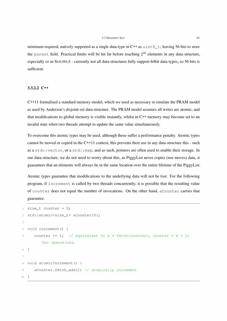
3.3 DISJOINT SET 61
minimum required, natively supported as a single data-type in C++ as uint8_t; leaving 56 bits to store
the parent field. Practical limits will be hit far before reaching 256 elements in any data-structure,
especially so in SOUFFLÉ - currently not all data-structures fully support 64bit data-types, so 56 bits is
sufficient.
3.3.2.2 C++
C++11 formalised a standard memory-model, which we used as necessary to emulate the PRAM model
as used by Anderson’s disjoint-set data-structure. The PRAM model assumes all writes are atomic, and
that modifications to global memory is visible instantly, whilst in C++ memory may become set to an
invalid state when two threads attempt to update the same value simultaneously.
To overcome this atomic types may be used, although these suffer a performance penalty. Atomic types
cannot be moved or copied in the C++11 context, this prevents their use in any data-structure this - such
as a std::vector, or a std::map, and as such, pointers are often used to enable their storage. In
our data-structure, we do not need to worry about this, as PiggyList never copies (nor moves) data, it
guarantees that an elements will always be in the same location over the entire lifetime of the PiggyList.
Atomic types guarantee that modifications to the underlying data will not be lost. For the following
program, if increment is called by two threads concurrently, it is possible that the resulting value
of counter does not equal the number of invocations. On the other hand, aCounter carries that
guarantee.
1 size_t counter = 0;
2 std::atomic<size_t> aCounter{0};
3
4 void increment() {
5 counter += 1; // equivalent to x = fetch(counter), counter = x + 1;
Two operations.
6 }
7
8 void atomicIncrement() {
9 aCounter.fetch_add(1) // atomically increment
10 }

3.3 DISJOINT SET 62
The memory ordering of atomics by default enforces sequential consistency, which dictates that for any
marked atomic operations, concurrent operations performed on them is equivalent to some sequential
ordering. We do not require the strong guarantee of sequential consistency - the strongest memory order
specified by the C++11 standard (Boehm and Adve, 2008) - instead we can relax to acquire and release
semantics. All these enforce are happens before and happens after ordering relationships for operations
on the same data. x86 architectures do not require special instructions for these acquire and release
orderings, as the architecture is designed with a strong ordering in mind. (McKenney, 2005)
The COMPARE-AND-SWAP operations have an equivalent primitive in C++11 , as a member function for
all atomic types. x.compare_exchange_strong(T& a, T b and x.compare_exchange_-
weak(T& a, T b) both atomically set x to b iff x = a, although the weak function is allowed to
fail spuriously.
The function signatures for the equivalent C++ disjoint-set operations are necessary to carry type defi-
nitions. As follows are the function declarations for FIND, UPDATE-ROOT, SAME-SET, UNION, and
NEW-ELEMENT. Note that makeNode() returns a packed value for the newly created singleton.
1 parent_t findElement(parent_t x);
2 bool updateRoot(const parent_t x,
3 const rank_t oldrank,
4 const parent_t y,
5 const rank_t newrank);
6 bool sameSet(parent_t x, parent_t y);
7 void unionNodes(parent_t x, parent_t y);
8 block_t makeNode();
3.3.3 PiggyList
Named due to the expanding nature of the data-structure, this is a new implementation and design of a
concurrent vector. As SOUFFLÉ deals with monotonically increasing data-structures (i.e. they are only
growing) except for clearing all elements, this allowed for a simpler, and more efficient data-structure.
Despite this, the data-structure can easily be modified to allow deletion, and also be lock-free. For
simplicity, the SOUFFLÉ implementation does not use these extensions.

3.3 DISJOINT SET 63
The requirements of the wait-free Union-Find implementation, is that on contention it retries, requiring
repeated find(u) calls that in turn necessitate random access to the storage container (i.e. access an
element at index i), in order to perform path compression. A std::vector is ill-suited to this task, as
concurrent writes or element creation that require expansion of the container capacity are not thread-safe.
A linked-list never changes the location of elements and as such can accommodate concurrent writes
and element creation; although the data-structure has poor random-lookup performance, but this can be
abated by increasing the number of elements stored in each node of the linked list. By storing say 10000,
elements within each node, the number of traversals required to be performed is cut down by a factor of
10000. Unfortunately, this is insufficient and still proves to be a bottleneck - using a larger number again
helps, although at a significant memory overhead for smaller lists. Figure 3.55 details what we will call
Blocklist, with chunk size k, also showing indexes 0, . . . , k + 2 containing elements.
FIGURE 3.55: Basic chunked-linked-list that has an access bottleneck
To address this shortcoming, the initial container size can be small (given as r), and future nodes in the
linked list use a size that is double the previous node’s size (i.e. 2r, then 4r, and so on), to which elements
can be inserted into. Starting with a container size of 1, the series of sizes per resize is 1, 3, 7, 15, ..., 2n−1.
Clearly, in a 64 bit system, no more than 64 nodes in our linked list will ever be required, which allows a
64 element long lookup-table, such that iteration is no-longer necessary.
Notably, this requires logarithms to identify which node a given index is, and would at first glance require
O(logn) time. Fortunately, the integer logarithm base 2 can be done in a constant number of CPU
cycles through the help of the gcc intrinsic __builtin_clzll (which counts the leading number
of bits, subtract this from 64 (for 8 byte unsigned integers) to get the index in the lookup-table), or if
not-compiling on gcc, the x86_64 instruction BSR performs the same operation.
For sections of SOUFFLÉ that are expected to always store a larger series of elements, a bigger initial
allocated block size can be used, as is in SOUFFLÉ , the default is an initial blocksize of 65535.
As previously mentioned, PiggyList does not move or copy any data. For the locking version, described
in Section 3.3.3.1, it is not required to keep around the old versions so as to allow copying over to the

3.3 DISJOINT SET 64
FIGURE 3.56: PiggyList with initial block size of 1; four elements have been created
new, larger container - strictly by design. This allows less memory overhead as compared to say, a
std::vector.
3.3.3.1 Implementation & Interface
The implementation of the basic PiggyList requires the use of locks. Note that the value modifications
are all performed atomically.
Algorithm 18 Appending an element to PiggyList
1: procedure APPEND(element)2: index← piggylist.size.fetch_add(1)3: if piggylist.container_size < index + 1 then . If this element’s location doesn’t exist4: piggylist.mutex.lock()5: while piggylist.container_size < index + 1 do . Double-checked lock6: . Allocate the next block into the lookup-table7: piggylist.blocks[piggylist.num_containers] = new block(2piggylist.num_containers)8: . The next allocated block will be twice as big9: piggylist.container_size += 2piggylist.num_containers
10: piggylist.num_containers++11: end while12: piggylist.mutex.unlock()13: end if14: . Set the element at its allocated index15: piggylist.blocks[blog2 index + 1c][index− (2blog2 index+1c − 1)] = element16: end procedure

3.3 DISJOINT SET 65
Algorithm 19 Retrieve an element in a PiggyList
1: procedure GET(index)2: return piggylist.blocks[blog2 index + 1c][index− (2blog2 index+1c − 1)]3: end procedure
As PiggyList has the concept of indexes, iteration is trivial. An iterator can be constructed with its
beginning at index 0, and terminating after index size− 1. A reverse iterator can be similarly constructed,
with its initial index at size− 1, terminating after reaching index 0.
3.3.3.2 Additional Features
Element deletion. As previously mentioned, PiggyList can be implemented to accommodate deletion.
In order to do so, a thread-safe linked list is also required, in order to store “deleted” elements’ indexes
(denoted in the following code as deleted_nodes). On element creation, if the linked-list is non-empty the
current thread will attempt to pop from the linked-list, and if successful, the element will be inserted at the
retrieved index, otherwise the element will be stored in the next available index (expanding if necessary).
Algorithm 20 Creating an element in a deletion enabled PiggyList
1: procedure APPEND(element)2: index← piggylist.deleted_nodes.pop()3: if index then . Check if there is a deleted element to re-use4: . Set the element at its allocated index5: piggylist.blocks[blog2 index + 1c][index− (2blog2 index+1c − 1)] = element6: else7: index← piggylist.size.fetch_add(1)8: if piggylist.container_size < index + 1 then . If this element’s location doesn’t exist9: piggylist.mutex.lock()
10: while piggylist.container_size < index + 1 do . Double-checked lock11: . Allocate the next block into the lookup-table12: piggylist.blocks[piggylist.num_containers] = new block(2piggylist.num_containers)13: . The next allocated block will be twice as big14: piggylist.container_size += 2piggylist.num_containers
15: piggylist.num_containers++16: end while17: piggylist.mutex.unlock()18: end if19: . Set the element at its allocated index20: piggylist.blocks[blog2 index + 1c][index− (2blog2 index+1c − 1)] = element21: end if22: end procedure

3.3 DISJOINT SET 66
To delete an element, the element can be destroyed at that index, and then the index is pushed onto the
linked-list.
Algorithm 21 Deleting an element
1: procedure REMOVE(index)2: cleanup element at index3: . signal that this index can be re-used4: piggylist.deleted_nodes.push(index)5: end procedure
The Figures 3.57, 3.58, 3.59, 3.60 show the resulting state during the sequence of deletions: delete(3),
delete(0), delete(4).
0 1 2 3 4 5 6 PiggyList:
Deletion Queue:
FIGURE 3.57: Starting PiggyList- occupied elements are labelled ingreen, unused in white
0 1 2 3 4 5 6 PiggyList:
Deletion Queue:
3
FIGURE 3.58: PiggyList after in-dex 3 has been deleted. Red is usedto mark deleted elements
0 1 2 3 4 5 6 PiggyList:
Deletion Queue:
3 0
FIGURE 3.59: PiggyList after in-dex 0 has been deleted
0 1 2 3 4 5 6 PiggyList:
Deletion Queue:
3 0 4
FIGURE 3.60: PiggyList after in-dex 4 has been deleted

3.3 DISJOINT SET 67
The next append operation will write into the first dequeued element from the front of the queue, in this
case writing into index 3.
In order to reclaim space, the following non-thread-safe procedure may be used - this runs in O(m+ n)
time, where m is the number of deleted elements, and n is the number of total elements in the data-
structure. If space reclaimation is not performed prior to iteration, it is necessary to insert tombstone or
markers for deleted elements, such that they can be skipped when reached.
Algorithm 22 Reclaiming space
1: procedure SHRINK(piggylist)2: final← index of the last element in the piggylist3: for each e ∈ deleted queue do4: . Only move elements towards the start of the list5: if e < final then6: move element at final into the index of e7: scan final back to point to the now-last element8: end if9: end for
10: remove blocks without elements11: end procedure
As follows is a pictorial representation of the trimming procedure, for the initial state as seen in Figure
3.61 which has elements at indices 1,4,5 already deleted.
0 1 2 3 4 5 6
4 1 5
final
FIGURE 3.61: Starting PiggyList- the final used index is 6
0 1 2 3 4 5 6
1 5
final
FIGURE 3.62: The element at in-dex 6 is moved to index 4, finaladvances to the last element (4)

3.3 DISJOINT SET 68
0 1 2 3 4 5 6
5
final
FIGURE 3.63: The element at in-dex 4 is moved to index 1, finaladvances to index 3
0 1 2 3 4 5 6
final
FIGURE 3.64: Index 5 is after thefinal index, so no elements aremoved. We terminate as there isno more elements in the deletionqueue
Wait-free. For a data-structure to carry the wait-free guarantee, each thread operating on the data-
structure must be able to finish in a finite number of steps, independent on the other threads’ operations.
PiggyList can carry this guarantee, albeit with concessions in its worst-case space complexity. This can
be abated by an extension, although this requires tuning to reduce contention as much as possible.
In order to be wait-free, the spin-locks that are used in container resizing must be replaced. When the
requested index is larger than the current container size, a compare-and-swap operation is performed on
the index of the lookup-table where the new segment would be placed. As follows is the pseudocode of
the makeNode() function.
Unfortunately, when many threads attempt to expand the container size at the same time, many container-
blocks will be allocated at the same time, which require deletion for the resulting failed threads. Worst-case
space complexity in this scenario is now O(nt), with t denoting the number of threads. Empirical data
of a small benchmark indicates this is not a rare occurrence, appearing to have a memory overhead of
approximately that of the worst case nt, as demonstrated in Figure 3.65. It is important to keep in mind
that instrumenting this memory usage undoubtedly increased the likelihood that a thread allocates memory
whilst another is currently in between allocating memory and attempting to mark it as authoritative. A
more accurate result may potentially be obtained by emulation, although this also carries complications.

3.3 DISJOINT SET 69
Algorithm 23 Creating an element in a wait-free PiggyList
1: procedure APPEND(piggylist, element)2: index← piggylist.size.fetch_add(1)3: block_index← blog2(index+1)c4: if piggylist.blocks[block_index ] is null then . Not allocated5: new_block← new block(2 block_index)6: . Try set allocated block if not already set7: if COMPARE-AND-SWAP(piggylist.blocks[block_index], null, new_block) = failure then8: clean up new_block9: end if
10: end if11: . Set the element at its allocated index12: piggylist.blocks[block_index][index− (2block_index − 1)] = element13: end procedure
0.0 0.2 0.4 0.6 0.8 1.0number inserted 1e9
0.0
0.2
0.4
0.6
0.8
num
bere
lem
ents
allo
cate
d
1e10
FIGURE 3.65: Memory consumption for a multithreaded insertion benchmark. Thenumber of threads in this test is 16.
In order to reduce the chances of this occurring, a weighted dice-throw is conducted per element-creation
that approaches 100% probability as the current container fills up. On a successful roll, the next container
size is allocated, still using the lock-free resizing algorithm. Note that the probability is weighted such
that it is not possible to allocate a new container that is not the current storing container’s successor -
i.e. if the current container is being added to, and a thread successfully rolls to create another container,
although the next one has already been reserved, that thread will not create it.
3.3 DISJOINT SET 70
Algorithm 24 Creating an element in a wait-free PiggyList
1: procedure APPEND(piggylist, element)2: index← piggylist.size.fetch_add(1)3: block_index← blog2(index+1)c4: if piggylist.blocks[block_index + 1] is null then . Next block free5: remaining← number of elements not occupied in this block6: if ROLL-DICE(remaining, 2block_index, t) then7: new_block← new block(2 block_index+1)8: . Try set allocated block if not already set9: if COMPARE-AND-SWAP(piggylist.blocks[block_index+1], null, new_block) = failure
then10: clean up new_block11: end if12: end if13: end if14: . Set the element at its allocated index, we assume current block is allocated15: piggylist.blocks[block_index][index− (2block_index − 1)] = element16: end procedure
The follwing dice roll predicate dice-roll provides a linear probability curve (visualised in Figure
3.66), in that as the current block fills up, the probability that a thread’s dice-roll will succeed also
increases. We coerce a guarantee that the threads must allocate if only t spaces are left in the container -
this ensures that all threads can assume that their current block_index will be writeable, as there is no
code-execution path for each thread that will allow no next block to be allocated, assuming t is known
ahead of time.
Algorithm 25 Dice roll predicate, if a thread should try to allocate a new block
1: procedure DICE-ROLL(remaining, blocksize, thread_count)2: . This ensures a thread’s index’s block always exists3: if remaining ≤ thread_count then4: return true5: end if6: return RAND([0, 1]) ≥ remaining
blocksize7: end procedure

3.3 DISJOINT SET 71
% occupied
probability
0 100%
1
0
t
FIGURE 3.66: Probability graph of the linear dice roll function, the last t threads areguaranteed to succeed
For the current dice-roll function, the probability of two nodes creating a new container at the same time
is dependent on many factors. For one, instructions may not necessarily take the same number of steps to
complete, and even the same instruction may be slower or faster depending on the calling context, the
scheduler, and other factors. If we try to assume that the threads will attempt to roll the dice at the same
time (which would seem to be a likely scenario for duplicate memory consumption), even if only one
thread succeeds, the thread may spend an arbitrary amount of time in the allocation block (i.e. within
the body of the roll-dice conditional), and so other threads may have ample opportunities to retry the
roll-dice functions on subsequent calls. Due to this, it is non-trivial to analyse complexity - even if it is
attempted, the number of assumptions may make it unrepresentative of real-world performance. Empirical
studies of probabilistic functions have proven sufficient in the literature of constructing concurrent data-
structures.(Gibson and Gramoli, 2015) It is worth noting that the worst-case space complexity is still
O(nt).
For this dice-roll predicate, the number of threads is known ahead of time as t. If for an application this is
not known, a modified probability function can ignore t, and instead in the append(e) function, an
additional check of the current block’s existence is necessary. For ease of space complexity evaluation,
the algorithm described in Algorithm 24 suffices.
An experiment into the space complexity of the probabilistic allocation approach using the linear
probability function defined above is presented in Figure 3.67. Spurious allocations of 2 or 3x are

3.3 DISJOINT SET 72
observed - a marked improvement over the ≈16x overhead of the non-probabilistic wait-free approach.
As we see in Section 3.3.4, this overhead is similar to that of a typical std::vector.
0.0 0.2 0.4 0.6 0.8 1.0number inserted 1e9
0.0
0.5
1.0
1.5
2.0
num
bere
lem
ents
allo
cate
d
1e9
FIGURE 3.67: Space consumption of a uniform probability Wait-free PiggyList
3.3.4 Disjoint Set and PiggyList Benchmarks
In order to measure the difference in utility of the different data-structures, a variety of scenarios will be
performed on the disjoint-set each using the different underlying data-structures. We only test the locking
versions without deletion, as the extensions are currently not required as part of the overall data-structure.
We measure the performance of the disjoint-set on several operations:
• Read heavy, minimal write (N − 1 consumers, 1 producer)
• Equal reading/writing (N/2 consumers, N/2 producers)
• Write heavy, minimal read (N − 1 producers, 1 consumer)
The following benchmarks were performed on a 8 Threaded machine with a Intel(R) Core(TM) i7-7700K
CPU @ 4.20GHz CPU.
Each thread operates on the same number of elements, disjoint from each other. In Snippet 3.8, the
consumer performs read-only tests whether elements are within the same disjoint set. This is read-only

3.3 DISJOINT SET 73
in the sense that the no path compression is performed, so no fields of the shared container are written
to. Snippet 3.9 shows the equivalence producer thread - it simply unions elements to be in the same set.
We union such that a large number of elements will be touched and have their fields updated. For the
consumer/producer tests, we run all of these over 8 threads.
LISTING 3.8: Consumer Pseudocode
1 void consume(size_t operations) {
2 for (size_t i = 1; i <
operations; ++i) {
3 disjointSet.readOnlySameSet(i,
i-1);
4 }
5 }
LISTING 3.9: Producer Pseudocode
1 void produce(size_t operations) {
2 for (size_t i = 0; i <
operations; ++i) {
3 disjointSet.unionNodes(i,
i/2);
4 }
5 }
We graph the total timings of the operations for an 8 threaded run (N=8).
Read heavy operations appear to scale better for PiggyList compared to the BlockList, beating the
runtime after around 2 million operations. The BlockList has block-size 10000 - if that is increased,
we observed that if this increases, the runtime only slightly improves. Looking at equal consumers and
producers shows that the BlockList scales much more poorly. The runtime of the std::vector is
magnitudes slower than either the BlockList or PiggyList. This trend is continued throughout rest of
these benchmarks.

3.3 DISJOINT SET 74
0 500 1000 1500 2000 2500 3000 3500 4000Number of elements (thousands)
100
101
102
Run
ning
Tim
e(m
s)Total Time:N-1 Consumers, 1 Producer
std::vectorBlockListPiggyList
FIGURE 3.68: Runtime for read heavy concurrent operations
As the number of writers increases the performance of the BlockList degrades drastically, while the
performance of PiggyList slightly decreases.

3.3 DISJOINT SET 75
0 500 1000 1500 2000 2500 3000 3500 4000Number of elements (thousands)
100
101
102
103
Run
ning
Tim
e(m
s)Total Time:N/2 Consumers, N/2 Producers
std::vectorBlockListPiggyList
FIGURE 3.69: Runtime for equal read/write heavy concurrent operations
For a large number of writers, the BlockList appears to perform better than the PiggyList, however after
around 1.3 million elements, the PiggyList supercedes.

3.3 DISJOINT SET 76
0 500 1000 1500 2000 2500 3000 3500 4000Number of elements (thousands)
100
101
102
103
Run
ning
Tim
e(m
s)Total Time:1 Consumer, N-1 Producers
std::vectorBlockListPiggyList
FIGURE 3.70: Runtime for write heavy concurrent operations
It is clear that the std::vector is vastly outclassed by the less-locking data-structures. In the following
graphs we breakdown the mean runtime for each producer and consumer, highlighting the consequential
interaction between different loads.
For the single producer benchmark, we see that the total runtime of the producing thread dominates
for PiggyList, whose performance only supersedes the equivalent BlockList producer after 2.3 million
elements. For the std::vector, both the producer and consumer threads have similar durations.

3.3 DISJOINT SET 77
0 500 1000 1500 2000 2500 3000 3500 4000Number of elements (thousands)
10−1
100
101
102
Run
ning
Tim
e(m
s)Time Breakdown:N-1 Consumers, 1 Producer
std::vector Consumerstd::vector ProducerBlockList ConsumerBlockList ProducerPiggyList ConsumerPiggyList Producer
FIGURE 3.71: Mean Producer/Consumer runtime for read heavy concurrent operations
As the number of producers increase, the BlockList consumer threads seriously degrade in performance,
consistently ranking slower than the producer thread. We see the similar reversing trend in PiggyList,
where the producers rank faster than the consumer threads.

3.3 DISJOINT SET 78
0 500 1000 1500 2000 2500 3000 3500 4000Number of elements (thousands)
10−1
100
101
102
103
Run
ning
Tim
e(m
s)Time Breakdown:N/2 Consumers, N/2 Producers
std::vector Consumerstd::vector ProducerBlockList ConsumerBlockList ProducerPiggyList ConsumerPiggyList Producer
FIGURE 3.72: Mean Producer/Consumer runtime for equal read/write heavy concurrent operations
For the maximum number of producers, we see that the performance of the two operations are almost
identical between all data-structures.

3.3 DISJOINT SET 79
0 500 1000 1500 2000 2500 3000 3500 4000Number of elements (thousands)
100
101
102
103
Run
ning
Tim
e(m
s)Time Breakdown:1 Consumer, N-1 Producers
std::vector Consumerstd::vector ProducerBlockList ConsumerBlockList ProducerPiggyList ConsumerPiggyList Producer
FIGURE 3.73: Mean Producer/Consumer runtime for write heavy concurrent operations
This demonstrates that the PiggyList has vastly better asymptotic complexity, however for small numbers
of operations, the BlockList mostly outperforms. We see this to not be the case for threaded element
creation - an often called operation during SOUFFLÉ operation.
In the following graphs we observe BlockList to consistently exhibit extremely poor performance for
all thread counts - it is outperformed by std::vector protected by a lock. Interestingly, we don’t
see a linear speed-up for PiggyList, even for large number of elements. We suspect this is due to the
highly contended atomic variable, which due to the x86 memory model, requires a relatively high level of
synchronisation between threads - even if requested to operate with a relaxed memory model as would be
possible with the PiggyList size variable.

3.3 DISJOINT SET 80
0 500 1000 1500 2000 2500 3000 3500 4000Number of elements (thousands)
101
102
103
Run
ning
Tim
e(m
s)
Total Time:Element Creation (1 thread)
std::vectorBlockListPiggyList
FIGURE 3.74: 1 Thread Insertion
0 500 1000 1500 2000 2500 3000 3500 4000Number of elements (thousands)
101
102
103
Run
ning
Tim
e(m
s)
Total Time:Element Creation (2 threads)
std::vectorBlockListPiggyList
FIGURE 3.75: 2 Threaded Parallel Insertion
0 500 1000 1500 2000 2500 3000 3500 4000Number of elements (thousands)
101
102
103
Run
ning
Tim
e(m
s)
Total Time:Element Creation (4 threads)
std::vectorBlockListPiggyList
FIGURE 3.76: 4 Threaded Parallel Insertion
0 500 1000 1500 2000 2500 3000 3500 4000Number of elements (thousands)
101
102
103
Run
ning
Tim
e(m
s)
Total Time:Element Creation (8 threads)
std::vectorBlockListPiggyList
FIGURE 3.77: 8 Threaded Parallel Thread In-sertion
The worst case memory consumption for the Locking PiggyList with deletion is the maximum number of
elements stored at once - even if the elements are removed one-by-one, as there is no de-allocation of
reserved blocks (unless shrinking is performed). As mentioned above, the wait-free PiggyList (with or

3.3 DISJOINT SET 81
without deletion) may use at most O(nt) space, in the scenario that all t threads attempt to allocate more
space, of which t− 1 threads later delete.
0.0 0.2 0.4 0.6 0.8 1.0Number of elements (billions)
0.0
0.2
0.4
0.6
0.8
1.0
1.2
1.4
1.6
Num
bero
fele
men
tsal
loca
ted
(bill
ions
)
Memory consumption of std::vector
FIGURE 3.78: Memory consumption of a std::vector as elements are inserted
It is interesting to compare the performance of the probabilistic wait-free PiggyList to a standard
std::vector. In Figure 3.78, we see similar memory overhead for the STL container, as compared to
the probabilistic wait-free PiggyList in practice in Figure 3.67. The locking PiggyList’s memory overhead
is tight, with no ‘spiked’-overhead when the container expands, shown in Figure 3.79. It is important to
note however, that this spiking is only consistently always observed within std::vector for when
non-trivially copyable objects are stored within the container. For trivially copyable types a realloc
will be attempted, so that if possible, the container is resized in-place, and no overhead will be seen (in
addition to not requiring copies of the objects stored). It is not simple to benchmark this, and it varies
wildly depending on the available RAM on the computer, the operating system, and the address space
variations induced by ASLR.

3.3 DISJOINT SET 82
0.0 0.2 0.4 0.6 0.8 1.0Number of elements (billions)
0.0
0.2
0.4
0.6
0.8
1.0N
umbe
rofe
lem
ents
allo
cate
d(b
illio
ns)
Memory consumption of PiggyList (locking version)
FIGURE 3.79: Memory consumption of a Locking PiggyList as elements are inserted
Single-threaded append performance: due to the lack of copying objects on resize, the PiggyList
will sometimes outperform a contiguous std::vector depending on the size of the data stored. In
the following benchmarks (Figures 3.80, 3.81, 3.82, 3.83) we measure the comparative performance of
std::vector::push_back and a modified PiggyList::append optimised for single-threaded
usage.

3.3 DISJOINT SET 83
0 10 20 30 40 50Number inserted (millions)
0
100
200
300
400
Tim
e(m
s)
PiggyListstd::vector
FIGURE 3.80: 8 bit (uint8_t)append performance
0 10 20 30 40 50Number inserted (millions)
0
100
200
300
400
Tim
e(m
s)
PiggyListstd::vector
FIGURE 3.81: 16 bit (uint16_-t) append performance
0 10 20 30 40 50Number inserted (millions)
0
100
200
300
400
Tim
e(m
s)
PiggyListstd::vector
FIGURE 3.82: 32 bit (uint32_-t) append performance
0 10 20 30 40 50Number inserted (millions)
0
100
200
300
400
Tim
e(m
s)
PiggyListstd::vector
FIGURE 3.83: 64 bit (uint64_-t) append performance
For 16 bit data-types and above, we observe an improvement in append performance. The benefit in 16
bits is marginal, for 32 bit a std::vector is just under 50% slower, and for 64 bit the std::vector
is just over half the speed of the PiggyList.
Whilst this tests only primitives, PiggyList also demonstrates improved performance for storing objects
that have costly move- or copy-constructors. PiggyList also has the benefit of being allowed to store non-
copyable or non-moveable types, such as std::atomic. In order to store these in a STL container, a

3.3 DISJOINT SET 84
pointer instead must be stored. This proves expensive as these would all require separate and independent
allocation, in addition to the allocation of new elements as the container expands. This is only applicable
to PiggyList implementations that do not perform node deletion, as supporting that requires movement or
copying of stored objects.

CHAPTER 4
Experiments
In order to demonstrate the use cases for native equivalence relations in Datalog, a series of experiments
have been set up. We compare the run-time of the implicit representation of equivalence relations to the
explicit representation in a real-world benchmark - identifying users from the Bitcoin blockchain. For
points-to analysis, we compare two different types of analyses, a subset based analysis and an equivalence
analysis - where the latter had not been able to be implemented in SOUFFLÉ until now due the associated
computational cost in a declarative programming language.
Datalog has only recently demonstrated productive examples of points-to analysis over billions of tuples,
as early as 2016. (Scholz et al., 2016) This was also performed in the SOUFFLÉ suite, on a similar input
domain as our points-to analysis performed in Section 4.2 on the OpenJDK. We demonstrate productive
examples of analyses generating a trillion tuples in under four seconds.
4.1 Bitcoin User Groups
Bitcoin provides a pseudonymous way of digital transactions, wherein transfers of the Bitcoin currency
are enabled through public transactions published on the blockchain. Figure 4.1 provides a simplified
view of how each published block (occurring approximately every 10 minutes) contains a series of
transactions, a hash of the previous block and additional data.
85

4.1 BITCOIN USER GROUPS 86
Prev Hash Nonce
Block
Tx Tx Tx ... Tx
Prev Hash Nonce
Block
Tx Tx Tx ... Tx
Prev Hash Nonce
Block
Tx Tx Tx ... Tx
Newer Blocks
FIGURE 4.1: The blockchain structure (Modified from (Nakamoto, 2008))
For our purposes, we consider each transaction to contain a series of input identifiers which are the public
keys corresponding to the private keys used to sign the transaction, a series of output identifiers which are
the public keys of the receiving users and the quantity of Bitcoin to send them each, and finally a hash of
the entire transaction. We picture a simplified transaction in Figure 4.2.
Addresses In: 1AHBN8YuQVqKLzZo4V2L5WCxewwr7xtDHS 1HvhZyxtJfSWxDJjcpM8THfQ3yB6GPxZX9
Addresses Out:
1Lq5DVmok8p9opyy5QFBX2cM48xTELecaj 16ZdsGm3J9uTt5K7N8ojW8D66X7kMJCytS
Transaction Hash c1c50ac324f45d0ecc2d8b1708666ca43ea894ebaf9cb79aceba914867c029c5
FIGURE 4.2: A simplified Bitcoin transaction
The public keys have an associated private key, which must be used in order to ensure authenticity
of that action via the act of signing - similar to how an ordinary cheque requires the signature of the
sender in order to be valid. This private key must be secret, otherwise an adversary will be able to
create transactions on behalf of the private key owner. A demonstration of the signing, and associated
verification is pictured in Figure 4.3. The public key is considered public, that is, anyone is able to possess
it without consequence - and in fact is required to if they wish to confirm the validity of the transaction. A
new private-public key pair is typically generated per transaction, as this is considered good practice for a
payee. (Reid and Harrigan, 2013) The word wallet is often used to describe addresses that have Bitcoin
amounts associated with them, analogous to a wallet that contains cash. After the transaction is signed, it

4.1 BITCOIN USER GROUPS 87
is forwarded on to the Bitcoin network to be added into the next available block (provided it has provided
a large enough transaction free & the transaction is valid).
Pay $500 to Charlie
Alice's public key
Sign
6EB69570 08E03CE4
Verify
Alice's private key
Alice
Bob
Pay $500 to Charlie
FIGURE 4.3: Signing a transaction with a private key (Modified from (GÃuthberg, 2006))
As the private key must be secret, we are able to consider all transactions associated with the corresponding
public key to have been created by the same user. For any meaningful analysis over the user distribution, it
is necessary to group public keys by the user that owns them. Reid and Harrigan proposed considering all
public keys that are input to the same transaction to be controlled by a single person, as they require control
of the associated private keys. (Reid and Harrigan, 2013) The website WalletExplorer (Janda, 2013)
uses this heuristic in order to identify Bitcoin exchanges (sites that are used to trade fiat currencies with
cryptocurrencies like Bitcoin). (jstolfi , https://www.reddit.com/user/jstolfi) As noted, this is inaccurate
due to some Bitcoin services handling private keys and mix inputs together as part of their methodology.
Notably, this heuristic can be represented by an equivalence relation, as it is reflexive (public keys are
owned by the same user as their own user), symmetric (likewise), and transitive (inputs across multiple
transactions may be shared). We wish to demonstrate the efficiency of the implicit representation over the
previous method of explicit representation of equivalence relations.

4.1 BITCOIN USER GROUPS 88
4.1.1 Input Dataset
As our dataset, we use a subset of all Bitcoin transactions from 2017 - there are over 200 million
transaction/input pairs that year. We are only able to analyse a subset of the transactions due to the
computational and space requirements of doing so. In Table 4.1, the left-hand column denotes how many
pairs are loaded in as facts. This data was scraped using the high-performance BlockSci tool (Kalodner
et al., 2017), which enables simple interaction with the large blockchain dataset, and provides a multi-
threaded method to extract data.
Size PubKeys Transactions Classes Singletons Largest Class Mean Size Same User Pairs1000 971 935 906 854 5 1.07 11355000 4685 4117 3803 3303 11 1.23 794710000 9141 7516 6662 5726 42 1.37 2696550000 40893 29881 24451 21929 1420 1.67 3764247100000 76129 54555 43335 38185 2768 1.76 13351193500000 343008 236291 171874 144299 9675 2.00 2862929181000000 717098 481599 340467 279324 29344 2.11 14651938965000000 3442156 2737910 1776519 1469558 61384 1.94 1209691188810000000 6631620 5461708 3411035 2834282 124007 1.94 49007650539
TABLE 4.1: Statistics of the input data set
Whilst large-scale Datalog analyses have been performed, these examples did not contain examples of
transitivity which is what we believe to be the largest contributor of program execution time in our run of
the explicit representation, as described earlier in Section 2.3.
4.1.2 Datalog Programs
To demonstrate the conciseness of implementing this experiment, Snippet 4.1 is the Datalog program
used for the implicit equivalence relation. We mark the same_user(user1, user2) relation as an
equivalence relation (eqrel) to induce the reflexive, symmetric, and transitive nature of this relationship
between transactions. We make modifications to the generated C++ file in order to benchmark the
individual components of the runtime: I/O, solving, and enumeration over all pairs. For the enumeration
over all pairs, it was necessary to omit writing the output and instead increment an atomic integer, in
order to focus entirely on the speed of iteration, thus removing the bottleneck of disk I/O. It was not
necessary to speed up for input (perhaps via mapping the fact file into a RAM disk), as these facts from
the extensional database (EDB) were loaded into a regular relation, identical between both implicit and

4.1 BITCOIN USER GROUPS 89
explicit equivalence relation programs - and thus do not interfere with the experiment as we discard these
index timing from the total compared solving time.
Iteration over the final output pairs (in this case, the pairs of users that are classified as the same) is done
in a single thread, as it typically is written to disk. We modify this to occur in parallel through augmenting
the generated C++ file, to simulate the rule being fed into another rule. This allows us to compare the
iteration speeds over the relation across implementations.
These experiments were each run 5 times each, and averaged out except for those exceeding computational
time or crashing, as marked.
LISTING 4.1: Implicit Equivalence Relation Benchmark Program
1 .type TxId
2 .type PubKey
3 .decl transaction_input(tx : TxId, userIn : PubKey)
4 .input transaction_input()
5 // whether two users are the same
6 .decl same_user(user1 : PubKey, user2 : PubKey) eqrel
7 .output same_user()
8
9 same_user(u1, u2) :-
10 transaction_input(tx, u1),
11 transaction_input(tx, u2).
The comparative explicit implementation requires an additional two rules for symmetry and transitivity to
form an equivalence relation - reflexivity is not required, as within the same_user_explicit(u1,
u2) rule on line 9, there is no restriction that u1 and u2 must be different.
LISTING 4.2: Explicit Equivalence Relation Benchmark Program
1 .type TxId
2 .type PubKey
3 .decl transaction_input(tx : TxId, userIn : PubKey)
4 .input transaction_input()
5 // whether two users are the same
6 .decl same_user_explicit(user1 : PubKey, user2 : PubKey)

4.1 BITCOIN USER GROUPS 90
7 .output same_user()
8
9 same_user_explicit(u1, u2) :-
10 transaction_input(tx, u1),
11 transaction_input(tx, u2).
12 // symmetry
13 same_user_explicit(u1, u2) :- same_user_explicit(u2, u1).
14 // transitivity
15 same_user_explicit(u1, u3) :- same_user_explicit(u1, u2),
same_user_explicit(u2, u3).
4.1.3 Results
This experiment also demonstrates the current cost of reading in facts, in Figure 4.4 we demonstrate
the cost of loading in these input tuples from disk, as well as the associated memory of the program up
until that point. We observe a rough proportional relationship between fact read in time and memory
consumption of the loaded facts, consistent with the internal storage implementation of SOUFFLÉ . We
use the GNU time program (version 1.7) to measure this, using the -f "%e" flag, which prints the
peak RSS in kilobytes, (Eddelbuettel, 2000) and terminating the program after all the threads have been
read from file.

4.1 BITCOIN USER GROUPS 91
1 5 10 50 100 500 1000 5000 10000Number of Bitcoin Transactions (thousands)
10−3
10−2
10−1
100
101Ti
me
(s)
I/O Time and Memory Consumption
Time (s)Memory (MB)
101
102
103
Mem
ory
(MB
)
FIGURE 4.4: Memory and time consumption of the input symbol table
SOUFFLÉ transforms input terms from symbols to numbers within the RamDomain, that is, any term of a
fact is mapped to an integer, similar to the densification step in our data-structure. Whilst this does mean
that the arguments inserted into the equivalence relation data-structure are assigned ordinal numbers twice,
this is necessary as if other facts or symbols are read in from file (or in fact generated via concatentation
and aggregations in Datalog) before, the arguments inserted into the equivalence relation are no longer
the sequential numbers starting from 0. On top of this, numeric types (.type number) do not have
mapping applied to them, so inserting these into the equivalence relation requires densification in order to
ensure a low footprint.
This mapping from symbol to numbers is not well optimised - it uses a std::unordered_map on
a single thread, with all files loaded in sequentially. A future improvement to SOUFFLÉ may include
optimising this to perform I/O in parallel when possible. Internal code profiling showed that the hash-map
was the bottleneck compared to disk read time, and thus could be replaced with a concurrent equivalent,
wherein a busy-queue can insert into, where the queue is populated from the fact files.
Figure 4.5 (log scale) demonstrates the solving time for the same_user predicate, which excludes
reading facts from file, and iterating over the final derived facts.

4.1 BITCOIN USER GROUPS 92
1000 5000 10000 50000 100000 500000Number of Input Tuples
10−3
10−2
10−1
100
101
102
103
104
105
Tim
e(s
)
Solving Time
Eqrel: 1 threadEqrel: 2 threadEqrel: 4 threadEqrel: 8 threadExplicit: 1 threadExplicit: 2 threadExplicit: 4 threadExplicit: 8 thread
FIGURE 4.5: Solving time for the same_user* predicate for the Bitcoin data set
Input SizeEqrel Explicit
Threads1 2 4 8 1 2 4 8
1000 0.00062 0.00062 0.00081 0.0038 0.0015 0.0014 0.0013 0.00175000 0.0036 0.0030 0.0025 0.0054 0.013 0.011 0.01 0.01410000 0.0078 0.0060 0.0046 0.0066 0.048 0.036 0.029 0.03250000 0.087 0.053 0.032 0.027 72 36 18 15100000 0.29 0.17 0.093 0.070 490 240 120 100500000 4.7 2.6 1.4 0.99 51000* 21000* 11000* 8600*1000000 10 5.6 2.9 2.1 - - - -5000000 46 25 13 9.4 - - - -10000000 93 51 26 19 - - - -
TABLE 4.2: Solving Time (seconds, 2 s.f.), * indicates the experiments were only ran once
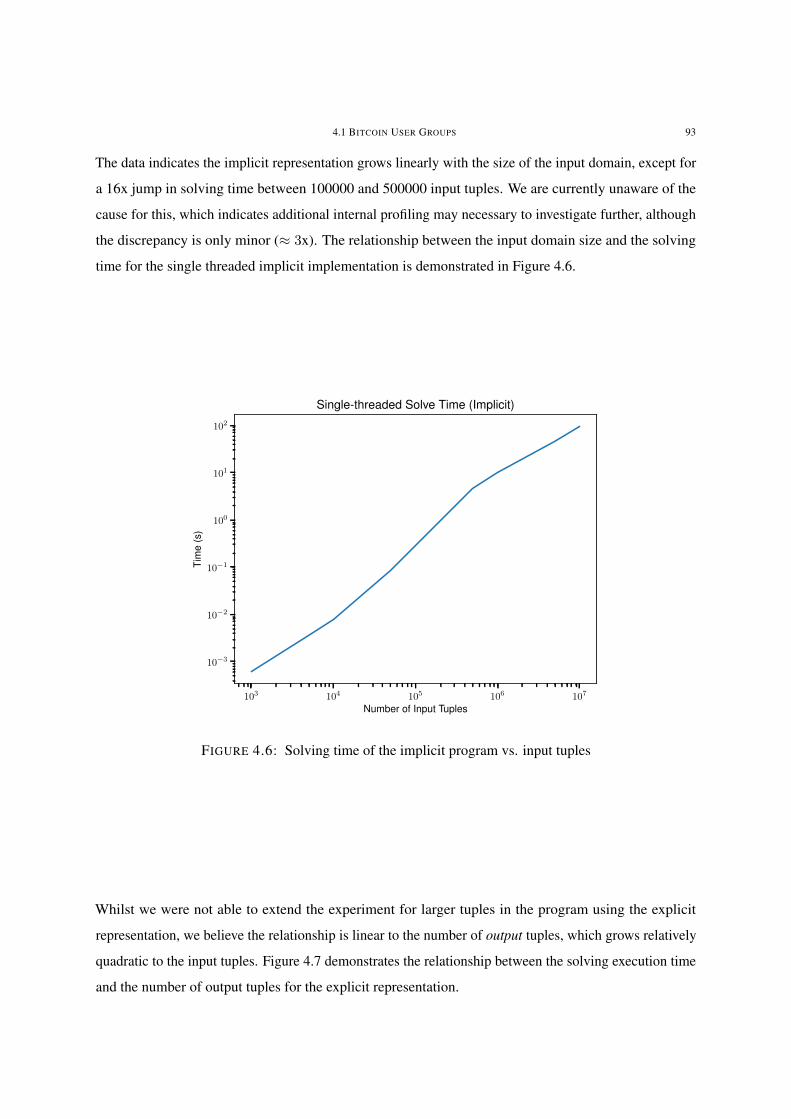
4.1 BITCOIN USER GROUPS 93
The data indicates the implicit representation grows linearly with the size of the input domain, except for
a 16x jump in solving time between 100000 and 500000 input tuples. We are currently unaware of the
cause for this, which indicates additional internal profiling may necessary to investigate further, although
the discrepancy is only minor (≈ 3x). The relationship between the input domain size and the solving
time for the single threaded implicit implementation is demonstrated in Figure 4.6.
103 104 105 106 107
Number of Input Tuples
10−3
10−2
10−1
100
101
102
Tim
e(s
)
Single-threaded Solve Time (Implicit)
FIGURE 4.6: Solving time of the implicit program vs. input tuples
Whilst we were not able to extend the experiment for larger tuples in the program using the explicit
representation, we believe the relationship is linear to the number of output tuples, which grows relatively
quadratic to the input tuples. Figure 4.7 demonstrates the relationship between the solving execution time
and the number of output tuples for the explicit representation.

4.1 BITCOIN USER GROUPS 94
103 104 105 106 107 108
Number of Output Tuples
10−3
10−2
10−1
100
101
102
103
104
105
Tim
e(s
)
Single-threaded Solve Time (Explicit)
FIGURE 4.7: Solving time of the explicit program vs. output tuples
In addition to the poor running time, the number of generated tuples for the explicit version is inconsistent
with both the implicit implementation and a custom imperative implementation of the program. This oc-
curs for all numbers of threads, indicating that it is not a race condition, but instead an issue with handling
large programs. Interestingly the single threaded explicit program was the most inaccurate, generating
319687058 output pairs compared to the correct amount of 286292918, a 12% over-approximation. The
2, 4, and 8 threaded programs each generated incorrect numbers of output tuples, albeit within a 1% error
margin.
We also observed the eqrel (implicit) programs for 10 million input tuples crashing occasionally, either
due to exceptions or segmentation faults. 1 out of 5 of the single threaded runs segfaulted, no two-threaded
runs crashed, 1 of the 5 four-threaded runs caused an exception, and 2 of 5 runs of the eight-threaded run
segfaulted. We are currently unaware of the cause of this behaviour.
Iteration time over the pairs indicates an overhead for the smaller sized equivalence relations in the
implicit representation, gradually matching the performance as the number of output tuples increases.
This overhead is most apparent for operation over 1000 to 10000 input tuples inclusive, which we attribute
to the constant time overhead of managing a hash-map and lists in generating the equivalence cache in the
implicit representation program. Figure 4.8 demonstrates the timings against the number of input tuples.

4.1 BITCOIN USER GROUPS 95
Note that the iteration is for an incorrect number of tuples for the 500000 input tuple explicit program,
which potentially provides a 12% slowdown for the explicit single-threaded program.
11357947
26965
3764247
13351193
286292918
Number of Output Tuples
10−3
10−2
10−1
100
101
Tim
e(s
)
Iteration Time
Eqrel: 1 threadEqrel: 2 threadEqrel: 4 threadEqrel: 8 threadExplicit: 1 threadExplicit: 2 threadExplicit: 4 threadExplicit: 8 thread
FIGURE 4.8: Iteration time versus the number of output tuples
It is interesting to note that the iteration time of the single-threaded implementation is consistently
equal or better than the parallel iteration, despite it being intuitive that the threads are performing work
independently. We are currently unsure of where this discrepancy lies, as it exists in both eqrel and
explicit programs which may indicate a internal SOUFFLÉ issue. Internal profiling may be required to
resolve the root cause. This time may also not be indicative to the actual iteration time over the pairs, as
we increment an atomic integer to count the number of output tuples, as well as preventing the loop from
being optimised out. In fact, this atomic integer may be the cause for the slowdown over multiple threads,

4.1 BITCOIN USER GROUPS 96
as despite our usage of the relaxed memory consistency model for this variable, the x86 architecture
has strong memory guarantees as a baseline standard (Preshing, 2012) so contention over this variable
may cause excessive synchronisation, and thus a slowdown in execution. If this is the case, it would also
explain performance discrepancies with the performance of increasing parallelism with PiggyList.
For profiling the memory consumption, we measure the peak RSS (resident set size) memory usage,
which incidentally also includes the I/O symbol table. Figure 4.9 demonstrates the increase in the memory
consumption of programs, with Table 4.3 detailing the figures.
103 104 105 106 107
Number of Input Tuples
101
102
103
104
Mem
ory
(MB
)
Memory Consumption - Single Threaded
EqrelExplicit
FIGURE 4.9: Memory use for both representations versus the number of input tuples
Input Size Memory Consumption (MB)Implicit Explicit
1000 6.9 6.45000 15 1510000 23 2650000 73 270100000 130 790500000 560 130001000000 1100 -5000000 5400 -10000000 11000 -
TABLE 4.3: Memory Consumption of the Bitcoin Benchmarking Programs (MB, 2 s.f.)

4.2 STEENSGAARD ANALYSIS 97
Based on the figures, we observe a roughly linear increase in the memory consumption for the implicit
representation, whereas for the explicit representation the growth appears roughly quadratic.
4.1.4 Discussion
We observe a near-quadratic runtime for the explicit representation, while the implicit representation was
approximately linear, as was expected. This demonstrates that on real-world data-sets, even for those with
medium-sized equivalence classes, quadratic run-times for the explicit representation will be observed,
and thus using the implicit representation will dramatically improve solving performance for programs
containing equivalence relations.
This trend was also observed for space consumption - we demonstrate that an explicit representation does
in fact take quadratic space to represent, as was difficult to show in Section 3.1.5 as the time complexity
of the explicit representation made benchmarks impractical.
A simple single-threaded Python imperative implementation took around 41 seconds to perform Union-
Find over the 10 million input domain. The declarative implementation is only slower by a factor of 2, a
narrower gap than usual - typical declarative programs are often magnitudes slower than their imperative
equivalents. (Kastrinis et al., 2018) SOUFFLÉ was originally designed to provide similar performance to
imperative implementations, and to be simpler to write. (Scholz et al., 2016)
4.2 Steensgaard Analysis
In order to statically analyse a program, the notion of memory modelling must be explored. One form of
modelling is points-to analysis, which computes the objects that variables can point to over the duration of
the program. As the amount of memory that will be allocated during a program could be unbounded (as
is the case in Snippet 4.3), we require a memory abstraction. We treat all objects allocated at a program
site to be interchangeable, and represent them by a single symbol. This method is known as representing
each dynamic heap object their abstract location. (Sridharan et al., 2005) In Snippet 4.3, we may say the
variable x points to o4, where oi refers to the object allocated on line i.
LISTING 4.3: Unknown quantity of memory allocation
1 int* foo() {
2 int* x;

4.2 STEENSGAARD ANALYSIS 98
3
4 while(condition) x = (int*) malloc(sizeof int);
5
6 return x;
7 }
This form of memory modelling was introduced by Andersen, (Andersen, 1994) where interactions
between variables can be modelled via subset-constraints on their respective points-to sets. If a variable
has the assignment y = z, then we say that the points-to set of y presumes all points-to elements of
z - that is, pts(y) ⊇ pts(z), where pts(y) denotes the points-to set of y. This form of analysis was
initially performed as flow-insensitive and context-insensitive meaning that the flow (or ordering of
executed statements) of the program nor the execution contexts (i.e. where/what called the functions)
are considered. This analysis carries a worst case cubic complexity (Shapiro and Horwitz, 1997); a
less accurate, but significantly faster analysis was proposed by Steensgaard that ran in O(αn) time,
using union-find data-structures. (Steensgaard, 1996) This analysis carries the same flow- and context-
insensitivity and Andersen’s original analysis. The Steensgaard is much less accurate for a points-to
analysis as it merges points-to sets on assignment, rather than retaining it as a subset constraint. This has
the benefit of being trivially representable within a union-find data-structure (objects that share the same
points-to set are within the same set within a disjoint-set structure), however will result in extremely large
overheads.
Adding either flow- or context-sensitivity to a points-to analysis increases the usefulness of the points-to
analysis, (Lhoták and Hendren, 2006) however the computational cost of such an analysis dramatically
increases, although specialised methods exist to compute these. (Whaley and Lam, 2004)
4.2.1 Field-Sensitive Analysis
In addition to these, a field-sensitive analysis allows writes and reads to fields within records or objects to
be disambiguated from other fields. Bodik & Sridharan proposed a simple flow-sensitive analysis, (Srid-
haran et al., 2005) that performs conditional points-to - if a variable a loads from a field b1.f, whilst a
variable c stores to field b2.f, then a may point-to the same objects that c points to, if b1 and b2 point
to shared memory. When two variables are said to point-to the same memory (i.e. the intersection of their
points-to sets is non-empty), they are said to alias.

4.2 STEENSGAARD ANALYSIS 99
In Table 4.4, we construct the Bodik field-sensitive analysis, in addition to a modified Steensgaard
analysis, which adds conditional assignment over aliasing fields.
Description Assignment ConstraintBodik Steensgaard*
Allocation a = new o() o ∈ pts(a) o ∈ pts(a)Assignment a = b pts(a) ⊇ pts(b) pts(a) = pts(b)
Conditional Alias a = b1.f; b2.f = calias(b1, b2)⇒pts(a) ⊇ pts(c)
alias(b1, b2)⇒pts(a) = pts(c)
TABLE 4.4: Constraint rules for the simplified field-sensitive language grammar
For the following program in Snippet 4.4, the corresponding to field-sensitive points-to set is depicted in
Figure 4.10. For this example, both Bodik and Steensgaard* analyses result in the same points-to set. On
line 5, the variable z is stored to y.f, whilst on line 6 the variable w.f is loaded from into v. As y and
w alias (they both point to at least one shared object), the conditional alias holds, and thus we perform the
equivalent operation for v = z. For our simplified Steensgaard analysis, we merge the two points-to
sets of z and v, whilst for Bodik, we apply a subset constraint.
1 x = new o(); // o12 z = new o(); // o23 w = x;4 y = x;5 y.f = z;6 v = w.f;
LISTING 4.4: Examplefield-sensitive program (Sridharanet al., 2005)
x
y
w
O 1
v
z O 2
FIGURE 4.10: Resulting points-toset - field sensitive analysis
These Steensgaard analyses have typically had difficulty in matching the expected near-linear time when
applied in a declarative context. Steensgaard relies on disjoint-sets which is by, implementing union-find,
a destructive data-structure and thus is difficult to directly represent purely declaratively. Very recently,
there have been promising results from expressing the union-find data-structure as purely declarative
statements within the LogicBlox Engine. (Balatsouras et al., 2017) We wish to explore this in future

4.2 STEENSGAARD ANALYSIS 100
work.The equivalence relation that is induced by the use of the equality-based set operations can be
simulated by the three explicit rules for reflexivity, symmetry, and transitivity, at the expense of efficiency.
However, for this input size it is not feasible to compute the Steensgaard analysis with the explicit
representation. As the explicit representation run-time is proportional to the total number of output tuples
stored (observed in Section 4.1), and the output tuples for the Steensgaard program is a trillion, a rough
back of the envelope calculation shows it would take over 6 years to calculate (14 hours for the 280
million tuple program⇒ 14 hours× 1151866748812286292918 ≈ 6.6 years).
4.2.2 Datalog Programs
We perform this benchmark using for two programs; a field-sensitive Steensgaard analysis written using
the implicit equivalence relations (Snippet 4.6), and a field-sensitive Bodik analysis written with subset
constraints (Snippet 4.7). All files share the same header, which declares the input rules (Snippet 4.5).
LISTING 4.5: Common Input Rules
1 // o: x := new T()
2 .decl alloc(x:symbol, o:symbol)
3 // x := y;
4 .decl assign(x:symbol, y:symbol)
5 // x := y.f;
6 .decl load(x:symbol, y:symbol, f:symbol)
7 // x.f := y;
8 .decl store(x:symbol, f:symbol, y:symbol)
9
10 // input EDB as CSV files
11 .input alloc, assign, load, store
Instead of iterating over all the derived tuples (as they vary massively in size between analyses), we
simply print the size of the relation, which is the number of tuples stored. We mark the var points-to set
(vpt) as eqrel to act an equivalence relation and thus represent tuples implicitly.
LISTING 4.6: Steensgaard Field-Sensitive Analysis in SOUFFLÉ
1 .decl vpt(x:symbol, y:symbol) eqrel
2 // allocation sites
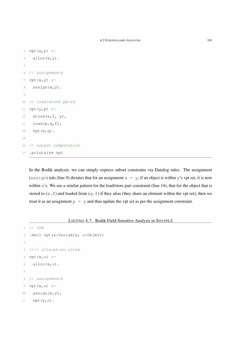
4.2 STEENSGAARD ANALYSIS 101
3 vpt(x,y) :-
4 alloc(x,y).
5
6 // assignments
7 vpt(x,y) :-
8 assign(x,y).
9
10 // load/store pairs
11 vpt(y,p) :-
12 store(x,f, y),
13 load(p,q,f),
14 vpt(x,q).
15
16 // output computation
17 .printsize vpt
In the Bodik analysis, we can simply express subset constrains via Datalog rules. The assignment
(assign) rule (line 9) dictates that for an assignment x = y, if an object is within y’s vpt set, it is now
within x’s. We see a similar pattern for the load/store pair constraint (line 14), that for the object that is
stored to (x.f) and loaded from (q.f) if they alias (they share an element within the vpt set), then we
treat it as an assignment p = y and thus update the vpt set as per the assignment constraint.
LISTING 4.7: Bodik Field-Sensitive Analysis in SOUFFLÉ
1 // IDB
2 .decl vpt(x:Variable, o:Object)
3
4 //// allocation sites
5 vpt(x,o) :-
6 alloc(x,o).
7
8 // assignments
9 vpt(x,o) :-
10 assign(x,y),
11 vpt(y,o).

4.2 STEENSGAARD ANALYSIS 102
12
13 // load/store pairs
14 vpt(p,o2) :-
15 store(x,f, y), // x.f := y
16 load(p,q,f), // p := q.f
17 vpt(x,o1), // alias x q
18 vpt(q,o1),
19 vpt(y,o2).
20
21 // output computation
22 .printsize vpt
4.2.3 Results
Loading in the facts from file consistently takes ≈ 5 seconds, and 992MB of memory. This consists
of four fact files: alloc.facts (58MB), assign.facts (275MB), load.facts (31MB), and
store.facts (9.8MB). This is the same for both Steensgaard and Bodik analyses. Running the two
results in vastly different points-to sets - as Steensgaard is an over-approximation of the points-to set as
compared to Bodik. The final count for Steensgaard is 1151866748812 (1.1 trillion) tuples, whilst for
Bodik 389210 output tuples are generated. We believe this is the first Datalog program to have stored a
trillion tuples, as Steensgaard analyses heavily favour imperative implementations and thus have not seen
implementation in declarative languages before.
The solving runtime for the analyses is demonstrated in Figure 4.11 and Table 4.5.

4.2 STEENSGAARD ANALYSIS 103
1 2 4 8Threads
0
1
2
3
4
5
Tim
e(s
)
Points-to Analysis Solve-time
SteensgaardAndersen
FIGURE 4.11: Solving time for various thread counts for each analysis
Threads AnalysisSteensgaard Bodik
1 5.6 5.22 4.5 3.14 3.6 2.18 3.3 1.5
TABLE 4.5: Solving time for the points-to analyses (seconds, 2 s.f.)
We can see that the Steensgaard analysis takes longer to solve than the Bodik analysis, and that the gains
from adding additional threads does not significantly improve the running time as compared to the Bodik
analysis. We can partition the solving program into several stages for each analysis, as is observed within
the generated C++ code:
Steensgaard:
(1) alloc - insert all rules from the alloc relation
(2) assign - insert all rules from the assign relation
(3) extend - insert knowledge learned from the delta into the current knowledge

4.2 STEENSGAARD ANALYSIS 104
(4) insert all - used to generate a delta relation for the next step
(5) load store - perform the semi-naïve evaluation on this relation until fixed-point
From manual analysis of the generated C++ code, we see that the extend is unnecessarily inserted in
this case, as no information has been loaded into the relation as used passed into the extend operation.
Omitting this reduces the run-time, but may not necessarily be done automatically, as it depends on the
program loaded in and thus may introduce incorrect behaviour if applied generally.
Bodik:
(1) alloc - insert all rules from the alloc relation
(2) insert all - used to generate a delta relation for the next step
(3) mixed (assign & load store) - perform the semi-naïve evaluation until fixed-point
As the assign and load/store rules are both recursive, these are performed in the same loop, until
a fixed-point is reached, as new knowledge in one may generate knowledge in the other rule.
Due to this structural difference in the resulting program, we present the time breakdown for the above
sections in Table 4.6.
Threads Steensgaard Bodikalloc assign extend insert all load store alloc insert all mixed
1 0.34 1.4 1.0 2.0 0.81 0.23 0.19 4.72 0.27 0.94 0.78 1.8 0.67 0.15 0.16 2.84 0.20 0.61 0.58 1.8 0.44 0.13 0.23 1.88 0.18 0.45 0.52 1.8 0.37 0.13 0.19 1.2
TABLE 4.6: Time breakdown of the points-to analysis
As mentioned, by removing the unnecessary extend section of the generated code, we are able to save
up to a second. The portion of generated code that takes the longest time is the insert all snippet.
This also demonstrates a poor threaded scaling - this is due to it not being implemented via OpenMP. It is
possible to do so, but was omitted based on incorrect assumptions (as this demonstrates). It would be
beneficial to repeat this benchmark again with this changed. These changes would bring the Steensgaard
implementation to only have a marginal overhead over the Bodik analysis.

4.2 STEENSGAARD ANALYSIS 105
As demonstrated in Figure 4.12, the memory overhead for the Steensgaard analysis is comparable to the
computational overhead.
Steensgaard AndersenAnalysis
0
200
400
600
800
1000
1200
1400
Mem
ory
(MB
)
Points-to Analysis Memory Consumption
FIGURE 4.12: Maximum resident memory size for each analysis
We believe the potential changes made above would not have an effect in the overall memory consumption.
4.2.4 Discussion
Steensgaard analysis was proposed to combat the associated cost of Bodik analysis, (Steensgaard,
1996) due to the poor computational power at the time of their introduction in the 1990s. Since then
computational power has dramatically improved, and as such, the runtime of an Bodik analysis (worst-case
cubic) is negligible on modern hardware.
However, despite the recent rise of declarative languages for performing of points-to analysis, Steensgaard
analyses were still strictly confined to imperative implementations due to their nature. (Kastrinis et al.,
2018) In demonstrating similar performance we believe we have proven that Steensgaard analyses are
now reasonable within Datalog.

4.2 STEENSGAARD ANALYSIS 106
There are multiple optimisations that could be made, based on the above performance analysis, with
the performance breakdown indicating that the lack of parallelism for some operations significantly
contribute to the running time for larger programs.
CHAPTER 5
Future Work
Based on both the internal micro-benchmarks (i.e. benchmarking the individual layers) and the full
system benchmarks showed areas of improvement. These may potentially be both in the algorithms for
each operation, or, within the choice of data-structures and potential micro-optimisations. As the program
is highly repetitive in that some functions are called millions, billions, or even trillions of times, minor
improvements in code may correspond to significant improvements in memory usage or runtimes.
As noted in the related work, a recent paper An Efficient Data Structure for Must-Alias Analysis by
Kastrinis et al. investigates the use of a declarative union-find program for a points-to analysis - that is,
union-find was implemented via pure Datalog statements. Writing equivalent SOUFFLÉ programs and
comparing the runtime to our implicit implementation is a highly relevant area of further research. We
were not able to perform this due to the implicated time constraints with such a recently published paper.
We note further areas of research and improvement that could be made in the various layers of the
data-structure.
5.1 Equivalence Relation
Currently, users of SOUFFLÉ must must tag their relations as eqrel in the declaration in order to generate
the implicit behaviour. It is possible to perform an analysis on the relations to detect equivalence relations
automatically via detecting reflexive, symmetric, and transitive rules. Pattern matching is one way to
achieve this, however this may not capture all equivalence relations. This behaviour may be unwanted,
as some SOUFFLÉ features were not designed for use with implicit relations as this implementation is
the first example of such functionality. This interfered with separate features such as provenance (i.e.
computing which rules were used to compute a fact), and magic-set optimisations - discussion with the
107

5.2 SPARSE MAPPING 108
other developers of SOUFFLÉ indicates this is primarily due to problems in the implementation of, and
not the theoretical limitations of, these features.
Some functions proved to impart a substantial performance impact, or, not a great improvement in
performance as the parallelism factor was increased. As explored in the Steensgaard points-to benchmark,
we observe several functions or portions of the generated code that interact with the equivalence relation
do not enjoy as linear an improvement as the comparative Bodik analysis. Investigating this with
additional internal profiling may reveal the root cause.
Due to time constraints, we were not able to investigate the cost of generating the equivalence cache,
or whether threading the internals of this function would yield considerable benefits. We also wish to
investigate additional kinds of iterators for the partitioning - namely a multi-set closure, when dealing
will small equivalence classes. There were also stability issues for the extremely large Bitcoin datasets,
with almost 20% of runs crashing due to segfaults or exceptions.
Based on the improved performance demonstrated in the benchmarks of the Libcuckoo map over the Intel
TBB map, it would be worth investigating the potential run-time improvements in also integrating this
map.
The investigation of the perceived overhead of the over-approximation of the delta knowledge has not
been detailed. Depending on this, it may result in the ability of other fast, approximation strategies for
other data-structures for relations in SOUFFLÉ .
5.2 Sparse Mapping
In internal profiling we observed the sparse mapping layer to take a significant portion of execution,
namely the hash-map queries and operations introduced significant constants into the runtime. These
hash-maps are highly optimised for general use, however for improved performance we may benefit from
stripping functionality and implementing custom logic. As a key may only be set once, we may be able
to optimise the internal hash-map logic.
We were not able to explore lock-stratification as an contention strategy for some of the hash-maps. By
doing so, we may see improved performance above the optimistic dense element allocation strategy.

5.3 PIGGYLIST 109
Due to unresolved bugs, we were not able to complete the integration of the Libcuckoo hash-map into
our Densifier layer. Based on our micro-benchmarking we saw this hash-map performed better than the
Intel hash-map by 95% in some cases. Integrating this, and re-running the benchmarks may result in
major improvements, potentially enough to make the Steensgaard analysis perform faster than the Bodik
analysis.
In general, this layer did not see a drastic improvement as the parallelism factor increased. In fact, the
single-threaded performance was often better than all multi-threaded runs. Online benchmarks of the
data-structures tended to show a linear, if not super-linear improvement. (Preshing, 2016c) Profiling may
reveal the underlying cause, and consequently offer a performance boost.
5.3 PiggyList
Further investigation and formalisation of the wait-free versions and reduction in memory ‘bottlenecks’
should be performed. Furthermore, within the literature on wait-free data-structures, there appears to
little discussion on space complexities. The probabilistic approach yield favourable results in application
to other existing wait-free data-structures.
As the method has proved viable for PiggyList with a simple linear dice-roll function, exploring additional
functions may result in a much-lower average overhead. At an extreme, we may be able to procedurally
generate empirically ‘optimal’ (i.e. no recorded overhead) functions through reinforcement learning.
For all versions, we observed that the data-structure did not see a super-linear speed improvement.
We suspect this is due to the atomic synchronisation that is implicit on x86 architectures, even when
specifying relaxed memory models. Running the PiggyList benchmarks on a CPU architecture with a
weaker memory model, such as ARM, may confirm this.
Conclusion
In this work we designed and implemented concurrent data-structure for logical equivalence relations.
To deploy a self-computing data-structure that performs rules for reflexivity, symmetry, and transitivity
implicitly, the semi-naïve evaluation strategy had to be changed. In addition, we designed a layered
data-structure architecture to provide a seamless integration of an equivalence relation in a Datalog engine
such as SOUFFLÉ . The data-structure was designed for parallel execution so that large volumes of data
can be processed efficiently.
The data-structure has three layers. The first layer provides a relational interface to the Datalog engine.
This layer provides fast iterations over the implicitly stored equivalence pairs. The key insight for
performance for the first layer was the construction of a cache to support parallel iteration (whilst
guaranteeing no overlapping domains) in a performant manner.
The second layer condenses the domain of the logical relation to an ordinal domain. The ordinal domain
provides an efficient storage of elements in the subsequent find-union data-structure. The implementation
of the second layer is a bijective map between these sparse and dense values.
The third layer of the data-structure is a parallelised union-find data-structure. This data-structure grows
monotonically and we were required to implement a parallel array called PiggyList to utilise the parallel
growth of data. The PiggyList has been shown to extend to wait-free guarantees, showing that the
wait-free guarantee of find-union can be retained even for non-fixed domains.
We have demonstrated the efficacy of our implementation in SOUFFLÉ through application to real-world
benchmarks. For a Bitcoin data-set, we compared the performance of the implicit equivalence relation
representation to an explicit representation which confirmed a quadratic speed-up in computing time, and
equivalent reductions in memory. For a points-to analysis, we show that a Steensgaard analysis can be
performed with approximately equivalent performance to an inclusion based analysis. The Steensgaard
analysis completed in under 4 seconds, and generated a trillion tuples. We estimated that computing the
explicit representation on the same dataset would take several years.
110

Bibliography
Serge Abiteboul, Richard Hull, and Victor Vianu. 1995. Foundations of databases: the logical level.Addison-Wesley Longman Publishing Co., Inc.
Alfred V Aho and Jeffrey D Ullman. 1979. Universality of data retrieval languages. In Proceedings ofthe 6th ACM SIGACT-SIGPLAN symposium on Principles of programming languages, pages 110–119.ACM.
Peter Alvaro, Tyson Condie, Neil Conway, Khaled Elmeleegy, Joseph M Hellerstein, and Russell Sears.2010. Boom analytics: exploring data-centric, declarative programming for the cloud. In Proceedingsof the 5th European conference on Computer systems, pages 223–236. ACM.
Lars Ole Andersen. 1994. Program analysis and specialization for the C programming language. Ph.D.thesis, University of Cophenhagen.
Richard J Anderson and Heather Woll. 1991. Wait-free parallel algorithms for the union-find problem.In Proceedings of the twenty-third annual ACM symposium on Theory of computing, pages 370–380.ACM.
Molham Aref, Balder ten Cate, Todd J Green, Benny Kimelfeld, Dan Olteanu, Emir Pasalic, Todd LVeldhuizen, and Geoffrey Washburn. 2015. Design and implementation of the logicblox system. InProceedings of the 2015 ACM SIGMOD International Conference on Management of Data, pages1371–1382. ACM.
George Balatsouras, Kostas Ferles, George Kastrinis, and Yannis Smaragdakis. 2017. A datalog model ofmust-alias analysis. In Proceedings of the 6th ACM SIGPLAN International Workshop on State Of theArt in Program Analysis, pages 7–12. ACM.
Francois Bancilhon, David Maier, Yehoshua Sagiv, and Jeffrey D Ullman. 1985. Magic sets and otherstrange ways to implement logic programs. In Proceedings of the fifth ACM SIGACT-SIGMODsymposium on Principles of database systems, pages 1–15. ACM.
David Blackman and Sebastiano Vigna. 2018. Scrambled linear pseudorandom number generators. arXivpreprint arXiv:1805.01407.
Hans-J Boehm and Sarita V Adve. 2008. Foundations of the c++ concurrency memory model. In ACMSIGPLAN Notices, volume 43, pages 68–78. ACM.
Martin Bravenboer and Yannis Smaragdakis. 2009. Strictly declarative specification of sophisticatedpoints-to analyses. In Proceedings of the 24th ACM SIGPLAN Conference on Object OrientedProgramming Systems Languages and Applications, OOPSLA ’09, pages 243–262. ACM, New York,NY, USA.
111

BIBLIOGRAPHY 112
Leonardo De Moura and Nikolaj Bjørner. 2008. Z3: An efficient smt solver. In International conferenceon Tools and Algorithms for the Construction and Analysis of Systems, pages 337–340. Springer.
Dirk Eddelbuettel. 2000. time(1) - linux man page.Bin Fan, David G Andersen, and Michael Kaminsky. 2013. Memc3: Compact and concurrent memcache
with dumber caching and smarter hashing. In NSDI, volume 13, pages 371–384.Yoshihiko Futamura. 1999. Partial evaluation of computation process—anapproach to a compiler-
compiler. Higher Order Symbol. Comput., 12(4):381–391.Bernard A Galler and Michael J Fisher. 1964. An improved equivalence algorithm. Communications of
the ACM, 7(5):301–303.Joel Gibson and Vincent Gramoli. 2015. Why non-blocking operations should be selfish. In Proceedings
of the 29th International Symposium on Distributed Computing (DISC’15), volume 9363 of LNCS,pages 200–214. Springer.
Manu Goyal, Bin Fan, Ziaozhu Li, David G. Andersen, and Michael Kaminsky. 2018. libcuckoo.https://github.com/efficient/libcuckoo.
Sergio Greco and Cristian Molinaro. 2015. Datalog and logic databases. Synthesis Lectures on DataManagement, 7(2):1–169.
Todd J. Green, Shan Shan Huang, Boon Thau Loo, and Wenchao Zhou. 2013a. Datalog and recursivequery processing. Foundations and TrendsÂo in Databases, 5(2):105–195.
Todd J Green, Shan Shan Huang, Boon Thau Loo, Wenchao Zhou, et al. 2013b. Datalog and recursivequery processing. Foundations and Trends® in Databases, 5(2):105–195.
David GÃuthberg. 2006. Public key encryption figure. [Online; accessed June 16, 2018].Kryštof Hoder, Nikolaj Bjørner, and Leonardo de Moura. 2011. µz– an efficient engine for fixed points
with constraints. In Ganesh Gopalakrishnan and Shaz Qadeer, editors, Computer Aided Verification,pages 457–462. Springer Berlin Heidelberg, Berlin, Heidelberg.
Intel. 2017. Threading building blocks - high performance concurrent data structures.AleÅa Janda. 2013. Walletexplorer.com: smart bitcoin block explorer.Herbert Jordan, Bernhard Scholz, and Pavle Subotic. 2016. Soufflé: on synthesis of program analyzers.
In International Conference on Computer Aided Verification, pages 422–430. Springer.jstolfi (https://www.reddit.com/user/jstolfi). 2015. How does wallet explorer know which wallets belong
to whom? Reddit /r/Bitcoin. Https://www.reddit.com/r/Bitcoin/comments/2ww4eb/how_does_wallet_-explorer_know_which_wallets/ (version: 2015-02-24).
Harry Kalodner, Steven Goldfeder, Alishah Chator, Malte MÃuser, and Arvind Narayanan. 2017. Blocksci.https://github.com/citp/blocksci.
George Kastrinis, George Balatsouras, Kostas Ferles, Nefeli Prokopaki-Kostopoulou, and Yannis Smarag-dakis. 2018. An efficient data structure for must-alias analysis. In Proceedings of the 27th InternationalConference on Compiler Construction, pages 48–58. ACM.
Nathan Keynes. 2017. souffle-lang/souffle - turing machine program.Jon Kleinberg and Eva Tardos. 2005. Algorithm Design. Addison-Wesley Longman Publishing Co., Inc.,
Boston, MA, USA.

BIBLIOGRAPHY 113
Monica S. Lam, Stephen Guo, and Jiwon Seo. 2013. Socialite: Datalog extensions for efficient socialnetwork analysis. In Proceedings of the 2013 IEEE International Conference on Data Engineering(ICDE 2013), ICDE ’13, pages 278–289. IEEE Computer Society, Washington, DC, USA.
Ondrej Lhoták and Laurie Hendren. 2006. Context-sensitive points-to analysis: is it worth it? InInternational Conference on Compiler Construction, pages 47–64. Springer.
Xiaozhou Li, David G Andersen, Michael Kaminsky, and Michael J Freedman. 2014. Algorithmicimprovements for fast concurrent cuckoo hashing. In Proceedings of the Ninth European Conferenceon Computer Systems, page 27. ACM.
Changbin Liu, Lu Ren, Boon Thau Loo, Yun Mao, and Prithwish Basu. 2012. Cologne: A declarativedistributed constraint optimization platform. Proceedings of the VLDB Endowment, 5(8):752–763.
John Lockman. 2013. Introduction to programming with openmp.Boon Thau Loo, Joseph M Hellerstein, Ion Stoica, and Raghu Ramakrishnan. 2005. Declarative routing:
extensible routing with declarative queries. In ACM SIGCOMM Computer Communication Review,volume 35, pages 289–300. ACM.
William R Marczak, Shan Shan Huang, Martin Bravenboer, Micah Sherr, Boon Thau Loo, and MolhamAref. 2010. Secureblox: customizable secure distributed data processing. In Proceedings of the 2010ACM SIGMOD International Conference on Management of data, pages 723–734. ACM.
Paul E McKenney. 2005. Memory ordering in modern microprocessors, part i. Linux Journal, 2005(136):2.Satoshi Nakamoto. 2008. Bitcoin: A peer-to-peer electronic cash system.Patrick Nappa. 2018. Calling .find(const_accessor, _) on a concurrent_hash_map during iteration causes
jumping iterator. issue 45 01org/tbb.Jeff Preshing. 2011. Locks aren’t slow; lock contention is.Jeff Preshing. 2012. Weak vs. strong memory models.Jeff Preshing. 2016a. Concurrent data structures in c++. https://github.com/preshing/junction.Jeff Preshing. 2016b. New concurrent hash maps for c.Jeff Preshing. 2016c. A resizable concurrent map.Fergal Reid and Martin Harrigan. 2013. An analysis of anonymity in the bitcoin system. In Security and
privacy in social networks, pages 197–223. Springer.Ari Saptawijaya and Luís Moniz Pereira. 2013. Program updating by incremental and answer subsumption
tabling. In International Conference on Logic Programming and Nonmonotonic Reasoning, pages479–484. Springer.
Bernhard Scholz, Herbert Jordan, Pavle Subotic, and Till Westmann. 2016. On fast large-scale programanalysis in datalog. In Proceedings of the 25th International Conference on Compiler Construction,pages 196–206. ACM.
Claude Shannon. 1948. A mathematical theory of communication. Bell System Technical Journal,27:379–423.
Marc Shapiro and Susan Horwitz. 1997. Fast and accurate flow-insensitive points-to analysis. InProceedings of the 24th ACM SIGPLAN-SIGACT symposium on Principles of programming languages,pages 1–14. ACM.

BIBLIOGRAPHY 114
Manu Sridharan, Denis Gopan, Lexin Shan, and Rastislav Bodík. 2005. Demand-driven points-toanalysis for java. In Proceedings of the 20th Annual ACM SIGPLAN Conference on Object-orientedProgramming, Systems, Languages, and Applications, OOPSLA ’05, pages 59–76. ACM, New York,NY, USA.
Bjarne Steensgaard. 1996. Points-to analysis in almost linear time. In Proceedings of the 23rd ACMSIGPLAN-SIGACT symposium on Principles of programming languages, pages 32–41. ACM.
Dan Suthers. 2015. Ics 311 16: Disjoint sets and union-find.Alfred Tarski. 1955. A lattice-theoretical fixpoint theorem and its applications. Pacific J. Math., 5(2):285–
309.Boon Thau Loo. 2010. Datalog and its application to network routing design.Jeffrey D Ullman. 1989. Bottom-up beats top-down for datalog. In Proceedings of the eighth ACM
SIGACT-SIGMOD-SIGART symposium on Principles of database systems, pages 140–149. ACM.Various. 2018. std::memory_order - cppreference.J Whaley. 2004. Bddbddb: Bdd based deductive database.John Whaley and Monica S. Lam. 2004. Cloning-based context-sensitive pointer alias analysis using
binary decision diagrams. SIGPLAN Not., 39(6):131–144.James C Wyllie. 1979. The complexity of parallel computations. Technical report, Cornell University.