Fast and simple model for atmospheric radiative transfer F. C. Seidel et al.: Fast and simple model for atmospheric radiative transfer therefore be used as a physical model, maintaining

Atmos. Meas. Tech., 3, 1129–1141, 2010www.atmos-meas-tech.net/3/1129/2010/doi:10.5194/amt-3-1129-2010© Author(s) 2010. CC Attribution 3.0 License.

AtmosphericMeasurement

Techniques

Fast and simple model for atmospheric radiative transfer

F. C. Seidel1, A. A. Kokhanovsky2, and M. E. Schaepman1

1Remote Sensing Laboratories, University of Zurich, Winterthurerstr. 190, 8057 Zurich, Switzerland2Institute of Environmental Physics, University of Bremen, O. Hahn Allee 1, 28334 Bremen, Germany

Received: 2 May 2010 – Published in Atmos. Meas. Tech. Discuss.: 18 May 2010Revised: 6 August 2010 – Accepted: 16 August 2010 – Published: 25 August 2010

Abstract. Radiative transfer models (RTMs) are of utmostimportance for quantitative remote sensing, especially forcompensating atmospheric perturbation. A persistent trade-off exists between approaches that prefer accuracy at the costof computational complexity, versus those favouring simplic-ity at the cost of reduced accuracy. We propose an approachin the latter category, using analytical equations, parameter-izations and a correction factor to efficiently estimate theeffect of molecular multiple scattering. We discuss the ap-proximations together with an analysis of the resulting per-formance and accuracy. The proposed Simple Model for At-mospheric Radiative Transfer (SMART) decreases the calcu-lation time by a factor of more than 25 in comparison to thebenchmark RTM 6S on the same infrastructure. The relativedifference between SMART and 6S is about 5% for space-borne and about 10% for airborne computations of the atmo-spheric reflectance function. The combination of a large solarzenith angle (SZA) with high aerosol optical depth (AOD) atlow wavelengths lead to relative differences of up to 15%.SMART can be used to simulate the hemispherical conicalreflectance factor (HCRF) for spaceborne and airborne sen-sors, as well as for the retrieval of columnar AOD.

1 Introduction

The terrestrial atmosphere attenuates the propagation of thesolar radiation down to the Earth’s surface and back upto a sensor. The scattering and absorption processes in-volved disturb the retrieval of quantitative information onsurface properties. Radiative transfer models (RTMs) andtheir inversions are commonly used to correct for such ef-fects on the propagation of light. Well-known RTMs are

Correspondence to:F. C. Seidel([email protected])

6S (Second Simulation of a Satellite Signal in the SolarSpectrum) (Vermote et al., 1997), SCIATRAN (Rozanovet al., 2005), SHARM (Muldashev et al., 1999; Lyapustin,2005), RT3 (Evans and Stephens, 1991), RTMOM (Gov-aerts, 2006), RAY (Zege and Chaikovskaya, 1996), STAR(Ruggaber et al., 1994) and Pstar2 (Nakajima and Tanaka,1986; Ota et al., 2010), as well as DISORT (Stamnes et al.,1988), which is used in MODTRAN (Berk et al., 1989),STREAMER (Key and Schweiger, 1998) and SBDART(Ricchiazzi et al., 1998). These accurate but complex RTMsare frequently run in a forward mode, generating look-uptables (LUTs), which are later used during the inversionprocess for atmospheric compensation (Gao et al., 2009)or aerosol retrieval (Kokhanovsky, 2008; Kokhanovsky andLeeuw, 2009; Kokhanovsky et al., 2010), for instance. Thereare also a series of highly accurate, but computationally in-tensive Monte Carlo photon transport codes available. How-ever, the best accuracy may not be always desirable for aRTM. Approximative equations have been developed be-fore computers were widely available (Hammad and Chap-man, 1939; Sobolev, 1972). With regard to the growingsize and frequency of remote sensing datasets, approxima-tive and computationally fast RTMs are becoming relevantagain (Kokhanovsky, 2006; Katsev et al., 2010; Carrer et al.,2010). In particular, RTMs of the vegetation canopy and fur-ther algorithms that exploit data from imaging spectroscopyinstruments (Itten et al., 2008) often rely on fast atmosphericRTM calculations.

In this context, we propose the fast Simple Model forAtmospheric Radiative Transfer (SMART). It is based onapproximative analytical equations and parameterizations,which represent an favourable balance between speed andaccuracy. We consider minimised complexity and computa-tional speed as important assets for downstream applicationsand define an acceptable uncertainty range of up to 5–10%for the modelled reflectance factor at the sensor level, undertypical mid-latitude remote sensing conditions. SMART can

Published by Copernicus Publications on behalf of the European Geosciences Union.

http://creativecommons.org/licenses/by/3.0/

1130 F. C. Seidel et al.: Fast and simple model for atmospheric radiative transfer

therefore be used as a physical model, maintaining a cause-and-effect relationship in atmospheric radiative transfer. In-stead of depending on the classic LUT approach, it permitsparameter retrieval in near-real-time. This enables the rapidassessment of regional data requiring exhaustive correction,such as imaging spectrometer data. Furthermore, it supportsthe straightforward inversion of aerosol optical depth (AOD;τaerλ ) by implementing radiative transfer equations as a func-

tion of τaerλ . The theoretical feasibility for the retrieval of

aerosols in terms of the sensor performance was shown inSeidel et al.(2008) for the APEX instrument (Itten et al.,2008).

In this paper, we describe the two-layer atmospheric modelwith the implementation of approximative radiative transferequations in both layers and at the Earth’s surface. We thenassess the accuracy and performance of SMART in compar-ison with 6S.

2 SMART – a simple model for atmosphericradiative transfer

A remote sensing instrument measures the spectralradiance as a function of the spectral atmosphericproperties and the illumination/observation geometryLλ(τλ,Pλ(2),ωλ;µ0,µ,φ−φ0), where τλ is the opticaldepth,Pλ(2) is the phase function at the scattering angle2,ωλ is the single scattering albedo,µ0 = cosθ0, µ = cosθ , θ0and θ represent the solar and viewing zenith angles (SZA,VZA), φ−φ0 is the relative azimuth between viewingφ andsolar directionφ0. However, from a modelling perspective,it is more convenient to use a dimensionless reflectancefunction. The relationship between radiance and reflectanceis given by:

Rλ =πLλ

µ0F0,λ

, (1)

whereF0,λ is the spectral solar flux or irradiance on a unitarea perpendicular to the beam. For readability, we omit thearguments. The subscripted wavelength denotes spectral de-pendence.

SMART assumes a plane-parallel, two-layer atmosphere.We will use the superscript I to denote the upper layer, super-script II for the lower layer. While the lower layer containsaerosol particles and molecules, the upper layer contains onlymolecules. The surface elevation, the transition altitude ofthe two layers, as well as the top-of-atmosphere (TOA) al-titude can be chosen freely. The planetary boundary layer(PBL) height is a good estimate for the vertical extent of thelower layer. The sensor altitude can be set to any altitudewithin the atmosphere or to the TOA. Altitudes are relatedto air pressurep according to the hydrostatic equation. This1-D coordinate system is used in Eqs. (3) and (25) to deter-mine τλ and to scale the atmospheric reflectance and trans-mittance function corresponding to a specific altitude withinatmosphere.

SMART accepts any combination ofτλ, θ0, θ andλ. The current implementation executes on the 2-D ar-ray

[λ,τaer

550nm

], where λ ∈ [400nm,800nm] and τaer

550nm∈

[0.0,0.5]. The spectral dependence of the AOD is approx-imated by:

τaerλ = τaer

550nm

(λ

550nm

)−α

, (2)

according toAngstrom’s law (Angstrom, 1929). Aerosoloptical properties, such as the asymmetry factorgaer

λ , ωaerλ

and theAngstrom parameterα are taken fromd’Almeidaet al. (1991) for the following aerosol models: clean-continental, average-continental, urban, clean-maritime,maritime-polluted and maritime-mineral.

2.1 Radiative transfer in layer I

By definition, the layer I contains no aerosols and the to-tal optical depth is therefore given by the molecular opticaldepthτ I

λ = τmlcλ

(1−hPBL

), where

hPBL=

pSFC−pPBL

pSFC−pTOA(3)

is the relative height of the PBL within the atmosphere. Itranges from 0 at the surface (SFC) to 1 at TOA. Values forτmlcλ are computed using semi-empirical equations fromBod-

haine et al.(1999).The downward total transmittanceT I↓

λ is the sum of the

downward direct transmittanceT I↓dirλ and the downward dif-

fuse transmittanceT I↓dfsλ :

TI↓λ = T

I↓dirλ +T

I↓dfsλ = e

−τ Iλ

µ0 +τ Iλe

(−u0−v0τ

Iλ−w0

(τ Iλ

)2). (4)

TI↓dfsλ is approximated by using a fast and accurate pa-

rameterization suggested byKokhanovsky et al.(2005) forωλ = 1, where

u0 =

3∑m=0

hmµm0 , (5)

v0 = p0+p1e−p2µ0, (6)

w0 = q0+q1e−q2µ0. (7)

The constantsp0, q0, p1, q1, p2, q2 andhm are parameterizedusing polynomial expansions with respect togλ, e.g.

p0 =

3∑s=0

p0,sgλ. (8)

p0,s and all other expansion coefficients are given inKokhanovsky et al.(2005). The upward transmittanceT I↑

λ

is defined according to Eqs. (4) to (8) by substitutingµ0, u0,v0, w0 for µ, u, v, w, respectively.

Atmos. Meas. Tech., 3, 1129–1141, 2010 www.atmos-meas-tech.net/3/1129/2010/

F. C. Seidel et al.: Fast and simple model for atmospheric radiative transfer 1131F. C. Seidel et al.: Fast and simple model for atmospheric radiative transfer 3p

ha

se

fu

nctio

n

10.0

1.0

0.1

scattering angle, degrees180160140120100806040200

molecular scatteringwater soluble aerosol HG scatteringwater soluble aerosol Mie scattering

Fig. 1: Phase functions at 550 nm for molecules and drywater soluble aerosols derived from the Henyey-Greenstein(HG) approximation with gaer

550 nm = 0.63 and the exactLorenz-Mie theory.

The transmitted light is scattered in all directions. The ra-tio of scattering to total light extinction ωλ and the angulardistribution of the scattered light Pλ(Θ) are used to describethe scattering process. To simplify the approach, the totalintrinsic atmospheric scattering function can be decomposedinto the single scattering approximation (SSA) and multiplescattering (MS). The first order atmospheric reflectance func-tionRI,SSA

λ can be expressed using the analytical equation asgiven in van de Hulst (1948); Sobolev (1972); Hansen andTravis (1974); Kokhanovsky (2006):

RI,SSAλ =

ωmlcλ Pmlc

λ (Θ)

4(µ0 +µ)

(1−e−mτ

Iλ

), (9)

where the molecular single scattering albedo ωmlcλ := 1 and

the molecular (Rayleigh) scattering phase function for re-flected, unpolarised solar radiation is given by:

Pmlcλ (Θ) =

3

4

(1+cos2Θ

), (10)

with the scattering angle

Θ = arccos[−µ0µ+cos(φ−φ0)

√(1−µ0)(1−µ)

](11)

and the geometrical air mass factor m =(µ−1

0 +µ−1).

Pmlcλ (Θ) is plotted in Fig. 1.Standard RTMs spend most of their computational time

calculating multiple scattering with iterative integration pro-cedures. In the case of layer I, we therefore suggest ageneric correction factor f corr to approximate Rayleigh mul-tiple scattering. We derive one f corr per SZA as a functionof λ and τ from accurate MODTRAN/DISORT calculations,however without polarisation. The correction factor is de-fined as the ratio between the total reflectance and the SSAat sensor level:

f corrµ0

(λ,τ) =Rsensor,MODTRANλ

Rsensor,SSA,MODTRANλ

. (12)

The total reflectance function of layer I is then given byEqs. (9) and (12):

RIλ =RI,mlc

λ =ωmlcλ Pmlc

λ (Θ)

4(µ0 +µ)

(1−e−mτ

Iλ

)f corrµ0

. (13)

2.2 Radiative transfer in layer II

The down- and upward total transmittances T II↓λ , T II↑

λ inlayer II are calculated according to Eq. (4) by using gaer

λ andsubstituting τ I

λ to the total spectral optical depth of layer IIτ IIλ = τaer

λ +τmlcλ hPBL.

The atmospheric reflectance function of layer II is sim-plified by the decomposition into molecular and aerosolparts. As a consequence, the aerosol-molecule scatteringinteractions are neglected. The related error is examinedin Sect. 3.3. The molecular reflectance function RII,mlc

λ

is derived directly from Eq. (13), where τ Iλ is changed to

τmlcλ hPBL. Thus, the total reflectance function of layer II

is given by:

RIIλ =RII,mlc

λ +

first order scattering (SSA)︷︸︸︷ωaerλ P aer

λ (Θr)

4(µ0 +µ)

(1−e−mτ

aerλ

)+

second order︷︸︸︷Raer,MSλ︸︷︷︸

Raerλ

.(14)

The aerosol scattering phase function P aerλ (Θ) is defined

by the approximate Henyey-Greenstein (HG) phase func-tion (Henyey and Greenstein, 1941), which depends on theaerosol asymmetry factor gaer

λ and the scattering angle Θ:

P aerλ (Θ) =

1−(gaerλ )

2[1+(gaer

λ )2−2gaer

λ cosΘ]2/3 . (15)

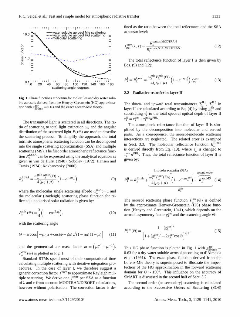
This HG phase function is plotted in Fig. 1 with gaer550 nm =

0.63 for a dry water soluble aerosol according to d’Almeidaet al. (1991). The exact phase function derived from theLorenz-Mie theory is superimposed to illustrate the imper-fection of the HG approximation in the forward scatteringdomain for Θ> 150◦. This influence on the accuracy ofSMART is discussed in the second half of Sect. 3.2.

The second order (or secondary) scattering is calculatedaccording to the Successive Orders of Scattering (SOS)method described by Hansen and Travis (1974):

Raer,MS(µ,µ0,φ−φ0) =τaerωaer

4π(16)

·2π∫0

1∫0

[1

µP aer

t (µ,µ′,φ−φ′)RSSA(µ′,µ0,φ′−φ0)

+1

µ0RSSA(µ,µ′,φ−φ′)P aer

t (µ′,µ0,φ′−φ0)

−e− τaer

µ0

µ0T SSA(µ,µ′,φ−φ′)P aer

r (µ′,µ0,φ′−φ0)

−e− τaer

µ

µP aer

r (µ,µ′,φ−φ′)T SSA(µ′,µ0,φ′−φ0)

]dµ′dφ′ .

Fig. 1. Phase functions at 550 nm for molecules and dry water solu-ble aerosols derived from the Henyey-Greenstein (HG) approxima-tion with gaer

550nm= 0.63 and the exact Lorenz-Mie theory.

The transmitted light is scattered in all directions. The ra-tio of scattering to total light extinctionωλ and the angulardistribution of the scattered lightPλ(2) are used to describethe scattering process. To simplify the approach, the totalintrinsic atmospheric scattering function can be decomposedinto the single scattering approximation (SSA) and multiplescattering (MS). The first order atmospheric reflectance func-tion R

I,SSAλ can be expressed using the analytical equation as

given in van de Hulst(1948); Sobolev(1972); Hansen andTravis(1974); Kokhanovsky(2006):

RI,SSAλ =

ωmlcλ P mlc

λ (2)

4(µ0+µ)

(1−e−mτ I

λ

), (9)

where the molecular single scattering albedoωmlcλ := 1 and

the molecular (Rayleigh) scattering phase function for re-flected, unpolarised solar radiation is given by:

P mlcλ (2) =

3

4

(1+cos22

), (10)

with the scattering angle

2 = arccos[−µ0µ+cos(φ−φ0)

√(1−µ0)(1−µ)

](11)

and the geometrical air mass factorm =

(µ−1

0 +µ−1).

P mlcλ (2) is plotted in Fig.1.Standard RTMs spend most of their computational time

calculating multiple scattering with iterative integration pro-cedures. In the case of layer I, we therefore suggest ageneric correction factorf corr to approximate Rayleigh mul-tiple scattering. We derive onef corr per SZA as a functionof λ andτ from accurate MODTRAN/DISORT calculations,however without polarisation. The correction factor is de-

fined as the ratio between the total reflectance and the SSAat sensor level:

f corrµ0

(λ,τ ) =R

sensor,MODTRANλ

Rsensor,SSA,MODTRANλ

. (12)

The total reflectance function of layer I is then given byEqs. (9) and (12):

RIλ = R

I,mlcλ =

ωmlcλ P mlc

λ (2)

4(µ0+µ)

(1−e−mτ I

λ

)f corr

µ0. (13)

2.2 Radiative transfer in layer II

The down- and upward total transmittancesTII ↓λ , T

II ↑λ in

layer II are calculated according to Eq. (4) by usinggaerλ and

substitutingτ Iλ to the total spectral optical depth of layer II

τ IIλ = τaer

λ +τmlcλ hPBL.

The atmospheric reflectance function of layer II is sim-plified by the decomposition into molecular and aerosolparts. As a consequence, the aerosol-molecule scatteringinteractions are neglected. The related error is examinedin Sect. 3.3. The molecular reflectance functionRII ,mlc

λ

is derived directly from Eq. (13), whereτ Iλ is changed to

τmlcλ hPBL. Thus, the total reflectance function of layer II is

given by:

RIIλ = R

II ,mlcλ +

first order scattering(SSA)︷︸︸︷ωaer

λ P aerλ (2r)

4(µ0+µ)

(1−e−mτaer

λ

)+

second order︷︸︸︷R

aer,MSλ︸︷︷︸

Raerλ

. (14)

The aerosol scattering phase functionP aerλ (2) is defined

by the approximate Henyey-Greenstein (HG) phase func-tion (Henyey and Greenstein, 1941), which depends on theaerosol asymmetry factorgaer

λ and the scattering angle2:

P aerλ (2) =

1−(gaer

λ

)2[1+

(gaer

λ

)2−2gaer

λ cos2]2/3

. (15)

This HG phase function is plotted in Fig.1 with gaer550nm=

0.63 for a dry water soluble aerosol according tod’Almeidaet al. (1991). The exact phase function derived from theLorenz-Mie theory is superimposed to illustrate the imper-fection of the HG approximation in the forward scatteringdomain for2 > 150◦. This influence on the accuracy ofSMART is discussed in the second half of Sect.3.2.

The second order (or secondary) scattering is calculatedaccording to the Successive Orders of Scattering (SOS)

www.atmos-meas-tech.net/3/1129/2010/ Atmos. Meas. Tech., 3, 1129–1141, 2010


method described byHansen and Travis(1974):

Raer,MS(µ,µ0,φ−φ0) =τaerωaer

4π(16)

·

2π∫0

1∫0

[1

µP aer

t

(µ,µ′,φ−φ′

)RSSA(µ′,µ0,φ

′−φ0

)+

1

µ0RSSA(µ,µ′,φ−φ′

)P aer

t

(µ′,µ0,φ

′−φ0

)−

e−

τaerµ0

µ0T SSA(µ,µ′,φ−φ′

)P aer

r

(µ′,µ0,φ

′−φ0

)−

e−

τaerµ

µP aer

r

(µ,µ′,φ−φ′

)T SSA(µ′,µ0,φ

′−φ0

)dµ′dφ′.

λ and other non-angular arguments are omitted for the sakeof readability. P aer

r andP aert denote the aerosol HG phase

function (Eq.15) using the scattering angle2r in case ofreflectance (Eq.11) and the scattering angle

2t = arccos[µ0µ+cos(φ−φ0)

√(1−µ0)(1−µ)

](17)

in case of transmittance. The single scattering transmit-tanceT SSA is given invan de Hulst(1948); Sobolev(1972);Hansen and Travis(1974); Kokhanovsky(2006):

T SSAλ =

ωaerλ P aer

λ (2t)

4(µ0−µ)

(e−

τaerλµ0 −e

−τaerλµ

). (18)

In case ofµ0=µ, we modify Eq. (18) to avoid indeterminacywith l’H opital’s (Bernoulli’s) rule:

T SSAλ =

ωaerλ P aer

λ (2t)

4µ2τaerλ e

(−

τaerλµ

). (19)

We use a numerical approximation to calculate the inte-grals of Eq. (16). This is by far the most computation-ally intensive step in SMART. Therefore, we currently ne-glect scattering orders higher than two. A third order termcould be added to Eq. (16) as given byHansen and Travis(1974). However, for our accuracy requirements and underfavourable remote sensing conditions, second order scatter-ing is sufficient. More details are given in the first half ofSect.3.2.

If fast computation is more important than accuracy,R

aer,MSλ can be substituted by·f corr

µ0

(λ,τaer

550nm

)in analogy to

Eq. (12). The expense is roughly 20% in decreased accuracy.

2.3 Radiative transfer at the surface

The modelling of optical processes at the surface can beelaborate due to adjacency and directional effects. Herewe assume the simple case with isotropically reflected lighton a homogeneous surface according to Lambert’s law(Angstrom, 1925; Chandrasekhar, 1960; Sobolev, 1972):

RSFCλ =

aλ

1−sλaλ

, (20)

where aλ is the surface albedo andsλ is the sphericalalbedo to account for multiple interaction between surfaceand atmosphere. We use the parameterization suggested byKokhanovsky et al.(2005) for sλ, where:

sλ = τ IIλ

(ae−

τ IIλα +be

−τ IIλβ +c

). (21)

The constantsa, α, b, β and c are parameterized accord-ing to Eq. (8). The corresponding expansion coefficients aregiven in Kokhanovsky et al.(2005). The resultingRSFC

λ isalso known as the hemispherical conical reflectance factor(HCRF) according toSchaepman-Strub et al.(2006).

2.4 At-sensor reflectance function

Finally, we put the above equations together along the opticalpath to resolve the reflectance functionRS

λ . Multiple retro-reflections between layers I and II are neglected. A sensor atTOA or within levels I or II is simulated as follows:

RS,TOAλ = RI

λ +TI↓λ

[RII

λ +RSFCλ T

II lλ

]T

I↑λ , (22)

RS,Iλ = RI

λshI+T

I↓λ

[RII

λ +RSFCλ T

II lλ

](1−shI

+shITI↑λ

), (23)

RS,IIλ = T

I↓λ

[RII

λ shII+T

II ↓λ RSFC

λ

(1−shII

+shIITII ↑λ

)]. (24)

whereTII lλ := T

II ↓λ T

II ↑λ ,

shI=

pPBL−pSensor

pPBL−pTOAand shII

=pSFC

−pSensor

pSFC−pPBL. (25)

These scaling factors are used to account for the relativeheight of the sensor within the corresponding layer.shI

ranges from 1 at TOA to 0 at the PBL, whileshII varies from1 at the PBL to 0 at the Earth’s surface (SFC).

3 Accuracy assessment

For typical airborne remote sensing conditions in the mid-latitudes we choose the representative uncertainty of imagingspectroscopy data of approximately 5% (Itten et al., 2008)as the accuracy requirement for SMART. Less typical con-ditions are analysed as well; in these cases we will acceptlarger errors. The definition of the conditions is given inTable1. The AOD range was chosen according to the find-ings ofRuckstuhl et al.(2008), the wavelength range selectedwith regard to the optimal sensor performance (Seidel et al.,2008), while also avoiding strong water vapour absorption.We assume a black surface at the sea level (aλ=0) to focus onthe atmospheric part of SMART. Furthermore, we solely usethe nadir viewing direction (µ=1), which is approximated bysmall field-of-view sensors (FOV<30◦).

This section evaluates if the prior accuracy require-ments can be met by SMART. We compare SMART with


F. C. Seidel et al.: Fast and simple model for atmospheric radiative transfer 1133

Table 1. Definition of the conditions and the related accuracy re-quirements for SMART. The limited conditions refer to typical air-borne remote sensing needs in the mid-latitudes, which SMARTwas developed for. The analysed conditions refer to the accuracyassessment.

remote sensing conditions limited analysed

τaer550nm 0–0.5 0–0.5

solar zenith angle, degrees 20–60 nadir–70viewing zenith angle nadir nadirwavelength, nm 500–700 400–800surface albedo 0 0accuracy requirement, % 5 15

an assumed virtual truth computed by the well knownRTM 6SV1.1. It accounts for polarisation and uses the SOSmethod as well as aerosol phase matrices based on Lorenz-Mie scattering theory (Vermote et al., 1997). It was validatedand found to be consistent to within 1% when compared toother RTMs byKotchenova et al.(2006). We use the de-fault accuracy mode of 6S with 48 Gaussian scattering anglesand 26 atmospheric layers. The use of more calculation an-gles and layers would be possible, but the accuracy increasewould be 0.4% at best (Kotchenova et al., 2006) and there-fore is negligible for our study. The two layers of SMARTwere chosen to interface at 2 km above the surface. The lowerlayer includes dry water soluble aerosols and molecules dis-tributed along the exponential vertical air pressure gradient.The corresponding aerosol optical parametersgaer

λ , ωaerλ and

αλ are taken fromd’Almeida et al.(1991) for SMART and6S. All results in this study are calculated with identical in-put parameters in SMART and in 6S, which are provided inTable2.

In the following, the accuracy of SMART is investigatedfor specific approximation uncertainties, as well as for theoverall accuracy. As an indicator of the accuracy, we calcu-late the relative difference or percent error of the reflectancefunction to the benchmark 6S:

δR ·100=RS

SMART−RS6S

RS6S

·100. (26)

3.1 Rayleigh scattering approximation and polarisation

The total Rayleigh scattering isRmlcλ = RmlcI

λ + RmlcIIλ as

given by Eqs. (13) and (14). The associated approxima-tions include the Rayleigh scattering phase function (Eq.10),the multiple scattering correction factor from MODTRAN(Eq.12) and the neglected polarisation due to the scalar equa-tions. The percent error is a distinct function of the wave-length and SZA, induced mainly by polarisation. Figure2ashows that it grows towards shorter wavelengths and larger


Table 2: Summary of the input parameters used in SMART and 6S for the accuracy assessment, with the aerosol and molecularoptical depth τaer

550 nm and τmlc550 nm, the solar and viewing zenith angle SZA and VZA, the aerosol asymmetry factor and single

scattering albedo gaer550 nm and ωaer

550 nm, the Angstrom parameter α550 nm, the surface albedo aλ, as well as the air pressure atthe surface and the planetary boundary layer pSFC and pPBL and the corresponding scaling factor hPBL.

parameter τaer550 nm τmlc

550nm SZA VZA gaer550 nm ωaer

550 nm α550 nm aλ pSFC pPBL hPBL

value 0–0.5 0.097 nadir–70◦ nadir 0.638 0.963 1.23 0 1013 mb 800 mb 0.211

the nadir viewing direction (µ=1), which is approximated bysmall field-of-view sensors (FOV<30◦).

This section evaluates if the prior accuracy require-ments can be met by SMART. We compare SMART withan assumed virtual truth computed by the well knownRTM 6SV1.1. It accounts for polarisation and uses the SOSmethod as well as aerosol phase matrices based on Lorenz-Mie scattering theory (Vermote et al., 1997). It was validatedand found to be consistent to within 1% when compared toother RTMs by Kotchenova et al. (2006). We use the de-fault accuracy mode of 6S with 48 Gaussian scattering anglesand 26 atmospheric layers. The use of more calculation an-gles and layers would be possible, but the accuracy increasewould be 0.4% at best (Kotchenova et al., 2006) and there-fore is negligible for our study. The two layers of SMARTwere chosen to interface at 2 km above the surface. The lowerlayer includes dry water soluble aerosols and molecules dis-tributed along the exponential vertical air pressure gradient.The corresponding aerosol optical parameters gaer

λ , ωaerλ and

αλ are taken from d’Almeida et al. (1991) for SMART and6S. All results in this study are calculated with identical in-put parameters in SMART and in 6S, which are provided inTable 2.

In the following, the accuracy of SMART is investigatedfor specific approximation uncertainties, as well as for theoverall accuracy. As an indicator of the accuracy, we calcu-late the relative difference or percent error of the reflectancefunction to the benchmark 6S:

δR ·100 =RS

SMART−RS6S

RS6S

·100. (26)

3.1 Rayleigh scattering approximation and polarisation

The total Rayleigh scattering is Rmlcλ =RmlcI

λ +RmlcIIλ as

given by Eqs. (13) and (14). The associated approxima-tions include the Rayleigh scattering phase function (Eq. 10),the multiple scattering correction factor from MODTRAN(Eq. 12) and the neglected polarisation due to the scalar equa-tions. The percent error is a distinct function of the wave-length and SZA, induced mainly by polarisation. Figure 2ashows that it grows towards shorter wavelengths and largerSZA. It is known that the scalar approximation can introduce

rela

tive

err

or,

%

10

5

0

−5

−10

wavelength, nm800750700650600550500450400

SZA=60SZA=45SZA=30SZA=15

(a) δRmlcλ (λ) ·100

rela

tive

err

or,

%

10

5

0

−5

−10

solar zenith angle, degrees706050403020100

AOD=0.0

(b) δRmlc550 nm(SZA) ·100 at λ=550 nm

Fig. 2: Percent error due to Rayleigh scattering and polarisa-tion with respect to wavelength and solar zenith angle (SZA)at top-of-atmosphere.

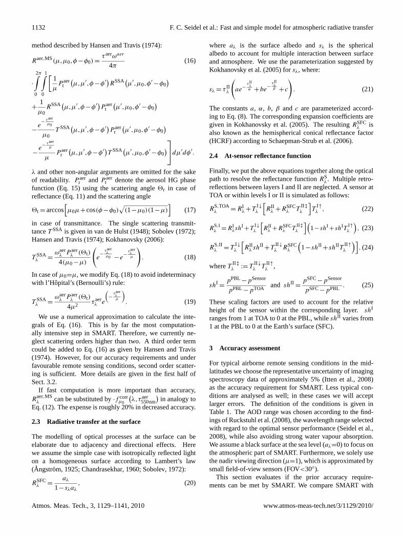
uncertainties of up to 10% in the blue spectral region (vande Hulst, 1980; Mishchenko et al., 1994). The SZA depen-dency of this uncertainty is shown in Fig. 2b. At 550 nm,the Rayleigh scattering uncertainty in the typical SZA rangefrom 20–50◦ is below 3%.

Fig. 2. Percent error due to Rayleigh scattering and polarisationwith respect to wavelength and solar zenith angle (SZA) at top-of-atmosphere.

SZA. It is known that the scalar approximation can introduceuncertainties of up to 10% in the blue spectral region (vande Hulst, 1980; Mishchenko et al., 1994). The SZA depen-dency of this uncertainty is shown in Fig.2b. At 550 nm,the Rayleigh scattering uncertainty in the typical SZA rangefrom 20–50◦ is below 3%.

3.2 Aerosol scattering approximation

The main approximations for the aerosol scattering arethe double scattering (Eq.16) and the HG phase function(Eq. 15). Initially, we use the exactly same phase functionas in 6S in order to study the error induced only by the ne-glected higher orders of scattering. This phase function fordry water soluble aerosols was derived from the Lorenz-Miescattering theory. Subsequently, we compare the combined



Table 2. Summary of the input parameters used in SMART and 6S for the accuracy assessment, with the aerosol and molecular optical depthτaer550nmandτmlc

550nm, the solar and viewing zenith angle SZA and VZA, the aerosol asymmetry factor and single scattering albedogaer550nm

andωaer550nm, theAngstrom parameterα550nm, the surface albedoaλ, as well as the air pressure at the surface and the planetary boundary

layerpSFCandpPBL and the corresponding scaling factorhPBL.

parameter τaer550nm τmlc

550nm SZA VZA gaer550nm ωaer

550nm α550nm aλ pSFC pPBL hPBL

value 0–0.5 0.097 nadir–70◦ nadir 0.638 0.963 1.23 0 1013 mb 800 mb 0.211

effect of the double scattering and the HG phase function ap-proximation with 6S.

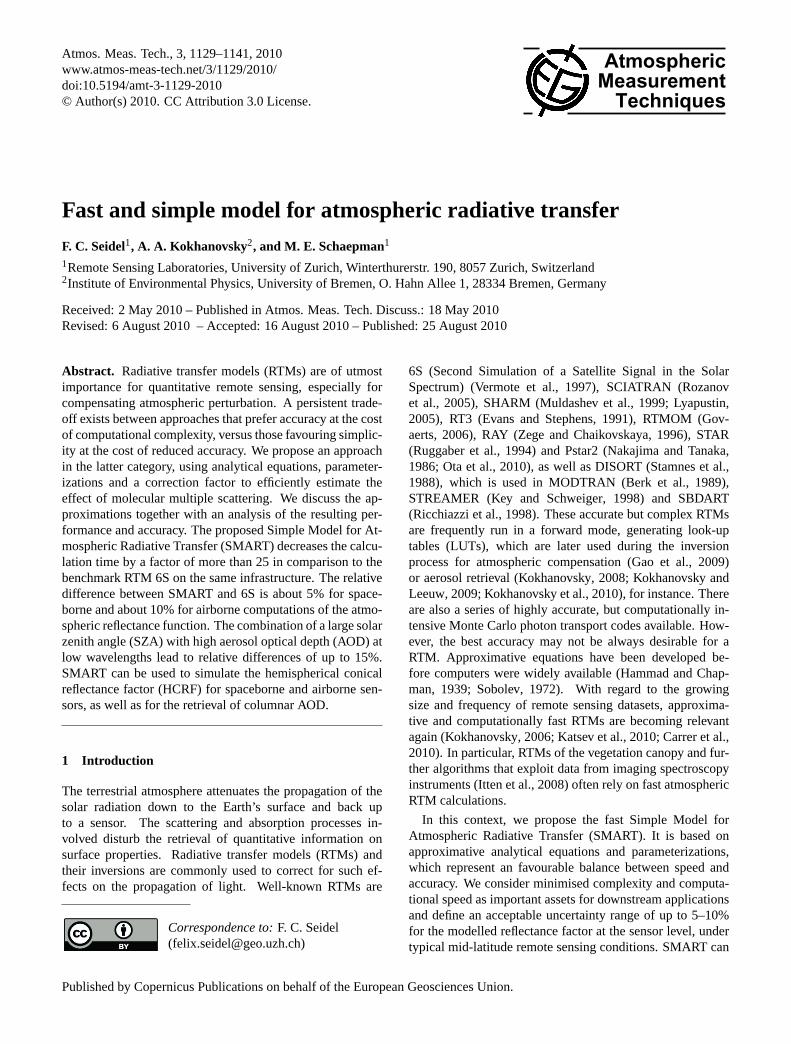
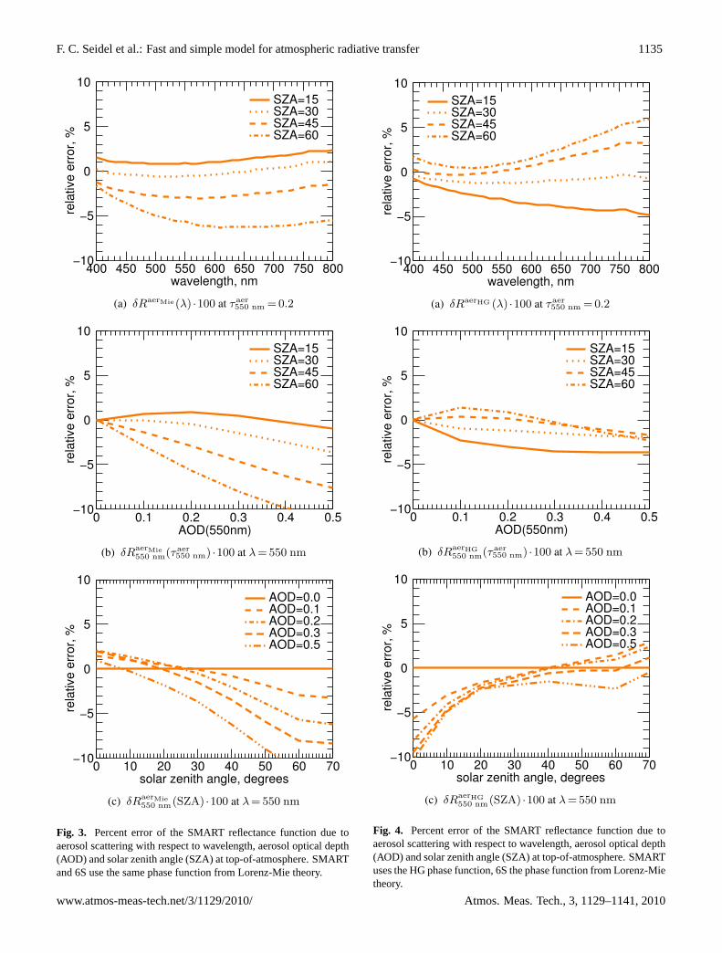
The percent error introduced by the double scattering ap-proximation is plotted in Fig.3. It is almost constant over thespectra due to the higher reflectance at shorter wavelengths(see Fig.3a). It is obvious that the reflectance functionRS

λ isincreasingly underestimated by SMART for larger AOD dueto the neglected third and higher orders of aerosol scattering(see Fig.3b). Figure3c shows that larger SZA leads to anunderestimation of the atmospheric reflectance for the samereason.

In order to study the accuracy of the total aerosol scatter-ing Raer

λ as part of Eq. (14), we include the approximativeHG phase function in SMART. 6S still uses the same Miephase function as before. The input parameter for the HGphase functiongaer

λ corresponds to the same dry water sol-uble aerosol, which is used in 6S. The exact Mie and theapproximative HG phase function are shown in Fig.1 for thesame aerosol. The latter provides a reasonable approxima-tion for scattering angles around 130◦, which corresponds toa 50◦ SZA for nadir observations. The resulting combinationof the aerosol double scattering error with the HG approxi-mation error is examined in Fig.4. It suggests that the useof the HG approximation does not introduce large percent er-rors within the range of typical SZA, as defined in Table1.Given a range of 20–45◦ SZA, SMART is quite accurate atall investigated wavelengths and AOD values.

By comparing Figs.3a with4a and Figs.3b with 4b, it canbe seen that the HG approximation reverses some of the er-rors due to the aerosol double scattering approximation. TheHG phase function for dry water soluble aerosols tends tooverestimate of the aerosol scattering, which finally leads toa less distinct underestimation due to the neglected third andhigher orders of aerosol scattering.

3.3 Coupling of Rayleigh and aerosol scattering

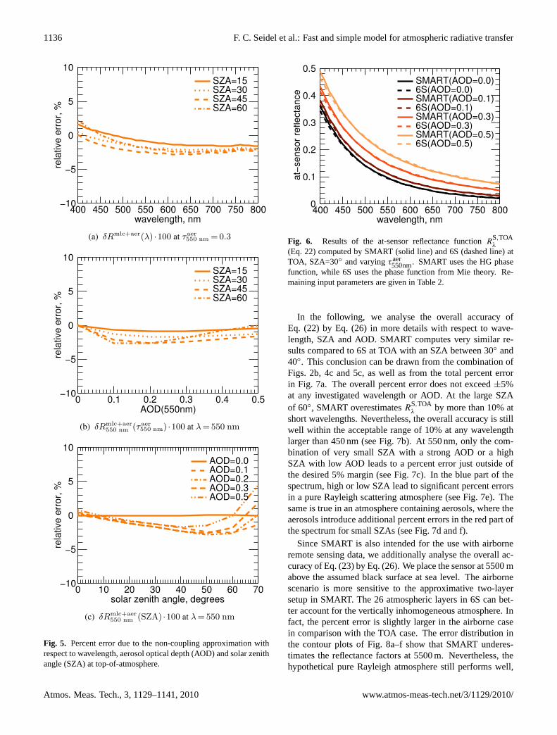
The current version of SMART does not yet account for thescattering interaction between molecules and aerosols. Weanalyse this effect by comparing 6S computations with thecoupling switched on and off. The relative error related tothis specific approximation is shown in Fig.5. It remainswithin about 3%, reaching a maximum at large SZA (seeFig. 5c) and short wavelengths (see Fig.5a). With errors

of less than 2%, small SZAs are almost not influenced by thecoupling and there is no distinct dependency on AOD notice-able (see Fig.5b).

3.4 Overall accuracy

Previous Sects.3.1–3.3 demonstrated that the approxima-tions in SMART are adequate. Most of them are within thedesired accuracy range of±5% for the limited remote sens-ing conditions as defined in Table1. Errors of up to±15%are found for large SZA, however, they are mainly related toSMART’s simple two-layer atmospheric structure.

In the following, we examine the overall accuracy ofSMART by comparing it according to Eq. (26) with inde-pendent computations of 6S. The computations of SMARTare performed by Eq. (22) for a TOA sensor altitude at 80 kmand by Eq. (23) for an airborne sensor altitude at 5500 m a.s.l.The percent error due to the excluded coupling betweenmolecules and aerosols is inherent in the results of this sub-section.

Figure6 shows the result of two independent calculationsusing SMART (solid line) and 6S (dashed line) with respectto λ andτaer

550nm. The qualitative agreement between the twomodels is evident. A quantitative perspective by statisticalmeans of the overall accuracy is provided in Table3, where

R2= 1−

∑(RS

SMART−RS6S

)2∑(

RS6S− RS

6S

)2, (27)

is the squared correlation coefficient between the twomodels,

RMSE=

√1

N

∑(RS

SMART−RS6S

)2, (28)

is the root mean square error and

NRMSE=RMSE·100

max(RS

SMART

)−min

(RS

SMART

) , (29)

is the normalised RMSE. The statistics are derived from allcombinations of input parameters defined in Tables1 and2within the limited conditions. The resulting correlation be-tween SMART and 6S is almost perfect. The RMSE is ap-proximately 0.16 reflectance values and the NRMSE is be-tween 1.8% and 3.5%. The differences are smaller at TOA incomparison to those at 5500 m.


F. C. Seidel et al.: Fast and simple model for atmospheric radiative transfer 11356 F. C. Seidel et al.: Fast and simple model for atmospheric radiative transfer

3.2 Aerosol scattering approximation

The main approximations for the aerosol scattering arethe double scattering (Eq. 16) and the HG phase function(Eq. 15). Initially, we use the exactly same phase functionas in 6S in order to study the error induced only by the ne-glected higher orders of scattering. This phase function fordry water soluble aerosols was derived from the Lorenz-Miescattering theory. Subsequently, we compare the combinedeffect of the double scattering and the HG phase function ap-proximation with 6S.

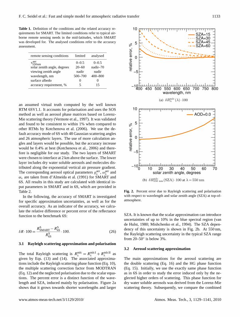
The percent error introduced by the double scattering ap-proximation is plotted in Fig. 3. It is almost constant over thespectra due to the higher reflectance at shorter wavelengths(see Fig. 3a). It is obvious that the reflectance function RS

λ isincreasingly underestimated by SMART for larger AOD dueto the neglected third and higher orders of aerosol scattering(see Fig. 3b). Figure 3c shows that larger SZA leads to anunderestimation of the atmospheric reflectance for the samereason.

In order to study the accuracy of the total aerosol scatter-ing Raer

λ as part of Eq. (14), we include the approximativeHG phase function in SMART. 6S still uses the same Miephase function as before. The input parameter for the HGphase function gaer

λ corresponds to the same dry water sol-uble aerosol, which is used in 6S. The exact Mie and theapproximative HG phase function are shown in Fig. 1 for thesame aerosol. The latter provides a reasonable approxima-tion for scattering angles around 130◦, which corresponds toa 50◦ SZA for nadir observations. The resulting combinationof the aerosol double scattering error with the HG approxi-mation error is examined in Fig. 4. It suggests that the useof the HG approximation does not introduce large percent er-rors within the range of typical SZA, as defined in Table 1.Given a range of 20–45◦ SZA, SMART is quite accurate atall investigated wavelengths and AOD values.

By comparing Fig. 3a with 4a and Fig. 3b with 4b, it canbe seen that the HG approximation reverses some of the er-rors due to the aerosol double scattering approximation. TheHG phase function for dry water soluble aerosols tends tooverestimate of the aerosol scattering, which finally leads toa less distinct underestimation due to the neglected third andhigher orders of aerosol scattering.

3.3 Coupling of Rayleigh and aerosol scattering

The current version of SMART does not yet account for thescattering interaction between molecules and aerosols. Weanalyse this effect by comparing 6S computations with thecoupling switched on and off. The relative error related tothis specific approximation is shown in Fig. 5. It remainswithin about 3%, reaching a maximum at large SZA (seeFig. 5c) and short wavelengths (see Fig. 5a). With errorsof less than 2%, small SZAs are almost not influenced by the

rela

tive e

rror,

%10

5

0

−5

−10

wavelength, nm800750700650600550500450400


(a) δRaerMie(λ) ·100 at τaer550 nm =0.2

rela

tive e

rror,

%

10

5

0

−5

−10

AOD(550nm)0.50.40.30.20.10


(b) δRaerMie550 nm(τaer

550 nm) ·100 at λ= 550 nm

rela

tive e

rror,

%

10

5

0

−5

−10


AOD=0.5AOD=0.3AOD=0.2AOD=0.1AOD=0.0

(c) δRaerMie550 nm(SZA) ·100 at λ=550 nm

Fig. 3: Percent error of the SMART reflectance function dueto aerosol scattering with respect to wavelength, aerosol op-tical depth (AOD) and solar zenith angle (SZA) at top-of-atmosphere. SMART and 6S use the same phase functionfrom Lorenz-Mie theory.

Fig. 3. Percent error of the SMART reflectance function due toaerosol scattering with respect to wavelength, aerosol optical depth(AOD) and solar zenith angle (SZA) at top-of-atmosphere. SMARTand 6S use the same phase function from Lorenz-Mie theory.


rela

tive

err

or,

%

10

5

0

−5

−10

wavelength, nm800750700650600550500450400


(a) δRaerHG (λ) ·100 at τaer550 nm =0.2

rela

tive

err

or,

%

10

5

0

−5

−10

AOD(550nm)0.50.40.30.20.10


(b) δRaerHG550 nm(τaer

550 nm) ·100 at λ=550 nm

rela

tive

err

or,

%

10

5

0

−5

−10



(c) δRaerHG550 nm(SZA) ·100 at λ=550 nm

Fig. 4: Percent error of the SMART reflectance function dueto aerosol scattering with respect to wavelength, aerosol op-tical depth (AOD) and solar zenith angle (SZA) at top-of-atmosphere. SMART uses the HG phase function, 6S thephase function from Lorenz-Mie theory.

rela

tive

err

or,

%

10

5

0

−5

−10

wavelength, nm800750700650600550500450400


(a) δRmlc+aer(λ) ·100 at τaer550 nm =0.3

rela

tive

err

or,

%

10

5

0

−5

−10

AOD(550nm)0.50.40.30.20.10


(b) δRmlc+aer550 nm (τaer

550 nm) ·100 at λ= 550 nm

rela

tive

err

or,

%

10

5

0

−5

−10



(c) δRmlc+aer550 nm (SZA) ·100 at λ=550 nm

Fig. 5: . Percent error due to the non-coupling approximationwith respect to wavelength, aerosol optical depth (AOD) andsolar zenith angle (SZA) at top-of-atmosphere.

Fig. 4. Percent error of the SMART reflectance function due toaerosol scattering with respect to wavelength, aerosol optical depth(AOD) and solar zenith angle (SZA) at top-of-atmosphere. SMARTuses the HG phase function, 6S the phase function from Lorenz-Mietheory.


1136 F. C. Seidel et al.: Fast and simple model for atmospheric radiative transferF. C. Seidel et al.: Fast and simple model for atmospheric radiative transfer 7

rela

tive e

rror,

%

10

5

0

−5

−10

wavelength, nm800750700650600550500450400


(a) δRaerHG (λ) ·100 at τaer550 nm =0.2

rela

tive e

rror,

%

10

5

0

−5

−10

AOD(550nm)0.50.40.30.20.10


(b) δRaerHG550 nm(τaer

550 nm) ·100 at λ=550 nm

rela

tive e

rror,

%

10

5

0

−5

−10



(c) δRaerHG550 nm(SZA) ·100 at λ=550 nm

Fig. 4: Percent error of the SMART reflectance function dueto aerosol scattering with respect to wavelength, aerosol op-tical depth (AOD) and solar zenith angle (SZA) at top-of-atmosphere. SMART uses the HG phase function, 6S thephase function from Lorenz-Mie theory.

rela

tive e

rror,

%10

5

0

−5

−10

wavelength, nm800750700650600550500450400


(a) δRmlc+aer(λ) ·100 at τaer550 nm = 0.3

rela

tive e

rror,

%

10

5

0

−5

−10

AOD(550nm)0.50.40.30.20.10


(b) δRmlc+aer550 nm (τaer

550 nm) ·100 at λ=550 nm

rela

tive e

rror,

%

10

5

0

−5

−10



(c) δRmlc+aer550 nm (SZA) ·100 at λ= 550 nm

Fig. 5: . Percent error due to the non-coupling approximationwith respect to wavelength, aerosol optical depth (AOD) andsolar zenith angle (SZA) at top-of-atmosphere.

Fig. 5. Percent error due to the non-coupling approximation withrespect to wavelength, aerosol optical depth (AOD) and solar zenithangle (SZA) at top-of-atmosphere.


coupling and there is no distinct dependency on AOD notice-able (see Fig. 5b).

3.4 Overall accuracy

Previous Sects. 3.1–3.3 demonstrated that the approxima-tions in SMART are adequate. Most of them are within thedesired accuracy range of ±5% for the limited remote sens-ing conditions as defined in Table 1. Errors of up to ±15%are found for large SZA, however, they are mainly related toSMART’s simple two-layer atmospheric structure.

In the following, we examine the overall accuracy ofSMART by comparing it according to Eq. (26) with inde-pendent computations of 6S. The computations of SMARTare performed by Eq. (22) for a TOA sensor altitude at 80 kmand by Eq. (23) for an airborne sensor altitude at 5500 m a.s.l.The percent error due to the excluded coupling betweenmolecules and aerosols is inherent in the results of this sub-section.

Figure 6 shows the result of two independent calculationsusing SMART (solid line) and 6S (dashed line) with respectto λ and τaer

550 nm. The qualitative agreement between the twomodels is evident. A quantitative perspective by statisticalmeans of the overall accuracy is provided in Table 3, where

R2 = 1−∑(

RSSMART−RS

6S

)2∑(RS

6S−RS6S

)2 , (27)

is the squared correlation coefficient between the two mod-els,

RMSE =

√1

N

∑(RS

SMART−RS6S

)2, (28)

is the root mean square error and

NRMSE =RMSE ·100

max(RS

SMART

)−min

(RS

SMART

) , (29)

is the normalised RMSE. The statistics are derived from allcombinations of input parameters defined in Tables 1 and 2within the limited conditions. The resulting correlation be-tween SMART and 6S is almost perfect. The RMSE is ap-proximately 0.16 reflectance values and the NRMSE is be-tween 1.8% and 3.5%. The differences are smaller at TOA incomparison to those at 5500 m.

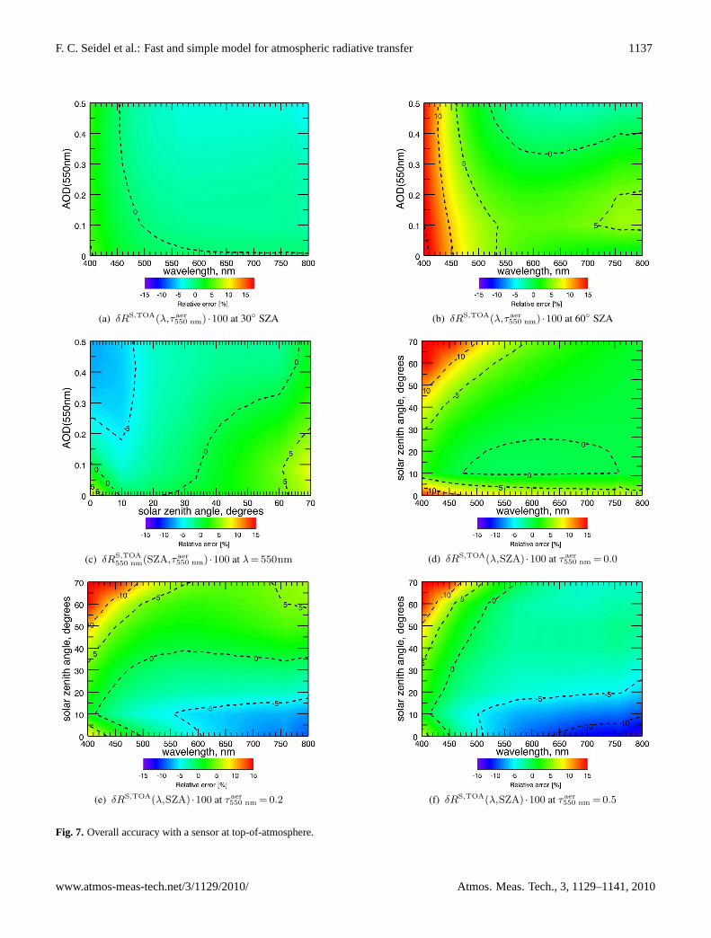
In the following, we analyse the overall accuracy ofEq. (22) by Eq. (26) in more details with respect to wave-length, SZA and AOD. SMART computes very similar re-sults compared to 6S at TOA with an SZA between 30◦ and40◦. This conclusion can be drawn from the combination ofFigs. 2b, 4c and 5c, as well as from the total percent errorin Fig. 7a. The overall percent error does not exceed ±5%at any investigated wavelength or AOD. At the large SZAof 60◦, SMART overestimates RS,TOA

λ by more than 10%at short wavelengths. Nevertheless, the overall accuracy is

Table 3: Quantitative comparison between SMART and 6Sby statistical means for the limited conditions as defined inTable 1. SMART uses the HG phase function; 6S usedthe phase function from Mie calculations. R2 denotes thesquared correlation coefficient, RMSE the root mean squareerror and NRMSE the normalised RMSE.

sensor altitude R2 RMSE NRMSE

TOA 0.998 0.157 1.77%

5500 m 0.998 0.167 3.52%

at−

sensor

reflecta

nce

0.5

0.4

0.3

0.2

0.1

0

wavelength, nm800750700650600550500450400

6S(AOD=0.5)SMART(AOD=0.5)6S(AOD=0.3)SMART(AOD=0.3)6S(AOD=0.1)SMART(AOD=0.1)6S(AOD=0.0)SMART(AOD=0.0)

Fig. 6: Results of the at-sensor reflectance function RS,TOAλ

(Eq. 22) computed by SMART (solid line) and 6S (dashedline) at TOA, SZA=30◦ and varying τaer

550 nm. SMART usesthe HG phase function, while 6S uses the phase functionfrom Mie theory. Remaining input parameters are given inTable 2.

still well within the acceptable range of 10% at any wave-length larger than 450 nm (see Fig. 7b). At 550 nm, only thecombination of very small SZA with a strong AOD or a highSZA with low AOD leads to a percent error just outside ofthe desired 5% margin (see Fig. 7c). In the blue part of thespectrum, high or low SZA lead to significant percent errorsin a pure Rayleigh scattering atmosphere (see Fig. 7e). Thesame is true in an atmosphere containing aerosols, where theaerosols introduce additional percent errors in the red part ofthe spectrum for small SZAs (see Figs. 7d and 7f).

Since SMART is also intended for the use with airborneremote sensing data, we additionally analyse the overall ac-curacy of Eq. (23) by Eq. (26). We place the sensor at 5500 mabove the assumed black surface at sea level. The airbornescenario is more sensitive to the approximative two-layersetup in SMART. The 26 atmospheric layers in 6S can bet-ter account for the vertically inhomogeneous atmosphere. In

Fig. 6. Results of the at-sensor reflectance functionRS,TOAλ

(Eq. 22) computed by SMART (solid line) and 6S (dashed line) atTOA, SZA=30◦ and varyingτaer

550nm. SMART uses the HG phasefunction, while 6S uses the phase function from Mie theory. Re-maining input parameters are given in Table 2.

In the following, we analyse the overall accuracy ofEq. (22) by Eq. (26) in more details with respect to wave-length, SZA and AOD. SMART computes very similar re-sults compared to 6S at TOA with an SZA between 30◦ and40◦. This conclusion can be drawn from the combination ofFigs. 2b, 4c and5c, as well as from the total percent errorin Fig. 7a. The overall percent error does not exceed±5%at any investigated wavelength or AOD. At the large SZAof 60◦, SMART overestimatesRS,TOA

λ by more than 10% atshort wavelengths. Nevertheless, the overall accuracy is stillwell within the acceptable range of 10% at any wavelengthlarger than 450 nm (see Fig.7b). At 550 nm, only the com-bination of very small SZA with a strong AOD or a highSZA with low AOD leads to a percent error just outside ofthe desired 5% margin (see Fig.7c). In the blue part of thespectrum, high or low SZA lead to significant percent errorsin a pure Rayleigh scattering atmosphere (see Fig.7e). Thesame is true in an atmosphere containing aerosols, where theaerosols introduce additional percent errors in the red part ofthe spectrum for small SZAs (see Fig.7d and f).

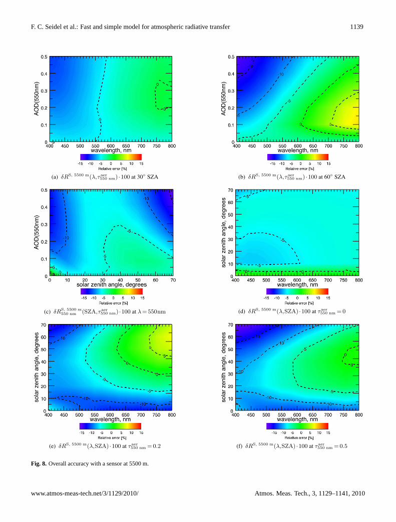
Since SMART is also intended for the use with airborneremote sensing data, we additionally analyse the overall ac-curacy of Eq. (23) by Eq. (26). We place the sensor at 5500 mabove the assumed black surface at sea level. The airbornescenario is more sensitive to the approximative two-layersetup in SMART. The 26 atmospheric layers in 6S can bet-ter account for the vertically inhomogeneous atmosphere. Infact, the percent error is slightly larger in the airborne casein comparison with the TOA case. The error distribution inthe contour plots of Fig.8a–f show that SMART underes-timates the reflectance factors at 5500 m. Nevertheless, thehypothetical pure Rayleigh atmosphere still performs well,




(a) δRS,TOA(λ,τaer550 nm) ·100 at 30◦ SZA (b) δRS,TOA(λ,τaer

550 nm) ·100 at 60◦ SZA

(c) δRS,TOA550 nm(SZA,τaer

550 nm) ·100 at λ=550nm (d) δRS,TOA(λ,SZA) ·100 at τaer550 nm = 0.0

(e) δRS,TOA(λ,SZA) ·100 at τaer550 nm =0.2 (f) δRS,TOA(λ,SZA) ·100 at τaer

550 nm =0.5

Fig. 7: Overall accuracy with a sensor at top-of-atmosphere.Fig. 7. Overall accuracy with a sensor at top-of-atmosphere.



Table 3. Quantitative comparison between SMART and 6S bystatistical means for the limited conditions as defined in Table1.SMART uses the HG phase function; 6S used the phase functionfrom Mie calculations.R2 denotes the squared correlation coef-ficient, RMSE the root mean square error and NRMSE the nor-malised RMSE.

sensor altitude R2 RMSE NRMSE

TOA 0.998 0.157 1.77%

5500 m 0.998 0.167 3.52%

with a maximum percent error of 6% (see Fig.8a, b and c).The aerosols worsen the underestimation in the lower half ofthe visible spectrum, especially at very small and very largeSZAs. At 550 nm and a 30◦ SZA, the percent error is 6%or less for an AOD up to 0.5. With the same constellationbut an extreme SZA, the percent errors reach about 10% (seeFig. 8c, e and f). The largest offset between SMART and 6Sis found at 60◦ SZA, 400 nm and an AOD of 0.5 with 18%relative difference. However, it should be noted that absolutedifferenceRS

SMART −RS6S is in fact smaller in the airborne

case compared to the TOA case (not shown). Nonetheless,the relative error given by Eq. (26) is larger due to the smallerRS

6S in the denominator.

4 Performance assessment

SMART is designed to optimally balance the opposing needsfor accuracy and computational speed; the speed decreaseswith increasing model complexity and accuracy. We use the6S vector version 1.1 (Vermote et al., 1997) as a benchmarkRTM (same as in Sect.3) to assesses the performance ofSMART. 6S is compiled with GNU Fortran and SMART isimplemented in IDL. Both run on the same CPU infrastruc-ture.

SMART needs only approximately 0.05 s for the calcu-lation of one reflectance factor value. The more com-plex 6S needs about 1.4 s under identical conditions. Con-sequently, SMART computes more than 25 times faster. IfR

aer,MSλ (Eq. 16) is substituted by a simple correction factor

f corrµ0

(λ,τ ) for aerosol multiple scattering (similar to Eq.12),SMART runs 220 times faster than by numerically solvingEq. (16) in the presented configuration.

5 Summary and conclusions

We introduced SMART, as well as its approximative radia-tive transfer equations and parameterizations. Results ofthe atmospheric at-sensor reflectance function computed bySMART were compared with benchmark results from 6S for

accuracy and performance. The overall percent error was ex-amined and discussed, as were the individual errors resultingfrom Rayleigh scattering, aerosol scattering and molecule-aerosol interactions. The aerosol scattering was comparedto 6S with and without the effect of the HG phase functionapproximation.

We found that SMART fulfils its design principle: it is fastand simple, yet accurate enough for a range of applications.One example may include the assessment of atmospheric ef-fects when inspecting the quality of airborne or spacebornedata against ground truth measurements in near-real-time.The generation of atmospheric input parameters for vegeta-tion canopy RTM inversion schemes, could be another appli-cation. SMART computes more than 20 reflectance resultsper second on a current customary desktop computer. Thisis more than 25 times faster than the benchmark RTM. Theoverall percent error under typical mid-latitude remote sens-ing conditions was found to be about 5% for the spaceborneand 5% to 10% for the airborne case. Large AOD or SZAvalues lead to larger percent errors of up to 15%. In gen-eral, the included approximations are sensitive to the strongscattering in the blue spectral region, which leads to largerpercent errors. Together with the effect of polarisation, thetotal percent error of SMART exceeds the desired accuracygoal of 5% only in the blue region. It is therefore suggestedthat SMART be used preferably in the spectral range betweenroughly 500 nm and 680 nm, avoiding the blue and strong ab-sorption bands. However, the neglected ozone absorption inthis spectral interval leads to a small overestimation of upto 0.007 reflectance units at large SZA and 600 nm. It is alsorecommended to use SMART for computations with a sensorabove the PBL to avoid uncertainties in the vertical distribu-tion of the aerosols.

SMART can be improved by implementing other phasefunctions instead of the HG approximation, including thosederived from Lorenz-Mie theory, geometrical optics (ray-tracing), and T-matrix approaches (Liou and Hansen, 1971;Mishchenko et al., 2002). Further refinements may includethe coupling between molecules and aerosols, as well asthe implementation of freely mixable aerosol componentsand hygroscopic growth (Hess et al., 1998). To accountfor polarisation, the scalar equations can be extended to thevector notation. Furthermore, a similar approach as usedfor the Rayleigh multiple scattering in this study (Eq.12)may perhaps be used to perform a rough polarisation cor-rection. Other issues for further developments may includeadditional atmospheric layers, gaseous absorption (foremostozone), adjacency effects and the treatment of a directional,non-Lambertian surface.

A recent inter-comparison study for classic RTMs such as6S, RT3, MODTRAN and SHARM, found discrepancies ofδR≤5% at TOA (Kotchenova et al., 2008). Even larger errorswere found when polarisation was neglected or the HG phasefunction was used. SMART does not yet account for polari-sation and uses the HG approximation by default, however




(a) δRS, 5500 m(λ,τaer550 nm) ·100 at 30◦ SZA (b) δRS, 5500 m(λ,τaer

550 nm) ·100 at 60◦ SZA

(c) δRS, 5500 m550 nm (SZA,τaer

550 nm) ·100 at λ=550nm (d) δRS, 5500 m(λ,SZA) ·100 at τaer550 nm =0

(e) δRS, 5500 m(λ,SZA) ·100 at τaer550 nm =0.2 (f) δRS, 5500 m(λ,SZA) ·100 at τaer

550 nm =0.5

Fig. 8: Overall accuracy with a sensor at 5500 m.Fig. 8. Overall accuracy with a sensor at 5500 m.



with the option to include pre-calculated Mie phase func-tions. Therefore, the overall accuracy achieved by SMARTunder given conditions can be regarded as satisfactory, espe-cially when a computationally fast RTM is required.

Acknowledgements.The work of A. A. Kokhanovsky was per-formed in the framework of DFG Project Terra. Suggestions fromD. Schlaepfer and A. Schubert were very much appreciated. Wethank three anonymous referees for their valuable comments on theAMTD version of this publication.

Edited by: M. Wendisch

References

Angstrom, A.: The albedo of various surfaces of ground, Ge-ogr. Ann., 7, 323–342, available at:http://www.jstor.org/stable/519495, last access: 1 May 2010, 1925.

Angstrom, A.: On the atmospheric transmission of sun radiationand on dust in the air, Geogr. Ann., 11, 156–166, availableat: http://www.jstor.org/stable/519399, last access: 1 May 2010,1929.

Berk, A., Bernstein, L., and Robertson, D.: MODTRAN: a mod-erate resolution model for LOWTRAN7, Tech. Rep. GL-TR-89-0122, Air Force Geophysics Lab, Hanscom AFB, Massachusetts,USA, 1989.

Bodhaine, B. A., Wood, N. B., Dutton, E. G., and Slusser,J. R.: On Rayleigh optical depth calculations, J. At-mos. Ocean. Tech., 16, 1854–1861, doi:10.1175/1520-0426(1999)016<1854:ORODC>2.0.CO;2, 1999.

Carrer, D., Roujean, J.-L., Hautecoeur, O., and Elias, T.:Daily estimates of aerosol optical thickness over land sur-face based on a directional and temporal analysis of SEVIRIMSG visible observations, J. Geophys. Res., 115, D10208,doi:10.1029/2009JD012272, 2010.

Chandrasekhar, S.: Radiative Transfer, Dover, New York, USA,1960.

d’Almeida, G., Koepke, P., and Shettle, E.: Atmospheric aerosols:global climatology and radiative characteristics, Deepak, Hamp-ton, Virginia, USA, 1991.

Evans, K. F. and Stephens, G. L.: A new polarized atmosphericradiative transfer model, J. Quant. Spectrosc. Ra., 46, 413–423,doi:10.1016/0022-4073(91)90043-P, 1991.

Gao, B.-C., Montes, M. J., Davis, C. O., and Goetz, A. F. H.: Atmo-spheric correction algorithms for hyperspectral remote sensingdata of land and ocean, Remote Sens. Environ., 113, S17–S24,doi:10.1016/j.rse.2007.12.015, 2009.

Govaerts, Y.: RTMOM V0B.10 Evaluation report, reportEUM/MET/DOC/06/0502, EUMETSAT, 2006.

Hammad, A. and Chapman, S.: VII. The primary and sec-ondary scattering of sunlight in a plane-stratified atmosphereof uniform composition, Philos. Mag., 28, 99–110, availableat: http://articles.adsabs.harvard.edu//full/1948ApJ...108..338H/0000338.000.html, last access: 1 May 2010, 1939.

Hansen, J. E. and Travis, L. D.: Light scattering inplanetary atmospheres, Space Sci. Rev., 16, 527–610,doi:10.1007/BF00168069, 1974.

Henyey, L. and Greenstein, J.: Diffuse radiation in the galaxy, As-trophys. J., 93, 70–83, available at:http://articles.adsabs.harvard.edu/full/1940AnAp....3..117H, last access: 1 May 2010, 1941.

Hess, M., Koepke, P., and Schult, I.: Optical properties of aerosolsand clouds: the software package OPAC, B. Am. Meteorol. Soc.,79, 831–844, 1998.

Itten, K. I., Dell’Endice, F., Hueni, A., Kneubuhler, M., Schlapfer,D., Odermatt, D., Seidel, F., Huber, S., Schopfer, J., Kellen-berger, T., Buhler, Y., D’Odorico, P., Nieke, J., Alberti, E., andMeuleman, K.: APEX – the hyperspectral ESA airborne prismexperiment, Sensors, 8, 6235–6259, doi:10.3390/s8106235,available at: http://www.mdpi.com/1424-8220/8/10/6235, lastaccess: 1 May 2010, 2008.

Katsev, I. L., Prikhach, A. S., Zege, E. P., Grudo, J. O., andKokhanovsky, A. A.: Speeding up the AOT retrieval procedureusing RTT analytical solutions: FAR code, Atmos. Meas. Tech.Discuss., 3, 1645–1705, doi:10.5194/amtd-3-1645-2010, 2010.

Key, J. and Schweiger, A.: Tools for atmospheric radiative trans-fer: Streamer and FluxNet, Comput. Geosci., 24, 443–451,doi:10.1016/S0098-3004(97)00130-1, 1998.

Kokhanovsky, A. A.: Cloud optics, Springer, Berlin, Germany,276 pp., 2006.

Kokhanovsky, A. A.: Aerosol optics – Light Absorption and Scat-tering by Particles in the Atmosphere, Springer Praxis Books,Springer Berlin Heidelberg, 148 pp., 2008.

Kokhanovsky, A. A., Deuze, J. L., Diner, D. J., Dubovik, O., Ducos,F., Emde, C., Garay, M. J., Grainger, R. G., Heckel, A., Herman,M., Katsev, I. L., Keller, J., Levy, R., North, P. R. J., Prikhach,A. S., Rozanov, V. V., Sayer, A. M., Ota, Y., Tanre, D., Thomas,G. E., and Zege, E. P.: The inter-comparison of major satelliteaerosol retrieval algorithms using simulated intensity and polar-ization characteristics of reflected light, Atmos. Meas. Tech., 3,909–932, doi:10.5194/amt-3-909-2010, 2010.

Kokhanovsky, A. A. and de Leeuw, G.: Satellite aerosol re-mote sensing over land, Environmental Sciences, Springer PraxisBooks, 388 pp., 2009.

Kokhanovsky, A. A., Mayer, B., and Rozanov, V. V.: A pa-rameterization of the diffuse transmittance and reflectance foraerosol remote sensing problems, Atmos. Res., 73, 37–43,doi:10.1016/j.atmosres.2004.07.004, 2005.

Kotchenova, S. Y., Vermote, E. F., Levy, R., and Lyapustin, A.:Radiative transfer codes for atmospheric correction and aerosolretrieval: intercomparison study, Appl. Optics, 47, 2215–2226,doi:10.1364/AO.47.002215, 2008.

Kotchenova, S. Y., Vermote, E. F., Matarrese, R., and Klemm, F. J.:Validation of a vector version of the 6S radiative transfer codefor atmospheric correction of satellite data. Part I: Path radiance,Appl. Optics, 45, 6762–6774, doi:10.1364/AO.45.006762, 2006.

Liou, K. and Hansen, J.: Intensity and polarization for single scat-tering by polydisperse sphere: A comparison of ray optics andMie theory, J. Atmos. Sci., 28, 995–1004, doi:10.1175/1520-0469(1971)028<0995:IAPFSS>2.0.CO;2, 1971.

Lyapustin, A. I.: Radiative transfer code SHARM for atmo-spheric and terrestrial applications, Appl. Optics, 44, 7764–7772,doi:10.1364/AO.44.007764, 2005.

Mishchenko, M. I., Lacis, A. A., and Travis, L. D.: Errors in-duced by the neglect of polarization in radiance calculations forrayleigh-scattering atmospheres, J. Quant. Spectrosc. Ra., 51,491–510, doi:10.1016/0022-4073(94)90149-X, 1994.


http://www.jstor.org/stable/519495



http://articles.adsabs.harvard.edu//full/1948ApJ...108..338H/0000338.000.html

http://articles.adsabs.harvard.edu//full/1948ApJ...108..338H/0000338.000.html

http://articles.adsabs.harvard.edu/full/1940AnAp....3..117H

http://articles.adsabs.harvard.edu/full/1940AnAp....3..117H

http://www.mdpi.com/1424-8220/8/10/6235


Mishchenko, M. I., Travis, L. D., and Lacis, A. A.: Scat-tering, absorption, and emission of light by small particles,Cambridge University Press, Cambridge, doi:10.1016/S0022-4073(98)00025-9, 2002.

Muldashev, T. Z., Lyapustin, A. I., and Sultangazin, U. M.: Spheri-cal harmonics method in the problem of radiative transfer in theatmosphere-surface system, J. Quant. Spectrosc. Ra., 61, 393–404, doi:10.1016/S0022-4073(98)00025-9, 1999.

Nakajima, T. and Tanaka, M.: Matrix formulations for thetransfer of solar radiation in a plane-parallel scattering atmo-sphere, J. Quant. Spectrosc. Ra., 35, 13–21, doi:10.1016/0022-4073(86)90088-9, 1986.

Ota, Y., Higurashi, A., Nakajima, T., and Yokota, T.: Matrix for-mulations of radiative transfer including the polarization effectin a coupled atmosphere–ocean system, J. Quant. Spectrosc. Ra.,111, 878–894, doi:10.1016/j.jqsrt.2009.11.021, 2010.

Ricchiazzi, P., Yang, S., Gautier, C., and Sowle, D.: SBDART: Aresearch and teaching software tool for plane-parallel radiativetransfer in the Earth’s atmosphere, B. Am. Meteorol. Soc., 79,2101–2114, 1998.

Rozanov, A., Rozanov, V., Buchwitz, M., Kokhanovsky, A., andBurrows, J.: SCIATRAN 2.0 – A new radiative transfer modelfor geophysical applications in the 175–2400 nm spectral region,Adv. Space Res., 36, 1015–1019, doi:10.1016/j.asr.2005.03.012,2005.

Ruckstuhl, C., Philipona, R., Behrens, K., Collaud Coen, M., Durr,B., Heimo, A., Matzler, C., Nyeki, S., Ohmura, A., Vuilleumier,L., Weller, M., Wehrli, C., and Zelenka, A.: Aerosol and cloudeffects on solar brightening and the recent rapid warming, Geo-phys. Res. Lett., 35, L12708, doi:10.1029/2008GL034228, 2008.

Ruggaber, A., Dlugi, R., and Nakajima, T.: Modelling radiationquantities and photolysis frequencies in the troposphere, J. At-mos. Chem., 18, 171–210, doi:10.1007/BF00696813, 1994.

Schaepman-Strub, G., Schaepman, M. E., Painter, T. H., Dangel, S.,and Martonchik, J. V.: Reflectance quantities in optical remotesensing – definitions and case studies, Remote Sens. Environ.,103, 27–42, doi:10.1016/j.rse.2006.03.002, 2006.

Seidel, F., Schlapfer, D., Nieke, J., and Itten, K.: SensorPerformance Requirements for the Retrieval of AtmosphericAerosols by Airborne Optical Remote Sensing, Sensors, 8,1901–1914, doi:10.3390/s8031901, available at:http://www.mdpi.com/1424-8220/8/3/1901/, last access: 1 May 2010, 2008.

Sobolev, V. V.: Light scattering in planetary atmospheres (Transla-tion of Rasseianie sveta v atmosferakh planet, Pergamon Press,Oxford and New York, 1975), Izdatel’stvo Nauka, Moscow,1972.

Stamnes, K., Tsay, S.-C., Wiscombe, W., and Jayaweera, K.: Nu-merically stable algorithm for discrete-ordinate-method radiativetransfer in multiple scattering and emitting layered media, Appl.Optics, 27, 2502–2509, doi:10.1364/AO.27.002502, 1988.

van de Hulst, H. C.: Scattering in a planetary atmosphere, Astro-phys. J., 107, 220–246, available at:http://adsabs.harvard.edu/full/1948ApJ...107..220V, last access: 1 May 2010, 1948.

van de Hulst, H. C.: Multiple light scattering, Vols. 1 and 2, Aca-demic Press, New York, NY (USA), 1980.

Vermote, E. F., Tanre, D., Deuze, J. L., Herman, M., and Morcrette,J.-J.: Second Simulation of the Satellite Signal in the Solar Spec-trum, 6S: an overview, IEEE T. Geosci. Remote, 35, 675–686,doi:10.1109/36.581987, 1997.

Zege, E. P. and Chaikovskaya, L.: New approach to the polarizedradiative transfer problem, J. Quant. Spectrosc. Ra., 55, 19–31,doi:10.1016/0022-4073(95)00144-1, 1996.


http://www.mdpi.com/1424-8220/8/3/1901/

http://www.mdpi.com/1424-8220/8/3/1901/

http://adsabs.harvard.edu/full/1948ApJ...107..220V

http://adsabs.harvard.edu/full/1948ApJ...107..220V

Documents

Fast and simple model for atmospheric radiative transfer F. C. Seidel et al.: Fast and simple model for atmospheric radiative transfer therefore be used as a physical model, maintaining