Fast Alpha Particle Distribution in the Presence of ...publications.lib.chalmers.se/records/fulltext/165105.pdfD is the Debye length and n is the plasma density, due to the Coulomb

Improving landfill monitoring programswith the aid of geoelectrical - imaging techniquesand geographical information systems Master’s Thesis in the Master Degree Programme, Civil Engineering

KEVIN HINE

Department of Civil and Environmental Engineering Division of GeoEngineering Engineering Geology Research GroupCHALMERS UNIVERSITY OF TECHNOLOGYGöteborg, Sweden 2005Master’s Thesis 2005:22

Fast Alpha Particle Distribution in thePresence of Anomalous Spatial ParticleDiffusionMaster Thesis in Plasma Physics

Alvaro Garcıa Carrasco

Supervisor Prof. Mietek LisakDepartment of Radio and Space ScienceChalmers University of TechnologyGothenburg, Sweden 2012

Abstract

The high-energy alpha particle population in an ignited D-T fusion plasma may causethermonuclear wave instabilities, which could lead to anomalous losses of plasma energyand of energetic alpha particles. On the other hand, the high-energy alpha particles haveto provide self-sustained heating of the fusion plasma. One of the possible excitationmechanisms of the wave instabilities is associated with an alpha-particle velocity distri-bution function that is non-monotonically decreasing. The aim of the present masterthesis is to study the essential condition for the occurrence of this type of instability, whenthe alpha particle distribution can become inverted with a larger phase-space density ofhigh-energy than the lower energy particles. Such situation can arise in the presenceof anomalous spatial losses of alpha particles or/and in the presence of external fastplasma heating. By solving the generalized Fokker-Planck equation for alpha particleswith spatial diffusion, a criterion for achieving an inversion of the velocity alpha particledistribution function is obtained and analyzed.

Acknowledgements

I wish to thank my supervisor, professor Mietek Lisak, for giving me the possibility todo my master thesis in the field of plasma physics, and for his patience and kindnessthroughout this semester.

Contents

1 Introduction 1

2 Derivation of the Basic Fokker-Planck Equation 3

3 General Solution for the Fokker-Planck Equation 83.1 Case Dα = 0 . . . . . . . . . . . . . . . . . . . . . . . . . . . . . . . . . . 133.2 Case Dα = const. . . . . . . . . . . . . . . . . . . . . . . . . . . . . . . . . 13

4 Analysis of the Inversion Condition 15

5 Conclusions 21

Bibliography 22

i

1Introduction

The potential for reaching ignition in the tokamak configuration has become obvious overthe last years, particularly on the strength of plasma confinement results from presentday experiments. One of the main objectives of devices such as the existing experimentJET (Joint European Torus) and the planned project ITER (International Thermonu-clear Experimental Reactor) is the study of alpha particle production, confinement andalpha particle heating of D-T plasmas.

The energetic alpha particle population (Eα = 3.5MeV ) in an ignited D-T plasma of thenext-generation tokamak will contribute a considerable part of the total plasma pressure(typically 10-20%). Therefore the alpha particles can be expected to have substantialimpact on achieving and maintaining high temperatures. The energetic alpha particlepopulation may cause thermonuclear wave instabilities, which could lead to anomalouslosses of plasma energy as well as of high-energy alpha particles. On the other handthese instabilities may possibly lead to improvements of the plasma heating due to theanomalous energy transport from alpha particles to the background ions, cf.[1-5]

The theoretical treatment of the thermonuclear instabilities can be divided into threeclasses depending on different excitation mechanism. The first class considers instabili-ties that can be excited by alpha particles with an isotropic velocity distribution functionthat is not monotonically decreasing [6-19]. The second class are the so-called “cone”instabilities, which are activated by the anisotropy in the alpha particle distributionfunction [27-29]. Finally, the third class includes drift instabilities caused by spatial in-homogeneity of the alpha particle distribution function, cf.[20-26]. In the present thesis,we will concentrate on the first class of the thermonuclear instabilities.

The basic cause of these instabilities connected with the thermonuclear reaction DT-process is the deviation of the distribution function of alpha particles from thermody-

1

Chapter 1 Introduction

namic equilibrium. An essential condition for the occurrence of these instabilities isthat the alpha particle distribution function, fα, is inverted in the velocity space i.e.∂fα/∂v > 0. In this situation, free energy is available to drive instabilities. However,starting from the classical, isotropic Fokker-Planck equation describing slowing down ofenergetic alphas in a background plasma, it can be shown that fα asymptotically evolvestowards the classical slowing down distribution (fα ∼ v−3), which is monotonically de-creasing. On the other hand it is quite conceivable that other effects could cause aninversion of fα and give rise to velocity-space instabilities. Such effects can generallyinvolve anomalous spatial losses of alpha particles as they slow down. It is therefore oflarge interest to formulate an inversion condition for fα in the presence of anomalousspatial alpha losses. The effect of alpha losses on the evolution of fα can be modelledby including an anomalous spatial diffusion term into the Fokker-Planck equation, i.e.

∂fα∂t

=1

τs

∂

∂v[(v3 + v3c )fα] +

1

r

∂

∂r

(Dαr

∂fα∂r

)+

S04πv2α

δ(v − vα)

where the first term on the r.h.s. describes friction of alpha particle on background elec-trons and ions, respectively, the second term corresponds to the anomalous alpha particlespatial diffusion, and the third term represents the source of alpha particles. Further-more, τs is the slowing down time, mαv

2α/2 = 3.5MeV , and S0(r) = nDnT < σv >.

Thus, by solving the above equation an requiring that ∂fα/∂v > 0, it is possible toobtain a condition for Dα determining inversion.

The aim of the project is, first of all, to study the evolution of the alpha particle distribu-tion function in the presence of anomalous spatial alpha diffusion. Thus, the generalizedFokker-Planck equation with Dα 6= 0 for high-energy particles will be solved for thegeneral case and for the specific cases with no diffusion Dα = 0 and with Dα = const.The results will be used to determine the inversion condition and analyse its sensitivityto the anomalous alpha losses and the variations of temperature.

This thesis is organised as follows, in Chapter 2, it is derived the Fokker-planck equa-tion, which governs the behaviour of high energy alpha particles subject to Coulombcollisions. The Fokker-Planck equation with spatial diffusion is solved in Chapter 3 forits general form and for some particular cases. Finally, Chapter 4 includes a study ofthe condition for the inversion of the alpha particle distribution function based on thesolution previously found.

2

2Derivation of the BasicFokker-Planck Equation

In this chapter, we derive the basic equation which governs the evolution of the high-energy alpha particle velocity distribution function, when considering Coulomb collisionsand the presence of alpha particle spatial diffusion. The basic physics of the consideredkinetic model for plasma particles can be summarized as follows.

In a strong ionized plasma we have λ3D >> 1, where λD is the Debye length and nis the plasma density, due to the Coulomb forces acting at long distances. The numberof particles in the Debye sphere is so large that a test particle interacts at the same timewith many particles. Significant change of the test particle momentum (a“real”collision)is caused by an accumulative effect of many “small” collisions, whereas single particlecollisions are less important. To see this, let us compare an average time t1 for a singleπ/2-collision with the time tm for weak multiple collisions. The time t1 is determined by

t1 =1

nvσt=

1

nvπb20(2.1)

where σt is the cross-section of a single collison, b0 is the impact parameter and v is theparticle velocity. For the “small” collisions the change in the deflection angle (θ < π/2)is the change of the particle velocity due to the collision, |4v| ≈ vθ (for small θ). Thenthe collision cross-section is σ(θ) ≈ 4b0/θ

4 (Rutherford formula for sin θ/2 ≈ θ/2). Theaverage of |∆v|2 in time units is determined then by

d|4v|2

dt= nv

∫|∆v|2σ(θ) dΩ = 8πb20nv

3

∫ π/2

θmin

dθ

θ(2.2)

where we used dΩ = 2πb0 sin θdθ ≈ 2πb0θdθ and the integration is taken from θmininstead of θ = 0 in order to avoid divergence. The divergence arises due to neglecting the

3

Chapter 2 Derivation of the Basic Fokker-Planck Equation

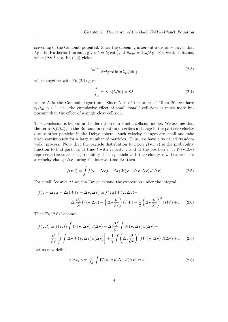
screening of the Coulomb potential. Since the screening is zero at a distance larger thatλD, the Rutherford formula gives b = b0 cot θ2 , at θmin = 2b0/λD. For weak collisions,when |∆v|2 ∼ v, Eq.(2.2) yields

tm '1

8πb20nv ln(πλD/4b0)(2.3)

which together with Eq.(2.1) gives

t1tm' 8 ln(λ/b0) = 8Λ (2.4)

where Λ is the Coulomb logarithm. Since Λ is of the order of 10 to 20, we havet1/tm >> 1, i.e. the cumulative effect of small “small” collisions is much more im-portant than the effect of a single close collision.

This conclusion is helpful in the derivation of a kinetic collision model. We assume thatthe term (∂f/∂t)c in the Boltzmann equation describes a change in the particle velocitydue to other particles in the Debye sphere. Such velocity changes are small and takeplace continuously for a large number of particles. Thus, we have a so called “randomwalk” process. Note that the particle distribution function f(v,r, t) is the probabilityfunction to find particles at time t with velocity v and at the position r. If W (v,∆v)represents the transition probability that a particle with the velocity v will experiencesa velocity change ∆v during the interval time ∆t, then

f(v,t) =

∫f(v−∆v,t−∆t)W (v−∆v,∆v) d(∆v) (2.5)

For small ∆v and ∆t we can Taylor expand the expression under the integral

f(v−∆v,t−∆t)W (v−∆v,∆v) ' f(v,t)W (v,∆v)−

∆t∂f

∂tW (v,∆v)−

(∆v

∂

∂v

)(fW ) +

1

2

(∆v

∂

∂v

)2

(fW ) + ... (2.6)

Then Eq.(2.5) becomes

f(v, t) ' f(v, t)

∫W (v,∆v) d(∆v)−∆t

∂f

∂t

∫W (v,∆v) d(∆v)−

∂

∂v

[f

∫∆vW (v,∆v) d(∆v)

]+

1

2

∫ (∆v

∂

∂v

)2

fW (v,∆v) d(∆v) + ... (2.7)

Let us now define

< ∆vi >≡1

∆t

∫W (v,∆v)∆vi d(∆v) ≡ ai (2.8)

4


and

< ∆vi∆vj >≡1

∆t

∫W (v,∆v)∆vi∆vj d(∆v) ≡ bij (2.9)

Since W is normalized according to∫W (v,∆v) d(∆v) = 1 (2.10)

we obtain

(∂f

∂t)c = − ∂

∂vi(aif) +

1

2

∂2

∂vi∂vj(bijf) (2.11)

which is the Fokker-Planck collision model. In the literature Eq.(2.11) is often rewrittenby introducing

Ai = ai −1

2

∂bij∂vj

(2.12)

Dij =1

2bij (2.13)

where Ai is the friction coefficient and Dij is the diffusion coefficient in velocity space.The determination of these coeficients in order to obtain the Fokker-Planck operatordescribing the Coulumb collisions follows closely Ref. [34].

Our present discussion will concern the Fokker-Planck collision model for high-energyalpha particles produced by the thermonuclear D-T reactions. We assume that thebackground plasma consists of electrons and 50-50% D-T ions and that their distribu-tion functions are isotropic and Maxwellian. The plasma is assumed to be free fromimpurities and neutrals. The macroscopic electric field giving rise to a plasma potentialfield, as well as the direct alpha particle drift losses, are here neglected. In these condi-tions, the behaviour of the distribution function of the alpha particles can be describedby the equation, cf. [33].

∂fα∂t

= − 1

τs

1

v2∂

∂v

[v2(afα − d‖

∂fα∂v

)]+

1

r

∂

∂r

(rDα

∂fα∂r

)+

S04πv2α

δ(v − vα) (2.14)

where

a = −∑∗

4π(eαe∗)2n∗L

mαm∗v2Φ1

( vv∗

)(2.15)

and

d‖ =∑∗

2π(eαe∗)2n∗L

m2αv

Φ1(vv∗ )

( vv∗ )2

(2.16)

5


here

v∗ =

(2T ∗

m∗

)2

(2.17)

Φ(x) =2√π

∫ x

0e−ξ

2dξ (2.18)

Φ1(x) = Φ(x)− xdΦ

dx(2.19)

The coefficient a is associated to the slowing down (or friction) process, whereas thecoefficient d‖ is related to the diffusion in the velocity space. Both mechanisms areproduced due to the collisions between the alpha particles and the background plasma.The source term in Eq.(2.14) represents the density of alpha particles created per sec-ond through thermonuclear reactions. Since each thermonuclear reaction produces alphaparticles with almost mono-energetic and isotropic velocity distribution, the source termis approximated by being proportional to the delta function at v = vα. Note, thatS0 = ni/τf , where ni is the density of background ions and τf = 4/(ni < σv >) is thecharacteristic time of alpha particle generation as a result of the thermonuclear reactions.

Since the object of the study is the high-energy alpha particle population, some sim-plifications can be applied in order to achieve simpler relations.

Because v/ve << 1, we have

Φ1(v/ve) '4

3√π

(v

ve

)3

(2.20)

Φ(v/ve)−Φ1(v/ve)

2(v/ve)2' 4

3√π

v

ve(2.21)

For ions instead, we have v/vi >> 1, which gives

Φ1(v/vi) ' 1 (2.22)

Φ(v/vi)−Φ1(v/vi)

2(v/vi)2' 1 (2.23)

Thus the friction coefficient a can be written as

a = ae + ai (2.24)

where

ae = − vτs

(2.25)

here τs is the Spitzer slowing down time given by

τs =3mαmev

3e

16√πZ2

αe4neL

(2.26)

6


and

ai = − v3cτsv2

(2.27)

with vc being the critical velocity at which the background electrons and ions contributeequally to the slowing down of the alpha particles. That is

v3c =3√π

4v3eme

ne

∑i

Z2i nimi

≡ 3√π

4v3eme

ne[Z] (2.28)

The parallel diffusion coefficients are given by

d‖e =1

τs

mev2e

2mα(2.29)

d‖i =1

τs

miv2i v

3c

2mαv3(2.30)

Thus, we conclude that ∣∣∣∣aeai∣∣∣∣ ∼ ∣∣∣∣v3v3c

∣∣∣∣ ≥ 1 (2.31)∣∣∣∣d‖ed‖i∣∣∣∣ ∼ ∣∣∣∣v3v3c

∣∣∣∣ ≥ 1 (2.32)

and ∣∣∣∣d‖e/vae

∣∣∣∣ ∼ ∣∣∣∣ TeEα∣∣∣∣ << 1 (2.33)

where Eα = 3.5MeV . This means that for the velocity range vc ≤ v ≤ vα, wherevα =

√2Eα/mα, the difussion term can be neglected and the basic equation for high-

energy alpha particles becomes

∂fα∂t

=1

τs

1

v2∂

∂v[(v3 + v3c )fα] +

1

r

∂

∂r

(rDα

∂fα∂r

)+

S04πv2α

δ(v − vα) (2.34)

7

3General Solution for theFokker-Planck Equation

This chapter shows the steps followed toward the achievement of the general solutionfor the Fokker-Planck equation. At the end of the chapter, besides the general case, twosimplified cases are also presented in order to have a better insight into the behave ofthe distribution function.

Let us consider the Fokker-Planck equation in the presence of spatial diffusion

∂fα∂t

=1

τs(t)

1

v2∂

∂v[(v3 + v3c )fα] +

1

r

∂

∂r

(rDα(r,v)

∂fα∂r

)+S0(r,t)

4πv2αδ(v − vα) (3.1)

where we assume that Dα(r,v) = d(v)rk. Introducing

F = fα(v3 + v3c ) (3.2)

Eq.(3.1) becomes

∂F

∂t=v3 + v3cτs(t)v2

∂F

∂v+d(v)

r

∂

∂r

(rk+1∂F

∂r

)+S0(r,t)(v

3α + v3c )

4πv2αδ(v − vα) (3.3)

From the characteristics of Eq.(3.3), we have

v2dv

v3 + v3c= − dt

τs(t)(3.4)

which implies the choice of the variable transformationz =(v3+v3cv3α+v

3c

)exp

[3∫ t0

dt′

τs(t)

]τ = t

(3.5)

8

Chapter 3 General Solution for the Fokker-Planck Equation

Then, the derivatives in the new variables are obtained applying the chain rule

∂

∂t=

∂

∂τ

∂τ

∂t+

∂

∂z

∂z

∂t=

∂

∂τ+

3

τs(t)z∂

∂z(3.6)

and

∂

∂v=

∂

∂z

∂z

∂v=

∂

∂z

3v2

v3α + v3cexp

[3

∫ t

0

dt′

τs(t)

](3.7)

which gives∂F

∂τ=d(v)

r

∂

∂r

(rk+1∂F

∂r

)+S0(r,t)(v

3α + v3c )

4πv2αδ(v − vα) (3.8)

where

v =

[z(v3α + v3c ) exp

[−3

∫ τ

0

dt

τs(t)

]− v3c

] 13

(3.9)

Eq.(3.8) can be written as a initial value problem noticing that at

v = vα → z∗ = exp

[3

∫ τ∗

0

dt

τs(t)

](3.10)

i.e.

exp

[3

(∫ τ∗

τ

dt

τs(t)

)]=v3 + v3cv3α + v3c

(3.11)

so that atτ∗ = τ → v = vα (3.12)

and since∣∣∣∣∂v∂τ∣∣∣∣v=vα

=

∣∣∣∣ z3v2 (v3α + v3c )−3

τs(τ)exp

[−3

∫ τ

0

dt

τs(t)

]∣∣∣∣ =

=

∣∣∣∣∣ 1

τs(τ∗)v2αz∗(v3α + v3c ) exp

[−3

∫ τ∗

0

dt

τs(t)

]∣∣∣∣∣v=vα

=v3α + v3cτs(τ∗)v2α

(3.13)

We have

∂F

∂τ=d(z,τ)

r

∂

∂r(rk+1∂F

∂r) (3.14)

F (r,τ∗) =S0(r,τ

∗)(v3α + v3c )

4πv2α

∣∣∣∣∂τ∂v∣∣∣∣v=vα

=S0(r,τ

∗)τs(τ∗)

4π(3.15)

In Eq.(3.14) we separate the variables by introducing

F (r,τ) = R(r)T (τ) (3.16)

9


Then1

d(z, τ)T (τ)

dT

dτ=

1

R(r)r

d

dr

(rk+1∂R

∂r

)= −λ (3.17)

i.e.

dT

dτ+ λd(z,τ)T = 0 (3.18)

and

1

r

d

dr

(rk+1dR

dr

)+ λR = 0 (3.19)

The solution of Eq.(3.18) is

T (τ) = C1 exp

[−λ∫ τ

τ∗d(z,τ ′) dτ ′

](3.20)

while Eq.(3.19) takes the form

rkd2R

dr2+ (k + 1)rk−1

dR

dr+ λR = 0 (3.21)

Let us consider Eq. (3.21) by substituting

R = rαy(x); x = arβ (3.22)

This impliesdR

dr= αrα−1y + aβrα+β−1

dy

dx(3.23)

d2R

dr2= α(α− 1)rα−2y + αaβrα+β−2

dy

dx+ αβ(α+ β − 1)rα+β−2

dy

dx+

+ a2β2rα+2β−2 dy2

dx2(3.24)

Thus, Eq.(3.21) becomes

a2β2r2βd2y

dx2+ aβ(2α+ β + k)rβ

dy

dx+ [λr2−k + α(α+ k)]y = 0 (3.25)

Since x = arβ, it is obtained

β2x2d2y

dx2+ β(2α+ β + k)x

dy

dx+

[λ(xa

) 2−kβ

+ α(α+ k)

]y = 0 (3.26)

Imposing 2α+β+k

β = 1

2−kβ = 2

λβ2 = a

2−kβ

(3.27)

10


gives α = −k/2

β = 2−k2

a =√λ|β|

(3.28)

Consequently, Eq.(3.18) becomes a Bessel equation of order ν with

x2d2y

dx2+ x

dy

dx+ (x2 − µ2)y = 0 (3.29)

R = r−k/2y(x); x =2√λ

2− kr

2−k2 (3.30)

ν =k

2− k(3.31)

where k 6= 2 to avoid singularities in the order of the Bessel equation. The solution ofEq.(3.29) is

y(x) = C2Jν(x) = C2J k2−k

(γj(r)) (3.32)

where

γj(r) =2

2− k√λjr

2−k2 (3.33)

the Bessel function of second kind has not been considered for being singular at r =0. The total solution of Eq.(3.1) should obey, besides being bounded ∀r ∈ [0,r0], theboundary conditions

fα = 0 if

v > vα

v < vf (t)

r = r0

(3.34)

where

vf (t) = 3

√(v3α + v3c ) exp

[−3

∫ t

0

dt′

τs(t′)

]− v3c (3.35)

and represents the velocity front of the velocity distribution function evolving towardthermal energies. Then, the solution should be proportional to

H(vα − v)−H(vf (t)− v) (3.36)

where H(x) is a step function defined by

H(x) =

1 if x ≥ 0

0 if x < 0(3.37)

11


On the other hand, the boundary conditions impose

J k2−k

(γj(r0)) = 0 (3.38)

that is

λj = µ2jν(2− k)2

4rk−20 (3.39)

where µjν is the jth root of the bessel function of ν = kk−2 order, J k

k−2(µjν) = 0. The

total solution can be written as

fα(v,r,t) =H(vα − v)−H(vf (t)− v)

v3 + v3c

∞∑j=1

Cjr−k/2J k

2−k(γj(r))

exp

[−λj

∫ τ

τ∗d(z,τ ′) dτ ′

](3.40)

where ∫ τ

τ∗d(z,τ ′) dτ ′ = −τs

∫ v

vα

d(v′)v′2

v′3 + v3cdv′ (3.41)

i.e.

fα(v,r,t) =H(vα − v)−H(vf (t)− v)

v3 + v3c

∞∑j=1

Cjr−k/2J k

2−k(γj(r))

exp

[λjτs(t)

∫ v

vα

d(v′)v′2

v′3 + v3cdv′]

(3.42)

In order to satisfy the initial condition (3.15) we take the solution for F (z,τ) at τ = τ∗

and using the orthogonality properties of the Bessel function, obtain the relation

∞∑j=1

∫ r0

0r1−k/2J k

2−k(γj(r))

S0(r,τ∗)τs(τ

∗)

4πdr =

=∞∑j=1

∞∑i=1

∫ r0

0r1−kJ k

2−k(γj(r))J k

2−k(γi(r))Cjδij dr =

=

∞∑j=1

Cj

∫ r0

0r1−kJ2

k2−k

(γj(r)) dr (3.43)

which gives

Cj =

∫ r00

S0(r,τ∗)τs(τ∗)4π r

2−k2 J k

2−k(γj(r)) dr∫ r0

0 r1−kJ2k

2−k(γj(r)) dr

(3.44)

12

3.1 Case Dα = 0 Chapter 3 General Solution for the Fokker-Planck Equation

Thus, Eq. (3.42) becomes

fα(v,r,t) = [H(vα − v)−H(vf (t)− v)]τs(τ

∗)

4π(v3 + v3c )

∞∑j=1

J k2−k

(γj(r))r−k/2

exp

[λjτs(t)

∫ v

vα

d(v′)v′2

v′3 + v3cdv′] ∫ r0

0 S0(r,τ∗)r

2−k2 J k


0 r1−kJ2k

2−k(γj(r)) dr

(3.45)

It should be taken into account that the distribution function given by Eq.(3.45) onlyrepresents the high-energy part of the alpha particle distribution. To this solution shouldbe added a low energy thermal Maxwellian distribution representing the accumulatingalpha particle ashes. Furthermore, this solution is only valid for k < 2. In the casek > 2, the function J k

2−k(γj(r))r

−k/2 is singular at r = 0, i.e. the solution is unbounded

at r=0.

In order to have a better insight into the general solution (3.45), some specific simplifiedcases can be considered.

3.1 Case Dα = 0

In absence of spatial diffusion i.e. when Dα = 0, it can be found from (3.45) that


∗)S0(r,τ∗)

4π(v3 + v3c )(3.46)

where τ∗ is determined by ∫ τ∗

τ

dt

τs(t)=

1

3ln

(v3 + v3cv3α + v3c

)(3.47)

Equations (3.46) and (3.47) represent the well-known slowing-down solution [33].

3.2 Case Dα = const.

In this case, the solution (3.45) simplifies into


∗)

4π(v3 + v3c )∞∑j=1

J0(r√λj)∫ r00 S0(r,τ

∗)J0(r√λj)r dr∫ r0

0 J20 (r√λj)r dr

(v3 + v3cv3α + v3c

)Dατsλj/3(3.48)

13

3.2 Case Dα = const. Chapter 3 General Solution for the Fokker-Planck Equation

Figure 3.1: Qualitative graphic of the evolution in time of the alpha particle distribu-tion function. All the particles are born with the same velocity, but the friction with thebackground plasma slows down their energy.

where λj are determined by J0(r0√λj) = 0. The time-dependancy of the distribution

function (3.48) consists of a velocity front at

vf (t) = 3

√(v3α + v3c ) exp

[−3

∫ t

0

dt′

τs(t)

]− v3c (3.49)

Sliding along the steady-state solution towards thermal energies, cf. Figure 3.1 . As-suming for example, τs = 370ms and vα/vc = 3.2 gives that v = 0 after t = 430ms.

14

4Analysis of the Inversion

Condition

As it has been pointed out in the introduction, the occurence of the velocity-spacethermonuclear instabilities is that the alpha particles velocity distribution function isinverted in some part of the velocity space, i.e. ∂fα/∂v > 0. In this situation free energyis available to drive instabilities. Starting from the Fokker-Planck equation describingthe slowing-down of energetic alpha particles in the absence of spatial diffusion, thecriterion for determining whether the inversion of the alpha particle function occurs hasbeen derived in Refs.[30,31] and independently [32]. In a simplified form this criterionmay be written as

d lnS0dTi

dT i

dt+d

dtln(nT 3/2

e ) >3

τs(4.1)

which can directly be derived from Eq.(3.45). In physical terms, Eq.(4.1) states thatif the source S0, (or the electron temperature Te) is increased too rapidly, inversionoccurs. Since changes in S0 are often predominantly due to changes in the ion tem-perature Ti, Eq.(4.1) can be used to obtain a limit on the rate at which the tempera-ture must be increased to become inverted. It is convenient to demonstrate the abovecondition by assuming Te = Ti = T and introduce the critical heating rate, Tcr, de-termined by ∂fα/∂v = 0. The dependence of Tcr on T for differnt values of the pa-rameter η = (n/n)/(T /T ) is shown in Figure 4.1 taking n = 1014cm−3 and expectingT < 10KeV/s in the case of plasma heating by neutral injection (NBI) or RF waves, itcan be concluded from Figure 4.1 that the planned heating of large tokamaks will notgenerated inverted alpha particle distribution functions (and hence cannot drive ther-monuclear velocity space instabilities).

Let us now examine the possibility of the occurance of such instabilities in the presenceof spatial diffusion losses of alpha particles. In order to determine the inversion condition

15

Chapter 4 Analysis of the Inversion Condition

Figure 4.1: Critical plasma heating as a function of temperature

for the distribution function, fα, we use the obtained solution (3.45), to differentiate fαwith respect to v and obtain

∂fα∂v

=1

4πrk/2

∞∑j=1

J k2−k

(γj(r)) exp

[λjτs(t)

∫ v

vα

d(v′)v′2

v′3 + v3cdv′]

1

τs

∂τs∂τ∗

+ λjd(v) + λj∂τs∂τ∗

∫ v

vα

d(v′)v′2

v′3 + v3cdv′ +

∫ r00

∂S0∂τ∗ r

2−k2 J k


0 S0(r,τ∗)r1−kJ2k

2−k(γj(r)) dr

∫ r00 S0(r, τ

∗)r2−k2 J k


0 r1−kJ2k

2−k(γj(r)) dr

τs(τ∗)v2

(v3 + v3c )2

(4.2)

The inversion condition ∂fα∂v > 0 is fulfilled when

∂

∂tln

[∫ r0

0S0(r,τ

∗)r1−kJ2k

2−k(γ1(r)) dr

]+∂

∂tln τs >

3

τs−

− λ1d(v)

[1− ∂τs

∂t

1

d(v)

∫ vα

vd(v′)

v′2

v′3 + v3cdv′]

(4.3)

16


Figure 4.2: Representation of the velocity distribution function for ITER-like parameters(τs = 0.37s, r0 = 2.2m,Eα = 3.5MeV, vα/vc = 3.2, r = 0.1m,S0 = 2.65 1018s−1, k = 0).Considering that d3 < d2 < d1 note that the inversion occurs for higher velocities as wedecrease the value of d

The above equation represents the generalized condition for the instability due to thetime varying particle distribution function. In the equilibrium, when S0 and τs are bothconstant in time the condition (4.3) simply reduces to

λ1d(v) >3

τs(4.4)

where λ1 = minλj . Thus, the steady state alpha particle distribution function will beinverted in velocity space due to spatial diffusion if the criterion is satisfied. Of course,any finite heating rate will only increase the degree of inversion. It also follows fromEq.(4.4) that in case of a velocity dependance diffusion coeficient, i.e. d(v) = d0v

p, theinversion occurs only for

v > p

√3

λmd0τs(4.5)

and the distribution function looks like in Figure 4.2 or Figure 4.3 depending on whichparameter we are changing. The analysis shows that it is necessary to know explicitly

17


Figure 4.3: Representation of the velocity distribution function for ITER-like parameters(τs = 0.37s, r0 = 2.2m,Eα = 3.5MeV, vα/vc = 3.2, r = 0.1m,S0 = 2.65 1018s−1, d0 = 7) fordifferent values of k

the diffusion coefficient in order to determine the inversion conditions. This rely onthe knowledge of the physical mechanism behind the considered alpha particle diffusionprocess. For example, in the case of a constant diffusion coefficient (k = 0, p = 0), weobtain λm = 5.78/r20 and the condition for inversion becomes

Dα > 0.52r20τs

(4.6)

Assuming ITER-like parameters: r0 = 2.2, T = 15 keV, n = 2 · 1014 cm−3, we haveτs = 370ms and the necessary value of the diffusion coefficient to get inversion is Dα >6.8m2/s. Similarly, in the case when Dα = d0r

k(k = 1,p = 0), we find λm = 3.67/r0and the condition for inversion becomes

d0 > 0.82r0τs

(4.7)

which for the above parameters yields d0 > 4.9m/s. Another way of expressing theinversion criterion in the case of a velocity independent diffusion coefficient is to intro-duce an effective loss time, τL, in the Fokker-Planck equation. This can be done by

18


applying a formal averaging procedure, which reduces Eq.(3.1) to a velocity and timedependent problem for the averaged alpha particle distribution function. In order toaverage Eq.(3.2), an assumption about the profile of fα has to be made. A convenientmodel compatible with the boundary conditions is fα = fα0(1−r2/r20). Defining a formalaverage procedure as

A ≡ 2

r20

∫ r0

0rAdr (4.8)

and applying it to Eq.(3.1) yields

∂fα∂t

=χ

τs

1

v2∂

∂v[(v3 + v3c )fα]− fα

τL+

¯S0(r)

4πv2αδ(v − vα) (4.9)

where we have assumed the profiles T (r) = T0(1 − r2/r20)δ and n(r) = n0(1 − r2/r20)γ .Thus

χ =2(

2 + γ − 32δ) (

1 + 32δ − γ

) (4.10)

and the diffusion loss time is

τL =1

8d0rk−20

(4.11)

Assuming that for T > 10keV

< σv >' 1.5 · 1016T3/2i (m/s) (4.12)

When T is over 10 keV , the averaged value of S0 can be written as

S0 '1.5 · 10−16(1 + γ)2(1 + δ)3/2n2T 3/2(

1 + 32δ + 2γ

)4

(4.13)

The solution of Eq.(4.9) is given by

fα(v,t) =S0(τ

∗)τs(τ∗)

χ4π(v3α + v3c )exp

[−∫ t

τ∗dt′(

1

τL− 3χ

τs(t′)

)](4.14)

where τ∗ is determined by ∫ τ∗

τ

χ

τsdt′ =

1

3ln

(v3 + v3cv3α + v3c

)(4.15)

The inversion condition obtained directly from Eqs.(4.14) and (4.15) is

1

S0

∂S0∂t

+1

τs

∂τs∂t

>3χ

τs− 1

τL(4.16)

Note that this condition is equivalent with the result obtained in Refs. [30,31,32], whereτL has been introduced in a heuristic way by replacing the effect of the diffusion operatorin Eq.(3.1) by the diffusion loss time, i.e.

d0r

∂

∂r

(rk+1∂fα

∂r

)→ −fα

τL(4.17)

19


This shows that the steady state distribution is always inverted if

1

τL> 3

χ

τs(4.18)

Assuming for example δ = γ = 1/4 and k = 0, the condition (4.18) together withEqs.(4.10) and (4.11) give

Dα > 0.4r20τs0

(4.19)

where τs0 = τs(r = 0). This is in good agreement with the corresponding criterion(4.4). For finite heating rates we can assume that the time dependences of the plasmatemperature and density are

T = tν ; ne = tµ (4.20)

Then the general condition for inversion (4.16) predicts that inversion will be possiblefor heating times satisfying

t <

(3ν + µ

3χ/τs− 1

6τL

)−1(4.21)

For example for ν = 2, µ = 0 and δ = γ = 1/4 the velocity inversion of fα is possible for

t <

(15

8τs0− 1

6τL

)−1(4.22)

Note that large diffusion loss times, represent small values of spatial diffusion. Then,Eq.(4.22) expresses qualitately that the smaller the spatial diffusion is, the smaller theheating time must be in order to satisfy the inversion condition.

20

5Conclusions

The derived inversion condition, shows that the change in the slope of the velocity distri-bution function for high energy alpha particle, and consequently the posible emergenceof wave instabilities, can be achieved either by fast variations of temperature, the pres-ence of anomalous spatial diffusion or both effects at the same time.

In previous research regarding also the inversion criterion, where the effect of anomalousspatial diffusion was not included, the conclusions were that the inversion of the velocitydistribution function is only achievable through fast variations of temperature that arecompletely out of the scope of the present plasma heating systems. Therefore, the posiblewave instabilities excited by the studied mechanism are not a factor to take into account.

However, the conclusion of the present master thesis is that the posibility of inversion inthe velocity distribution function cannot be rejected because, besides the effects of fastvariations of temperature, the presence of spatial diffusions has to be considered. Evenin the steady-state case, large enough values of Dα can cause the inversion.

Finally, it has been left for further research, the derivation of an explicit function forDα, allowing the comparison of the values of Dα that satisfy the inverison conditionwith the experimental values, and the quantitatively assessment of the implications ofthe anomalous spatial diffusion in the system.

21

Bibliography

[1] A. B. Mikhajlovskii, in Problems of Plasma Physics (Edited by M. A. Leontivoch),Vol.9, Moscow (1979).

[2] D. Pfirsh, in Theory of Magnetically Confined Plasmas, Pergamon Press, Oxfordand New York (1979).

[3] Y. I. Kolesnichenko, Nuclear Fusion 20 (1980) 727.

[4] A. B. Mikhajlovskii, in Physics of Plasma in Thermonuclear Regimes (Edited byB. Coppi and W. Sadowskij), U. S. Department of energy (1981)

[5] M. Lisak, Physica Scripta 29 (1984) 87.

[6] L. V. Korablev, Sov. Phys. - JETP 26 (1968) 922.

[7] T. D. Kaladze, A. B. Mikhajlovskii, Sov. J. Plasma Phys. 1 (1975) 128 PhysicaScripta 29 (1984) 87.

[8] T. D. Kaladze, D. G. Lominadze, A. B. Mikhajlovskii, A. B. Pokhotelov, NuclearFusion 16 (1976) 465.

[9] T. D. Kaladze, A. B. Mikhajlovskii, Nuclear Fusion 17 (1977) 729.

[10] D. G. Lominadze, A. B. Mikhajlovskii, Sov. J. Plasma Physics 1 (1975) 291.

[11] T. D. Kaladze,Sov. J. Plasma Physics 7 (1981) 451.

[12] A. B. Mikhajlovskii,T. D. Kaladze, D. G. Lominadze, L. V. Tsamalashvili,Sov. J. Plasma Physics 5 (1979) 173.

[13] W. Sutton, D. J. Sigmar, G. H. Miley, Fusion Techn. 7 (1985) 374.

[14] T. D. Kaladze,Physica Scripta T16 (1987) 27.

[15] V. S. Belikov, Y. I. Kolesnichenko, V. I. Oraevskij, Sov. Phys. JETP 39 (1974) 828.

22

BIBLIOGRAPHY

[16] C. O. Beasley, A. B. Mikhajlovskii,D. G. Lominadze, Sov. J. Plasma Physics 2(1976) 95.

[17] T. D. Kaladze, A. B. Mikhajlovskii, Nuclear Fusion 17 (1977) 411.

[18] V. S. Belikov, Y. I. Kolesnichenko, A. B. Mikhajlovskii, V. A. Yavorskii,Sov. J. Plasma Physics 3 (1977) 146.

[19] D. J Sigmar, H. C. Chan, Nuclear Fusion 18 (1978) 1569.

[20] A. B. Mikhajlovskii, Sov. Physics - JETP 41 (1975) 890.

[21] A. B. Mikhajlovskii, A. L. Frenkel, Sov. J. Plasma Phys. 3 (1977) 677.

[22] M. N. Rosenbluth, P. H. Rutherford, Phys. Rev. Lett. 34 (1975) 1428.

[23] K. T. Tsang, D. J. Sigmar, J. C. Whitson, Phys. Fluids 24 (1981), 1508.

[24] Y. M. Li, S. M. Mahajan, D. W. Ross, Phys. Fluids 30 (1987) 1466.

[25] M. Bornatici, F. Engelmann, Quasilinear Transport of Alpha Particles in a TokamakPlasma, FOM Institute for Plasma Physics, Rijnhuizen, Nieuwegein, the Nether-lands, Res. Rep. PP. 79/04 (1979).

[26] V. S. Belikov, Y. I. Kolesnichenko, Nuclear Fusion 20 (1980) 1153.

[27] V. S. Belikov, Y. I. Kolesnichenko, A. D. Fursa, in Plasma Physics and ControlledNuclear Fusion Research (Proc. 7th Int. Conf. Innsbruck, 1978) Vol. 1, IAEA, Vi-enna (1979) 561

[28] D. Anderson, M. Lisak, Phys. Fluids 27 (1984) 925.

[29] M. Lisak, D. Anderson, H. Hamnen, Phys. Fluids 26 (1983) 3308.

[30] Y. I. Kolesnichenko, Sov. J. Plasma Phys. 6 (1980) 531.

[31] V. S. Belikov, Y. I. Kolesnichenko, V. A. Yavorskij, Nucl. Fusion 21 (1981) 1311.

[32] J. G. Cordey, R. J. Goldston, D. R. Mikkelsen, Nucl. Fusion 2 (1981) 581.

[33] D. V. Sivukhin in Reviews of Plasma Physics, edited by M. Leontovich, Vol.4 (1963).

[34] John Wesson, Tokamaks, International series of monographs on Physics 18, OxfordScience Publications (2004).

23

Documents

Fast Alpha Particle Distribution in the Presence of ...publications.lib.chalmers.se/records/fulltext/165105.pdfD is the Debye length and n is the plasma density, due to the Coulomb