FASCINATE: Fast Cross-Layer Dependency Inference onMulti-layered Networks

Chen Chen†, Hanghang Tong†, Lei Xie‡, Lei Ying†, and Qing He§†Arizona State University, {chen_chen, hanghang.tong, lei.ying.2}@asu.edu

‡City University of New York, lei.xie@hunter.cuny.edu§University at Buffalo, qinghe@buffalo.edu

ABSTRACTMulti-layered networks have recently emerged as a new networkmodel, which naturally finds itself in many high-impact applica-tion domains, ranging from critical inter-dependent infrastructurenetworks, biological systems, organization-level collaborations, tocross-platform e-commerce, etc. Cross-layer dependency, whichdescribes the dependencies or the associations between nodes acrossdifferent layers/networks, often plays a central role in many datamining tasks on such multi-layered networks. Yet, it remains adaunting task to accurately know the cross-layer dependency a prior.In this paper, we address the problem of inferring the missing cross-layer dependencies on multi-layered networks. The key idea behindour method is to view it as a collective collaborative filtering prob-lem. By formulating the problem into a regularized optimizationmodel, we propose an effective algorithm to find the local optimawith linear complexity. Furthermore, we derive an online algo-rithm to accommodate newly arrived nodes, whose complexity isjust linear wrt the size of the neighborhood of the new node. Weperform extensive empirical evaluations to demonstrate the effec-tiveness and the efficiency of the proposed methods.

1. INTRODUCTIONIn an increasingly connected world, networks from many high-

impact areas are often collected from multiple inter-dependent do-mains, leading to the emergence of multi-layered networks [4, 9,26, 29, 30]. A typical example of multi-layered networks is inter-dependent critical infrastructure network. As illustrated in Figure 1,the full functioning of the telecom network, the transportation net-work and the gas pipeline network is dependent on the power sup-ply from the power grid. While for the gas-fired and coal-firedgenerators in the power grid, their functioning is fully dependenton the gas and coal supply from the transportation network and thegas pipeline network. Moreover, to keep the whole complex sys-tem working in order, extensive communications are needed acrossthe networks, which are in turn supported by the telecom network.Another example is biological system, where the protein-proteininteraction network (PPI/gene network) is naturally linked to thedisease similarity network by the known disease-gene associations,

Permission to make digital or hard copies of all or part of this work for personal orclassroom use is granted without fee provided that copies are not made or distributedfor profit or commercial advantage and that copies bear this notice and the full cita-tion on the first page. Copyrights for components of this work owned by others thanACM must be honored. Abstracting with credit is permitted. To copy otherwise, or re-publish, to post on servers or to redistribute to lists, requires prior specific permissionand/or a fee. Request permissions from permissions@acm.org.

KDD ’16, August 13-17, 2016, San Francisco, CA, USAc© 2016 ACM. ISBN 978-1-4503-4232-2/16/08. . . $15.00

DOI: http://dx.doi.org/10.1145/2939672.2939784

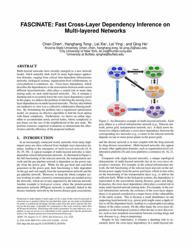
Figure 1: An illustrative example of multi-layered networks. Eachgray ellipse is a critical infrastructure network (e.g., Telecom net-work, power grid, transportation network, etc). A thick arrow be-tween two ellipses indicates a cross-layer dependency between thecorresponding two networks (e.g., a router in the telecom networkdepends on one or more power plants in the power grid).

and the disease network is in turn coupled with the drug networkby drug-disease associations. Multi-layered networks also appearin many other application domains, such as organization-level col-laboration platform [5] and cross-platform e-commerce [6, 16, 21,36].

Compared with single-layered networks, a unique topologicalcharacteristic of multi-layered networks lies in its cross-layer de-pendency structure. For example, in the critical infrastructure net-work, the full functioning of the telecom layer depends on the suf-ficient power supply from the power grid layer, which in turn relieson the functioning of the transportation layer (e.g., to deliver thesufficient fuel). While in the biological systems, the dependency isrepresented as the associations among diseases, genes and drugs.In practice, the cross-layer dependency often plays a central role inmany multi-layered network mining tasks. For example, in the crit-ical infrastructure network, the existence of the cross-layer depen-dency is in general considered as a major factor of the vulnerabilityof the entire system. This is because a small disturbance on onesupporting layer/network (e.g., power grid) might cause a ripple ef-fect to all the dependent layers, leading to a catastrophic/cascadingfailure of the entire system. On the other hand, the cross-layer de-pendency in the biological system is often the key to new discover-ies, such as new treatment associations between existing drugs andnew diseases (e.g., drug re-purposing).

Despite its key importance, it remains a daunting task to ac-curately know the cross-layer dependency in a multi-layered net-

work, due to a number of reasons, ranging from noise, incompletedata sources, limited accessibility to network dynamics. For ex-ample, an extreme weather event might significantly disrupt thepower grid, the transportation network and the cross-layer depen-dencies in between at the epicenter. Yet, due to limited accessibilityto the damage area during or soon after the disruption, the cross-layer dependency structure might only have a probabilistic and/orcoarse-grained description. On the other hand, for a newly identi-fied chemical in the biological system, its cross-layer dependencieswrt proteins and/or the diseases might be completely unknown dueto clinical limitations.(i.e., the zero-start problem).

In this paper, we aim to tackle the above challenges and developeffective and efficient methods to infer cross-layer dependency onmulti-layered networks. The main contributions of the paper canbe summarized as

• Problem Formulations. We formally formulate the cross-layer dependency inference problem as a regularized opti-mization problem. The key idea of our formulation is to col-lectively leverage the within-layer topology as well as theobserved cross-layer dependency to infer a latent, low-rankrepresentation for each layer, based on which the missingcross-layer dependencies can be inferred.

• Algorithms and Analysis. We propose an effective algorithm(FASCINATE) for cross-layer dependency inference on multi-layered networks, and analyze its optimality, convergenceand complexity. We further present its variants and gener-alizations, including an online algorithm to address the zero-start problem.

• Evaluations. We perform extensive experiments on real data-sets to validate the effectiveness, efficiency and scalability ofthe proposed algorithms. Specially, our experimental eval-uations show that the proposed algorithms outperform theirbest competitors by 8.2%-41.9% in terms of inference accu-racy while enjoying linear complexity. Specifically, the pro-posed FASCINATE-ZERO algorithm can achieve up to 107×speedup with barely no compromise on accuracy.

The rest of the paper is organized as follows. Section 2 gives theformal definitions of the cross-layer dependency inference prob-lems. Section 3 proposes FASCINATE algorithm with its analysis.Section 4 introduces the zero-start algorithm FASCINATE-ZERO.Section 5 presents the experiment results. Section 6 reviews therelated works. Section 7 summarizes the paper.

2. PROBLEM DEFINITIONIn this section, we give the formal definitions of the cross-layer

dependency inference problems. The main symbols used through-out the paper are listed in Table 1. Following the convention, weuse bold upper-case for matrices (e.g., A), bold lower-case for vec-tors (e.g., a) and calligraphic for sets (e.g., A). A′ denotes thetranspose of matrix A. We use the ˆ sign to denote the notations

after a new node is accommodated to the system (e.g., J , A1), andthe ones without the ˆ sign as the notations before the new nodearrives.

While several multi-layered network models exist in the litera-ture (See Section 6 for a review), we will focus on a recent modelproposed in [5], due to its flexibility to model more complicatedcross-layer dependency structure. We refer the readers to [5] forits full details. For the purpose of this paper, we mainly need thefollowing notations to describe a multi-layered network with g lay-ers. First, we need a g×g layer-layer dependency matrix G, where

Table 1: Main Symbols.

Symbol Definition and Description

A,B the adjacency matrices (bold upper case)a,b column vectors (bold lower case)A,B sets (calligraphic)

A(i, j) the element at ith row jth columnin matrix A

A(i, :) the ith row of matrix AA(:, j) the jth column of matrix AA′ transpose of matrix A

A the adjacency matrix of A with the newly added node

G the layer-layer dependency matrixA within-layer connectivity matrices of the network

A = {A1, . . . ,Ag}D cross-layer dependency matrices

D = {Di,j i, j = 1, ..., g}Wi,j weight matrix for Di,j

Fi low-rank representation for layer-i (i = 1, ..., g)mi, ni number of edges and nodes in graph Ai

mi,j number of dependencies in Di,j

g total number of layersr the rank for {Fi}i=1,...,g

t the maximal iteration numberξ the threshold to determine the iteration

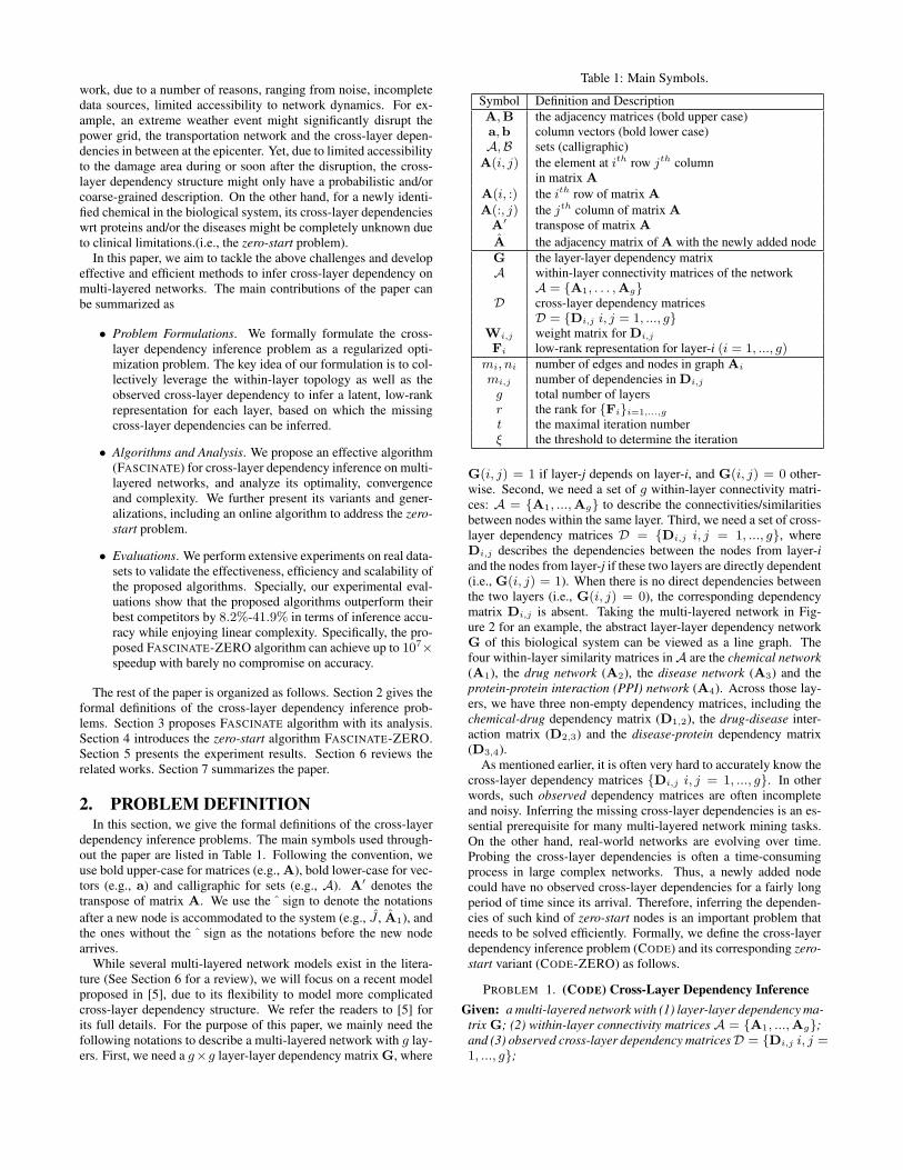
G(i, j) = 1 if layer-j depends on layer-i, and G(i, j) = 0 other-wise. Second, we need a set of g within-layer connectivity matri-ces: A = {A1, ...,Ag} to describe the connectivities/similaritiesbetween nodes within the same layer. Third, we need a set of cross-layer dependency matrices D = {Di,j i, j = 1, ..., g}, whereDi,j describes the dependencies between the nodes from layer-iand the nodes from layer-j if these two layers are directly dependent(i.e., G(i, j) = 1). When there is no direct dependencies betweenthe two layers (i.e., G(i, j) = 0), the corresponding dependencymatrix Di,j is absent. Taking the multi-layered network in Fig-ure 2 for an example, the abstract layer-layer dependency networkG of this biological system can be viewed as a line graph. Thefour within-layer similarity matrices inA are the chemical network(A1), the drug network (A2), the disease network (A3) and theprotein-protein interaction (PPI) network (A4). Across those lay-ers, we have three non-empty dependency matrices, including thechemical-drug dependency matrix (D1,2), the drug-disease inter-action matrix (D2,3) and the disease-protein dependency matrix(D3,4).

As mentioned earlier, it is often very hard to accurately know thecross-layer dependency matrices {Di,j i, j = 1, ..., g}. In otherwords, such observed dependency matrices are often incompleteand noisy. Inferring the missing cross-layer dependencies is an es-sential prerequisite for many multi-layered network mining tasks.On the other hand, real-world networks are evolving over time.Probing the cross-layer dependencies is often a time-consumingprocess in large complex networks. Thus, a newly added nodecould have no observed cross-layer dependencies for a fairly longperiod of time since its arrival. Therefore, inferring the dependen-cies of such kind of zero-start nodes is an important problem thatneeds to be solved efficiently. Formally, we define the cross-layerdependency inference problem (CODE) and its corresponding zero-start variant (CODE-ZERO) as follows.

PROBLEM 1. (CODE) Cross-Layer Dependency InferenceGiven: a multi-layered network with (1) layer-layer dependency ma-trix G; (2) within-layer connectivity matrices A = {A1, ...,Ag};and (3) observed cross-layer dependency matricesD = {Di,j i, j =1, ..., g};

Figure 2: A simplified 4-layered network for biological systems.

Output: the true cross-layer dependency matrices {Di,j i, j =1, ..., g} .

PROBLEM 2. (CODE-ZERO) Cross-Layer Dependency In-ference for zero-start Nodes

Given: (1) a multi-layered network {G,A,D}; (2) a newly addednode p in the lth layer; (3) a 1 × nl vector s that records the con-nections between p and the existing nl nodes in layer l;

Output: the true dependencies between node p and nodes in depen-dent layers of layer-l, i.e., Dl,j(p, :) (j = 1, ..., g, G(l, j) = 1).

3. FASCINATE FOR PROBLEM 1In this section, we present our proposed solution for Problem 1

(CODE). We start with the proposed optimization formulation, andthen present our algorithm (FASCINATE), followed by some effec-tiveness and efficiency analysis.

3.1 FASCINATE: Optimization FormulationThe key idea behind our formulation is to treat Problem 1 as

a collective collaborative filtering problem. To be specific, if weview (1) nodes from a given layer (e.g., power plants) as objectsfrom a given domain (e.g., users/items), (2) the within-layer con-nectivity (e.g., communication networks) as an object-object sim-ilarity measure, and (3) the cross-layer dependency (e.g., depen-dencies between computers in the communication layer and powerplants in power grid layer) as the ‘ratings’ from objects of one do-main to those of another domain; then inferring the missing cross-layer dependencies can be viewed as a task of inferring the miss-ing ratings between the objects (e.g., users, items) across differentdomains. Having this analogy in mind, we propose to formulateProblem 1 as the following regularized optimization problem

minFi≥0(i=1,...,g)

J =∑

i,j: G(i,j)=1

‖Wi,j � (Di,j − FiFj′)‖2F

︸ ︷︷ ︸C1: Matching Observed Cross-Layer Dependencies

(1)

+ α

g∑i=1

tr(Fi′(Ti −Ai)Fi)︸ ︷︷ ︸

C2: Node Homophily

+β

g∑i=1

‖Fi‖2F︸ ︷︷ ︸C3: Regularization

where Ti is the diagonal degree matrix of Ai with Ti(u, u) =∑niv=1 Ai(u, v); Wi,j is an ni × nj weight matrix to assign dif-

ferent weights to different entries in the corresponding cross-layerdependency matrix Di,j ; and Fi is the low-rank representation forlayer i. For now, we set the weight matrices as follows: Wi,j(u, v)= 1 if Di,j(u, v) is observed, and Wi,j(u, v) ∈ [0, 1] if Di,j(u, v)= 0 (i.e., unobserved). To simplify the computation, we set theweights of all unobserved entries to a global value w. We will dis-cuss alternative choices for the weight matrices in Section 3.3.

In this formulation (Eq. (1)), we can think of Fi as the low-rankrepresentations/features of the nodes in layer i in some latent space,which is shared among different layers. The cross-layer dependen-cies between the nodes from two dependent layers can be viewedas the inner product of their latent features. Therefore, the intuitionof the first term (i.e. C1) is that we want to match all the cross-layer dependencies, calibrated by the weight matrix Wi,j . Thesecond term (i.e., C2) is used to achieve node homophily, whichsays that for a pair of nodes u and v from the same layer (saylayer-i), their low-rank representations should be similar (i.e., small‖Fi(u, :) − Fi(v, :)‖2) if the within-layer connectivity betweenthese two nodes is strong (i.e., large Ai(u, v)). The third term (i.e.C3) is to regularize the norm of the low-rank matrices {Fi}i=1,...,g

to prevent over-fitting.Once we solve Eq. (1), for a given node u from layer-i and a

node v from layer-j, the cross-layer dependency between them canbe estimated as Di,j(u, v) = Fi(u, :)Fj(v, :)

′.

3.2 FASCINATE: Optimization AlgorithmThe optimization problem defined in Eq. (1) is non-convex. Thus,

we seek to find a local optima by the block coordinate descentmethod, where each Fi naturally forms a ‘block’. To be specific,if we fix all other Fj(j = 1, . . . , g, j �= i) and ignore the constantterms, Eq. (1) can be simplified as

JiFi≥0

=∑

j: G(i,j)=1

‖Wi,j � (Di,j − FiFj′)‖2F (2)

+ αtr(Fi′(Ti −Ai)Fi) + β‖Fi‖2F

The derivative of Ji wrt Fi is

∂Ji

∂Fi=2(

∑j: G(i,j)=1

[−(Wi,j �Wi,j �Di,j)Fj (3)

+ (Wi,j �Wi,j � (FiFj′))Fj ]

+ αTiFi − αAiFi + βFi)

A fixed-point solution of Eq. (3) with non-negativity constrainton Fi leads to the following multiplicative updating rule for Fi

Fi(u, v)← Fi(u, v)

√X(u, v)

Y(u, v)(4)

where

X =∑

j: G(i,j)=1

(Wi,j �Wi,j �Di,j)Fj + αAiFi (5)

Y =∑

j: G(i,j)=1

(Wi,j �Wi,j � (FiFj′))Fj + αTiFi + βFi

Recall that we set Wi,j(u, v) = 1 when Di,j(u, v) > 0, andWi,j(u, v) = w when Di,j(u, v) = 0. Here, we define IOi,jas an indicator matrix for the observed entries in Di,j , that is,IOi,j(u, v) = 1 if Di,j(u, v) > 0, and IOi,j(u, v) = 0 if Di,j(u, v) =0. Then, the estimated dependencies over the observed data can berepresented as Ri,j = IOi,j� (FiFj). With these notations, we can

further simplify the update rule in Eq. (5) as follows

X =∑

j: G(i,j)=1

Di,jFj + αAiFi (6)

Y =∑

j: G(i,j)=1

((1− w2)Ri,j + w2FiFj′)Fj + αTiFi + βFi

(7)

The proposed FASCINATE algorithm is summarized in Alg. 1.First, it randomly initializes the low-rank matrices for each layer(line 1 - line 3). Then, it begins the iterative update procedure.In each iteration (line 4 - line 10), the algorithm alternatively up-dates {Fi}i=1,...,g one by one. We use two criteria to terminatethe iteration: (1) either the Frobenius norm between two successiveiterations for all {Fi}i=1,...,g is less than a threshold ξ, or (2) themaximum iteration number t is reached.

Algorithm 1 The FASCINATE Algorithm

Input: (1) a multi-layered network with (a) layer-layer depen-dency matrix G, (b) within-layer connectivity matrices A ={A1, ...,Ag}, and (c) observed cross-layer node dependencymatrices D = {Di,j i, j = 1, ..., g}; (2) the rank size r; (3)weight w; (4) regularized parameters α and β;

Output: low-rank representations for each layer {Fi}i=1,...,g

1: for i = 1 to g do2: initialized Fi as ni × r non-negative random matrix3: end for4: while not converge do5: for i = 1 to g do6: compute X as Eq. (6)7: compute Y as Eq. (7)8: update Fi as Eq. (4)9: end for

10: end while11: return {Fi}i=1,...,g

3.3 Proof and AnalysisHere, we analyze the proposed FASCINATE algorithm in terms

of its effectiveness as well as its efficiency.

A - Effectiveness Analysis.In terms of effectiveness, we show that the proposed FASCINATE

algorithm indeed finds a local optimal solution to Eq. (1). To seethis, we first give the following theorem, which says that the fixedpoint solution of Eq. (4) satisfies the KKT condition.

THEOREM 1. The fixed point solution of Eq. (4) satisfies theKKT condition.

PROOF. The Lagrangian function of Eq. (2) can be written as

Li =∑

j: G(i,j)=1

‖Wi,j � (Di,j − FiFj′)‖2F (8)

+ αtr(Fi′TiFi)− αtr(Fi

′AiFi) + β‖Fi‖2F − tr(Λ′Fi)

where Λ is the Lagrange multiplier. Setting the derivative of Li wrtFi to 0, we get

2(∑

j: G(i,j)=1

[−(Wi,j �Wi,j �Di,j)Fj (9)

+ (Wi,j �Wi,j � (FiFj′))Fj ]

+ αTiFi − αAiFi + βFi) = Λ

By the KKT complementary slackness condition, we have

[∑

j: G(i,j)=1

(Wi,j �Wi,j � (FiFj′))Fj + αTiFi + βFi

︸ ︷︷ ︸Y

(10)

− (∑

j: G(i,j)=1

(Wi,j �Wi,j �Di,j)Fj + αAiFi)

︸ ︷︷ ︸X

](u, v)Fi(u, v) = 0

Therefore, we can see that the fixed point solution of Eq. (4) satis-fies the above equation.

The convergence of the proposed FASCINATE algorithm is givenby the following lemma.

LEMMA 1. Under the updating rule in Eq. (4), the objectivefunction in Eq. (2) decreases monotonically.

PROOF. Omitted for brevity.

According to Theorem 1 and Lemma 1, we conclude that Alg. 1converges to a local minimum solution for Eq. 2 wrt each individualFi.

B - Efficiency Analysis.In terms of efficiency, we analyze both the time complexity as

well as the space complexity of the proposed FASCINATE algo-rithm, which are summarized in Lemma 2 and Lemma 3. We cansee that FASCINATE scales linearly wrt the size of the entire multi-layered network.

LEMMA 2. The time complexity of Alg. 1 is O([g∑

i=1

(∑

j: G(i,j)=1

(mi,jr + (ni + nj)r2) +mir)]t).

PROOF. In each iteration in Alg. 1 for updating Fi, the com-plexity of calculating X by Eq. (6) is O(

∑j: G(i,j)=1

mi,jr +mir)

due to the sparsity of Di,j and Ai. The complexity of computing

Ri,j in Y is O(mi,jr). Computing Fi(F′jFj) requires O((ni +

nj)r2) operations and computing αTiFi + βFi requires O(nir)

operations. So, it is of O(∑

j: G(i,j)=1

(mi,jr + (ni + nj)r2)) com-

plexity to get Y in line 7. Therefore, it takes O(∑

j: G(i,j)=1

(mi,jr+

(ni + nj)r2) +mir) to update Fi. Putting all together, the com-

plexity of updating all low-rank matrices in each iteration is O(g∑

i=1

(∑

j: G(i,j)=1

(mi,jr + (ni + nj)r2) + mir)). Thus, the overall

complexity of Alg. 1 is O([g∑

i=1

(∑

G(i,j)=1

(mi,jr + (ni + nj)r2) +

mir)]t), where t is the maximum number of iterations in the algo-rithm.

LEMMA 3. The space complexity of Alg. 1 is O(∑g

i=1(nir +mi) +

∑i,j: G(i,j)=1

mi,j) .

PROOF. It takes O(∑g

i=1 nir) to store all the low-rank matri-ces, and O(

∑gi=1 mi +

∑i,j: G(i,j)=1

mi,j) to store all the within-

layer connectivity matrices and dependency matrices in the multi-layered network. To calculate X for Fi, it costs O(nir) to com-pute

∑j: G(i,j)=1

Di,jFj and αAiFi. For Y, the space cost of com-

puting Ri,j and Fi(F′jFj) is O(mi,j) and O(nir) respectively.

Therefore, the space complexity of calculating∑

j: G(i,j)=1

((1 −

w2)Ri,j + w2FiFj′)Fj is O( max

j: G(i,j)=1mi,j + nir). On the

other hand, the space required to compute αTiFi+βFi is O(nir).Putting all together, the space cost of updating all low-rank matri-ces in each iteration is of O( max

i,j: G(i,j)=1mi,j +maxi nir). Thus,

the overall space complexity of Alg. 1 is O(∑g

i=1(nir + mi) +∑i,j: G(i,j)=1

mi,j).

C - Variants.Here, we discuss some variants of the proposed FASCINATE al-

gorithm. First, by setting all the entries in the weight matrix Wi,j

to 1, FASCINATE becomes a clustering algorithm (i.e., Fi can beviewed as the cluster membership matrix for nodes in layer-i). Fur-thermore, if we restrict ourselves to two-layered networks (i.e.,g = 2), FASCINATE becomes a dual regularized co-clustering algo-rithm [20]. Second, by setting w ∈ (0, 1), FASCINATE can be usedto address one class collaborative filtering problem, where implicitdependencies extensively exist between nodes from different lay-ers. Specifically, on two-layered networks, FASCINATE is reducedto a weighting-based, dual-regularized one class collaborative fil-tering algorithm [37]. Third, when the within-layer connectivitymatricesA = {A1, . . . ,Ag} are absent, the proposed FASCINATE

can be viewed as a collective matrix factorization method [32].While the proposed FASCINATE includes these existing methods

as its special cases, its major advantage lies in its ability to collec-tively leverage all the available information (e.g., the within-layerconnectivity, the observed cross-layer dependency) for dependencyinference. As we will demonstrate in the experimental section, sucha methodical strategy leads to a substantial and consistent inferenceperformance boosting. Nevertheless, a largely unanswered ques-tion for these methods (including FASCINATE) is how to handlezero-start nodes. That is, when a new node arrives with no ob-served cross-layer dependencies, how can we effectively and effi-ciently infer its dependencies without rerunning the algorithm fromscratch. In the next section, we present a sub-linear algorithm tosolve this problem (i.e., Problem 2).

4. FASCINATE-ZERO FOR PROBLEM 2A multi-layered network often exhibits high dynamics, e.g., the

arrival of new nodes. For example, for a newly identified chemicalin the biological system, we might know how it interacts with someexisting chemicals (i.e., the within-layer connectivity). However,its cross-layer dependencies wrt proteins and/or diseases might becompletely unknown . This section addresses such zero-start prob-lems (i.e., Problem 2). Without loss of generality, we assume thatthe newly added node resides in layer-1, indexed as its (n1 + 1)th

node. The within-layer connectivity between the newly added nodeand the existing n1 nodes is represented by a 1× n1 row vector s,where s(u) (u = 1, ..., n1) denotes the (within-layer) connectivitybetween the newly added node and the uth existing node in layer-1.

We could just rerun our FASCINATE algorithm on the entire multi-layered network with the newly added node to get its low-rank rep-resentation (i.e., a 1 × r row vector f ), based on which its cross-layer dependencies can be estimated. However, the running timeof this strategy is linear wrt the size of the entire multi-layerednetwork. For example, on a three-layered infrastructure networkwhose size is in the order of 14 million, it would take FASCINATE

2, 500+ seconds to update the low-rank matrices {Fi} for a zero-start node with rank r = 200, which might be too costly in onlinesettings. In contrast, our upcoming algorithm is sub-linear, and it

only takes less than 0.001 seconds on the same network withoutjeopardizing the accuracy.

There are two key ideas behind our online algorithm. The firstis to view the newly added node as a perturbation to the originalnetwork. In detail, the updated within-layer connectivity matrix

A1 for layer-1 can be expressed as

A1 =

[A1 s′

s 0

](11)

where A1 is the within-layer connectivity matrix for layer-1 beforethe arrival of the new node.

Correspondingly, the updated low-rank representation matrix for

layer-1 can be expressed as F1 = [F′1(n1×r) f ′]′, where F1(n1×r)

is the updated low-rank representation for the existing n1 nodes

in layer-1. Then the new objective function J in Eq. (1) can bereformatted as

J =∑

i,j: G(i,j)=1i,j �=1

‖Wi,j � (Di,j − FiF′j)‖2F (12)

+∑

j: G(1,j)=1

‖W1,j � (D1,j − F1F′j)‖2F

+

g∑i=2

α

2

ni∑u=1

ni∑v=1

Ai(u, v)‖Fi(u, :)− Fi(v, :)‖22

+α

2

n1∑u=1

n1∑v=1

A1(u, v)‖F1(u, :)− F1(v, :)‖22

+ β

g∑i=2

‖Fi‖2F + β‖F′1(n1×r)‖2F

+ α

n1∑v=1

s(v)‖f − F1(v, :)‖22 + β‖f‖22

Since the newly added node has no dependencies, we can set

W1,j =

[W(1,j)

0(1×nj)

], D1,j =

[D(1,j)

0(1×nj)

]Therefore, the second term in J can be simplified as∑

j: G(1,j)=1

‖W1,j � (D1,j − F1(n1×r)F′j)‖2F (13)

Combining Eq. (12), Eq. (13) and J in Eq. (1) together, J can beexpressed as

J = J + J1(14)

where J1 = α∑n1

v=1 s(v)‖f − F1(v, :)‖22 + β‖f‖22, and J is theobjective function without the newly arrived node.

The second key idea of our online algorithm is that in Eq. (14),J is often orders of magnitude larger than J1. For example, in theBIO dataset used in Section 5.2.2, J is in the order of 103, whileJ1 is in the order of 10−1. This naturally leads to the following ap-proximation strategy, that is, we (1) fix J with {F∗

i }i=1,...,g (i.e.,the previous local optimal solution to Eq. (1) without the newlyarrived node), and (2) optimize J1 to find out the low-rank repre-sentation f for the newly arrived node. That is, we seek to solve thefollowing optimization problem

f = argminf≥0

J1subject to: F1(n1×r) = F∗

1 (15)

with which, we can get an approximate solution {Fi}i=1,...,g to J .

To solve f , we take the derivative of J1 wrt f and get

1

2

∂J1

∂f= βf + α

n1∑v=1

s(v)(f − F∗1(v, :)) (16)

= (β + α

n1∑v=1

s(v))f − αsF∗1

Since α and β are positive, the Hessian matrix of J1 is a positivediagonal matrix. Therefore, the global minimum of J1 can be ob-tained by setting its derivative to zero. Then the optimal solution toJ1 can be expressed as

f =αsF∗

1

β + α∑n1

v=1 s(v)(17)

For the newly added node, f can be viewed as the weighted averageof its neighbors’ low-rank representations. Notice that in Eq. (17),the non-negativity constraint on f naturally holds. Therefore, werefer to this solution (i.e., Eq. (17)) as FASCINATE-ZERO. In thisway, we can successfully decouple the cross-layer dependency in-ference problem for zero-start node from the entire multi-layerednetwork and localize it only among its neighbors in layer-1. Thelocalization significantly reduces the time complexity, as summa-rized in Lemma 4, which is linear wrt the number of neighbors ofthe new node (and therefore is sub-linear wrt the size of the entirenetwork).

LEMMA 4. Let nnz(s) denotes the total number of within-layerlinks between the newly added node and the original nodes in layer-1 (i.e., nnz(s) is the degree for the newly added node). Then thetime complexity of FASCINATE-ZERO is O(nnz(s)r).

PROOF. Since the links between the newly added node and theoriginal nodes in layer-1 are often very sparse, the number of non-zero elements in s (nnz(s)) is much smaller than n1. Therefore,the complexity of computing sF∗

1 can be reduced to O(nnz(s)r).The multiplication between α and sF∗

1 takes O(r). Computing∑n1v=1 s(v) takes O(nnz(s)). Thus, the overall complexity of com-

puting f is O(nnz(s)r).

5. EVALUATIONSIn this section, we evaluate the proposed FASCINATE algorithms.

All experiments are designed to answer the following questions:

• Effectiveness. How effective are the proposed FASCINATE

algorithms in inferring the missing cross-layer dependencies?

• Efficiency. How fast and scalable are the proposed algo-rithms?

5.1 Experimental Setup

5.1.1 Datasets DescriptionWe perform our evaluations on four different datasets, including

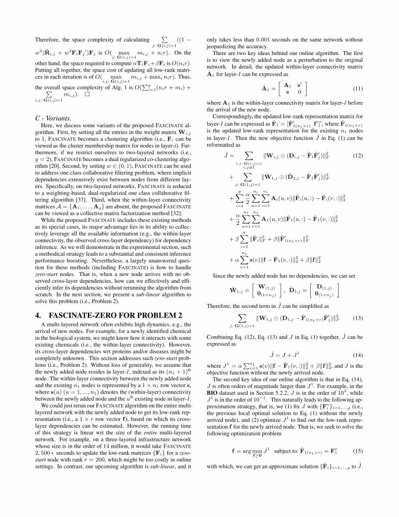
(1) a three-layer Aminer academic network in the social collabora-tion domain (SOCIAL); (2) a three-layer CTD (Comparative Tox-icogenomics Database) network in the biological domain (BIO);(3) a five-layer Italy network in the critical infrastructure domain(INFRA-5); and (4) a three-layer network in the critical infrastruc-ture domain (INFRA-3). The statistics of these datasets are shownin Table 2, and the abstract layer-layer dependency graphs of thesefour datasets are summarized in Figure 3. In all these four data-sets, the cross-layer dependencies are binary and undirected (i.e.,Di,j(u, v) = Dj,i(v, u)).

Table 2: Statistics of Datasets.

Dataset # of Layers # of Nodes # of Links # of CrossLinksSOCIAL 3 125,344 214,181 188,844

BIO 3 35,631 253,827 75,456INFRA-5 5 349 379 565INFRA-3 3 15,126 29,861 28,023,500

(a) SOCIAL (b) BIO (c) INFRA-5 (d) INFRA-3

Figure 3: The abstract dependency structure of each dataset.

SOCIAL. This dataset contains three layers, including a col-laboration network among authors, a citation network between pa-pers and a venue network [33]. The number of nodes in each layerranges from 899 to 62, 602, and the number of within-layer linksranges from 2, 407 to 201, 037. The abstract layer-layer depen-dency graph of SOCIAL is shown in Figure 3(a). The collab-oration layer is connected to the paper layer with the authorshipdependency, while the venue layer is connected to the paper layerwith publishing dependency. For the Paper-Author dependency,we have 126,242 links cross the two layers; for the Paper-Venuedependency, we have 62,602 links.

BIO. The construction of CTD network is based on the worksin [7, 27, 34]. It contains three layers, which are chemical, dis-ease and gene similarity networks. The number of nodes in thesenetworks ranges from 4, 256 to 25, 349, and the number of within-layer links ranges from 30, 551 to 154, 167. The interactions be-tween chemicals, genes, and diseases form the cross-layer depen-dency network as shown in Figure 3(b). For Chemical-Gene de-pendency, we have 53,735 links cross the two layers; for Chemical-Disease dependency, we have 19,771 links; and for Gene-Diseasedependency, we have 1,950 links.

INFRA-5. The construction of this critical infrastructure net-work is based on the data implicated from an electrical blackoutin Italy in Sept 2003 [28]. It contains five layers, including fourlayers of regional power grids and one Internet network [28]. Theregional power grids are partitioned by macroregions1. To makethe regional networks more balanced, we merge the Southern Italypower grid and the Island power grid together. The power transferlines between the four regions are viewed as cross-layer dependen-cies. For the Italy Internet network, it is assumed that each Internetcenter is supported by the power stations within a radius of 70km.Its abstract dependency graph is shown in Figure 3(c). The small-est layer in the network has 39 nodes and 50 links; while the largestnetwork contains 151 nodes and 158 links. The number of depen-dencies is up to 307.

INFRA-3. This dataset contains the following three critical in-frastructure networks: an airport network2, an autonomous systemnetwork3 and a power grid [35]. We construct a three-layered net-work in the same way as [5]. The three infrastructure networksare functionally dependent on each other. Therefore, they forma triangle-shaped multi-layered network as shown in Figure 3(d).The construction of the cross-layer dependencies is based on geo-graphic proximity. The number of nodes in each layer varies from

1https://en.wikipedia.org/wiki/First-level_NUTS_of_the_European_Union2http://www.levmuchnik.net/Content/Networks/NetworkData.html3http://snap.stanford.edu/data/

2, 833 to 7, 325, and the number of within-layer links ranges from6, 594 to 15, 665. The number of cross-layer dependencies rangesfrom 4, 434, 116 to 14, 921, 765.

For all datasets, we randomly select 50% cross-layer dependen-cies as the training set and use the remaining 50% as the test set.

5.1.2 Comparing MethodsWe compare FASCINATE with the following methods, including

(1) FASCINATE-CLUST - a variant of the proposed method for thepurpose of dependency clustering, (2) MulCol - a collective ma-trix factorization method [32], (3) PairSid - a pairwise one-classcollaborative filtering method proposed in [37], (4) PairCol - apairwise collective matrix factorization method degenerated fromMulCol (5) PairNMF - a pairwise non-negative matrix factoriza-tion (NMF) based method [19], (6) PairRec - a pairwise matrixfactorization based algorithm introduced in [15], (7) FlatNMF -an NMF based method that treats the input multi-layered networkas a flat-structured single network (i.e., by putting the within-layerconnectivity matrices in the diagonal blocks, and the cross-layerdependency matrices in the off-diagonal blocks), and (8) FlatRec- a matrix factorization based method using the same techniquesas PairRec but treating the input multi-layered network as a singlenetwork as in FlatNMF.

For the experimental results reported in this paper, we set rankr = 100, maximum iteration t = 100, termination threshold ξ =10−8, weight w2 = 0.1 and regularization parameters α = 0.1,β = 0.1 unless otherwise stated.

5.1.3 Evaluation MetricsWe use the following metrics for the effectiveness evaluations.

• MAP. It measures the mean average precision over all enti-ties in the cross-layer dependency matrices [18]. A largerMAP indicates better inference performance.

• R-MPR. It is a variant of Mean Percentage Ranking for one-class collaborative filtering [12]. MPR is originally used tomeasure the user’s satisfaction of items in a ranked list. Inour case, we can view the nodes from one layer as users,and the nodes of the dependent layer(s) as items. The rankedlist therefore can be viewed as ordered dependencies by theirimportance. Smaller MPR indicates better inference perfor-mance. Specifically, for a randomly produced list, its MPR isexpected to be 50%. Here, we define R-MPR = 0.5−MPR,so that larger R-MRP indicates better inference performance.

• HLU. Half-Life Utility is also a metric from one-class col-laborative filtering. By assuming that the user will view eachconsecutive items in the list with exponential decay of possi-bility, it estimates how likely a user will choose an item froma ranked list [25]. In our case, it measures how likely a nodewill establish dependencies with the nodes in the ranked list.A larger HLU indicates better inference performance.

• AUC. Area Under ROC Curve is a metric that measures theclassification accuracy. A larger AUC indicates better infer-ence performance.

• Prec@K. Precision at K is defined by the proportion of truedependencies among the top K inferred dependencies. Alarger Prec@K indicates better inference performance.

5.1.4 Machine and RepeatabilityAll the experiments are performed on a machine with 2 proces-

sors Intel Xeon 3.5GHz with 256GB of RAM. The algorithms are

programmed with MATLAB using single thread. We will releasethe code and the non-proprietary datasets after the paper is pub-lished.

5.2 EffectivenessIn this section, we aim to answer the following three questions,

(1) how effective is FASCINATE for Problem 1 (i.e., CODE)? (2)how effective is FASCINATE-ZERO for Problem 2 (i.e., CODE-ZERO)? and (3) how sensitive are the proposed algorithms wrt themodel parameters?

5.2.1 Effectiveness of FASCINATE

We compare the proposed algorithms and the existing methodson all the four datasets. The results are shown in Table 3 throughTable 6. There are several interesting observations. First is thatour proposed FASCINATE algorithm and its variant (FASCINATE-CLUST) consistently outperform all other methods in terms of allthe five evaluation metrics. Second, by exploiting the structure ofmulti-layered network, FASCINATE, FASCINATE-CLUST and Mul-Col have significantly better performance than the pairwise meth-ods. Third, among the pairwise baselines, PairSid and PairCol arebetter than PairNMF and PairRec. The main reason is that the firsttwo algorithms utilize both within-layer connectivity matrices andcross-layer dependency matrix for matrix factorization, while thelatter two only use the observed dependency matrix. Finally, therelatively poor performance of FlatNMF and FlatRec implies thatsimply flattening the multi-layered network into a single networkis insufficient to capture the intrinsic correlations across differentlayers.

We also test the sensitivity of the proposed algorithms wrt thesparsity of the observed cross-layer dependency matrices (i.e., theratio of the missing values) on INFRA-3. The results in Fig-ure 4 demonstrate that both FASCINATE and FASCINATE-CLUST

perform well even when 90%+ entries in the dependency matricesare missing.

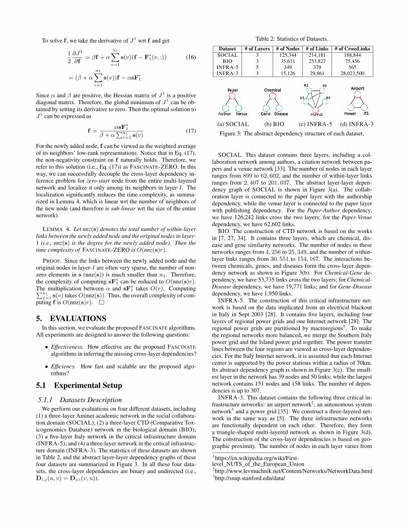
5.2.2 Effectiveness of FASCINATE-ZERO

To evaluate the effectiveness of FASCINATE-ZERO, we randomlyselect one node from the Chemical layer in the BIO dataset as thenewly arrived node and compare the inference performance be-tween FASCINATE-ZERO and FASCINATE. The average resultsover multiple runs are presented in Figure 5. We can see thatFASCINATE-ZERO bears a very similar inference power as FAS-CINATE, but it is orders of magnitude faster. We observe similarperformance when the zero-start nodes are selected from the othertwo layers (i.e., Gene and Disease).

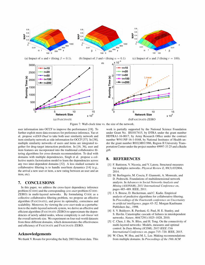
5.2.3 Parameter StudiesThere are three parameters α, β and r in the proposed FASCI-

NATE algorithm. α is used to control the impact of node homophily,β is used to avoid over-fitting, and r is the number of columns of thelow-rank matrices {Fi}. We fix one of these parameters, and studythe impact of the remaining two on the inference results. From Fig-ure 6, we can see that MAP is stable over a wide range of both αand β. Specifically, a relatively high MAP can be achieved when αis between 0.1 to 1 and β is less than 1. As for the third parameter r,the inference performance quickly increases wrt r until it hits 200,after which the MAP is almost flat. This suggests that a relativelysmall size of the low-rank matrices might be sufficient to achieve asatisfactory inference performance.

5.3 EfficiencyThe scalability results of FASCINATE and FASCINATE-ZERO

are presented in Figure 7. As we can see in Figure 7(a), FASCI-

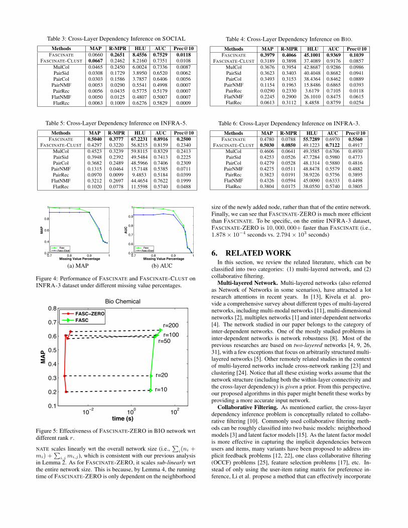
Table 3: Cross-Layer Dependency Inference on SOCIAL

Methods MAP R-MPR HLU AUC Prec@10FASCINATE 0.0660 0.2651 8.4556 0.7529 0.0118

FASCINATE-CLUST 0.0667 0.2462 8.2160 0.7351 0.0108

MulCol 0.0465 0.2450 6.0024 0.7336 0.0087PairSid 0.0308 0.1729 3.8950 0.6520 0.0062PairCol 0.0303 0.1586 3.7857 0.6406 0.0056

PairNMF 0.0053 0.0290 0.5541 0.4998 0.0007PairRec 0.0056 0.0435 0.5775 0.5179 0.0007

FlatNMF 0.0050 0.0125 0.4807 0.5007 0.0007FlatRec 0.0063 0.1009 0.6276 0.5829 0.0009

Table 4: Cross-Layer Dependency Inference on BIO.

Methods MAP R-MPR HLU AUC Prec@10FASCINATE 0.3979 0.4066 45.1001 0.9369 0.1039

FASCINATE-CLUST 0.3189 0.3898 37.4089 0.9176 0.0857

MulCol 0.3676 0.3954 42.8687 0.9286 0.0986PairSid 0.3623 0.3403 40.4048 0.8682 0.0941PairCol 0.3493 0.3153 38.4364 0.8462 0.0889

PairNMF 0.1154 0.1963 15.8486 0.6865 0.0393PairRec 0.0290 0.2330 3.6179 0.7105 0.0118

FlatNMF 0.2245 0.2900 26.1010 0.8475 0.0615FlatRec 0.0613 0.3112 8.4858 0.8759 0.0254

Table 5: Cross-Layer Dependency Inference on INFRA-5.

Methods MAP R-MPR HLU AUC Prec@10FASCINATE 0.5040 0.3777 67.2231 0.8916 0.2500

FASCINATE-CLUST 0.4297 0.3220 56.8215 0.8159 0.2340

MulCol 0.4523 0.3239 59.8115 0.8329 0.2413PairSid 0.3948 0.2392 49.5484 0.7413 0.2225PairCol 0.3682 0.2489 48.5966 0.7406 0.2309

PairNMF 0.1315 0.0464 15.7148 0.5385 0.0711PairRec 0.0970 0.0099 9.4853 0.5184 0.0399

FlatNMF 0.3212 0.2697 44.4654 0.7622 0.1999FlatRec 0.1020 0.0778 11.5598 0.5740 0.0488

Table 6: Cross-Layer Dependency Inference on INFRA-3.

Methods MAP R-MPR HLU AUC Prec@10FASCINATE 0.4780 0.0788 55.7289 0.6970 0.5560

FASCINATE-CLUST 0.5030 0.0850 49.1223 0.7122 0.4917

MulCol 0.4606 0.0641 49.3585 0.6706 0.4930PairSid 0.4253 0.0526 47.7284 0.5980 0.4773PairCol 0.4279 0.0528 48.1314 0.5880 0.4816

PairNMF 0.4275 0.0511 48.8478 0.5579 0.4882PairRec 0.3823 0.0191 38.9226 0.5756 0.3895

FlatNMF 0.4326 0.0594 45.0090 0.6333 0.4498FlatRec 0.3804 0.0175 38.0550 0.5740 0.3805

0.7 0.8 0.9 10.2

0.4

0.6

0.8

1

Missing Value Percentage

MA

P

FascFasc−Clust

0.7 0.8 0.9 10.5

0.6

0.7

0.8

0.9

1

Missing Value Percentage

AU

C

FascFasc−Clust

(a) MAP (b) AUC

Figure 4: Performance of FASCINATE and FASCINATE-CLUST onINFRA-3 dataset under different missing value percentages.

10−2

100

102

0.1

0.2

0.3

0.4

0.5

0.6

0.7

0.8

time (s)

MA

P

Bio Chemical

FASC−ZEROFASC

r=20

r=10

r=200

r=50r=100

Figure 5: Effectiveness of FASCINATE-ZERO in BIO network wrtdifferent rank r.

NATE scales linearly wrt the overall network size (i.e.,∑

i(ni +mi) +

∑i,j mi,j), which is consistent with our previous analysis

in Lemma 2. As for FASCINATE-ZERO, it scales sub-linearly wrtthe entire network size. This is because, by Lemma 4, the runningtime of FASCINATE-ZERO is only dependent on the neighborhood

size of the newly added node, rather than that of the entire network.Finally, we can see that FASCINATE-ZERO is much more efficientthan FASCINATE. To be specific, on the entire INFRA-3 dataset,FASCINATE-ZERO is 10, 000, 000+ faster than FASCINATE (i.e.,1.878× 10−4 seconds vs. 2.794× 103 seconds)

6. RELATED WORKIn this section, we review the related literature, which can be

classified into two categories: (1) multi-layered network, and (2)collaborative filtering.

Multi-layered Network. Multi-layered networks (also referredas Network of Networks in some scenarios), have attracted a lotresearch attentions in recent years. In [13], Kivela et al. pro-vide a comprehensive survey about different types of multi-layerednetworks, including multi-modal networks [11], multi-dimensionalnetworks [2], multiplex networks [1] and inter-dependent networks[4]. The network studied in our paper belongs to the category ofinter-dependent networks. One of the mostly studied problems ininter-dependent networks is network robustness [8]. Most of theprevious researches are based on two-layered networks [4, 9, 26,31], with a few exceptions that focus on arbitrarily structured multi-layered networks [5]. Other remotely related studies in the contextof multi-layered networks include cross-network ranking [23] andclustering [24]. Notice that all these existing works assume that thenetwork structure (including both the within-layer connectivity andthe cross-layer dependency) is given a prior. From this perspective,our proposed algorithms in this paper might benefit these works byproviding a more accurate input network.

Collaborative Filtering. As mentioned earlier, the cross-layerdependency inference problem is conceptually related to collabo-rative filtering [10]. Commonly used collaborative filtering meth-ods can be roughly classified into two basic models: neighborhoodmodels [3] and latent factor models [15]. As the latent factor modelis more effective in capturing the implicit dependencies betweenusers and items, many variants have been proposed to address im-plicit feedback problems [12, 22], one class collaborative filtering(OCCF) problems [25], feature selection problems [17], etc. In-stead of only using the user-item rating matrix for preference in-ference, Li et al. propose a method that can effectively incorporate

0 0.01

1 100 0

200400

600800

10000

0.2

0.4

0.6

0.8

rα

MA

P

0 0.01

1 100 0

200400

600800

10000

0.2

0.4

0.6

0.8

rβ

MA

P

0

0.01

1

100

0

0.01

1

100

0

0.2

0.4

0.6

0.8

βα

MA

P

(a) Impact of α and r (fixing β = 0.1). (b) Impact of β and r (fixing α = 0.1) (c) Impact of α and β (fixing r = 100).

Figure 6: The parameter studies of the BIO dataset.

0 5 10 15

x 106

0

500

1000

1500

2000

2500

3000

Network Size

Ru

nn

ing

Tim

e (s

)

r=10r=20r=50r=100r=200

0 5 10 15

x 106

0

1

2

3

4x 10

−4

Network Size

Ru

nn

ing

Tim

e (s

)

r=10r=20r=50r=100r=200

Linear

(a) FASCINATE (b)FASCINATE-ZERO

Figure 7: Wall-clock time vs. the size of the network.

user information into OCCF to improve the performance [18]. Tofurther exploit more data resources for preference inference, Yao etal. propose wiZAN-Dual to take both user similarity network anditem similarity network as side information for OCCF [37]. In [38],multiple similarity networks of users and items are integrated to-gether for drug-target interaction prediction. In [16, 36], user anditem features are incorporated into the traditional collaborative fil-tering algorithms for cross-domain recommendation. To deal withdomains with multiple dependencies, Singh et al. propose a col-lective matrix factorization model to learn the dependencies acrossany two inter-dependent domains [32]. A less studied scenario incollaborative filtering is to handle user/item dynamics [14] (e.g.,the arrival a new user or item, a new rating between an user and anitem, etc).

7. CONCLUSIONSIn this paper, we address the cross-layer dependency inference

problem (CODE) and the corresponding zero-start problem (CODE-ZERO) in multi-layered networks. By formulating CODE as acollective collaborative filtering problem, we propose an effectivealgorithm (FASCINATE), and prove its optimality, correctness andscalability. Moreover, by viewing the zero-start node as a perturba-tion to the multi-layered network system, we derive an effective andefficient algorithm (FASCINATE-ZERO) to approximate the depen-dencies of newly added nodes, whose complexity is sub-linear wrtthe overall network size. We experiment on four real-world datasetsfrom three different domains, which demonstrates the effectivenessand efficiency of FASCINATE and FASCINATE-ZERO.

AcknowledgementsWe thank V. Rosato for providing the Italy 2003 blackout data. This

work is partially supported by the National Science Foundationunder Grant No. IIS1017415, by DTRA under the grant numberHDTRA1-16-0017, by Army Research Office under the contractnumber W911NF-16-1-0168, by National Institutes of Health un-der the grant number R01LM011986, Region II University Trans-portation Center under the project number 49997-33 25 and a Baidugift.

8. REFERENCES[1] F. Battiston, V. Nicosia, and V. Latora. Structural measures

for multiplex networks. Physical Review E, 89(3):032804,2014.

[2] M. Berlingerio, M. Coscia, F. Giannotti, A. Monreale, andD. Pedreschi. Foundations of multidimensional networkanalysis. In Advances in Social Networks Analysis andMining (ASONAM), 2011 International Conference on,pages 485–489. IEEE, 2011.

[3] J. S. Breese, D. Heckerman, and C. Kadie. Empiricalanalysis of predictive algorithms for collaborative filtering.In Proceedings of the Fourteenth conference on Uncertaintyin artificial intelligence, pages 43–52. Morgan KaufmannPublishers Inc., 1998.

[4] S. V. Buldyrev, R. Parshani, G. Paul, H. E. Stanley, andS. Havlin. Catastrophic cascade of failures in interdependentnetworks. Nature, 464(7291):1025–1028, 2010.

[5] C. Chen, J. He, N. Bliss, and H. Tong. On the connectivity ofmulti-layered networks: Models, measures and optimalcontrol. In Data Mining (ICDM), 2015 IEEE 15thInternational Conference on, pages 715–720. IEEE, 2015.

[6] W. Chen, W. Hsu, and M. L. Lee. Making recommendationsfrom multiple domains. In Proceedings of the 19th ACM

SIGKDD international conference on Knowledge discoveryand data mining, pages 892–900. ACM, 2013.

[7] A. P. Davis, C. J. Grondin, K. Lennon-Hopkins,C. Saraceni-Richards, D. Sciaky, B. L. King, T. C. Wiegers,and C. J. Mattingly. The comparative toxicogenomicsdatabase’s 10th year anniversary: update 2015. Nucleic acidsresearch, page gku935, 2014.

[8] J. Gao, S. V. Buldyrev, S. Havlin, and H. E. Stanley.Robustness of a network of networks. Physical ReviewLetters, 107(19):195701, 2011.

[9] J. Gao, S. V. Buldyrev, H. E. Stanley, and S. Havlin.Networks formed from interdependent networks. Naturephysics, 8(1):40–48, 2012.

[10] D. Goldberg, D. Nichols, B. M. Oki, and D. Terry. Usingcollaborative filtering to weave an information tapestry.Communications of the ACM, 35(12):61–70, 1992.

[11] L. S. Heath and A. A. Sioson. Multimodal networks:Structure and operations. Computational Biology andBioinformatics, IEEE/ACM Transactions on, 6(2):321–332,2009.

[12] Y. Hu, Y. Koren, and C. Volinsky. Collaborative filtering forimplicit feedback datasets. In Data Mining, 2008. ICDM’08.Eighth IEEE International Conference on, pages 263–272.Ieee, 2008.

[13] M. Kivelä, A. Arenas, M. Barthelemy, J. P. Gleeson,Y. Moreno, and M. A. Porter. Multilayer networks. Journalof Complex Networks, 2(3):203–271, 2014.

[14] Y. Koren. Collaborative filtering with temporal dynamics. InProceedings of the 15th ACM SIGKDD internationalconference on Knowledge discovery and data mining, pages447–456. ACM, 2009.

[15] Y. Koren, R. Bell, and C. Volinsky. Matrix factorizationtechniques for recommender systems. Computer, (8):30–37,2009.

[16] B. Li, Q. Yang, and X. Xue. Can movies and bookscollaborate? cross-domain collaborative filtering for sparsityreduction. In IJCAI, volume 9, pages 2052–2057, 2009.

[17] J. Li, X. Hu, L. Wu, and H. Liu. Robust unsupervised featureselection on networked data. In Proceedings of SIAMInternational Conference on Data Mining. SIAM, 2016.

[18] Y. Li, J. Hu, C. Zhai, and Y. Chen. Improving one-classcollaborative filtering by incorporating rich user information.In Proceedings of the 19th ACM international conference onInformation and knowledge management, pages 959–968.ACM, 2010.

[19] C.-b. Lin. Projected gradient methods for nonnegative matrixfactorization. Neural computation, 19(10):2756–2779, 2007.

[20] J. Liu, C. Wang, J. Gao, Q. Gu, C. C. Aggarwal, L. M.Kaplan, and J. Han. Gin: A clustering model for capturingdual heterogeneity in networked data. In SDM, pages388–396. SIAM, 2015.

[21] Z. Lu, W. Pan, E. W. Xiang, Q. Yang, L. Zhao, and E. Zhong.Selective transfer learning for cross domainrecommendation. In SDM, pages 641–649. SIAM, 2013.

[22] H. Ma. An experimental study on implicit socialrecommendation. In Proceedings of the 36th internationalACM SIGIR conference on Research and development ininformation retrieval, pages 73–82. ACM, 2013.

[23] J. Ni, H. Tong, W. Fan, and X. Zhang. Inside the atoms:ranking on a network of networks. In Proceedings of the 20thACM SIGKDD international conference on Knowledgediscovery and data mining, pages 1356–1365. ACM, 2014.

[24] J. Ni, H. Tong, W. Fan, and X. Zhang. Flexible and robustmulti-network clustering. In Proceedings of the 21th ACMSIGKDD International Conference on Knowledge Discoveryand Data Mining, pages 835–844. ACM, 2015.

[25] R. Pan, Y. Zhou, B. Cao, N. N. Liu, R. Lukose, M. Scholz,and Q. Yang. One-class collaborative filtering. In DataMining, 2008. ICDM’08. Eighth IEEE InternationalConference on, pages 502–511. IEEE, 2008.

[26] R. Parshani, S. V. Buldyrev, and S. Havlin. Interdependentnetworks: reducing the coupling strength leads to a changefrom a first to second order percolation transition. Physicalreview letters, 105(4):048701, 2010.

[27] S. Razick, G. Magklaras, and I. M. Donaldson. irefindex: aconsolidated protein interaction database with provenance.BMC bioinformatics, 9(1):1, 2008.

[28] V. Rosato, L. Issacharoff, F. Tiriticco, S. Meloni,S. Porcellinis, and R. Setola. Modelling interdependentinfrastructures using interacting dynamical models.International Journal of Critical Infrastructures,4(1-2):63–79, 2008.

[29] A. Sen, A. Mazumder, J. Banerjee, A. Das, and R. Compton.Multi-layered network using a new model ofinterdependency. arXiv preprint arXiv:1401.1783, 2014.

[30] J. Shao, S. V. Buldyrev, S. Havlin, and H. E. Stanley.Cascade of failures in coupled network systems withmultiple support-dependent relations. arXiv preprintarXiv:1011.0234, 2010.

[31] J. Shao, S. V. Buldyrev, S. Havlin, and H. E. Stanley.Cascade of failures in coupled network systems withmultiple support-dependence relations. Physical Review E,83(3):036116, 2011.

[32] A. P. Singh and G. J. Gordon. Relational learning viacollective matrix factorization. In Proceedings of the 14thACM SIGKDD international conference on Knowledgediscovery and data mining, pages 650–658. ACM, 2008.

[33] J. Tang, J. Zhang, L. Yao, J. Li, L. Zhang, and Z. Su.Arnetminer: extraction and mining of academic socialnetworks. In Proceedings of the 14th ACM SIGKDDinternational conference on Knowledge discovery and datamining, pages 990–998. ACM, 2008.

[34] M. A. Van Driel, J. Bruggeman, G. Vriend, H. G. Brunner,and J. A. Leunissen. A text-mining analysis of the humanphenome. European journal of human genetics,14(5):535–542, 2006.

[35] D. J. Watts and S. H. Strogatz. Collective dynamics ofsmall-world networks. nature, 393(6684):440–442, 1998.

[36] D. Yang, J. He, H. Qin, Y. Xiao, and W. Wang. Agraph-based recommendation across heterogeneous domains.In Proceedings of the 24rd ACM International Conference onConference on Information and Knowledge Management,pages 463–472. ACM, 2015.

[37] Y. Yao, H. Tong, G. Yan, F. Xu, X. Zhang, B. K. Szymanski,and J. Lu. Dual-regularized one-class collaborative filtering.In Proceedings of the 23rd ACM International Conference onConference on Information and Knowledge Management,pages 759–768. ACM, 2014.

[38] X. Zheng, H. Ding, H. Mamitsuka, and S. Zhu. Collaborativematrix factorization with multiple similarities for predictingdrug-target interactions. In Proceedings of the 19th ACMSIGKDD international conference on Knowledge discoveryand data mining. ACM, 2013.