University of HelsinkiDepartment of Economics and ManagementPublications No. 34, Production Economics andFarm ManagementHelsinki 2002

Sauli Sonkkila

Farmers’ decision-making on adjustmentinto the EU

Selostus: Maatilayrittäjien EU-sopeutumiseen liittyväpäätöksenteko

Academic dissertation

To be presented with the permission of the Faculty of Agriculture and Forestry ofthe University of Helsinki, for public examination in Sali 13, Fabianinkatu 33,University of Helsinki, on March 1th 2002, at 12:00 noon.

Helsingin yliopisto, Taloustieteen laitosJulkaisuja nro 34, Maatalouden liiketaloustiede

Helsingfors universitet, Institutionen för ekonomiPublikationer Nr 34, Lantbrukets företagsekonomi

Supervised by: Professor Matti YlätaloDepartment of Economics and ManagementUniversity of HelsinkiHelsinki, Finland

Reviewed by: Professor Bo ÖhlmerDepartment of EconomicsThe Swedish University of Agricultural SciencesUppsala, Sweden

Professor Emeritus Matti KeltikangasUniversity of HelsinkiHelsinki, Finland

Discussed with: Professor Pekka KorhonenDepartment of EconomyHelsinki School of Economics and Business AdministrationHelsinki, Finland

ISBN 952-10-0280-8 (nid.)ISBN 952-10-0281-6 (pdf)

ISSN 1235-2241

http://ethesis.helsinki.fi

To Sampsa and Loviisa

Preface

This study is the outcome of long labour. It is based on my licentiate dissertation onthe same subject. I express my thanks to all the people who helped me completethat work, and especially Professor Karl Johan Weckman, who helped me getstarted as a researcher.

I extend my warmest thanks to Professor Matti Ylätalo for the guidance, supportand encouragement he has given me during my four-year task. The support I havereceived from Dr Mikko Siitonen at different stages of my work deserves specialmention. His encouragement and assistance greatly helped me finish my work.

I thank the preliminary scrutineers, Professor Bo Öhlmer and Professor EmeritusMatti Keltikangas, for the expert advice that helped me bring my work to conclu-sion.

I thank all the farmers who participated in the study. It would not have beenpossible to complete my work without their input.

Kielitoimisto Habil edited the English text. I would like to thank them for theirgood work.

I thank the Finnish Cultural Foundation for their financial assistance. I also thankmy employer the Information Centre of the Ministry of Agriculture and Forestry forall its support while I was working on the study.

A “thank you” is also in order to my parents, Tuula and Matti Sonkkila, who havealways encouraged me in my studies and provided me with the opportunity toadvance in my academic career. My wife’s parents, Ulla and Markku Rytsölä, havealso always had an understanding attitude to my studies.

Moving back to my native Laitila to become a farmer at the beginning of 1999brought a new depth to my views and motivated me to take the study forward. Onthe other hand, it has forced me to reprioritise my work.

My children, Sampsa and Loviisa, have over the years grown accustomed to Daddyspending his time in the study when home. I thank them for putting up with me andfor the encouragement they have given me.

Last but not least, my wife Elina deserves my special thanks for all her support andunderstanding, which has helped me a great deal in my work.

Salo, LaitilaDecember 2001Sauli Sonkkila

Esipuhe

Tämä tutkimus on pitkän työrupeaman tulos. Työ pohjautuu lisensiaattityöhöni,joka käsitteli samaa aihealuetta kuin käsillä oleva työ. Kiitän kaikkia niitä, jotkatuolloin olivat edesauttamassa työni valmistumista. Erityisesti haluan mainitaprofessori Karl Johan Weckmanin, joka auttoi minua tutkijaurani alkumetreillä.

Pyydän esittää parhaat kiitokseni professori Matti Ylätalolle ohjauksesta, tuesta jakannustuksesta, jonka olen saanut neljän vuoden urakkani aikana. Erityisesti haluankiittää MMT Mikko Siitosta kannustuksesta työni eri vaiheissa. Mikon kannustus jaapu työn eri vaiheissa on suuresti auttanut minua viemään työni päätökseen.

Kiitän tutkimuksen esitarkastajia, professori Bo Öhlmeriä ja emeritus professoriMatti Keltikangasta asiantuntevista neuvoista, jotka auttoivat viemään työtänieteenpäin ja loppuunsaattamaan sen.

Kiitän kaikkia tutkimukseen osallistuneita maatilayrittäjiä. Ilman heidän panostaantutkimus ei olisi ollut mahdollinen.

Tekstin kielentarkistuksen on suorittanut Habil Oy. Haluan esittää heille kiitoksenhyvin tehdystä työstä.

Kiitän Suomen Kulttuurirahastoa saamastani taloudellisesta tuesta, joka on mah-dollistanut tutkimuksen toteuttamisen. Kiitän myös työnantajaani, Maa- ja metsä-talousministeriön tietopalvelukeskusta kaikesta tuesta, jota olen saanut tehdessänitutkimusta.

Kiitokset kuuluvat myös vanhemmilleni, Tuula ja Matti Sonkkilalle, jotka ovat jokouluajoista lähtien kannustaneet minua opiskelemaan ja antaneet mahdollisuudenetenemiseen akateemisella uralla. Myös vaimoni vanhemmat, Ulla ja MarkkuRytsölä, ovat aina suhtautuneet ymmärtäväisesti opiskeluuni.

Muuttaminen takaisin synnyinseudulleni Laitilaan ja ryhtyminen maatilayrittäjäksivuoden 1999 alussa on omalta osaltaan syventänyt näkemyksiäni ja motivoinuttutkimuksen eteenpäinviemisessä, vaikka toisaalta onkin pakottanut asettamaan työttärkeysjärjestykseen.

Lapseni, Sampsa ja Loviisa, ovat vuosien aikana saaneet tottua siihen, että kotonaollessaan isä sulkeutuu työhuoneeseensa tutkimaan. Kiitos myös teille jaksamisestaja tuesta.

Lopuksi haluan kiittää vaimoani Elinaa kaikesta tuesta ja ymmärryksestä, joka onollut tarpeen tämän työn tekemiseksi.

Laitilan Salon kylässäjoulukuussa 2001Sauli Sonkkila

University of HelsinkiDepartment of Economics and ManagementPublications No. 34, Production Economics and

Farm Management, 2002. 160 p.

Farmers’ decision-making on adjustment into the EU

Sauli Sonkkila

Abstract: This study aims at explaining farmers’ decision-making on adjustmentinto the EU, and examining changes in their objectives, values, attitudes towardrisk, managerial issues, and the significance of risk factors in the changing opera-tional environment.

The empirical data for the study consisted of three sets of data. A postal survey in1993 was conducted for active Finnish farmers with at least 10 hectares of arableland. In 1998, a follow-up survey was carried out for the same set of farmers whoresponded to the 1993 survey. These two data sets were complemented and vali-dated by the data received from the rural business register.

Almost half of the farmers had maintained current production, one fifth had ex-panded production and 15% had quit production. The tests indicated that theproduction and economic factors of the farm, characteristics of the farmer and theoperational environment affected decision-making on adjustment into the EU. Themagnitude and interaction of these factors seemed to vary from one farm andfarmer to another.

The most important objectives and values had remained same during the five-yearperiod. The most important objectives were those associated with risk managementand the most important values were intrinsic values. However, farmers’ objectivesand values had altered somewhat upon joining the EU compared with the timebefore membership. Values associated with entrepreneurship and the objective ofimproving the quality of products had been less prioritised, while objectives relatedto the quality of life and leisure as well as environmental issues had been prioritisedhigher in the operational environment of the EU. The major reason behind thesechanges was the introduction of the EU common agricultural policy (CAP), whichgreatly altered the farmers’ operational environment between 1993 and 1998.

Keywords: Risk, uncertainty, decision-making, objectives, values, farms,farmers, Finland, European Union

ISBN 952-10-0280-8 (nid.)ISBN 952-10-0281-6 (pdf)

ISSN 1235-2241

ContentsPage

1. Introduction ........................................................................................................... 9

1.1 Background of the study.................................................................................. 9

1.2 Objective of the study.................................................................................... 12

1.3 Methodological approach and research process ............................................ 13

2. Risk and uncertainty in the farm business ........................................................... 16

2.1 Concepts of risk and uncertainty ................................................................... 16

2.2 Sources of risk in the farm business .............................................................. 17

2.3 Risk management strategies in the farm business ......................................... 20

3. Decision-making ................................................................................................. 24

3.1 Point of views when examining decision-making......................................... 24

3.1.1 Economic and psychological approaches to decision-making ............ 24

3.1.2 A static and dynamic view of decision-making .................................. 24

3.1.3 Multiple criteria decision-making ....................................................... 25

3.1.4 Strategic decision-making ................................................................... 26

3.1.5 Basic decision problems in farm management.................................... 28

3.2 Theoretical approaches to decision-making .................................................. 29

3.2.1 Rational decision-making.................................................................... 29

3.2.2 Bounded rationality ............................................................................. 31

3.2.3 Decision-making as an organisational process.................................... 33

3.2.4 Decision-making as a political process ............................................... 33

3.2.5 The decision-maker as an individual................................................... 33

4 Theoretical and operational model for the study ................................................. 40

4.1 Theoretical model.......................................................................................... 40

4.2 Operational model ......................................................................................... 42

5. Empirical analysis of the study............................................................................ 46

5.1 Population and data ....................................................................................... 46

5.2 Methods of the study ..................................................................................... 51

5.3 Transformation and condensation of the data ............................................... 55

5.4 Description and test of the variables in the operational model ..................... 57

5.4.1 Decision-making on adjustment into the EU...................................... 57

5.4.2 Production factors ............................................................................... 62

5.4.3 Economic factors ................................................................................. 64

5.4.4 Farmer-related factors ......................................................................... 66

5.4.4.1 Age, life cycle, successor and education................................. 66

5.4.4.2 Managerial issues and attitudes toward risk ........................... 69

Page

5.4.4.3 Objectives and values..............................................................73

5.4.5 Operational environment .....................................................................76

5.5 Characteristics of farms and farmers according to the decision on

adjustment into the EU .................................................................................78

5.6 Changes in farmers’ objectives, values, attitudes toward risk,

managerial issues and the significance of uncertainty factors ......................85

6. Examination of the results and conclusions.........................................................91

7. Summary............................................................................................................101

Selostus: Maatilayrittäjien EU-sopeutumiseen liittyvä päätöksenteko...................103

References ..............................................................................................................107

Appendices .............................................................................................................119

9

1. Introduction

1.1 Background of the study

Risk and uncertainty increased considerably in Finnish agriculture during the1990s. Uncertainty was probably greatest before Finnish accession to the EuropeanUnion (EU) because it was known in advance that joining the EU would have avery strong influence on Finnish agriculture as well as Finnish farmers, althoughthe impact of membership at farm level was particularly unknown. Finland joiningthe EU at the beginning of 1995 without a transitional period represents one of thebiggest changes for the Finnish agricultural sector, and thus for the farmers(Kettunen 1996, 8).

The introduction of the EU’s Common Agricultural Policy (CAP)1 significantlyreduced producer prices and added price variation of the main agricultural productsin Finland. Income losses of farmers were compensated by different adjustmentmeasures, which consisted mainly of various types of national and EU directincome supports. These supports were mainly determined by the number ofhectares, type of crops, type and number of animals, as well as the location of farmand farm land. A part of the supports required farmers to commit themselves tocertain environmental measures. According to Sipiläinen et.al. (1998, 165) directsupport compensated only partly economic losses due to decreasing output prices.Agricultural entrepreneur and income statistics (Maatilatalouden yritys- jatulotilasto 1998), the total calculation of agricultural income (Hirvonen 2000) andresults from the Farm Accountancy Data Network (FADN) in Finland (FinnishAgriculture and Rural Industries 1998) also confirm the decreasing direction of thefarmers’ economic results in the EU.

The major target for structural policy and consequently structural support was toincrease sizes of farms. Rules and conditions of structural support altered in the EUas well: for instance farmers were to commit themselves to being a full-timefarmers; in other words, they were to receive the majority of their income from

1 Article 39 of the Treaty of Rome specifies objectives for the CAP:

a) to increase agricultural productivity by promoting technical progress and by ensuring therational development of agricultural production and the optimum utilisation of the factors ofproduction in particular labour;

b) to ensure a fair standard of living for agricultural community, in particular by increasing theindividual earnings of persons engaged in agriculture;

c) to stabilise markets;d) to assure availability of supplies;e) to ensure that supplies reach consumer at reasonable prices(Ritson 1997, 1-2).

10

agriculture and forestry. In an uncertain operational environment to apply forstructural support is a risky decision, because declining on-farm incomes requirefarmers to likewise lower off-farm incomes to meet the conditions of structuralsupport. A low degree of applicants for retirement support during 1995-1999(Maatilatilastollinen vuosikirja 1999, 102) can be considered to be one indicationverifying this.

The European Commission’s Agenda 2000 further lowered producer prices andcompensated for this in part by an increase in direct support payments from the year2000 onwards2 (Agenda 2000 - Agriculture). Agri-environmental and less-favouredarea support as a programme-based support had to be renewed and re-negotiatedafter 1999 as well. Furthermore, the level and form of national support had to beagreed from 2000 onwards. The total level of national support is declining, and theactual level of national support for each product is confirmed annually throughpolitical decisions. Moreover, animal-based supports in the southern part of Finland(A and B areas) are agreed only until the year 2002.

Although many of the uncertainties concerning adjustment measures of Finnishagriculture have been clarified, a number of uncertainties still exist concerningscope, timetable, permanence and possible modification of these measures. In thefuture new uncertainty factors will arise because of the planned expansion of theEU, WTO negotiations, and the pressure to further lower the intervention price ofgrain and to alter the current milk quota system. The new, unknown operationalenvironment of the EU greatly complicates farmers’ expectations about futurechange even in a single variable assessment, which has been verified, for instance,by Siitonen (1999, 83). Thus, farmers and their decision-making are more depend-ent on institutional decision-making, because supports play an essential role infarmers’ income. In other words, the operational environment of the EU has greatlyincreased institutional risk in agriculture.

For the dramatically altered operational environment at the beginning of 1995,every single farmer had to make a decision concerning adjustment into the EU.This decision may have been conscious or unconscious. Alternative directionsconsisted of maintaining current production, expanding current production,reducing current production, changing current production lines, introducingadditional processing for the agricultural products, increasing off-farm incomes, orquitting farming. According to Keane and Lucey (1997, 238) the policy change ofthe CAP may have forced many farmers to alter their strategic approach to theirfarm businesses. Farmers may have considered the creation of competitive

2 The purpose for Agenda 2000 was to continue and complete the reform of the CAP in 1992.Thebasic political line was to increase direct payments while cutting producer prices, and to develop acoherent policy for rural development. Financial aid for environmental measures was increased andenvironmental obligations were introduced to the CAP.

11

advantage, for instance, by specialising production or integrating productionvertically as suggested by Porter (1998b). One of the key issues farmers had to takeinto consideration while making their decision was the existing and forthcomingsupport level (Kettunen 1996, 8).

Adjustment was strategic and very critical for the farm and farm family; it involvedmultiple objectives and risk assessment associated with various types of uncertain-ties. The effects of long-term, strategic decisions extend over two or three genera-tions (Ryynänen 1989, 506). The decision varied according to the type of farm aswell as the character of the farmer. Therefore, it is difficult to estimate how Finnishagriculture adjusted to the EU without examining farm-level decision-making inthis context.

Profit maximisation has been used as the basic assumption in most economicanalyses of firm behaviour (Sloman 1991, 139; Varian 1992, 23), and this has alsobeen applied in the farm business. However, many studies have indicated that inreal life farmers employ several, possibly conflicting, objectives (e.g. Gasson 1973,522; Smith and Capstick 1976, 13; Jolly 1983, 1109; Castle et. al. 1987, 4; Romeroand Rehman 1989, 5; Giles and Renborg 1990, 401). Neither are the objectives offarmers static in nature, as the relative importance of various objectives is influ-enced by the family-farm life cycle (Boehlje and Eidman 1984, 9). The juridicalform of a farm may influence behaviour as well. Finnish agriculture is based onfamily-farms; almost 90% of the active farms are family-run. Gasson and Errington(1993, 112) argue that the logic of family-farm behaviour is complex; rationaldecisions are made within a framework comprising intrinsic values in farm work,the values of autonomy and family continuity as well as maximising profitability.Giles and Stansfield (1990, 19) state that due to the complexity of farm businessmanagement, profit has to be balanced within other requirements. Willock et. al.(1999) emphasise the importance of psychological factors in the decision-makingof farmers.

Gillmor (1986, 31-32) argues that the understanding of farmers’ decision-makingprocesses would enable more realistic and accurate prediction of behaviour. Hecontinues that, especially regard to the CAP, farmers may give more attention tofactors other than that of maximising agricultural profitability. Leibenstein (1979)argues that the theory and studies of intra-firm behaviour are not well establishedand sufficiently emphasised, although it is an essential part of the economy.According to Ryhänen (1994, 526), one of the reasons why economic studies haveignored other objectives than profit has been that other factors are difficult or evenimpossible to measure in an exact way. Sonkkila (1996, 127) concluded that thefactors associated with a farm and farmer affect farmers’ decision-making and arerelated in a complex fashion. In particular full-time/part-time farming, debts,

12

incomes, size of farm, production line as well as education, age, and the life cycleof farmers were involved in the decision-making.

1.2 Objective of the study

Most of the previous studies and data cannot be utilised to assess the adjustmentprocess of Finnish farms in the EU to the enormous change in their operationalenvironment. Consequently, new studies with recent data are needed. Therefore,quite a few micro and macro level studies have been conducted to describe farmers’production intentions and decisions for the future, and to predict how the structureof Finnish agriculture will evolve (Puurunen 1998). However, some of them are notintra-farm studies (i.e. Niemi et. al. 1995), and few of these have tried to explainthe reasons and motives behind the intentions and decisions of farmers’ because ofthe descriptive approach and an insufficient theoretical framework (see, forinstance, Kuhmonen 1996; Ala-Orvola 1997), or then the theoretical framework hasbeen primarily based on neoclassical production theory, which presupposes arational, profit maximising decision-maker (e.g. Ryhänen and Sipiläinen 1996).However, Ylätalo et. al. (1998a, 170-171) have shown in a farm-level study thatmembership of the EU has changed farmers’ production and investment behaviour.The studies have usually covered only a part of the adjustment process, and arebased more on farmers’ intentions than on real behaviour, or are based on dataapplicable to only some part of Finland or a certain production line.

Results of studies of farmers’ objectives and values in other countries cannot beapplied to Finnish farmers, as the operational environment, farm structure, valuesand culture vary considerably from one country to another. Sonkkila (1996) applieda multiple-criteria decision making framework to study factors affecting thedecision-making of farmers. Because the study was mainly descriptive andinvolved exploratory cross-section research, the results cannot be sufficientlygeneralised, and the relationship of the factors affecting decision-making cannot notbe distinctly explained. However, the findings of the study do provide give a decentbasis for further explanatory research.

The main objective of this study is to explain farmers’ decision-making onadjustment into the EU. The second objective is to examine possible changes offarmers’ objectives, values, attitudes toward risk, managerial issues, and thesignificance of risk factors in the operational environment of the EU in comparisonwith that prior to accession.

The study aims at providing new information and gaining better understandingabout farmers’ decision-making in the operational environment of the EU; whichfarm and farmer-related factors explain decision-making on adjustment into the

13

EU. The results of the study can be generalised to the farmers’ strategic decision-making. In addition, the study seeks to explore how the enormous change in theiroperational environment influenced farmers’ objectives, values, attitudes towardrisk, managerial issues, and the significance of risk factors.

The results of this study can be utilised to support the allocation of institutionalmeasures to agriculture, to predict structural changes in agriculture and in thecountryside, and to understand the reasons behind the choices of farmers. Politicaldecision-makers should recognise factors affecting the decision-making ofindividual farmers while evaluating the impact of alternative measures, uncertaintyfactors, and marketing elements in agriculture, since farm-level decisions are themost essential elements that alter the structure of agriculture.

The results of this study also reveal what the most important criteria used byfarmers in decision-making are, and how these could be better supported in thefuture. Thus, this study may be of use for educational purposes, advice, givingfarmers information, and for developing decision support systems for them.

1.3 Methodological approach and research process

This study can be regarded primarily as a study in the field of business economy.The major distinction between business economics and micro economics is thatbusiness economics aims at investigating intra-firm behaviour, while microeconomics is more focused on examining individual firms acting in the market(Honko 1985, 24). According to Neilimo and Näsi (1980), the methodologicaldirections of business economics may be divided into nomothetic, decision-makingmethodological, operation-analytical, and concept-analytical classes. Accordingly,this study can be considered to be predominantly nomothetic. Lukka (1986, 137)states that a nomothetic study is empirical and descriptive (non-normative). Theresearch process is presented in Figure 1.1.

The research problem of the study is deducted from current theory, results ofprevious studies, and gaps in the current knowledge3. The theory is presented inChapters 2 and 3. Chapter 2 deals with risk and uncertainty in the farm business,and Chapter 3 deals with decision-making from several points of views thatexamine decision-making and theoretical approaches to this process. The selectionand direction of the research problem itself has also been influenced by otherfactors like the researcher’s own interest and knowledge of the problems. InChapter 4, the initial hypotheses are stated, a theoretical model of the study is

3 The method of study can be regarded as deductive rather than inductive.

14

formulated and this is then operationalised. Finally, the statistical hypotheses areformulated and stated.

Figure 1.1 Research process

Chapter 5 provides the empirical part of the study. This is based on three sets ofdata: survey data of 1993, rural business register data from 1995-1998, and surveydata of 1998. All of these deal with the same set of farmers. Therefore, the data canbe regarded as panel data. The data set is based on the systematic random sampling

P R O B L E M O FTHE STUDY

T H E O R Y A N DP R E V I O U SR E S U L T S

O T H E RF A C T O R S

T H E O R E T I C A LM O D E L

O P E R A T I O N A LM O D E L

STATISTICALHYPOTHESIS

RURAL BUSIN .R E G I S T E RD A T A

S U R V E Y - D A T A1998 AND 1993

DESCRIPT IONOF THE DATA

FINDINGS OFTHE ANALYSIS

C O M B I N E DAND MODIF IEDD A T A

AffectDeduct

Init ial hypothesisFormulat ion of the model

Formulat ion of the model

Operat ional isat ion

Stat ing hypothesis

Col lect ing datafrom the rural business

register

Designing of surveyCol lect ing of survey-data

Stat ist ical analysis Stat ist ical analysis

Statist icalmethods

Stat ist ical analysis

RESULTS OFTHE STUDY

Examinat ionof results

Discuss ionGeneral isat ion

VERIF IEDFINDINGS

Verifying the f indings

15

method. The empirical data is mainly quantitative4. The utilised survey data and theusage of applicable research methods do not enable the deep understanding of thephenomenon but do explain it (see Hirsjärvi and Hurme 1979, 16).

The data are then transformed, combined, explored, and described by employingstatistical methods, and the indicator of the adjustment into the EU is derived fromthe data. Statistical tests are performed to test the hypothesis. Finally, the factorsaffecting adjustment are examined and explained, and the changes of farmers’objectives, values, attitudes toward risk, managerial issues, and the significance ofuncertainty factors are assessed. The findings are verified, the conclusions aredrawn from the findings and the results of the study are discussed and generalisedin Chapter 6. Chapter 7 provides a summary of the study.

4 The comparison between quantitative and qualitative data has been discussed for instance Uusitalo(1991, 79-82).

16

2. Risk and uncertainty in the farm business

2.1 Concepts of risk and uncertainty

Risk and uncertainty refer to the degree of knowledge in decision-making. Theconcepts of risk and uncertainty are defined in various ways in literature. Thedecision theory classifies decision problems into decisions under certainty,decisions under risk, and decisions under uncertainty (Eppen et. al. 1988, 504).Decisions under certainty occur when decision outcomes are known with certainty.The decision-maker is supposed to know the probabilities of each state of nature ina risk situation compared to being unable to specify the probabilities of each stateof nature in a uncertainty situation. Correspondingly, Knight (1921, 19-20) definesrisk to be a susceptible of empirical measurement, while uncertainty is non-quantitative. Thus, the distinction between risk and uncertainty in the decisiontheory is focused primarily on objective versus subjective probabilities1 (Sonka andPatrick 1984, 96).

In contrast to the quite sharp distinction between risk and uncertainty in thedecision theory, some authors do not distinguish between them. Sonka and Patrick(1984, 96) argue that all probabilities in decision-making are to some extentsubjective; thus the distinction between risk and uncertainty is unimportant. Colson(1985, 171) argues that existing theories of risk are limited because uncertainty andrisk are too narrowly conceived. Colson’s definition is that uncertainty is producedby everything which is a cause of unknowness on the part of the decision-maker asfar as it is related the his decision-problem, while risk is a combination of uncer-tainty and value. The amount of risk increases if either uncertainty or valueincreases and becomes null with one of them.

Hertz and Thomas (1983, 3) emphasise that many decision situations are uniqueand non-repeatable; thus even though distinction between risk and uncertainty maybe useful in conceptual terms, they have limited value in the practical process ofrisk assessment and analysis. They define risk as both uncertainty and the result ofuncertainty. According to Fleisher (1990, 16) uncertainty means a situation inwhich the decision-maker does not know the outcome of every action and riskmeans a situation in which the resolution of uncertainty will affect the well-being ofthe firm or decision-maker and which involves the chance of gain or loss. Fleisher(1990, 22-24) also states that the existence of variability does not necessarily create

1 Objective probability refers to the probability, which is based on deduction from a set ofassumptions or determined by repeated empirical observations (Chou 1989, 185). Subjectiveprobability instead means probability, which is based on decision-makers’ beliefs in the occurrenceof particular event (Castle et. al. 1987, 164).

17

risk, but unexpected variation. Therefore, the risk is also affected by the expecta-tions of the decision-maker. Similarly, Hardaker et. al. (1997, 5) define uncertaintyas imperfect knowledge and risk as uncertain consequences.

Risk and uncertainty are defined broadly in this study. Uncertainty refers tocircumstances in which the consequences of decisions are not known by thedecision-maker precisely. Risk refers to the factors leading to the possible harmfulconsequence of decisions made under uncertainty.

2.2 Sources of risk in the farm business

Most of the decisions in the farm businesses are made under uncertainty. Farminghas always been considered a high risk business subject to a large number ofuncertainties, but during the 1990s the amount of risk increased greatly in Finnishagriculture. Moreover, the relative significance of separate sources of risk alsoaltered. Sources of risk in the farm business can be classified in many ways; in thiswork the classification follows the common practice of classifying risks accordingto the type and characteristic of the risk into production risk, market risk, financialrisk, technological risk, accident risk, institutional risk, and human risk (see forinstance Boehlje and Trede 1977; Sonka and Patrick 1984; Castle et. al. 1987;Nelson 1990; Hardaker et. al. 1997).

Production risk is due to the biological production process of agricultural products.Factors causing production risk are, for example, weather, diseases of animals andcrops, and pests. The relative significance of production risk declined in the 1990sas the significance of other sources of risk increased. The absolute amount ofproduction risk has also slightly decreased with the improved accuracy of weatherforecasts, the availability of better varieties and the invention of new pesticides andfungicides as well as the introduction of area- and animal-based supports, which arenot tied to the amount produced. However, the risk of a serious outbreak of animaldisease of epidemic proportion has been increasing since 1995, because the healthof animals in most of the other EU member states is worse than in Finland. This isdue to the fact that live animals can easily be imported from one member state toanother, and because people nowadays visit foreign countries more often than inprevious decades.

Market risk results from unpredictability and variability of production prices andinput prices, and uncertainty of markets. The relatively long production period ofagricultural products leads to a time lag between production decisions and productscoming on the market. Therefore, the supply of agricultural products is fixed in theshort run (Fleisher 1990, 30). Production decisions are made on the basis of knownor expected price and profit, as well as other factors related to the objectives. Thus,

18

market risk together with the variability due to production risk causes variation insupply, which may lead to high price fluctuations for the low price elasticity ofdemand for agricultural products (Sloman 1991, 418). This is described as thecobweb model where the divergent cobweb is accomplished if the demand curve issteeper than the supply curve (Chiang 1984, 561-565).

With regard to the specific importance of agricultural commodities, most countrieshave taken various measures to reduce market risk. In Finland, a target price systemguaranteed certain producer prices and markets for the most significant productsbefore accession to the EU, while the price level of other products was determinedmainly by supply and timing of sales. Thus, the importance of market risk wasrelatively small before 1995.

The variability of producer prices has increased in the EU because the target pricesystem has been replaced by the intervention mechanism, which covers only part ofthe major agricultural products. In addition, the predictability of the price level fornon-intervention products in the EU is more complicated than that of productswhich were not target price products before Finland joined the EU, because supply,demand, price level and incidents in other member states affect the producer pricein Finland. On the other hand, the relative share of producer prices of farmers’incomes is much lower in the EU due to the various supports which partlycompensate lowered producer prices. Therefore, the absolute and relative impor-tance of market risk varies from one farm to another.

Financial risk is influenced by the amount and structure of debt, the availability offinancing and the timing of incomes and expenditures. Financial risk increased inFinnish agriculture in the 1980s as a result of increasing liabilities, variability ofinterest levels, and lowered security values of agricultural assets (Ylätalo andPyykkönen 1991, 26). In addition, debt is distributed unequally in farm businesses;in principle the younger the farmer, the more indebted the farm. The increaseddependence on supports, which are mostly paid at the end of the year, has increasedthe importance of liquidity planning, and therefore increased financial risk. Thelowered profitability of farm businesses (see Finnish Agriculture and RuralIndustries 1998, 75) in the EU has added financial risk as well.

Financial risk can be measured by means of financial ratios reflecting liquidity,solvency and profitability. Liquidity refers to the ability to meet continuousfinancial obligations. Solvency indicates sufficiency of capital in the long run.Profitability means that usage of capital pays back the amount used as well as therequired profit (Artto et. al. 1989, 78). Solvency can be measured by the debt/assetratio. The debt/total returns ratio measures turnover of foreign capital.

19

Technological risk is due to the development of new technology and methods aswell as the reliability and productivity of current technology compared with newtechnology. Adopting new technology early causes risk, but holding on too long toold technology means ineffective production. For instance, Ryhänen (1994, 590)concluded in his study that technological development had been advantageous todairy farms. One of the future issues raising technological risk is the developmentand introduction of biotechnology.

Accident risk concerns both means of production and members of the farmbusiness. Means of production may be affected by fire, wind, hail, flood, and theft.Injury to a farmer or other family members may halt or cut down production.Accident risk for members of a farm business may increase in the future if the shareof old farmers becomes larger with a low degree of transfer of farms to futuregenerations.

Institutional risk results from the interest of government and other institutionsinfluencing agriculture through various laws, regulations and rules. Institutionalrisk has been increasing in the last decades, especially in the 1990s. Joining the EUaltered laws and regulations on agriculture in Finland greatly, and at the same timedependency on supports, determined by political decision-making, increasedconsiderably. Institutional risk takes effect, for example, through changes insupport and control regulations, alternation of the quota-system, changes in taxationrules, changes in the commitment to environmental measures, or the introduction ofdifferent quality requirements by various institutions and industries. Althoughinstitutional measures lead to institutional risk, they may decrease market risk inparticular by setting up mechanisms to guarantee the market and a certain level ofprice. According to Siitonen (1999, 90) institutional risk is more difficult to predictand thus manage than other risks.

Human risk is due to the unpredictability of individuals in production. Individualshave diverse skills, experience, education, attitudes toward risk, needs, values,objectives, cognitive styles, and states of health. This may lead to conflicts andunsolved conflicts may in turn halt or cut down production, or even break up thefarm. Human risk can be considered to have increased in the 1990s because thedemand for management and various skills of farmers rose as did pressures fromother groups for farming.

Production, technological, accident and partly market risk affect the productionprocess mostly; financial and market risk mainly affect the economic process of thefarm, whereas institutional, human and to some extent accident risk influence thefarmer directly. Therefore, the increase of risks in the farm business has had animmediate bearing on farmers, and thus raised the pressure.

20

Patrick et. al. (1985) studied risk perception of crop and livestock farmers in theUnited States. Crop farmers assessed weather, output prices, inflation, input costs,diseases and pests, as well as world events as the most significant risk factors,while livestock farmers assessed output prices, input costs, weather, inflation,diseases and pests, as well as inflation as the most significant risk factors. The ageof a farmer, the life cycle of a farm and usage of credit seemed to be dependent onthe assessment of the significance. Sonkkila (1996) questioned the significance ofrisk factors for Finnish farmers in 1993 and found that the most significant sourcesof uncertainly were demand for products, health of the farmer, costs, accidents,price level between inputs and outputs, as well as changes in agricultural policy. Inthe study, education and age of farmers, resources of the farm, and share of on-farmincomes of all incomes were dependent on the assessment of the significance. Theresults of both of these studies suggest that risk should be considered in a morecomprehensive way than just price and yield risk, when measuring farmers’ riskattitudes and developing risk management strategies.

Meuwissen et. al. (1999) studied risk perceptions of Dutch livestock farmers andfound that the most significant sources of risk related to the meat price, epidemicanimal diseases and the milk price. They found a significant relationship betweenperception of risk and several socio-economic and farm related variables. Theresults of the study were, however, influenced by the fact that it was carried outduring a major outbreak of Classical Swine Fever. A 1996 USDA survey indicatedthat producers in the United States were most concerned about institutional risk,production risk and price risk (Harwood et. al. 1999). Crop farms were mostconcerned about production and price risk, while livestock farms regardedinstitutional risk as the most significant source of risk.

2.3 Risk management strategies in the farm business

Risk can be removed or reduced by institutional or farm-level measures. Institu-tional risk management measures are directly or indirectly part of the CAP andnational agricultural policy. However, the primary objective of agricultural policy isnot to reduce risk in the farm business. The introduction of these measures may infact decrease risk for the farm business and, at the same time, increase risk in otherareas or increase other sources of risk. Institutional measures affecting risk are notdiscussed in this context.

Sonka and Patrick (1984, 101) divide risk management in the farm business intotwo dimensions. The first deals with the utilisation of risk management strategies toprevent uncertainties or to reduce the impact of uncertainties on the farm, while theother relates to the acquisition of information about uncertainties and taking riskconsciously into the decision-making process. Jolly (1983, 1107) states that risks

21

management equals farm management, because virtually all actions taken by a farmmanager are subject to risk. Successful farm management depends on taking riskconsistent with the goals and financial position of the farm (Nelson 1990, 38). Riskmanagement strategies are commonly classified into marketing strategies, financialstrategies, and production strategies (see, for instance, Boehlje and Trede 1977, 21;Sonka and Patrick 1984, 102-110).

Marketing strategies are used to reduce market risk. Spreading sales over time mayreduce price variations and therefore lower price risk. Effective utilisation ofspreading sales requires sufficient storage capacity and the acquisition and analysisof market information. Contract selling allocates marketing risk to both producerand buyer. Contract can apply to volume, price, quality, and time of outputs andinputs. However, contract selling with fixed volume decreases flexibility and thusincreases production risk.

Forward pricing involves selling outputs in advance of delivery (Fleisher 1990, 87).Fleisher (1990, 88) groups methods of forward pricing into forward contracting,futures contracts and options. A forward contract is a binding contract determiningprice, quantity and quality for a specified future delivery. A futures contract is abinding obligation to buy or sell a specific commodity. An options contract is aright, but not an obligation to buy or sell a specific futures contract at a pre-specified price during a certain period of time. In principle, forward pricingmethods are more flexible and involve less production risk than contract selling,but involve some extra costs (Boehlje and Trede 1977, 23). No common forwardpricing market existed in Finland before the year 20002, so forward pricing methodscould not be utilised by farmers during the first years in the EU. Nevertheless,increased market risk with regard to the completion of the target price system mayrequire the establishment of various forward pricing mechanisms in Finland in thefuture.

Financial strategies can be used to reduce financial risk or the financial conse-quences of other sources of risk (Boehlje and Trede 1977, 21). However, financialrisk management strategies to decrease financial risk may increase other sources ofrisk (Gabriel and Baker 1980, 563). Maintaining a credit reserve or unusedborrowing capacity may protect the farm against unexpected losses. Maintainingadequate liquidity or working capital protects the farm business from financialcrisis caused by unequal cash-flows or delays and falls in incomes. Maintainingadequate solvency as well as appropriate structure and terms of loans reducesfinancial risk as well. In order to meet financial commitments, the farm businesshas to be profitable at least in the long term.

2 Avena Nordic Grain introduced a futures contract system for grain producers from the autumn of2000 onwards.

22

Production strategies aim at diminishing production, technological and accidentrisks (Boehlje and Trede 1977, 21). Production risk can be reduced by selectingmore secure enterprises that have stable or low variability in income, productionand price. In addition, farmers may select relatively more or less risky ways ofproducing by, for instance, using or not using pests and fungicides in production(Hardaker et. al. 1997, 238).

The output of crop production is more variable than that of livestock, because cropproduction relies more on factors affected by production risk. The price variation isgreater on those products which are not under the intervention mechanism, such aspork and oats. Utilisation of a stable enterprise selection method was very limitedbefore 1995 in Finland, because the established permission and quota mechanismsprevented farmers from shifting to new enterprises. Such a move usually requiresinvestments, which increases financial risk at least in the short term.

Diversification involves combining enterprises to reduce the variability of returns.Diversification is more effective if a negative or low positive correlation existsbetween returns of different enterprises, because losses in one enterprise can becompensated by returns in another (Sonka and Patrick 1984, 102). Diversificationin family-farms should be considered as the total household income level ratherthan merely that at the farm level (Fleisher 1990, 72; Hardaker et. al. 1997, 240).Therefore, the increased amount of off-farm work by farm families reduces thevariability of returns.

Flexibility refers to the ability to adapt to a changing operational environment byadjusting production or marketing decisions (Hardaker et. al. 1997, 240). Costflexibility means that the share of variable costs of total costs is high. This can beachieved by leasing land and machinery, using custom operators, and co-ownershipof fixed means of production. Asset flexibility means investing in assets havingmore than one use. For example, some farm buildings may be easier to modify toan alternative use than others. Product flexibility exists when an enterpriseproduces a product that has more than one end use, or when an enterprise producesmore than one product. For example, certain barley varieties can be used both formalt and feed. Market flexibility refers to the situation where a product can be soldin different markets, and which may not be subject to the same risks. For instance,risks in the domestic market may be different from an export market. Timeflexibility relates to the speed with which adjustments to the farming operations canbe made. Producing products with short production cycles instead of long onesincreases time flexibility.

Insurance protects a farm against unexpected damages, accidents, casualties andliability. In Finland, the government partly covers income losses due to crop

23

failures via crop damage subsidies while farmers in most other countries may takeout a crop insurance policy for protection against crop failures.

In the Patrick et. al (1985) survey, US farmers assessed pacing investment andexpansion, obtaining market information, enterprise diversification, spreading salesand fund reserves as the most important management responses to risk. Sonkkila’s(1996) study indicated that the most important methods of risk management amongFinnish farmers were financial strategies. Meuwissen et. al. (1999) reported thatDutch livestock farmers regarded producing at the lowest possible costs, buyingbusiness/personal insurance, applying strict hygiene rules and increasing theirsolvency ratio as the most important strategies of risk management. According toHarwood et. al. (1999), farmers tended to combine various risk managementstrategies.

24

3. Decision-making

3.1 Point of views when examining decision-making

3.1.1 Economic and psychological approaches to decision-making

Decision-making has been widely discussed in several disciplines using a variety ofapproaches, methodology, and point of views. The economic view has generallybeen limited to examining decision-making within an economic activity, where theprimary interest has been the outcome of decision-making on an aggregate level,and that the behaviour is consistent with a rationality paradigm. On the other hand,psychology is interested in the decision-making of individual persons in general,and on the decision-making process (Hogarth and Reder 1987, 4-9). According toVeldhoven (1998, 47), the discipline of psychology is inductive and empiricallyoriented. However, the points of view have slightly converged, when behaviouraleconomics has adopted methods and ideas from psychological research and thefield of economic psychology has offered interesting problems for psychologicalresearch (Wärneryd 1988, 4).

3.1.2 A static and dynamic view of decision-making

Decision-making can be perceived from a static and the dynamic point of view. Thestatic point of view emphasises the components of decision-making, while thedynamic point of view underlies the decision-making process (Zeleny 1982, 84).The components of decision-making can be divided into decision-maker, objec-tives, alternatives, operational environment, and the hesitation of a decision-makerin a choice situation (Churchman et. al. 1957; Jääskeläinen and Kuusi 1985, 38).

In the dynamic view, decision-making is divided into phases. The dynamic viewemphasises that the decision-making process is not necessarily straightforward butcan consist of iteration between the phases. Theory and various studies aboutdynamic decision-making differ in the questions of how detailed the phases ofdecision-making are defined, and what the relationship between decision-makingand management is. Turban and Meredith (1981, 20) define decision-making as aprocess by which the decision-maker chooses between two or more alternativecourses of action for the purpose of attaining specific goals. A general definition forfarm management, derived from the theory of firm, states that farm management isthe allocation of limited resources to maximise the farm family’s satisfaction(Boeljhe and Eidman 1984, 14). Castle et. al. (1987, 3) suggest that farm manage-

25

ment is concerned with the decisions that affect the profitability of the farm. Gilesand Renborg (1990, 400-401) have observed four items that are characteristics offarm management: the totality of the job, the management job is not so differentfrom other businesses, there are several, often conflicting objectives, which can bedifficult to identify and quantify precisely, and the need to ensure the continuity ofthe business.

Gasson and Errington (1993, 18) underline the specific role and behaviour of thefamily farm business compared with a non-family business. Potter and Lobley(1992) suggest that the succession status of the farm family household is animportant factor to determine the way farm businesses develop over time. Accord-ing to Gasson and Errington, the key elements of a farm family business consist of:

1. Business ownership is combined with managerial control in the hands ofthe business principals.

2. These principals are related by kinship or marriage.3. Family members provide capital for the business.4. Family members do the farm work.5. Business ownership and managerial control are transferred between the

generations.6. The family lives on the farm.

Simon (1977, 43) divides the phases of decision-making into intelligence, design,choice and review, and emphases that each phase is itself a complex decision-making process. Castle et. al. (1987, 4-6) define the decision-making as comprisingthe following steps: setting goals, recognising the problem, obtaining information,considering the alternatives, making the decision, taking action, accepting respon-sibility and evaluating the decision. Öhlmer et. al. (1998) tested farmers’ decision-making processes through case studies and suggested that the conceptual model ofthe decision process consists of four phases and four sub-processes. The phases areproblem detection, problem definition, analysis and choice, and implementation.The sub-processes are searching and paying attention, planning, evaluating andchoosing, and checking the choice. Simon, Castle et. al. and Öhlmer et. al. definedecision-making broadly to comprise the whole management process. For thisreason, Simon (1977, 39) defines decision-making as synonymous with manage-ment. In this study, decision-making is also broadly defined as a synonym formanagement.

3.1.3 Multiple criteria decision-making

Holloway (1979, 5) lists four factors that combine to make a complex decisionproblem: a large number of factors, more than one decision-maker, multipleobjectives, and uncertainty. Friedman (1962, 6) classifies decision problems as

26

technological and economic problems; a technological problem exists whenresources are scarce and the problem can be solved by using only one criteria. Aneconomic problem arises, when scarce resources are used to satisfy several criteria.Similarly, Zeleny (1982, 26-30) states that a technological (single criteria) decisionproblem only consists of the process of search and measurement, whilst aneconomic (multiple criteria) decision problem presumes the decision-maker’sinvolvement in the decision-making by using human judgement and values,assessment of trade-offs, learning, creativity, and persuasion. Technologicaldecision problems appear commonly at an operational level, whereas tactical andespecially strategic level decisions are generally economic in nature. The longer thedecision period, the fewer the constraints in a decision problem, thus the divisionbetween objectives and constraints is flexible (see Romero and Rehman 1989, 5;Korhonen and Wallenius 1990, 245).

Multiple criteria decision-making (MCDM) is a sub-field of operations researchstudying generally a single decision-maker involved in solving a number ofalternatives using multiple criteria (Dyer et. al. 1990, 647; Korhonen 1998, 1). Thealternatives may involve risk and uncertainty, and the criteria may be partly or fullyconflicting and qualitative. Conflicting criteria do not allow the decision-maker toreach an optimal solution maximising simultaneously all the criteria; instead itallows for rather efficient solutions whereupon it is not possible to improve anyother objective without sacrificing one or more of the other objectives (Shin andRavindran 1991, 97). In addition, the best compromise solution is an efficientsolution that maximises the decision-maker’s preference function (Shin andRavindran 1991, 98). Therefore, the preferences of the decision-maker have to beknown either directly or indirectly in a multiple criteria decision situation.Korhonen (1998, 1) emphasises the importance of structuring a problem, becauseMCDM-problems are seldom well-structured.

Regardless of the growing number of MCDM-applications in the field of business,only a few multiple criteria decision-making models have been applied to agricul-ture. Some applications exists, for instance, in the area of land usage and allocation,regional planning and production planning (Romero and Rehman 1989, 10).

3.1.4 Strategic decision-making

The hierarchy of the decisions can be classified at an operational, tactical andstrategic level. The hierarchy can also be associated to the time dimension of thedecision; in general, the more strategic the decision, the longer the time dimensionand the less current means of production limit the decision-making. According toHofer and Schendel (1978, 4) strategy is a means to adjust to the operationalenvironment by reallocating resources in order to assure the achievement of the

27

objectives, whereas on the tactical and operational level, the aim is to operate aseffectively as possible in order to achieve the objectives. Jauch and Glueck (1988,11) characterise a strategy as a unified, comprehensive, and integrated plan thatrelates the strategic advantages of the firm to the challenges of the environment.Mintzberg et. al. (1976, 246) simply state that strategic means important, in termsof action taken, the resources committed, or the precedents set.

Porter (1998a, 4) states that the competitive structure of an industry is determinedby five forces: the threat of new entrants, the threat of substitute products andservices, the bargaining power of suppliers, the bargaining power of buyers andrivalry among existing farms. Firms may gain a competitive advantage in anindustry by choosing among four generic strategies: cost leadership, differentiation,cost focus and differentiation focus (Porter 1998b, 11-12). Rockart (1979, 86)introduces the concept of critical success factors and identifies four prime sourcesof critical success factors: the structure of industry, the competitive strategy of thefirm, the factors of operational environment and temporal factors.

The strategic gap has turned out to be a simple but useful concept to illustrate themeaning of strategy in decision-making (Jauch and Glueck 1988, 65-66). Figure 3.1demonstrates that an enterprise is currently (time t1) at point A, and it aims at pointC in the future (time t2). However, pursuing current strategy leads the enterprise topoint B, which is not desirable. The difference between the target result (C) and theexpected result (B) is called a strategic gap1.

Figure 3.1 Strategic gap

1 Decision problem can be used in general as a synonym to the strategic gap, although strategic gaprefers to the strategic decisions. Castle et. al. (1987, 5) define decision problem as a discrepancybetween goals and what is actually achieved. Anderson et. al. (1977) state that decision problemexists when possible consequences of decision are important and the best choice is not obvious.

Current strategy

B

C

STRATEGIC GAP

Target resul t

Expected resul t

Alternat ive strategy

A

t1

t2

28

The strategic gap may be reduced either by altering the strategy or by adjusting thegoal. If the gap is significant, important and reducible, alternative strategy can shiftthe expected result closer to the desired state. If the gap is significant and importantbut nor reducible, the goal has to be lowered to reduce the gap. Correspondingly, ifthe gap is significant, reducible but not important, the goal may be lowered.Prioritisation of objectives plays an essential role in the analysis, because all goalscannot be reached at the same time.

The hierarchy of the decision can be also associated with the structure of thedecision. Programmed or structured decisions are repetitive and routine, and have adefinite procedure of treatment, whereas non-programmed or unstructureddecisions are novel and usually consequential, and no predetermined or explicitprocedure exists for dealing with them (Simon 1977, 46). According to Simon,every decision problem can be classified between programmed and non-programmed decisions. In this study, a strategic decision is defined as an unstruc-tured, long-term reallocation decision relating to the adjustment into the operationalenvironment. Accordingly, strategic decision-making means decision-makingdealing with strategic decisions.

3.1.5 Basic decision problems in farm management

The basic decision problem for a farm is the allocation of resources: what and howmuch to produce, how to produce, and whom to produce for. Carson (1988, 91)states that because of the many changes that affect these questions over time, thisbasic decision process is continuous. In family-farms, allocation also concerns non-agricultural production, so, for instance, paid work can be regarded as one of theproducts of the farm. Boehlje and Eidman (1984, 9-13) emphasise the importanceof the life cycle of the farm and farmer in the management of family-farms.

The basic alternatives of the allocation decision on the farm may be classified asmaintaining current production, extending current production, reducing currentproduction, changing the current production line, introducing additional processingfor agricultural products, increasing off-farm incomes, or quitting farming. Thefarmer may also use combinations of these alternatives. The decision on theadjustment into the EU can be regarded as a strategic decision, because it is a long-term, unstructured multiple objective decision related to the adjustment into theoperational environment. It deals with all questions relating to the basic decisionproblem and involves many uncertainties. Furthermore, the changes in theoperational environment in the EU lead to a strategic gap, which is significant andimportant but is however reducible for farmers.

29

3.2 Theoretical approaches to decision-making

3.2.1 Rational decision-making

Several schools of thought and scientists have studied decision-making using avariety of approaches and classifications. Keen and Scott Morton (1978, 61-77)divide the approaches of decision-making into five classes: rational decision-making, bounded rationality, decision-making as an organisational process,decision-making as a political process and the decision-maker as individual. Theseconcepts of decision-making also range from the entirely normative to entirelydescriptive2.

The concept of rationality is not distinct; it has been defined differently in variouspapers and discussions. Therefore, it may be useful to distinguish and interpret thebroad meaning of rationality as referring to a paradigm of rationality, and thespecific meaning of rationality as referring to a specific theory. Neo-classicaldecision theory has been used as an operational definition of rationality (Hogarthand Reder 1987, 4). The foundations of decision theory are based on Ramsey’s,Von Neumann’s and Morgenstern’s as well as Savage’s research (Fishburn 1989,387). The rational view of decision-making, dominating neo-classical microeco-nomic theory, is highly normative, is based on theorems and focuses on the logic ofoptimal choice (Keen and Scott Morton 1978, 64). Rational behaviour presumesthat (Cyert and March 1963, 8; Hogarth and Reder 1987, 2; Blaug 1992, 229)

1. The decision-maker aims at maximising his objectives.2. Each alternative and its consequences are known. If a decision problem

includes uncertainty, the probabilities are known.3. The decision-maker has a preference or a utility system, which permits

him to rank all sets of consequences and to chose the most preferred al-ternative.

The definition of rationality states that the decision-maker is solving a constrainedmaximisation problem. Though rationality is the idealisation of practical decision-making, it provides a comprehensive framework to study and test decision-making(Einhorn and Hogarth 1987, 42; Brandes 1989, 338). A rational expectationsmodel, commonly used in econometric analysis, is based on the hypothesis that theeconomy generally does not waste information and that the expectations dependspecifically on the structure of the entire system (Muth 1961, 315). Several studiesof the expectations and rationality of agricultural producers have been conductedbut the results have been rather contradictory (Irwin and Thraen 1993, 115).

2 The normative approach determines how decision-making should take place, whereas thedescriptive approach strives to describe and explain how decision-making takes place in reality.

30

The expected utility model is a normative model of rational behaviour under riskand uncertainty (Robinson et. al. 1984, 12-13). The expected utility modelpresumes that the decision-maker assigns an appropriate utility for each conse-quence, summarises the utility of all consequences into one utility measurementand then chooses an alternative with the highest expected utility (Keeney and Raiffa1976, 131). In the model, the utilities of outcomes are weighted by their probabili-ties (Kahneman and Tversky 1979, 265). Officer and Anderson (1968, 13-14) statethat because risk is associated with most of the decisions, pure profit as a maximi-sation criterion is not consistent with rational behaviour. The expected utility modelis based on five axioms about individual behaviour (Von Neumann and Morgen-stern 1994; see also Robinson et. al. 1984, 13; Copeland and Weston 1988, 79-80)3.

The expected utility model is commonly illustrated by a utility function, whichillustrates decision-makers’ attitudes toward risk. A concave utility function impliesrisk aversion, a linear function implies risk neutrality and a convex function impliesrisk preference. Decision-makers’ utility functions have been estimated in empiricalstudies by asking individuals game-type questions. In practice, problems havearisen as the subjects did not take the exercise seriously due to the artificial natureof the game situation (Kreps 1988, 191-192).

Allais (1953) introduced the first and perhaps most famous paradox, which statedthat decision-makers violate the axioms of the expected utility model. He indicatedthat decision-makers violate the independence axiom. Similar kinds of results havebeen reported by Kahneman and Tversky (1979). They criticised the expectedutility model by presenting several choice problems, which systematically defiedthe axioms of the model. They reported that people utilise the certainty andreflection effect when they weighted certain outcomes and were more risk averse in

3 1) Comparability

X > Y, X < Y or X ~ YWhere X and Y are outcomes and >, < and ~ mean preference.

2) TransitivityIf X > Y and Y > Z, then X > Z. Correspondingly, if X ~ Y and Y ~ Z, then X ~ Z.Where X, Y and Z are outcomes.

3) IndependenceIf X ~ Y, then G(X, Z: α) ~ G(Y,Z: α).Where G(X,Z: α) means a gamble, where probability of receiving outcome X is αand a probability of receiving outcome Z is (1-α). Similar interpretation concernsG(Y,Z: α).

4) MeasurabilityIf X > Y ≥ Z or X ≥ Y > Z, then there exists a unique α, such that Y ~ G(X, Y: α).Where X, Y and Z are outcomes and G(X,Y: α) means a gamble, where probabilityof receiving outcome X is α.

5) RankingIf X ≥ Y ≥ Z and X ≥ U ≥ Z, then if Y ~ G(X,Z: α1) and U ~ G(X,Z: α2), it followsthat if α1 > α2, then Y > U, or if α1 = α2, then Y ~ U.Where X, Y, Z and U are outcomes and G(X,Y: α1) means a gamble, where prob-ability of receiving outcome X is α1.

31

a loss situation than in a gain situation. Secondly, they reported that people utilisedthe isolation effect, where they often disregarded components that the alternativesshared and focused on the distinguishing components. The isolation effect leads toinconsistent preferences when the same choice is presented in different forms.Kahneman and Tversky (1979, 279) developed a prospect theory as an alternativefor the expected utility model. In the prospect theory, the value function is definedthrough deviations from the reference point; the value function is generally concavefor gains and commonly convex for losses, and the value function for losses issteeper than the value function for gains. For instance, Korhonen et. al (1990) haveobserved behaviour, which is consistent with the prospect theory.

3.2.2 Bounded rationality

The bounded rationality theory has offered an alternative to the rational decision-making theory since the 1950s by criticising the presumptions of rationality andpresenting empirical arguments against it (Simon 1979, 503). In real decisionsituations, the decision-maker’s knowledge may be incomplete; objectives,alternatives, outcomes, probabilities of outcomes, or decision criteria may be partlyor fully incomplete or unknown. Therefore, the decision-maker is unable to make arational decision due to the limitations of data processing. Decision-makers mayutilise heuristic methods to gain a satisfactory result. Tversky and Kahneman(1974) have shown that to reduce complex tasks people employ three heuristicmethods in making judgements under uncertainty: representativeness, availability,as well as adjustment and anchoring. Korhonen et. al. (1990, 177) state that it isimportant to pay attention to framing a problem to avoid discrepancies and bias.Also Winkler (1982, 519) emphasises the existing gap between identification aswell as structuring the problem and solving it.

Hodgson (1985, 831) criticises rationality but states that by adopting an hierarchicaldecision-making model decision-makers could better control the complexity andcomputational demand of the decision problem. Simon (1978, 8-9) argues that thetraditional view of rationality, substantive rationality, is static and only takes intoaccount the extent to which appropriate courses are chosen. According to Simon,the effectiveness of procedures used to choose the actions, procedural rationality,should be taken into account.

The profit maximisation presumption of the rationality has been under particularcriticism, because, even if a firm or an entrepreneur strives to maximise its or hisprofit, it may not be possible to maximise due to a lack of information or limitedtime (see, for instance, Simon 1959, 262; Leibenstein 1979, 494; Gillmor 1986, 20;Sloman 1991, 244-247). In addition, the time period of the decision greatly affectsgoals, and the goals may alter during different time periods in the life cycle of a

32

firm. This is especially characteristic of small family firms or family farms, wherethe life cycle is very determinant on the decision-making. Furthermore, exceptprofit, the firm may have other objectives, like growth, maintaining solvency,adequate liquidity, increasing market share, survival or objectives related to socialand authority aspects. These objectives may conflict with profit maximisation.Drucker (1974, 100) notes that business management means the balancing of avariety of needs and goals, which requires multiple objectives. On the other hand,Leibenstein (1976, 31) stresses that the firm itself is not a decision-making entitynor does it have objectives but the behaviour of the firm constitutes individualbehaviour, interaction of individuals within groups and the behaviour of the groups.

Instead of maximising profit, achieving sufficient and adequate profit whileensuring the continuity of operation has gained popularity (Honko 1985, 29).Simon (1979, 503) calls this kind of behaviour satisficing, where the decision-maker replaces the maximising of objectives to aspiration levels of objectives. Thedecision-maker terminates the search and chooses an alternative, when an alterna-tive meets his aspiration level. However, Zeleny (1982, 63-64) states that maximi-sation is not incompatible with bounded rationality, because bounded rationalitymay be an additional constraint in an optimising problem. Zeleny considers thiskind of approach to bounded optimality, and argues that satisfactory solutions arethe result of bounded optimisation. Zionts (1992, 567) states that the boundedrationality may be thought of as part of multiple criteria decision-making.

Simon (1982, 112-114) distinguishes objective (ex post) and subjective (ex ante)rationality as well. Objective rationality is actually the right kind of behaviour,which maximises particular values in certain situations, while subjective rationalityrefers to maximising values in relation to the decision-maker’s knowledge at themoment he makes the decision. Singh (1987, 444) also emphasises the distinctionbetween objective and subjective rationality, and continues that Muth’s concept ofrationality suffers from this objective rationality fallacy.

In the result of the critics against rationality, rationality has various meanings intheory, and the original definition and assumptions have been specified, modifiedand expanded to better represent the real decision-making (Keen and Scott Morton1978, 64; Singh 1987, 449-450; Brandes 1989, 333). Simon (1987, 38) have alsocriticised these additional assumptions, since they are very central and are moreoverempirically unverified. The discussion about rationality is interminable accordingto Boland (1981, 1034), because either the hypothesis of maximisation or thecontra-argument against it cannot be logically tested.

33

3.2.3 Decision-making as an organisational process

Decision-making as an organisational process, based on Cyert and March’s (1963)book “A Behavioural Theory of the Firm”, emphasises the formal and informalstructure of the organisation, standard operating procedures of a firm, and thechannels of communication in the economic behaviour of a firm. Formal andinformal coalitions in the firm have their own priorities, goals and focus of interest.Organisational decision-making involves bargaining and negotiating between thesegroups (Keen and Scott Morton 1978, 69).

3.2.4 Decision-making as a political process

Decision-making as a political process emphasises the decision-making as abargaining process between organisational units, where decision-making is mostlydetermined by the power and influence of the units (Keen and Scott Morton 1978,63). The view is pluralistic and especially stresses strategic and political leveldecision-making, where decisions are made in relation to political constraints,aspirations and interactions, and where decision-making involves multiple goals,values and interest in the organisation (Allison 1971, 144). This kind of decision-making is not predictable or controllable.

3.2.5 The decision-maker as an individual

One of the fundamental propositions in psychology is that human behaviour isinfluenced both by the person and the environment. As applied to the decision-making, this suggests that the individual characteristics of decision-makers invarious decision situations produce different outcomes (Gasson 1973, 521-522;Ruble and Cosier 1990, 283). The decision-maker as an individual emphasisespersonal problem-solving and information processing behaviour and ability, whenthe decision process and outcome is influenced by these characteristics (Keen andScott Morton 1978, 73).

Gul (1984, 264) divides the individual differences into two related dimensions:personality and cognitive style. Personality refers to the attitudes or beliefs of theindividual, while the cognitive style refers to the ways or methods by which anindividual receives, stores, processes, and transmits information (Pratt 1980, 502).Personality and cognitive style can distinctly affect or interact with the decision-making, which is also verified by Gul (1984, 274-275) in his study. Correspond-ingly, Rougoor et. al. (1998) grouped the aspects of the farmers’ managerialcapacity into personal aspects and aspects of the decision-making process, and

34

noted that the role of the decision-making process has been omitted from studies onthe role of management capacity in relation to the farm result.

Attitude means a relative enduring tendency to respond consistently to an object,person or event in either a favourable or unfavourable way (Wittig and Belkin1990, 357). The decision-maker’s attitudes toward risk has great importance indecision-making when there is risk and uncertainty. Farmers’ attitudes toward riskand the probabilities they assign to future events often explain why similarproducers make different decisions in uncertain situations (Fleisher 1990, 43).

The decision-maker is generally assumed to be risk averse (Anderson et. al 1977;Young 1979; Biswanger 1980; Hazell 1982). Biswanger (1980, 400) measuredattitudes toward risk for Indian farmers by real gambling situations and concludedthat 117 of 118 farmers had a nonlinear, risk averse utility function. Dillon andScandizzo (1978, 434) tested peasant risk attitudes in Brazil and concluded thatmost of the peasants were risk averse but the level of risk aversion was diverse. Inaddition, the size of the farm, income level of the farmer and socioeconomic factorsseemed to influence peasants’ attitudes toward risk. Meuwissen et. al. (1999)concluded that farm characteristics, not farmer characteristics, distinguish betweendifferent risk attitudes. In their study, more risk averse farmers had significantlylarger farms.

Steers (1988, 131) defines cognitive style as the way in which people process andorganise information and arrive at judgements or conclusions based on theirobservations of situations. Individuals with a higher education level or living inurban environments are generally able to process more information and use morecomplex decision rules (Van Raaij 1988, 10). Giles and Renborg (1990, 404)emphasise the existence of a wide range of managerial styles and state that theperformance gap can often be explained by the managerial style of the farmer.

Payne (1976) classifies the models of decision-making on the basis of the cognitiveprocessing effort demanded as compensatory and non-compensatory models. In thecompensatory models, the decision-maker makes trade-offs between the values ofattributes, while in the non-compensatory models the relationship betweenattributes is not assessed. Payne (1976, 382) concludes that people tend to usecompensatory models in simple decision situations which have a limited number ofalternatives; if the decision-problem is complicated there are several alternatives;people aim at quickly eliminating some alternatives by using non-compensatorymodels. Thus, information processing by the decision-maker varies depending onthe complexity of the task and the characteristics of the decision-maker. Ruble andCosier (1990, 292) also found that the cognitive style may be task-contingent. Thecompensatory models, which demand higher cognitive processing than non-

35

compensatory models, are closer to the rational view of decision-making, whereasthe non-compensatory models are closer to bounded rationality.

The objective has been defined as a target which a manager is willing to worktoward (Castle et. al. 1987, 10). Zionts (1982, 5) defines the objective as somethingto be pursued to its fullest and that an objective generally indicates the direction ofchange desired. Öhlmer et. al. (1998, 275) define an objective as a thing which amanager has decided to strive for. Zeleny (1982, 15) states that objectives areclosely identifiable with needs and desires. Objectives should also represent thevalues of decision-makers and they should be measurable (Giles and Renborg 1990,407). Objectives depend on the decision situation, because they vary betweendecision-maker and time horizon (Gasson 1973, 524). In this study, an objective isdefined as a desired end-state resulting from a planning activity.

Drucker (1974, 100) suggests that objectives should be set in eight key areas:marketing, innovation, human organisation, financial resources, physical resources,productivity, social responsibility and profit. According to Jauch and Glueck (1988,65) objectives are needed to define the organisation in its environment, co-ordinating decisions and decision-makers, providing standards for assessingperformance, and to concretise the mission statement. The choice and assessmentof objectives is affected by operational environment, goals and values of thedecision-maker, and the condition of the enterprise (Jauch and Glueck (1988, 66).The Balanced Scorecard approach, which became one of the leading businessmanagement approaches in the 1990s, states that objectives should be set in fourperspectives: financial, customer, internal business process, and learning andgrowth (Kaplan and Norton 1996).

Farmers’ objectives also depend on the characteristics of the farmer, the decisionsituation, and the condition of farm. Objectives may be adjusted as a response toevents in the operational environment. The farmers’ objectives are expected tochange at different stages of the life cycle, because the relative importance ofobjectives is reflected by changes in wealth, the family situation, and age (Boehljeand Eidman 1984, 9; Carson 1988, 91). The objectives or prioritisation of objec-tives of the family may differ from the objectives of the farm, even though thedistinction between family and farm objectives is not evident in a family-farm.However, as family-farms have generally one or two managers, the objectives ofthe family members may conflict and therefore affect the decision-making.Hamilton and Bryant (1956, 73) have noticed that limited resources increasetension between short and long term objectives, like increasing current consump-tion versus making new investments. Gasson and Errington (1993, 88) note the factthat in a family business the managers are related, and this has an influence on theway priorities are established and decisions are made.

36

The importance and assessment of farmers’ objectives have been studied empiri-cally in different countries. Gasson (1973) interviewed British farmers and exploredtheir range of values and objectives. Independence and the way of life turn out to bethe most important values. Instrumental and social values were more important tobigger rather than smaller farms, while smaller farms considered intrinsic values asmore important than bigger farms.

Gillmor (1996) repeated the questionnaire of Gasson’s study for Irish farmers, andalso compared the results regionally. Intrinsic and instrumental values wereconsidered more important than social and expressive values. The most importantvalues were doing work one likes, making a satisfactory income and independence.Gillmor did not observe statistically significant differences in the goal orientationson the basis of production line, farm size, age, marital status, education level, orfull-time involvement.

Harper and Eastman (1980) evaluated goal hierarchies of small farms in NewMexico in the United States. They subdivided the goals into goals for the familyunit and goals for the agricultural enterprise. Quality of life was the most importantgoal in both categories. The second and third important agricultural goals were toremain in agriculture and to avoid low profit/high loss. An important observationwas that family and agricultural goals were compatible and nearly congruent, thusthe farm family seemed to be a relevant unit of analysis rather than a farm enter-prise.

Smith and Capstick (1976) evaluated management goals in Arkansas, in the UnitedStates. They interviewed farmers and used a paired-comparison method in theanalysis. Staying in business and stabilising income were the most preferredobjectives, while increasing farm size and increasing net worth were the leastpreferred objectives. Furthermore, the result of the study indicated that farmerswere risk averse. Smith and Capstick concluded that multiple objectives arerequired in economic and financial planning as well as decision models.

Huirne et. al. (1993) used the workshop method to assess the goals of swine anddairy farms in Holland. The most important goals for dairy farmers were efficientproduction, realisation of optimal technical results, optimal treatment of animals,and ensuring long term profitability. Swine farmers prioritised the most efficientproduction, realisation of optimal technical results, ensuring long term profitability,and producing high quality products. Thus the most important goals did not differmuch between swine and dairy farms.

Sonkkila (1996) evaluated objectives and values of Finnish farmers. The mostimportant objectives were the farmers’ health and objectives related to risk

37

management. Independence, variety in work, a healthy way of life, and thepossibility to do the work one likes were the most important values.

Hahtola (1971) studied forest owners’ decision making and concluded that multipleobjective models correspond better to the empirical reality of forest owners’behaviour. The significant factors in the forest owner’s decision-making seemed tobe to gain adequate interest on capital, to ensure liquidity and economic safety, toensure employment opportunities for the family among the family type of forestowners and objectives related to recreation. Karppinen (1999) classified forestowners as four groups on the basis of their goals (multiple objective owners,recreation users, those who get their livelihood from the forest and those whoemphasise the forest as economic security), and noted that the objectives affectedthe economic behaviour of forest owners.

Value according to Allardt (1973, 28) represents something which is worthpursuing, which is scarce, or which does not always exist. Gasson (1973, 524)defines value as a conception of the desirable referring to any aspect of a situation,object or event that has a preferential implication of being good or bad, right orwrong. According to Öhlmer et. al. (1998, 275), values refer to the goodness orbadness of something. Values are tied up with culture, thus the results of studiesreferring to values cannot be generalised without difficulty in different countries.Values are self-sufficient ends in themselves, even though some of the values arevery close to goals and serve therefore as a means to attain a more desired end.Therefore, values are regarded to be permanent even in regard to the changes intime and circumstances. In this study, values mean the principles and beliefs of aperson in relation to the goodness, badness or importance factor of something.

Gasson (1973, 527) classifies values into 1) instrumental, where farming is viewedas a means of obtaining income and security with pleasant working conditions; 2)social, where farming is practised for the sake of an interpersonal relationship inwork; 3) expressive, where farming is a means of self-expression or personalfulfilment; and 4) intrinsic, where farming is valued as an activity in its own right.Values are organised in value orientations, which prescribe socially accepted normsto gain the objectives (Gasson 1973, 525). The concepts of role and norm areclosely tied to values. Norms determine general rules of behaviour for roles, andcorrespondingly values provide an rational basis for norms (Katz and Kahn 1978,431).

Need can be defined as a physiological or psychological deficit of something, ormore specifically, a condition for which satisfaction is desired (Wittig and Belkin1990, 414). Allardt (1976, 22-23) considers need as a two-dimensional concept; bysatisfying one’s need people strive to accomplish a certain goal but on the otherhand, the existence of a goal is found by examining people’s needs. Maslow’s

38

(1954) theory of needs states that needs are universal and can be presented as apyramid. From the base to the top these needs consist of survival and subsistence,safety and security, affection and belonging, recognition and esteem as well as self-fulfilment. According to Maslow, lower needs must be at least partially satisfiedbefore an individual can recognise higher needs. The motivation of an individualcan be gained only from ungratified needs. Hogarth (1980, 59) notes as well thatpeople make choices in attempts to satisfy needs but needs are often expressed inthe form of goals, which direct the decision-making. To conclude, needs affectpeople’s behaviour via conscious or unconscious objectives.

Motivation refers to the conditions that initiate, guide, and maintain behaviour,usually until some goal is reached (Wittig and Belkin 1990, 142). Motivation has acentral role in all behaviour. In psychological theory, the motive of action originatefrom needs, and the action terminates when the need is satisfied (Simon 1959, 262-263). Thus the needs and consequently objectives affect the motives.

Decision-makers form expectations about future events or changes, which are basedon known empirical interdependence and information about the situation (Simon1982, 106). Farmers’ expectations may concern, for instance, forthcoming productprices, amount of yield in the next harvesting period, the level of adjusted interestin the next repayment stage, or level of support for a certain product. The anticipa-tion of these future events influence the decision-making. Andersson and Bengts-son (1993, 18) argue that expectation formation is of relevance for short andmedium term decision problems. The models of expectation can be divided intonaive, adaptive and rational models. The models differ by the amount of informa-tion assumed to be possessed by the decision-makers (Irwin and Thraen 1993, 85).In the naive and adaptive model only past information is utilised, whereas in therational model expectations are based on all available information at the presentstate.

Figure 3.2 illustrates a general level scheme of the individual factors affectingdecision-making and the interrelationship between the factors. It can be noted, forinstance, that both values and needs affect objectives, and this has an influence onthe decision-making. In practice, the relationship between the factors can be muchmore complicated, thus the figure is simplified when presenting the majorinterrelationship between the factors. In addition the magnitude of the factors altersin different decision situations.

39

Figure 3.2. Factors affecting decision-making

OBJECTIVES

V A L U E S

I N F O R M A T I O N E X P E C T A T I O N S

COGNIT IVESTYLE

M O T I V E SN E E D S

P E R S O N A L I T Y ATTITUDES

BELIEFS

DECISION-M A K I N G

40

4. Theoretical and operational model for the study

4.1 Theoretical model

The theoretical model of the study is illustrated in Figure 4.1. The model is basedon the theory presented in Chapters 2 and 3, and has been modified and developedfrom the model of decision-making of a farmer within the farm system according tothe results of Sonkkila’s licentiate study (Sonkkila 1996). Factors which turn outnot to be significant to the model are not included in the theoretical model. Thelocation of a farm is included in the theoretical model, because since 1995 it is oneof the factors determining the level of support even though it did not appear to be asignificant factor in the model of decision-making of the farmer within the farmsystem. In addition, the theoretical model of this study focuses on strategicdecision-making instead of general decision-making in a farm system. The aim is toexplain the factors affecting strategic decision-making1. The dynamics in the modelare due to the changes in the operational environment, which influence othercomponents of the model. Moreover, the interaction between the components in themodel make the model dynamic as well.

The components of the model consist of production factors, economic factors,farmer (decision-maker), strategic decision-making, and operational environment.The components correspond to the model of the farmers’ strategic decision process,where the components are the farm’s external environment, the farm, the farmer,and the problem (see Öhlmer et. al. 1993, 21). Production factors of a farm arecharacterised by resources, production line, diversity of production, effectiveness ofproduction, and the location of the farm. Correspondingly, economic factors aredetermined by incomes, debts and expenditure. The farmer operates in a farmbusiness and manages production and economic factors by making decisions.Production factors are managed by deciding what and how much to produce, howto produce and when to produce.

The farmer manages economic factors by determining when and whom to buy orsell to, how to manage the liquidity and solvency of the farm and how to take careof profitable production. Strategic decisions can be characterised as unstructured,multiple objective and stochastic long-term decisions aimed at reducing thestrategic gap. The farmer bases his decisions on objectives and values, takes theproduction and economic factors of the farm and expectations of these factors into

1 In Sonkkila’s licentiate study the focus was to define how objectives, values, attitudes toward risk,uncertainty factors and risk management strategies were associated with the characteristic of afarmer and the farm. If dependency was found, it was expected that the characteristics of the farmeror the farm were affecting the decision-making within a farm system either directly or indirectly(Sonkkila 1996, 4).

42

economic factors of the farm business, and directly affect the farmer by causing riskand uncertainty to the processes. The farmer has to assess the impact by collectingdata and information from the environment, and by taking the data and informationfrom the operational environment into account in the decision-making process.

4.2 Operational model

In the context of the study, the theoretical model is operationalised2 to the farmers’decision-making in regard to adjustment into the EU. The better the theoretical andoperational concepts match, the better the validity3 of the model is. In addition,good validity requires good reliability4. While reliability is basically an empiricalissue, validity is usually more of a theoretically oriented issue referring to thequestion “Valid for what purpose?” (Carmines and Zeller 1979, 16). Thus, thevalidation of the measuring instrument is done in relation to the purpose for whichit is being used.

The operational model is presented in Figure 4.2. The time period in the operationalmodel is five years (1993-1998), although another five year period (1998-2002) isexamined as well. The strategic gap (decision problem) is due to changes in theoperational environment before and after joining the EU.

In this study, the decision-making process of how farmers’ end up with a particulardecision to adjustment is not studied. This would have required a completelydifferent approach and method of study, and would not produce as comprehensivean examination as accomplished in this study. Another reason is that the strategicdecision-making process may be long, even as long as several years and thusdifficult to observe. For instance, (Öhlmer et. al. 1993, 55) observed a highvariance in the time of problem detection, which is the starting point of the decisionprocess. In addition, the decision process may be unconscious for some farmers orsome farmers may not yet have made a clear decision.

Most of the factors presented in the theoretical model are included in the opera-tional model. Some factors are not operationalised, because this would haverequired different survey methods (motives, needs, expectations) or the validity ofthe measures would have been too low (expenditure). However, some factors, likeneeds, can be studied through other factors of the model, because they are linked.

2 Operationalisation refers to linking theoretical concepts to the real world (Uusitalo 1991, 85).3 Validity describes the ability of measures to correspond to what they are intended to measure(Valkonen 1976, 67).4 Reliability means the ability of measure to give non-random results, or the same results on repeatedtrials (Carmines and Zeller 1979, 11).

44

Operational factors associated with the farmer are objectives, values, attitudestoward risk, management style, age, life cycle, the assurance of a successor, andeducation. Age, life cycle and education measure concrete data, whereas objectives,values, attitudes toward risk, assurance of a successor and partly management stylerequire the farmers’ assessment, and consequently the reliability of these variablesis lower than that of variables measuring concrete data (Valkonen 1976, 66). Part ofthe management style questions concern farmers’ frequency of behaviour. Thereliability of these variables depends on the accuracy of questions, and on thecharacter of the behaviour; it can at its best be as good as the reliability of thevariables measuring concrete data (Valkonen 1976, 66).

The operational environment consists of the EU environment (year 1998) and theenvironment before membership (year 1993). The environment creates production,market, technological and accident risk for the production factors. These factors areoperationalised by the significance of production risk in crop and animal produc-tion, by the outlet for products, by the development and adoption of new technol-ogy, and by accidents. The economic factors are affected by financial and marketrisk, and operationalised by availability and adequacy of funding, by maintainingliquidity, and by changes in product prices. In addition, the environment causesdirect institutional, human and accident risk to the farmer. These factors areoperationalised by changes in agricultural policy, by the adequacy of the farmer’sown knowledge, skills and education, and by accidents.

Changes in objectives, values, attitudes towards risk, management style, and thesignificance of risk factors between 1993 and 1998 are considered as the impact ofalternation in the operational environment and characteristics of the farmer.

Strategic decision-making is operationalised by decision-making regardingadjustment into the EU, and the examined factor, decision-making on adjustmentinto the EU, is measured by decisions made by farmers, changes in production andeconomic factors, risk management strategies exercised, as well as investmentsmade. Some of these variables concern the frequency of behaviour or when the datais taken directly from an outside register. The rest require the farmers’ assessment,thus the reliability of these variables is lower than that of other variables.

The variables of the operational model are from both the questionnaire of 1993 and1998, and from the rural business register. The reliability and validity of thevariables requiring farmers’ assessment were improved by framing questions asclearly as possible, by making sufficiently discriminate measures, and by askingmultiple questions that measure the same state (Fowler 1991, 95-96). The variablesare combined by principal component analysis to attain more reliable measures, andthus to enhance validity.

45

The main hypothesis of the study is that a farmers’ decision-making on adjustmentinto the EU depends on the characteristic of the farmer, on the production andeconomic factors of the farm, as well as on the operational environment. Thesecond hypothesis, related to the second objective of the study, states that thefarmers’ objectives, values and attitudes towards risk, management style, and thesignificance of risk factors have altered between 1993 and 1998 with regard to thechange in the operational environment. Values are expected to alter less, becausethey are very stable in nature.

The hypotheses are tested by measuring the independence (statistical significance)between the variables. In the statistical tests, the null hypothesis is that the variablesare independent, while the alternative hypothesis is that the variables are dependent.Thus, in the tests the null hypothesis is tested and rejection is attempted.

46

5. Empirical analysis of the study

5.1 Population and data

The basic unit of the study is a farm. The rural business register, kept by theInformation Centre of the Ministry of Agriculture and Forestry, is an administrativeand statistical register of all farms in Finland (Maatilatilastollinen vuosikirja 1996,47). The register contains detailed and comprehensive data on those farmsreceiving some support, and basic information on other farms. The data areobtained and entered mainly from support applications, and validated as well ascontrolled by the administration in many stages. Therefore, the quality of data in theregister can be regarded as very good. Since support is an essential part of farmers’income, almost every active farm applies for support; the representativeness of theactive farms receiving support is almost 100%. Therefore, an active farm is definedin this study as a farm receiving basic support1 in a certain year, and consequently apassive farm is a farm receiving no support. The population of this study consists ofactive farms. Table 5.1 presents statistics on active farms in 1995-19992.

Table 5.1. Active farms in 1995-1999.1995 1996 1997 1998 1999 Aver-

ageyearly

changeNumber of farmsArable land (1000 ha)Share of rented land (%)Average size of farm (ha)Average amount of basic support (FIM)Share of on-farm incomes of all incomes (%)3:

1. Full-time farmer2. Additional income farmer3. Part-time farmer

95 5702 121

17.3%22.2

61 000

61.6%10.2%28.2%

91 2832 116

18.9%23.2

63 000

61.5%10.2%28.3%

88 3752 133

20.1%24.1

66 000

60.4%9.9%

29.7%

85 1812 178

22.7%25.6

75 000

60.4%9.9%

29.7%

81 5832 187

24.2%26.8

76 000

n.a.n.a.n.a.

-3.7%+0.8%

+10.0%+5.2%+6.1%

-0.7%-1.0%+1.7%

The table shows that the number of active farms has been declining by an averageof 3.7% yearly, and the average size of farm has been increasing at a somewhathigher rate because the amount of arable land has increased slightly4. The share of

1 Basic support comprises arable- and animal-based CAP-support, less-favoured area support,general agri-environmental support as well as arable- and animal-based national support. It does notinclude support for milk and slaughtering.2 The data is taken directly from the rural business register.3 The share of on-farm incomes of all incomes for full-time farms is more than 75%, for additionalincome farms 50-75%, and for part-time farms less than 50%. These data are based on informationgiven by farmers, and was not available for the year 1999.4 The main reason for increased arable land is the releasing of arable land from production limitationagreements. The abolishment of the prohibitory law on clearing land in the EU has also increasedarable land.

47

rented land of total arable land has been increasing by 10% yearly. Thus about 43%of the growth of an average farm size is from renting, 18% is from the increasedamount of arable land and the rest, 39%, is from buying land. Correspondingly, theamount of basic support increased slightly during 1995-1999, while the averageamount of basic support increased relatively more due to the decreasing number offarms. The share of full-time farmers decreased somewhat, whereas the share ofpart-time farmers increased during 1995-1998.

The average age of a farmer in 1998 was 47.7. The main production lines in 1998were: grain (30.7%), dairy (30.2%), beef cattle (8.2%), pig (5.9%), and other cropproduction (5.2%). The juridical form of the farm in 1998 was divided into family-farms (87.4%), estates (6.4%), and agricultural concerns (5.6%).

Finland has been divided into seven basic support areas: A, B, C1, C2, C2P, C3 andC45. Figure 5.1 illustrates the support areas and some of the structural aspects inyear 1998. The main difference between farms located in different support areas isthe type of production: milk and cattle production is more concentrated in themiddle and northern part of Finland, whereas those in the south consist of bigger,grain production farms. The share of full-time farmers is greater in the C2, C2P andC3 areas than in other areas, which can be explained by the higher share of dairyproduction in those areas. Farmers are on average 2-3 years older in the south thanin the north. The rate of decline has been quite similar in other support areas exceptin C2P and C4: the number of farms has remained stable in C4, whereas the declineof farms has been 5.2% yearly in the C2P area.

The empirical data of the study consist of three sets of data: survey data from 1993,rural business register data from 1995-1998 and survey data from 1998. Theoriginal data set was taken from the rural business register of 1992 using thesystematic random sampling method. The sample was restricted to farms practisingagriculture and having at least 10 hectares of arable land in order to direct thesurvey to farms where agricultural production had a reasonable volume in totalincomes. In the 1992 rural business register, there were altogether 121349 farmspractising agriculture of which 79607 had at least 10 hectares of arable land.

The sample could be treated as a simple random sample, because the rural businessregister was in a random order in relation to the variables used in the study(Sonkkila 1996, 70). The original size of the sample was 1207 farms and thequestionnaire was directed to the same number of active farms with at least 10hectares of arable land in 1992 (Sonkkila 1996, 69). The form was made on thebasis of the theoretical and operational model, and the requirements of statistical

5 Area C3 can be further divided into four sub-areas (C3P1, C3P2, C3P3 and C3P4), and C4 intosub-areas C4P4 and C4P5. Furthermore, national support is different on the continent compared tothe archipelago of A- and B-areas.

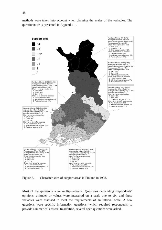
48

methods were taken into account when planning the scales of the variables. Thequestionnaire is presented in Appendix 1.

Figure 5.1 Characteristics of support areas in Finland in 1998.

Most of the questions were multiple-choice. Questions demanding respondents’opinions, attitudes or values were measured on a scale one to six, and thesevariables were assessed to meet the requirements of an interval scale. A fewquestions were specific information questions, which required respondents toprovide a numerical answer. In addition, several open questions were asked.

49

The method of data collection for the 1993 survey was mailing. The questionnairewith an accompanying note and a return envelope were sent to the 1207 farms on 1March 1993. Within three weeks 267 farms (22.1%) had returned the form. Afterthis, a reminder was sent and during four weeks 180 farms (14.9%) responded butbecause the rate was regarded as a too low, an additional reminder was sent, and afurther 100 farms (8.3%) returned the form. Thus the first set of data consisted of547 farms participating in the survey on risk and decision-making, and the responserate in 1993 was 45.3%.

The effect of nonresponse to the survey depends on the percentage not respondingand the extent to which these are biased (Fowler 1990, 48). The effect of nonre-sponse in 1993 was examined using two different methods. First, the data werecompared to the population using those variables which were available such asarable area, age of farmer, juridical form of farm, production line and location offarm. Minor differences were noted but they were not significant (Sonkkila 1996,78).

Secondly, the effect was studied in relation to the time the respondents returned theforms. This analysis is based on the idea that respondents interested in the topicreturn the form noticeably quicker than those who are less interested (Fowler 1990,49). If significant differences are found in relation to certain variables, it is likelythat nonrespondents differ from the data under these variables. As far as the 1993data set was concerned, the data were divided into three groups on the basis of thetime the forms were returned (those who responded immediately, those whoresponded after the first follow-up, and those who responded after the second

follow-up). Statistical tests (F-test and χ2 –test) were employed to test the groupsagainst all variables in the operational model.

The tests revealed that the groups did not differ significantly under any othervariable except education, which was higher for those who responded earlier(Sonkkila 1996, 79). For instance, Fowler (1990, 49) noted the relationshipbetween level of education to nonresponse. Therefore, it can be said that the datacorresponds to the population apart from the level of education, which is somewhathigher in the data than in the population.

In this study, the 1993 data are mainly utilised to compare the changes of farmers’objectives, values, attitudes toward risk, managerial issues and the significance ofuncertainty factors. In addition, it was also used when examining farms quittingproduction.

The second set consists of data from the rural business register on those 547 farmsin the 1993 survey. The variables taken from the rural business register arepresented in Appendix 2.

50

The questionnaire of the 1998 survey was designed on the basis of the 1993 surveyto follow-up possible changes that had taken place during the five years. However,some questions regarding adjustment into the EU were added and several questionswere omitted, because some data could be taken directly from the rural businessregister and some was not relevant in this study.

The 1998 survey was directed to only 468 farms of the 547 farms, because it wasknown in advance from the rural business register that 79 farms had ceased farmingduring 1993-1997. Of those 79 farms, 47 had quit before 1995 and the remaining32 farms had stopped between 1995 and 1997. The share of those quitting (2.9%yearly) was somewhat lower than in the population (3.7% yearly). The 1998 surveydid not address non-active farms, because the focus was on active farms, andbecause sufficient data on non-active farms were available in the 1993 survey andthe rural business register.

The method of data collection in the 1998 survey was mailing supplemented bytelephone contact. A questionnaire (Appendix 3) with an accompanying note(Appendix 4) and a return envelope were sent to the 468 farmers on 16 February1998. Within three weeks 269 farmers (57.5%) had returned the form; after this areminder, a new form and a return envelope were sent to the nonrespondents.During four weeks an additional 94 farmers (20.0%) responded. Finally, theremaining were called and persuaded to return the form as a result of which 52farms (11.1%) returned the form, so altogether 415 farms (88.7%) of the 468 farmstook part in the survey making up the third set of data on farmers’ decision-makingon adjustment in to the EU. The data of this study are the combination of thesethree sets of data.

Any bias in the 1998 study can be considered insignificant because of the highresponse rate (88.7%). However, possible bias due to nonresponse was studied bycomparing the three groups of respondents (those who responded immediately,those who responded after follow-up, and those who responded after telephonecontact) against the variables of the operational model. Statistical tests (F-test and

χ2 –test) indicated that the groups do not differ significantly against any variable inthe operational model so the reliability of the data due to nonresponse in 1998 canbe consider to be good.

In the data, the average size of farm is 32.1 ha, the share of rented land of total landis 19.6% and the average amount of basic support is FIM 84 000. The average ageof the farmer is 46.5. The main production lines are: dairy (39.2%), grain (28.5%),pig (7.9%), cattle (6.8%), other crop production (7.2%), and other (10.3%). Thejuridical form of the farm is divided into family-farms (92.1%), agriculturalconcerns (5.0%), and estates (2.8%). The share of on-farm incomes of all incomesis: full-time farmers 72.7%, additional income farmers 9.4%, and part-time farmers

51

17.9%. The distribution of the farms to support areas is: A (14.0%), B (28.4%), C1(21.5%), C2 (27.6%), C2P (3.5%), and C3C4 (5.0%).

In comparison to the population the average size of farm in the data set is 30%higher, the share of family-farms is higher, the share of estates is lower, the share offull-time farms is higher and the share of part-time farms is lower. Furthermore, theshare of dairy farms is higher and the share of farmers quitting farming is somewhatsmaller. This is consistent with the difference of farm size between the data andpopulation, because smaller farms are more likely to cease than bigger farms.However, the average age of farmer and the distribution of farms in differentsupport areas is similar in both the data and the population. The difference betweenthe data and the population is mainly due to the decision to limit the size of farmsto a minimum of 10 hectares in the 1993 survey.

To summarise, the farms in the data are somewhat larger with more full-time farmsthan in the population due to the 1993 decision to limit the size of farms to aminimum of 10 hectares. In addition, the data are biased in relation to the level ofeducation due to the rather low response rate in the 1993 survey; the educationallevel is somewhat higher in the data than in the population. Therefore the findingsand the results of the study cannot be generalised in terms of all active farms butrather towards somewhat bigger active farms with farmers with a better educationthan the average.

5.2 Methods of the study

The statistical analysis of the data was carried out using SYSTAT 5.03 forWindows –software. Variables of objectives, values, uncertainty factors and riskmanagement strategies were transformed by subtracting the given value from thenumber seven, when the greater value meant greater importance. Principalcomponent analysis was applied to objective and value variables in order tocombine information. Then, the resulting principal components were analysedagainst original variables and named. The data were described by distributions aswell as average and dispersion figures using tables and diagrams. Finally, theoperational model was tested by statistical tests.

The general objective of multivariate analysis is to compress the data in relation tovariables with some kind of dependency. Multivariate analysis requires thatvariables have at least moderate dispersion and correlate against other variables.Principal component analysis aims at describing the variation of original variablesby a smaller number of new variables, principal components (Chatfield and Collins1980, 55). These components are uncorrelated, linear combinations of originalvariables received by executing an orthogonal transformation of original variables.

52

The usage of principal components in subsequent analyses reduces computationaldifficulties (Mardia et. al. 1979, 244). Principal components may be calculatedfrom a correlation or covariance matrix, although the correlation matrix iscommonly used to avoid the scaling problem (Ranta et. al. 1989, 464). In this study,all principal components were calculated from a correlation matrix, because thestandard deviation was much greater for those variables with a small mean thanthose with a high mean, and this would therefore have had an harmful influence onthe analysis.

No objective criteria exist to assess the applicable number of principal components,even though the rules of thumb determine that the last included principal compo-nent should explain the variation no less than the original variables (Chatfield andCollins 1980, 72). In the case of a correlation matrix, components with at leasteigenvalue one are included. In practice, additional principal components may beaccepted as well if meaningful interpretation can be found for them. The interpreta-tion of principal components is based on the loading-matrix between componentsand original variables (Ranta et. al. 1989, 467). A deep interpretation can beobtained only if the original variables are multinormal (Ranta et. al. 1989, 464).However, the central limit theory proves that linear functions comply with normaldistribution even when the original data are not multinormal (Mardia et. al. 1979,60). Hence, adequate multinormality was assumed and therefore not tested in thisstudy.

The rotation procedure is commonly carried out to ease the interpretation of thecomponents. The VARIMAX-method, which is the most commonly used methodof rotation, aims at obtaining a few large loadings and many small loadings byabsolute value (Chatfield and Collins 1980, 73; Korhonen and Manninen 1993, 63).The VARIMAX-method was used in each principal component analysis in thisstudy. The interpretation and nomination of principal components is rathersubjective; the common method is to investigate the correlation between compo-nents and original variables, pick up large loadings by absolute value, and thenassess the common characteristics of the variables.

The basic difference between principal component analysis and factor analysis isthat while principal component analysis aims at finding linear combinations ofvariables explaining as much as possible the variation, factor analysis tries to findlatent variables behind the original variables (Korhonen and Manninen 1993, 61).Furthermore, factor analysis is based on a well-defined statistical model, whileprincipal component analysis is merely a transformation of the data (Mardia et. al.1979, 275). As implied by this, component scores in principal component analysiscan be accurately specified and used in subsequent analysis, whereas factor scoresin factor analysis have to be estimated (Chatfield and Collins 1980, 89). Becausethis study aimed at compressing variables into fewer sets of new variables, and

53

using the scores in further analysis, principal component analysis was chosen as themethod instead of factor analysis.

The dependent variable in this study, decision-making on adjustment into the EU,was nominal scale. Part of the independent variables were nominal, while the restwere interval or scale level variables. In this study, an analysis of two nominal scalevariables was based on cross-tables, and the statistical independence was tested by

Pearsons non-parametric χ2-test

h k

χ2 = ∑ ∑ (fij – eij)2 / eij

i=1 j=1

where h is a number of rows, k is a number of columns, eij is an expected fre-quency, and fij is an observed frequency. The null hypothesis of cross-table analysisstates that row and column variables are independent (Korhonen and Manninen1993, 17). The results of the cross-table analysis were mainly presented indiagrams.

In the case of nominal and interval or scale level variables, analysis of variance wasused, and the statistical independence was tested by the F-test

SSB/(k-1)F(k-1, N-k) = --------------- SSw/(N-k)

where F is the test of the null hypothesis that all groups have the same mean, N isthe total sample size, k is the number of groups, SSB is the sum of squares betweengroups, and SSw is the sum of squares within groups (Bray and Maxwell 1985, 18-19). The results of the analysis were mainly presented as tables.

When two interval or scale level variables were analysed, the statistical independ-ence was tested by the t-test

x1 - x2

t = ------------------------ (s1

2/n1 + s22/n2)

1/2

where x1 and x2 are the means, s12 and s2

2 are the variances, while n1 and n2 are thenumber of observations of the two variables (Bray and Maxwell 1985, 13-15). Thenull hypothesis of the t-test states that the variables have the same mean (Ranta et.al. 1989, 185). To test the hypothesis, a two-tailed test is used (see Ranta et. al.1989, 110). The results of the analysis were mainly presented as tables. In allanalyses, the result of the tests (statistical independence) were indicated as a

54

statistical significance (p)6. In the statistical tests, the population is expected to beinfinite, and the data set is used to approximate the population.

Analysis of variance was used in the study instead of analysis of regression,because the dependent variable (adjustment into the EU) is a qualitative, nominallevel variable. Analysis of variance does not presume a specific nature of thestatistical relationship between variables, while the basic analysis of regressionpresumes linear relationship for the parameters. In this study, the relationshipbetween dependent variable and independent variable is not necessarily linear, sothe presumption of linear relationship was too restrictive to test the operationalmodel. In addition, the regression coefficient was not relevant in this study.Furthermore, discriminant analysis allowed the investigation of the effect of severalindependent variables and their joint effect on the target variable in order tovalidate the results of the analysis.

The null hypothesis of one-way analysis of variance states that all groups have thesame mean, and the alternative hypothesis is that at least one of the groups has adifferent mean than other groups (Bray and Maxwell 1985, 14). Tukey’s pairwisetest can be used to determine which of the groups differ significantly from the mean(Neter et. al. 1990, 589). Analysis of variance presumes variables to be normallydistributed and to have homogenous variance (Bray and Maxwell 1985, 32-33).However, analysis of variance is rather stable to the deviations from the presump-tions, and the stability increases when the sample size increases (Ranta et. al. 1989,318). Therefore, analysis of variance was used instead of non-parametric methods.

Discriminant analysis aims at analysing the group differences in order to detect adiscriminant rule, which allows the clearest possible identification of the population(Korhonen and Manninen 1993, 68). A discriminant rule divides the space Rp intoseveral regions Ri (i=1,…,g); an observation belongs to the population Pk if itbelongs to the region Rk (Mardia et. al. 1979, 300). The linear combinations of thep variables are formed to best separate the k groups by maximising the between-group variance of the linear combination relative to the within-group variance(Bray and Maxwell 1985, 42-43). The maximum number of discriminant functionscannot exceed the number of variables and the number of groups subtracted by one.Wilk’s lambda7 provides a test to quantify the discriminant power of the model.Discriminant analysis was used to investigate the common effect of variables to theadjustment decision and to find out possible dependency between the variables.

6 Statistical significance p is reported as a decimal number (0.000≤ p ≤1.000) and it indicates theprobability that the null hypothesis is true. The smaller the p, the more obvious it is that the nullhypothesis can be rejected. The limiting value generally used in statistical tests is that the nullhypothesis can be rejected when p≤0.050.7 Wilk’s lambda L = |W|/|T|, where |W| is a determinant of the within-group matrix, and |T| is adeterminant of the sum of squares and products. The smaller the value of L, the better the groups canbe discriminated.

55

5.3 Transformation and condensation of the data

The dependent variable in the operational model, farmers’ decision-making onadjustment into the EU, is mainly based on the questions put to the farmers (seequestion B.1, variable b11 in Appendix 3). This variable was validated andspecified by the question of the second most important means of adjustment(question B.1, variable b12 in Appendix 3), as well as by an open questionconcerning the reasons behind the adjustment decision (question B.2 in Appendix3). Approximately 50% of the respondents answered the open question. Moreover,farmers’ chosen and given adjustment decisions were cross-checked against therural business register data. In other words, the decisions given by farmers werecompared to the changes that had taken place in the production and economicfactors of the farm. In the case of clear contradiction, the case was closely investi-gated in relation to various variables, and in some cases the dependent variable wasmodified. Altogether 26 cases were modified8. Because the dependent variable,farmers’ decision-making on adjustment into the EU, has been checked in quite anexhaustive way, the validity of the variable can be regarded to be adequate.

A principal component analysis was carried out in order to condense the informa-tion associated with the 18 objective-variables (see question C, variables c1-c18 inAppendix 3). The analysis was carried out on 362 observations; nonrespodents andmissing data were excluded, and farmers who had quit were not asked the ques-tions. Five principal components were chosen for the forthcoming analysis, becausethe eigenvalue of the fifth component was 1.070, while the eigenvalue of the sixthcomponent was 0.948, and the sixth principal component did not provide additionalinformation. Appendix 5 illustrates the matrix of rotated loadings. Together the fiveprincipal components explain 57.6% of the variation of original objective variables.

The first principal component loads best to increasing size of farm, expandingproduction, acquiring new and bigger machinery and buildings, and ensuringcontinuation. The principal component is clearly associated with development andexpansion of farms and production. The second principal component is associatedwith risk reduction, small loans in relation to assets, avoiding losses, and main-taining liquidity. The principal component is closely connected to risk reduction.

The third principal component loads to increasing profit, raising total incomes,improving return of capital, increasing amount of supports and expanding property.The component is associated with increase of returns. The fourth principalcomponent is associated with increasing household spending and leisure time, andimproving the quality of life. The component is linked to the improvement of

56

household life. The fifth principal component is related to taking care of theenvironment, improving the quality of products and maintaining liquidity. Thecomponent is associated with the production of quality products in an environmen-tally sustainable way.

On the basis of the preceding analysis, the principal components were named in thefollowing way (code and number in parenthesis represent code of a new principalcomponent variable and how much each principal component explain the variationof the original variables).

1. Develop farm and production (C2PCA1, 15%)

2. Decrease risk (C2PCA2, 10%)

3. Increase returns (C2PCA3, 15%)

4. Increase household spending and leisure (C2PCA4, 9%)

5. Produce environmentally sustainable quality products (C2PCA5, 9%)

A second principal component analysis was carried out in order to condense theinformation associated with the 17 value variables (see question F, variables f1-f17in Appendix 3). The analysis was performed on 365 observations excludingnonrespodents, and farmers who had quit were not asked the questions. Fourprincipal components were chosen for the forthcoming analysis, because theeigenvalue of the third component was 1.017, while the eigenvalue of the fourthcomponent was 0.926, and the fourth principal component did provide additionalinformation. Appendix 6 illustrates the matrix of rotated loadings. Together thefour principal components explain 58.3% of the variation of original variables.

The first principal component loads best to the possibility of having reasonableincomes, making profit, job assurance and to respect gained from work. Theprincipal component is associated with instrumental values derived from farmwork. The second principal component is associated with the way of life, outdoorlife and environmentally friendly production. The principal component is closelylinked to the intrinsic value of farming life itself.

The third principal component loads best to belonging to a farm community, to thepossibility of expanding production, self development and to respect gained fromwork. The component is associated with the social and expressive value ofmeaningful work. The fourth principal component is associated with workindependence, versatility, doing work one chooses, self development, the potentialto express oneself, entrepreneurship, and challenging work. The component islinked to expressive and intrinsic values of entrepreneurship in the countryside.

8 The most important means of adjustment and the second most important means of adjustment wereswitched, when the open question and other variables clearly indicated that the answer should be theother way around.

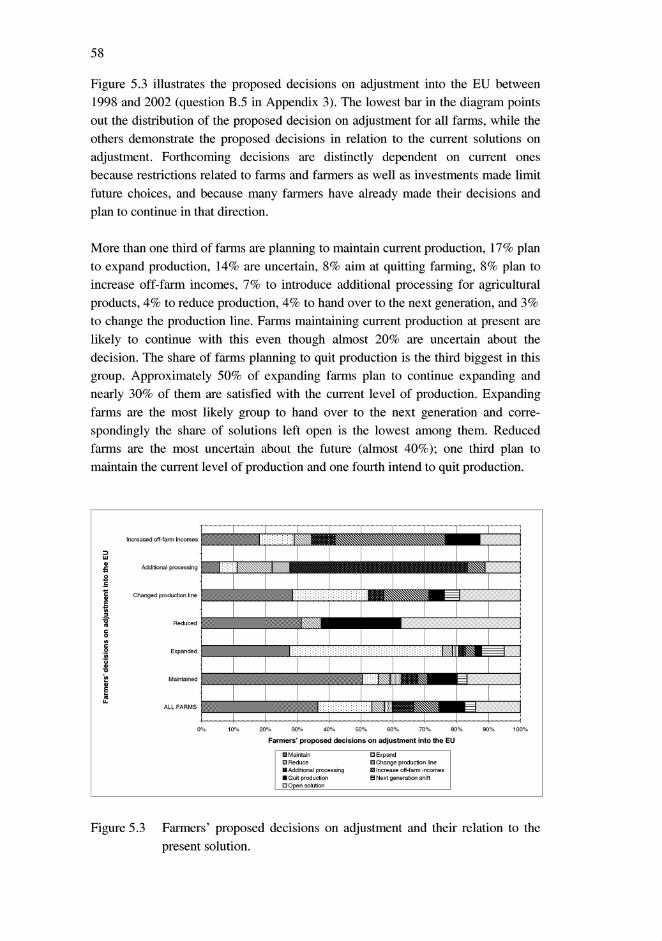
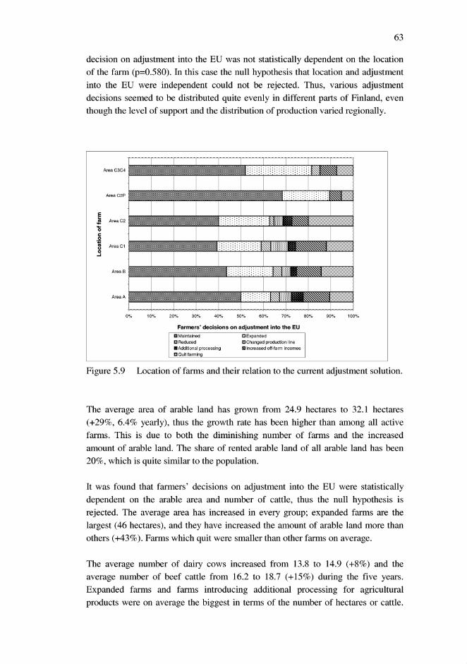
66

Full-time farms consisted of more expanded and maintained farms, while the shareof farms which increased off-farm incomes and farms which reduced productionwas greater then on average among part-time farms. The major reason for this isthat expanded and maintained farms consist of more cattle farms demanding morelabour.

5.4.4 Farmer-related factors

5.4.4.1 Age, life cycle, successor and education

The average age of farmers has grown by 0.6 years during the period 1993-1998and, at the same time, the time lapse for the change from the previous generation(question A.2 in Appendix 3 and question A.20 in Appendix 1) has grown by 1.1years (Table 5.4). Farmers’ decisions on adjustment into the EU were statisticallydependent on the age and time lapse for the change from the previous generation,thus the null hypothesis was rejected. Farmers introducing additional processing foragricultural products, farmers who increased off-farm incomes and farmersexpanding were younger than average, while farmers decreasing production andthose maintaining current production were distinctly older. The same holds true forthose handing over to the next generation. For farms changing their main produc-tion line there have been percentually more shifts from one generation to the next,because the time lapse has gone down. Changes in the main line of productionfrequently occur during the change to the next generation or just after.

Table 5.4 Farmers’ age and time lapse from the previous generation to the nextand their relation to the current adjustment solution.

Age and lifecycle offarmer

n Mean Main-tained

Ex-panded

Reduced Chan-ged

produc-tion line

Addi-tionalproc-

essing

In-creased

off-farmincome

Quit Risk(p)

Farmers’ agein 1998Farmers’ agein 1993

466

547

46.5(10.5)

45.9(12.0)

48.5(10.5)

46.2(11.2)

43.5(9.3)41.4(9.8)

54.6(11.4)

50.8(9.7)

47.5(12.2)

46.8(13.1)

41.3(9.7)39.2

(10.5)

42.9(9.1)41.6

(10.7)

--

54.4(13.2)

0.000

0.000

Years fromlast gener.shift in 98Years fromlast gener.shift in 93

389

509

18.5(10.4)

17.4(11.8)

20.4(10.3)

17.5(11.5)

15.9(8.7)

14.6(10.7

25.7(12.2)

20.9(11.5)

16.0(11.4)

17.3(10.2)

17.1(10.4)

14.2(10.5)

15.5(10.7)

15.0(12.6)

--

31.5(9.2)

0.000

0.000

Standard deviation is presented in parenthesis.

The timing of the shift to the next generation on the farm is illustrated in Figure5.11 (question A.5 in Appendix 3 and question A.21 in Appendix 1). 15% of farmsplan to do this in five years, 32% of farms plan that the shift will take place

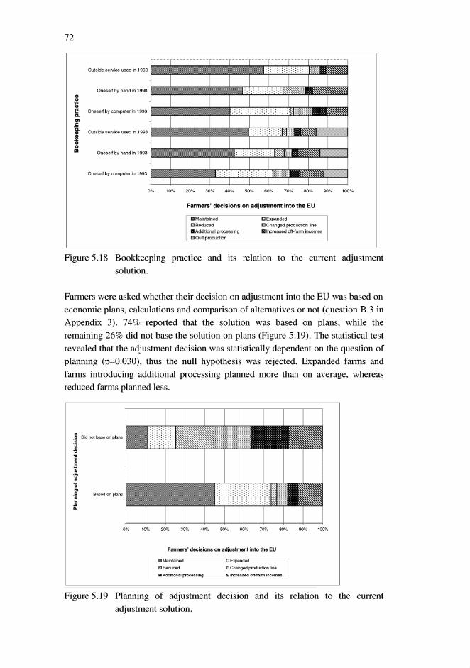
73

Farmers were asked a simplified question related to their attitudes toward risk10.According to this risk measure, 79% of farmers were risk averse, 16% were riskneutral and 5% were risk takers (Table 5.5). On average, farmers were ready to payFIM 24.3. Farmers’ decisions on adjustment into the EU were statistically depend-ent on their attitudes toward risk, thus the null hypothesis was rejected. Farmersincreasing off-farm incomes and changing their main production line were onaverage the least risk averse farmers. The level of aversion to risk had lowered inall other groups except expanded farms.

Table 5.5 Farmers’ attitudes toward risk and its relation to the current adjust-ment solution.

Farmers’attitudes

toward risk

n Mean Main-tained

Ex-panded

Reduced Chan-ged

produc-tion line

Addi-tionalproc-

essing

In-creased

off-farmincome

Quit Risk(p)

Attitudetoward riskin 1998Attitudetoward riskin 1993

356

429

24.3(21.0)

22.1(17.3)

22.3(20.0)

19.1(16.2)

20.7(18.3)

23.2(16.5)

19.4(19.6)

13.6(13.1)

32.3(23.2)

30.5(17.2)

24.9(20.3)

19.7(14.4)

35.1(25.2)

26.4(17.7)

--

26.3(21.1)

0.001

0.002

Standard deviation is presented in parenthesis.

5.4.4.3 Objectives and values

Farmers were asked to estimate the importance of 18 different objectives (seequestions c1-c18 in Appendix 3) on the farm and to the farm-family using a scale ofone (very important) to six (not important). Most of the questions were similar tothe questions presented in 1993 to the same group of farmers. The most importantobjectives were ensuring liquidity, avoiding losses, taking care of the environment,improving the quality of life, and reducing risk (Figure 5.20). The priorisation ofobjectives during the five years remained quite stable, although the environmentalobjective has been emphasised and the quality objective lowered.

10 The question concerned a game situation, where respondents were asked how much they would bewilling to pay for a lottery ticket, where a chance to gain FIM 100 was 50% and to gain FIM 0 wasalso 50% (P(0)=0.5 and P(100)=0.5) (see question G.2 in Appendix 3 and question I.4 in Appendix1).

74

Figure 5.20 Farmers’ assessment of the importance of objectives.

The priorisation of the objectives in relation to the adjustment decision werecompared using five objective principal components (develop farm and production,decrease risk, increase returns, increase household spending and leisure, andproduce environmentally sustainable quality products) (Table 5.6).

Table 5.6 Objectives and their relation to the current solution.Farmers’ objectives Main-

tainedEx-

pandedReduced Chan-

gedproduc-tion line

Addi-tionalproc-

essing

In-creased

off-farminocme

Risk(p)

Develop farm and production

Decrease risk

Increase returns

Increase household spendingand leisureProduce environmentallysustainable quality products

-0.14(0.97)-0.03

(0.96)-0.01

(1.04)0.01

(0.99)0.00

(0.94)

0.49(0.93)

0.10(0.85)

0.07(0.89)-0.09

(1.02)0.09

(0.94)

-1.07(0.60)-0.36

(1.70)-0.67

(1.32)0.14

(0.76)0.08

(1.33)

-0.11(0.93)

0.13(0.91)

0.08(0.96)-0.05

(0.94)-0.02

(1.24)

0.08(0.99)

0.53(0.61)

0.07(1.23)

0.12(0.91)-0.02

(1.52)

-0.21(0.98)-0.24

(1.24)-0.02

(0.94)0.11

(1.12)-0.15

(0.94)

0.000

0.065

0.346

0.863

0.838

Number of cases for each objective 363, mean 0.000 and s=1.000; higher value means greater importance.Standard deviation is presented in parenthesis.

The objective to develop the farm and production was the only statisticallydependent variable on the adjustment decision, though the objective to decreaserisk was almost dependent. Developing the farm and production was the mostimportant for farmers expanding, and the least important for those reducing

1 2 3 4 5 6

Ensuring liquidity

Avoiding losses

Taking care of the environment

Improving quality of life

Reducing risk

Increasing supports

Improving profit from capital

Increasing total incomes

Maintaining a low degree of debt to assets

Improving quality of products

Increasing profit

Increasing leisure

Ensuring continuity

Increasing assets

Increasing farm size

Expanding production

Obtaining new and bigger machinery and buildings

Increasing household spending

75

farming. Decreasing risk was the most important for farmers introducing additionalprocessing for agricultural products and the least important for those reducingfarming and increasing off-farm incomes.

Farmers were asked to estimate the importance of 17 different values in farmmanagement (see questions f1-f17 in Appendix 3) using a scale of one (veryimportant) to six (not important). Most of the questions were similar to thequestions presented in 1993 to the same group of farmers. The most importantvalues were independence of work, versatility of work, the possibility to do workone likes, lifestyle, and the possibility to earn reasonable incomes (Figure 5.21).During the five years, the importance of various values stayed almost identical; thevalue of environmental issues in production rose slightly, while the value ofentrepreneurship dropped.

Figure 5.21 Farmers’ assessment of the importance of values.

The importance of the values in relation to the adjustment decision were comparedusing four value principal components (earning, farming lifestyle, meaningful workand entrepreneurship in the countryside) (Table 5.7). Each of these components wasstatistically dependent on the adjustment decision. Earning was the most importantto reducing and expanding farmers and the least important to those increasing off-farm incomes and those adding processing for agricultural products. Farminglifestyle was the most important value for farmers reducing and maintaining currentproduction and the least important for farmers expanding, introducing additionalprocessing for agricultural products and changing their production line.

1 2 3 4 5 6

Independence of work

Versatility of work

Possibility to do work one likes

Lifestyle

Possibility to receive reasonable incomes

Job assurance

Entrepreneurship

Challenge in work

Possibility to express oneself

Environmentally friendly production

Continuing family farm

Outdoor life

Possibility to develop oneself

Possibility to gain profit

Respect received from work

Belonging to a farm community

Possibility to expand production

76

Table 5.7 Values and their relation to the current solution.Farmers’ values Main-

tainedEx-

pandedReduced Chan-

gedproduc-tion line

Addi-tionalproc-

essing

In-creased

off-farminocme

Risk(p)

Earning

Farming lifestyle

Meaningful work

Entrepreneurship in thecountryside

0.07(0.91)

0.16(0.89)-0.01

(0.95)0.01

(0.92)

0.23(0.87)-0.32

(1.04)0.20

(0.94)0.11

(0.92)

0.29(1.25)

0.47(1.47)-0.96

(1.52)-0.75

(1.61)

-0.11(0.89)-0.22

(1.00)0.34

(1.00)0.14

(0.58)

-0.25(1.45)-0.22

(0.94)0.15

(0.85)0.33

(0.93)

-0.51(1.12)

0.06(1.05)-0.24

(1.04)-0.27

(1.28)

0.000

0.003

0.001

0.039

Number of cases for each objective 366, mean 0.000 and s=1.000; higher value means greater importance.Standard deviation is presented in parenthesis.

Meaningful work was the most important to farmers who changed their productionline, expanded farming and for farmers who added processing for agriculturalproducts, while those reducing farming and increasing off-farm incomes regardedmeaningful work as the least important. Entrepreneurship in the countryside wasthe most important for farmers introducing additional processing for agriculturalproducts and the least important for those reducing farming and increasing off-farmincomes.

5.4.5 Operational environment

Farmers were asked to estimate the significance of nine different factors causinguncertainty on the farm (see questions d1-d9 in Appendix 3) using a scale of one(very significant) to six (not significant). The questions were similar to thosepresented in 1993 to the same group of farmers, although the amount of variableswas much smaller. The most significant uncertainty factors were changes inagricultural policy, maintaining liquidity, variations in product prices, accidents,and outlets for products. The relative significance of various factors of uncertaintyhad somewhat altered; changes in agricultural policy were more highlighted, whilesales of products and availability and adequacy of funding were regarded as lesssignificant in 1998 than in 1993.

The significance of the uncertainty factors was compared in different groups (Table5.8). Out of the nine uncertainty factors, five were statistically dependent on theadjustment decision.

77

Table 5.8 Uncertainty factors and their relation to the current solution.Significance of

uncertainty factorsMean Main-

tainedEx-

pandedRe-

ducedChan-

gedproduc-tion line

Addi-tionalproc-

essing

In-creased

off-farm

income

Risk(p)

Changes in agriculturalpolicyMaintaining liquidity

Variations in product prices

Accidents

Outlets for products

Adequacy of ones ownknowledge, skills andeducationProduction risk

Development andintroduction of newtechnologyAvailability and adequacyof funding

5.38(1.00)

5.33(0.99)

5.10(1.17)

4.71(1.25)

4.67(1.44)

4.50(1.36)

4.43(1.34)

3.78(1.43)

3.76(1.77)

5.36(1.01)

5.39(0.91)

5.16(1.13)

4.72(1.25)

4.76(1.40)

4.55(1.26)

4.49(1.31)

3.66(1.38)

3.86(1.79)

5.59(0.69)

5.49(0.81)

5.18(1.08)

4.60(1.22)

4.63(1.33)

4.66(1.35)

4.43(1.29)

4.21(1.31)

4.01(1.66)

5.82(0.60)

5.00(1.55)

5.00(1.41)

5.09(1.30)

4.73(1.62)

3.64(1.80)

5.00(1.41)

2.64(1.96)

2.55(2.02)

5.29(0.90)

5.19(0.93)

5.24(1.09)

4.62(1.24)

4.86(1.42)

4.62(1.07)

4.29(1.42)

3.67(1.59)

3.24(1.70)

5.63(0.81)

5.50(0.89)

5.44(0.81)

5.31(0.87)

5.06(1.18)

5.13(1.41)

4.81(1.05)

4.19(1.52)

3.88(1.93)

4.91(1.39)

4.94(1.32)

4.66(1.45)

4.64(1.36)

4.23(1.71)

4.04(1.53)

4.02(1.53)

3.53(1.41)

3.43(1.72)

0.001

0.020

0.074

0.335

0.197

0.008

0.116

0.001

0.043

Number of cases 367, scale from 1 to 6 (1=not significant, 6=very significant).Standard deviation is presented in parenthesis.

Availability and adequacy of funding were the least important factors to reducedfarms and to farms which changed their production line. Adequacy of ones ownknowledge, skills and education were the most important for farms introducingadditional processing for agricultural products and the least important for reducedfarms and those increasing off-farm incomes. Changes in agricultural policy wereregarded as the most important by farms reducing production, while farmsincreasing off-farm incomes considered it the least important. Maintaining liquiditywas the least important for reduced farms and for farms which increased off-farmincomes. Development and the introduction of new technology were the mostimportant for expanded farms and for farms adding processing for agriculturalproducts and the least important for reduced farms.

Farmers were asked to estimate the importance of five risk management strategieson the farm (see questions e1-e5 in Appendix 3) using a scale of one (veryimportant) to six (not important). The questions were similar to the questionspresented in 1993 to the same group of farmers, although the amount of variableswas much smaller. The most important risk management strategies were maintain-ing adequate liquidity and solvency, and planning and controlling production andeconomy. The relative importance of risk management strategies remained ratherstable during the five years.

78

The importance of risk management strategies was compared in the differentgroups (Table 5.9). Each of these five variables was statistically dependent on theadjustment decision. Planning and controlling production and economy was theleast important for reduced farms. Obtaining off-farm incomes was the mostimportant for farms involved in that and for farms introducing additional process-ing for agricultural products, and the least important for expanded farms. Contractproduction was the least important for reduced farms, and maintaining adequateliquidity and solvency the least important for farms which increased off-farmincomes. Diversification was the most important for farms which made additionalprocessing for agricultural products and the least important for reduced farms.

Table 5.9 Farmers’ assessment of the importance of risk management strategies.Importance ofrisk manage-

ment strategies

Mean Main-tained

Ex-panded

Re-duced

Chan-ged

produc-tion line

Addi-tionalproc-

essing

In-creased

off-farm

income

Quit Risk(p)

Maintainingadequate liquidityand solvencyPlanning andcontrollingproduction andeconomyObtaining off-farm incomesContractproductionDiversification

5.47(0.86)

5.14(1.15)

4.26(1.68)

4.11(1.60)

3.51(1.52)

5.49(0.79)

5.21(1.05)

4.14(1.60)

4.18(1.55)

3.60(1.43)

5.63(0.59)

5.37(0.90)

3.47(1.65)

4.28(1.57)

3.29(1.53)

5.64(0.67)

3.64(1.96)

4.27(2.28)

2.64(1.86)

2.73(2.28)

5.48(0.68)

5.10(1.34)

4.39(1.60)

3.86(1.68)

3.91(1.55)

5.47(1.30)

5.33(0.98)

5.20(1.42)

4.07(1.75)

4.40(1.18)

5.07(1.26)

4.76(1.35)

5.74(0.62)

3.98(1.60)

3.33(1.57

--

--

------

0.010

0.000

0.000

0.040

0.024

Number of cases 368, scale from 1 to 6 (1=no important, 6=very important).Standard deviation is presented in parenthesis.

Utilisation of risk management strategies is a part of farm management and thus apart of the farmers’ decision-making on adjustment into the EU. The variables werestatistically dependent, and the nature of dependency was consistent, hencefarmers’ evaluation of the importance of risk management strategies can beconsidered to confirm the validity of independent variables on decision-making onadjustment into the EU.

5.5 Characteristics of farms and farmers according to the

decision on adjustment into the EU

The farms which maintained current production are close to the average for farmsand farmers as far as the size of farm, incomes and debts, share of on-farm incomesof all incomes and characteristic of farmer are concerned. Farmers maintaining

79

production are on average two years older than farmers in general and the share ofanimal farms among them is bigger than the average. The farmers themselves donot distinctly prioritise various objectives or values. However, the intrinsic value offarming lifestyle seems to be the most important to them. The most commonanswers to their intention to adapt in the future are to continue to maintain currentproduction with added reservations about future decisions.

On closer examination, it was found that this group could be differentiated bycertain factors on the basis of the question of intention to invest during the next fiveyears. 36% intended to refrain from making investments during the period 1998-2002. For these farms, the prioritisation of the objective of developing the farm andproduction was much lower than the rest of the maintained farms. In addition, theobjective of producing environmentally sustainable quality products was lower thanfor those farms intending to refrain from making investments. These farms weresomewhat smaller as far as the size, number of animals and income were con-cerned, and the age of the farmer was two years older than the rest of farmersmaintaining production. However, the production line, support zone, share of on-farm incomes of all incomes, values and attitudes toward risk did not differbetween these two groups. Farms intending to refrain from investing were alsomuch more unsure about the future direction; 50% of the farms intended to quitproduction or indicated that the matter was open. The successor was known to only10% of the above mentioned farms, while 32% of the rest of farms maintainingproduction had a successor. It was found that in the group of farms maintainingcurrent production, the share of those quitting in 1998-2000 was considerablyhigher among those farms which stated that they would refrain from makinginvestments than for those maintaining current production.

In conclusion, the majority of farms maintaining current production decided tocontinue this line because they were ready to make at the very least investments tokeep their production in operation, and they were quite sure about the future. Evenso, about one third were either planning to quit production or were unsure aboutfuture decisions. In the meantime they keep producing without investing. Thematter of a successor is bound to be one of the decisive questions for these farmers.

In the open question (see question B.2 in Appendix 3) farmers put forward severalreasons for maintaining current production. Some stated that age or health did notpermit alternatives. Uncertainty about a successor was one of the reasons as well.Some emphasised the uncertain environment and a hard situation in farm economyleading to caution in decision-making as well as an unwillingness to makeinvestments and to take an additional debt. In other cases, the small size of farm,small milk quotas, or low levels of labour or financial resources were the majorreasons behind their decisions. In other words, farmers felt they did not have otheroptions. To summarise, production and economy of the farm, the situation of the

80

farmer and farm-family as well as the assessment of the operational environmentwere mentioned in the farmers’ answers. Therefore, the factors underpinningdecisions are diverse and vary from one farmer to another.

The farms which expanded production are mostly animal farms and on averagelarger when measured by arable area and number of animals. Consequently, theiron-farm incomes and level of debt are also higher than average, and they are mostlyfull-time farmers. They are better educated, younger, more risk averse, and utilisemore modern management practice than average farmers. They prioritise theobjective of developing the farm and production to other objectives. The instru-mental value of earning as well as the social and expressive values of meaningfulwork are important to them, while the intrinsic value of farming lifestyle issignificantly less important. The most common answers to their intentions to adaptin the future are to continue expanding and to maintain current production.

In the open question farmers explained the choices of expanding in the followingway: a high level of debt forces one to expand, ensuring continuity and viability ofthe farm for transfer to the next generation, the possibility to buy additional landfrom nearby farms, a farm family has extra labour to increase production, moreefficient use of machinery, securing income levels, the possibility to get investmentsupport, no other possibilities except agriculture in the countryside, and a farmeryoung enough to develop and expand. Like farms maintaining production, allfactors of the operational model were mentioned as reasons to expand production.

The farms which reduced production are on average smaller farms, whose mostcommon production line is grain. Thus their on-farm incomes and debts are lowerthan average, and about half of them are part-time or additional income farms.Farmers reducing production are less educated, older and more risk averse thanaverage farmers, and they do not utilise modern management practice so much.Increasing household spending and leisure are more prioritised objectives for themthan development and increasing returns. Of the values, farming lifestyle andearning are important, whereas meaningful work and entrepreneurship in thecountryside are less important. The most common answers to their intentions toadapt in the future are uncertainty, maintaining current production, and quitting.These farms are the most uncertain about the future and relatively the biggest groupto quit farming.

In the answers to the open question, the EU, age and health of the farmer, unprofit-able production and willingness to decrease work were mentioned as the reasonsbehind reducing production.

The farms which changed their production line are somewhat smaller in arable areaand number of animals, and they are mostly crop farms. Their on-farm incomes and

81

debts are also lower than average. Farmers changing current production lines areaverage in age and better educated, utilise modern management practice more andare less risk averse than farmers on average. Objectives are not clearly prioritised,whereas meaningful work is regarded as the most important value and farminglifestyle as the least important. The most common answers to their intentions toadapt in the future are maintaining current production, expanding, and uncertainty.

To the open question, farmers explained their solutions in terms of profitability, theEU, a successor, health (allergy or asthma), willingness to leave animal production,and taking an interest in organic production.

The farms which introduced additional processing for agricultural products arelarger than average farms but consist of more crop farms than farms expandingproduction. Thus their on-farm incomes and debts are higher than average, whilethe share of full-time farms is lower. These farmers are younger than other farmers,better educated than the average, and utilise modern management practice more.Risk reduction is the most important objective and entrepreneurship the mostimportant value. Earning and farming lifestyle are the least important values. Themost common answers to adaptation in the future are adding processing foragricultural products, uncertainty and reducing production.

To the open question the low income level of agricultural production, a higherdegree of interest in additional processing than in basic agricultural production, andthe possibility and resources to exercise additional processing were mentioned.

The farms which increased off-farm incomes are on average smaller farms, whosemain production line is grain. Their on-farm incomes are lower but their debts arehigher than average. The share of part-time farmers among the group is higher thanin any other group. Farmers increasing off-farm incomes are younger than average,have a better basic education, utilise modern management practice in an averageway, and they are less risk averse than other groups. Increasing household spendingand leisure are the most important objectives for them, whereas decreasing risk anddeveloping are the least preferred. These farmers regard diversification to off-farmwork as an adequate method of risk reduction, which can also be noted by the factthat they assess obtaining off-farm incomes as the most important risk managementstrategy. The most important value is farming lifestyle, while earning, meaningfulwork and entrepreneurship in the countryside are not so important. The mostcommon answers to their intentions to adapt in the future are further increasing off-farm incomes, maintaining current production, and uncertainty.

To the open question farmers explained their solutions in terms of low profitabilityand income levels, small farm size, adequacy of money, uncertainty in agricultureand the possibility to stabilise income by getting part of it outside agriculture. Some

82

farmers also emphasised the availability of off-farm income as well as furthereducation of the farmer or spouse enabling them to work outside the farm.

The farms quitting production are on average smaller farms, whose main produc-tion lines are mostly dairy or grain. Their on-farm incomes are lower than averagebut their debts are average. Those quitting are clearly older, less educated andutilise less modern management practise than farmers on average. Farms quittingprioritise objectives associated with expanding and ensuring continuity the least.The most important value is intrinsic value, whereas instrumental and expressivevalues were the least important.

The timing of this study enabled the examination of farmers who had quit produc-tion after the survey; during the period 1998-2000. Altogether 47 of 468 farms quitproduction during the three years, so the share has been 3.3% yearly. The share inthe year 2000 was higher than in 1998 or in 1999. This is probably due to Agenda2000, under which farmers were to commit themselves to a new period of six years.Farmers quitting between 1998-2000 were quite similar to those who had quitproduction during 1993-1997.

Upon examination in terms of their intentions to future adaptation it was revealedthat 38% intended to quit during the five years, 23% were unsure and 13% intendedto maintain current production. The intentions seemed to correspond quite well totheir real behaviour; farmers who stated their adjustment strategy were alsocommitted to continuing production by following this strategy. The intention to quitfarming was higher for those farms who had quit production in 1998 or in 1999(60%), while the level of unsureness was higher for farmers who had quit produc-tion in 2000 (28%). The time period, therefore, affects how well the intentioncorresponds to real behaviour. Moreover, some of the farmers intending to continuemaintaining current production had obviously not made a clear, conscious, strategicadjustment decision but rather decided to keep production as it was for a while andto observe changes in the operational environment.

The original adjustment decision on coming into the EU for farms quittingproduction differed from average farms: the share of reduced farms, farmsincreasing off-farm incomes and farms maintaining current production were higher,while the share of expanded farms was lower. Farmers quitting prioritised objec-tives related to development and risk reduction low, while farming as a lifestylewas a more important value for them than for farms continuing. The share of full-time farms (74%) as well as dairy farms (43%) and other crops farms (13%) amongthose quitting was higher than average. Therefore, small dairy and crop farms withaged farmers are the most likely to quit production. Table 5.10 summarises thecharacteristics of farms and farmers according to the decision on adjustment intothe EU.

83

Table 5.10 Characteristics of farms and farmers according to the decision onadjustment into the EU.

Adjustment decision CharacteristicsMaintained production • Quite average farms and farmers.

• More animal farms than average.• Somewhat older than average farmers.• Intrinsic values are important.• Quite uncertain about the future.

Expanded production • Mostly full-time animal farms.• Larger than average farms.• Better educated and younger than average farmers.• More risk averse than average farmers.• Utilising more modern management practice than average.• Instrumental, social and expressive values are important.• Development is an important objective.• Future is quite clear.

Reduced production • Smaller, mainly grain farms.• More part-time or additional income farms than average farms.• Less educated and older than average farmers.• More risk averse than average farmers.• Utilising little modern management practice.• Intrinsic and instrumental values are important.• Uncertain about future.

Changed their production line • Mostly crop farms, which somewhat smaller than average farms.• Better educated, average age farmers.• Utilising more modern management practice than average.• Less risk averse than average farmers.• Expressive values are important.• Future is quite clear.

Introduced additionalprocessing for agriculturalproducts

• Larger, mostly crop farms.• Better educated and younger than average farmers.• Utilising more modern management practice than average.• Instrumental values are important.• Future is quite clear.

Increased off-farm incomes • Smaller, mostly part-time grain farms.• Younger than average farmers.• Less risk averse than average farmers.• Intrinsic values are important.• Quite certain about the future.

Quit production • Smaller, mostly dairy and other crop farms• Less educated and older than average farmers.• Utilising less modern management practice than average.• Intrinsic values are important.

Discriminant analysis was used to test how the most significant variables in theoperational model were able to discriminate the farms into groups according to thedecision on adjustment into the EU. The basic criterion for choosing variables wasthe significance in one-way analysis of variance (F-test). In addition, the aim was touse continuous variables, and to have at least one production, economic and farmer-related variable in the analysis. Several trials were carried out using differentcombinations of variables in order to find an effective discriminant function usingas low a number of variables as possible.

It was found that the ability of discriminant functions to discriminate was ratherlow even though the number of variables was increased considerably. Wilk’s

84

lambda varied between 0.5 and 0.6, and correspondingly only 40-50% of theobservations could be grouped into the right classes. The correctness of classifyingvaried from 25% to 63% depending on the group. The biggest group, farmsmaintaining current production, could not be classified properly, while thoseexpanding and reducing could be more easily grouped into the right classes. Whenthe group of farms maintaining current production was omitted from the analysis,about 60% of the observations could be correctly classified, and Wilk’s lambda was0.4. In addition, almost 70% of the observations were able to be discriminated intofarms continuing and quitting.

Appendix 8 presents a discriminant analysis, where the discriminant variables areage of farmer, arable area, objective of developing the farm and production,agricultural incomes, attitudes toward risk, value of meaningful work and produc-tion line. In this analysis, Wilk’s lambda was 0.51, and three discriminant functionswere statistically significant. By examining the canonial loadings (correlationbetween dependent variables and canonial factors) it was revealed that the firstdiscriminant function correlated positively to arable area, to the objective ofdeveloping the farm and production and to agricultural incomes; the secondcorrelated negatively to age, positively to lower attitude toward risk and to cropfarms instead of animal farms; and the third correlated positively to age, to arablearea and to crop farms instead of animal farms.

Even though the analysis fails to predict accurately enough the adjustment decisionon the basis of the significant variables in the operational model, by examining themisclassifications, the tests revealed which of the groups were close together. Inparticular, farms expanding and introducing additional processing for agriculturalproducts seemed to be very similar on the basis of the analysis. Farms reducing andthose maintaining current production were somewhat closer each to other thanother groups as was the case for farms changing their production line and thoseincreasing off-farm incomes.

Another indication of the discriminant analysis was that even though the factors ofthe operational model individually explained decisions on adjustment into the EU,the joint effect of these variables and thus their joint ability to explain decisionswas not any clearer than any single factor alone11. Thus, the effect, relationship andmagnitude of the factors in the operational model to decision-making vary in thedata. In the light of this analysis, the operational model consisting of factorsaffecting farmers’ adjustment decisions, and the relative importance and relation-ship of these factors greatly depend on the farmer and the farm.

11 The correlation of the variables of the operational model was not high.

85

5.6 Changes in farmers’ objectives, values, attitudes toward risk,

managerial issues and the significance of uncertainty factors

The second objective of the study was to examine possible changes in farmers’objectives, values, attitudes toward risk, managerial issues, and the significance ofrisk factors in the EU environment (year 1998) compared to the environment beforeaccession (1993). The changes were also compared with the different groupsinvolved in decision-making on adjustment. The prioritisation of the mostimportant objectives had remained quite stable; ensuring liquidity and reducing riskwere the most significant objectives (Table 5.11).

Table 5.11 Comparison in changes in objectives.Objective Mean in

1998Mean in

1993Diffe-rence

Risk(p)

Increasing farm size

Ensuring continuity

Improving quality of life

Increasing profit

Improving return of capital

Avoiding losses

Increasing leisure

Expanding production

Improving quality of products

Increasing assets

Ensuring liquidity

Taking care of the environment

Increasing total incomes

Maintaining a low degree of debt to assets

Increasing household spending

Obtaining new and bigger machinery and buildings

Reducing risk

Increasing supports

3.14(1.71)

4.23(1.76)

4.88(1.28)

4.33(1.49)

4.66(1.26)

5.39(1.13)

4.26(1.53)

3.12(1.61)

4.38(1.56)

3.36(1.59)

5.43(0.98)

4.93(1.14)

4.56(1.34)

4.48(1.62)

2.39(1.28)

2.41(1.43)

4.84(1.19)

4.78(1.43)

3.53(1.84)

4.68(1.67)

4.71(1.43)

4.68(1.29)

4.78(1.30)

5.58(0.88)

3.71(1.61)

3.63(1.68)

5.41(1.04)

3.54(1.60)

5.61(0.81)

5.14(1.01)

4.14(1.46)

5.16(1.12)

2.34(1.36)

2.50(1.35)

n.a.

n.a.

-0.62(1.87)-0.57

(1.88)+0.19(1.64)-0.41

(1.67)-0.17

(1.58)-0.14

(1.31)+0.47(1.80)-0.60

(1.77)-1.10

(1.68)-0.23

(1.82)-0.18

(1.15)-0.17

(1.30)+0.34(1.67)-0.64

(1.83)+0.07(1.63)-0.15

(1.66)-

-

0.000

0.000

0.029

0.000

0.042

0.056

0.000

0.000

0.000

0.022

0.017

0.017

0.000

0.000

0.430

0.149

-

-

Number of cases 363 in 1998 and 480 in 1993, scale from 1 to 6 (1=not important, 6=very important). N.a.means that the question was not asked in the 1993 survey. Means in 1998 and in 1993 are calculated with allcases. However, the difference between objectives in 1993 and in 1993 is calculated in pairs, thus thedistinction between mean in 1998 and mean in 1993 differs from the column ‘difference’. Standard deviation ispresented in parenthesis. T-test is used here as a standard measure to compare values. To test the hypothesisthat the 1998 and 1993 values have the same mean, the two-tailed test is used to calculate the p-values.

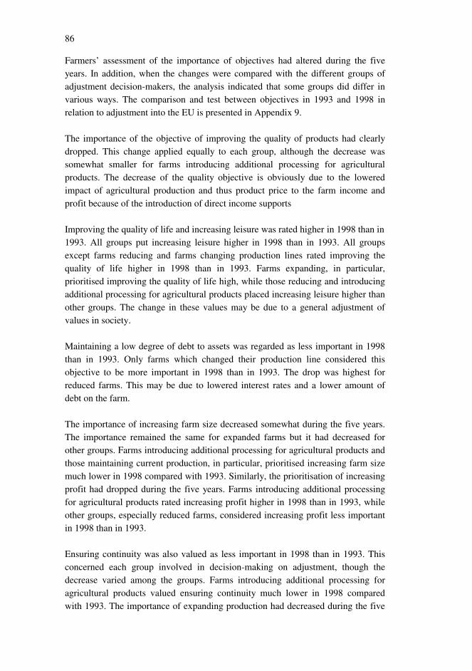
86

Farmers’ assessment of the importance of objectives had altered during the fiveyears. In addition, when the changes were compared with the different groups ofadjustment decision-makers, the analysis indicated that some groups did differ invarious ways. The comparison and test between objectives in 1993 and 1998 inrelation to adjustment into the EU is presented in Appendix 9.

The importance of the objective of improving the quality of products had clearlydropped. This change applied equally to each group, although the decrease wassomewhat smaller for farms introducing additional processing for agriculturalproducts. The decrease of the quality objective is obviously due to the loweredimpact of agricultural production and thus product price to the farm income andprofit because of the introduction of direct income supports

Improving the quality of life and increasing leisure was rated higher in 1998 than in1993. All groups put increasing leisure higher in 1998 than in 1993. All groupsexcept farms reducing and farms changing production lines rated improving thequality of life higher in 1998 than in 1993. Farms expanding, in particular,prioritised improving the quality of life high, while those reducing and introducingadditional processing for agricultural products placed increasing leisure higher thanother groups. The change in these values may be due to a general adjustment ofvalues in society.

Maintaining a low degree of debt to assets was regarded as less important in 1998than in 1993. Only farms which changed their production line considered thisobjective to be more important in 1998 than in 1993. The drop was highest forreduced farms. This may be due to lowered interest rates and a lower amount ofdebt on the farm.

The importance of increasing farm size decreased somewhat during the five years.The importance remained the same for expanded farms but it had decreased forother groups. Farms introducing additional processing for agricultural products andthose maintaining current production, in particular, prioritised increasing farm sizemuch lower in 1998 compared with 1993. Similarly, the prioritisation of increasingprofit had dropped during the five years. Farms introducing additional processingfor agricultural products rated increasing profit higher in 1998 than in 1993, whileother groups, especially reduced farms, considered increasing profit less importantin 1998 than in 1993.

Ensuring continuity was also valued as less important in 1998 than in 1993. Thisconcerned each group involved in decision-making on adjustment, though thedecrease varied among the groups. Farms introducing additional processing foragricultural products valued ensuring continuity much lower in 1998 comparedwith 1993. The importance of expanding production had decreased during the five

87

years as well. This concerned all groups except farms which changed theirproduction line.

Increasing total incomes was regarded as more important in 1998 than in 1993.This concerned all groups except reduced farms. Farms adding processing foragricultural products had altered the importance more than other groups. Increasingassets had decreased somewhat during the five years. As far as the groups involvedin adjustment to the EU were concerned, increasing assets was lower in 1998 thanin 1993 except among those farms reducing and changing their production line.

The importance of taking care of the environment had decreased slightly during thefive years. This concerned all other groups except those introducing additionalprocessing for agricultural products. The importance of ensuring liquidity decreasedsomewhat during the five years for all groups involved in adjustment to the EU.Improving return of capital was regarded as less important in 1998 than in 1993.This concerned all other groups except those increasing off-farm incomes.

Farms which had quit production during 1998-2000 differed in certain cases fromother farms as far as changes of objectives were concerned. Ensuring continuity,increasing profit, avoiding losses and maintaining a low degree of debt to assetswere rated lower in 1998 than in 1993 compared to the other groups.

Farmers assessed increasing profit as more important in 1993 than in 1998, whileincreasing total incomes was regarded as more important in 1998 than in 1993.However, in the principal component analysis, both of these objectives loaded tothe third principal component, increase returns, thus farmers regarded increasingprofit and increasing total incomes as similar. The reason behind this change isdifficult to explain and therefore requires further study.

The prioritisation of the most important values was quite stable during 1993-1998.The changes in values were somewhat smaller compared with the changes inobjectives. Values are more stable than objectives, and therefore they may explainlong-term, strategic decisions more than objectives. The most important valueswere independence of work, versatility of work, the possibility to do work onelikes, and lifestyle (Table 5.12). The comparison and test between values in relationto adjustment into the EU is presented in Appendix 10.

88

Table 5.12 Comparison of changes in values.Value Mean in

1998Mean in

1993Diffe-rence

Risk(p)

Lifestyle

Possibility to gain profit

Outdoor life

Independence of work

Respect derived from work

Entrepreneurship

Possibility to develop oneself

Belonging to a farm community

Environmentally friendly production

Job assurance

Challenge in work

Continuing family farm

Possibility to express oneself

Possibility to expand production

Possibility to earn reasonable incomes

Possibility to do work one likes

Versatility of work

4.91(1.25)

4.38(1.35)

4.48(1.33)

5.18(1.05)

4.18(1.49)

4.68(1.24)

4.45(1.20)

3.89(1.43)

4.54(1.19)

4.70(1.37)

4.66(1.25)

4.49(1.55)

4.66(1.19)

3.58(1.52)

4.87(1.20)

5.01(1.11)

5.05(1.06)

5.09(1.14)

4.42(1.39)

4.64(1.27)

5.42(0.93)

3.95(1.57)

4.87(1.24)

4.61(1.35)

3.85(1.49)

4.27(1.35)

4.75(1.41)

4.71(1.31)

4.67(1.44)

4.73(1.28)

3.85(1.53)

4.64(1.32)

5.09(1.13)

5.17(1.00)

-0.17(1.41)-0.04

(1.54)-0.15

(1.45)-0.25

(1.24)+0.20(1.70)-0.24

(1.45)-0.21

(1.47)+0.06(1.71)+0.32(1.43)-0.05

(1.51)-0.11

(1.46)-0.29

(1.49)-0.18

(1.35)-0.43

(1.67)+0.19(1.40)-0.12

(1.21)-0.15

(1.18)

0.026

0.646

0.056

0.000

0.031

0.002

0.008

0.526

0.000

0.566

0.180

0.000

0.015

0.000

0.013

0.018

0.022

Number of cases 367 in 1998 and 469 in 1993, scale from 1 to 6 (1=not important, 6=very important). Meansin 1998 and in 1993 are calculated with all cases. However, the difference between values in 1993 and in 1993is calculated in pairs, thus the distinction between mean in 1998 and mean in 1993 differs from the column‘difference’. Standard deviation is presented in parenthesis. T-test is used here as a standard measure tocompare values. To test the hypothesis that the 1998 and 1993 values have the same mean, the two-tailed test isused to calculate the p-values.

The value of environmental issues, the possibility to earn a reasonable income,respect derived from work and belonging to a farm community have increasedslightly during the five years, while the assessment of the other values was regardedas less important in 1998 than in 1993. The change in the environment value maybe because of increased awareness of environmental issues as well as obligations inagri-environmental support. Maintained farms, farms which introduced additionalprocessing for agricultural products and those increasing off-farm incomes valuedenvironmental issues higher in 1998 than in 1993.

Farms maintaining and expanding production rated the possibility to earn reason-able incomes higher in 1998 than in 1993, while those reducing and increasing off-farm incomes considered this value to be less important in 1998 than in 1993.

89

Farms which changed production lines valued respect derived from work higherthan other groups, while reduced farms clearly rated it lower. Farms maintainingproduction and those increasing off-farm incomes assessed the social value ofbelonging to a farm community as more important in 1998 than in 1993, whileother groups rated this value as less important in 1998.

Farms which introduced additional processing for agricultural products assessedchallenge in work, versatility of work, entrepreneurship, independence and thepossibility to express oneself higher in 1998 than in 1993, whereas other groupsrated these values lower. Reduced farms especially assessed these values muchlower in 1998. Thus, values connected to entrepreneurship had lowered in basicagricultural production, while they had risen in other types of enterprise.

The valuation of expanding in 1998 compared to 1993 was higher for farms whichchanged their production line and lower for other groups. Consequently, the changeof production line was based on improving profitability and expanding theproduction. The value of the possibility to gain profit was assessed lower in 1998than in 1993 by other groups except farms expanding and those changing theirproduction line. The value of continuing the family farm was lower in 1998 than in1993 among all groups. Reduced farms valued the possibility to do work one likesas more important in 1998 than in 1993, while other groups rated it lower.

As far as the significance of uncertainty factors was concerned, the changes inagricultural policy were regarded as more significant than earlier, while theuncertainty of sales of products was regarded as less important nowadays thanearlier on. Highlighting the uncertainty of agricultural policy was obviously due tothe high dependence of farms on direct supports and therefore on political deci-sions. On the other hand, sales of products may be regarded among farmers asbetter guaranteed in the EU than earlier on, and moreover, the impact of productsales on returns is smaller for the lowered producer prices in the EU. Farmers seemto take the changes in the operational environment into consideration whileassessing the uncertainty factors.

The share of risk averse farmers declined somewhat during the five years. In thequestion regarding risk, the average amount of willingness to pay had increasedFIM 2.2 (10%) during the five years. In addition, the change in attitudes toward riskhad altered in a dissimilar way among the various groups. Risk aversion hadincreased 10% among farms expanding, while in the other groups risk aversion waslower. Perceptually risk aversion had lowered most among reduced farms (43%),among farms increasing off-farm incomes (33%) and among farms introducingadditional processing for agricultural products (26%).

90

Some managerial issues had altered greatly between 1993-1998, whereas some hadremained quite stable. Utilisation of a computer in farm management had increasedsignificantly during the five years. This is mainly due to the development ofinformation technology in society. However, the use of time for planning andcontrol of production and economy stayed quite the same in 1998 compared to1993. Farms which increased off-farm incomes, in particular, had reduced thistime. Furthermore, the share of farms making a budget had risen only slightlyduring the five years. Farms which expanded, which maintained current productionand those increasing off-farm incomes had increased budget making, while farmsreducing production did less budget work in 1998 than in 1993.

91

6. Examination of the results and conclusions

The farmers’ adjustment into the EU according to this study was divided intofarmers who maintained production (44%), farmers who expanded production(20%), farmers who quit production (15%), farmers who increased off-farmincomes (10%), farmers who changed their production line (5%), farmers whoreduced production (3%), and farmers who introduced additional processing foragricultural products (3%). If the farms which quit are omitted, the share of farmerswho maintained their current production is over 50%. However, the group was nothomogenous, because some of them had made a conscious decision to maintaincurrent production while others in the group were clearly quite unsure about thefuture. This was linked to the question of a successor and could be observed by theintention to refrain from investments. Almost 20% of the farmers maintainingcurrent production were unsure about the adjustment and 10% of them planned toquit within the five years.

The reasons behind the solutions were severe, and about 75% of farmers declaredthat the decision was based on plans, calculations and assessments of variousalternatives. Öhlmer et. al. (1993, 53) noted that one reason why farmers do notmake detailed plans is uncertainty in the operational environment. According toCarson (1988, 93), long term decision-making and farm enterprise selection appearto be especially problematic for farmers.

The proposed adjustment strategy, being dependent on chosen strategy, wasdistributed to farmers maintaining production (37%), farmers expanding production(17%), undecided farmers (14%), farmers planning to quit production (8%),farmers increasing off-farm incomes (8%), farmers introducing additional process-ing for agricultural products (7%), farmers reducing production (4%), farmersplanning to hand over to the next generation (3%), and farmers changing produc-tion line (3%). Kuhmonen (1995, 4) surveyed the five-year plans of Finnish farmshaving at least five hectares of arable land in 1995. In his study the share of farmsplanning to quit during the succeeding five years was higher (21%), while the levelof farms planning to maintain current production (37%) was similar to this study. Inaddition, the share of farms planning to introduce additional processing foragricultural products was higher (11%), whereas the share of farms planning toexpand was lower (8%) than in this study. Ylätalo et. al. (1998b, 85) explained theintention of dairy farmers in the municipality of Vieremä to continue production forat least five years. In 1996, six percent of farmers intended to quit production.

In the follow-up study in 1996 Kuhmonen (1996, 61-62) found that the intention toquit had lowered to 17%, the number of uncertain farms had increased and the level

92

of farms planning to introduce additional processing for agricultural products haddecreased. In addition, during the three year period, 28% of farmers had alteredtheir plans (Kuhmonen 1996, 62). Also Ylätalo et. al. (1998b, 83-84) noticed thatquite a large number of farmers altered their plans during a one-year period.Because the intention does not always correspond to real behaviour, the reliabilityof intention variables is lower then those variables measuring already materialisedactions (Ajzen 1985).

Among bookkeeping farms the share of farms planning to quit during the five yearswas a bit lower (6%) but the share of farms planning to expand production wasclearly higher (39%) (Jokela and Ala-Orvola 1999). The greater share of expandingfarms is mainly due to the representativeness1 of bookkeeping farms in thepopulation.

The level of planned investments was lower than implemented investments andonly 70% of farmers planned to invest during the following five years. Accordingto Rytsä (1998, 27), the most important reasons to refrain from investments are riskand uncertainty related to the investment, adequate current levels of production andinadequate investment support. According to the farmers’ plans, especiallyinvestments in machinery and environmental investments were decreasing, whileinvestments for additional land increased slightly. The withdrawal or reduction ofinvestments and thus he giving up of the utilisation of technological developmentas a adjustment method may only work in the short term; according to Pehkonenand Mäkinen (1998), in the longer term this kind of behaviour leads to economicproblems and the stopping of production.

The preference of the most important objectives and values had not altered duringthe five years. The most important objectives were ensuring liquidity, avoidinglosses, taking care of the environment, improving the quality of life and reducingrisk. The findings are in agreement with those of Hahtola (1971), Smith andCapstick (1976), Harper and Eastman (1976) and Gasson and Errington (1993)where objectives related to risk management were also emphasised.

The most important values were independence of work, versatility of work, thepossibility to do work one likes, lifestyle and the possibility to earn reasonableincomes. The ranking is quite similar to the observations of Gasson’s (1973) andGillmor’s (1986) studies, where intrinsic values were preferred to instrumentalones. The results also confirmed Gasson’s (1973, 532) conclusion that smallerfarms consider intrinsic values as being more important than bigger farms.

1 Bookkeeping farms consist of about 1000, mainly full-time farms, whose average size is 40hectares.

93

The most significant uncertainty factors were changes in agricultural policy,maintaining liquidity, variations in product prices, accidents and outlets ofproducts. Compared with the studies of Patrick et. al. (1985), Meuwissen et. al.(1999) and Harwood et. al. (1999), Finnish farmers placed institutional andfinancial risk before production risk. This can be explained by the high level ofsupport and its connection to institutional decision-making. According to Hardakeret. al. (1997, 262) the government usually increases the complexity of the farmers’operational environment.

The most important risk management strategies were maintaining adequateliquidity and solvency, and planning and controlling production and the economy.Compared with the studies of Patrick et. al. (1985) and Meuwissen et. al. (1999),Finnish farmers emphasised financial strategies somewhat more than productionand marketing strategies. This may be due to the fact that before accession to theEU farmers were able to utilise only a limited number of production and marketingstrategies to reduce risk, and even if farmers nowadays are able to use severalproduction and marketing strategies, they may not be very familiar with them.

In this study, values and objectives seemed to be rather stable even when a bigchange has taken place in the operational environment. However, the drastic effectof the changeover from price support to direct income support depending onadministrative decisions is reflected in the changes of objectives and values offarmers. Values are in nature very permanent, so the five year time period is rathershort to observe the alteration of values. Nevertheless, even minor changes mayreflect the direction of change. According to Gasson and Errington (1993, 105),objectives are less stable than values. This was confirmed in this study as well.

The objective of improving the quality of products was clearly less prioritised aftermembership of the EU compared to before, and correspondingly, the valuesassociated with entrepreneurship were lower after joining the EU than before. Themajor reason behind this is the agricultural policy of the EU: direct income supportis tied to the number of hectares and animals instead of the number and quality ofagricultural products produced. Thus, the impact of entrepreneurship and quality ofthe economic result of the farm was greatly reduced after accession to the EU. TheAgenda 2000 reform further increased the relative importance of subsidies forfarmers’ economic results. Timonen (2000, 153-156) has shown that entrepreneur-ship is positively correlated to success in the farm business. Also Sipiläinen et. al.(1998, 161) suggested that the Agenda 2000 reform might diminish the motivationof farmers.

On the other hand, objectives relating to the quality of life and leisure had becamemore important during the five years. This may originate in the general alteration ofvalues in society which highlight quality and leisure in life. In addition, environ-

94

mental point of views seemed to be valued as more important with EU membershipthan before. This can be partly attributed to the farmers’ high level of involvementin the agri-environmental support programme. Tamminen (1997) also reported apositive change in farmers’ environmental attitudes.

In conclusion, in the light of this study, the agricultural policy of the EU may havereduced the value of entrepreneurship in the countryside and this can be noted inconcrete terms, for instance, in the assessment of the importance of quality inproduction. In the longer term, if the current agricultural policy continues alongsimilar lines, the value orientation of farmers may alter permanently.

The agricultural policy of the EU has been able to guarantee farmers a certainincome level, even though their economic results and profitability have beendecreasing within the EU (see Maatilatalouden yritys- ja tulotilasto 1998).However, one has to take into consideration the impact of change in farmers’values, objectives, attitudes and motivation when farmers’ income formations havealtered greatly. The agricultural policy of the EU tends to equalise farmers’economic results, because the quantity and quality of production have only partialinfluence on the economic result, while a great deal of the result is not tied to thesuccess of farming. Therefore, the current situation does not provide enoughincentives for farmers.

The current situation is not solely favourable for the consumer either; even if thepolicy is able to meet the objective of providing food for consumers at reasonableprices, consumers may have to compromise over the variety and quality of food,because the quality and variety of agricultural products are not objectives of theCAP (see Ritson 1997, 2). The BSE crises can be seen as the ultimate example ofthis. The magnitude of quality and safety in food production should be raised toinclude the quality aspect in the objectives of the CAP. In practice, to prevent thefurther decline in the motivation and entrepreneurship of farmers, the impact ofentrepreneurship should be raised by reducing the magnitude of income support tofarmers’ income, or by adjusting the current form of income supports to providemore incentives for farmers.

The uncertainty associated with institutional risk had increased within the EU,while the significance of market risk had lowered during the five years. Thediminished impact of production to farm income has decreased market risk, whilethe introduction of direct income support has increased institutional risk originatingfrom agricultural policy. The change in managerial practice was only minor exceptfor the increased utilisation of computers, which can be attributed to the commonevolution of information technology in society.

95

In this study, all the components of the operational model, the production andeconomic factors of the farm, the characteristics of the farmer, and the operationalenvironment had an influence on the farmers’ decision-making on adjustment intothe EU. The relative importance and magnitude of these factors greatly variedamong different types of farms and farmers. This could be verified in the statisticaltests complemented with the open questions in the questionnaire. In other words,farmers who utilised an alternative adjustment strategy for EU membership(maintaining current production, expanding current production, reducing currentproduction, changing production lines, introducing additional processing foragricultural products, increasing off-farm incomes, or quitting) had differentobjectives, values, personalities as well as cognitive styles, their farms differed inrelation to variety of production and economic factors, and they valued thesignificance of uncertainty factors differently.

The farm-related factors may limit or direct the alternative choices farmers have instrategic decision situations even in the longer term. Farmers have to take currentproduction and economic factors, development possibilities and changes in theoperational environment into account in their decision processes. Correspondingly,farmer-related issues may limit or offer new possibilities in strategic decision-making, Taking the strengths and weaknesses of the individual farm and farmerinto account, farmers worked out their solutions based on the threats and possibili-ties within the environment. Thus, farmers seemed to take into consideration theelements presented in a strategic management study (see Porter 1998a and 1998b).

The size of the farm, as measured by the amount of arable area, number of animalsand on-farm incomes; type of production, as measured by the main production line;and the economic situation of farm, as measured by the agricultural income anddebt, affected the strategic decision-making of farmers. The farmers’ basiceducation also had an influence on decisions. For example, the education of thefarmer or his/her spouse affects the possibility of obtaining or increasing off-farmincomes, or the option to quit farming before retirement age.

The age of farmer and correspondingly the life cycle of the farm seem to beimportant factors when explaining the adjustment into the EU and is thus relevantto strategic decision-making. Most of the farms in Finland are family-farms, whoselife cycle is connected to the life cycle and age of farmers. In the early phase, thefarm is often developed and expanded, while at the exit stage, production ismaintained or even declines. Such results have been reported by Potter and Lobley(1996) as well as Ylätalo et. al. (1998a, p. 168). Assurance of a successor may havemore influence upon objectives and farm performance than the farmer’s age(Gasson and Errington 1993, 96). Boehlje and Eidman (1984) as well as Carson(1988) suggested that the life cycle of the farm is an important element in farmmanagement.

96

In this study, the assurance of a successor affected future decisions especiallyamong the biggest group of farmers, farmers who had decided to maintain currentproduction; the greater the assurance, the more certain these farmers were aboutfuture decisions. If a farmer has a successor, the future direction and continuity ofthe farm is better secured in the long term, and this is an important factor affectingthe motivation of farmers to continue production and develop the farm. Farmshaving no successor tended to develop the farm and invest in it less than thosefarms, which had a successor assured. This kind of behaviour was also noted byPotter and Lobley (1992), who found that elderly farmers without successors hadlittle incentive to expand, invest capital or even maintain production.

Uncertainty proved to be one of the key issues which influenced generation shifts.Thus, introducing institutional measures to reduce risk in farm management may bea more effective way to utilise a successful structural policy than by for instanceusing traditional measures of structural support. Farmers regarded institutional riskas the most significant factor causing uncertainty, so practising long-term,consistent support and structural policy reduces institutional risk and thereforeaffects the level of shifts from one generation to the next.

The results regarding attitudes toward risk in this study confirmed earlier outcomes(for instance Dillon and Scandizzo 1979; Meuwissen et. al. 1999) that the majorityof farmers are risk averse. Attitudes towards risk have diminished during the fiveyears in each group except amongst the expanded farms. Risk aversion had fallenmost among reduced farms, among farms which increased off-farm incomes andamong farms introducing additional processing for agricultural products. Expandedfarms have invested more than other groups in basic agriculture and their familyincome is more dependent on farm income than other groups. Thus, the decision toexpand combined with the big change in the operational environment led to higherrisk aversion for the farmers who had expanded, while risk aversion decreased inother groups.

Even though the validity of the variable for measuring farmers’ attitudes towardrisk was not adequate, it seems that if the relative significance of agriculturalproduction diminishes in family-farm life (diversification of the family’s work andinput outside traditional agriculture), risk aversion decreases. If investments andinputs in agricultural production increase, then the farmers’ risk aversion will alsoincrease. Thus, farm management is regarded as a risky business and this may beobserved from the risk attitude behaviour of the farmers. Farmers who haveexpanded production may also be more familiar with the concept of risk than otherfarmers, because they have faced the risks when they made the decision to expand.This result is similar to that of Meuwissen et. al. (1999), where more risk aversefarmers had larger farms. Correspondingly, Maikki and Somwaru (2001) observed

97

that higher risk farmers behaved in a more risk averse way than the average farmerwhen selecting yield and crop insurance.

The objective of developing the farm and production and the values of earning, thefarming lifestyle, meaningful work and entrepreneurship in the countryside alsoseemed to be important factors when explaining the decision-making. Prioritisationof other objectives rather than developing did not differ significantly in relation tothe adjustment decisions. The relative importance of the farmers’ value orientationprobably increases in the decision-making when the strategic and significantdecisions problems are more long term. This is especially evident in family-farmswhere these decisions affect the whole family. Thus in strategic decisions aspectsother than economic ones are involved in the decision-making, and their role maybe emphasised or dominated if the problem is not easily structured, quantified, orassessed. For example, the decision to quit farming usually means that the farmergives up the farming lifestyle and sometimes living in the countryside. This reasonand the difficulty to find a substitute source of income in the countryside may beone reason behind why the actual decision to quit farming has been lower than theintention to quit farming according to several studies (see for instance Kuhmonen1996; Kallinen and Heikkilä 1998; Ylätalo et. al. 1998a).

Correspondingly, except for life cycle, the farmers’ valuation of entrepreneurshipand earning as well as prioritisation of development explains why a particulargroup of farmers are developing their farms within the EU’s operational environ-ment while the majority of farmers have decided to maintain, reduce or quitproduction. Expanded farms seemed to be economically oriented with the aim ofgaining profit and achieving profitable production by developing and expandingproduction. They regarded farming more as a business to be developed to gainprofit than a lifestyle in order to maintain farming and to live in the countryside.Gasson and Errington (1993, 100) noted also that the preference of values altersaccording to the size of the farm business; intrinsic values were regarded as moreimportant on smaller farms, while larger farms preferred instrumental and expres-sive aspects. The valuation of intrinsic values was highest among farmers who wereabout to quit production. Thus, the farmers’ objectives and values in farming andthe farm family explain to a considerable degree why certain decisions are taken onthe farm.

Farmers who quit production were older, less educated, and utilised fewer modernmanagement practices than the average farmer. Farmers who quit prioritised theobjective of expanding and continuing production as well as reducing risk lowerthan other farmers, and assessed instrumental and expressive values as low butintrinsic values as high. The size and income of farms which had quit weresomewhat smaller than average farms. The share of dairy and other crops farms washigher among farms which had quit than in the population. Pyykkönen (1999) also

98

concluded that the majority of farms which had quit had smaller incomes thanfarms on average. Kuhmonen (1996) as well as Keränen and Rytkönen (1996)noted that farms intending to quit were smaller in size than farms on average, andthat the probability of quitting farming was higher for older farmers. Similarconclusions were also reached by Ylätalo et. al. (1998b, 86). They (1998b, p. 85)discovered that the majority of farmers who quit decided to retire after farming.

Age, life cycle and education did, however, only partly explain the decision to quitfarming, because the age, life cycle and education of farmers who intended to quitproduction were quite average. In this study, the other explanatory factors for thedecision to quit farming were the objective of developing the farm and productionas well as the value of meaningful work.

The results of this study indicate that mere objectives, values, personality andcognitive style are not enough to explain the farmers’ adjustment into the EU andtherefore strategic decision-making. Correspondingly, the production and economiccharacteristics of farms do not explain farmers’ strategic decision-making. Neitherdoes the operational environment and changes to it explain their strategic decision-making. It is the combination and interaction of these factors that determines thestrategic decision-making of farmers, though the magnitude of various factors andinteraction between them varies in different contexts of decision-making and arealways dependent upon the situation of the individual farmer and farm.

The diversity of the factors affecting farmers’ decision-making complicates theunderstanding and prediction of their behaviour in strategic, long-term decision-making. Most of the farmer-related factors especially are qualitative and difficult tomeasure in a valid way. Gasson (1973) as well as Ruble and Cosier (1990) havealso noted that individual characteristics of decision-makers in various decisionsituations produce different outcomes. Thus, farmers’ decision-making is not easilyexamined using, for example, econometric models to predict changes and develop-ment in the agricultural structure. This can partly explain why these models fail topredict a farmers’ economic behaviour especially in longer term situations.However, this study does indicates that these factors should be taken into account.The result does adhere to that of Gasson and Errington (1993, 112), who arguedthat the logic of decision-making for family-farms is more complex than for othertypes of farms. The magnitude of farmer-related, psychological factors in thedecision-making is also stated by Willock et. al. (1999). As far as the theoreticalapproaches to decision-making are concerned, the results supported best the viewsof bounder rationality (Simon 1979) and the decision maker as an individual(Gasson 1973).

During the last decades the nature of farm-families has been evolving from thetraditional farm-family, where each member of the family works on the farm, to

99

various other types of farm-families which have a diversity of solutions to apply toagriculture. The share of agricultural income of a farmers’ total income has greatlydecreased during the last decade (Väre 2000). According to Peltola (2000), thephenomenon of pluriactivity of farm-families is on the increase; in his study 56% offarms were pluriactive and 44% were full-time farms. The continuously alteringoperational environment which provides opportunities and threats as well as adiversity of factors affecting the farmers’ decision-making indicates that thedifferentiation of farm-families in accordance with their adjustment strategy is alsoon the increase. Therefore, political macro level measures and instruments to guideFinnish agriculture and rural areas should be based on the same kind of strategy thatfarmers have chosen on a micro level, and should be as diverse and flexible aspossible in order to meet the various solutions that farmers have chosen. Otherwisepolitical level rural strategies only partly correspond to the farmers’ objectives andrequirements.

Family-farms especially consider adjustment at a family level instead of only a farmlevel. Therefore, the farm-family point of view should be underlined in addition tothe farm business point of view in agricultural policy. Harper and Eastman (1980,745-746) noted that farm goals may conflict with family goals in some cases, andthat the family instead of the farm enterprise is the relevant unit of analysis. Fennell(1982, 34-35) has noted that the likelihood of having succession for a farm isaffected both by the economic situation of the farm and the possibility to earn asatisfactory living outside farming. Thus, the question of the level of shift to thenext generation is a matter of agricultural, rural and regional policy.

The interpretation of the results should be done in a qualified way. The relativelylow response rate in the 1993 survey restricts the generalisation of the results eventhough the response rate was high in the 1998 follow-up survey. In addition, due tothe restriction of the sample to somewhat larger than average farms in 1993, theresults cannot be directly generalised for active farms and farmers. Taking thesefactors into consideration, the results of the study may be generalised as activefarms, which are somewhat larger in size than average farms in Finland, and tofarmers who are better educated than average farmers.

The validity of the variables which demanded the farmers’ assessment was lessthan the validity of other variables, even though the validity was enhanced byemploying several variables measuring the same issue and the individual variablesof objectives and values were combined to improve the validity of the measure-ment. The subjective component within the multivariate methods might also lowerthe validity of the results.

The survey methodology employed in this study did not allow control of theresponse situation, so it is not evident what farmers actually meant when they were

100

assessing the importance of objectives and values. For instance, the possibility thatsome farmers have paid sequential attention to goals (see, for instance, Simon1979) and some have not lowers the validity of the measurement and might affectthe results and conclusions. Similarly, the different cognitive styles of farmers mayhave an influence on the assessment of objectives and values. Öhlmer et. al. (1993,52) have reported the difficulty in directly observing the cognitive processes offarmers. Korhonen et. al. (1990, 177 ) noted that the form of presentation can affectthe decision-makers’ processing strategy. The decision-makers may act in a varietyof ways if they have different perceptions of the decision situation due to unequalaccess to information or varying interpretations of it (Casson 1982).

The direction of the influence between decision-making in the EU and values orobjectives was not fully evident in all cases. The independent variable, adjustmentinto the EU, was measured only once in 1998, while dependent variables weremeasured twice: in 1993 and in 1998. Thus, it was not possible to conclude fromthe available data, which variable had changed first but the argument was made ona theoretical basis. Objectives and values directly or indirectly influence thedecision-making, although in some cases in the longer term the direction ofinfluence can be the other way around as well. The latter direction, however, is notso obvious and the values especially can be regarded as very stable. The stability ofvalues and objectives in this study could also be verified by the rather minorchanges in objectives and values between 1993 and 1998.

The continuous change and increased level of uncertainty in the farmers’ opera-tional environment seems to be a permanent phenomenon at least for the nearfuture. The studies of Kallio (1997) and Mäkinen (1999) indicate that the changesin the operational environment of the EU have increased stress for farmers. Thesurveys in this study were carried out during periods of this kind of uncertainoperational environment. Thus, the validity and generalisation of the results due tothe changes in the operational environment may be considered to be adequate.

101

7. Summary

Finland’s accession to the European Union (EU) at the beginning of 1995 without atransitional period was one of the biggest changes for the Finnish agriculturalsector, and therefore for farmers. The new operational environment of the EUrequired farmers either consciously or unconsciously to make decisions concerningadjustment into the EU. Their decisions on adjustment may be classified intomaintaining farms, expanding farms, reducing farms, farms changing the produc-tion line, farms introducing additional processing for agricultural products, farmsincreasing off-farm incomes and quitting production.

This study aimed at explaining farmers’ decision-making on adjustment into theEU, and examining changes in their objectives, values, attitudes toward risk,managerial issues, and the significance of risk factors in the changing operationalenvironment. The theoretical model of farmers’ strategic decision-making, based onthe theory of risk, uncertainty and decision-making as well as previous studies, wasintroduced and operationalised by their decision-making. The model consisted ofproduction and economic factors of the farm, farmer-related factors, the operationalenvironment and decision-making.

The empirical data for the study consisted of three sets of data. A postal survey in1993 was conducted for active Finnish farmers with at least 10 hectares of arableland. In 1998, a follow-up survey was carried out for the same set of farmers whoresponded to the 1993 survey. Altogether 415 farmers responded to both surveys.These two data sets were complemented and validated by the data received fromthe rural business register. Several statistical tests were applied to test the opera-tional model.

Almost half of the farmers had maintained current production, one fifth hadexpanded production and 15% had quit production. The tests indicated that theproduction and economic factors of the farm, characteristics of the farmer and theoperational environment affected decision-making on adjustment into the EU. Themagnitude and interaction of these factors seemed to vary from one farm andfarmer to another. This was also confirmed by an open question, where farmersstated the major factors behind their solutions to adjustment. The assurance of asuccessor in family-farms affected farmers’ decision-making because strategicdecisions usually extend to the next generation. It was found that farmers’ objec-tives related to development and risk management as well as their value orientationwhich partly explained why farmers’ committed in different ways when makingdecisions on adjustment to the EU. The importance of values in decision-makingseems to increase the more long-term, strategic and significant the problems are.

102

The most important objectives and values had remained same during the five-yearperiod. The most important objectives were those associated with risk managementand the most important values were intrinsic values, like independence, versatilityof work and the possibility to do work one likes. However, farmers’ objectives andvalues had altered somewhat upon joining the EU compared with the time beforemembership. Values associated with entrepreneurship and the objective ofimproving the quality of products had been less prioritised, while objectives relatedto the quality of life and leisure as well as environmental issues had been prioritisedhigher in the operational environment of the EU. These changes were quite similarfor each group making decisions on adjustment. The major reason behind thesechanges was the introduction of the EU common agricultural policy (CAP), whichgreatly altered the farmers’ operational environment between 1993 and 1998.

Risk aversion had lowered in each group of decision-makers except amongexpanding farms, where risk aversion had increased. Changes in managerial issueswere minor except for the utilisation of computers, which had increased greatlyduring the five years. The significance of institutional risk had increased, whilemarket risk was regarded as less important to farmers now in the EU than beforemembership.

103

Selostus: Maatilayrittäjien EU-sopeutumiseen liittyvä

päätöksenteko

Riski ja epävarmuus ovat lisääntyneet suuresti Suomen maataloudessa 1990-luvulla. Epävarmuus oli suurimmillaan ennen Suomen liittymistä EuroopanUnioniin (EU), koska etukäteen oli tiedossa, että liittyminen vaikuttaisi suurestiSuomen maatalouteen ja maatilayrityksiin. Suomen liittyminen EU:hun vuoden1995 alussa ilman siirtymäaikaa on suurimpia yksittäisiä muutoksia, jotka ovatkohdistuneet Suomen maatalouteen ja sitä kautta yksittäisiin maatilayrityksiin.Suomen maatalouden siirtyminen osaksi EU:n maatalouspolitiikkaa laskimerkittävästi maataloustuotteiden tuottajahintoja ja lisäsi tuotteiden hintavaihtelua.Tuottajahintojen alentamisesta aiheutuvat tulonmenetykset pyrittiin korvaamaanmaatilayrittäjille erilaisilla sopeuttamistoimenpiteillä, joista suorat EU-tuet jakansalliset tuet ovat merkittävimpiä. Suorilla tuilla ei kuitenkaan kyetty kokonaankompensoimaan tuottajahintojen laskusta aiheutuvaa tulonmenetystä. Vuoden 2000alussa voimaan tullut Agenda 2000 lisäsi edelleen suorien tukien merkitystämaatilayrittäjien tulonmuodostuksessa. Kaikkiaan EU:n tuoma muutos maatilayrit-täjien toimintaympäristöön on lisännyt huomattavasti institutionaalista riskiämaataloudessa.

Muuttuneessa toimintaympäristössä maatilayrittäjien oli ratkaistava maatilayrityk-sensä sopeutuminen joko tietoisesti tai tiedostamatta. Vaihtoehtoina ovat nykyisentuotannon ylläpitäminen, tuotannon laajentaminen, tuotannon vähentäminen,tuotantosuunnan vaihtaminen, sivu- ja liitännäiselinkeinojen tai jatkojalostuksenkehittäminen, maatalouden ulkopuolisten tulojen lisääminen tai tuotannonlopettaminen. Päätös on strateginen ja hyvin kriittinen tilalle sekä viljelijäperheelle.Tämänkaltaisessa päätöstilanteessa yksinomaan voiton maksimointiin perustuvatpäätösmallit ovat riittämättömiä selittämään maatilayrittäjien päätöksiä.

Tutkimuksen tavoitteena on selittää, mitkä tekijät vaikuttavat maatilayrittäjien EU-sopeuttamispäätökseen. Toisena tavoitteena on tarkastella miten muuttuvatoimintaympäristö on vaikuttanut maatilayrittäjien tavoitteisiin, arvoihin,suhtautumiseen riskiin, liikkeenjohdollisiin tekijöihin sekä arviointiin eririskitekijöiden merkittävyydestä. EU-sopeuttamispäätöksenteko yleistetäänkoskemaan maatilayrittäjien strategista päätöksentekoa.

Tutkimuksen teoreettinen malli perustuu teoriaan riskistä, epävarmuudesta japäätöksenteosta sekä aikaisempiin tutkimuksiin. Malli koostuu maatilayrityksentuotannollista ja taloudellisista tekijöistä, maatilayrittäjästä päätöksentekijänä,päätöksenteosta sekä toimintaympäristöstä. Malli operationalisoidaan maatilayrit-täjien EU-sopeuttamispäätöksenteoksi.

104

Tutkimuksen empiirinen aineisto koostuu kolmesta osasta. Perustana on vuonna1993 vähintään 10 hehtaarin aktiivitiloille osoitettu postikysely, johon vastasi 547tilaa vastausprosentin ollessa 45. Kyseiselle tiloille suoritettiin vuonna 1998jatkokysely, johon 415 tilaa vastasi, jolloin vuoden 1998 kyselyn vastausprosentiksimuodostui 89%. Aineistoa täydennettiin ja sitä validoitiin maaseutuelinkeinorekis-terin tiedoilla.

Aineiston tavoite- ja arvomuuttujille suoritettiin pääkomponenttianalyysi jaanalyysissa saadut uudet muuttujat analysoitiin ja nimettiin. EU-sopeuttamispäätöksenteko-muuttujan suhdetta maatilayritystä, maatilayrittäjää ja

toimintaympäristöä mittaaviin muuttujiin testattiin F- ja χ2-testeillä. Maatilayrittäji-en tavoitteisiin, arvoihin, suhtautumiseen riskiin, liikkeenjohdollisiin tekijöihinsekä arviointiin eri riskitekijöiden merkitsevyydestä liittyviä muutoksia selvitettiint-testillä.

Tässä tutkimuksessa maatilayrittäjien EU-sopeuttamispäätös jakaantui nykyisentuotannon ylläpitäjiin (44%), tuotannon laajentajiin (20%), tuotannon lopettaneisiin(15%), maatalouden ulkopuolisia tuloja lisänneisiin (10%), tuotantosuunnanvaihtaneisiin (5%), tuotannon vähentäjiin (3%) ja sivu- ja liitännäiselinkeinoja taijatkojalostusta kehittäneisiin (3%). Tuotannon ylläpitäjistä osa ei ollut vielä tehnytlopullista ratkaisua vaan oli epävarma tilan tulevaisuudesta. Tämä oli yhteydessäepävarmuuteen tilan jatkajasta ja havaittavissa pidättäytymisaikomuksena tulevistainvestoinneista.

Tavoitteiden ja arvojen tärkeysjärjestys ei ollut juurikaan muuttunut viiden vuodenaikana. Tärkeimmät tavoitteet olivat riskinhallintaan liittyviä tavoitteita jatärkeimmät arvot olivat maatilayrittämisen perusluonteeseen liittyvä arvoja, kutentyön itsenäisyys, monipuolisuus ja mahdollisuus tehdä haluamaansa työtä. Sensijaan institutionaalisen riskin merkitys oli korostunut, kun taas markkinariskinmerkitys oli pienentynyt viiden vuoden kuluessa. Riskin karttaminen oli vähentynytviiden vuoden kuluessa kaikilla muilla ryhmillä paitsi laajentaneilla. Liikkeenjoh-dollisissa tekijöissä ei ollut tapahtunut merkittäviä muutoksia lukuun ottamattatietokoneen hyväksikäytön huomattavaa kasvua maatilayrityksissä.

Huolimatta siitä, että tavoitteiden ja arvojen priorisointi ei ollut suuresti muuttunut,voitiin havaita toimintaympäristön suuresta muutoksesta aiheutuvia muutoksia.Yrittäjyyteen liittyvien arvojen arvostus oli laskenut EU:ssa ja vastaavastituotteiden laadunparantamiseen liittyvien tavoitteiden merkitys oli selvästipienentynyt. Sen sijaan elämänlaatua ja vapaa-aikaa korostettiin enemmän 1998kuin 1993. Myös ympäristönhoitoon liittyvien asioiden arvostus oli lisääntynyt EU-aikana. Nämä muutokset olivat samansuuntaisia kaikissa EU-sopeuttamispäätöksentekoryhmissä.

105

Tutkimuksessa todettiin, että vaikka EU:n maatalouspolitiikka on jossain määrinkyennyt huolehtimaan maatilayrittäjien tulotasosta, ei tulonmuodostuksessatapahtuneen suuren muutoksen vaikutusta maatilayrittäjien arvoihin, tavoitteisiin,asenteisiin ja motivaatioon ole otettu huomioon. Nykyinen maatalouspolitiikkatasapuolistaa maatilayrittäjien tuloksia. Tuotannon määrällä ja laadulla on vainosittainen vaikutus tulokseen suuren osan tuloista tullessa riippumatta siitä, mitenhyvin maatilayrittämisessä onnistutaan. Maataloustuotteiden laadun ja turvallisuu-den merkitystä tulisikin korostaa ottamalla ne mukaan osaksi EU:n maatalouspoli-tiikan tavoitteita. Jotta maatilayrittäjien yrittäjyyden ja motivaation lasku voitaisiinkäytännössä pysäyttää, tulisi suoran tulotuen osuutta viljelijän tulomuodostuksessapienentää tai muuttaa tulotukien nykyistä muotoa sellaiseksi, joka kannustaisimaatilayrittäjiä nykyistä enemmän.

EU-sopeuttamispäätöksen todettiin olevan yhteydessä maatilayrityksen tuotannolli-seen ja taloudelliseen tilanteeseen, maatilayrittäjän ominaisuuksiin ja toimintaym-päristön muutoksiin. Näiden eri tekijöiden tärkeys ja suhteellinen merkitys vaihtelisuuresti maatilayrityksestä ja maatilayrittäjästä riippuen. Tämä seikka voitiin myöstodeta avoimella kysymyksellä, jossa maatilayrittäjiltä tiedusteltiin tärkeimpiä syitäsopeuttamispäätökseen. Varmuus jatkajasta perheviljelmissä vaikutti maatilayrittä-jien päätöksentekoon, koska strategiset päätökset yleensä kohdistuvat seuraavillesukupolville asti. Tiloilla, joilla ei ollut jatkajaa tiedossa, oli alhaisempi kehittämis-ja investointihalukkuus ja tulevaisuus nähtiin epävarmempana kuin tiloilla, joillaoli jatkaja tiedossa. Koska jatkamishalukkuus on yhteydessä epävarmuuteentoimintaympäristössä, ja koska maatilayrittäjät pitivät institutionaalista riskiämerkittävimpänä epävarmuustekijänä, pystyisi valtiovalta parhaiten edistämäänsukupolvenvaihdoksia toimenpiteillä, jotka vähentävät institutionaalista,maatalouspolitiikasta aiheutuvaa riskiä.

Tutkimuksessa havaittiin, että maatilayrittäjien kehittämiseen ja riskinhallintaanliittyvät tavoitteet sekä arvot selittivät osin sen, miksi maatilayrittäjät tekiväterilaisia EU-sopeutumisratkaisuja. Arvojen merkitys päätöksenteossa vaikuttaisikasvavan mitä strategisemmasta ja merkittävämmästä sekä mitä pidemmänaikavälin päätösongelmasta on kysymys. Täten maatilayrittäjien strategistapäätöksentekoa ei voida selittää yksinomaan maatilayrityksen liittyvillä taloudelli-silla ja tuotannollisilla tekijöillä vaan myös maatilayrittäjään ja maatilaperheeseenliittyvät tekijät tulee huomioon ottaa.

Tulosten yleistettävyyteen koskemaan kaikkia Suomen maatilayrityksiä jamaatilayrittäjiä tulee suhtautua varauksellisesti. Kyselyn suuntaaminen keskimää-räistä suuremmille tiloille ja vuoden 1993 kyselyn suhteellisen alhaisen vastauspro-sentin vuoksi tulokset voidaan yleistää hieman keskimääräistä suurempiin tiloihinja keskimääristä paremmin koulutettuihin maatilayrittäjiin. Myös vastaajan arviota

106

vaativien kysymysten validiteettiin sekä monimuuttujamenetelmien tuloksiinmenetelmiin liittyvän subjektiivisuuden vuosi tulee suhtautua varauksella.

107

References

Agenda 2000 - Agriculture. European Commission.

Ajzen, I. 1985. From intentions to actions: a theory of planned behaviour. Actioncontrol: from cognition to behaviour, 11-39 (edited by Kuhl, J. &Beckmann, J.).

Ala-Orvola, L. 1997. Aktiiviviljelijöiden tuotantoon ja toimentuloon liittyvätsuunnitelmat vuoteen 2001. Maatalouden taloudellisen tutkimuslaitok-sen selvityksiä 12/97.

Allais, M. 1953. Le comportement de l’homme rationnell devart de risque:Critique des postulats et axiomes de l’ecole Americaine. Econometrica21, 503-546.

Allardt, E. 1976. Hyvinvoinnin ulottuvuuksia. WSOY, Porvoo.

Allison, G.T. 1971. Essence of Decision. Boston: Little, Brown.

Anderson, J.R., Dillon, J.L. & Hardaker, J.B. 1977. Agricultural Decision Analy-sis. Ames. Iowa.

Andersson, H. & Bengtsson, B-A. 1993: Expectation Formulation among NordicAgricultural Producers - An Outline for Joint Nordic Research. TheNordic Research Program for Risk Management in Agriculture. Pre-liminary report. 17-36.

Artto, E., Koskela, M. & Leppiniemi, J. 1989. Ulkoisen ja sisäisen laskentatoimenperusteet ja hyväksikäyttö. Gaudeamus.

Biswanger, H.P. 1980. Attitudes toward Risk: Experimental Measurement inRural India. American Journal of Agricultural Economics 63(3), 395-407.

Blaug, M. 1992. The Methodology of Economics or how economists explain.Cambridge University press. Second Edition.

Boehlje, M.D. & Trede, L.D. 1977. Risk management in agriculture. Journal of theAmerican society of farm managers and rural appraises 41(1), 20-28.

Boehlje, M.D. & Eidman, V.R. 1984. Farm management. John Wiley & Sons.

Boland, L.A. 1981. On the Futility of Criticizing the Neoclassical MaximizationHypothesis. American Economic Review 71(5), 1031-1036.

108

Brandes, W. 1989. On the limitations of armchair economics: Some views of anarmchair agricultural economist. European Review of AgriculturalEconomics 16(1989), 319-343.

Bray, J.H. & Maxwell, S.E. 1985. Multivariate Analysis of Variance. Sage Publi-cations.

Carlson, J.E. 1988. Farmers’ Perceptions about the Management of their Farms.Journal of the American Society of Farm Managers and Rural Ap-praisers 58(1), 91-96.

Carmines, E.G. & Zeller, R.A. 1979. Reliability and Validity Assessment. SagePublications.

Casson, M. 1982. The Entrepreneur: An Economic Theory. Martin Robertson.

Castle, E.N., Becker, M.H. & Nelson, G.A. 1987. Farm Business Management.The Decision-Making Process. 3. edition. Macmillan Publishing Com-pany, New York.

Chatfiled, C. & Collins, A. 1980. Introduction to Multivariate Analysis. Chapmanand Hall, New York.

Chiang, A.C. 1984. Fundamental Methods of Mathematical Economics. 3. edition.McGraw-Hill.

Chou, Y. 1989. Statistical Analysis for Business and Economics. Elsevier SciencePublishing.

Churchman C.W., Ackoff R.L. & Arnoff E.L. 1957. Introduction to OperationsResearch. John Wiley & Sons, New York.

Colson, G. 1985. Theories of Risk and MCDM. Multiple Criteria DecisionMethods and Applications, 171-196 (edited by Fandel, G. & Spronk,J.). Springer-Verlag.

Copeland, T.E. & Weston, J.F. 1988. Financial Theory and Corporate Policy. 3.edition. Addison-Wesley.

Cyert, R.M. & March, J.G. 1963. A Behavioral Theory of the Firm. New York.

Dillon, J.L. & Scandicco, P.L. 1978. Risk Attitudes of Subsistence Farmers inNortheast Brazil: A Sampling Approach. American Journal of Agri-cultural Economics 60(3), 425-435.

Drucker, P.F. 1974. Management: Tasks, Responsibilities, Practices. Harper &Row, New York.

109

Dyer, J.S., Fishburn, P.C., Steuer, R.E., Wallenius, J. & Zionts, S. 1992. Multiplecriteria decision making, Multiattribute utility theory: the next tenyears. Management Science 38(5), 645-654.

Einhorn, H. J. & Hogarth, R.M. 1987. Decision Making under Ambiguity. Ra-tional Choice. The Contrast between Economics and Psychology, 41-66 (edited by Hogarth, P.J. & Reder, M.W.). The University of Chi-cago Press.

Eppen, G.D., Gould, F.J. & Schmidt, C. 1988. Quantitative concepts for manage-ment. Decision making without algorithms. 3. edition. Prentice-Hall,Inc.

Fennell, R. 1981. Farm succession in the European Community. SociologiaRuralis 21, 19-41.

Finnish Agriculture and Rural Industries 1998. Agricultural Economics ResearchInstitute Publications 91a.

Fishburn, P.C. 1989. Foundations of Decision Analysis: Along the Way. Manage-ment Science 35(4), 387-405.

Fleisher, B. 1990. Agricultural Risk Management. Lynne Rienner Publishers.Boulder & London.

Fowler, F.J. 1990. Survey Research Methods. 8. edition. Sage Publications.

Friedman, M. 1962. Price Theory: A Provisional Text. Aldine, Chicago.

Gabriel, S.C. & Baker, C.B. 1980. Concepts of Business and Financial Risk.American Journal of Agricultural Economics 62(3), 560-564.

Gasson, R. 1973. Goals and values of farmers. Journal of Agricultural Economics24(3), 521-537.

Gasson, R. & Errington, A. 1993. The Farm Family Business. CAB International.

Giles, T. & Renborg, U. 1990. Farm Management: What's it all about? FarmManagement 7(8), 399-411.

Giles, T. & Stansfield, M. 1990. The Farmer as a Manager. 2. edition. CABInternational.

Gillmor, D.A. 1986. Behavioural Studies in Agriculture: Goals, Values andEnterprise Choice. Ir. J. agric. Econ. rur. Sociol. 11, 19-33.

Gul, F.A. 1984. The Joint and Moderating Role of Personality and Cognitive Styleon Decision Making. The Accounting Review 59(2), 264-277.

110

Hahtola, K. 1971. Forest owner's decision making and theories of the firm.Seloste: Metsänomistajan päätöksenteko ja yrityksen teoriat. Työteho-seuran julkaisuja 158

Hamilton, J.E. & Bryant, W.R. 1965. Profitable Farm Management. Prentice Hall.

Hardaker, J.B. & Huirne, R.B.M & Anderson, J.R. 1997. Coping with Risk inAgriculture. CAB International.

Harper, H.W. & Eastman C. 1980. An Evaluation of Goal Hierarchies for SmallFarm Operations. American Journal of Agricultural Economics 62(4),742-747.

Harwood, J., Heifner, R., Coble, K., Perry, J. & Agapi, S. 1999. Managing Risk inFarming: Concepts, Research, and Analysis. U.S. Department of Agri-cultural Economics Report 774.

Hazell, P.B.R. 1982. Application of Risk Preference Estimates in Firm-Householdand Agricultural Sector Models. American Journal of AgriculturalEconomics 64(2), 384-390.

Hertz, D.B. & Thomas, H. 1983. Risk Analysis and its Applications. John Wiley& Sons.

Hirsjärvi, S. & Hurme, H. 1979. Teemahaastattelu. Gaudeamus.

Hirvonen, A. 2000. Maatalouden kokonaislaskelmat 1992-2000. Maataloudentaloudellisen tutkimuslaitoksen tutkimuksia 244, 104-148.

Hodgson, G. 1985. The Rationalist Conception of Action. Journal of EconomicIssues 19(4), 825-851.

Hofer, C.W. & Schendel, D. 1978. Strategy Formulation: Analytical Concepts.West Publishing Company.

Hogarth, R.M. 1980. Judgement and Choice. The Psychology of Decision. JohnWiley & Sons.

Hogarth, R.M. & Reder, M.W. 1987. Introduction: Perspectives from Economicsand Psychology. Rational Choice. The Contrast between Economicsand Psychology, 1-23 (edited by Hogarth, P.J. & Reder, M.W.). TheUniversity of Chicago Press.

Holloway, C.A. 1979. Decision making under uncertainly. Models and choices.Prentice-Hall, Inc.

Honko, J. 1985. Liiketaloustiede. 12. painos. Weilin+Göös, Espoo.

111

Huirne, R., Dykhuizen, A., King, R. & Harsh, S. 1993. Goals, Critical SuccessFactors and Information Systems Needs on Swine and Dairy FarmsIdentified by Workshops. Zeitscnift fur Agrarinformatik 3/93, 61-65.

Irwin, S. & Thraen, C. 1993. Expectations in Agricultural Sectors: A Review ofthe Concept and Its Use in Applied Research. The Nordic ResearchProgram for Risk Management in Agriculture. Preliminary report. 85-126.

Jauch, L.R. & Glueck, W.F. 1988. Strategic Management and Business Policy. 3.edition. McGraw-Hill.

Jokela, E. & Ala-Orvola, L. 1999. Aktiiviviljelijöiden tuotantoon ja toimentuloonliittyvät suunnitelmat. Maatalouden taloudellisen tutkimuslaitoksenselvityksiä 12/99.

Jolly, R.W. 1983. Risk Management in Agricultural Production. American Journalof Agricultural Economics 65(5), 1107-1113.

Jääskeläinen, V. & Kuusi, K. 1985. Kvantitatiivisen suunnittelun perusteet.HKKK:n opetusmonisteita 323. Helsinki.

Kahneman, D. & Tversky, A. 1979. Prospect Theory: An Analysis of Decisionunder Risk. Econometrica 47(2), 263-291.

Kallinen, A. & Heikkilä, E. 1998. Sian- ja naudanlihantuotannon EU-sopeutuminen 1998 (EU adjustment of pig meat and beef productionin 1997). Food Facts Ltd.

Kallio, V. 1997. Suomalaisen viljelijäväestön henkinen ilmapiiri. Helsinginyliopiston maaseudun tutkimus- ja koulutuskeskus, Mikkeli. Julkaisuja53, 1-120.

Kaplan, R.S. & Norton, D.P. 1996. The Balanced Scorecard. Translating strategyinto action. Harvard Business School Press.

Karppinen, H. 1999. Forest values and the objectives of forest ownership.Metsäntutkimuslaitoksen tiedonantoja 757.

Katz, D. & Kahn, R.L. 1978. The Social Psychology of Organizations. 2. edition.John Wiley & Sons.

Keane, M. & Lucey, P. 1997. The CAP and the Farmer. The Common AgriculturalPolicy, 227-239 (edited by Ritson, C. & Harvey, D.R.). CAB Interna-tional. 2. edition.

Keen, P.G.W. & Scott Morton, M.S. 1978. Decision Support Systems: An organ-izational perspective. Addison-Wesley Publishing Company.

112

Keeney, R.L. & Raiffa, H. 1976. Decisions with Multiple Objectives: Preferencesand Value Tradeoffs. John Wiley & Sons.

Keränen, H. & Rytkönen, M. 1996. EU-integraatioon sopeutuminen tyypillisillämaatalousvaltaisilla alueille. Ylä-Savon instituutti monisteita 2(1-53).

Kettunen, L. 1996. Adjustment of the Finnish Agriculture in 1995. First Experi-ences of Finland in the CAP, 7-22 (edited by Kettunen, L.). Agricul-tural Economics Research Institute Research Publications 81.

Knight, F.H. 1921. Risk, Uncertainty and Profit. Houghton Mifflin Company.

Korhonen, P. & Wallenius, J. 1990. A Multiple Objective Linear ProgrammingDecision Support System. Decision Support Systems 7(1991), 47-54.

Korhonen, P., Moskowitz H. & Wallenius, J. 1990. Choice Behaviour in Interac-tive Multiple-Criteria Decision Making. Annals of Operations Re-search 23(1990), 161-179.

Korhonen, P. & Manninen, J. 1993. Monimuuttujamenetelmät. Helsingin Kauppa-korkeakoulun opetusmonisteita 598.

Korhonen, P. 1998. Multiple Objective Programming Support. Forthcoming inEncyclopedia of Optimization (edited by Floudas, A. & Pardalos, P.),Interim Report IR-98-10. International Institute for Applied SystemAnalysis.

Kreps, D.M. 1988. Notes on the Theory of Choice. Westview Press.

Kuhmonen, T. 1995. Suomen maatilojen sopeutuminen EU-jäsenyyteen -arviovuonna 1995. Suomen aluetutkimus FAR, selvityksiä 8.

Kuhmonen, T. 1996. Suomen maatilojen sopeutuminen EU-jäsenyyteen -arviovuonna 1996. Suomen aluetutkimus FAR, selvityksiä 14.

Leibenstein, H. 1976. Beyond Economic Man: A New Foundation for Microeco-nomics. Harvard, Cambridge. Mass.

Leibenstein, H. 1979. A Branch of Economics is Missing: Micro-Macro Theory.Journal of Economic Literature Vol XVII, 477-502.

Lukka, K. 1986. Taloustieteen metodologiset suuntaukset: Liiketaloustieteen jaKansantaloustieteen vertailu. Liiketaloustieteellinen Aikakauskirja1/86, 133-148.

Maatilatalouden yritys- ja tulotilasto 1998. Tilastokeskus.

Maatilatilastollinen vuosikirja 1996. Maa- ja metsätalousministeriön tietopalvelu-keskus. Helsinki.

113

Maatilatilastollinen vuosikirja 1999. Maa- ja metsätalousministeriön tietopalvelu-keskus. Helsinki.

Maikki, S.S. & Somwaru, A. 2001. A Symmetric Information in the Market forYield and Revenue Insurance. U.S. Department of Agriculture. Tech-nical Bulletin 1892.

Mardia, K.V., Kent, J.T. & Bibby, J.T. 1979. Multivariate analysis. AcademicPress.

Maslow, A.H. 1954. Motivation and Personality. Harper.

Meuwissen, M.P.M., Huirne, R.B.M. & Hardaker, J.B. 1999. Perceptions of riskand risk management strategies; an analysis of Dutch livestock farm-ers. AAEA Annual meeting, August 8-11, 1999, Nashville, Tennessee.

Mintzberg, H., Raisinghani D. & Theoret, A. 1976. The structure of”Unstructured” Decision processes. Administrative Science Quarterly.21, 246-275.

Muth, J.F. 1961. Rational Expectations and the Theory of Price Movements.Econometrica 29(1961), 315-335.

Mäkinen, H. 1999. Vieremälaisten viljelijöiden henkinen hyvinvointi. Helsinginyliopisto, Taloustieteen laitos. Selvityksiä 7, 50-57.

Neilimo, K. & Näsi, J. 1980. Nomoteettinen tutkimusote ja Suomalaisen yrityksentaloustiede. Tutkimus positivismin soveltamisesta. Tampere.

Nelson, G.A. 1990. Risk factors in U.S. agriculture and their implications. NJF-Utredning / rapport nr. 67. Risikostyring i lantbruket. Seminar nr. 177,37-66.

Neter, J., Wasserman, W. & Kutner, M.H. 1990. Applied Linear StatisticalModels. 3. edition. Irwin.

Niemi, J., Linjakumpu, H. & Lankoski, J. 1995. Maatalouden alueellinen rakenne-kehitys vuoteen 2005. Maatalouden taloudellisen tutkimuslaitoksenjulkaisuja 204.

Officer, R.R. & Anderson, J.R. 1968. Risk, Uncertainty and Farm ManagementDecisions. Review of Marketing and Agricultural Economics 36(1), 3-19.

Patrick, G.F., Wilson, P.N., Barry, P.J., Boggess, W. & Young, D.L. 1985. Riskperceptions and Management responses: Producer-Generated Hy-potheses for Modelling. Southern Journal of Agricultural Economics17(1985), 231-238.

114

Payne, J.W. 1976. Task Complexity and Contingent Processing in DecisionMaking: An Information Search and Protocol Analysis. OrganizationalBehavior and Human Performance 16(1976), 366-387.

Pehkonen, A. & Mäkinen, H. 1998. Teknologian mahdollisuudet maataloudenkehittämiseksi. Helsingin yliopisto. Maa- ja kotitalousteknologian lai-tos. Maatalousteknologian julkaisuja 24.

Peltola, A. 2000. Viljelijäperheiden monitoimisuus suomalaisilla maatiloilla.Maatalouden taloudellisen tutkimuslaitoksen julkaisuja 96.

Porter, M.E. 1998a. Competitive strategy: techniques for analyzing industries andcompetitors: with a new introduction. The Free Press.

Porter, M.E. 1998b. Competitive advantage: creating and sustaining superiorperformance: with a new introduction. The Free Press.

Potter, C. & Lobley, M. 1992. Ageing and succession on family farms: the impacton decision making and land use. Sociologia Rurals 32, 317-334.

Potter, C. & Lobley, M. 1996. The farm family life cycle, succession paths andenvironmental change in Britain’s countryside. Journal of AgriculturalEconomics 47(2), 172-190.

Pratt, J. 1980. The Effects of Personality on a Subject’s Information Processing: AComment. The Accounting Review July 1980, 501-506.

Puurunen, M. 1998. Suomen maa- ja puutarhatalouden EU-sopeutuminen EU-jäsenyyden alkuvuosina. Adjustment of the Finnish Agriculture andHorticulture in the first years in the EU. Final Report of the MATEUSresearch programme. Maatalouden taloudellisen tutkimuslaitoksen jul-kaisuja 89a.

Pyykkönen, P. 1999. Maatalouden rakennemuutoksen vaikutus tulokehitykseenEU-jäsenyyden alkuvuosina. Pellervon taloudellisen tutkimuslaitoksenraportteja 166.

Ranta, E., Rita, H. & Kouki, J. 1989. Biometria. Tilastotiedettä ekologeille. 2.painos. Yliopistopaino. Helsinki.

Ritson, C. 1997. Introduction. The Common Agricultural Policy, 1-8 (edited byRitson, C. and Harvey, D.R.). CAB International. 2. edition.

Robinson, L.J., Barry, P.J., Kliebenstein, J.B. & Patrick, G.F. 1984. Risk attitudes:concepts and measurement approaches. Risk Management in Agricul-ture, 11-30 (edited by Barry, P.J.). Ames: Iowa State University Press.

Rockart, J.F. 1979. Chief executives define their own data needs. Harvard Busi-ness Review March-April 1979, 81-93.

115

Romero, C. & Rehman, T. 1989. Multiple criteria analysis for agricultural deci-sions. Elsevier Science Publishers. Amsterdam.

Rougoor, C.W., Trip, G., Huirne, R.B.M. & Renkima, J.A. 1998. How to defineand study farmers’ management capacity. Agricultural Economics18(3), 245-256.

Ruble, T.L. & Cosier, R.A. 1990. Effects of Cognitive Styles and Decision Settingon Performance. Organizational Behavior and Human Decision Proc-esses 46, 283-295.

Ryhänen, M. 1994. Input substitution and technological development on Finnishdairy farms for 1965-1991. Agricultural Science in Finland 3(6), 525-599.

Ryhänen, M. & Sipiläinen, T. 1996. Economic Analysis of Finnish Farm Enter-prises in the Changing Operational Environment. First Experiences ofFinland in the CAP, 69-82 (edited by Kettunen, L.). Agricultural Eco-nomics Research Institute Research Publications 81.

Rytsä, T. 1998. Investointitukijärjestelmän ohjausvaikutukset maataloudeninvestointeihin. Maatalouden taloudellisen tutkimuslaitoksen selvityk-siä 9/98.

Ryynänen, V. 1989. Research on agricultural economics in the 1970s and 1980s.Journal of Agricultural Science in Finland 61, 501-508.

Shin, W.S. & Ravindran, A. 1991. Interactive Multiple Criteria Optimization:Survey I - Continuous Case. Computers Ops Res. 18(1), 97-114.

Siitonen, M. 1999. Sikatalousyrittäjien ennusteiden osuvuus muuttuvassa talou-dellisessa ympäristössä. Summary: the accuracy of pig producer’sforecast in a changing economic environment. Helsingin yliopisto,Taloustieteen laitos, Julkaisuja nro 26, Maatalouden liiketaloustiede.

Simon, H.A. 1959. Theories of Decision-Making in Economics and BehavioralScience. The American Review 49, 253-283.

Simon, H.A. 1977. The new science of management decision. Original publica-tion: The shape of automation for men and management (1965). Pren-tice-Hall, Inc. Englewood Cliffs, New Jersey.

Simon, H.A. 1978. Rationality as a Process and as a Product of Thought. Ameri-can Economic Review 68(2), 1-16.

Simon, H.A. 1979. Rational Decision Making in Business Organizations. Ameri-can Economic Review 69, 492-513.

Simon, H.A. 1982. Päätöksenteko ja hallinto. Original work: AdministrativeBehavior (1957, 3. edition). Weilin+Göös, Espoo.

116

Simon, H.A. 1987. Rationality in Psychology and Economics. Rational Choice.The Contrast between Economics and Psychology, 25-40 (edited byHogarth, P.J. & Reder, M.W.). The University of Chicago Press.

Singh, H. 1987. Comment on “The Rationalist Conception of Action”. Journal ofEconomic Issues 21(1), 441-451.

Sipiläinen, T., Ryhänen, M., Ylätalo, M., Haggren, E. & Seppälä, E. 1998. Maati-layritysten talous vuosina 1993-2002 – EU-jäsenyyden vaikutus tuloi-hin ja kannattavuuteen. Summary: The Economic Outcome of FinnishFarms – The Effects of EU-membership on Farm Income and Profit-ability. Helsingin yliopisto. Taloustieteen laitos. Julkaisuja 18.

Sloman, J. 1991. Economics. Prentice-Hall.

Smith, D.A. & Capstick, D.F. 1976. Evaluation of Factors Affecting the Rankingof Management Goals By Farm Operators. Arkansas Agric. Exp. Stn.Report 232.

Sonka, S.T. & Patrick, G. F. 1984. Risk management and decision making inagriculture. Risk Management in Agriculture, 95-115 (edited by Barry,P.J.). Ames: Iowa State University Press.

Sonkkila, S. 1996. Maatilayrittäjien päätöksentekoon vaikuttavat tekijät erilaisissamaatilayrityksissä. Maaseutukeskusten Liiton julkaisuja 899.

Steers, R.M. 1988. Introduction to organizational behavior. 3.edition. Gilenview,IL: Scott, Foresman.

Tamminen, A. 1997. Tiedollinen ohjaus ja viljelijöiden ympäristöasenteet. Maa-talouden taloudellisen tutkimuslaitoksen selvityksiä 10/97.

Timonen, R. 2000. Yrittäjyys, liikkeenjohto ja menestyminen maatilayrityksissä.Summary: Entrepreneurship, Management and Success in Farm Busi-nesses. Helsingin yliopisto, Taloustieteen laitos, Julkaisuja nro 28,Maatalouden liiketaloustiede.

Turban, E. & Meredith, G. 1981. Management Science. Characteristics andProcess. Macmillan Publishing Company.

Tversky, A. & Kahneman, D. 1974. Judgement under Uncertainty: Heuristics andbiases. Science 185, 1124-1131.

Uusitalo, H. 1991. Tiede, tutkimus ja tutkielma. WSOY.

Varian, H.R. 1992. Microeconomic Analysis. 3. edition. W.W. Norton & Com-pany.

Valkonen, T. 1976. Haastattelu- ja kyselyaineiston analyysi sosiaalitutkimuksessa.4. painos. Gaudeamus.

117

Van Raaij, W.F. 1988. Information processing and decision making. Cognitiveaspects of economic behavior. Handbook of Economic Psychology,74-107 (edited by Van Raaij, W.F., Veldhoven, G.M. & Wärneryd, K-E.). Kluwer Academic Publishers.

Veldhoven, G.M. 1988. Psychological Processes and Economic Phenomena: TheInner Side of Economic Behavior. Handbook of Economic Psychol-ogy, 45-51 (edited by Van Raaij, W.F., Veldhoven, G.M. & Wärneryd,K-E.). Kluwer Academic Publishers.

Von Neumann, J. & Morgenstern, O. (1994): Theory of Games and EconomicBehavior. Princeton University Press.

Väre, M. 2000. Viljelijöiden tulotasovertailu. Maatalouden taloudellisen tutki-muslaitoksen tutkimuksia 242.

Willock , J., Deary, I.J., Edwards-Jones, G., Gibson, G.J., McGregor, M.J.,Sutherland, A., Dent, J.B., Morgan, O. & Grieve, R. 1999. The Role ofAttitudes and Objectives in Farmer Decision Making: Business andEnvironmentally-Oriented Behaviour in Scotland. Journal of Agricul-tural Economics 50(2).

Winkler, R.L. 1982. Research Directions in Decision Making Under Uncertainty.Decision Sciences 13, 517-533.

Wittig, A.F. & Belkin, G.S. 1990. Introduction to Psychology. McGraw-Hill.

Wärneryd, K-E. 1988. Economic Psychology as a Field of Study. Handbook ofEconomic Psychology, 74-107 (edited by Van Raaij, W.F., Veldhoven,G.M. & Wärneryd, K-E.). Kluwer Academic Publishers.

Ylätalo, M. & Pyykkönen, P. 1991. Maatilatalouden pääomakanta sekä rakenne-kehitys ja pääomahuolto 1990-luvulla. PTT:n julkaisuja 10. Espoo.

Ylätalo, M., Ryhänen, M., Sipiläinen, T. & Turkki, A. 1998a. Johtopäätökset.Maatilojen tuotanto ja talous Vieremän kunnassa vuosina 1985-2000.Summary: The Economy and Production of Farms in Vieremä for1986-2000, 167-173 (edited by Ryhänen M., Sipiläinen T., YlätaloM.). Helsingin yliopisto. Taloustieteen laitos. Julkaisuja 12.

Ylätalo, M., Sipiläinen, T., Ryhänen, M. & Valkeeniemi, K. 1998b. Tuotannonjatkamis- ja investointiaikomukset Vieremän kunnan maitotiloillavuosina 1996-2000, 73-107 (edited by Ryhänen M., Sipiläinen T. &Ylätalo M.). Helsingin yliopisto. Taloustieteen laitos. Julkaisuja 12.

Young, D.L. 1979. Risk Preferences of Agricultural Producers: Their Use inExtension and Research. American Journal of Agricultural Economics61(5).

Zeleny, M. 1982. Multiple criteria decision making. McGraw-Hill, New York.

118

Zionts, S. 1982. Multiple criteria decision making: an overview and severalapplications. Working Paper 454, State University of New York atBuffalo.

Zionts, S. 1992. Some thoughts on research in multiple criteria decision making.Computers and Operations Research 19(7), 567-570.

Öhlmer, B., Olson, K. & Brehmer, B. 1993. Towards a model of strategic decisionmaking. An application to farmers’ adaptation to deregulation of agri-culture and EC-membership. Swedish University of Agricultural Sci-ences. Report 60.

Öhlmer, B., Olson, K. & Brehmer, B. 1998. Understanding farmers’ decisionmaking processes and improving managerial assistance. AgriculturalEconomics 18(3), 273-290.

119

Appendices

Appendix 1

STUDY OF RISK AND DECISION-MAKING

Questionnaire:

Instructions: Please circle the alternative you consider to be correcton questions where alternatives are given.

A. Background questions

A.1. Year of birth? Year _______

A.2. What is your sex ? 1 Male 2 Female

A.3. What is your basic education? 1 Elementary school 2 Basic school 3 Secondary school

A.4. What is your agricultural education? 1 No agricultural education 2 Courses etc. in agriculture 3 Agricultural school 4 Agricultural college 5 Agricultural university

A.5. Do you have education other than agricultural education? 1 No other education 3 Vocational school 4 Collage level degree 5 University level degree

A.6. What is your own arable area of your farm? Hectares _________

A.7. What is the average rented arable area of your farm? Hectares _________

A.8. What is the average arable area of your farm? Hectares _________

A.9. What is the productive forest area of your farm ? Hectares _________

PLEASE TURN OVER

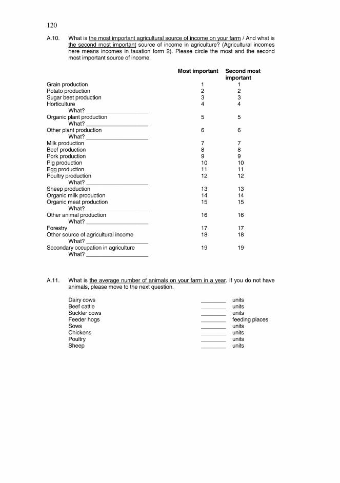
120

A.10. What is the most important agricultural source of income on your farm / And what isthe second most important source of income in agriculture? (Agricultural incomeshere means incomes in taxation form 2). Please circle the most and the secondmost important source of income.

Most important Second mostimportant

Grain production 1 1Potato production 2 2Sugar beet production 3 3Horticulture 4 4

What? ____________________Organic plant production 5 5

What? ____________________Other plant production 6 6

What? ____________________Milk production 7 7Beef production 8 8Pork production 9 9Pig production 10 10Egg production 11 11Poultry production 12 12

What? ____________________Sheep production 13 13Organic milk production 14 14Organic meat production 15 15

What? ____________________Other animal production 16 16

What? ____________________Forestry 17 17Other source of agricultural income 18 18

What? ____________________Secondary occupation in agriculture 19 19

What? ____________________

A.11. What is the average number of animals on your farm in a year. If you do not haveanimals, please move to the next question.

Dairy cows ________ unitsBeef cattle ________ unitsSuckler cows ________ unitsFeeder hogs ________ feeding placesSows ________ unitsChickens ________ unitsPoultry ________ unitsSheep ________ units

121

A.12. How much is the share of off-farm incomes of all incomes of your family? 1 No significant off-farm incomes

2 Under 25% of all incomes3 25-50% of all incomes

4 Over 50% of all incomes

A.13. Off-farm incomes consist mainly of (Please circle the most and the second mostimportant source of income)

Most important Second most important

Earned income 1 1Professional income (Taxation form 5) 2 2Business gain (Taxation form 6) 3 3Income from capital 4 4No off-farm incomes 5 5

A.14. Who in your family have off-farm incomes? 1 Mainly spouse 2 Mainly primary entrepreneur 3 Both 4 No off-farm incomes

A.15. Does your family have the possibility to get more off-farm incomes?1 No, because off-farm incomes are not available2 No, because current work contribution is required for the farm3 Yes

4 Unable to say

A.16. In what type of area is your farm located? 1 In an urban area 2 In a rural area 3 Near a populated area (less than 5 kilometre to the populated area) 4 In a sparsely populated area (over 5 kilometre to the populated area)

A.17. What is the family status? 1 Single

2 Married, no children3 Married, children

A.18. Do your children participate in agricultural work on your farm? 1 Regularly 2 Occasionally (during vocations etc.) 3 Do not participate 4 No children

A.19. Do you have hired staff on your farm (outside family)? 1 No 2 Yes, not more than one man year in a year 3 Yes, over one man year in a year

PLEASE TURN OVER

122

A.20. How many years ago did the shift from the previous generation on your farm takeplace? _____Years

A.21. When is the probable timing of the hand over to the next generation on your farm ? 1 After 0-5 years 2 After 5-15 years 3 After 15-25 years 4 Over 25 years 5 Farm quits production

A.22. Do you have a successor for the farm? 1 Yes 2 Uncertain 3 Not known

B.1. How often do you utilise a computer on the farm? 1 Regularly (at least once a week) 2 Once a week – once a month 3 Occasionally during the year 4 I don’t use a computer on the farm

B.2. How do you manage your bookkeeping for taxation? 1 Myself / with the family by computer 2 Myself / with the family by hand 3 Outside service used (accounting office etc.)

B.3. Did you make a budget for 1993? 1 Yes 2 No

B.4. How much is your family debt? _________FIM

B.5. How much were your agricultural incomes in 1992 (taxation form 2, entries 1-8)? _________FIM

B.6. How much was the clear profit from forestry in 1992 (taxation form 2A, entry 5)? _________FIM

B.7. How much are the expenditures of your private household a year?

_________FIM

B.8. How much is the average interest on your debt? 1 under 6 per cent 2 6-9 per cent 3 9-12 per cent 4 over 12 per cent

B.9. How big are your short term (term of loan is less than one year) debts of all debts? 1 under 25 percent 2 25-50 percent 3 over 50 percent

123

B.10. How much time do you spend on planning and control of production and economyduring wintertime?

1 0-2 hours a week 2 2-5 hours a week 3 5-10 hours a week 4 11-20 hours a week 5 over 20 hours a week

B.11. Have you written down (on paper) the objectives of your farm and family? 1 Yes 2 No

B.12. Does your farm have cooperation with other farms at the moment? 1 Not significantly 2 No cooperation, but jointly owned property 3 Yes, cooperation and jointly owned property

B.13. Which are the two most important sources for you to obtain information on agricul-ture (Please circle the most and the second most important source of information).

Most Second mostimportant important

Professional literature 1 1Advisory organisations and clubs 2 2Agricultural newspapers and magazines 3 3Radio / television 4 4Neighbours, friends 5 5Agricultural salesman 6 6Other, what? ______________________ 7 7

B.14. If Finland joins the European Community (EU), then agriculture faces considerablymore threats than possibilities. What is your opinion on this?(Answer using scale 1 to 5 so that 1=Fully agree and 5=Fully disagree).

Fully agree 1 2 3 4 5 Fully disagree

B.15. Society regulates agriculture by several means. Do you think that the regulation ofsociety in agriculture should be altered?

Regulation should be 1 2 3 4 5 Regulation should beincreased considerably decreased considerably

B.16. It has been proposed that the quota system in agriculture be changed so thatquotas are transferred from one farm to another using compensation, thus offeringthe possibility to purchase and sell quotas freely. What is your opinion on the pro-posal?

Fully agree 1 2 3 4 5 Fully disagree

PLEASE TURN OVER

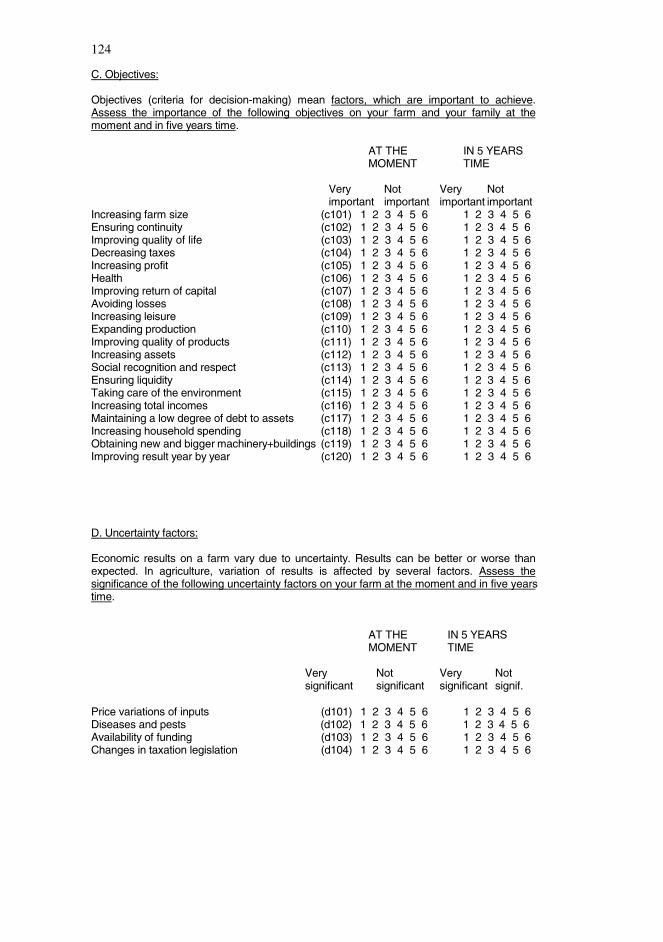
124

C. Objectives:

Objectives (criteria for decision-making) mean factors, which are important to achieve.Assess the importance of the following objectives on your farm and your family at themoment and in five years time.

AT THE IN 5 YEARSMOMENT TIME

Very Not Very Notimportant important important important

Increasing farm size (c101) 1 2 3 4 5 6 1 2 3 4 5 6Ensuring continuity (c102) 1 2 3 4 5 6 1 2 3 4 5 6Improving quality of life (c103) 1 2 3 4 5 6 1 2 3 4 5 6Decreasing taxes (c104) 1 2 3 4 5 6 1 2 3 4 5 6Increasing profit (c105) 1 2 3 4 5 6 1 2 3 4 5 6Health (c106) 1 2 3 4 5 6 1 2 3 4 5 6Improving return of capital (c107) 1 2 3 4 5 6 1 2 3 4 5 6Avoiding losses (c108) 1 2 3 4 5 6 1 2 3 4 5 6Increasing leisure (c109) 1 2 3 4 5 6 1 2 3 4 5 6Expanding production (c110) 1 2 3 4 5 6 1 2 3 4 5 6Improving quality of products (c111) 1 2 3 4 5 6 1 2 3 4 5 6Increasing assets (c112) 1 2 3 4 5 6 1 2 3 4 5 6Social recognition and respect (c113) 1 2 3 4 5 6 1 2 3 4 5 6Ensuring liquidity (c114) 1 2 3 4 5 6 1 2 3 4 5 6Taking care of the environment (c115) 1 2 3 4 5 6 1 2 3 4 5 6Increasing total incomes (c116) 1 2 3 4 5 6 1 2 3 4 5 6Maintaining a low degree of debt to assets (c117) 1 2 3 4 5 6 1 2 3 4 5 6Increasing household spending (c118) 1 2 3 4 5 6 1 2 3 4 5 6Obtaining new and bigger machinery+buildings (c119) 1 2 3 4 5 6 1 2 3 4 5 6Improving result year by year (c120) 1 2 3 4 5 6 1 2 3 4 5 6

D. Uncertainty factors:

Economic results on a farm vary due to uncertainty. Results can be better or worse thanexpected. In agriculture, variation of results is affected by several factors. Assess thesignificance of the following uncertainty factors on your farm at the moment and in five yearstime.

AT THE IN 5 YEARSMOMENT TIME

Very Not Very Notsignificant significant significant signif.

Price variations of inputs (d101) 1 2 3 4 5 6 1 2 3 4 5 6Diseases and pests (d102) 1 2 3 4 5 6 1 2 3 4 5 6Availability of funding (d103) 1 2 3 4 5 6 1 2 3 4 5 6Changes in taxation legislation (d104) 1 2 3 4 5 6 1 2 3 4 5 6

125

AT THE IN 5 YEARSMOMENT TIME

Very Not Very Notsignificant significant significant signif.

Fire, theft (d105) 1 2 3 4 5 6 1 2 3 4 5 6Adequacy of funding in the long term (d106) 1 2 3 4 5 6 1 2 3 4 5 6Outlet of products (d107) 1 2 3 4 5 6 1 2 3 4 5 6Fluctuation of interest (d108) 1 2 3 4 5 6 1 2 3 4 5 6Cultivation assurance of varieties (d109) 1 2 3 4 5 6 1 2 3 4 5 6Technological development (d110) 1 2 3 4 5 6 1 2 3 4 5 6Changes in world policy (d111) 1 2 3 4 5 6 1 2 3 4 5 6Adequacy of business skills (d112) 1 2 3 4 5 6 1 2 3 4 5 6Adequacy of securities (d113) 1 2 3 4 5 6 1 2 3 4 5 6Gap between planned and actual prices (d114) 1 2 3 4 5 6 1 2 3 4 5 6Variability of animal material quality (d115) 1 2 3 4 5 6 1 2 3 4 5 6Availability of additional incomes (d116) 1 2 3 4 5 6 1 2 3 4 5 6Availability of outside staff (d117) 1 2 3 4 5 6 1 2 3 4 5 6High level of inflation (d118) 1 2 3 4 5 6 1 2 3 4 5 6Existing investments (d119) 1 2 3 4 5 6 1 2 3 4 5 6Successor (d120) 1 2 3 4 5 6 1 2 3 4 5 6Degree of debt to own capital (d121) 1 2 3 4 5 6 1 2 3 4 5 6Joining the European Union (EU) (d122) 1 2 3 4 5 6 1 2 3 4 5 6Adequacy of education and professional skill (d123) 1 2 3 4 5 6 1 2 3 4 5 6Necessity to make short term investment (d124) 1 2 3 4 5 6 1 2 3 4 5 6Conflict between family and farm objectives (d125) 1 2 3 4 5 6 1 2 3 4 5 6Price variations of outputs (d126) 1 2 3 4 5 6 1 2 3 4 5 6Animals becoming ill (d127) 1 2 3 4 5 6 1 2 3 4 5 6Weak national economy (d128) 1 2 3 4 5 6 1 2 3 4 5 6Low level of inflation (d129) 1 2 3 4 5 6 1 2 3 4 5 6Changes in agricultural policy (d130) 1 2 3 4 5 6 1 2 3 4 5 6Funding in the short term (d131) 1 2 3 4 5 6 1 2 3 4 5 6Injuries (d132) 1 2 3 4 5 6 1 2 3 4 5 6Production quotas (d133) 1 2 3 4 5 6 1 2 3 4 5 6Price level between inputs and outputs (d134) 1 2 3 4 5 6 1 2 3 4 5 6Measures to limit production (d135) 1 2 3 4 5 6 1 2 3 4 5 6Availability and quality of information (d136) 1 2 3 4 5 6 1 2 3 4 5 6Costs (d137) 1 2 3 4 5 6 1 2 3 4 5 6Weather variations (d138) 1 2 3 4 5 6 1 2 3 4 5 6Conflict between the objectives of family (d139) 1 2 3 4 5 6 1 2 3 4 5 6Health (d140) 1 2 3 4 5 6 1 2 3 4 5 6Increasing requirement to market (d141) 1 2 3 4 5 6 1 2 3 4 5 6High level of household spending (d142) 1 2 3 4 5 6 1 2 3 4 5 6Changes in environmental legislation (d143) 1 2 3 4 5 6 1 2 3 4 5 6Information technology skills and knowledge (d144) 1 2 3 4 5 6 1 2 3 4 5 6Management of quality of products (d145) 1 2 3 4 5 6 1 2 3 4 5 6Costs of debt (d146) 1 2 3 4 5 6 1 2 3 4 5 6

PLEASE TURN OVER

126

D.2. What are the factors causing changes of the significance of uncertainty factors?

______________________________________________________________________________________________________________________________________________________________________________________________________

E. Risk management methods:

Uncertainty can be managed and reduced in several ways. Assess the importance of thefollowing methods to manage and reduce uncertainty on your farm.

Very NotImportant important

Cooperation between farms (e1) 1 2 3 4 5 6Low level of debt to assets (e2) 1 2 3 4 5 6Contract production (e3) 1 2 3 4 5 6Diversification (e4) 1 2 3 4 5 6Planning of investments (e5) 1 2 3 4 5 6Exercising stable production (e6) 1 2 3 4 5 6Insurance (e7) 1 2 3 4 5 6Part-time farming (e8) 1 2 3 4 5 6Planning and control of production (e9) 1 2 3 4 5 6Planning and control of marketing of products (e10) 1 2 3 4 5 6Acquisition of information (e11) 1 2 3 4 5 6Introducing additional processing of products on farm (e12) 1 2 3 4 5 6Unused credit reserves (e13) 1 2 3 4 5 6Exercising flexible production (e14) 1 2 3 4 5 6Increasing education and knowledge (e15) 1 2 3 4 5 6Low level of debt to turnover (e16) 1 2 3 4 5 6Dividing sales into periods (e17) 1 2 3 4 5 6Planning and control of economy (e18) 1 2 3 4 5 6Maintaining savings (e19) 1 2 3 4 5 6Maintaining liquidity (e20) 1 2 3 4 5 6Low level of short term loan to all loans (e21) 1 2 3 4 5 6Acquiring additional incomes (e22) 1 2 3 4 5 6

F. Expectations:

F.1. How do you estimate the price of your main product (see question A.10) to developin a year?

1 Price is over 10 per cent higher than the current price in a year 2 Price is 0-10 per cent higher than the current price in a year 3 Price is 0-5 per cent lower than the current price in a year 4 Price is over 5 than less than 10 per cent lower than the current price in a year 5 Price is 10-20 per cent lower than the current price in a year 6 Price is over 20 per cent lower than the current price in a year

127

F.2. Please explain your answer to the preceding price estimation.

______________________________________________________________________________________________________________________________________________________________________________________________________

G. Decision problems:

G.1. In agriculture, several decisions concerning farm economy and production aremade. The decision can be very significant or less significant. Assess the impor-tance of the following decisions for your farm.

Very Not significant significant

Planning of investments (g101) 1 2 3 4 5 6Planning of yearly production (g102) 1 2 3 4 5 6Budgeting (g103) 1 2 3 4 5 6Selection of plants and varieties (g104) 1 2 3 4 5 6Planning of work and leisure time (g105) 1 2 3 4 5 6Planning of liquidity (g106) 1 2 3 4 5 6Planning of taxation (g107) 1 2 3 4 5 6Planning of plant rotation (g108) 1 2 3 4 5 6Planning of marketing (g109) 1 2 3 4 5 6Planning of feeding (g110) 1 2 3 4 5 6Assessment of profitability (g111) 1 2 3 4 5 6Long term planning (g112) 1 2 3 4 5 6Planning of fertilisation (g113) 1 2 3 4 5 6Planning of plant protection (g114) 1 2 3 4 5 6

G.2. Which decision problems do you assess to be the most likely to require outside help(advises). Please mark the three most important matters.

Most Second most Third most Important important important

Planning of investments 1 2 3Planning of yearly production 1 2 3Budgeting 1 2 3Selection of plants and varieties 1 2 3Planning of work and leisure time 1 2 3Planning of liquidity 1 2 3Planning of taxation 1 2 3Planning of plant rotation 1 2 3Planning of marketing 1 2 3Planning of feeding 1 2 3Assessment of profitability 1 2 3Long term planning 1 2 3Planning of fertilisation 1 2 3Planning of plant protection 1 2 3

PLEASE TURN OVER

128

G.3. Many kinds of planning and control methods may be used in farm management.Some of these are listed below. Please assess the significance of each method foryour farm by circling the most suitable alternative.

Used Used Method known Method notregularly occasionally but not used known

Cross-margin method 1 2 3 4Linear optimisation 1 2 3 4Budgeting 1 2 3 4Production cost calculation 1 2 3 4

H. Values:

Characteristics associated with farming are presented in the following. How they reflect yourvalues in farming?

Very Notimportant important

Healthy lifestyle (h1) 1 2 3 4 5 6Possibility to gain profit (h2) 1 2 3 4 5 6Outdoor life (h3) 1 2 3 4 5 6Independence of work (h4) 1 2 3 4 5 6Respect received from work (h5) 1 2 3 4 5 6Possibility to work from home with the family (h6) 1 2 3 4 5 6Creativeness of work (h7) 1 2 3 4 5 6Entrepreneurship (h8) 1 2 3 4 5 6Possibility to develop oneself (h9) 1 2 3 4 5 6Possibility to take risks (h10) 1 2 3 4 5 6Belonging to a farm community (h11) 1 2 3 4 5 6Environmentally friendly production (h12) 1 2 3 4 5 6Job assurance (h13) 1 2 3 4 5 6Challenge in work (h14) 1 2 3 4 5 6Continuing family farm (h15) 1 2 3 4 5 6Possibility to express oneself (h16) 1 2 3 4 5 6Possibility to expand production (h17) 1 2 3 4 5 6Safety in work (h18) 1 2 3 4 5 6Possibility to earn reasonable incomes (h19) 1 2 3 4 5 6Possibility to do work one likes (h20) 1 2 3 4 5 6Entrepreneurship without risk (h21) 1 2 3 4 5 6Responsibility for work (h22) 1 2 3 4 5 6Possibility to work as one chooses (h23) 1 2 3 4 5 6

129

I. Attitudes toward risk:

The following presents examples of questions aimed at testing respondents attitudes towardrisk. Please circle the alternative which is the most agreeable to you. (Note that there is no‘right’ answer to the questions).

I.1. You are selling barley. You may sell barley immediately, when the price is fixed atFIM 1,80/kilogram or alternatively sell barley after three months, when there is a50% chance that the price will be FIM 2,00/kilogram or FIM 1,70/kilogram. Whichone would you choose?1 Sell immediately2 Sell after three months

I.2. You are filling in your taxation form. The tax in 1992 will be FIM 100 000. You may,however, make an investment for accounts, which may not be deductible. Thechance that it will be deductible is 50%, and then the amount of tax will be FIM 60000. If the investment is not deductible (50% chance), the amount of tax will in-crease to FIM 120 000. Which alternative would you choose?1 Not to make an investment2 Make an investment

I.3. Would you pay FIM 50 for a lottery ticket, where you win FIM 100 for only everyother ticket (50%) and nothing for the other ticket?1 Yes2 No

I.4. How much would you be willing to pay for the lottery ticket above? _______ FIM

I.5. How much would you be willing to pay for a lottery ticket, _______ FIMwhere you win FIM 100 with three out of four (75%) ticketsand nothing for the fourth (25%)?

I.6. How much would you be willing to pay for a lottery ticket, _______ FIMwhere you win FIM 100 with one out of four (25%) ticketsand nothing for three out of four (75%)?

I.7. You are given FIM 1000. You have to either take FIM 500 or a lottery ticket, whereyou win FIM 1000 for only every other ticket (50%) and nothing for the other ticket.Which one would you choose?1 FIM 5002 A lottery ticket

I.8. You are given FIM 2000. You have to either pay taxes of FIM 500 or take a lotteryticket, where every other ticket (50%) means FIM 1000 taxes and the other (50%)ticket releases you from paying taxes (taxes FIM 0). Which one would you choose?1 Pay FIM 5002 A lottery ticket

PLEASE TURN OVER

130

I.9. You are choosing plants for the next growing season. You can choose from threeplants and the yield is merely dependent on the forthcoming weather. The weatheris not known beforehand: it can be good, average or bad. The yield of plants A,Band C varies depending on the weather in the following way:

Yield of plant A varies: 300 (good weather), 200 (average weather), 100 (badweather).Yield of plant B varies: 600 (good weather), 200 (average weather), -200 (badweather).Yield of plant C varies: 400 (good weather), 300 (average weather), 0 (badweather).

Which plant would you choose based on information above?1 Plant A2 Plant B3 Plant C

I.10. Please explain your choice to the preceding question.

______________________________________________________________________________________________________________________________________________________________________________________________________

I.11. Which plant would you choose if you receive additional information on previousweather data: it can be expected that in two cases out of ten (20%) there will begood weather, four cases out of ten average weather (40%), and four cases out often (40%) a bad weather?1 Plant A2 Plant B3 Plant C

I.12. Would you be willing to pay for weather forecast mentioned above?1 Yes2 No

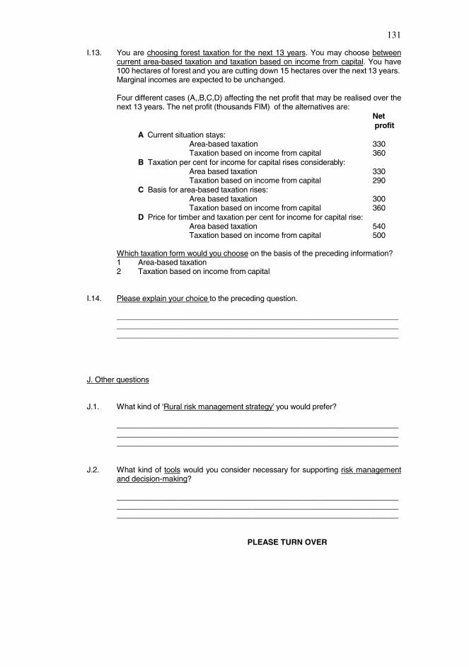
131

I.13. You are choosing forest taxation for the next 13 years. You may choose betweencurrent area-based taxation and taxation based on income from capital. You have100 hectares of forest and you are cutting down 15 hectares over the next 13 years.Marginal incomes are expected to be unchanged.

Four different cases (A,,B,C,D) affecting the net profit that may be realised over thenext 13 years. The net profit (thousands FIM) of the alternatives are:

Net profit

A Current situation stays: Area-based taxation 330Taxation based on income from capital 360

B Taxation per cent for income for capital rises considerably:Area based taxation 330Taxation based on income from capital 290

C Basis for area-based taxation rises:Area based taxation 300Taxation based on income from capital 360

D Price for timber and taxation per cent for income for capital rise:Area based taxation 540Taxation based on income from capital 500

Which taxation form would you choose on the basis of the preceding information?1 Area-based taxation2 Taxation based on income from capital

I.14. Please explain your choice to the preceding question.

______________________________________________________________________________________________________________________________________________________________________________________________________

J. Other questions

J.1. What kind of ‘Rural risk management strategy’ you would prefer?

______________________________________________________________________________________________________________________________________________________________________________________________________

J.2. What kind of tools would you consider necessary for supporting risk managementand decision-making?

______________________________________________________________________________________________________________________________________________________________________________________________________

PLEASE TURN OVER

132

J.3. What kind of investments do you plan to make during the next five years?

______________________________________________________________________________________________________________________________________________________________________________________________________

J.4. Should your farm be considered more as a separate entity or farm and farm familyas a unity when you assess the significance of risk on the farm? Please explainyour answer.

______________________________________________________________________________________________________________________________________________________________________________________________________

J.5. Please give your own comments on the subject.______________________________________________________________________________________________________________________________________________________________________________________________________

THANK YOU FOR YOUR ANSWERS !

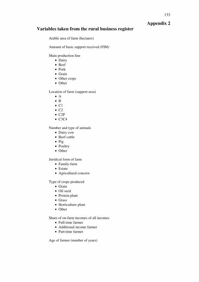
133

Appendix 2Variables taken from the rural business register

Arable area of farm (hectares)

Amount of basic support received (FIM)

Main production line• Dairy• Beef• Pork• Grain• Other crops• Other

Location of farm (support area)• A• B• C1• C2• C2P• C3C4

Number and type of animals• Dairy cow• Beef cattle• Pig• Poultry• Other

Juridical form of farm• Family-farm• Estate• Agricultural concern

Type of crops produced• Grain• Oil seed• Protein plant• Grass• Horticulture plant• Other

Share of on-farm incomes of all incomes• Full-time farmer• Additional income farmer• Part-time farmer

Age of farmer (number of years)

134

Appendix 3

STUDY OF FARMERS’ ADJUSTMENT INTO THE EU

Instructions: Please circle the alternative you consider to be correcton questions where alternatives are given.

A. Background questions

A.1. Year of birth? Year _______

A.2. How many years ago did the shift from the previous generation on your farm takeplace? ________Years

A.3. What is your basic education? 1 Elementary school 2 Basic school 3 Secondary school

A.4. What is your agricultural education? 1 No agricultural education 2 Courses etc. In agriculture 3 Agricultural school 4 Agricultural collage 5 Agricultural university

A.5. When is the probable timing of the hand over to the next generation on your farm ? 1 After 0-5 years 2 After 5-15 years 3 After 15-25 years 4 Over 25 years 5 Farm quits production

A.6. Do you have a successor for the farm? 1 Yes 2 Uncertain 3 Not known

A.7. How often do you utilise a computer on the farm? 1 Regularly (at least once a week) 2 Once a week – once a month 3 Occasionally during the year 4 I don’t use a computer on the farm

A.8. How you manage your bookkeeping for taxation? 1 Myself / with the family by computer 2 Myself / with the family by hand 3 Outside service used (accounting office etc.)

A.9. How much time do you spend on planning and control of production and economyduring wintertime?

1 0-2 hours a week 2 2-5 hours a week 3 over 5 hours a week

PLEASE TURN OVER

135

A.10. Have you made a budget 1998? 1 Yes 2 No

A.11. How much is your family debt?_________FIM

A.12. How much were your agricultural incomes in 1997 (taxation form 2, entry 21)?_________FIM

B. Farms’ adjustment into the EU:

B.1. Which of the following corresponds best to the solutions made on your farm during1993-1997? Choose the two most important items.

Most important Second mostimportant

(b11) (b12)Maintained current production 1 2Expanded production 1 2Reduced production 1 2Changed main production line 1 2Developed secondary occupation or additional processing 1 2Increased off-farm incomes 1 2Quit farming 1 2

B.2. What were the major reasons behind the preceding solutions?

___________________________________________________________________________________________________________________________________________________________________________________________________________________________

B.3. Was the decision based on economic plans, calculations and comparison ofalternatives?

1 Yes 2 No

B.4. What investments have you made during 1993-1997? Choose one or morealternatives.

1 Agricultural building 2 Tractor or combine harvester 3 Other machinery 4 Dung or liquid manure cistern 5 Subsurface drainage 6 Additional land 7 Other, what? _______________________________ 8 Nothing

B.5. What is your current position on the solutions proposed below for the farm duringthe next five years (1998-2002)? Choose the most obvious alternative.

1 Maintain current production 2 Expand production 3 Reduce production 4 Change main production line 5 Develop secondary occupation or additional processing

6 Increase off-farm incomes7 Quit production

8 Hand over to the next generation 9 Open solution, unable to answer

136

B.6. What investments do you plan to make during the next five years (1998-2002)?Choose one or more alternatives.

1 Agricultural building 2 Tractor or combine harvester 3 Other machinery 4 Dung or liquid manure cistern 5 Subsurface drainage 6 Additional land 7 Other, what? _______________________________ 8 Nothing

C. Objectives:

Objectives (criteria for decision-making) mean factors, which are important to achieve.Assess the importance of the following objectives on your farm and your family at themoment.

Very Not important important

Increasing farm size (c1) 1 2 3 4 5 6Ensuring continuity (c2) 1 2 3 4 5 6Improving quality of life (c3) 1 2 3 4 5 6Increasing profit (c4) 1 2 3 4 5 6Improving return of capital (c5) 1 2 3 4 5 6Avoiding losses (c6) 1 2 3 4 5 6Increasing leisure (c7) 1 2 3 4 5 6Expanding production (c8) 1 2 3 4 5 6Improving quality of products (c9) 1 2 3 4 5 6Increasing assets (c10) 1 2 3 4 5 6Ensuring liquidity (c11) 1 2 3 4 5 6Taking care of the environment (c12) 1 2 3 4 5 6Increasing total incomes (c13) 1 2 3 4 5 6Maintaining a low degree of debt to assets (c14) 1 2 3 4 5 6Increasing household spending (c15) 1 2 3 4 5 6Obtaining new and bigger machinery and buildings (c16) 1 2 3 4 5 6Reducing risk (c17) 1 2 3 4 5 6Increasing supports (c18) 1 2 3 4 5 6

D. Uncertainty factors:

Economic results on a farm vary due to uncertainty. Results can be better or worse thanexpected. In agriculture, variation of results is affected by several factors. Assess thesignificance of the following uncertainty factors on your farm at the moment.

Very Nosignificant significance

Availability and adequacy of funding (d1) 1 2 3 4 5 6Production risks in plant and animal production (d2) 1 2 3 4 5 6Accidents (d3) 1 2 3 4 5 6Outlet of products (d4) 1 2 3 4 5 6Adequacy of own knowledge, skills and education (d5) 1 2 3 4 5 6Changes in agricultural policy (d6) 1 2 3 4 5 6Variations in product price (d7) 1 2 3 4 5 6Maintaining liquidity (d8) 1 2 3 4 5 6Development and introduction of new technology (d9) 1 2 3 4 5 6

PLEASE TURN OVER

137

E. Risk management methods:

Uncertainty can be managed and reduced in several ways. Assess the importance of thefollowing methods to manage and reduce uncertainty on your farm.

Very NotImportant important

Planning and controlling production and economy (e1) 1 2 3 4 5 6Obtaining off-farm incomes (e2) 1 2 3 4 5 6Contract production (e3) 1 2 3 4 5 6Maintaining adequate liquidity and solvency (e4) 1 2 3 4 5 6Diversification (e5) 1 2 3 4 5 6

F. Values:

Characteristics associated with farming are presented as follows. How they reflect yourvalues in farming?

Very Notimportant important

Lifestyle (f1(2)) 1 2 3 4 5 6Possibility to gain profit (f2) 1 2 3 4 5 6Outdoor life (f3) 1 2 3 4 5 6Independence of work (f4) 1 2 3 4 5 6Respect received from work (f5) 1 2 3 4 5 6Entrepreneurship (f6) 1 2 3 4 5 6Possibility to develop oneself (f7) 1 2 3 4 5 6Belonging to a farm community (f8) 1 2 3 4 5 6Environmentally friendly production (f9) 1 2 3 4 5 6Job assurance (f10) 1 2 3 4 5 6Challenge in work (f11) 1 2 3 4 5 6Continuing family farm (f12) 1 2 3 4 5 6Possibility to express oneself (f13) 1 2 3 4 5 6Possibility to expand production (f14) 1 2 3 4 5 6Possibility to earn reasonable incomes (f15) 1 2 3 4 5 6Possibility to work as one chooses (f16) 1 2 3 4 5 6Versatility of work (f17) 1 2 3 4 5 6

G. Attitudes toward risk:

The following presents examples of questions aimed at testing respondents attitudes towardrisk. Please circle the alternative which is the most agreeable to you. (Note that there is no‘right’ answer to the questions).

G.1. Would you pay FIM 50 for a lottery ticket, where you win FIM 100 for only everyother ticket (50%) and nothing for the other ticket?1 Yes2 No

G.2. How much would you be willing to pay for the lottery ticket above? ________ FIM

THANK YOU FOR YOUR ANSWERS!

138

Appendix 4

16.2.1998

STUDY OF FARMERS’ ADJUSTMENT INTO THEEU

Dear recipient

You were involved in the study of risk and decision-making being carried out bythe Association of Rural Advisory Centres in spring 1993. The study was con-ducted by Sauli Sonkkila. Your participation in the study was very valuable. Theresults of the study indicated which issues farmers considered important andwhere decision-makers should pay attention when making decisions concerningagriculture.

The operational environment of farms has been changing greatly during mem-bership of the EU, so the questions asked in 1993 may have altered a lot duringthe five year period of study. Therefore, it is important to carry out a limited fol-low-up survey. The purpose of this study is to find out, what kind of solutionsfarms have reached during the membership of EU and what factors influencedthese decisions.

This inquiry has been sent to different parts of Finland to all those 500 farmswhich responded to the 1993 survey.

We appreciate that filling in the questionnaire demands your time and energy.We are very grateful for your understanding contribution to this study. We hopethat the results will lead to a better understanding of the current situation farmsface and therefore assist farms to manage well in the future.

We ask you to return the form using the enclosed envelope by 2 March 1998 atthe latest. You may also send this form by telefax (09-13421496).

The information received is fully confidential and will be used only for this study.The data are processed statistically and no single respondents data or opinionswill be revealed.

This study is carried out by Sauli Sonkkila with the support of the Finnish Cul-tural Foundation, the Information Centre of the Ministry of Agriculture and For-estry and the University of Helsinki. Mr Sonkkila will provide any additional in-formation on questions relating this study (tel. 09-13421234).

YOURS FAITHFULLY

Sauli Sonkkila Niilo Hintikka Matti YlätaloResearcher Director General Professor, Agric. Econ.MMM/TIKE MMM/TIKE University of Helsinki

139

Appendix 5

Principal component analysis for objective variables

LATENT ROOTS (EIGENVALUES)

1 2 3 4 5

4.425 2.037 1.497 1.339 1.070

6 7 8 9 10

0.948 0.905 0.821 0.723 0.658

11 12 13 14 15

0.571 0.558 0.540 0.492 0.412

16 17 18

0.393 0.327 0.285

ROTATED LOADINGS

C2PCA1 C2PCA2 C2PCA3 C2PCA4 C2PCA5

C1 0.810 0.004 0.162 -0.092 0.073 C2 0.529 0.211 0.271 -0.118 0.277 C3 -0.090 0.172 0.312 0.570 0.315 C4 0.159 0.136 0.818 0.152 -0.043 C5 0.148 0.233 0.756 -0.018 0.019 C6 0.124 0.650 0.132 0.076 0.070 C7 -0.197 0.120 -0.033 0.666 0.205 C8 0.806 0.030 0.221 -0.038 0.137 C9 0.391 0.001 0.105 0.201 0.586 C10 0.401 -0.030 0.508 0.392 -0.084 C11 0.020 0.482 0.176 -0.048 0.555 C12 0.018 0.044 -0.006 0.047 0.749 C13 0.173 0.032 0.774 0.141 0.107 C14 0.008 0.677 0.039 0.155 -0.112 C15 0.292 0.072 0.017 0.692 -0.184 C16 0.759 0.034 0.023 0.178 -0.081 C17 -0.011 0.693 0.100 0.030 0.213 C18 0.038 0.042 0.551 -0.086 0.119

VARIANCE EXPLAINED BY ROTATED COMPONENTS

C2PCA1 C2PCA2 C2PCA3 C2PCA4 C2PCA5

2.703 1.767 2.721 1.583 1.594

PERCENT OF TOTAL VARIANCE EXPLAINED

C2PCA1 C2PCA2 C2PCA3 C2PCA4 C2PCA5

15.018 9.819 15.118 8.793 8.854

140

Appendix 6

Principal component analysis for value variables

LATENT ROOTS (EIGENVALUES)

1 2 3 4 5

6.577 1.397 1.017 0.926 0.890

6 7 8 9 10

0.836 0.684 0.645 0.635 0.564

11 12 13 14 15

0.531 0.507 0.438 0.384 0.367

16 17

0.317 0.286

ROTATED LOADINGS

F2PCA1 F2PCA2 F2PCA3 F2PCA4

F1(2) 0.095 0.768 -0.052 0.186 F2 0.656 -0.178 0.196 0.160 F3 -0.004 0.584 0.189 0.422 F4 0.113 0.081 0.116 0.740 F5 0.509 0.136 0.498 0.244 F6 0.365 -0.037 0.436 0.506 F7 0.160 0.010 0.520 0.552 F8 0.048 0.268 0.722 0.181 F9 0.073 0.560 0.499 -0.012 F10 0.643 0.305 0.251 0.156 F11 0.383 0.270 0.300 0.454 F12 0.487 0.330 0.332 0.108 F13 0.297 0.165 0.415 0.544 F14 0.331 -0.102 0.601 0.222 F15 0.789 0.078 -0.059 0.278 F16 0.365 0.298 0.171 0.596 F17 0.238 0.305 0.070 0.705

VARIANCE EXPLAINED BY ROTATED COMPONENTS

F2PCA1 F2PCA2 F2PCA3 F2PCA4

2.685 1.874 2.404 2.954

PERCENT OF TOTAL VARIANCE EXPLAINED

F2PCA1 F2PCA2 F2PCA3 F2PCA4

15.792 11.022 14.142 17.377

141

Appendix 7

Correlation between continuos variables

A1(1) A8(1) A101 A111 A20 B4 B5(1) C101 C102

A1(1) 1.000 A8(1) 0.175 1.000 A101 -0.213 -0.036 1.000 A111 0.017 0.626 0.118 1.000 A20 0.605 0.182 -0.152 0.050 1.000 B4 -0.178 0.244 0.062 0.257 -0.264 1.000 B5(1) 0.113 0.663 0.045 0.662 0.062 0.518 1.000 C101 0.188 -0.091 0.207 -0.047 0.341 -0.156 -0.064 1.000 C102 0.187 -0.000 -0.079 -0.096 0.231 -0.265 -0.173 0.243 1.000 C103 0.106 -0.020 0.066 0.141 0.093 0.058 0.096 0.041 0.141 C104 0.230 -0.071 0.128 -0.066 0.216 -0.105 -0.152 0.191 0.185 C105 -0.106 -0.114 -0.012 -0.057 -0.092 0.070 -0.176 -0.065 -0.032 C106 0.034 -0.021 -0.022 -0.107 0.048 0.106 -0.043 0.048 0.193 C107 -0.022 -0.059 -0.012 -0.056 0.006 -0.051 -0.139 0.058 0.020 C108 -0.162 -0.182 0.453 0.026 -0.308 -0.006 -0.225 -0.052 -0.037 C109 0.004 0.131 0.252 0.101 0.043 0.133 0.087 0.282 0.075 C110 0.068 0.089 -0.009 -0.121 0.108 -0.078 -0.122 0.397 0.311 C111 0.096 -0.061 -0.070 0.195 -0.015 -0.024 -0.112 -0.040 0.160 C112 0.051 0.107 0.058 -0.018 0.094 -0.075 -0.055 0.174 0.330 C113 0.174 0.118 -0.114 0.094 0.203 -0.094 0.033 0.110 0.164 C114 0.098 -0.048 -0.052 0.063 0.053 -0.278 -0.179 0.043 0.234 C115 -0.136 0.002 0.176 0.109 -0.043 -0.037 0.057 0.055 0.154 C116 0.028 -0.012 -0.063 0.029 0.035 -0.045 -0.201 0.098 0.048 C117 0.129 -0.005 -0.116 0.047 0.015 -0.359 -0.142 -0.132 0.093 C118 0.209 0.049 -0.145 0.084 0.017 -0.088 0.017 0.146 0.336 C119 0.079 -0.031 -0.169 0.036 0.087 -0.172 -0.186 0.121 0.193 C120 -0.049 0.104 0.053 0.150 -0.053 0.153 -0.051 0.110 0.106 H1 0.346 -0.206 -0.087 -0.242 0.093 -0.279 -0.237 0.014 0.273 H2 0.036 -0.212 -0.035 -0.158 0.081 -0.260 -0.337 0.165 0.283 H3 -0.055 -0.058 -0.149 0.002 0.017 -0.106 0.094 -0.014 0.065 H4 0.074 -0.193 -0.073 -0.015 0.066 -0.167 -0.081 0.017 0.061 H5 0.207 -0.118 -0.139 -0.081 0.024 -0.261 -0.187 0.219 0.246 H6 0.344 0.023 -0.103 0.137 0.019 0.030 0.080 -0.035 0.040 H7 0.154 -0.112 -0.030 -0.092 -0.041 -0.085 -0.089 0.065 0.160 H8 0.244 0.021 0.008 0.075 -0.057 -0.018 -0.009 0.048 0.078 H9 0.067 0.030 -0.120 -0.006 0.178 -0.047 -0.150 0.063 0.222 H10 0.027 -0.036 -0.174 -0.105 -0.014 -0.113 -0.181 -0.062 0.037 H11 0.048 -0.113 -0.169 -0.107 0.141 -0.290 -0.158 0.108 0.335 H12 0.161 -0.142 -0.042 -0.062 -0.020 -0.170 -0.220 -0.011 0.144 H13 -0.042 -0.175 -0.103 0.036 -0.154 -0.120 -0.238 -0.115 0.227 H14 -0.177 -0.122 -0.111 0.085 -0.218 0.152 -0.068 -0.010 0.103 H15 0.256 -0.007 -0.089 0.038 0.156 -0.239 -0.120 0.194 0.427 H16 0.067 -0.165 -0.108 -0.123 0.110 -0.286 -0.214 0.124 0.188 H17 0.082 0.003 -0.157 -0.013 0.107 -0.147 -0.203 0.237 0.443 H18 0.134 -0.298 -0.140 -0.121 -0.054 -0.214 -0.375 0.028 0.183 H19 0.086 -0.276 0.005 0.029 -0.027 -0.052 -0.288 0.055 0.186 H20 -0.097 -0.142 0.047 0.018 -0.129 -0.003 -0.067 0.051 0.083 H21 0.097 -0.221 0.067 -0.190 -0.158 -0.175 -0.257 0.165 0.277 H22 -0.061 -0.126 0.000 0.022 -0.076 -0.146 -0.183 0.070 0.213 H23 -0.068 -0.008 -0.113 -0.016 -0.057 -0.131 0.007 -0.027 0.276 I4 -0.080 0.010 -0.265 0.008 -0.019 -0.092 -0.166 0.019 -0.049 A1(2) -0.706 -0.305 0.238 -0.199 -0.466 0.114 -0.229 -0.129 -0.098 A2(2) 0.502 0.181 -0.213 0.134 0.633 -0.101 0.122 0.199 0.113 A11 -0.210 0.327 0.076 0.274 -0.242 0.746 0.404 -0.116 -0.028 A12(2) -0.033 0.603 0.112 0.629 -0.136 0.461 0.701 -0.094 -0.005 C1 0.056 0.188 0.147 0.099 0.028 0.080 0.033 0.390 0.214 C2 0.258 0.186 -0.119 0.169 0.222 -0.100 -0.007 0.165 0.429 C3 -0.150 0.106 -0.117 0.132 -0.078 -0.001 0.015 -0.085 -0.185 C4 0.025 0.026 -0.060 -0.040 0.042 0.169 -0.134 0.115 0.093 C5 -0.034 0.005 -0.142 -0.012 0.033 0.167 -0.076 0.144 -0.030 C6 0.052 0.036 -0.051 0.051 -0.085 0.082 -0.041 -0.075 0.122 C7 -0.107 -0.045 0.342 0.055 0.022 -0.282 -0.232 0.053 0.167 C8 0.034 0.251 0.145 0.158 0.022 0.216 0.067 0.200 0.145 C9 0.091 0.236 0.226 0.260 0.076 0.086 0.051 0.285 0.072 C10 0.002 -0.020 0.173 -0.169 -0.015 -0.095 -0.285 0.157 0.158 C11 -0.068 0.061 -0.068 0.077 -0.179 0.172 0.060 -0.028 0.108 C12 0.171 0.012 -0.126 0.032 0.060 -0.044 -0.067 0.203 0.161 C13 0.056 -0.013 -0.137 -0.112 0.020 -0.018 -0.236 0.178 0.110 C14 0.004 -0.168 -0.095 -0.186 -0.069 0.004 -0.164 -0.015 -0.174 C15 0.071 0.181 -0.053 0.024 0.071 -0.011 0.036 -0.114 0.250 C16 0.091 0.180 -0.098 0.057 0.101 0.098 -0.006 0.147 -0.096 C17 0.021 0.001 0.006 -0.156 0.042 -0.032 -0.154 -0.071 0.010 C18 0.280 0.167 -0.126 0.040 0.262 -0.105 -0.103 0.126 0.142 D1 0.061 0.121 -0.141 -0.027 0.094 -0.005 -0.205 0.195 0.200 D2 0.229 0.084 -0.134 0.074 0.264 0.034 -0.001 -0.183 0.120 D3 0.112 -0.051 -0.121 -0.027 0.206 -0.153 -0.112 -0.132 0.254 D4 0.414 0.037 -0.107 -0.036 0.284 -0.069 0.025 0.192 0.243 D5 0.210 -0.044 0.119 0.095 0.070 0.079 -0.046 0.119 -0.149 D6 0.199 0.146 -0.078 0.229 0.110 -0.036 0.178 -0.069 0.057 D7 0.323 0.088 -0.088 0.162 0.239 -0.015 0.056 -0.064 0.295 D8 0.129 -0.101 -0.076 -0.050 0.090 -0.009 -0.035 0.044 0.034 D9 0.156 0.123 -0.195 0.052 0.050 0.070 -0.024 0.098 -0.078 E1 0.215 0.133 -0.079 0.216 -0.131 0.036 0.171 -0.058 0.108 E2 0.083 -0.053 0.205 -0.167 -0.010 -0.131 -0.263 -0.053 0.086 E3 0.145 0.170 -0.009 0.247 0.125 0.091 0.163 0.134 0.189 E4 0.162 0.001 -0.083 0.164 0.091 0.037 0.108 0.093 0.157 E5 0.218 -0.147 -0.221 -0.303 0.081 -0.063 -0.251 0.013 0.180 F1(2) 0.178 0.071 -0.125 -0.032 0.352 -0.121 0.010 0.107 0.243 F2 0.025 0.181 -0.058 0.117 0.128 0.011 -0.063 0.065 0.254 F3 -0.004 0.020 0.351 -0.114 0.010 -0.161 -0.056 -0.066 -0.016 F4 0.109 -0.109 -0.103 -0.084 0.080 -0.259 -0.181 0.030 0.148 F5 0.194 0.045 -0.158 0.055 -0.040 0.012 -0.140 -0.080 0.125 F6 0.037 0.105 -0.132 0.125 -0.113 -0.008 -0.077 0.010 0.067 F7 0.174 0.023 -0.167 -0.059 -0.028 -0.050 -0.109 -0.013 0.042 F8 0.289 0.051 -0.186 0.001 0.155 0.024 -0.054 0.004 0.197 F9 0.234 -0.111 -0.162 -0.106 0.229 -0.153 -0.182 0.100 0.238 F10 0.278 0.003 -0.104 0.115 0.216 -0.170 -0.062 -0.010 0.277 F11 0.211 0.166 0.176 0.217 0.129 -0.138 0.088 0.167 0.342 F12 0.336 0.167 -0.122 0.077 0.123 -0.218 -0.106 0.101 0.382 F13 0.167 0.052 -0.142 -0.003 0.009 -0.153 -0.054 0.111 0.263 F14 0.244 0.276 -0.169 0.168 0.109 0.093 0.064 0.152 0.108 F15 0.061 -0.032 -0.109 -0.000 0.008 -0.001 -0.026 -0.184 0.113 F16 0.205 0.032 -0.105 -0.115 0.013 -0.130 -0.102 0.004 0.163 F17 0.009 0.009 -0.120 -0.089 0.127 -0.016 -0.018 0.008 0.150 G2 -0.092 0.114 0.074 0.178 -0.036 0.016 0.068 0.089 -0.131 VILJELYA 0.051 0.778 -0.038 0.536 0.028 0.270 0.557 0.079 0.112 IKA97 0.706 0.305 -0.238 0.199 0.466 -0.114 0.229 0.129 0.098 C2PCA1 0.130 0.268 0.097 0.142 0.092 0.126 0.070 0.277 0.194 C2PCA2 -0.010 -0.091 -0.132 -0.139 -0.104 0.074 -0.092 -0.170 -0.051 C2PCA3 0.049 -0.011 -0.146 -0.085 0.071 0.044 -0.195 0.141 0.071 C2PCA4 -0.109 0.049 0.160 0.012 -0.019 -0.161 -0.134 -0.075 0.033 C2PCA5 0.081 0.185 0.075 0.295 0.025 0.001 0.081 0.228 0.184 LYPSYL97 -0.036 0.602 0.145 0.809 -0.011 0.277 0.559 0.056 -0.024 LIHAK97 -0.089 0.481 0.015 0.416 -0.107 0.197 0.403 -0.057 -0.050 FPCA1 0.167 0.140 -0.128 0.184 0.118 -0.043 -0.029 -0.030 0.318 FPCA2 0.213 -0.080 0.075 -0.138 0.315 -0.249 -0.066 0.037 0.251 FPCA3 0.267 0.120 -0.177 0.082 0.053 0.032 -0.064 0.105 0.124 FPCA4 -0.094 -0.039 0.033 -0.111 -0.113 -0.085 -0.034 -0.019 -0.051

142

C103 C104 C105 C106 C107 C108 C109 C110 C111

C103 1.000 C104 0.173 1.000 C105 0.252 0.473 1.000 C106 -0.019 0.207 0.137 1.000 C107 0.213 0.367 0.604 0.041 1.000 C108 0.072 0.224 0.353 -0.015 0.342 1.000 C109 0.337 0.203 0.229 0.047 0.118 0.118 1.000 C110 0.003 0.074 0.036 0.233 0.026 -0.111 0.242 1.000 C111 0.122 0.017 0.225 0.186 0.305 0.439 -0.042 0.012 1.000 C112 0.248 0.367 0.346 0.028 0.242 0.162 0.207 0.194 0.068 C113 0.106 0.133 0.132 0.236 0.166 0.060 0.296 0.075 0.299 C114 0.000 0.202 0.152 0.102 0.335 0.371 -0.046 0.086 0.522 C115 0.109 0.007 0.086 0.394 0.244 0.228 -0.006 -0.053 0.465 C116 0.216 0.474 0.682 0.183 0.542 0.298 0.248 0.140 0.271 C117 0.142 0.319 0.202 0.026 0.306 0.327 -0.070 -0.109 0.330 C118 0.099 0.180 0.074 0.094 0.102 -0.153 0.168 0.124 0.135 C119 0.238 0.146 0.169 0.097 0.118 0.004 0.358 0.292 0.263 C120 0.062 0.298 0.267 0.042 0.305 0.336 0.314 0.225 0.354 H1 -0.024 0.114 -0.074 0.335 -0.031 -0.006 -0.084 0.043 0.069 H2 0.047 0.248 0.400 -0.011 0.186 0.220 0.134 0.047 0.179 H3 0.084 0.101 0.049 0.104 -0.080 0.057 -0.106 -0.092 -0.004 H4 -0.038 0.069 0.117 0.067 0.011 0.136 -0.101 -0.101 0.212 H5 -0.141 0.025 -0.065 0.102 -0.069 0.057 0.055 -0.015 0.167 H6 0.148 0.045 -0.010 0.023 0.025 0.170 -0.025 -0.211 0.182 H7 -0.050 -0.020 -0.046 0.102 -0.075 0.024 -0.112 -0.045 0.073 H8 -0.065 -0.059 -0.077 0.117 -0.105 -0.001 -0.158 0.044 0.064 H9 -0.013 0.037 0.135 0.211 0.060 -0.082 0.033 0.154 0.201 H10 -0.071 -0.048 -0.019 0.262 -0.029 -0.215 -0.085 0.034 0.009 H11 0.011 0.121 -0.088 0.151 -0.008 -0.065 -0.002 0.174 0.142 H12 -0.067 0.098 -0.008 0.331 0.159 0.078 -0.096 0.016 0.368 H13 -0.161 0.104 -0.000 0.139 0.091 0.211 -0.135 0.039 0.257 H14 0.015 0.150 0.227 0.349 0.132 0.050 -0.043 0.210 0.241 H15 0.068 0.227 0.130 0.231 0.113 0.078 0.104 0.208 0.219 H16 0.092 0.200 0.112 0.153 0.187 0.087 -0.010 0.069 0.265 H17 0.004 0.312 0.189 0.317 0.166 -0.055 0.161 0.483 0.024 H18 0.010 0.333 0.105 0.246 0.126 0.116 -0.213 0.029 0.147 H19 0.114 0.301 0.182 0.211 0.142 0.217 0.033 0.088 0.260 H20 0.014 0.052 0.082 0.436 0.025 0.184 -0.112 -0.046 0.175 H21 0.007 0.248 -0.036 0.152 0.122 -0.048 0.050 0.162 -0.053 H22 -0.047 0.361 0.060 0.238 0.250 0.172 0.107 0.152 0.275 H23 -0.024 0.290 0.143 0.340 0.163 0.050 0.016 0.159 0.161 I4 -0.137 -0.084 0.066 0.058 -0.002 -0.159 -0.054 0.010 0.026 A1(2) -0.068 -0.070 0.250 -0.004 0.196 0.262 0.086 0.085 0.000 A2(2) 0.024 0.040 -0.286 0.028 -0.230 -0.407 -0.102 -0.091 -0.028 A11 0.022 -0.145 0.069 0.161 -0.021 0.081 0.059 0.128 0.115 A12(2) 0.027 -0.146 -0.016 -0.056 0.044 0.052 0.065 -0.045 0.148 C1 -0.011 0.089 -0.080 0.088 0.145 -0.011 0.160 0.337 -0.093 C2 -0.016 0.213 0.057 0.128 0.172 -0.042 0.052 0.145 0.138 C3 0.083 -0.177 0.045 -0.079 -0.081 0.013 0.144 0.005 0.050 C4 -0.066 0.085 0.254 0.043 0.167 0.236 0.286 0.188 0.232 C5 -0.010 -0.082 0.136 -0.067 0.174 0.121 0.243 0.207 0.210 C6 0.097 0.030 0.150 0.021 0.180 0.315 0.040 0.013 0.216 C7 -0.032 0.120 0.257 -0.096 0.098 0.429 0.220 -0.019 0.244 C8 -0.031 0.049 -0.036 0.136 0.144 0.053 0.071 0.447 0.001 C9 -0.008 0.211 0.123 0.129 0.200 0.230 0.227 0.264 0.283 C10 0.073 0.077 0.155 -0.046 0.170 0.136 0.343 0.237 0.067 C11 -0.002 0.078 0.070 0.377 0.102 0.088 0.096 0.149 0.091 C12 0.057 -0.011 -0.094 0.176 0.044 0.026 -0.072 0.116 0.275 C13 -0.119 0.059 0.116 0.244 0.080 0.098 0.279 0.318 0.188 C14 0.020 -0.116 0.045 -0.116 0.240 0.102 -0.030 -0.117 -0.031 C15 0.093 -0.105 0.089 -0.085 0.140 -0.068 0.061 0.149 0.228 C16 -0.124 0.113 0.149 0.084 0.373 0.031 0.032 0.223 0.260 C17 0.138 0.018 0.104 -0.019 0.074 0.118 0.099 -0.067 -0.053 C18 0.103 0.333 0.085 0.010 0.171 -0.006 0.235 0.107 0.026 D1 -0.205 0.190 0.173 0.244 0.150 0.061 0.101 0.406 0.241 D2 -0.003 0.121 0.029 0.081 -0.007 -0.097 -0.008 -0.121 -0.016 D3 0.147 -0.005 -0.021 0.326 -0.075 -0.072 0.149 0.042 0.115 D4 -0.032 0.229 -0.113 0.325 -0.060 -0.068 0.106 0.252 0.003 D5 -0.000 0.071 0.094 0.038 0.051 0.086 0.122 0.118 0.102 D6 0.094 0.101 -0.005 0.049 0.089 0.102 0.060 -0.151 -0.016 D7 0.126 0.062 0.035 0.224 0.008 -0.005 0.125 -0.030 0.107 D8 -0.031 0.124 0.038 0.562 -0.000 0.100 0.004 0.121 0.044 D9 -0.022 -0.183 -0.027 -0.018 0.051 -0.149 0.127 0.159 0.173 E1 -0.128 -0.186 -0.202 0.063 -0.207 -0.135 0.003 0.033 0.063 E2 0.016 0.074 0.119 0.174 0.019 0.174 0.138 -0.038 0.161 E3 -0.024 0.125 -0.152 0.182 -0.200 -0.155 0.072 0.219 0.046 E4 0.152 0.089 0.068 0.014 0.128 0.213 -0.088 -0.111 0.200 E5 0.009 0.039 0.131 0.265 0.079 -0.111 0.003 0.311 0.148 F1(2) 0.074 0.198 0.074 0.037 -0.054 -0.013 0.067 0.001 -0.031 F2 -0.039 0.316 0.321 0.205 0.127 0.193 0.291 0.159 0.260 F3 -0.125 0.268 0.159 0.329 -0.006 0.156 -0.026 -0.141 -0.146 F4 -0.237 0.133 0.067 0.395 0.024 0.099 -0.134 0.053 0.072 F5 -0.174 0.216 0.054 0.336 0.025 0.119 -0.056 -0.002 0.305 F6 -0.105 -0.019 0.075 0.266 -0.105 0.041 -0.008 0.123 0.183 F7 -0.209 -0.061 -0.175 0.014 -0.250 -0.107 -0.078 -0.007 -0.020 F8 -0.071 0.140 -0.031 0.112 -0.025 -0.045 -0.077 -0.024 -0.003 F9 0.055 0.145 -0.200 0.004 -0.022 -0.167 -0.058 0.039 0.020 F10 -0.076 0.226 -0.089 -0.090 -0.027 0.034 -0.159 -0.144 0.088 F11 0.008 0.150 -0.131 0.036 0.009 -0.054 -0.093 0.019 -0.068 F12 -0.033 0.240 0.089 0.195 0.093 0.016 -0.083 0.092 0.131 F13 -0.054 -0.065 -0.088 0.208 -0.100 -0.111 -0.041 0.070 0.064 F14 -0.183 0.118 -0.069 0.176 -0.045 -0.157 -0.084 0.273 -0.011 F15 -0.137 0.039 -0.006 0.291 -0.007 0.169 -0.097 -0.013 0.248 F16 -0.076 0.174 0.008 0.447 -0.105 -0.052 -0.170 0.110 -0.060 F17 -0.001 0.141 0.095 0.480 -0.137 -0.098 -0.108 0.023 -0.056 G2 -0.021 -0.012 -0.034 -0.161 -0.073 -0.145 0.054 -0.028 -0.244 VILJELYA 0.036 0.086 0.057 0.018 0.076 -0.154 0.128 0.282 -0.044 IKA97 0.068 0.070 -0.250 0.004 -0.196 -0.262 -0.086 -0.085 -0.000 C2PCA1 -0.046 0.117 -0.000 0.106 0.280 -0.015 0.055 0.377 0.084 C2PCA2 0.098 -0.079 0.109 -0.026 0.219 0.172 -0.046 -0.155 -0.010 C2PCA3 -0.025 0.090 0.159 0.056 0.067 0.102 0.351 0.216 0.126 C2PCA4 0.047 -0.103 0.203 -0.180 0.095 0.188 0.186 0.044 0.273 C2PCA5 0.017 0.188 -0.030 0.344 -0.025 0.113 0.088 0.191 0.217 LYPSYL97 0.188 -0.071 0.037 -0.108 0.058 -0.022 0.251 0.031 0.067 LIHAK97 0.062 -0.126 0.037 -0.127 0.026 -0.026 -0.052 0.070 0.023 FPCA1 -0.048 0.257 0.137 0.157 0.118 0.189 0.039 0.067 0.346 FPCA2 0.133 0.271 -0.033 0.019 0.015 -0.024 -0.089 -0.172 -0.136 FPCA3 -0.098 0.051 -0.136 -0.027 -0.045 -0.149 -0.043 0.103 0.025 FPCA4 -0.146 -0.063 0.048 0.418 -0.162 -0.007 -0.101 0.032 -0.104

C112 C113 C114 C115 C116 C117 C118 C119 C120

C112 1.000 C113 -0.059 1.000 C114 -0.037 0.249 1.000 C115 0.041 0.298 0.343 1.000 C116 0.499 0.261 0.181 0.148 1.000 C117 0.093 0.256 0.452 0.110 0.327 1.000 C118 0.362 0.011 -0.066 0.061 0.120 -0.159 1.000 C119 0.255 0.234 0.044 0.002 0.318 -0.012 0.374 1.000 C120 0.353 0.157 0.168 0.070 0.374 0.101 0.207 0.401 1.000 H1 -0.198 0.133 0.111 0.073 0.027 0.143 0.107 0.166 0.028 H2 0.305 0.201 0.136 -0.051 0.260 0.198 0.244 0.157 0.309 H3 -0.105 -0.070 0.138 0.038 -0.049 0.175 -0.119 -0.055 -0.101 H4 0.120 -0.012 0.302 0.110 0.113 0.221 0.142 -0.095 -0.064 H5 0.021 0.428 0.087 0.124 0.118 0.089 0.152 0.192 0.030 H6 -0.032 0.101 0.240 -0.012 0.084 0.167 0.060 -0.020 0.012

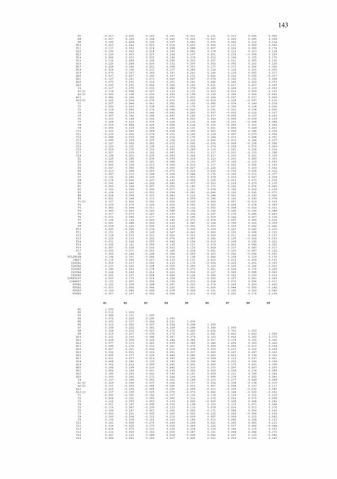
143 H7 -0.017 0.202 0.163 -0.101 -0.031 0.121 -0.013 0.045 -0.002 H8 -0.057 0.189 0.148 -0.043 -0.032 -0.027 0.025 0.065 0.008 H9 0.182 0.408 0.190 0.167 0.083 0.076 0.043 0.112 0.114 H10 -0.023 0.244 0.023 0.018 0.030 -0.006 0.131 0.050 -0.062 H11 0.137 0.293 0.218 0.268 0.088 -0.007 0.244 0.280 0.174 H12 -0.195 0.342 0.218 0.325 0.081 0.178 0.115 0.157 0.118 H13 -0.125 0.063 0.327 0.164 0.107 0.201 0.132 -0.008 0.169 H14 0.066 0.303 0.222 0.184 0.318 0.012 0.104 0.125 0.172 H15 0.116 0.489 0.346 0.284 0.343 0.207 0.221 0.365 0.145 H16 0.125 0.248 0.409 0.132 0.200 0.302 0.092 0.143 0.126 H17 0.228 0.342 0.251 0.064 0.353 0.173 0.171 0.366 0.326 H18 -0.024 0.106 0.231 0.127 0.289 0.124 0.124 0.233 -0.032 H19 0.070 0.167 0.360 0.167 0.242 0.190 0.139 0.092 0.217 H20 0.037 0.207 0.183 0.307 0.101 0.022 0.114 0.026 -0.017 H21 -0.127 0.141 0.071 0.025 0.047 -0.078 0.180 0.102 0.094 H22 0.072 0.252 0.314 0.201 0.241 0.246 0.183 0.260 0.373 H23 0.100 0.291 0.442 0.326 0.165 0.211 0.217 0.257 0.165 I4 -0.117 0.075 0.033 0.082 0.078 -0.180 0.124 0.139 -0.069 A1(2) 0.118 -0.094 -0.027 0.133 0.131 -0.023 -0.210 0.009 0.103 A2(2) -0.060 0.108 -0.034 -0.229 -0.199 -0.139 0.184 0.044 -0.044 A11 0.086 -0.126 -0.042 0.072 0.033 -0.164 -0.037 0.017 0.269 A12(2) 0.125 0.034 -0.076 0.233 0.035 -0.015 0.100 -0.097 0.110 C1 0.207 -0.044 0.061 0.052 0.152 -0.082 0.074 0.149 0.218 C2 0.020 0.222 0.238 0.095 0.178 0.167 0.106 0.128 0.236 C3 -0.118 0.046 0.174 -0.008 -0.020 0.151 -0.151 0.138 0.000 C4 0.189 0.219 0.142 -0.001 0.220 0.037 -0.012 0.112 0.317 C5 0.007 0.182 0.182 0.007 0.145 -0.017 -0.092 0.137 0.322 C6 0.033 0.148 0.354 0.190 0.202 0.244 -0.066 -0.039 0.129 C7 0.168 0.123 0.374 0.124 0.135 0.166 -0.153 -0.038 0.082 C8 -0.039 -0.084 0.126 0.064 0.114 -0.103 -0.059 0.151 0.262 C9 -0.055 0.219 0.190 0.226 0.121 0.031 0.050 0.249 0.431 C10 0.322 0.083 0.068 -0.038 0.265 0.063 0.050 0.186 0.236 C11 -0.139 0.052 0.174 0.161 0.145 0.138 0.067 0.079 0.054 C12 -0.088 0.030 0.186 0.216 0.170 0.184 0.016 0.098 0.091 C13 0.095 0.309 0.297 0.104 0.316 0.066 -0.010 0.184 0.227 C14 -0.147 -0.084 0.062 -0.072 0.045 -0.034 -0.048 -0.108 -0.096 C15 0.120 0.191 0.138 0.161 0.004 0.074 0.258 0.075 0.069 C16 -0.029 0.176 0.159 0.093 0.289 0.115 0.091 0.224 0.314 C17 0.027 0.039 0.165 -0.087 0.051 0.117 -0.201 -0.130 0.186 C18 0.198 0.251 0.235 -0.049 0.346 0.217 0.103 0.161 0.330 D1 0.125 0.185 0.296 0.099 0.218 0.113 0.203 0.280 0.363 D2 -0.043 0.196 0.281 -0.084 0.101 0.157 -0.169 -0.130 0.050 D3 -0.044 0.128 0.213 0.049 0.010 0.117 -0.022 0.056 -0.102 D4 -0.047 0.080 0.060 0.060 -0.027 -0.126 0.221 0.160 0.042 D5 -0.233 0.088 0.069 -0.070 0.015 0.010 -0.030 0.008 -0.012 D6 -0.097 0.210 0.348 0.204 0.044 0.176 -0.145 -0.012 -0.077 D7 -0.102 0.285 0.320 0.165 0.003 0.078 0.030 0.097 0.028 D8 -0.174 0.056 0.147 0.103 0.054 0.105 -0.014 0.073 -0.019 D9 -0.191 0.246 -0.022 -0.040 -0.007 -0.023 0.118 0.279 0.135 E1 -0.350 0.189 0.057 0.053 -0.182 -0.173 0.222 0.076 -0.045 E2 0.163 0.099 0.090 0.077 0.151 0.038 0.185 0.249 0.159 E3 -0.104 0.161 -0.001 0.094 -0.081 -0.246 0.156 0.145 -0.073 E4 -0.014 0.058 0.301 0.083 0.112 0.144 0.021 -0.190 0.026 E5 -0.021 0.148 0.113 0.063 0.059 -0.180 0.162 0.293 0.078 F1(2) 0.127 0.063 0.093 0.029 0.220 0.064 0.007 -0.019 0.014 F2 0.339 0.276 0.124 0.019 0.343 0.323 0.204 0.278 0.369 F3 0.083 -0.094 -0.011 0.145 0.122 -0.052 -0.008 -0.032 -0.031 F4 0.045 -0.060 0.243 0.098 0.104 0.102 0.182 -0.104 0.089 F5 0.017 0.272 0.227 0.139 0.302 0.147 0.176 0.284 0.223 F6 -0.033 0.094 0.177 0.030 0.196 0.019 0.122 0.267 0.136 F7 -0.108 -0.134 0.020 -0.189 -0.072 -0.018 0.097 0.065 0.024 F8 -0.091 0.088 0.059 -0.030 0.087 -0.158 0.190 0.255 0.039 F9 -0.218 0.145 0.095 0.102 -0.051 0.033 0.159 0.066 -0.045 F10 0.020 -0.025 0.174 0.007 0.032 0.109 0.147 0.043 0.210 F11 -0.151 0.135 0.145 0.047 -0.043 0.060 0.122 0.008 0.122 F12 0.118 0.275 0.221 0.054 0.333 0.200 0.311 0.244 0.147 F13 -0.123 0.135 0.162 -0.074 0.063 0.182 0.136 -0.024 -0.030 F14 -0.031 0.024 0.055 -0.042 0.154 -0.019 0.108 0.182 0.221 F15 -0.036 0.141 0.050 0.135 0.121 0.219 -0.063 0.086 0.252 F16 -0.067 -0.028 0.035 -0.043 0.124 0.049 0.157 0.060 -0.017 F17 -0.035 0.071 -0.055 0.146 0.218 0.051 0.103 -0.067 -0.142 G2 0.062 -0.144 -0.148 -0.064 -0.069 -0.163 -0.002 -0.004 -0.003 VILJELYA 0.194 0.161 -0.086 0.014 0.138 0.046 0.158 0.129 0.170 IKA97 -0.118 0.094 0.027 -0.133 -0.131 0.023 0.210 -0.009 -0.103 C2PCA1 0.059 0.037 0.092 0.115 0.176 -0.034 0.129 0.201 0.303 C2PCA2 -0.133 -0.026 0.198 -0.015 0.059 0.120 -0.120 -0.196 -0.023 C2PCA3 0.186 0.263 0.178 -0.050 0.273 0.061 -0.034 0.176 0.299 C2PCA4 0.124 0.149 0.212 0.121 0.036 0.127 0.026 0.088 0.040 C2PCA5 -0.161 0.107 0.248 0.264 0.124 0.186 -0.022 0.193 0.219 LYPSYL97 0.007 0.175 0.018 0.106 0.079 -0.025 0.027 0.041 0.265 LIHAK97 0.133 0.097 0.005 0.154 0.015 -0.038 0.072 0.006 -0.011 FPCA1 0.193 0.309 0.188 0.097 0.310 0.374 0.140 0.250 0.425 FPCA2 -0.033 0.056 0.046 0.150 0.063 -0.006 0.044 -0.090 -0.142 FPCA3 -0.129 0.085 0.099 -0.078 0.028 -0.101 0.193 0.260 0.080 FPCA4 -0.057 -0.167 -0.005 -0.006 0.013 -0.016 0.003 -0.176 -0.128

H1 H2 H3 H4 H5 H6 H7 H8 H9

H1 1.000 H2 0.210 1.000 H3 0.088 0.131 1.000 H4 0.072 0.229 0.296 1.000 H5 0.303 0.237 -0.066 0.191 1.000 H6 0.223 -0.082 0.007 0.334 0.294 1.000 H7 0.399 0.222 0.081 0.328 0.288 0.389 1.000 H8 0.328 0.216 -0.023 0.175 0.260 0.432 0.741 1.000 H9 0.019 0.267 -0.074 0.175 0.251 0.081 0.462 0.420 1.000 H10 0.321 0.143 -0.086 0.067 0.279 0.125 0.456 0.362 0.372 H11 0.218 0.304 0.122 0.182 0.385 0.017 0.178 0.155 0.305 H12 0.577 0.173 0.023 0.039 0.385 0.146 0.296 0.360 0.222 H13 0.295 0.278 0.153 0.261 0.270 0.059 -0.000 -0.013 -0.038 H14 0.057 0.161 -0.044 0.215 0.208 0.222 0.213 0.332 0.428 H15 0.332 0.251 0.114 0.091 0.337 0.063 0.147 0.187 0.140 H16 0.256 0.377 0.126 0.442 0.245 0.283 0.412 0.338 0.322 H17 0.221 0.257 -0.019 0.053 0.256 -0.028 0.119 0.237 0.421 H18 0.468 0.182 0.123 0.183 0.399 0.182 0.223 0.256 0.166 H19 0.352 0.414 0.069 0.260 0.251 0.240 0.175 0.201 0.306 H20 0.184 0.199 0.233 0.482 0.310 0.173 0.297 0.267 0.293 H21 0.454 0.195 0.001 -0.235 0.326 0.025 0.038 0.174 -0.085 H22 0.180 0.245 0.043 0.192 0.161 0.029 0.151 0.189 0.264 H23 0.200 0.182 0.171 0.244 0.154 0.066 0.176 0.202 0.281 I4 -0.107 -0.096 -0.081 0.001 0.148 -0.133 -0.177 -0.049 0.068 A1(2) -0.229 0.036 0.037 0.024 -0.137 -0.204 -0.158 -0.138 -0.015 A2(2) 0.151 -0.004 -0.085 -0.096 0.023 0.067 0.208 0.147 0.111 A11 -0.216 -0.194 -0.068 -0.206 -0.298 -0.013 -0.109 -0.032 0.086 A12(2) -0.317 -0.195 0.025 -0.079 -0.072 0.040 -0.148 -0.020 -0.002 C1 -0.002 -0.181 -0.182 -0.137 0.155 0.178 0.139 0.232 0.153 C2 0.204 0.101 0.065 -0.066 0.311 0.172 0.014 0.075 0.096 C3 0.112 0.090 0.069 0.109 0.066 -0.020 0.168 0.048 0.182 C4 0.021 0.187 -0.095 -0.032 0.198 0.103 0.115 0.071 0.344 C5 -0.114 0.087 -0.100 -0.123 0.110 0.078 -0.014 0.013 0.276 C6 0.194 0.147 0.067 0.156 0.269 0.171 0.084 0.064 0.145 C7 -0.022 0.231 -0.005 0.160 0.025 -0.120 0.029 -0.064 0.102 C8 0.160 -0.204 -0.123 -0.210 -0.038 0.087 0.068 0.232 0.082 C9 0.136 0.028 -0.163 -0.143 0.184 -0.015 0.085 0.208 0.152 C10 0.143 0.090 -0.276 -0.149 0.168 0.021 0.180 0.081 0.215 C11 0.314 -0.025 0.173 0.015 0.068 0.122 0.037 0.042 -0.044 C12 0.414 0.075 0.101 0.105 0.334 0.114 0.140 0.114 0.151 C13 0.215 0.064 -0.163 -0.034 0.287 0.121 0.048 0.086 0.275 C14 0.167 0.135 0.084 0.018 -0.008 0.042 0.197 0.130 -0.086 C15 0.055 0.021 -0.181 0.017 0.006 0.011 0.019 0.033 0.147

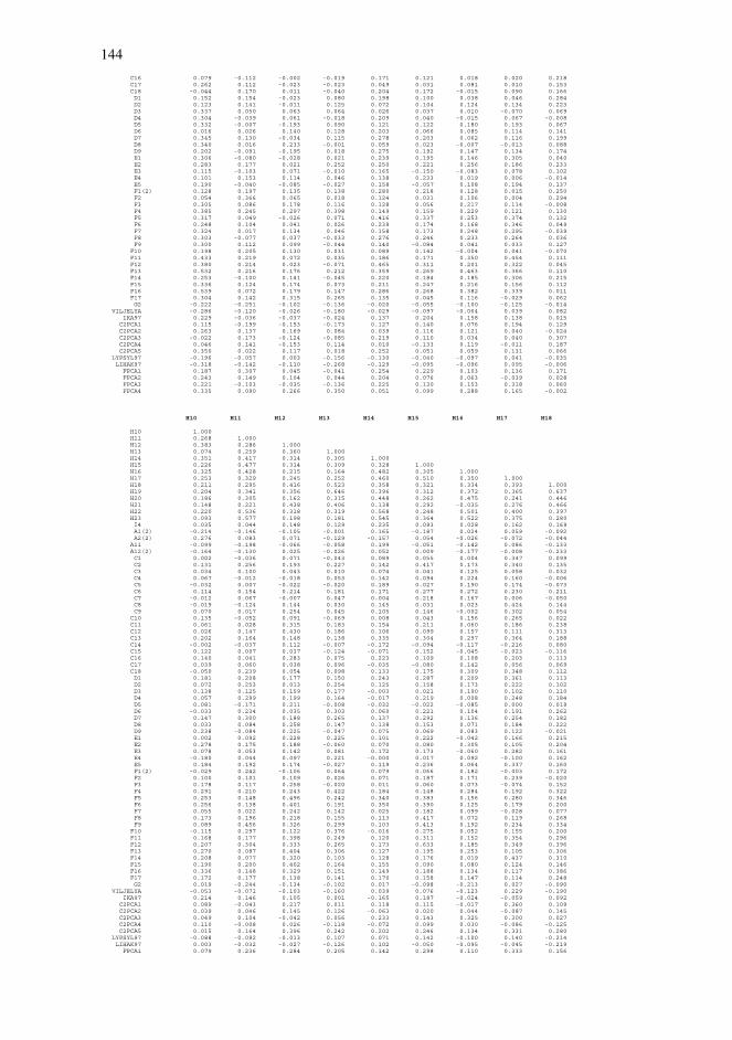
144 C16 0.079 -0.112 -0.002 -0.019 0.171 0.121 0.018 0.020 0.218 C17 0.262 0.112 -0.023 -0.023 0.049 0.031 0.081 0.010 0.153 C18 -0.044 0.170 0.011 -0.040 0.204 0.172 -0.015 0.090 0.166 D1 0.152 0.154 -0.023 0.080 0.198 0.100 0.038 0.046 0.284 D2 0.123 0.141 -0.011 0.125 0.072 0.104 0.124 0.134 0.223 D3 0.337 0.050 0.063 0.064 0.026 0.037 0.010 -0.070 0.069 D4 0.304 -0.039 0.061 -0.018 0.209 0.040 -0.015 0.067 -0.008 D5 0.332 -0.007 -0.193 0.090 0.121 0.122 0.180 0.193 0.067 D6 0.016 0.026 0.140 0.128 0.203 0.066 0.085 0.114 0.141 D7 0.345 0.130 -0.034 0.115 0.278 0.203 0.062 0.116 0.199 D8 0.340 0.016 0.233 -0.001 0.059 0.023 -0.007 -0.013 0.088 D9 0.202 -0.091 -0.195 0.018 0.275 0.192 0.147 0.134 0.174 E1 0.306 -0.080 -0.028 0.021 0.239 0.195 0.146 0.305 0.040 E2 0.283 0.177 0.021 0.252 0.250 0.221 0.256 0.186 0.233 E3 0.115 -0.103 0.071 -0.010 0.165 -0.150 -0.083 0.078 0.102 E4 0.101 0.153 0.114 0.046 0.138 0.233 0.019 0.006 -0.014 E5 0.190 -0.040 -0.085 -0.027 0.158 -0.057 0.108 0.194 0.137 F1(2) 0.128 0.197 0.135 0.138 0.280 0.218 0.128 0.015 0.250 F2 0.054 0.366 0.065 0.018 0.124 0.031 0.106 0.004 0.294 F3 0.305 0.086 0.178 0.116 0.128 0.056 0.217 0.114 -0.008 F4 0.385 0.245 0.297 0.398 0.149 0.159 0.229 0.121 0.130 F5 0.317 0.049 -0.026 0.071 0.416 0.337 0.253 0.374 0.132 F6 0.248 0.104 0.041 0.026 0.239 0.174 0.168 0.346 0.049 F7 0.324 0.017 0.134 0.046 0.158 0.173 0.248 0.295 -0.039 F8 0.303 -0.077 0.037 -0.033 0.276 0.246 0.233 0.264 0.036 F9 0.300 0.112 0.099 -0.044 0.140 -0.084 0.041 0.033 0.127 F10 0.198 0.205 0.130 0.031 0.089 0.142 -0.004 0.041 -0.070 F11 0.433 0.219 0.072 0.035 0.186 0.171 0.350 0.454 0.111 F12 0.380 0.214 0.023 -0.071 0.465 0.311 0.201 0.322 0.045 F13 0.532 0.216 0.176 0.212 0.359 0.269 0.463 0.366 0.110 F14 0.253 -0.100 0.141 -0.045 0.220 0.184 0.185 0.306 0.215 F15 0.336 0.124 0.174 0.073 0.211 0.247 0.216 0.156 0.112 F16 0.539 0.072 0.179 0.147 0.286 0.268 0.382 0.339 0.011 F17 0.304 0.142 0.315 0.265 0.135 0.045 0.116 -0.029 0.062 G2 -0.222 -0.251 -0.102 -0.136 -0.020 -0.055 -0.100 -0.125 -0.014 VILJELYA -0.286 -0.120 -0.026 -0.180 -0.029 -0.097 -0.064 0.039 0.082 IKA97 0.229 -0.036 -0.037 -0.024 0.137 0.204 0.158 0.138 0.015 C2PCA1 0.115 -0.199 -0.153 -0.173 0.127 0.140 0.076 0.194 0.129 C2PCA2 0.263 0.137 0.169 0.084 0.039 0.116 0.121 0.040 -0.024 C2PCA3 -0.022 0.173 -0.124 -0.085 0.219 0.110 0.034 0.040 0.307 C2PCA4 0.046 0.141 -0.153 0.114 0.010 -0.133 0.119 -0.011 0.187 C2PCA5 0.350 0.022 0.117 0.018 0.252 0.051 0.059 0.131 0.066 LYPSYL97 -0.196 -0.057 0.003 -0.156 -0.130 -0.040 -0.097 0.041 -0.035 LIHAK97 -0.318 -0.142 -0.110 -0.268 -0.129 -0.095 -0.096 0.095 -0.006 FPCA1 0.187 0.307 0.045 -0.041 0.254 0.229 0.103 0.136 0.171 FPCA2 0.243 0.149 0.104 0.044 0.204 0.076 0.063 -0.039 0.028 FPCA3 0.221 -0.103 -0.035 -0.136 0.225 0.130 0.153 0.318 0.060 FPCA4 0.335 0.090 0.266 0.350 0.051 0.099 0.288 0.165 -0.002

H10 H11 H12 H13 H14 H15 H16 H17 H18

H10 1.000 H11 0.268 1.000 H12 0.383 0.286 1.000 H13 0.074 0.259 0.360 1.000 H14 0.351 0.417 0.314 0.305 1.000 H15 0.226 0.477 0.314 0.309 0.328 1.000 H16 0.325 0.428 0.215 0.164 0.482 0.305 1.000 H17 0.253 0.329 0.245 0.252 0.460 0.510 0.350 1.000 H18 0.211 0.295 0.416 0.523 0.358 0.321 0.334 0.393 1.000 H19 0.204 0.341 0.356 0.646 0.396 0.312 0.372 0.365 0.637 H20 0.186 0.305 0.162 0.315 0.448 0.262 0.475 0.241 0.446 H21 0.148 0.221 0.438 0.406 0.138 0.292 -0.035 0.276 0.466 H22 0.220 0.536 0.318 0.319 0.568 0.248 0.501 0.400 0.397 H23 0.093 0.577 0.198 0.181 0.545 0.364 0.522 0.375 0.280 I4 0.035 0.044 0.148 0.129 0.235 0.093 0.028 0.162 0.169 A1(2) -0.214 -0.146 -0.105 -0.001 0.165 -0.187 0.024 0.059 -0.092 A2(2) 0.276 0.083 0.071 -0.129 -0.157 0.054 -0.026 -0.072 -0.044 A11 -0.099 -0.198 -0.066 -0.058 0.199 -0.051 -0.142 0.086 -0.133 A12(2) -0.164 -0.130 0.025 -0.026 0.052 0.009 -0.177 -0.008 -0.233 C1 0.002 -0.036 0.071 -0.043 0.089 0.055 0.004 0.347 0.099 C2 0.131 0.256 0.193 0.227 0.142 0.417 0.173 0.340 0.135 C3 0.034 0.100 0.043 0.010 0.074 0.041 0.125 0.058 0.032 C4 0.067 -0.012 -0.018 0.053 0.142 0.094 0.224 0.160 -0.006 C5 -0.032 0.007 -0.022 -0.020 0.189 0.027 0.190 0.174 -0.073 C6 0.114 0.154 0.214 0.181 0.171 0.277 0.272 0.230 0.211 C7 -0.012 0.067 -0.007 0.047 0.004 0.218 0.167 0.006 -0.050 C8 -0.019 -0.124 0.144 0.030 0.145 0.031 0.023 0.424 0.144 C9 0.070 0.017 0.254 0.045 0.105 0.146 -0.002 0.302 0.054 C10 0.135 -0.052 0.091 -0.069 0.008 0.043 0.156 0.265 0.022 C11 0.061 0.028 0.315 0.183 0.154 0.211 0.060 0.186 0.238 C12 0.026 0.147 0.430 0.186 0.106 0.099 0.157 0.111 0.313 C13 0.202 0.164 0.148 0.138 0.335 0.304 0.297 0.364 0.188 C14 -0.002 -0.037 0.112 -0.007 -0.172 -0.094 -0.117 -0.216 0.080 C15 0.122 0.007 0.037 -0.124 -0.071 0.152 -0.045 -0.023 -0.116 C16 0.140 0.041 0.283 0.075 0.223 0.109 0.108 0.203 0.113 C17 0.039 0.060 0.038 0.096 -0.035 -0.080 0.142 0.056 0.069 C18 -0.050 0.239 0.054 0.098 0.133 0.175 0.309 0.348 0.112 D1 0.181 0.208 0.177 0.150 0.243 0.287 0.209 0.361 0.113 D2 0.072 0.253 0.013 0.254 0.125 0.158 0.173 0.222 0.102 D3 0.138 0.125 0.159 0.177 -0.003 0.021 0.190 0.102 0.110 D4 0.057 0.299 0.199 0.164 -0.017 0.219 0.008 0.248 0.184 D5 0.081 -0.171 0.211 -0.008 -0.032 -0.022 -0.085 0.000 0.019 D6 -0.033 0.234 0.035 0.303 0.060 0.221 0.104 0.191 0.262 D7 0.147 0.300 0.188 0.265 0.137 0.292 0.136 0.254 0.182 D8 0.033 0.084 0.258 0.147 0.138 0.153 0.071 0.184 0.222 D9 0.238 -0.084 0.225 -0.047 0.075 0.069 0.083 0.122 -0.021 E1 0.002 0.092 0.228 0.225 0.101 0.222 -0.042 0.166 0.215 E2 0.278 0.175 0.188 -0.060 0.070 0.080 0.305 0.105 0.204 E3 0.078 0.053 0.142 0.081 0.172 0.173 -0.060 0.282 0.161 E4 -0.180 0.044 0.097 0.221 -0.000 0.017 0.092 -0.100 0.162 E5 0.184 0.192 0.174 -0.027 0.119 0.236 0.064 0.337 0.160 F1(2) -0.029 0.242 -0.106 0.064 0.079 0.066 0.182 -0.003 0.172 F2 0.100 0.101 0.109 0.026 0.071 0.187 0.171 0.239 -0.020 F3 0.178 0.117 0.258 -0.020 0.011 0.060 0.073 -0.074 0.152 F4 0.291 0.210 0.243 0.422 0.184 0.148 0.284 0.192 0.322 F5 0.253 0.148 0.496 0.242 0.340 0.383 0.156 0.280 0.346 F6 0.256 0.138 0.401 0.191 0.350 0.390 0.125 0.179 0.200 F7 0.055 0.022 0.242 0.142 0.025 0.182 0.099 -0.028 0.077 F8 0.173 0.196 0.218 0.155 0.113 0.417 0.072 0.119 0.268 F9 0.089 0.456 0.326 0.299 0.103 0.413 0.192 0.234 0.334 F10 -0.115 0.297 0.122 0.376 -0.016 0.275 0.052 0.155 0.200 F11 0.168 0.177 0.398 0.249 0.120 0.311 0.152 0.354 0.296 F12 0.207 0.304 0.333 0.265 0.173 0.633 0.185 0.349 0.396 F13 0.270 0.087 0.404 0.306 0.127 0.195 0.253 0.105 0.306 F14 0.208 0.077 0.320 0.103 0.128 0.176 0.019 0.437 0.310 F15 0.190 0.200 0.402 0.164 0.155 0.090 0.080 0.124 0.146 F16 0.336 0.148 0.329 0.151 0.149 0.188 0.134 0.117 0.386 F17 0.172 0.177 0.138 0.141 0.170 0.158 0.147 0.114 0.248 G2 0.019 -0.244 -0.134 -0.102 0.017 -0.098 -0.213 0.027 -0.090 VILJELYA -0.053 -0.071 -0.103 -0.160 0.039 0.076 -0.123 0.229 -0.190 IKA97 0.214 0.146 0.105 0.001 -0.165 0.187 -0.024 -0.059 0.092 C2PCA1 0.089 -0.043 0.217 0.011 0.118 0.115 -0.017 0.360 0.109 C2PCA2 0.039 0.046 0.145 0.126 -0.063 0.020 0.044 -0.087 0.145 C2PCA3 0.049 0.104 -0.042 0.056 0.233 0.143 0.325 0.300 0.027 C2PCA4 0.110 -0.008 0.026 -0.118 -0.072 0.099 0.030 -0.086 -0.125 C2PCA5 0.015 0.164 0.396 0.242 0.202 0.246 0.134 0.331 0.280 LYPSYL97 -0.088 -0.092 -0.013 0.107 0.071 0.142 -0.100 0.140 -0.214 LIHAK97 0.003 -0.032 -0.027 -0.126 0.102 -0.050 -0.095 -0.045 -0.219 FPCA1 0.079 0.236 0.284 0.205 0.142 0.298 0.110 0.333 0.156

145 FPCA2 -0.026 0.391 0.037 0.144 -0.008 0.232 0.133 -0.021 0.279 FPCA3 0.135 0.126 0.311 0.158 0.117 0.408 0.055 0.253 0.248 FPCA4 0.257 -0.073 0.166 0.100 0.121 -0.112 0.138 -0.069 0.120

H19 H20 H21 H22 H23 I4 A1(2) A2(2) A11

H19 1.000 H20 0.420 1.000 H21 0.359 0.089 1.000 H22 0.450 0.294 0.213 1.000 H23 0.226 0.440 0.125 0.629 1.000 I4 -0.012 0.170 -0.098 0.062 0.082 1.000 A1(2) -0.035 0.104 -0.048 0.012 0.086 -0.044 1.000 A2(2) -0.046 -0.179 -0.028 -0.070 -0.177 0.143 -0.725 1.000 A11 0.026 0.005 -0.273 -0.047 0.038 0.027 0.138 -0.146 1.000 A12(2) -0.107 -0.000 -0.247 -0.093 -0.048 -0.007 -0.005 -0.190 0.594 C1 0.083 0.056 0.133 0.104 0.042 0.098 0.007 0.008 0.152 C2 0.208 0.081 0.367 0.200 0.161 -0.018 -0.225 0.124 -0.070 C3 0.056 0.112 -0.083 -0.063 0.160 -0.007 0.036 -0.041 -0.003 C4 0.258 0.122 -0.054 0.065 -0.019 0.046 0.109 -0.038 0.131 C5 0.164 0.014 -0.071 0.112 0.021 0.090 0.101 -0.075 0.228 C6 0.318 0.254 0.066 0.159 0.135 -0.116 -0.034 -0.238 0.121 C7 0.125 0.113 -0.152 0.115 0.048 0.015 0.058 -0.092 -0.141 C8 0.091 0.028 0.158 0.146 0.081 0.115 0.084 -0.037 0.365 C9 0.070 -0.021 0.179 0.237 0.082 0.085 -0.095 0.114 0.096 C10 0.122 -0.100 0.049 0.028 -0.125 0.054 0.189 -0.017 -0.003 C11 0.275 0.204 0.224 0.168 0.146 0.049 0.068 -0.152 0.201 C12 0.272 0.112 0.233 0.210 0.084 0.023 -0.200 0.048 0.072 C13 0.286 0.201 0.190 0.248 0.229 0.165 0.060 -0.052 0.084 C14 0.087 -0.004 0.130 -0.113 -0.201 -0.103 0.094 -0.045 -0.213 C15 -0.050 -0.186 -0.006 -0.058 0.029 -0.197 0.070 0.038 -0.021 C16 0.107 0.010 0.080 0.213 0.151 0.125 0.050 -0.027 0.175 C17 0.205 0.103 0.134 0.026 0.062 0.013 -0.022 0.076 -0.064 C18 0.221 0.016 0.057 0.318 0.190 0.110 -0.189 0.132 -0.068 D1 0.276 -0.007 0.058 0.234 0.254 -0.034 0.009 -0.010 0.143 D2 0.297 -0.015 0.027 0.137 0.088 -0.062 -0.237 0.252 -0.040 D3 0.260 0.015 0.043 0.084 0.108 -0.067 -0.126 0.145 -0.137 D4 0.181 -0.030 0.214 0.172 0.056 0.117 -0.420 0.275 -0.145 D5 0.158 -0.190 0.075 -0.102 -0.183 -0.115 -0.107 0.122 -0.131 D6 0.221 0.235 0.038 0.129 0.244 -0.007 -0.222 -0.003 -0.090 D7 0.295 0.124 0.151 0.096 0.275 0.016 -0.253 0.145 -0.009 D8 0.251 0.212 0.090 0.135 0.182 0.024 -0.123 0.021 0.081 D9 -0.019 -0.028 0.084 0.000 -0.038 0.007 -0.099 0.062 0.068 E1 0.171 0.122 0.304 0.044 0.118 0.249 -0.222 0.104 0.000 E2 0.151 0.206 0.018 0.256 0.237 -0.069 -0.021 0.001 0.003 E3 0.021 0.137 0.242 0.108 0.066 0.188 -0.201 0.187 -0.051 E4 0.367 0.023 0.083 0.045 0.004 -0.068 -0.223 0.130 0.029 E5 0.016 0.063 0.194 0.143 0.129 0.215 -0.115 0.165 -0.079 F1(2) 0.203 0.087 0.012 0.126 0.219 -0.065 -0.202 0.153 -0.129 F2 0.189 -0.046 -0.141 0.200 0.140 0.016 0.017 0.057 0.160 F3 0.028 0.166 0.110 0.110 0.173 -0.070 -0.039 0.050 -0.091 F4 0.386 0.382 0.027 0.240 0.163 0.152 -0.159 0.169 -0.127 F5 0.243 0.248 0.248 0.272 0.242 0.219 -0.155 0.094 0.058 F6 0.165 0.159 0.163 0.195 0.212 0.283 -0.146 0.073 0.161 F7 0.090 -0.047 0.076 0.014 0.029 0.150 -0.110 0.167 -0.006 F8 0.125 0.100 0.248 0.056 0.122 0.092 -0.208 0.204 -0.036 F9 0.316 0.056 0.312 0.231 0.187 0.062 -0.275 0.176 -0.134 F10 0.327 0.037 0.134 0.157 0.117 0.007 -0.243 0.162 -0.120 F11 0.237 0.145 0.339 0.216 0.151 0.096 -0.314 0.290 -0.015 F12 0.260 0.120 0.360 0.153 0.237 0.102 -0.317 0.222 -0.037 F13 0.268 0.177 0.261 0.130 0.155 0.122 -0.241 0.222 -0.070 F14 0.170 0.106 0.242 0.108 0.096 0.109 -0.243 0.146 0.203 F15 0.226 0.097 -0.030 0.273 0.103 -0.039 -0.061 0.019 0.080 F16 0.166 0.252 0.232 0.199 0.228 0.105 -0.276 0.192 -0.058 F17 0.130 0.279 0.010 0.121 0.236 0.031 -0.168 0.068 0.014 G2 -0.224 -0.231 -0.102 -0.217 -0.205 0.215 0.001 0.062 0.003 VILJELYA -0.193 -0.055 -0.155 0.048 0.113 0.013 -0.140 -0.019 0.396 IKA97 0.035 -0.104 0.048 -0.012 -0.086 0.044 -1.000 0.725 -0.138 C2PCA1 0.052 -0.043 0.215 0.152 0.064 0.065 0.013 0.030 0.211 C2PCA2 0.244 0.161 0.158 -0.035 -0.030 -0.132 0.048 -0.131 -0.071 C2PCA3 0.251 0.102 -0.015 0.165 0.090 0.141 0.056 -0.015 0.097 C2PCA4 -0.042 -0.095 -0.164 -0.077 -0.008 -0.107 0.153 -0.034 -0.122 C2PCA5 0.238 0.195 0.277 0.325 0.252 0.131 -0.233 0.067 0.140 LYPSYL97 0.046 0.025 -0.053 -0.044 -0.069 0.108 -0.063 0.027 0.279 LIHAK97 -0.151 -0.069 -0.142 -0.049 0.125 0.123 -0.007 -0.048 0.239 FPCA1 0.301 0.017 0.033 0.286 0.166 0.004 -0.136 0.076 0.115 FPCA2 0.186 0.109 0.225 0.132 0.220 -0.133 -0.251 0.158 -0.289 FPCA3 0.124 0.012 0.335 0.044 0.076 0.182 -0.206 0.175 0.055 FPCA4 0.054 0.277 -0.053 0.068 0.096 0.110 -0.040 0.063 -0.015

A12(2) C1 C2 C3 C4 C5 C6 C7 C8

A12(2) 1.000 C1 0.208 1.000 C2 0.132 0.399 1.000 C3 -0.065 -0.048 -0.104 1.000 C4 0.032 0.261 0.307 0.310 1.000 C5 0.152 0.273 0.223 0.369 0.738 1.000 C6 0.146 0.072 0.430 0.239 0.397 0.287 1.000 C7 -0.096 -0.119 0.062 0.146 0.271 0.124 0.325 1.000 C8 0.236 0.711 0.342 0.020 0.180 0.285 0.150 -0.179 1.000 C9 0.114 0.311 0.224 0.258 0.323 0.310 0.143 0.100 0.438 C10 -0.040 0.467 0.170 0.237 0.527 0.428 0.189 0.254 0.403 C11 0.184 0.239 0.320 0.288 0.346 0.317 0.426 -0.091 0.276 C12 0.082 0.186 0.259 0.243 0.200 0.298 0.376 -0.136 0.308 C13 -0.099 0.264 0.333 0.379 0.691 0.679 0.353 0.211 0.296 C14 -0.113 0.110 -0.058 0.282 0.218 0.228 0.213 -0.015 0.037 C15 0.067 0.081 0.125 0.178 0.209 0.109 0.074 0.087 0.033 C16 0.137 0.404 0.346 0.081 0.264 0.323 0.155 -0.124 0.477 C17 -0.238 0.026 0.151 0.355 0.404 0.309 0.313 0.252 0.062 C18 0.028 0.355 0.367 -0.006 0.309 0.331 0.247 0.058 0.205 D1 -0.002 0.351 0.454 0.169 0.468 0.461 0.282 0.134 0.330 D2 -0.030 -0.037 0.258 0.135 0.230 0.196 0.139 0.086 -0.019 D3 -0.187 -0.073 0.091 0.061 0.090 -0.008 0.054 0.161 -0.046 D4 -0.043 0.170 0.278 0.029 0.217 0.153 0.110 -0.077 0.124 D5 -0.124 0.121 0.068 0.347 0.279 0.228 0.120 0.048 0.166 D6 0.115 0.043 0.073 0.215 0.020 0.031 0.180 0.038 -0.058 D7 0.017 0.002 0.340 0.156 0.132 0.124 0.144 0.028 0.050 D8 -0.018 0.158 0.198 0.111 0.222 0.211 0.231 -0.093 0.120 D9 0.091 0.222 0.258 0.201 0.203 0.450 0.097 -0.149 0.318 E1 0.157 0.086 0.108 0.189 0.111 0.152 -0.020 -0.166 0.130 E2 -0.193 0.075 0.075 0.079 0.088 -0.034 0.154 0.169 0.056 E3 0.111 0.215 0.309 0.063 0.154 0.060 0.178 0.015 0.304 E4 0.143 0.121 0.163 -0.036 0.241 0.252 0.308 0.010 0.001 E5 -0.209 0.128 0.146 0.166 0.254 0.253 0.081 -0.019 0.187 F1(2) -0.101 0.087 0.181 0.015 0.160 0.106 0.118 0.027 0.046 F2 0.153 0.179 0.304 0.184 0.617 0.387 0.189 0.182 0.072 F3 -0.089 0.044 0.005 -0.048 -0.160 -0.221 0.022 0.161 0.037 F4 -0.139 0.159 0.156 0.006 0.165 0.037 0.154 0.150 0.050 F5 0.073 0.252 0.315 0.116 0.312 0.275 0.269 0.032 0.259 F6 0.149 0.268 0.295 0.253 0.199 0.298 0.211 0.094 0.208 F7 -0.011 0.205 0.188 0.286 0.259 0.299 0.047 -0.073 0.145 F8 0.020 0.246 0.494 0.011 0.221 0.098 0.182 -0.211 0.234 F9 -0.098 0.014 0.276 0.085 0.038 0.045 0.160 -0.130 0.024 F10 0.057 0.131 0.306 -0.135 0.013 0.038 0.012 0.058 0.034 F11 0.105 0.298 0.248 -0.011 -0.145 -0.149 0.085 -0.032 0.307 F12 0.042 0.303 0.470 -0.077 0.110 0.007 0.189 0.002 0.208 F13 -0.033 0.199 0.232 0.193 0.132 0.069 0.193 -0.045 0.097 F14 0.255 0.574 0.442 0.141 0.241 0.336 0.165 -0.270 0.596

146 F15 0.077 0.156 0.150 -0.016 0.196 0.145 0.213 -0.019 0.085 F16 -0.173 0.192 0.096 -0.024 -0.067 -0.176 0.063 -0.190 0.175 F17 -0.097 -0.077 -0.018 0.007 -0.060 -0.150 0.122 -0.101 -0.048 G2 0.040 0.201 0.045 0.046 -0.068 -0.107 -0.190 0.014 0.115 VILJELYA 0.670 0.363 0.269 -0.049 -0.019 0.073 0.050 -0.137 0.376 IKA97 0.005 -0.007 0.225 -0.036 -0.109 -0.101 0.034 -0.058 -0.084 C2PCA1 0.246 0.803 0.518 -0.131 0.157 0.182 0.106 -0.221 0.827 C2PCA2 -0.053 0.026 0.232 0.310 0.343 0.274 0.633 0.129 0.016 C2PCA3 -0.016 0.248 0.268 0.346 0.827 0.824 0.301 0.207 0.180 C2PCA4 -0.108 -0.143 -0.185 0.534 0.269 0.139 0.112 0.562 -0.139 C2PCA5 0.140 0.199 0.360 0.311 0.142 0.200 0.314 0.007 0.368 LYPSYL97 0.616 0.213 0.269 0.092 0.076 0.103 0.057 0.093 0.299 LIHAK97 0.478 0.189 0.156 0.095 0.173 0.154 0.093 -0.033 0.196 FPCA1 0.192 0.245 0.340 -0.031 0.345 0.249 0.198 0.096 0.139 FPCA2 -0.226 -0.122 0.088 -0.220 -0.270 -0.338 0.028 -0.003 -0.117 FPCA3 0.134 0.348 0.471 0.181 0.231 0.279 0.152 -0.189 0.356 FPCA4 -0.140 0.021 -0.171 0.109 -0.072 -0.114 0.025 0.038 -0.005

C9 C10 C11 C12 C13 C14 C15 C16 C17

C9 1.000 C10 0.281 1.000 C11 0.242 0.178 1.000 C12 0.310 0.154 0.482 1.000 C13 0.238 0.523 0.406 0.291 1.000 C14 0.041 0.234 0.371 0.203 0.115 1.000 C15 0.235 0.276 0.123 0.019 0.082 0.239 1.000 C16 0.327 0.337 0.245 0.324 0.325 0.082 0.209 1.000 C17 0.066 0.398 0.180 0.227 0.424 0.221 0.100 0.100 1.000 C18 0.176 0.279 0.037 0.103 0.315 0.046 -0.057 0.104 0.153 D1 0.344 0.256 0.290 0.287 0.455 0.007 0.312 0.523 0.065 D2 0.022 0.107 0.056 0.135 0.210 0.062 0.037 -0.154 0.399 D3 -0.088 0.199 0.146 0.162 0.168 -0.079 0.066 -0.069 0.311 D4 0.319 0.066 0.321 0.268 0.271 0.035 -0.059 0.057 0.060 D5 0.466 0.251 0.250 0.335 0.163 0.273 0.259 0.223 0.112 D6 0.109 -0.240 0.043 0.105 -0.009 0.025 -0.135 -0.199 0.167 D7 0.094 -0.051 0.163 0.165 0.239 -0.090 0.071 -0.059 0.307 D8 0.112 -0.029 0.627 0.403 0.273 0.234 -0.160 0.132 0.119 D9 0.365 0.251 0.129 0.370 0.325 0.075 0.298 0.490 0.033 E1 0.291 0.018 0.333 0.248 0.183 0.164 0.177 -0.024 0.171 E2 0.001 0.273 0.011 0.028 0.211 -0.085 0.110 0.236 0.144 E3 0.315 -0.040 0.190 0.232 0.185 -0.066 0.027 0.071 -0.049 E4 -0.030 -0.095 0.336 0.420 0.062 0.261 -0.034 0.003 0.204 E5 0.360 0.250 0.146 0.061 0.360 0.151 0.233 0.083 0.073 F1(2) -0.056 0.007 0.051 0.315 0.108 0.056 0.018 0.145 0.262 F2 0.253 0.380 0.466 0.182 0.413 0.057 0.209 0.273 0.130 F3 0.097 0.042 0.210 0.144 -0.077 0.076 -0.114 0.035 0.049 F4 -0.009 0.058 0.294 0.156 0.182 0.136 -0.112 0.019 0.120 F5 0.372 0.155 0.405 0.328 0.426 0.180 0.087 0.266 0.004 F6 0.285 0.163 0.465 0.321 0.421 0.179 0.115 0.211 0.044 F7 0.157 0.282 0.412 0.347 0.280 0.294 0.153 0.184 0.178 F8 0.251 0.070 0.300 0.195 0.222 0.213 0.161 0.211 -0.007 F9 0.118 -0.093 0.102 0.332 0.056 0.151 0.069 -0.019 0.022 F10 0.010 -0.164 -0.022 0.102 -0.118 0.062 -0.025 -0.079 0.023 F11 0.383 -0.006 0.163 0.230 -0.143 0.031 0.031 -0.026 0.022 F12 0.190 0.157 0.189 0.257 0.190 0.013 0.192 0.174 0.013 F13 0.188 0.199 0.462 0.497 0.202 0.255 0.188 0.137 0.276 F14 0.358 0.153 0.362 0.420 0.340 0.040 0.027 0.432 0.078 F15 0.098 -0.027 0.429 0.282 0.083 0.123 -0.040 0.175 -0.039 F16 0.120 -0.058 0.376 0.339 0.062 0.183 0.004 0.103 0.020 F17 -0.109 -0.268 0.231 0.307 0.026 0.006 -0.160 -0.067 -0.065 G2 0.031 0.193 -0.302 -0.252 -0.040 -0.191 -0.022 0.084 -0.050 VILJELYA 0.264 -0.043 0.121 0.039 -0.077 -0.219 0.089 0.273 -0.253 IKA97 0.095 -0.189 -0.068 0.200 -0.060 -0.094 -0.070 -0.050 0.022 C2PCA1 0.464 0.424 0.236 0.268 0.186 0.049 0.269 0.729 -0.023 C2PCA2 -0.068 0.189 0.569 0.301 0.260 0.750 0.194 0.113 0.595 C2PCA3 0.195 0.540 0.254 0.163 0.833 0.085 -0.029 0.133 0.372 C2PCA4 0.294 0.433 -0.033 -0.043 0.179 0.237 0.692 0.116 0.241 C2PCA5 0.638 0.009 0.562 0.706 0.285 -0.123 -0.161 0.168 0.117 LYPSYL97 0.275 0.018 0.091 -0.003 -0.024 -0.117 -0.022 0.092 0.010 LIHAK97 0.192 0.042 0.082 -0.039 0.075 -0.016 0.155 0.085 0.015 FPCA1 0.204 0.096 0.302 0.214 0.181 0.004 0.103 0.195 -0.004 FPCA2 -0.119 -0.265 -0.197 0.141 -0.286 0.007 -0.070 -0.155 0.035 FPCA3 0.365 0.215 0.269 0.278 0.334 0.176 0.207 0.269 0.054 FPCA4 -0.040 0.001 0.335 0.197 0.061 0.132 -0.129 -0.025 0.090

C18 D1 D2 D3 D4 D5 D6 D7 D8

C18 1.000 D1 0.298 1.000 D2 0.457 0.171 1.000 D3 0.100 0.136 0.457 1.000 D4 0.265 0.256 0.253 0.247 1.000 D5 -0.061 0.398 0.190 0.161 0.368 1.000 D6 0.258 -0.071 0.502 0.156 0.252 0.036 1.000 D7 0.168 0.203 0.626 0.414 0.342 0.265 0.585 1.000 D8 0.115 0.285 0.147 0.312 0.447 0.218 0.183 0.269 1.000 D9 0.049 0.477 0.000 -0.020 0.018 0.447 -0.146 0.139 0.048 E1 0.011 0.034 0.225 0.017 0.370 0.311 0.270 0.357 0.211 E2 0.219 0.218 -0.010 0.049 0.005 0.055 -0.147 0.186 0.017 E3 0.115 0.222 0.072 0.047 0.454 0.289 0.192 0.186 0.220 E4 0.214 0.167 0.246 0.215 0.233 0.183 0.317 0.264 0.449 E5 0.233 0.203 0.138 -0.037 0.502 0.221 0.032 0.105 0.146 F1(2) 0.203 0.110 0.167 0.148 0.081 -0.077 0.189 0.193 0.206 F2 0.305 0.531 0.202 0.187 0.253 0.187 -0.094 0.176 0.355 F3 0.034 0.058 0.029 0.025 0.039 0.055 0.053 0.057 0.274 F4 0.191 0.287 0.172 0.210 0.280 0.079 0.130 0.196 0.503 F5 0.357 0.376 0.151 -0.001 0.272 0.153 0.059 0.134 0.325 F6 0.223 0.355 0.055 -0.041 0.232 0.178 -0.040 0.128 0.380 F7 0.136 0.294 0.143 0.010 0.227 0.345 -0.078 0.044 0.277 F8 0.179 0.236 0.173 -0.045 0.363 0.177 0.150 0.202 0.267 F9 0.263 0.150 0.303 0.009 0.316 0.118 0.272 0.192 0.214 F10 0.296 0.223 0.380 0.044 0.222 0.002 0.338 0.274 0.103 F11 0.240 -0.020 0.172 -0.110 0.224 0.145 0.254 0.243 0.095 F12 0.437 0.377 0.266 0.056 0.216 0.030 0.143 0.234 0.156 F13 0.169 0.180 0.188 0.218 0.197 0.270 0.042 0.184 0.323 F14 0.330 0.479 0.170 -0.037 0.381 0.225 0.167 0.224 0.288 F15 0.098 0.264 0.027 0.077 0.241 0.086 0.006 0.073 0.448 F16 0.125 0.148 -0.023 0.017 0.254 0.104 -0.006 0.092 0.433 F17 0.184 0.174 0.114 0.140 0.209 -0.006 0.089 0.120 0.451 G2 0.009 -0.033 -0.046 -0.129 -0.093 0.024 -0.065 -0.056 -0.261 VILJELYA 0.198 0.238 -0.076 -0.226 0.000 -0.050 0.114 -0.010 -0.051 IKA97 0.189 -0.009 0.237 0.126 0.420 0.107 0.222 0.253 0.123 C2PCA1 0.184 0.445 -0.121 -0.096 0.128 0.206 -0.141 -0.008 0.074 C2PCA2 0.063 0.091 0.211 0.100 0.058 0.166 0.139 0.141 0.349 C2PCA3 0.563 0.399 0.347 0.139 0.250 0.114 0.074 0.191 0.203 C2PCA4 -0.190 0.185 -0.030 0.098 -0.152 0.343 -0.116 -0.041 -0.233 C2PCA5 0.150 0.277 0.134 0.125 0.414 0.314 0.255 0.280 0.444 LYPSYL97 0.111 0.031 0.155 -0.006 -0.045 0.054 0.245 0.204 -0.108 LIHAK97 0.045 0.093 -0.038 -0.091 -0.059 -0.088 0.063 -0.006 -0.081 FPCA1 0.362 0.435 0.223 0.097 0.242 0.040 0.085 0.208 0.261 FPCA2 0.140 -0.141 0.198 0.040 0.035 -0.167 0.320 0.160 0.043 FPCA3 0.262 0.311 0.209 -0.094 0.315 0.265 0.123 0.170 0.116 FPCA4 -0.066 0.031 -0.101 0.112 0.074 0.116 -0.113 -0.010 0.408

D9 E1 E2 E3 E4 E5 F1(2) F2 F3

D9 1.000 E1 0.257 1.000

147 E2 0.174 -0.015 1.000 E3 0.197 0.368 -0.031 1.000 E4 -0.084 0.169 -0.136 0.103 1.000 E5 0.254 0.349 0.252 0.315 -0.156 1.000 F1(2) -0.068 -0.012 0.076 0.019 0.398 -0.139 1.000 F2 0.092 0.011 0.236 0.060 0.227 0.058 0.188 1.000 F3 -0.053 -0.039 0.408 0.000 0.054 0.006 0.252 0.104 1.000 F4 -0.111 0.085 0.215 0.061 0.305 0.070 0.180 0.270 0.391 F5 0.296 0.354 0.200 0.334 0.126 0.360 0.107 0.360 0.229 F6 0.347 0.312 0.173 0.199 0.111 0.331 0.069 0.328 0.256 F7 0.319 0.412 0.078 0.060 0.136 0.247 0.109 0.286 0.215 F8 0.257 0.343 0.026 0.255 0.060 0.399 0.226 0.133 0.182 F9 0.096 0.333 -0.109 0.225 0.112 0.251 0.143 -0.014 -0.062 F10 -0.076 0.252 -0.178 0.094 0.310 -0.013 0.208 0.111 0.027 F11 0.023 0.449 0.130 0.253 0.192 0.104 0.042 -0.002 0.236 F12 0.118 0.307 0.191 0.103 0.233 0.196 0.197 0.264 0.201 F13 0.263 0.445 0.189 0.066 0.340 0.108 0.265 0.277 0.254 F14 0.408 0.366 0.135 0.400 0.126 0.290 0.094 0.262 0.078 F15 -0.005 0.077 0.167 0.029 0.328 0.050 0.144 0.443 0.245 F16 0.059 0.223 0.327 0.121 0.241 0.190 0.271 0.164 0.518 F17 -0.086 0.036 0.264 0.221 0.287 0.048 0.380 0.195 0.410 G2 0.029 -0.059 0.019 0.096 -0.437 -0.002 -0.129 -0.135 -0.055 VILJELYA 0.237 0.059 -0.055 0.254 0.028 -0.039 0.018 0.232 0.005 IKA97 0.099 0.222 0.021 0.201 0.223 0.115 0.202 -0.017 0.039 C2PCA1 0.420 0.083 0.120 0.240 -0.013 0.162 0.068 0.153 0.045 C2PCA2 0.018 0.157 0.011 -0.022 0.409 0.053 0.176 0.144 0.083 C2PCA3 0.222 0.102 0.130 0.100 0.158 0.311 0.120 0.508 -0.172 C2PCA4 0.172 0.028 0.188 -0.060 -0.192 0.166 -0.058 0.192 0.001 C2PCA5 0.226 0.329 -0.005 0.391 0.224 0.147 0.117 0.253 0.243 LYPSYL97 0.085 0.218 -0.298 0.218 0.096 -0.259 -0.139 0.118 -0.143 LIHAK97 -0.013 0.073 -0.260 0.124 0.052 -0.075 -0.119 0.182 -0.156 FPCA1 0.011 0.133 0.097 0.089 0.352 0.022 0.157 0.663 -0.017 FPCA2 -0.252 0.012 0.018 0.002 0.222 -0.101 0.625 -0.248 0.383 FPCA3 0.451 0.487 -0.036 0.313 -0.053 0.436 -0.060 0.089 -0.059 FPCA4 -0.021 0.033 0.340 0.004 0.175 0.008 0.141 0.123 0.572

F4 F5 F6 F7 F8 F9 F10 F11 F12

F4 1.000 F5 0.270 1.000 F6 0.309 0.660 1.000 F7 0.288 0.462 0.644 1.000 F8 0.086 0.497 0.462 0.539 1.000 F9 0.081 0.192 0.129 0.298 0.492 1.000 F10 0.279 0.278 0.097 0.302 0.309 0.543 1.000 F11 0.291 0.288 0.268 0.189 0.205 0.330 0.340 1.000 F12 0.273 0.571 0.452 0.328 0.449 0.357 0.437 0.503 1.000 F13 0.429 0.388 0.557 0.585 0.298 0.211 0.110 0.530 0.469 F14 0.262 0.537 0.429 0.379 0.422 0.266 0.309 0.402 0.447 F15 0.471 0.436 0.251 0.236 0.054 0.049 0.370 0.246 0.238 F16 0.539 0.478 0.491 0.376 0.309 0.110 0.114 0.469 0.517 F17 0.466 0.271 0.196 0.020 0.058 0.222 0.102 0.221 0.316 G2 -0.169 -0.104 -0.041 -0.045 0.060 -0.092 -0.129 -0.090 -0.072 VILJELYA -0.162 0.107 0.140 -0.016 0.072 -0.091 0.022 0.188 0.185 IKA97 0.159 0.155 0.146 0.110 0.208 0.275 0.243 0.314 0.317 C2PCA1 0.026 0.266 0.216 0.164 0.340 0.035 0.055 0.290 0.323 C2PCA2 0.208 0.156 0.184 0.252 0.203 0.139 0.072 0.026 0.052 C2PCA3 0.152 0.333 0.284 0.267 0.137 0.070 0.012 -0.154 0.141 C2PCA4 -0.089 0.002 0.083 0.100 -0.109 -0.093 -0.187 -0.093 -0.045 C2PCA5 0.187 0.400 0.416 0.261 0.222 0.250 0.103 0.428 0.261 LYPSYL97 -0.091 -0.005 0.080 -0.033 -0.002 -0.034 0.205 0.234 0.082 LIHAK97 -0.192 0.117 0.142 0.008 0.081 -0.079 0.005 -0.080 0.042 FPCA1 0.285 0.525 0.247 0.148 0.057 0.137 0.565 0.305 0.533 FPCA2 0.068 -0.035 -0.213 -0.117 0.249 0.511 0.421 0.267 0.320 FPCA3 -0.057 0.527 0.549 0.628 0.806 0.560 0.300 0.283 0.469 FPCA4 0.678 0.148 0.400 0.281 -0.105 -0.286 -0.251 0.224 0.025

F13 F14 F15 F16 F17 G2 VILJELYA IKA97 C2PCA1

F13 1.000 F14 0.352 1.000 F15 0.290 0.317 1.000 F16 0.634 0.360 0.479 1.000 F17 0.354 0.202 0.371 0.645 1.000 G2 -0.201 0.042 -0.382 -0.242 -0.220 1.000 VILJELYA 0.005 0.393 0.027 0.046 0.046 0.084 1.000 IKA97 0.241 0.243 0.061 0.276 0.168 -0.001 0.140 1.000 C2PCA1 0.167 0.584 0.124 0.185 -0.138 0.183 0.434 -0.013 1.000 C2PCA2 0.334 0.083 0.202 0.167 0.068 -0.277 -0.193 -0.048 0.004 C2PCA3 0.096 0.274 0.094 -0.102 -0.020 -0.023 -0.032 -0.056 0.032 C2PCA4 0.076 -0.217 -0.132 -0.159 -0.229 0.080 -0.129 -0.153 -0.047 C2PCA5 0.402 0.461 0.277 0.331 0.268 -0.149 0.230 0.233 0.245 LYPSYL97 -0.026 0.197 -0.069 -0.227 -0.187 0.191 0.564 0.063 0.244 LIHAK97 -0.111 0.132 -0.066 -0.162 -0.170 0.137 0.495 0.007 0.198 FPCA1 0.227 0.406 0.769 0.287 0.248 -0.277 0.225 0.136 0.209 FPCA2 0.052 -0.121 0.010 0.245 0.406 -0.121 -0.126 0.251 -0.090 FPCA3 0.333 0.614 -0.119 0.115 -0.162 0.156 0.166 0.206 0.414 FPCA4 0.557 0.067 0.323 0.698 0.570 -0.161 -0.088 0.040 -0.080

C2PCA2 C2PCA3 C2PCA4 C2PCA5 LYPSYL97 LIHAK97 FPCA1 FPCA2 FPCA3

C2PCA2 1.000 C2PCA3 0.180 1.000 C2PCA4 0.153 0.078 1.000 C2PCA5 0.048 0.167 -0.106 1.000 LYPSYL97 -0.047 0.041 -0.024 0.254 1.000 LIHAK97 0.027 0.101 0.049 0.068 0.518 1.000 FPCA1 0.083 0.278 -0.046 0.263 0.173 0.120 1.000 FPCA2 0.038 -0.281 -0.165 0.030 -0.169 -0.239 0.004 1.000 FPCA3 0.131 0.261 -0.007 0.310 0.156 0.176 0.050 -0.043 1.000 FPCA4 0.160 -0.062 -0.018 0.218 -0.205 -0.214 -0.051 -0.079 -0.255

FPCA4

FPCA4 1.000

148

Appendix 8

Discriminant analysis for the adjustment decision

MULTIVARIATE TEST STATISTICS

WILKS' LAMBDA = 0.508 F-STATISTIC = 5.548 DF = 35,1112 PROB = 0.000

PILLAI TRACE = 0.578 F-STATISTIC = 5.003 DF = 35,1340 PROB = 0.000

HOTELLING-LAWLEY TRACE = 0.807 F-STATISTIC = 6.050 DF = 35,1312 PROB = 0.000

THETA = 0.364 S = 5, M = .5, N =131.0 PROB = 0.000

TEST OF RESIDUAL ROOTS

ROOTS 1 THROUGH 5 CHI-SQUARE STATISTIC = 181.647 DF = 35 PROB = 0.000

ROOTS 2 THROUGH 5 CHI-SQUARE STATISTIC = 60.321 DF = 24 PROB = 0.000

ROOTS 3 THROUGH 5 CHI-SQUARE STATISTIC = 25.889 DF = 15 PROB = 0.039

ROOTS 4 THROUGH 5 CHI-SQUARE STATISTIC = 8.515 DF = 8 PROB = 0.385

ROOTS 5 THROUGH 5 CHI-SQUARE STATISTIC = 1.043 DF = 3 PROB = 0.791

CANONICAL CORRELATIONS

1 2 3 4 5

0.603 0.347 0.250 0.166 0.062

DEPENDENT VARIABLE CANONICAL COEFFICIENTS STANDARDIZED BY CONDITIONAL (WITHIN GROUPS) STANDARD DEVIATIONS

1 2 3 4 5

IKA97 -0.248 -0.580 0.545 0.201 0.529 VILJELYA 0.474 0.051 0.236 -0.513 -0.169 C2PCA1 0.220 0.068 -0.259 0.214 0.673 A12(2) 0.469 0.172 0.341 0.194 0.147 G2 -0.143 0.319 -0.317 -0.147 0.628 FPCA3 0.198 0.108 -0.098 0.795 -0.364 TSUUNTAU -0.336 0.718 0.600 0.186 -0.031

CANONICAL LOADINGS (CORRELATIONS BETWEEN CONDITIONAL DEPENDENT VARIABLES AND DEPENDENT CANONICAL FACTORS)

1 2 3 4 5

IKA97 -0.194 -0.533 0.599 0.243 0.451 VILJELYA 0.646 0.215 0.405 -0.320 0.149 C2PCA1 0.409 0.181 -0.221 0.318 0.557 A12(2) 0.763 0.006 0.341 -0.011 0.068 G2 -0.167 0.425 -0.261 -0.128 0.594 FPCA3 0.229 0.133 -0.084 0.855 -0.083 TSUUNTAU -0.385 0.720 0.522 0.120 0.034

149

Appendix 9

Comparison of changes in objectives in relation to adjustmentinto the EU.

Comparison of changes in objectives for maintained farmers

Objective Mean in1998

Mean in1993

Diffe-rence

Risk(p)

Increasing farm size

Ensuring continuity

Improving quality of life

Increasing profit

Improving profit for capital

Avoiding losses

Increasing leisure

Expanding production

Improving quality of products

Increasing assets

Ensuring liquidity

Taking care of the environment

Increasing total incomes

Maintaining low degree of debt to assets

Increasing household spending

Obtaining new and bigger machinery and buildings

Reducing risk

Increasing supports

2.81(1.60)

4.19(1.75)

4.78(1.32)

4.31(1.46)

4.58(1.28)

5.32(1.21)

4.19(1.50)

2.82(1.51)

4.41(1.46)

3.29(1.54)

5.43(0.85)

4.93(1.07)

4.52(1.34)

4.50(1.68)

2.47(1.27)

2.28(1.36)

4.84(1.19)

4.78(1.43)

3.57(1.79)

4.88(1.54)

4.76(1.34)

4.72(1.26)

4.76(1.30)

5.64(0.75)

3.78(1.61)

3.62(1.59)

5.53(0.83)

3.61(1.55)

5.64(0.76)

5.09(1.01)

4.18(1.45)

5.19(1.13)

2.48(1.40)

2.66(1.33)

n.a.

n.a.

-0.91(1.84)-0.68

(1.95)0.17

(1.56)-0.42

(1.55)-0.21

(1.58)-0.24

(1.31)+0.45(1.58)-0.71

(1.66)-1.09

(1.62)-0.25

(1.69)-0.20

(0.98)-0.28

(1.30)+0.33(1.62)-0.65

(1.89)+0.10(1.59)-0.35

(1.64)-

-

0.000

0.000

0.183

0.001

0.099

0.023

0.000

0.000

0.000

0.013

0.013

0.221

0.013

0.000

0.451

0.007

-

-

Number of cases 167, scale from 1 to 6 (1=not important, 6=very important). N.a. means that the questionwas not asked in the 1993 survey. Means in 1998 and in 1993 are calculated with all cases. However, thedifference between objectives in 1993 and in 1993 is calculated in pairs, thus the distinction between mean in1998 and mean in 1993 differs from the column ‘difference’. Standard deviation is presented in parenthesis.T-test is used here as a standard measure to compare values. To test the hypothesis that the 1998 and 1993values have the same mean, the two-tailed test is used to calculate the p-values.

150

Comparison of changes in objectives for expanded farmers

Objective Mean in1998

Mean in1993

Diffe-rence

Risk(p)

Increasing farm size

Ensuring continuity

Improving quality of life

Increasing profit

Improving profit for capital

Avoiding losses

Increasing leisure

Expanding production

Improving quality of products

Increasing assets

Ensuring liquidity

Taking care of the environment

Increasing total incomes

Maintaining low degree of debt to assets

Increasing household spending

Obtaining new and bigger machinery and buildings

Reducing risk

Increasing supports

4.18(1.47)

4.68(1.63)

5.02(1.21)

4.56(1.41)

4.93(0.97)

5.60(0.85)

4.33(1.57)

3.91(1.44)

4.45(1.53)

3.48(1.62)

5.65(0.75)

4.94(1.18)

4.71(1.24)

4.33(1.53)

2.23(1.33)

2.97(1.48)

4.95(1.16)

4.73(1.30)

4.20(1.66)

4.98(1.52)

4.70(1.51)

4.88(1.21)

5.16(0.99)

5.55(0.96)

3.74(1.51)

4.37(1.46)

5.51(0.91)

3.64(1.61)

5.75(0.63)

5.31(0.86)

4.31(1.36)

5.03(1.14)

2.18(1.35)

2.77(1.46)

n.a.

n.a.

-0.03(1.80)-0.30

(1.79)+0.39(1.74)-0.28

(1.80)-0.17

(1.34)+0.04(1.07)+0.46(1.97)-0.42

(1.77)-1.09

(1.60)-0.19

(1.94)-0.08

(1.04)-0.29

(1.24)+0.34(1.63)-0.62

(1.70)+0.12(0.69)+0.16(1.77)

-

-

0.863

0.108

0.034

0.138

0.216

0.700

0.026

0.024

0.000

0.363

0.485

0.026

0.044

0.001

0.501

0.379

-

-

Number of cases 93, scale from 1 to 6 (1=not important, 6=very important). N.a. means that the question wasnot asked in the 1993 survey. Means in 1998 and in 1993 are calculated with all cases. However, thedifference between objectives in 1993 and in 1993 is calculated in pairs, thus the distinction between mean in1998 and mean in 1993 differs from the column ‘difference’. Standard deviation is presented in parenthesis.T-test is used here as a standard measure to compare values. To test the hypothesis that the 1998 and 1993values have the same mean, the two-tailed test is used to calculate the p-values.

151

Comparison of changes in objectives for reduced farmers

Objective Mean in1998

Mean in1993

Diffe-rence

Risk(p)

Increasing farm size

Ensuring continuity

Improving quality of life

Increasing profit

Improving profit for capital

Avoiding losses

Increasing leisure

Expanding production

Improving quality of products

Increasing assets

Ensuring liquidity

Taking care of the environment

Increasing total incomes

Maintaining low degree of debt to assets

Increasing household spending

Obtaining new and bigger machinery and buildings

Reducing risk

Increasing supports

1.27(0.65)

3.36(2.16)

4.27(2.01)

2.91(1.81)

3.64(1.96)

4.82(1.99)

5.27(1.91)

1.46(0.82)

3.55(2.42)

2.36(1.80)

5.36(1.50)

4.82(1.47)

3.46(1.86)

3.82(2.14)

2.36(1.29)

1.18(0.41)

4.55(1.97)

5.00(1.61)

2.07(1.39)

4.21(1.81)

5.00(1.30)

4.57(1.60)

5.14(1.10)

5.86(0.36)

3.43(1.72)

2.43(1.65)

5.36(0.84)

2.43(1.45)

5.86(0.36)

5.14(1.10)

4.64(1.55)

5.50(0.94)

1.71(0.91)

1.64(1.01)

n.a.

n.a.

-0.30(1.06)-0.10

(1.37)-0.90

(2.60)-1.70

(2.21)-1.40

(2.76)-1.20

(2.10)+1.30(2.58)-1.00

(1.25)-2.20

(2.35)0.00

(2.71)-0.60

(1.65)-0.30

(1.42)-1.40

(1.78)-1.80

(2.62)+0.50(1.43)-0.50

(1.01)-

-

0.394

0.823

0.302

0.038

0.143

0.104

0.146

0.032

0.016

1.000

0.279

0.520

0.034

0.058

0.299

0.177

-

-

Number of cases 11, scale from 1 to 6 (1=not important, 6=very important). N.a. means that the question wasnot asked in the 1993 survey. Means in 1998 and in 1993 are calculated with all cases. However, thedifference between objectives in 1993 and in 1993 is calculated in pairs, thus the distinction between mean in1998 and mean in 1993 differs from the column ‘difference’. Standard deviation is presented in parenthesis.T-test is used here as a standard measure to compare values. To test the hypothesis that the 1998 and 1993values have the same mean, the two-tailed test is used to calculate the p-values.

152

Comparison of changes in objectives for farmers changed production line

Objective Mean in1998

Mean in1993

Diffe-rence

Risk(p)

Increasing farm size

Ensuring continuity

Improving quality of life

Increasing profit

Improving profit for capital

Avoiding losses

Increasing leisure

Expanding production

Improving quality of products

Increasing assets

Ensuring liquidity

Taking care of the environment

Increasing total incomes

Maintaining low degree of debt to assets

Increasing household spending

Obtaining new and bigger machinery and buildings

Reducing risk

Increasing supports

2.81(1.75)

4.00(1.61)

5.05(0.92)

4.38(1.60)

4.52(1.33)

5.33(0.73)

4.10(1.64)

3.52(1.99)

4.43(1.66)

3.48(1.66)

5.48(0.75)

4.86(1.32)

4.71(1.19)

5.05(1.20)

2.19(1.25)

2.10(1.34)

4.95(1.07)

4.81(1.37)

3.20(1.83)

4.36(1.68)

4.80(1.53)

4.72(1.28)

4.52(1.30)

5.28(1.21)

4.00(1.56)

3.32(1.91)

5.16(1.14)

3.00(1.58)

5.52(0.71)

5.24(0.83)

4.08(1.55)

5.04(0.94)

2.16(1.11)

2.36(1.15)

2.81(1.75)

4.00(1.61)

-0.81(2.01)-0.48

(1.94)-0.05

(1.24)-0.33

(1.28)-0.19

(1.03)+0.10(1.38)+0.14(1.85)+0.19(2.34)-1.05

(1.77)+0.33(1.93)-0.05

(0.92)-0.43

(1.25)+0.48(1.47)+0.05(1.43)

0.00(1.32)-0.38

(1.50)n.a.

n.a.

0.396

0.274

0.863

0.246

0.407

0.754

0.727

0.713

0.014

0.438

0.815

0.131

0.153

0.880

1.00

0.258

-

-

Number of cases 21, scale from 1 to 6 (1=not important, 6=very important). N.a. means that the question wasnot asked in the 1993 survey. Means in 1998 and in 1993 are calculated with all cases. However, thedifference between objectives in 1993 and in 1993 is calculated in pairs, thus the distinction between mean in1998 and mean in 1993 differs from the column ‘difference’. Standard deviation is presented in parenthesis.T-test is used here as a standard measure to compare values. To test the hypothesis that the 1998 and 1993values have the same mean, the two-tailed test is used to calculate the p-values.

153

Comparison of changes in objectives for farmers introduced additional processingfor agricultural products

Objective Mean in1998

Mean in1993

Diffe-rence

Risk(p)

Increasing farm size

Ensuring continuity

Improving quality of life

Increasing profit

Improving profit for capital

Avoiding losses

Increasing leisure

Expanding production

Improving quality of products

Increasing assets

Ensuring liquidity

Taking care of the environment

Increasing total incomes

Maintaining low degree of debt to assets

Increasing household spending

Obtaining new and bigger machinery and buildings

Reducing risk

Increasing supports

2.94(1.69)

3.81(1.97)

5.00(1.27)

4.75(1.34)

5.00(1.46)

5.88(0.34)

4.31(1.14)

3.44(1.59)

4.81(1.60)

3.69(1.58)

5.50(1.27)

5.06(1.29)

4.63(1.54)

5.06(1.24)

2.38(1.46)

2.81(1.68)

5.56(0.63)

4.63(1.59)

4.65(1.54)

5.29(1.31)

4.77(1.48)

4.47(1.38)

5.06(0.97)

5.82(0.53)

3.53(1.51)

4.29(1.31)

5.71(0.59)

4.12(0.99)

5.47(0.94)

4.82(1.33)

3.59(1.42)

5.18(0.95)

2.35(1.50)

2.59(1.23)

n.a.

n.a.

-1.94(1.61)-1.44

(2.25)+0.06(1.98)+0.31(2.24)-0.06

(2.08)+0.06(0.57)+0.81(1.91)-1.06

(1.69)-0.88

(1.36)-0.50

(1.79)-0.13

(1.50)+0.13(1.20)+1.00(2.37)-0.25

(1.18)+0.13(2.06)+0.13(1.78)

-

-

0.000

0.022

0.901

0.585

0.906

0.669

0.109

0.024

0.021

0.281

0.743

0.684

0.112

0.411

0.812

0.783

-

-

Number of cases 16, scale from 1 to 6 (1=not important, 6=very important). N.a. means that the question wasnot asked in the 1993 survey. Means in 1998 and in 1993 are calculated with all cases. However, thedifference between objectives in 1993 and in 1993 is calculated in pairs, thus the distinction between mean in1998 and mean in 1993 differs from the column ‘difference’. Standard deviation is presented in parenthesis.T-test is used here as a standard measure to compare values. To test the hypothesis that the 1998 and 1993values have the same mean, the two-tailed test is used to calculate the p-values.

154

Comparison of changes in objectives for farmers increased off-farm incomes

Objective Mean in1998

Mean in1993

Diffe-rence

Risk(p)

Increasing farm size

Ensuring continuity

Improving quality of life

Increasing profit

Improving profit for capital

Avoiding losses

Increasing leisure

Expanding production

Improving quality of products

Increasing assets

Ensuring liquidity

Taking care of the environment

Increasing total incomes

Maintaining low degree of debt to assets

Increasing household spending

Obtaining new and bigger machinery and buildings

Reducing risk

Increasing supports

2.83(1.70)

3.93(1.79)

4.94(1.25)

4.12(1.56)

4.64(1.30)

5.23(1.30)

4.19(1.67)

2.75(1.58)

4.19(1.69)

3.43(1.60)

5.06(1.42)

4.96(1.14)

4.57(1.35)

4.43(1.69)

2.34(1.22)

2.09(1.31)

4.68(1.30)

4.40(1.50)

3.29(1.83)

4.52(1.64)

4.64(1.42)

4.65(1.12)

4.48(1.38)

5.35(0.95)

3.73(1.52)

3.39(1.60)

5.27(1.14)

3.75(1.55)

5.37(1.00)

5.00(1.16)

4.08(1.33)

5.17(1.02)

2.46(1.38)

2.02(1.04)

n.a.

n.a.

-0.51(1.92)-0.56

(1.73)+0.28(1.50)-0.59

(1.53)+0.16(1.66)-0.08

(1.55)+0.44(1.91)-0.65

(1.92)-1.04

(1.91)-0.40

(1.83)-0.35

(1.65)-0.02

(1.48)+0.44(1.59)-0.84

(1.91)-0.18

(1.71)0.00

(1.58)

0.068

0.026

0.193

0.009

0.495

0.717

0.109

0.021

0.000

0.129

0.148

0.924

0.057

0.003

0.460

1.000

Number of cases 53, scale from 1 to 6 (1=not important, 6=very important). N.a. means that the question wasnot asked in the 1993 survey. Means in 1998 and in 1993 are calculated with all cases. However, thedifference between objectives in 1993 and in 1993 is calculated in pairs, thus the distinction between mean in1998 and mean in 1993 differs from the column ‘difference’. Standard deviation is presented in parenthesis.T-test is used here as a standard measure to compare values. To test the hypothesis that the 1998 and 1993values have the same mean, the two-tailed test is used to calculate the p-values.

155

Appendix 10

Comparison of changes in values in relation to adjustment intothe EU.

Comparison of changes in values for maintained farmers

Value Mean in1998

Mean in1993

Diffe-rence

Risk(p)

Lifestyle

Possibility to gain profit

Outdoor life

Independence of work

Respect received from the work

Entrepreneurship

Possibility to develop oneself

Belonging to farm community

Environmentally friendly production

Assurance of job

Challenge in work

Continuing family farm

Possibility to express oneself

Possibility to expand production

Possibility to receive reasonable incomes

Possibility to do work you like

Versatility of work

5.06(1.03)

4.41(1.29)

4.65(1.30)

5.20(1.05)

4.23(1.43)

4.69(1.08)

4.52(1.06)

4.08(1.40)

4.59(1.16)

4.90(1.14)

4.73(1.04)

4.52(1.45)

4.74(1.07)

3.41(1.50)

4.99(1.08)

5.09(0.96)

5.08(1.01)

5.16(1.05)

4.57(1.26)

4.69(1.18)

5.44(0.85)

4.09(1.46)

4.89(1.12)

4.66(1.25)

3.89(1.37)

4.22(1.35)

4.86(1.32)

4.69(1.21)

4.81(1.27)

4.81(1.15)

3.97(1.39)

4.79(1.20)

5.13(0.95)

5.21(0.94)

-0.12(1.12)-0.14

(1.46)-0.05

(1.35)-0.27

(1.17)+0.12(1.69)-0.20

(1.27)-0.09

(1.42)+0.27(1.68)+0.42(1.36)+0.09(1.33)+0.07(1.35)-0.24

(1.46)-0.11

(1.18)-0.65

(1.69)+0.20(1.38)-0.06

(1.01)-0.08

(1.09)

0.172

0.247

0.632

0.005

0.365

0.059

0.091

0.051

0.000

0.398

0.550

0.042

0.275

0.000

0.072

0.472

0.375

Number of cases 172, scale from 1 to 6 (1=not important, 6=very important). Means in 1998 and in 1993 arecalculated with all cases. However, the difference between values in 1993 and in 1993 is calculated in pairs,thus the distinction between mean in 1998 and mean in 1993 differs from the column ‘difference’. Standarddeviation is presented in parenthesis. T-test is used here as a standard measure to compare values. To test thehypothesis that the 1998 and 1993 values have the same mean, the two-tailed test is used to calculate the p-values.

156

Comparison of changes in values for expanded farmers

Value Mean in1998

Mean in1993

Diffe-rence

Risk(p)

Lifestyle

Possibility to gain profit

Outdoor life

Independence of work

Respect received from the work

Entrepreneurship

Possibility to develop oneself

Belonging to farm community

Environmentally friendly production

Assurance of job

Challenge in work

Continuing family farm

Possibility to express oneself

Possibility to expand production

Possibility to receive reasonable incomes

Possibility to do work you like

Versatility of work

4.66(1.25)

4.50(1.31)

4.11(1.35)

5.26(0.96)

4.35(1.44)

4.86(1.09)

4.71(0.99)

3.88(1.30)

4.56(1.16)

4.92(1.24)

5.00(1.06)

4.54(1.59)

4.78(1.08)

4.34(1.24)

5.14(0.97)

5.07(1.11)

5.27(0.86)

4.97(1.30)

4.28(1.49)

4.52(1.35)

5.45(0.91)

4.04(1.57)

5.14(1.18)

5.02(1.09)

3.95(1.50)

4.48(1.28)

5.12(1.17)

5.18(1.09)

5.00(1.27)

5.02(1.11)

4.43(1.29)

4.88(1.51)

5.21(1.15)

5.38(0.87)

-0.35(1.64)+0.23(1.42)-0.44

(1.55)-0.20

(1.24)+0.31(1.50)-0.36

(1.33)-0.32

(1.12)-0.13

(1.75)+0.08(1.51)-0.17

(1.38)-0.21

(1.30)-0.54

(1.33)-0.37

(1.33)-0.12

(1.52)+0.25(1.31)-0.16

(1.19)-0.18

(0.92)

0.053

0.132

0.010

0.144

0.056

0.014

0.009

0.502

0.619

0.248

0.140

0.000

0.012

0.483

0.074

0.211

0.066

Number of cases 94, scale from 1 to 6 (1=not important, 6=very important). Means in 1998 and in 1993 arecalculated with all cases. However, the difference between values in 1993 and in 1993 is calculated in pairs,thus the distinction between mean in 1998 and mean in 1993 differs from the column ‘difference’. Standarddeviation is presented in parenthesis. T-test is used here as a standard measure to compare values. To test thehypothesis that the 1998 and 1993 values have the same mean, the two-tailed test is used to calculate the p-values.

157

Comparison of changes in values for reduced farmers

Value Mean in1998

Mean in1993

Diffe-rence

Risk(p)

Lifestyle

Possibility to gain profit

Outdoor life

Independence of work

Respect received from the work

Entrepreneurship

Possibility to develop oneself

Belonging to farm community

Environmentally friendly production

Assurance of job

Challenge in work

Continuing family farm

Possibility to express oneself

Possibility to expand production

Possibility to receive reasonable incomes

Possibility to do work you like

Versatility of work

5.46(1.96)

4.09(2.12)

4.27(1.90)

4.64(1.96)

3.46(1.86)

4.27(1.68)

3.46(1.92)

3.36(1.91)

4.27(1.70)

4.64(1.96)

3.80(2.10)

4.64(1.63)

4.00(1.79)

2.46(1.57)

5.09(1.45)

5.18(1.17)

4.64(1.63)

5.39(1.33)

5.39(1.04)

5.15(0.99)

5.77(0.60)

4.33(1.78)

5.00(1.35)

5.00(1.68)

3.92(1.85)

4.15(1.57)

5.08(1.44)

5.15(1.68)

4.69(1.44)

5.23(1.48)

3.23(1.74)

5.39(0.96)

5.00(1.35)

5.54(0.66)

-0.18(0.98)-1.18

(2.40)-0.82

(1.94)-1.09

82.02)-1.00

(3.02)-0.55

(2.58)-1.46

(2.88)-0.46

(2.70)0.00

(1.18)-0.55

(2.46)-1.10

(3.38)0.00

(2.37)-1.09

(2.63)-0.64

(2.54)-0.64

(1.43)+0.09(1.45)-0.91

(1.81)

0.553

0.134

0.192

0.104

0.322

0.500

0.124

0.588

1.000

0.480

0.330

1.000

0.198

0.426

0.172

0.839

0.127

Number of cases 11, scale from 1 to 6 (1=not important, 6=very important). Means in 1998 and in 1993 arecalculated with all cases. However, the difference between values in 1993 and in 1993 is calculated in pairs,thus the distinction between mean in 1998 and mean in 1993 differs from the column ‘difference’. Standarddeviation is presented in parenthesis. T-test is used here as a standard measure to compare values. To test thehypothesis that the 1998 and 1993 values have the same mean, the two-tailed test is used to calculate the p-values.

158

Comparison of changes in values for farmers changed production line

Value Mean in1998

Mean in1993

Diffe-rence

Risk(p)

Lifestyle

Possibility to gain profit

Outdoor life

Independence of work

Respect received from the work

Entrepreneurship

Possibility to develop oneself

Belonging to farm community

Environmentally friendly production

Assurance of job

Challenge in work

Continuing family farm

Possibility to express oneself

Possibility to expand production

Possibility to receive reasonable incomes

Possibility to do work you like

Versatility of work

4.62(1.69)

4.62(1.24)

4.57(0.98)

5.24(0.77)

4.48(1.25)

5.05(1.12)

4.57(1.17)

3.95(1.53)

4.71(1.15)

4.38(1.40)

4.71(1.27)

4.71(1.49)

4.81(0.98)

3.95(1.69)

4.62(1.16)

5.05(0.87)

5.24(0.77)

4.79(1.38)

4.17(1.63)

4.58(1.32)

5.38(1.06)

3.42(1.74)

5.04(0.91)

4.33(1.49)

3.92(1.86)

4.50(1.35)

4.50(1.35)

5.00(0.98)

4.38(1.53)

4.46(1.38)

3.50(1.75)

4.46(1.38)

4.92(1.53)

5.08(1.02)

-0.15(1.93)+0.50(1.82)+0.10(1.48)-0.30

(0.98)+0.70(1.75)

0.00(1.34)+0.05(1.64)-0.20

(1.54)+0.05(1.32)-0.20

(1.61)-0.40

(1.27)-0.05

(1.50)0.00

(1.30)+0.20(1.80)

0.00(1.38)-0.30

(1.30)-0.10

(0.97)

0.732

0.234

0.766

0.186

0.090

1.000

0.893

0.569

0.867

0.585

0.176

0.883

1.000

0.624

1.000

0.316

0.649

Number of cases 21, scale from 1 to 6 (1=not important, 6=very important). Means in 1998 and in 1993 arecalculated with all cases. However, the difference between values in 1993 and in 1993 is calculated in pairs,thus the distinction between mean in 1998 and mean in 1993 differs from the column ‘difference’. Standarddeviation is presented in parenthesis. T-test is used here as a standard measure to compare values. To test thehypothesis that the 1998 and 1993 values have the same mean, the two-tailed test is used to calculate the p-values.

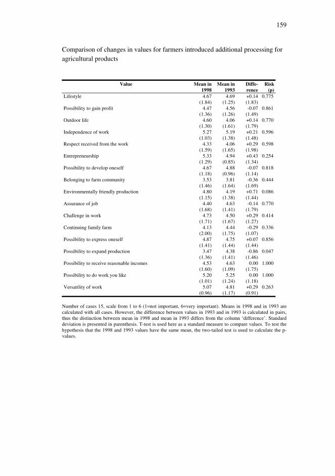
159

Comparison of changes in values for farmers introduced additional processing foragricultural products

Value Mean in1998

Mean in1993

Diffe-rence

Risk(p)

Lifestyle

Possibility to gain profit

Outdoor life

Independence of work

Respect received from the work

Entrepreneurship

Possibility to develop oneself

Belonging to farm community

Environmentally friendly production

Assurance of job

Challenge in work

Continuing family farm

Possibility to express oneself

Possibility to expand production

Possibility to receive reasonable incomes

Possibility to do work you like

Versatility of work

4.67(1.84)

4.47(1.36)

4.60(1.30)

5.27(1.03)

4.33(1.59)

5.33(1.29)

4.67(1.18)

3.53(1.46)

4.80(1.15)

4.40(1.68)

4.73(1.71)

4.13(2.00)

4.87(1.41)

3.47(1.36)

4.53(1.60)

5.20(1.01)

5.07(0.96)

4.69(1.25)

4.56(1.26)

4.06(1.61)

5.19(1.38)

4.06(1.65)

4.94(0.85)

4.88(0.96)

3.81(1.64)

4.19(1.38)

4.63(1.41)

4.50(1.67)

4.44(1.75)

4.75(1.44)

4.38(1.41)

4.63(1.09)

5.25(1.24)

4.81(1.17)

+0.14(1.83)-0.07

(1.49)+0.14(1.79)+0.21(1.48)+0.29(1.98)+0.43(1.34)-0.07

(1.14)-0.36

(1.69)+0.71(1.44)-0.14

(1.79)+0.29(1.27)-0.29

(1.07)+0.07(1.44)-0.86

(1.46)0.00

(1.75)0.00

(1.18)+0.29(0.91)

0.775

0.861

0.770

0.596

0.598

0.254

0.818

0.444

0.086

0.770

0.414

0.336

0.856

0.047

1.000

1.000

0.263

Number of cases 15, scale from 1 to 6 (1=not important, 6=very important). Means in 1998 and in 1993 arecalculated with all cases. However, the difference between values in 1993 and in 1993 is calculated in pairs,thus the distinction between mean in 1998 and mean in 1993 differs from the column ‘difference’. Standarddeviation is presented in parenthesis. T-test is used here as a standard measure to compare values. To test thehypothesis that the 1998 and 1993 values have the same mean, the two-tailed test is used to calculate the p-values.

160

Comparison of changes in values for farmers increased off-farm incomes

Value Mean in1998

Mean in1993

Diffe-rence

Risk(p)

Lifestyle

Possibility to gain profit

Outdoor life

Independence of work

Respect received from the work

Entrepreneurship

Possibility to develop oneself

Belonging to farm community

Environmentally friendly production

Assurance of job

Challenge in work

Continuing family farm

Possibility to express oneself

Possibility to expand production

Possibility to receive reasonable incomes

Possibility to do work you like

Versatility of work

4.89(1.44)

4.02(1.43)

4.55(1.34)

5.04(1.06)

3.72(1.65)

4.11(1,66)

3.89(1.49)

3.57(1.51)

4.25(1.25)

3.91(1.71)

4.02(1.56)

4.34(1.65)

4.26(1.44)

2.94(1.47)

4.19(1.51)

4.57(1.54)

4.59(1.39)

4.96(0.96)

4.17(1.44)

4.51(1.22)

5.26(1.06)

3.40(1.50)

4.55(1.30)

4.07(1.44)

3.47(1.45)

3.86(1.39)

3.89(1.70)

4.16(1.30)

4.47(1.53)

4.24(1.40)

3.35(1.49)

3.82(1.55)

4.76(1.36)

4.84(1.51)

-0.11(1.52)-0.15

(1.55)+0.02(1.26)-0.25

(1.22)+0.26(1.64)-0.47

(1.78)-0.25

(1.70)+0.08(1.54)+0.43(1.53)-0.02

(1.85)-0.21

(1.50)-0.17

(1.72)-0.04

(1.47)-0.42

(1.60)-0.32

(1.49)-0.23

(1.66)-0.28

(1.65)

0.589

0.478

0.914

0.150

0.247

0.060

0.298

0.723

0.043

0.941

0.318

0.475

0.852

0.064

0.123

0.325

0.216

Number of cases 53, scale from 1 to 6 (1=not important, 6=very important). Means in 1998 and in 1993 arecalculated with all cases. However, the difference between values in 1993 and in 1993 is calculated in pairs,thus the distinction between mean in 1998 and mean in 1993 differs from the column ‘difference’. Standarddeviation is presented in parenthesis. T-test is used here as a standard measure to compare values. To test thehypothesis that the 1998 and 1993 values have the same mean, the two-tailed test is used to calculate the p-values.