FARM WAGES AND LIVING STANDARDS IN THE INDUSTRIALREVOLUTION: ENGLAND, 1670-1850

Gregory ClarkDepartment of Economics

UC-Davis, Davis CA 95616gclark@ucdavis.edu

Using manuscript and secondary sources, this paper calculates a consistentseries of day wages for male farm workers in England from 1670 to 1850. Thenew series differs considerably for the years 1790-1820 from the still widelyused Bowley series. Wages are also estimated for four regions byquinquennia. The new series suggests that real agricultural wages showedlittle long term movement in the 180 years from 1670 to 1850. Real wages in1840-49 were only 20% above their level circa 1700. As expected real wagetrends differ sharply between the north and south. Real wages declined 10% inthe South West, but rose by 75% in the north. The flatness of the real wageseries implies Feinstein is too optimistic about real wages in general in theyears 1790-1820. It also is inconsistent with the claim of rapid productivityadvance in agriculture anytime in the years 1670-1850.

INTRODUCTION

Much has been written on agricultural wages in England from 1670 to 1850, but this

information has never been formed into one national series of agricultural wages. For the years

after 1770 Bowley calculated a wage index, mainly from secondary sources and wage surveys

for England and Wales that is still frequently quoted.1 Bowley’s index reports annual estimates

of wages from 1770 to 1914.2 But while his index is well founded in the years after 1824, for the

earlier period it relies on considerable interpolation, and takes no account of manuscript sources

that became available in the past 100 years. Elizabeth Gilboy derived from county bills

estimates of the wages of road workers in rural areas from 1700 to 1796, and these we can expect

1 See, for example, Feinstein (1995).

2

to approximate to agricultural wages.3 Bernard Eccleston in an unpublished Ph.D. thesis

calculated the day wages of workers on large agricultural estates from five midland counties

from 1750 to 1834, and gives an annual day wage series for these counties.4 Thomas Richardson

in another unpublished thesis similarly calculated the average wages in seven English counties

from 1790 to 1840 in part from estate sources.5 But while the Agrarian History of England and

Wales volume for 1750 to 1850 offers a number of wage series on individual farms, it gives no

overall wage series for the years 1750 to 1850.6

In the years before 1750 the information is much sparser. Peter Bowden calculated from

manuscript sources average winter day wages for some decades in six counties for the years

1640-1749. But he had no observations for the north of the country before 1690, and none for

the west of the country in any decade.7

The first task this paper thus undertakes is to produce a nominal national agricultural

wage index annually from 1670 to 1850 which incorporates the available published wage

information and manuscript sources. Manuscript observations contribute about two thirds of the

information at the annual level. I have also derived by quinquennia an index for each of four

major areas of the country for these years– the North, Midlands, South West and South East –

since these regions had very different wage trends in this period. I then consider what these

indices imply about the standard of living of agricultural workers.

The strategy followed throughout is to estimate a wage series from weekly wage

payments outside hay and harvest (44 out of 52 weeks in the year). I show that these “winter”

2 Bowley (1898), Bowley (1937)3 Gilboy (1934).4 Eccleston (1976).5 Richardson (1977).6 John (1989).7 Bowden (1985), p. 877-8.

3

wages are likely to represent annual wages by examining what happens to the ratio of hay wages

to winter wages and harvest wages to winter wages. I also check that the series is at

approximately the right level by comparing it with three “benchmark” cross sections of

agricultural wages. These are the 1834 Poor Law enquiry reports that collected wage

information by circulars in the winter of 1832-3, wages as reported in the Gardener’s Chronicle

and Agricultural Gazette in April 1850, and Arthur Young’s wage reports for 1767, 1768 and

1770.

Estimating Wages from Farm Accounts

There are three big problems with estimating wages from farm and estate accounts. The

first is knowing when the employee referred to is an adult male. Farms employed varying

numbers of women, boys, and girls for various tasks and paid them much less than adult males.

The accounts rarely show the age of workers, and often not even the gender. To make sure that

adult male wages only were included we can rely on the sexual division of labor which was

practiced in the English countryside from the middle ages on. Thus the tasks of threshing,

ditching, hedging, mowing, carting, cutting wood and making faggots, which together occupied a

large chunk of the agricultural year, seem to have been almost exclusively the jobs of adult male

workers. Farm tasks such as these can safely be included in the wage index. And once a worker

is identified as performing such tasks he can be safely presumed to be an adult male agricultural

laborer. Some tasks such as reaping and weeding were done by both men at women, at least in

earlier years, and these are only included where ancillary evidence shows the workers were adult

males. Again some tasks such as plowing often involved boys, and again are included only

where other evidence shows the worker was an adult male.

4

The second problem is knowing whether the worker received in addition to the wage

some of his pay as food, beer, cottage accommodation, an allotment, or the right to buy grain at

low prices. Such allowances are generally not recorded in these accounts. Detecting cases in

regular work where the worker was fed on the job is not so hard where farmers employed

workers both with and without food, since the wage with food would often be only a half or less

than the wage without food. Thus if we see two sets of wages at very different levels it is often

apparent that one is for wages with food.8 Detecting wages that included food at hay or harvest

time is very difficult since these wages could vary a great deal from regular wages, and food is a

smaller share of wages then. Fortunately in southern England at least provision of food to

workers was relatively rare by the late seventeenth century, and may have been unusual long

before that. In the north of England workers were often fed at work even in the nineteenth

century, and vigilance is required to avoid including such wages.

Detecting when workers in regular work received beer proves to be impossible from the

accounts, since beer was a much smaller supplement to wages, and so cannot be detected from

internal evidence. Beer was often still provided even in 1832, especially at hay and harvest. But

the evidence from the 1834 Poor Law report is that where beer was provided it was worth about

10% of wages in winter and summer, and less than this in harvest. Thus changes in the degree of

beer provision will have some effect on wages, but not too dramatic an effect.

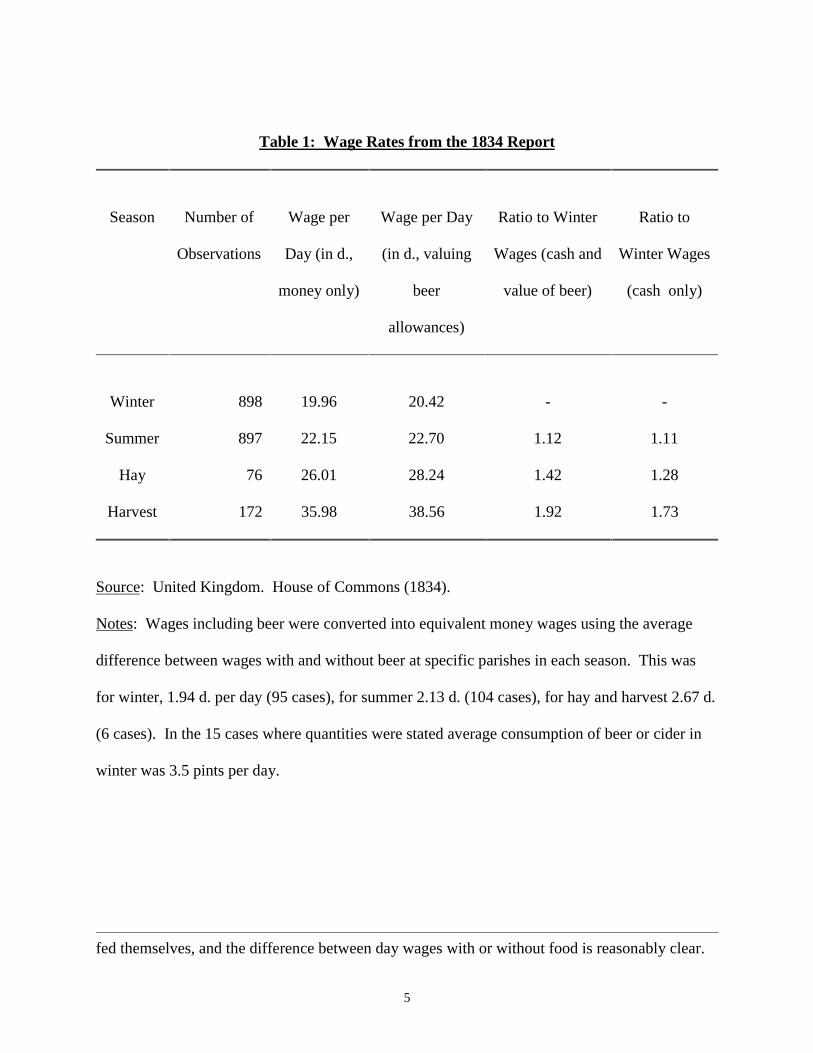
The third problem is that wages varied over the course of the year, being lowest in the

midwinter, and highest at the grain harvest. Table 1 shows for the 1832 wages in the Poor Law

report the level of wages in winter, summer, hay time, and harvest. Money wages at harvest

were nearly twice the level of wages in winter.

8 See, for example, Harland (1856), which records wages on the Shuttleworth estate inLancashire. Workers on the home farm were generally fed, but workers at outlying tithe barns

5

Table 1: Wage Rates from the 1834 Report

Season Number of

Observations

Wage per

Day (in d.,

money only)

Wage per Day

(in d., valuing

beer

allowances)

Ratio to Winter

Wages (cash and

value of beer)

Ratio to

Winter Wages

(cash only)

Winter 898 19.96 20.42 - -

Summer 897 22.15 22.70 1.12 1.11

Hay 76 26.01 28.24 1.42 1.28

Harvest 172 35.98 38.56 1.92 1.73

Source: United Kingdom. House of Commons (1834).

Notes: Wages including beer were converted into equivalent money wages using the average

difference between wages with and without beer at specific parishes in each season. This was

for winter, 1.94 d. per day (95 cases), for summer 2.13 d. (104 cases), for hay and harvest 2.67 d.

(6 cases). In the 15 cases where quantities were stated average consumption of beer or cider in

winter was 3.5 pints per day.

fed themselves, and the difference between day wages with or without food is reasonably clear.

6

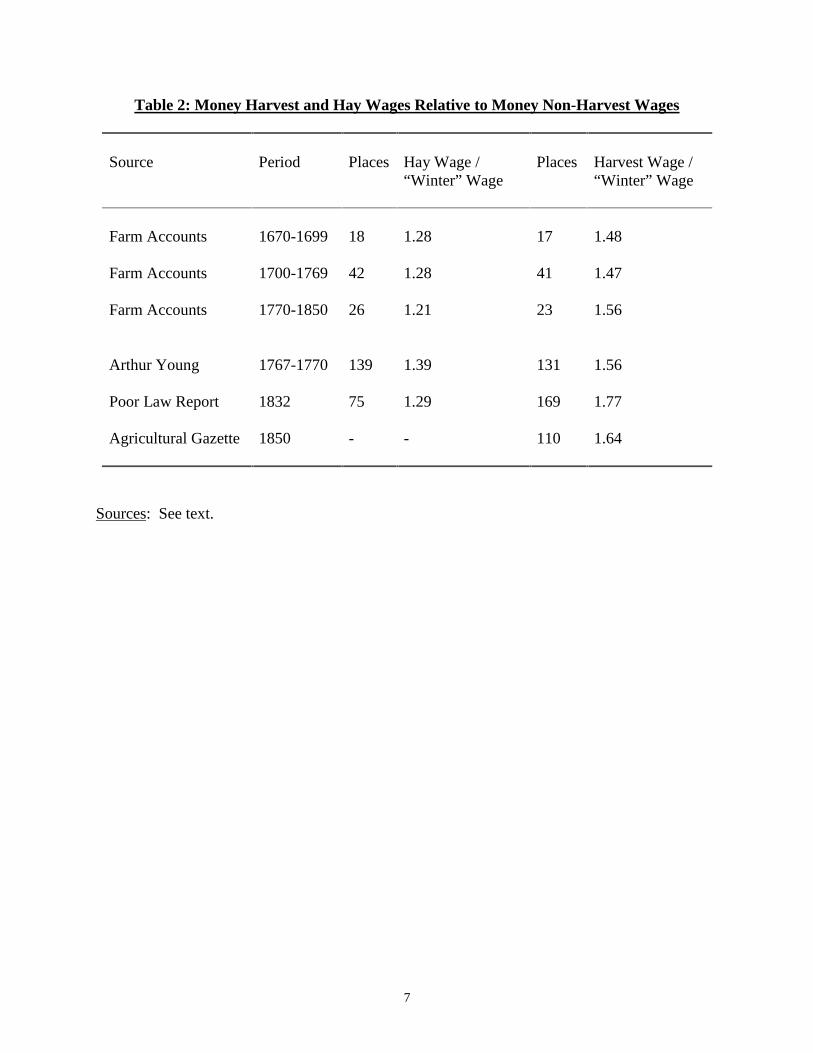
To deal with this last problem I first note that the ratio of harvest and hay wages to winter

and summer wages changed little over time. Table 2 shows the ratio of money wage payments at

harvest and hay to non-harvest wages from the farm accounts used in the wage index from 1670

on. As can be seen the ratio does not change much over the course of 180 years, and most of the

apparent change may just be sampling error. The ratios in the farm accounts are also relatively

similar to the various benchmark cross sections that we have from 1770, 1832, and 1850. This

implies that as long as I have a geographically representative sample of places I can use the

winter and summer day wages as a good index of annual earnings at least back as far as 1670,

assuming full employment of workers.

If we take harvest wages at being at the level suggested in Table 1 for 1832, for example,

then the earnings of the a worker who worked 52 weeks in the year in 1832 would be £30.4.

Earnings outside harvest and hay would thus be 77% of total earnings. Hence the modest

changes in the ratio of hay and harvest wages to winter wages observed in Table 2 would change

total annual earnings for a fully employed worker by only 1 or 2%. For example, the 1834 report

suggests harvest wages were 1.92 times winter wages (counting beer and food allowances).

Suppose before 1770 they were only 1.68imes winter wages as table 2 would imply. In that case

annual earnings would be 1.9% less than would be suggested by an index based only on winter

wages. Thus a wage series based on non-harvest wages will in general present a pretty good

picture of wage trends.

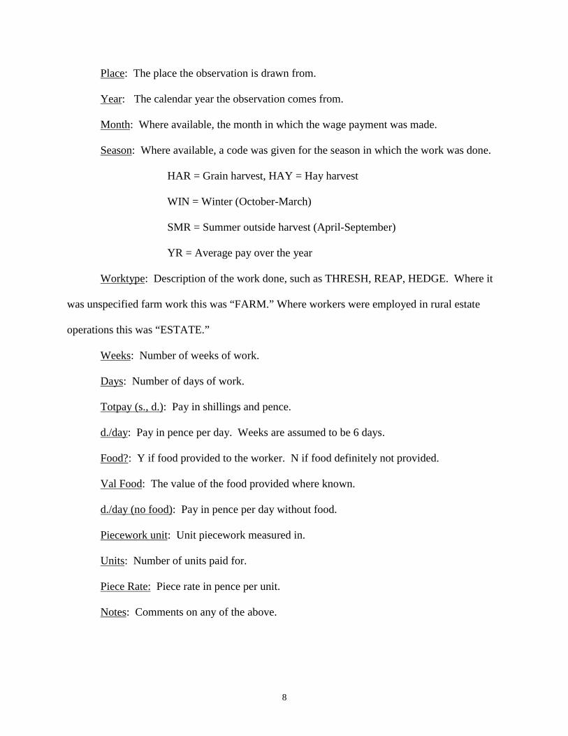
The various sources of wage information used have been combined into an “Agricultural

Wages” data set that records the following information where available:

7

Table 2: Money Harvest and Hay Wages Relative to Money Non-Harvest Wages

Source Period Places Hay Wage /“Winter” Wage

Places Harvest Wage /“Winter” Wage

Farm Accounts 1670-1699 18 1.28 17 1.48

Farm Accounts 1700-1769 42 1.28 41 1.47

Farm Accounts 1770-1850 26 1.21 23 1.56

Arthur Young 1767-1770 139 1.39 131 1.56

Poor Law Report 1832 75 1.29 169 1.77

Agricultural Gazette 1850 - - 110 1.64

Sources: See text.

8

Place: The place the observation is drawn from.

Year: The calendar year the observation comes from.

Month: Where available, the month in which the wage payment was made.

Season: Where available, a code was given for the season in which the work was done.

HAR = Grain harvest, HAY = Hay harvest

WIN = Winter (October-March)

SMR = Summer outside harvest (April-September)

YR = Average pay over the year

Worktype: Description of the work done, such as THRESH, REAP, HEDGE. Where it

was unspecified farm work this was “FARM.” Where workers were employed in rural estate

operations this was “ESTATE.”

Weeks: Number of weeks of work.

Days: Number of days of work.

Totpay (s., d.): Pay in shillings and pence.

d./day: Pay in pence per day. Weeks are assumed to be 6 days.

Food?: Y if food provided to the worker. N if food definitely not provided.

Val Food: The value of the food provided where known.

d./day (no food): Pay in pence per day without food.

Piecework unit: Unit piecework measured in.

Units: Number of units paid for.

Piece Rate: Piece rate in pence per unit.

Notes: Comments on any of the above.

9

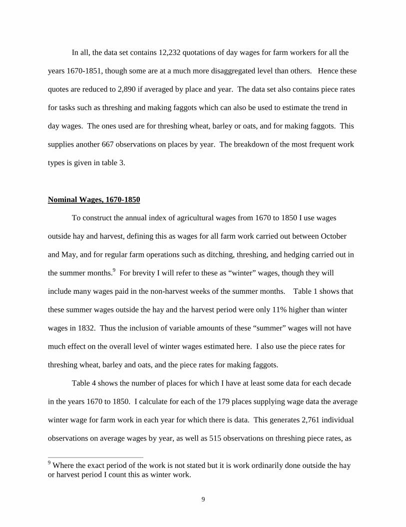
In all, the data set contains 12,232 quotations of day wages for farm workers for all the

years 1670-1851, though some are at a much more disaggregated level than others. Hence these

quotes are reduced to 2,890 if averaged by place and year. The data set also contains piece rates

for tasks such as threshing and making faggots which can also be used to estimate the trend in

day wages. The ones used are for threshing wheat, barley or oats, and for making faggots. This

supplies another 667 observations on places by year. The breakdown of the most frequent work

types is given in table 3.

Nominal Wages, 1670-1850

To construct the annual index of agricultural wages from 1670 to 1850 I use wages

outside hay and harvest, defining this as wages for all farm work carried out between October

and May, and for regular farm operations such as ditching, threshing, and hedging carried out in

the summer months.9 For brevity I will refer to these as “winter” wages, though they will

include many wages paid in the non-harvest weeks of the summer months. Table 1 shows that

these summer wages outside the hay and the harvest period were only 11% higher than winter

wages in 1832. Thus the inclusion of variable amounts of these “summer” wages will not have

much effect on the overall level of winter wages estimated here. I also use the piece rates for

threshing wheat, barley and oats, and the piece rates for making faggots.

Table 4 shows the number of places for which I have at least some data for each decade

in the years 1670 to 1850. I calculate for each of the 179 places supplying wage data the average

winter wage for farm work in each year for which there is data. This generates 2,761 individual

observations on average wages by year, as well as 515 observations on threshing piece rates, as

9 Where the exact period of the work is not stated but it is work ordinarily done outside the hayor harvest period I count this as winter work.

10

Table 3: Amounts of Data in the Wage Data Set

Work type Individual observations Observations averaged byyear and place

DAY WAGESAll 12,232 2,890“Farm” 7,341 1,645Hedge 882 391“Estate” (Eccleston) 513 513Thresh and winnow 475 218Mow .. 453 330Labor in Garden 334 184Cart 222 79“harvest” 217 194Ditch 186 132Plow 182 71“Dung” 175 95“Labor” 153 136Dig 143 103Reap 125 100

PIECE RATESThreshing wheat, barley oroats

2,911 515

Making faggots 232 142

Source: Agricultural Wage Data Set.

11

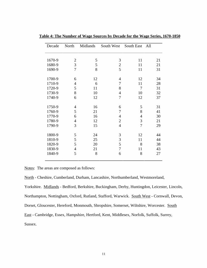
Table 4: The Number of Wage Sources by Decade for the Wage Series, 1670-1850

Decade North Midlands South West South East All

1670-9 2 5 3 11 211680-9 3 5 2 11 211690-9 7 8 5 11 31

1700-9 6 12 4 12 341710-9 4 6 7 11 281720-9 5 11 8 7 311730-9 8 10 4 10 321740-9 6 12 7 12 37

1750-9 4 16 6 5 311760-9 5 21 7 8 411770-9 6 16 4 4 301780-9 4 12 2 3 211790-9 3 15 4 7 29

1800-9 5 24 3 12 441810-9 5 25 3 11 441820-9 5 20 5 8 381830-9 4 21 7 11 431840-9 5 8 6 8 27

Notes: The areas are composed as follows:

North - Cheshire, Cumberland, Durham, Lancashire, Northumberland, Westmoreland,

Yorkshire. Midlands - Bedford, Berkshire, Buckingham, Derby, Huntingdon, Leicester, Lincoln,

Northampton, Nottingham, Oxford, Rutland, Stafford, Warwick. South West - Cornwall, Devon,

Dorset, Gloucester, Hereford, Monmouth, Shropshire, Somerset, Wiltshire, Worcester. South

East - Cambridge, Essex, Hampshire, Hertford, Kent, Middlesex, Norfolk, Suffolk, Surrey,

Sussex.

12

well as 142 observations on rates paid for making faggots.10 The data has been divided up into

these four regions because of indications that wages moved in different ways in each of these

regions in this period. Thus the north went from the lowest wage to the highest wage region over

this period. And the South East went from being about 20% above the national average wage

level to being 10% below the national average. As can be seen there is much more data for some

regions than for others, and the relative amount of information varies by period.

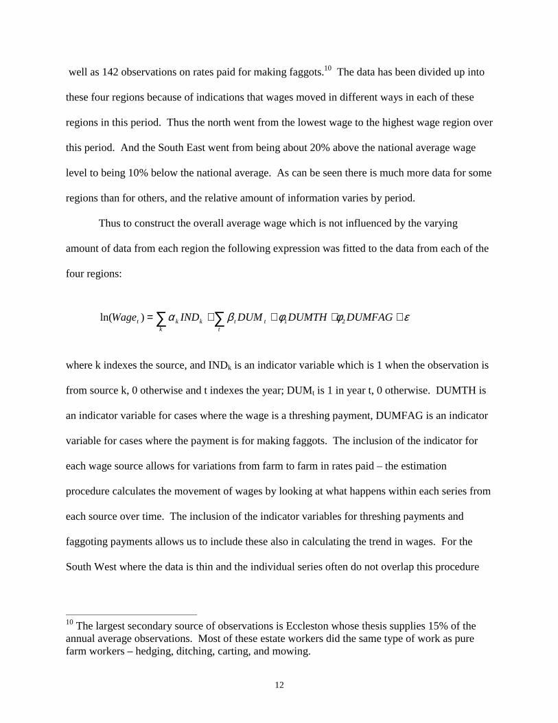
Thus to construct the overall average wage which is not influenced by the varying

amount of data from each region the following expression was fitted to the data from each of the

four regions:

where k indexes the source, and INDk is an indicator variable which is 1 when the observation is

from source k, 0 otherwise and t indexes the year; DUMt is 1 in year t, 0 otherwise. DUMTH is

an indicator variable for cases where the wage is a threshing payment, DUMFAG is an indicator

variable for cases where the payment is for making faggots. The inclusion of the indicator for

each wage source allows for variations from farm to farm in rates paid – the estimation

procedure calculates the movement of wages by looking at what happens within each series from

each source over time. The inclusion of the indicator variables for threshing payments and

faggoting payments allows us to include these also in calculating the trend in wages. For the

South West where the data is thin and the individual series often do not overlap this procedure

10 The largest secondary source of observations is Eccleston whose thesis supplies 15% of theannual average observations. Most of these estate workers did the same type of work as purefarm workers – hedging, ditching, carting, and mowing.

εφφβα ++++= ∑∑ DUMFAGDUMTHDUMINDWaget

ttk

kkt 21)ln(

13

did not work well, and the indicator variables for each source were not used (in effect I had to

assume that the average wage level at any time was the same across sources in the South West).

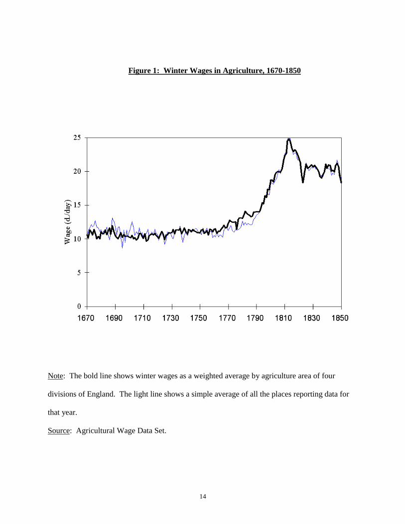
The national wage is calculated as the weighted average of the estimated wage in each

region, weighting by the numbers of male agricultural workers in each region recorded in the

1851 census.11 Figure 1 shows as the faint line the raw average winter day wage in each year.

The bold line is the wage index calculated from the above regression for each region, and

averaged across each region. As can be seen the corrected index differs little from the

uncorrected index in most years. In the years 1670-1720 it is generally below the raw average,

while in 1760-1790 it is generally above the raw average. Nominal agricultural wages are

essentially flat in the years 1670 to 1730, at an average rate of about 10.3 d. per day in the

winter. Thereafter there is a rise to a peak in 1813, followed by a decline to the 1820s. With the

exception of notable downturns in 1822-4, and 1834-37, and 1848-50 wages are fairly steady

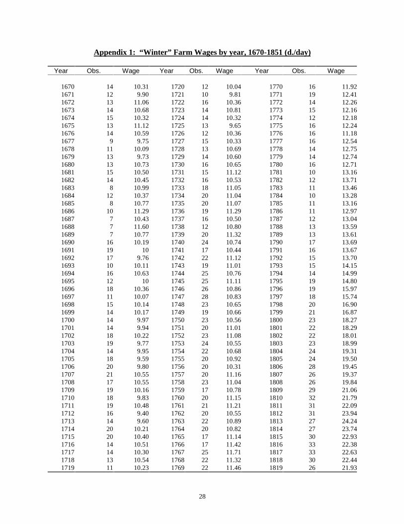
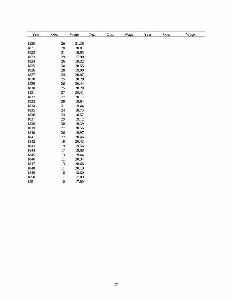
between 1820 and 1850. Appendix 1 shows annual estimated nominal day wages from 1670 to

1850.

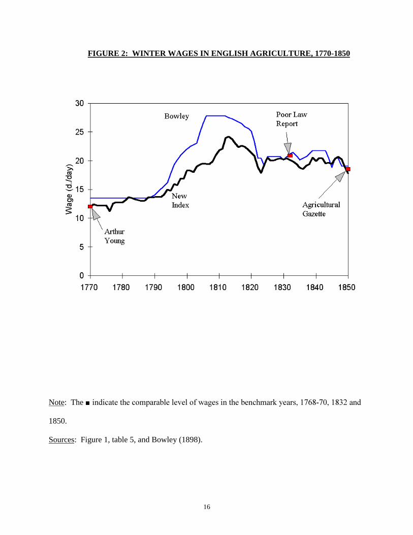
Figure 2 compares this series with the Bowley index. The Bowley index was constructed

using a few cross sections of wages – 1770, 1796, 1824, 1832, 1837, 1850 - interpolated using

records for a small number of farms. For the years after 1820 the two series move closely

together. But for some of the earlier dates, and in particular 1795-1820 the Bowley series is

very different. Thus in 1807 Bowley reports wages at 27.8 d. per day, while the new series

11I counted all farm workers between the ages of 15 and 65, including farmers, in thiscalculation. The numbers were respectively North, 240,124, Midlands, 284,676, South East,334,163, South West, 278,001.

14

Figure 1: Winter Wages in Agriculture, 1670-1850

Note: The bold line shows winter wages as a weighted average by agriculture area of four

divisions of England. The light line shows a simple average of all the places reporting data for

that year.

Source: Agricultural Wage Data Set.

15

reports only 19.4 d., a 44% difference. Bowley is generally much more optimistic about the

level of rural wages for the Revolutionary and Napoleonic war period.12

Feinstein uses the Bowley series for agricultural wages in his recent article on real wages

in Britain in the Industrial Revolution period, and agricultural workers were almost a third of the

labor force in the early Industrial Revolution. These wage estimates suggest that Feinstein will

have overestimated real wages in the years 1800-1820 when the Bowley series overstates

nominal agricultural wages very substantially.

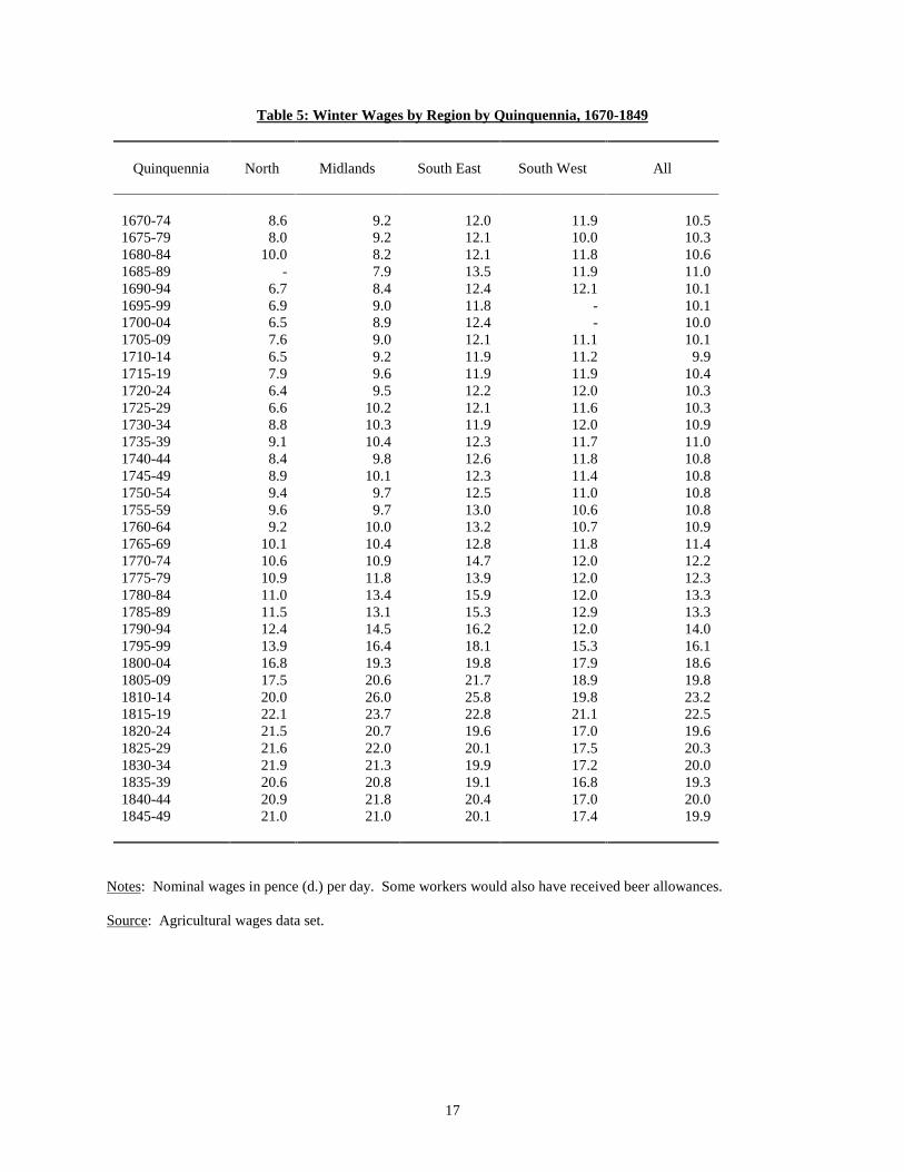
Table 5 shows by quinquennia the estimated movement of wages in each of the four

regions. As can be seen both the North and the Midlands move from having wages 20% below

the national average in the years 1670-1699 to having wages nearly 5% above the national

average in the 1840s. The South East in contrast moves from being about 20% above the

national average to being at the national average by 1845. And the South West moves from

being nearly 20% above the national average to being nearly 10% below by the 1840s.

12 This seems to be because Bowley’s interpolation was based on a small group of farms in thesouth east. We shall see below that wages peaked much more in the years 1800-1820 in theSouth East and the Midlands than in the North and South West.

16

FIGURE 2: WINTER WAGES IN ENGLISH AGRICULTURE, 1770-1850

Note: The �LQGLFDWH�WKH�FRPSDUDEOH�OHYHO�RI�ZDJHV�LQ�WKH�EHQFKPDUN�\HDUV����������������DQG

1850.

Sources: Figure 1, table 5, and Bowley (1898).

17

Table 5: Winter Wages by Region by Quinquennia, 1670-1849

Quinquennia North Midlands South East South West All

1670-74 8.6 9.2 12.0 11.9 10.51675-79 8.0 9.2 12.1 10.0 10.31680-84 10.0 8.2 12.1 11.8 10.61685-89 - 7.9 13.5 11.9 11.01690-94 6.7 8.4 12.4 12.1 10.11695-99 6.9 9.0 11.8 - 10.11700-04 6.5 8.9 12.4 - 10.01705-09 7.6 9.0 12.1 11.1 10.11710-14 6.5 9.2 11.9 11.2 9.91715-19 7.9 9.6 11.9 11.9 10.41720-24 6.4 9.5 12.2 12.0 10.31725-29 6.6 10.2 12.1 11.6 10.31730-34 8.8 10.3 11.9 12.0 10.91735-39 9.1 10.4 12.3 11.7 11.01740-44 8.4 9.8 12.6 11.8 10.81745-49 8.9 10.1 12.3 11.4 10.81750-54 9.4 9.7 12.5 11.0 10.81755-59 9.6 9.7 13.0 10.6 10.81760-64 9.2 10.0 13.2 10.7 10.91765-69 10.1 10.4 12.8 11.8 11.41770-74 10.6 10.9 14.7 12.0 12.21775-79 10.9 11.8 13.9 12.0 12.31780-84 11.0 13.4 15.9 12.0 13.31785-89 11.5 13.1 15.3 12.9 13.31790-94 12.4 14.5 16.2 12.0 14.01795-99 13.9 16.4 18.1 15.3 16.11800-04 16.8 19.3 19.8 17.9 18.61805-09 17.5 20.6 21.7 18.9 19.81810-14 20.0 26.0 25.8 19.8 23.21815-19 22.1 23.7 22.8 21.1 22.51820-24 21.5 20.7 19.6 17.0 19.61825-29 21.6 22.0 20.1 17.5 20.31830-34 21.9 21.3 19.9 17.2 20.01835-39 20.6 20.8 19.1 16.8 19.31840-44 20.9 21.8 20.4 17.0 20.01845-49 21.0 21.0 20.1 17.4 19.9

Notes: Nominal wages in pence (d.) per day. Some workers would also have received beer allowances.

Source: Agricultural wages data set.

18

The New Series Compared to Benchmark Estimates of Wages

How good an indication is this series, constructed on the basis of an average of 19

randomly located places per year, of the movement of wages? The answer, at least for the years

after 1768, seems to be that it is likely to be pretty accurate at the national level. I measure how

well the new series is likely to represent wage trends by comparing its average level to average

wages nationally in three years where we have extensive data from across the country: 1767-70,

1832 and 1850. The 1832 benchmark is the best of all, since it comes from a large sample of

parishes. Calculating wages the same way as is used in the index, I get the national and regional

wages in 1832 from the Poor Law reports as shown in Table 5, based on 908 day wage

observations. The Poor Law reports suggest an average money wage outside harvest and hay of

20.9 d. per day.13 The wage index estimates national wages in the same year as 20.2 d., an error

of less than 4% if we take the poor law reports as definitive. For 1767-70 Arthur Young gives

160 day wages, which imply an average money wage of 12.0 d., versus the wage index which

shows 11.6 d, for a difference of again less than 4%. For 1850 the Agricultural Gazette reports

127 wages for April of 1850 in 38 of 42 counties in England, which suggest a national average

wage of 18.5 d., versus my index which is then at 17.8 d., again a difference of only 4%. Thus

on a national scale we can seemingly expect that the wage index will show wages within about

4% of their true national level in the years 1670 to 1850, since the number of farms observed in

each ten year period is about the same throughout.

As expected the regional wage levels deviate more from their respective benchmarks.

But only in two cases does the deviation exceed 10% in any of the benchmark years. The

regional indices can thus

13 To calculate this wage I assume winter wages covered six of the ten months outside harvest,and summer wages the other four.

19

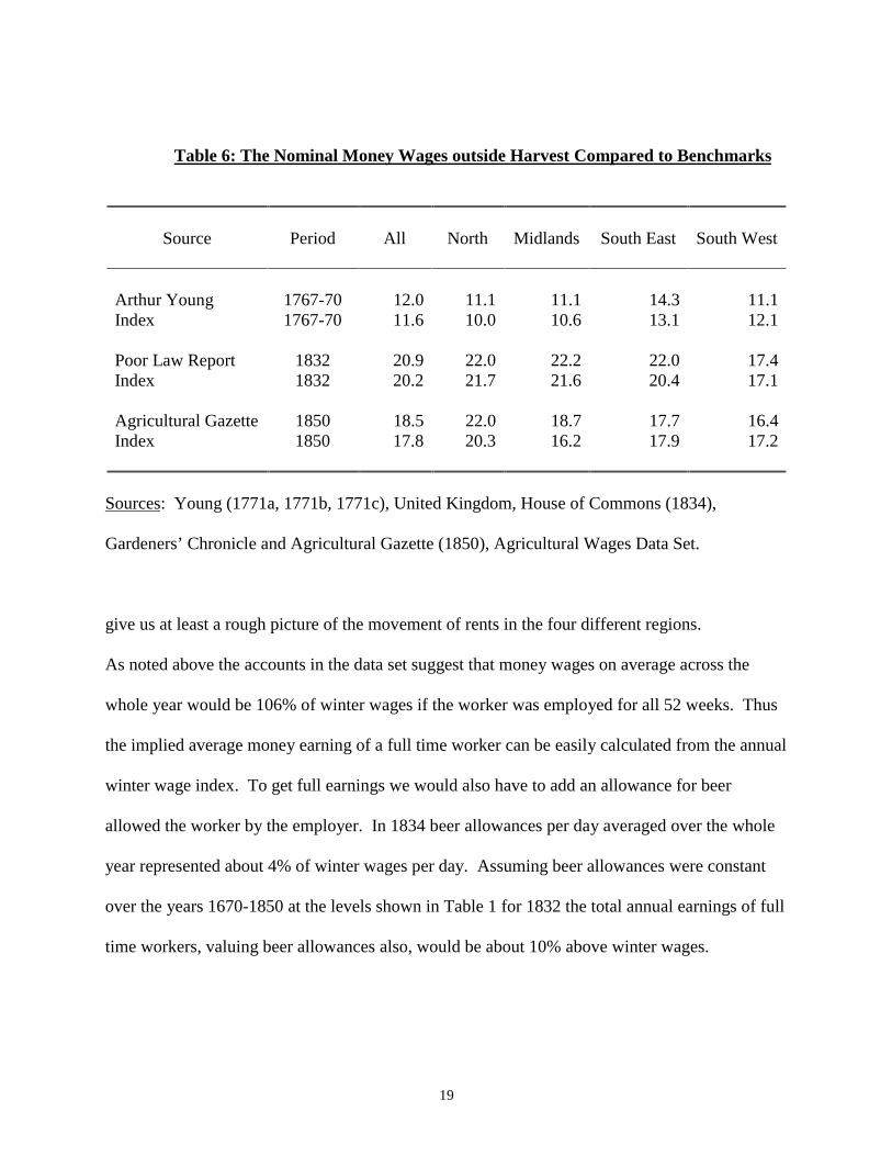
Table 6: The Nominal Money Wages outside Harvest Compared to Benchmarks

Source Period All North Midlands South East South West

Arthur Young 1767-70 12.0 11.1 11.1 14.3 11.1Index 1767-70 11.6 10.0 10.6 13.1 12.1

Poor Law Report 1832 20.9 22.0 22.2 22.0 17.4Index 1832 20.2 21.7 21.6 20.4 17.1

Agricultural Gazette 1850 18.5 22.0 18.7 17.7 16.4Index 1850 17.8 20.3 16.2 17.9 17.2

Sources: Young (1771a, 1771b, 1771c), United Kingdom, House of Commons (1834),

Gardeners’ Chronicle and Agricultural Gazette (1850), Agricultural Wages Data Set.

give us at least a rough picture of the movement of rents in the four different regions.

As noted above the accounts in the data set suggest that money wages on average across the

whole year would be 106% of winter wages if the worker was employed for all 52 weeks. Thus

the implied average money earning of a full time worker can be easily calculated from the annual

winter wage index. To get full earnings we would also have to add an allowance for beer

allowed the worker by the employer. In 1834 beer allowances per day averaged over the whole

year represented about 4% of winter wages per day. Assuming beer allowances were constant

over the years 1670-1850 at the levels shown in Table 1 for 1832 the total annual earnings of full

time workers, valuing beer allowances also, would be about 10% above winter wages.

20

The Purchasing Power of Farm Wages

Having now generated a nominal wage series for agricultural laborers, we can also ask

what happened to the real purchasing power of wages in this interval. To measure this I use the

weights for expenditures by rural families given in the last column of table 10. These weights,

with the exception of that for housing, are derived from data given by Sara Horrell for the

expenditures of agricultural workers in 1787-96, 1830-39 and 1840-54 and shown in the first two

columns.14 Since I have better data on housing costs than these surveys will reveal, I estimated

housing expenditures directly. In 1832 the average male agricultural worker would earn in a full

year an annual income of £29.1, including the implied value of beer allowances at work. The

other members of the family together are assumed to earn 25% of the adult male’s wage.15 Thus

the average family would have an income of £36.4 per year. Average cottage rents on a set of

1,206 cottages owned by charities in England in the years 1830 to 1837, adjusted to control for

oversampling in more densely populated parishes were £3.25.16 This implies that in the early

1830s cottage rents were 8.9% of family incomes for agricultural workers, close to the 8.8% that

Horrell found for 1830-54.

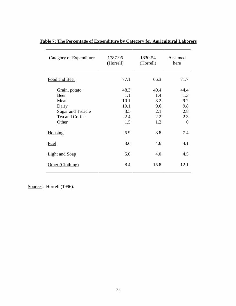
The quinquennia price levels for the major commodity groups used to form the cost of

living index are shown in table 11. For bread, the staple article which formed nearly half of farm

laborers expenditures, I use the prices of wheat, barley and oats. Even though these were only

the inputs into making bread, I use these because bread had very different qualities which are

very hard to control for over long time intervals, and because the cost of the inputs was a very

large share of the cost of outputs for bread.

14 Horrell (1996), pp. 568-70.15 Based on Clark (1991), p. 254.16 The source of this housing rental information is discussed in Clark (1998).

21

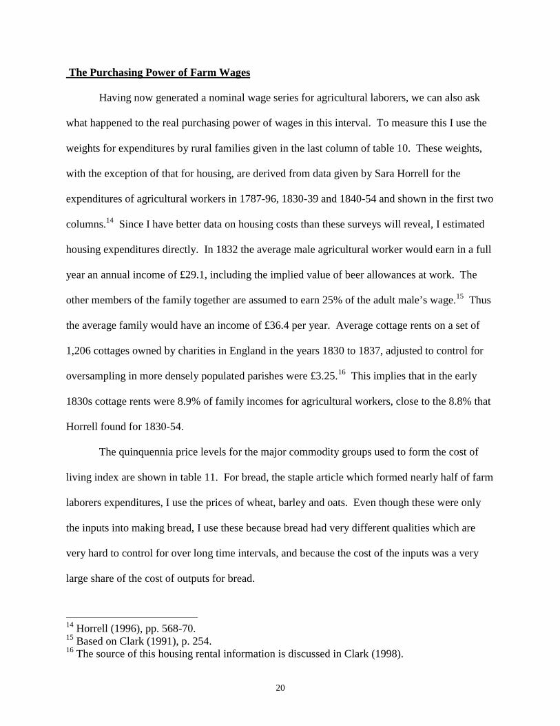
Table 7: The Percentage of Expenditure by Category for Agricultural Laborers

Category of Expenditure 1787-96(Horrell)

1830-54(Horrell)

Assumedhere

Food and Beer 77.1 66.3 71.7

Grain, potato 48.3 40.4 44.4 Beer 1.1 1.4 1.3 Meat 10.1 8.2 9.2 Dairy 10.1 9.6 9.8 Sugar and Treacle 3.5 2.1 2.8 Tea and Coffee 2.4 2.2 2.3 Other 1.5 1.2 0

Housing 5.9 8.8 7.4

Fuel 3.6 4.6 4.1

Light and Soap 5.0 4.0 4.5

Other (Clothing) 8.4 15.8 12.1

Sources: Horrell (1996).

22

Table 8: Index of Farm Laborers’ Living Costs, 1670-1850

Quin. Grain Beer Meat Dairy Sugar Tea Fuel Candlesand soap

Rent Clothing Cost ofLiving

1670-74 73 74 73 94 83 90 94 79.91675-79 77 74 68 122 94 87 90 100 82.11680-84 73 73 64 122 93 76 90 97 78.61685-89 66 73 68 107 93 75 90 94 74.91690-94 73 73 74 122 92 83 90 94 79.61695-99 91 80 79 159 92 89 90 108 92.81700-04 68 77 74 69 120 88 81 76 106 76.51705-09 68 77 69 63 122 88 74 76 107 74.91710-14 88 79 75 72 116 84 88 76 109 87.01715-19 71 80 73 61 110 84 90 76 108 77.31720-24 72 80 72 64 102 84 82 79 109 77.51725-29 87 82 73 68 102 84 82 79 109 85.71730-34 64 85 71 67 93 87 76 79 104 72.81735-39 72 85 66 64 92 87 68 79 104 76.11740-44 75 85 76 73 100 88 92 100 104 82.41745-49 63 85 72 64 114 88 89 100 106 74.61750-54 70 86 71 89 114 88 84 100 103 80.61755-59 86 85 78 85 112 88 89 100 104 89.71760-64 69 85 76 81 100 100 87 100 111 103 80.91765-69 94 85 91 86 92 100 87 101 111 99 94.71770-74 100 100 100 100 100 100 100 100 100 100 100.01775-79 89 106 99 102 106 100 105 98 100 100 95.31780-84 96 118 96 94 120 100 90 103 99 100 97.61785-89 95 127 107 102 104 75 88 106 99 93 96.91790-94 108 132 111 115 141 69 94 100 106 99 106.61795-99 132 135 142 135 168 73 102 110 106 105 124.31800-04 172 156 191 157 111 90 114 141 98 112 148.41805-09 172 174 186 180 99 111 124 146 137 120 156.41810-14 204 173 216 201 137 109 126 166 193 122 180.71815-19 167 166 177 175 120 99 114 141 164 127 155.71820-24 120 152 156 145 85 86 110 98 164 122 124.91825-29 136 155 166 160 78 78 107 89 176 119 133.41830-34 123 133 140 148 63 73 83 98 185 124 123.51835-39 124 126 131 155 88 59 90 182 124.8*1840-44 122 107 132 155 93 62 82 127.5*1845-49 122 127 140 156 68 48 72 131.3*1850-54 109 134 137 143 58 50 74

Notes: The index for each commodity and overall is set to 100 for 1770-4. Feinstein’s overall

cost of living index was used for the years 1835-49. The commodities and the weights used for

each category of good where more than one was used were: Grain - wheat, 1670-1850 (.5),

23

barley, 1670-1850 (.3), oats, 1670-1850 (.2); Meat - beef, 1670-1850 (.5), mutton, 1670-1850

(.5); Dairy - Cheese, 1670-1850 (.5), butter, 1670-1850 (.5); Fuel - faggots, 1670-1830 (.5), coal

1770-1850 (.5); Light and Soap - Tallow candles 1670-1830 (.5), Tallow 1670-1830 (.5);

Cottage Rents - Charity owned cottages outside major cities, 1670-1837; Clothing - wool cloth,

1670-1829 (.5), linen cloth 1670-1829 (.2), stockings 1710-1830 (.1), shoes 1670-1830 (.2);

Sources: Thorold Rogers (1888), pp. 209-218, 255-277, 282-96, 474-94. Bowden (1985), pp.

828-31, 843-6. Beveridge (1939), pp. 85-90, 143-8, 193-6, 236-240, 292-5, 313, 434-7, 457-8.

John (1989). Feinstein (1998), p. 640.

24

For fuel I use the price of faggots only until 1770 since in rural areas these were the main

source of fuel until the nineteenth century at least. From 1770-1830 I use a combination of the

prices of faggots and coal, and after 1830 coal alone.17 For light and soap I use the prices of

tallow candles and of tallow, the main input in making soap, from 1670 to 1830. Cottage rents

are estimated from the rents and prices of cottage properties in rural areas (defined as parishes

with a population density of less than 1 person per acre in 1841) bought or owned by charities.

The details of this estimation are given in the appendix.

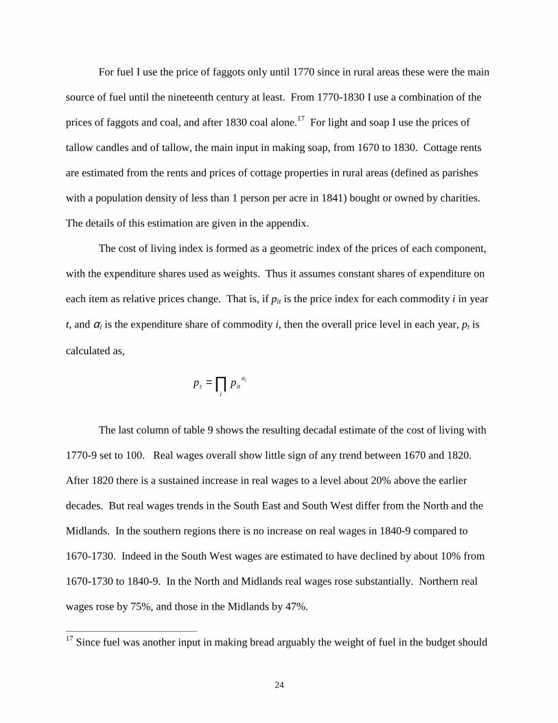
The cost of living index is formed as a geometric index of the prices of each component,

with the expenditure shares used as weights. Thus it assumes constant shares of expenditure on

each item as relative prices change. That is, if pit is the price index for each commodity i in year

t, and αi is the expenditure share of commodity i, then the overall price level in each year, pt is

calculated as,

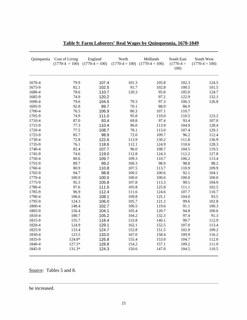
The last column of table 9 shows the resulting decadal estimate of the cost of living with

1770-9 set to 100. Real wages overall show little sign of any trend between 1670 and 1820.

After 1820 there is a sustained increase in real wages to a level about 20% above the earlier

decades. But real wages trends in the South East and South West differ from the North and the

Midlands. In the southern regions there is no increase on real wages in 1840-9 compared to

1670-1730. Indeed in the South West wages are estimated to have declined by about 10% from

1670-1730 to 1840-9. In the North and Midlands real wages rose substantially. Northern real

wages rose by 75%, and those in the Midlands by 47%.

17 Since fuel was another input in making bread arguably the weight of fuel in the budget should

∏=i

aitt

ipp

25

Table 9: Farm Laborers’ Real Wages by Quinquennia, 1670-1849

Quinquenia Cost of Living(1770-4 = 100)

England(1770-4 = 100)

North (1770-4 = 100)

Midlands(1770-4 = 100)

South East(1770-4 =

100)

South West(1770-4 = 100)

1670-4 79.9 107.4 101.3 105.8 102.3 124.51675-9 82.1 102.5 91.7 102.8 100.5 101.51680-4 78.6 110.7 120.3 95.8 105.0 124.71685-9 74.9 120.2 97.2 122.9 132.11690-4 79.6 104.5 79.3 97.3 106.3 126.81695-9 92.8 89.7 70.1 88.9 86.91700-4 76.5 106.9 80.3 107.1 110.71705-9 74.9 111.0 95.8 110.0 110.5 123.21710-4 87.0 93.4 69.8 97.4 93.4 107.01715-9 77.3 110.4 96.0 113.9 104.9 128.41720-4 77.5 108.7 78.1 113.0 107.4 129.11725-9 85.7 98.9 72.0 109.7 96.2 112.41730-4 72.8 122.6 113.9 130.2 111.8 136.91735-9 76.1 118.6 112.1 124.9 110.6 128.31740-4 82.4 107.7 96.0 108.7 104.5 119.51745-9 74.6 119.0 112.8 124.3 112.2 127.81750-4 80.6 109.7 109.3 110.7 106.2 113.41755-9 89.7 99.2 100.3 98.9 98.8 98.21760-4 80.9 110.8 107.5 113.7 110.9 109.91765-9 94.7 98.8 100.5 100.6 92.1 104.11770-4 100.0 100.0 100.0 100.0 100.0 100.01775-9 95.3 105.8 107.8 113.3 99.5 104.91780-4 97.6 111.5 105.8 125.8 111.1 102.51785-9 96.9 112.4 111.6 124.6 107.7 110.71790-4 106.6 108.1 109.8 125.1 104.0 93.51795-9 124.3 106.0 105.7 121.2 99.6 102.81800-4 148.4 102.7 106.5 119.6 91.1 100.31805-9 156.4 104.1 105.4 120.7 94.8 100.61810-4 180.7 105.2 104.2 132.3 97.4 91.31815-9 155.7 118.4 133.8 140.1 99.7 112.91820-4 124.9 129.1 162.1 152.5 107.0 113.41825-9 133.4 124.7 152.8 151.5 102.9 109.21830-4 123.5 133.0 167.0 158.4 109.9 116.21835-9 124.8* 126.8 155.4 153.0 104.7 112.01840-4 127.5* 128.8 154.2 157.1 109.2 111.01845-9 131.3* 124.3 150.6 147.0 104.5 110.5

Source: Tables 5 and 8.

be increased.

26

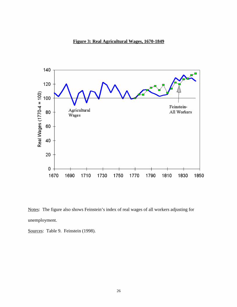
Figure 3: Real Agricultural Wages, 1670-1849

Notes: The figure also shows Feinstein’s index of real wages of all workers adjusting for

unemployment.

Sources: Table 9. Feinstein (1998).

27

The real wages given in table 9 are for a day’s work by male agricultural workers. The

movement of real family incomes will not be the same as real day wages if the number of work

days per year per worker changes because of involuntary unemployment, or if the incomes

earned by women and children change because of shifts in the nature of labor demand. Clark

and van der Werf (1998) considers the issue of the length of the work year for male workers in

greater depth.

Conclusion

The real wage of male farm workers, measured as the purchasing power of the day wage,

increased little if at all in the Industrial Revolution. Indeed workers in the southern regions may

have seen declines in their real wages. These findings are in line with Feinstein’s recent

pessimism about real wages in general in the Industrial Revolution. Indeed the agricultural wage

series developed here suggests that the Bowley series of agricultural wages used by Feinstein

may greatly overstate farm wages in the years 1790-1820. Feinstein’s pessimistic estimates are

still too optimistic in the Revolutionary and Napoleonic War years!

The flatness of the farm real wage series in the years 1670-1850 also casts doubt on the

claim that an agricultural revolution, defined as a period of rapid productivity advance, occurred

in England anytime in these years. For significant gains in agricultural productivity would have

to appear as gains in real earnings for at least one of the factors contributing to production, and

other evidence suggests modest increases in real earnings for land and capital owners in the years

1670 to 1850.18

18 See Clark (1998b), Clark (1998c).

28

Appendix 1: “Winter” Farm Wages by year, 1670-1851 (d./day)

Year Obs. Wage Year Obs. Wage Year Obs. Wage

1670 14 10.31 1720 12 10.04 1770 16 11.921671 12 9.90 1721 10 9.81 1771 19 12.411672 13 11.06 1722 16 10.36 1772 14 12.261673 14 10.68 1723 14 10.81 1773 15 12.161674 15 10.32 1724 14 10.32 1774 12 12.181675 13 11.12 1725 13 9.65 1775 16 12.241676 14 10.59 1726 12 10.36 1776 16 11.181677 9 9.75 1727 15 10.33 1777 16 12.541678 11 10.09 1728 13 10.69 1778 14 12.751679 13 9.73 1729 14 10.60 1779 14 12.741680 13 10.73 1730 16 10.65 1780 16 12.711681 15 10.50 1731 15 11.12 1781 10 13.161682 14 10.45 1732 16 10.53 1782 12 13.711683 8 10.99 1733 18 11.05 1783 11 13.461684 12 10.37 1734 20 11.04 1784 10 13.281685 8 10.77 1735 20 11.07 1785 11 13.161686 10 11.29 1736 19 11.29 1786 11 12.971687 7 10.43 1737 16 10.50 1787 12 13.041688 7 11.60 1738 12 10.80 1788 13 13.591689 7 10.77 1739 20 11.32 1789 13 13.611690 16 10.19 1740 24 10.74 1790 17 13.691691 19 10 1741 17 10.44 1791 16 13.671692 17 9.76 1742 22 11.12 1792 15 13.701693 10 10.11 1743 19 11.01 1793 15 14.151694 16 10.63 1744 25 10.76 1794 14 14.991695 12 10 1745 25 11.11 1795 19 14.801696 18 10.36 1746 26 10.86 1796 19 15.971697 11 10.07 1747 28 10.83 1797 18 15.741698 15 10.14 1748 23 10.65 1798 20 16.901699 14 10.17 1749 19 10.66 1799 21 16.871700 14 9.97 1750 23 10.56 1800 23 18.271701 14 9.94 1751 20 11.01 1801 22 18.291702 18 10.22 1752 23 11.08 1802 22 18.011703 19 9.77 1753 24 10.55 1803 23 18.991704 14 9.95 1754 22 10.68 1804 24 19.311705 18 9.59 1755 20 10.92 1805 24 19.501706 20 9.80 1756 20 10.31 1806 28 19.451707 21 10.55 1757 20 11.16 1807 26 19.371708 17 10.55 1758 23 11.04 1808 26 19.841709 19 10.16 1759 17 10.78 1809 29 21.061710 18 9.83 1760 20 11.15 1810 32 21.791711 19 10.48 1761 21 11.21 1811 31 22.091712 16 9.40 1762 20 10.55 1812 31 23.941713 14 9.60 1763 22 10.89 1813 27 24.241714 20 10.21 1764 20 10.82 1814 27 23.741715 20 10.40 1765 17 11.14 1815 30 22.931716 14 10.51 1766 17 11.42 1816 33 22.381717 14 10.30 1767 25 11.71 1817 33 22.631718 13 10.54 1768 22 11.32 1818 30 22.441719 11 10.23 1769 22 11.46 1819 26 21.93

29

Year Obs. Wage Year Obs. Wage Year Obs. Wage

1820 26 21.361821 28 20.811822 31 18.851823 29 17.901824 26 19.321825 30 20.551826 28 19.991827 24 20.071828 25 20.281829 26 20.441830 25 20.201831 27 20.411832 27 20.171833 29 19.841834 31 19.441835 24 18.751836 24 18.571837 29 19.121838 30 19.391839 27 20.561840 26 19.971841 22 20.461842 19 20.431843 19 19.561844 17 19.681845 13 19.441846 11 20.341847 13 20.681848 11 20.191849 8 18.801850 11 17.831851 10 17.80

30

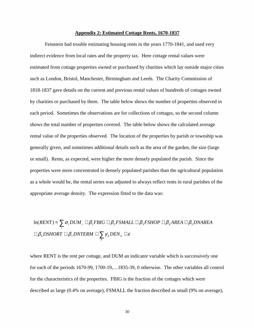
Appendix 2: Estimated Cottage Rents, 1670-1837

Feinstein had trouble estimating housing rents in the years 1770-1841, and used very

indirect evidence from local rates and the property tax. Here cottage rental values were

estimated from cottage properties owned or purchased by charities which lay outside major cities

such as London, Bristol, Manchester, Birmingham and Leeds. The Charity Commission of

1818-1837 gave details on the current and previous rental values of hundreds of cottages owned

by charities or purchased by them. The table below shows the number of properties observed in

each period. Sometimes the observations are for collections of cottages, so the second column

shows the total number of properties covered. The table below shows the calculated average

rental value of the properties observed. The location of the properties by parish or township was

generally given, and sometimes additional details such as the area of the garden, the size (large

or small). Rents, as expected, were higher the more densely populated the parish. Since the

properties were more concentrated in densely populated parishes than the agricultural population

as a whole would be, the rental series was adjusted to always reflect rents in rural parishes of the

appropriate average density. The expression fitted to the data was:

where RENT is the rent per cottage, and DUM an indicator variable which is successively one

for each of the periods 1670-99, 1700-19,…1835-39, 0 otherwise. The other variables all control

for the characteristics of the properties. FBIG is the fraction of the cottages which were

described as large (0.4% on average), FSMALL the fraction described as small (9% on average),

εγββ

βββββα

++++

+++++=

∑∑

kkk

ttt

DENDNTERMDSHORT

DNAREAAREAFSHOPFSMALLFBIGDUMRENT

76

54321)ln(

31

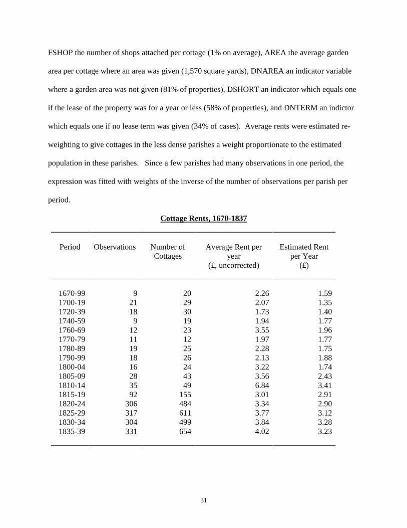
FSHOP the number of shops attached per cottage (1% on average), AREA the average garden

area per cottage where an area was given (1,570 square yards), DNAREA an indicator variable

where a garden area was not given (81% of properties), DSHORT an indicator which equals one

if the lease of the property was for a year or less (58% of properties), and DNTERM an indictor

which equals one if no lease term was given (34% of cases). Average rents were estimated re-

weighting to give cottages in the less dense parishes a weight proportionate to the estimated

population in these parishes. Since a few parishes had many observations in one period, the

expression was fitted with weights of the inverse of the number of observations per parish per

period.

Cottage Rents, 1670-1837

Period Observations Number ofCottages

Average Rent peryear

(£, uncorrected)

Estimated Rentper Year

(£)

1670-99 9 20 2.26 1.591700-19 21 29 2.07 1.351720-39 18 30 1.73 1.401740-59 9 19 1.94 1.771760-69 12 23 3.55 1.961770-79 11 12 1.97 1.771780-89 19 25 2.28 1.751790-99 18 26 2.13 1.881800-04 16 24 3.22 1.741805-09 28 43 3.56 2.431810-14 35 49 6.84 3.411815-19 92 155 3.01 2.911820-24 306 484 3.34 2.901825-29 317 611 3.77 3.121830-34 304 499 3.84 3.281835-39 331 654 4.02 3.23

32

Manuscript Sources on Wages

Day Wages

Beveridge Collection, Robbins Library, London School of Economics. Brooke, Isle of Wight (Box I11). DelisleAccounts (Box W2). Eton (Box I19). Pelham Papers (Box H12). Stowe Papers (Box H2). St Bartholomew’sHospital, Sandwich (Box E9). Winchester College (Box, --).

Bedford Record Office. Chester, BC 482, CH 938. Orlebar, OR 1372-4.Berkshire Record Office. Craven, D/E C A3. Throckmorton, D/E We A3, D/E We A5, D/E We A13.Buckinghampshire Record Office. Chester, D/C/2/45, D/C/2/52. Drake, D/DR/2/48, D/DR/2/51, D/DR/2/89,D/DR/2/164, D/DR/2/166, D/DR/2/168. Hampden, D/MH/30/5, D/MH/30/13, D/MH/30/15, D/MH/30/19,D/MH/30/21, D/MH/33/1-28.Cambridge Record Office. Cotton, 588/A2, 588/A4.Cumbria Record Office. Curwen, D/LONS, D/LONS/W3/14. Fleming, D/S/FLEMING/21. Pennington,D/PENN/202-4.Dorset Record Office. Bastard, 5339. Bragge, D 83/22. Damer, D188. Digby, KG 1229-40. Larder,PE/WCH/MI/1. Syndercombe, PE/SYM 2/5-6, KW 11A.Devon Record Office. Courtenay, 1508 M/V10, 1508 M/V31, 1508 M/V37. Crosse 1160M/Accounts A9(2)(Brampton). Drake 346 M/E2-11.Durham Record Office. Salvin, D/Sa/E167-177, D/Sa/E763-5.East Suffolk Record Office. Crowley, HA 1/GB3/2/1. Hill Farm, HA 2/B2/1. Labor Accounts, HA 2/B7/2, HA10/50/18/14, HA 30/369/41-43, HA 67/461/454.East Sussex Record Office. Ashburnham, ASH/1630. Shiffner, 1998, 3510. Stapley of Hickstead, HIC/467.Trevors of Glynde Place, GLY 2932-4.Essex Record Office. Bentall-Linnett, D/DE A1-2. Cook’s Farm, D/DU 441/52. Coopersale Hall, D/DU/363/4.Farm Accounts, D/DU/441/51-4. Gidea Hall, DDBe A1. Kempton, D/NM 1/1. Lennard, D/DL/E1, D/DL/E3.Petre, D/DP/A18-20, D/DP/A22, D/DP/A55, D/DP/A57, D/DP/A57, D/DP/A214. Tabor Family, D/DTa/A1.Tylers Hall, D/DM/A20, D/DM/A22. Ulnes Farm, D/DOp E 15. Watkinson, D/DU/224/2.Hampshire Record Office. Russell, 149M89/R5/6103, 149M89/R5/4613. Wheeler, 3m51/605.Hertford Record Office. Broadfield Hall, 70474A. Labor Accounts, D/ER96. Hatfield, 26294. Rolt,D/EAS/21710. Sebright, 18104. Wilshere, 61589.Huntingdon Record Office. Bernard, ddM5/4/1. Brampton, ddM5/5, ddMM/44D/7. Houghton, ddM/44D.Kent Record Office. Best, U480/E1-2. Croft, U709/A1. Darell, U386/A1. Gambia, U194/A8. Rockingham,U471/A18. Sackville, U269/A69/2, U269/A70/2, U269/A89. Tylden, U593/A7.Lancashire Record Office. Clifton, DDCI 399. Farington, DDF 31. Hesketh, DDHe/62/14-15, DDHe/62/25-29.Molyneaux, DDM/1/141.Leicester Record Office. Braye, Box III. Ferrers, 26D53/2335, 26D53/2465-6. Finch, DG7/1/37, DG7/1/43A.Herrick, DG9/2054. DE/814/3. DE667/70. Rothley, 2D31/241.Lincoln Record Office. Ancaster, 2 ANC. 7/7/53, 3 ANC. 6/24-25, 3 ANC. 9/15/165. Brace, 23/8/1. Monson,10/4B/13-20.Northampton Record Office. Dryden, D(CA) 307-8, D(CA) 312, D(CA) 323. Fitzwilliam Misc. Vols. 6, 8, 23, 50,74, 106-7, 157, 189, 191, 239, 790. Howe, YZ 997. Isham, IL 3945. Maxwell. Tryon, VII/619a-623. Wakefield,G2580/6.Nottingham Record Office. Arundle Castle, W114/8. Edge, DDE1/1-37. Franklin, DDF1/22, DDF1/122. Galway,12375/385. Middleton, MIAV/226. Nevile, DDN213/5. Newcastle, NEA444/1. Portland, DD4P/58/78, DD5P/1-150, DD5P/2/6-8, DD5P/4/1. Savile, DDSR/206/2, DDSR/211/257/1-22, DDSR/A4/49/1.Northumberland Record Office (Berwick). Haggeston, ZHG IV/3. Simpson, ZS1/1-4, ZS1/56-7, ZS1/94.Northumberland Record Office (Newcastle). Allgood, ZAL Box 44/1, Box 44/10, Box 60. Blackett, ZBH 273/2,ZBL 283/1- . Clark, ZCL.A. Hope-Wallace, ZHW/4/23. Swinburne, ZSW.Reading University Library. Wyche of Hockwold, NORF, 14/1/1.Sheffield City Library. Oakes, 1518.Somerset Record Office. Carew, DD/TB/Boxes 12-13, 14/6, 14/9, 14/11-12. Hylton DD/HY Box 12. Parsonage,DD/X/REE/C/1308. Popham DD/PO/32/2-97. Willoughby DD/WO/Box 49/10/pt 2.

33

Stafford Record Office. Bagot, D1721/F/61-66. Bradford, TP594. Gifford, D590/645-50. Hatherton,D260/M/E/86-97. D1788/143. Leveson-Gower, D593/F/2/18-35, D593/F/3/1/1-4, D593/F/3/25-27. Shrewsbury,D240/E/346-353, D240/E/463-472, D240/E/F/5/2. Sutherland, D593/L/---. Vernon, D1826/41.Surrey Record Office (Guildford). Howard, 1/53/4, 1/53/7-8. More-Molyneux, LM 1087/1/8, LM 1087/2/5/1, LM1087/2/16. Nicholas, 22/1/2. Shallet, 121/1/11/3. Wyatt, LM 1087/2/8, LM 1087/3/9, LM 1087/5/1-4.Warwick Record Office. Aylesford. Barker, CR233. Chesterfield, CR229/71. Conway, CR114A/292,CR114A/353, CR114A/357. Leigh, DR18/385. Northampton, CR556/275-6. Pleydell-Bourverie, 5476. Seymour,CR114A/202. Shirley, CR229/64.West Suffolk Record Office. Stanton Accounts, E1/11/2. Warner, 1341/5/2.West Sussex Record Office. Goodwood, E5422-5424, E5530-E5531.Westmoreland Record Office. Browne, WD/TE/Box 11/3.Wiltshire Record Office. Ashe, 118/140B, 118/141. Ballard, 1195/22. Blandy, 116/21. Burdett, 1883/192/1.Chippenham, 811/207. Duke of Somerset, 1332/Box 10. Enford, 415/86.Yorkshire Record Office (Sheepscar). Harewood, III 251. Ingram/Irwin, TN/EA/12/11. Robinson/Weddell, NH2187.

Payments for making faggots.

Beveridge Collection, Robbins Library, London School of Economics. Eton (Box I19). Pelham Papers (Box H12).

Cambridge Record Office. Cotton, 588/A2.Hertford Record Office. Broadfield Hall, 70474A.Leicester Record Office. Ferrers, 26D53/2465.Northampton Record Office. Fitzwilliam Misc. Vols. 8, 23, 74, 157, 189, 790. Howe, YZ 997.Somerset Record Office. Carew, DD/TB/Box 14/12. Hylton, DD/HY Box 12. Popham, DD/PO/32/2-97.Willoughby, DD/WO/Box 49/10/pt 2.Surrey Record Office (Guildford). More-Molyneux, LM 1087/2/16. Wyatt, LM 1087/2/8, LM 1087/5/1-4.

Threshing Payments:

Beveridge Collection, Robbins Library, London School of Economics. Stowe Papers (Box H2), St Bartholomew’sHospital, Sandwich (Box E9).

Bedford Record Office. Orlebar, OR 1372-4.Berkshire Record Office. Pleydell, D/E Pb E14, Throckmorton, D/E We A3, D/E We A5, D/E We A13.Buckinghampshire Record Office. Drake, D/DR/2/48.Dorset Record Office. Bragge, D 83/22.East Suffolk Record Office. Hill Farm, HA 2/B2/1. Labor Accounts, HA 10/50/18/14, HA 67/461/454.East Sussex Record Office. Shiffner, 1998, 3510. Trevors of Glynde Place, GLY 2932-4.Essex Record Office. Bentall-Linnett, D/DE A1-2. Farm Accounts, D/DU/441/51-4. Lennard, D/DL/E1, D/DL/E3.Petre, D/DP/A55, D/DP/A57, D/DP/A214. Tabor Family, D/DTa/A1. Tylers Hall, D/DM/A20, D/DM/A22.Watkinson, D/DU/224/2.Hampshire Record Office. Russell, 149M89/R5/6103.Hertford Record Office. Labor Accounts, D/ER96. Hatfield, 26294.Huntingdon Record Office. Bernard, ddM5/4/1. Brampton, ddM5/5, ddMM/44D/7. Houghton, ddM/44D.Manchester, ddM11/18.Leicester Record Office. Ferrers, 26D53/2465. Finch, DG7/1/37.Northampton Record Office. Fitzwilliam Misc. Vols. 6, 191. Isham, IL 3945.Nottingham Record Office. Portland, DD4P/58/78, DD5P/2/6-8, DD5P/4/1.Northumberland Record Office (Newcastle). Clark, ZCL.A.Reading University Library. Aveley, SAL 5/1/1.Somerset Record Office. Carew, DD/SAS/C/795/PR70, DD/TB/Boxes 13/4, 14/6, 14/11-12. Hylton DD/HY Box12. Willoughby DD/WO/Box 49/10/pt 2.Stafford Record Office. Leveson-Gower, D593/F/2/18, D593/F/2/24, D593/F/3/1/1, D593/F/3/25-26.

34

Surrey Record Office (Guildford). Howard, 1/53/4, 1/53/7-8. More-Molyneux, LM 1087/1/8, LM1087/1/10, LM1087/2/5/1, LM 1087/2/16. Wyatt, LM 1087/2/8.Warwick Record Office. Conway, CR114A/353, CR114A/357.West Suffolk Record Office. Stanton Accounts, E1/11/2. Warner, 1341/5/2.

Secondary Sources

Bacon, Richard N. 1844. The Report on the Agriculture of Norfolk. London: Ridgways and

Chapman and Hall.

Beveridge, Lord. 1939. Prices and Wages in England, Vol 1: The Mercantilist Era.

Bowden, Peter J. 1985. “Statistical Appendix,” in Joan Thirsk (ed.), The Agrarian History of

England and Wales, Vol. V.II, 827-902. Cambridge: Cambridge University Press.

Bowley, A. L. 1898. “The Statistics of Wages in the United Kingdom during the last Hundred

Years. Part I. Agricultural Wages,” Journal of the Royal Statistical Society, 61, 702-722.

Brassley, Paul, Anthony Lambert and Philip Saunders (eds.). 1988. Accounts of the Reverend

John Crakanthorp of Fowlmere, 1682-1710. Cambridge: Cambridge Record Society.

Clark, Gregory. 1991. "Labour Productivity in English Agriculture, 1300-1860," in B.M.S.

Campbell and Mark Overton, Agricultural Productivity in the European Past. Manchester:

Manchester University Press, 211-235.

Clark, Gregory. 1998a. “The Charity Commissioners as a Source in English Economic History”

Research in Economic History, 18 (1998), 1-52.

Clark, Gregory. 1998b. “Land Hunger: Land as a Commodity and as a Status Good in England,

1500-1910,” Explorations in Economic History, 35(1) (Jan., 1998), 59-82.

Clark, Gregory. 1998c. “Renting the Revolution” Journal of Economic History, 58(1) (March,

1998), 206-210.

Clark, Gregory and Ysbrand van der Werf. 1998. “Work in Progress. The Industrious

Revolution?” Journal of Economic History, 58(3) (September), 830-843.

35

Eccleston, Bernard. 1976. A Survey of Wage Rates in Five Midland Counties, 1750-1834.

Ph.D. Thesis, University of Leicester.

Feinstein, Charles. 1995. “Changes in Nominal Wages, the Cost of Living and Real Wages in the

United Kingdom over Two Centuries.” in P Scholliers and V. Zamagni (eds.), Labour’s Reward:

Real Wages and Economic Change in 19th- and 20th-Century Europe. Aldershot, Hants: Edward

Elgar.

Feinstein, Charles. 1998. “Pessimism Perpetuated: Real Wages and the Standard of Living in

Britain During and After the Industrial Revolution.” Journal of Economic History, 58 (3)

(Sept.), 625-658.

Fox, A. Wilson. 1903. “Agricultural Wages in England and Wales During the Last Half

Century.” Journal of the Royal Statistical Society, 46: 273-348.

Gardeners’ Chronicle and Agricultural Gazette. 1850. “The Value of Agricultural Labour,”

April 27, pp. 266-7.

Gilboy, Elizabeth W. 1932. “Labour at Thornborough: An Eighteenth Century Estate.”

Economic History Review, 3: 388-398.

Gilboy, Elizabeth W. 1934. Wages in Eighteenth Century England. Cambridge, Mass.: Harvard

University Press.

Harland, John (ed.). 1856. The House and Farm Accounts of the Shuttleworths of Gawthorpe

Hall. Parts 1 and 2. Chetham Society, 35 and 41.

Horrell, Sara. 1996. “Home Demand and British Industrialization.” Journal of Economic

History, 56 (3) (Sept.), 561-604.

36

John, A. H. 1989. “Statistical Appendix” in G. E. Mingay (ed.), The Agrarian History of

England and Wales, Vol. VI, 1750-1850, 1089-1177. Cambridge: Cambridge University Press.

Richardson, T. L. 1976. “The Agricultural Labourer’s Standard of Living in Kent 1790-1840.”

In Derek Oddy and Derek Miller (eds.), The Making of the Modern British Diet. London:

Croom Helm.

Richardson, T. L. 1977. The Standard of Living Controversy 1790-1840 with Special Reference

to Agricultural Labourers in Seven English Counties. Ph.D. Thesis, University of Hull.

Thorold Rogers, J. E. 1888b. A History of Agriculture and Prices in England. Volume 6.

Oxford: Clarendon Press.

Thorold Rogers, J. E. 1902. A History of Agriculture and Prices in England. Volume 7, Part 1.

Oxford: Clarendon Press.

Turner M.E., Beckett J.V., and B. Afton. 1996 “Taking Stock - Farmers, Farm Records, and

Agricultural Output in England, 1700-1850,” Agricultural History Review, 44(1): 21-34.

United Kingdom. House of Commons. 1834. Report on the Poor Laws in England and Wales,

Appendix (B), Part 1. Sessional Papers, Vol. 30.

United Kingdom. House of Lords. 1846. Vol. 23.

Young, Arthur. 1771a. A Six Months Tour Through the North of England. 2nd ed. London.

Young, Arthur. 1771b. A Farmer’s Tour through the East of England.

Young, Arthur. 1771c. A Six Weeks Tour Through the Southern Counties of England and

Wales. 3rd ed.