NGOs and the Effectiveness of Interventions

RUHRECONOMIC PAPERS

Faraz Usmani

Marc Jeuland

Subhrendu K. Pattanayak

#902

Imprint

Ruhr Economic Papers

Published by

RWI – Leibniz-Institut für Wirtschaftsforschung

Hohenzollernstr. 1-3, 45128 Essen, Germany

Ruhr-Universität Bochum (RUB), Department of Economics

Universitätsstr. 150, 44801 Bochum, Germany

Technische Universität Dortmund, Department of Economic and Social Sciences

Vogelpothsweg 87, 44227 Dortmund, Germany

Universität Duisburg-Essen, Department of Economics

Universitätsstr. 12, 45117 Essen, Germany

Editors

Prof. Dr. Thomas K. Bauer

RUB, Department of Economics, Empirical Economics

Phone: +49 (0) 234/3 22 83 41, e-mail: thomas.bauer@rub.de

Prof. Dr. Wolfgang Leininger

Technische Universität Dortmund, Department of Economic and Social Sciences

Economics – Microeconomics

Phone: +49 (0) 231/7 55-3297, e-mail: W.Leininger@tu-dortmund.de

Prof. Dr. Volker Clausen

University of Duisburg-Essen, Department of Economics

International Economics

Phone: +49 (0) 201/1 83-3655, e-mail: vclausen@vwl.uni-due.de

Prof. Dr. Ronald Bachmann, Prof. Dr. Manuel Frondel, Prof. Dr. Torsten Schmidt,

Prof. Dr. Ansgar Wübker

RWI, Phone: +49 (0) 201/81 49-213, e-mail: presse@rwi-essen.de

Editorial Office

Sabine Weiler

RWI, Phone: +49 (0) 201/81 49-213, e-mail: sabine.weiler@rwi-essen.de

Ruhr Economic Papers #902

Responsible Editor: Manuel Frondel

All rights reserved. Essen, Germany, 2021

ISSN 1864-4872 (online) – ISBN 978-3-96973-043-0

The working papers published in the series constitute work in progress circulated to stimulate

discussion and critical comments. Views expressed represent exclusively the authors’ own opinions

and do not necessarily reflect those of the editors.

Ruhr Economic Papers #902

Faraz Usmani, Marc Jeuland, and Subhrendu K. Pattanayak

NGOs and the Effectiveness of Interventions

Bibliografische Informationen

der Deutschen Nationalbibliothek

The Deutsche Nationalbibliothek lists this publication in the Deutsche National bibliografie;

detailed bibliographic data are available on the Internet at http://dnb.dnb.de

RWI is funded by the Federal Government and the federal state of North Rhine-Westphalia.

http://dx.doi.org/10.4419/96973043

ISSN 1864-4872 (online)

ISBN 978-3-96973-043-0

Faraz Usmani, Marc Jeuland, and Subhrendu K. Pattanayak1

NGOs and the Effectiveness of Interventions

Abstract

Interventions led by non-governmental organizations (NGOs) are often more effective than

comparable efforts by other actors, yet relatively little is known about how implementer identity

drives final outcomes. Combining a stratified field experiment in India with a triple-differences

estimation strategy, we show that a local development NGO’s prior engagement with target

communities increases the effectiveness of a technology-promotion intervention implemented

by it by at least 30 percent. This “NGO effect” has implications for the generalizability and

scalability of evidence from experimental research conducted with local implementation

partners.

JEL-Code: L31, C93, O12, O17

Keywords: NGOs; field experiments; external validity

March 2021

1 Faraz Usmani, Mathematica; Marc Jeuland, Duke University and RWI; Subhrendu K. Pattanayak, Duke University. - We thank Chris Barrett, Anna Birkenbach, Laura Grant, Esther Heesemann, David Kaczan, Timur Kuran, Brian Murray, Jennifer Orgill-Meyer, Jörg Peters, Seth Sanders, and seminar participants at AERE 2016, SEA 2016, CECFEE 2016, EAERE 2017, the University of Gothenburg, the 2017 Occasional Workshop in Environmental and Resource Economics, EfD 2017, CSAE 2018, WCERE 2018, RWI–Leibniz Institute for Economic Research, Cornell University and MWIEDC 2020 for valuable comments. This study was made possible by the support of the American people through the United States Agency for International Development (USAID), and was partially funded by USAID under Translating Research into Action, Cooperative Agreement No GHS-A-00-09-00015-00. The contents of this publication are the sole responsibility of the authors and do not necessarily reflect the views of USAID or the United States Government. Usmani also gratefully acknowledges support from the Duke Global Health Institute, Duke University Energy Initiative, Sustainable Energy Transitions Initiative, the United Nations University World Institute for Development Economics Research, and the Cornell Atkinson Center for Sustainability. The field experiment described in this study is registered in the AEA Registry for Randomized Controlled Trials (AEARCTR-0003400). The study protocol was reviewed and approved by Duke University’s Institutional Review Board (IRB Protocol No A0946); informed consent was obtained from all participating households. Any remaining errors are our own. – All correspondence to: Faraz Usmani, Research Economist, International Unit, Mathematica, e-mail: fusmani@mathematica-mpr.com

1 Introduction

Implementation challenges stymie policies and programs in virtually every sector. Transaction

costs borne to identify beneficiaries and service providers, gauge their trustworthiness, bargain to

reach consensus, and monitor agreements to ensure they are fulfilled can undermine the effective-

ness of interventions—particularly in low-income settings, in which such frictions are especially

important (e.g., Holloway et al., 2000; Ito, 2009; Jack and Suri, 2014). Where public-service

delivery has proven difficult, a variety of non-state, non-market institutions—most notably

nongovernmental organizations (NGOs)—have emerged (Besley and Ghatak, 2017; Brass et al.,

2018; Werker and Ahmed, 2008).1 That they are (at least in theory) nimble and efficient has

made them attractive partners for international donors (Brass, 2016). In 2012, for instance,

Organisation for Economic Co-operation and Development (OECD) countries channelled over

$17 billion of overseas development assistance to—and through—NGOs (Aldashev and Navarra,

2018). Private charitable giving to international development NGOs may be considerably higher

(Micklewright and Wright, 2003). Yet little is known about the ways in which NGOs directly

impact the effectiveness of the interventions they implement.

In this study, we develop a model of household decision-making to consider how NGOs

reduce transactions costs and influence intervention outcomes. We then use a novel matched–

experimental study design to test our model’s main theoretical claim: that an NGO lowers

transaction costs where it has previously been more active, which in turn increases intervention

effectiveness. We test this claim in the context of an intervention designed to promote improved

cookstoves (ICS) in rural India. Nearly three billion people globally rely on traditional stoves

and solid fuels for their primary energy needs. ICS, which are designed to increase the efficiency

of solid-fuel combustion, have long been seen as a potential solution to the environmental–

health–development burden these energy-use patterns impose (Jeuland and Pattanayak, 2012).2

1By some estimates, India alone is home to over three million of them—a figure that outnumbers its publichospitals, schools, and police force (Anand, 2015). In contrast, the total number of international NGOs is moreconservatively estimated to be closer to 30,000 (Aldashev and Navarra, 2018).

2Reliance on traditional fuels and stoves imposes a tremendous burden on household health (via exposure tohousehold air pollution); local forests (via unsustainable extraction of fuelwood); and the global climate (dueto widespread biomass burning). Bailis et al. (2015), Jeuland and Pattanayak (2012), Jeuland et al. (2015), andVenkataraman (2005) provide an overview of the global nature and magnitude of these environmental, health, andwelfare challenges.

1

Yet widespread uptake has proven challenging (e.g., Mobarak et al., 2012) and—as in other

arenas—the role played by local institutions in driving adoption remains poorly understood

despite considerable scholarship on other factors that encourage or limit uptake (Lewis and

Pattanayak, 2012).

We first use ex ante matching to create two observationally similar sub-samples of villages

that are differentiated only by prior exposure to a local development NGO. In partnership with

this NGO, we then implement a stratified, cluster randomized controlled trial (RCT) designed to

evaluate the effectiveness of an ICS-promotion campaign in nearly 100 geographically distinct

hamlets within these villages, covering a sample of almost 1,000 households. Our results suggest

that the intervention increases adoption: nearly half of all households targeted by the promotion

campaign purchased an ICS. However, our study design also allows us to identify heterogeneity

in the effectiveness of the NGO in spurring ICS adoption. We uncover a large, positive, and

statistically significant “NGO effect”: purchase rates are approximately 14 percentage points

(31 percent) higher in treated communities with prior interactions with the NGO. Robustness

checks reveal that this finding is not sensitive to different ways of defining the scope of the

NGO’s prior relationships with communities. It is also highly unlikely to have been driven by

the chance selection of the set of villages in our sample, as revealed by placebo tests inspired by

randomization-based inferential procedures.

Using a triple-differences specification—which further relaxes our identifying assumptions,

and allows us to isolate the causal impact of the NGO on the effectiveness of the intervention—

we find that treated households in NGO communities are also 16 percentage points more likely

to continue to own and use intervention stoves over time than treated households in communities

without a prior relationship with the NGO, representing a 50–80 percent increase in the size of

the treatment effect. Consistent with these patterns of adoption and use, treated households in

NGO communities exhibit significant reductions in the use of solid fuels and in fuel-collection

times. In contrast, we find no evidence of similar improvements in energy-use patterns for

treated households in non-NGO communities. Our stratified study design, therefore, reveals that

we would have considerably overestimated the effectiveness of our intervention had it been a

typical randomized evaluation conducted in partnership with the NGO. This is because such

2

evaluations are generally implemented within an implementer’s existing sphere of influence.

These findings highlight a relatively unacknowledged aspect of the rise of NGOs as partners

in applied research, especially in recent years in response to growing calls for more “evidence-

based” policies (Banerjee et al., 2007, 2017). Charity evaluators (such as GiveWell and Giving

What We Can) routinely release lists of top NGOs whose effectiveness is rigorously evaluated

for would-be donors in search of causes. In the fiercely competitive world of fund-raising,

such signals do not go unnoticed, and NGOs are often keen to work with researchers and

have the impacts of their programs assessed. For applied researchers, partnerships with NGOs

provide ready access to target populations, local expertise, and human resources and operational

infrastructure, all of which lower the costs of doing research and create opportunities for

researchers to test new theories directly. RCTs in low- and middle-income countries have

particularly benefited from these collaborations. Indeed, proponents argue that “many of the

best RCTs have come from long-term partnerships between researchers and NGOs or other

local partners” (Glennerster, 2015). NGO–researcher collaborations undoubtedly yield valuable

insights about the effectiveness of environmental, health, and development interventions (e.g.,

Banerjee et al., 2015; Brooks et al., 2016; Jayachandran et al., 2017; Miguel and Kremer, 2004).

That said, we show that this seemingly symbiotic relationship may also mask the unique roles

NGOs often play in remote, rural settings—with major implications for the generalizability and

scalability of solutions deemed effective in applied research (Barrett and Carter, 2014; Peters

et al., 2018; Vivalt, 2020).

More broadly, our study is motivated by calls for research that sheds light on how and why

certain interventions are effective, not simply whether or not they are (Deaton, 2010; Pattanayak

et al., 2017; Rosenthal et al., 2017). In particular, we demonstrate how solutions from applied

research that is tied to the places, populations, and programs associated with specific NGOs

may have very different impacts when implemented in alternative settings (Ravallion, 2009).3

3This is often referred to as “site selection bias” (Allcott, 2015) and can arise in at least two different ways.First, as Lin et al. (2012) show in the context of forestry interventions, the spatial distribution of social-welfareprograms is non-random. The presence of such programs for the purposes of evaluation is correlated with pastlevels of NGO activity, which is itself strategically determined by NGOs (Aldashev et al., 2014, 2020; Brass, 2012;Fruttero and Gauri, 2005; MacLean et al., 2015). Second, NGOs capable of managing complex RCTs (designedto provide evidence of program effectiveness) are also likely to implement programs more effectively than theaverage implementer. Such “persistent productivity differentials,” whereby organizations confronting seeminglysimilar circumstances sometimes perform at persistently different levels, have been documented in a number of

3

Our study is also related to a growing literature on the role of implementer identity, which

finds that NGO-led interventions are generally more effective than comparable efforts by other

actors (Berge et al., 2012; Bold et al., 2018; Cameron et al., 2019; Grossman et al., 2020;

Henderson and Lee, 2015).4 Yet such comparisons implicitly assume that there is something

inherently different about NGOs that leads to implementation effectiveness. As we show, this

is not necessarily the case, and even heretofore “effective” NGOs may struggle to overcome

implementation-related barriers when operating in new settings in which their stock of social

capital is low. This is because effective local NGOs often spend years fostering trust in the

communities in which they operate. These typically unobserved context- and NGO-specific

characteristics interact with aspects of the intervention, influence transaction costs associated

with implementation, and ultimately help determine final outcomes.5 Policymakers looking to

scale-up interventions with demonstrable impact to new settings must be cognizant of the ways

in which proposed policies will interact with these contextual factors, and not simply assume

that prior successes will be guaranteed (Woolcock et al., 2011).

Nevertheless, we recognize that ours is not the only study grappling with these questions,

and that there are tangible opportunities for us to incorporate lessons from the broader literature

on the importance of implementer identity. To evaluate the relative strength of the evidence we

uncover, and to see how it builds on and shapes the collective knowledge in this domain, we apply

a simple Bayesian framework. First, we use estimates from Bold et al. (2018) and Cameron et al.

(2019)—who compare the effectiveness of an NGO-led intervention to a government-led one—

to formally specify a distribution for our prior understanding of the effects NGOs might have on

final outcomes. We then ask: how does our study add to this prior knowledge? To answer this

question, we use this prior distribution as a critical component of a multilevel Bayesian analysis,

and show that a synthesis of existing insights with our results yields posterior distributions of the

other settings in organizational economics (Gibbons, 2010).4A separate but related body of work explores the comparative advantages non-profit organizations (including

NGOs) have relative to for-profit firms. Francois (2001, 2003), for instance, argues that non-profits are moreeffective at securing care-motivated effort—in addition to pecuniarily motivated effort—from workers. Besleyand Ghatak (2001) extend this literature by developing a theoretical model that considers scenarios under whichgovernments or private organizations should own public projects, which shows that the “more caring party shouldbe the owner of a public project irrespective of comparative advantage in the production of the service.”

5For instance, if beneficiaries are unsure about the benefits and costs associated with unfamiliar welfare-improving technologies (such as ICS), trusted NGOs can leverage these relationships to reduce households’perceptions of the risks associated with technology adoption.

4

magnitude of the “NGO effect” that are considerably more precise. Importantly, we demonstrate

that the results of this exercise overwhelmingly point to this effect being positive.

This paper proceeds as follows: in Section 2, we develop a theoretical model of household

decision-making in the presence of NGOs and transaction costs; Section 3 provides an overview

of our data and sample-selection methods; Section 4 outlines our empirical framework and

identification strategy; Section 5 presents results; Section 6 demonstrates how insights from the

related literature inform our results within a Bayesian framework; and Section 7 concludes.

2 NGOs, transaction costs, and household decision-making

Transaction costs are inherent in the adoption of new technologies—especially in remote, rural

settings characterized by low information (Bernard et al., 2017; Foster and Rosenzweig, 2010;

Suri, 2011). For example, while the material costs of new technologies are usually borne

immediately, benefits are often uncertain and realized far in the future; resources are thus

required to learn about the valuable attributes of the technology, and gauge the full extent of its

costs and benefits. In addition, the search and exchange process that technology adoption entails

can impose significant costs. These are often related to the size of the market. Relatively large

markets—such as major urban areas—feature a multitude of retailers and suppliers, competing

along technology price, quality, and differentiability criteria. In contrast, relatively small

markets—such as remote, rural settings—are characterized by weak supply chains, a paucity of

suppliers, and limited options. These contextual characteristics influence households’ decisions

about technology adoption, particularly in smaller markets in which kinship ties, reciprocal

exchange, and repeated dealings (in other words, social capital) are more salient (Kranton,

1996).

These insights motivate our model of household decision-making. Drawing on Jeuland

et al. (2015)—who in turn build on more fundamental work in environmental and health

economics (Grossman, 1972; Pattanayak and Pfaff, 2009)—we develop a model in which

households decide whether to invest in technologies that avert environmental health risks (such

as ICS). These decisions necessarily involve a trade-off with consumption of other goods and

5

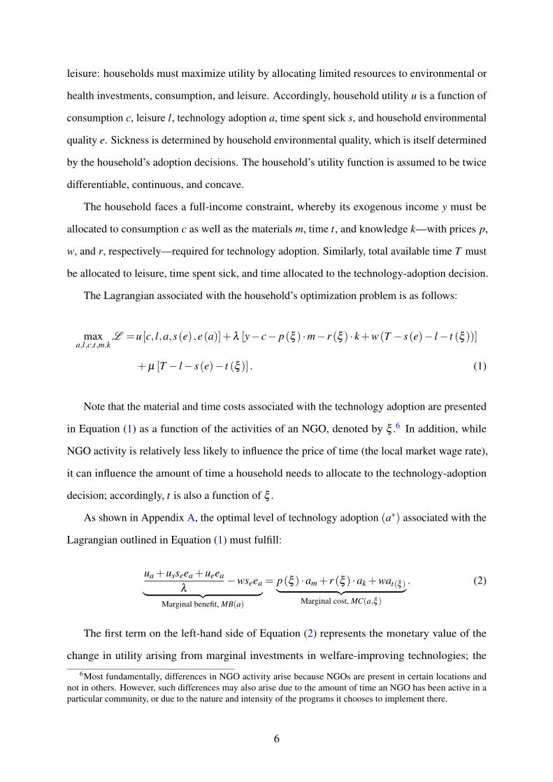
leisure: households must maximize utility by allocating limited resources to environmental or

health investments, consumption, and leisure. Accordingly, household utility u is a function of

consumption c, leisure l, technology adoption a, time spent sick s, and household environmental

quality e. Sickness is determined by household environmental quality, which is itself determined

by the household’s adoption decisions. The household’s utility function is assumed to be twice

differentiable, continuous, and concave.

The household faces a full-income constraint, whereby its exogenous income y must be

allocated to consumption c as well as the materials m, time t, and knowledge k—with prices p,

w, and r, respectively—required for technology adoption. Similarly, total available time T must

be allocated to leisure, time spent sick, and time allocated to the technology-adoption decision.

The Lagrangian associated with the household’s optimization problem is as follows:

maxa,l,c,t,m,k

L =u [c, l,a,s(e) ,e(a)]+λ [y− c− p(ξ ) ·m− r (ξ ) · k+w(T − s(e)− l − t (ξ ))]

+µ [T − l − s(e)− t (ξ )] . (1)

Note that the material and time costs associated with the technology adoption are presented

in Equation (1) as a function of the activities of an NGO, denoted by ξ .6 In addition, while

NGO activity is relatively less likely to influence the price of time (the local market wage rate),

it can influence the amount of time a household needs to allocate to the technology-adoption

decision; accordingly, t is also a function of ξ .

As shown in Appendix A, the optimal level of technology adoption (a∗) associated with the

Lagrangian outlined in Equation (1) must fulfill:

ua +usseea +ueea

λ−wseea

︸ ︷︷ ︸

Marginal benefit, MB(a)

= p(ξ ) ·am + r (ξ ) ·ak +wat(ξ )︸ ︷︷ ︸

Marginal cost, MC(a,ξ )

. (2)

The first term on the left-hand side of Equation (2) represents the monetary value of the

change in utility arising from marginal investments in welfare-improving technologies; the

6Most fundamentally, differences in NGO activity arise because NGOs are present in certain locations andnot in others. However, such differences may also arise due to the amount of time an NGO has been active in aparticular community, or due to the nature and intensity of the programs it chooses to implement there.

6

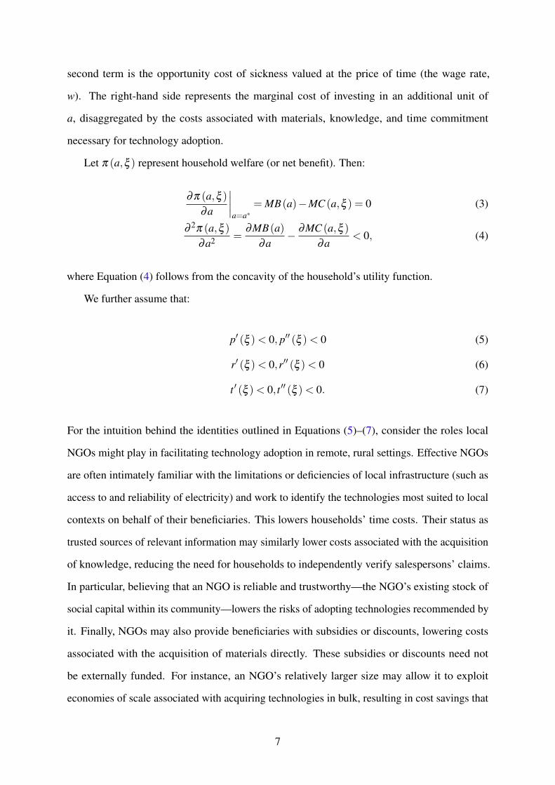
second term is the opportunity cost of sickness valued at the price of time (the wage rate,

w). The right-hand side represents the marginal cost of investing in an additional unit of

a, disaggregated by the costs associated with materials, knowledge, and time commitment

necessary for technology adoption.

Let π (a,ξ ) represent household welfare (or net benefit). Then:

∂π (a,ξ )

∂a

∣∣∣∣a=a∗

= MB(a)−MC (a,ξ ) = 0 (3)

∂ 2π (a,ξ )

∂a2 =∂MB(a)

∂a−

∂MC (a,ξ )

∂a< 0, (4)

where Equation (4) follows from the concavity of the household’s utility function.

We further assume that:

p′ (ξ )< 0, p′′ (ξ )< 0 (5)

r′ (ξ )< 0,r′′ (ξ )< 0 (6)

t ′ (ξ )< 0, t ′′ (ξ )< 0. (7)

For the intuition behind the identities outlined in Equations (5)–(7), consider the roles local

NGOs might play in facilitating technology adoption in remote, rural settings. Effective NGOs

are often intimately familiar with the limitations or deficiencies of local infrastructure (such as

access to and reliability of electricity) and work to identify the technologies most suited to local

contexts on behalf of their beneficiaries. This lowers households’ time costs. Their status as

trusted sources of relevant information may similarly lower costs associated with the acquisition

of knowledge, reducing the need for households to independently verify salespersons’ claims.

In particular, believing that an NGO is reliable and trustworthy—the NGO’s existing stock of

social capital within its community—lowers the risks of adopting technologies recommended by

it. Finally, NGOs may also provide beneficiaries with subsidies or discounts, lowering costs

associated with the acquisition of materials directly. These subsidies or discounts need not

be externally funded. For instance, an NGO’s relatively larger size may allow it to exploit

economies of scale associated with acquiring technologies in bulk, resulting in cost savings that

7

it can pass onto its beneficiaries.7

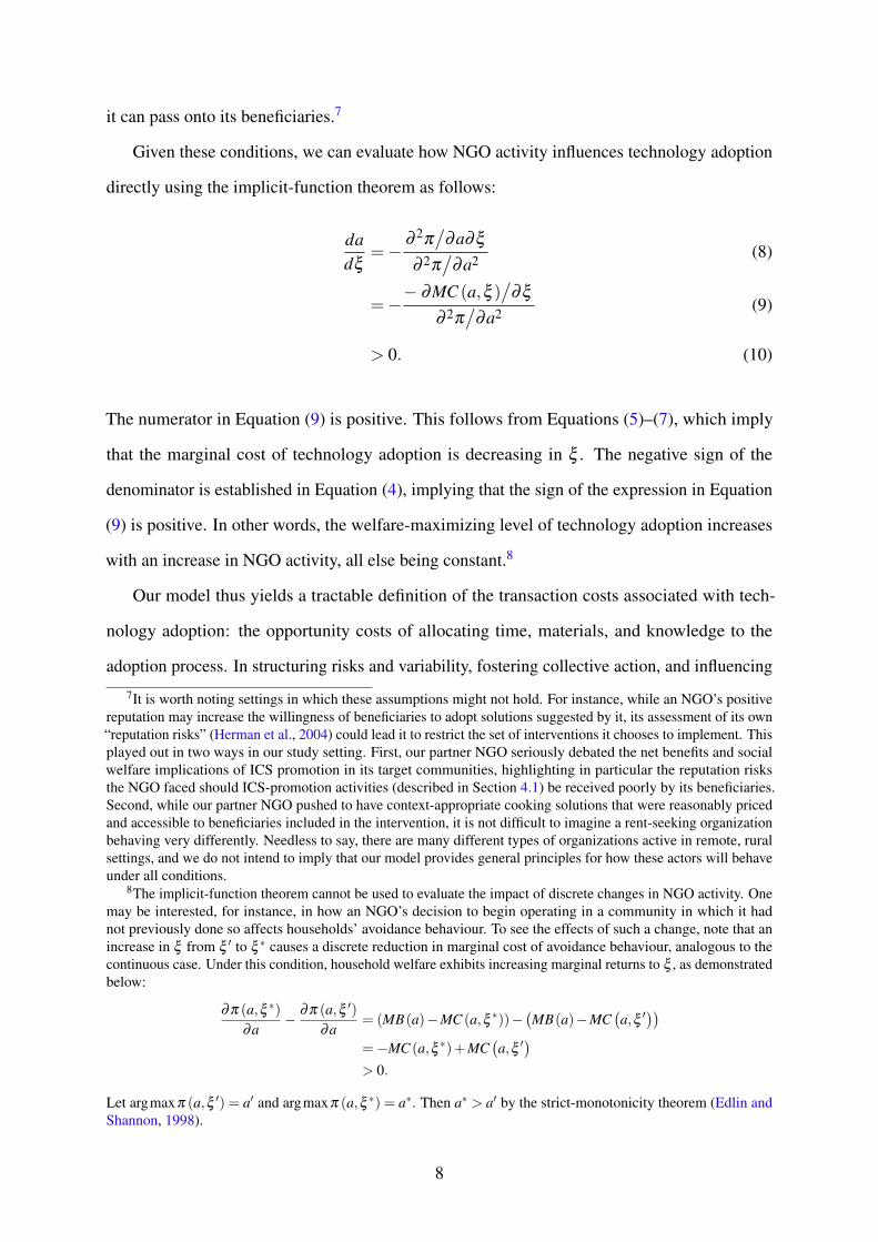
Given these conditions, we can evaluate how NGO activity influences technology adoption

directly using the implicit-function theorem as follows:

da

dξ=−

∂ 2π/

∂a∂ξ

∂ 2π/

∂a2(8)

=−− ∂MC (a,ξ )

/∂ξ

∂ 2π/

∂a2(9)

> 0. (10)

The numerator in Equation (9) is positive. This follows from Equations (5)–(7), which imply

that the marginal cost of technology adoption is decreasing in ξ . The negative sign of the

denominator is established in Equation (4), implying that the sign of the expression in Equation

(9) is positive. In other words, the welfare-maximizing level of technology adoption increases

with an increase in NGO activity, all else being constant.8

Our model thus yields a tractable definition of the transaction costs associated with tech-

nology adoption: the opportunity costs of allocating time, materials, and knowledge to the

adoption process. In structuring risks and variability, fostering collective action, and influencing

7It is worth noting settings in which these assumptions might not hold. For instance, while an NGO’s positivereputation may increase the willingness of beneficiaries to adopt solutions suggested by it, its assessment of its own“reputation risks” (Herman et al., 2004) could lead it to restrict the set of interventions it chooses to implement. Thisplayed out in two ways in our study setting. First, our partner NGO seriously debated the net benefits and socialwelfare implications of ICS promotion in its target communities, highlighting in particular the reputation risksthe NGO faced should ICS-promotion activities (described in Section 4.1) be received poorly by its beneficiaries.Second, while our partner NGO pushed to have context-appropriate cooking solutions that were reasonably pricedand accessible to beneficiaries included in the intervention, it is not difficult to imagine a rent-seeking organizationbehaving very differently. Needless to say, there are many different types of organizations active in remote, ruralsettings, and we do not intend to imply that our model provides general principles for how these actors will behaveunder all conditions.

8The implicit-function theorem cannot be used to evaluate the impact of discrete changes in NGO activity. Onemay be interested, for instance, in how an NGO’s decision to begin operating in a community in which it hadnot previously done so affects households’ avoidance behaviour. To see the effects of such a change, note that anincrease in ξ from ξ ′ to ξ ∗ causes a discrete reduction in marginal cost of avoidance behaviour, analogous to thecontinuous case. Under this condition, household welfare exhibits increasing marginal returns to ξ , as demonstratedbelow:

∂π (a,ξ ∗)

∂a−

∂π (a,ξ ′)

∂a= (MB(a)−MC (a,ξ ∗))−

(MB(a)−MC

(a,ξ ′

))

=−MC (a,ξ ∗)+MC(a,ξ ′

)

> 0.

Let argmaxπ (a,ξ ′) = a′ and argmaxπ (a,ξ ∗) = a∗. Then a∗ > a′ by the strict-monotonicity theorem (Edlin andShannon, 1998).

8

existing practices, NGOs alter the set of costs associated with investments in welfare-improving

technologies—and, indeed, of participating in environmental, health, and development interven-

tions more broadly. Recent work has looked at the roles NGOs play in enhancing monitoring

and enforcement (Aldashev et al., 2015; Grant and Grooms, 2017); improving public-service de-

livery (Devarajan et al., 2013); and working with heterogeneous beneficiaries (Bengtsson, 2013).

Outside of a nascent stream of research on the strategic nature of NGOs’ location decisions

(Brass, 2012; Fruttero and Gauri, 2005; MacLean et al., 2015), however, little is known about the

roles that they might play in directly determining the outcomes of applied interventions. Indeed,

while some have noted the presence of differential impacts across communities with and without

NGO activity (e.g., Jeuland et al., 2020; Johnson-Lans, 2008; Niehaus and Sukhtankar, 2013;

Sharma et al., 2015), to the best of our knowledge no study has rigorously examined how the

presence of an effective local NGO and the specific institutional context that represents might

directly influence household decision-making. In contrast, our model provides a clear, empiri-

cally testable hypothesis: where NGO activity has been higher, intervention effectiveness—in

our case, in the form of uptake of ICS technologies—will also be higher. The remainder of this

paper turns to an empirical evaluation of this claim.

3 Data and descriptive statistics

Our sampling frame consists of over 1,000 households across 97 geographically distinct hamlets

(toks) located in 38 Census-delineated villages (gram panchayats) in the northern Indian state of

Uttarakhand. In this section we (i) describe the creation of observationally equivalent groups

of these 38 NGO and non-NGO villages using ex-ante propensity score matching; (ii) explain

our procedure for random selection of participant households in hamlets located within these

villages; and (iii) present descriptive statistics for our final sample of households.

3.1 Creation of NGO and non-NGO strata

Given our interest in the influence of community-level institutional factors—as well as the fact

that interventions are often initiated at the community level—we developed a sampling strategy

9

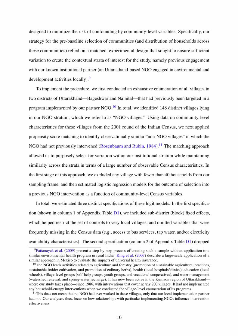
designed to minimize the risk of confounding by community-level variables. Specifically, our

strategy for the pre-baseline selection of communities (and distribution of households across

these communities) relied on a matched–experimental design that sought to ensure sufficient

variation to create the contextual strata of interest for the study, namely previous engagement

with our known institutional partner (an Uttarakhand-based NGO engaged in environmental and

development activities locally).9

To implement the procedure, we first conducted an exhaustive enumeration of all villages in

two districts of Uttarakhand—Bageshwar and Nainital—that had previously been targeted in a

program implemented by our partner NGO.10 In total, we identified 148 distinct villages lying

in our NGO stratum, which we refer to as “NGO villages.” Using data on community-level

characteristics for these villages from the 2001 round of the Indian Census, we next applied

propensity score matching to identify observationally similar “non-NGO villages” in which the

NGO had not previously intervened (Rosenbaum and Rubin, 1984).11 The matching approach

allowed us to purposely select for variation within our institutional stratum while maintaining

similarity across the strata in terms of a large number of observable Census characteristics. In

the first stage of this approach, we excluded any village with fewer than 40 households from our

sampling frame, and then estimated logistic regression models for the outcome of selection into

a previous NGO intervention as a function of community-level Census variables.

In total, we estimated three distinct specifications of these logit models. In the first specifica-

tion (shown in column 1 of Appendix Table D1), we included sub-district (block) fixed effects,

which helped restrict the set of controls to very local villages, and omitted variables that were

frequently missing in the Census data (e.g., access to bus services, tap water, and/or electricity

availability characteristics). The second specification (column 2 of Appendix Table D1) dropped

9Pattanayak et al. (2009) present a step-by-step process of creating such a sample with an application to asimilar environmental health program in rural India. King et al. (2007) describe a large-scale application of asimilar approach in Mexico to evaluate the impacts of universal health insurance.

10The NGO leads activities related to agriculture and forestry (promotion of sustainable agricultural practices,sustainable fodder cultivation, and promotion of culinary herbs), health (local hospitals/clinics), education (localschools), village-level groups (self-help groups, youth groups, and vocational cooperatives), and water management(watershed renewal, and spring-water recharge). It has now been active in the Kumaon region of Uttarakhand—where our study takes place—since 1986, with interventions that cover nearly 200 villages. It had not implementedany household-energy interventions when we conducted the village-level enumeration of its programs.

11This does not mean that no NGO had ever worked in these villages, only that our local implementation partnerhad not. Our analyses, thus, focus on how relationships with particular implementing NGOs influence interventioneffectiveness.

10

these sub-district fixed effects, whereas the third specification (column 3 of Appendix Table D1)

was similar to the second except that it included the additional controls (with missing values in

the Census assumed to be zero, or omitted in the case of tap-water availability). We eliminated

the second specification because it was clearly less robust to the distance restrictions for our

sample, that is, fewer matches were preserved when dropping the sub-districts far away from

our base of operations. We also found that the quality of matches on a number of variables was

greatly reduced with inclusion of the sub-district-level controls used in the first specification.

Thus, our final strata-creation exercise is based on the third specification. This first stage reveals

that, in general, NGO villages are slightly smaller and have proportionally more Scheduled

Caste members than the average village.12 NGO villages are also more likely to have infras-

tructure or village-level institutions (schools, credit societies, and bus facilities), but are more

remote (further away from large towns, and with less access to paved roads and telephones) than

non-NGO villages.

In the second stage, following the logit estimation, we estimated the probability of receiving a

previous NGO intervention for all villages in our eligible districts. These predicted probabilities

constitute the propensity score for each village. We matched NGO villages to non-NGO villages

with the most similar propensity scores, allowing for replacement, and limiting matches to the

support region with the greatest overlap in density of NGO and non-NGO villages (Appendix

Figure C1). In this way, we ensured that the communities selected for our sampling frame were

as similar as possible. For each model, we developed a matching routine that restricted our

potential sample villages on the basis of size (greater than 40 households) and distance from

the base of operations for our survey (working in sub-districts that could be reached within

one day). We next eliminated the worst 10 percent of matches on the basis of propensity score

distance—a process known as “trimming”—to ensure that pairs that were poor matches would

not be selected simply due to the inclusion of villages that did not happen to have good matches

(Crump et al., 2009).

Finally, to draw our precise sample of matched pairs, we studied each of the individual

pairs remaining after trimming in detail. Here, we paid particular attention to match quality and

12The Scheduled Castes and Scheduled Tribes are various historically disadvantaged or indigenous groups inIndia that have received official recognition as such from the Indian government.

11

overall balance between the NGO and non-NGO strata with regards to key contextual factors

(such as population, distance from nearby towns, and the presence of village-level groups and

societies). Our final sample consisted of 38 villages (19 matched pairs of NGO and non-NGO

villages). At the conclusion of our matching exercise, our matched pairs of NGO and non-NGO

villages were balanced on all community-level characteristics used during our propensity-score

estimation (Table 1).13

3.2 Sub-cluster survey samples and household surveys

Uttarakhand is one of India’s least densely populated states, with terrain that gives rise to

“sub-clusters” (geographically distinct hamlets known as toks) within villages.14 These hamlets

typically vary in terms of cultural and socioeconomic characteristics. To maximize sample

variation along these socioeconomic lines, we randomly selected between two and four hamlets

within each matched village for our final sample. Specifically, we determined that our survey

teams would work within at least two hamlets in small villages, at least three in medium villages,

and at least four in large villages (owing to population differences across these three groups of

villages). Our final sample consisted of 97 hamlets.

Households within hamlets were randomly selected to participate in survey activities; base-

line surveys occurred during the summer of 2012.15 If household members were unavailable

during the entire day of survey activities—or if they refused to participate—neighbouring

households were randomly selected as replacements. Field supervisors performed household

introductions and obtained informed consent, recorded GPS coordinates and elevation data, and

oversaw quality-control checks in each village. A random subsample of households was also

13Appendix Table D2 presents additional tests of cross-sectional balance using more detailed community-leveldata from the 2011 round of the Indian Census. We did not use this Census round for our matching exercise asit had only been released provisionally at the time. Nevertheless, we find that NGO and non-NGO villages arebalanced across multiple dimensions using these data as well.

14Topographically, Uttarakhand is characterized by “hilly terrain, rugged and rocky mountains, deep valleys,high peaks, swift streams and rivulets, rapid soil erosion, frequent landslides and widely scattered habitation”(Maurya, 2014).

15Highly variable village structures and geographic constraints created variation in the number of hamlets andhouseholds sampled in each village. A minimum of 20 household surveys were completed in small villages, 30in medium ones, and 40 in large ones. If a village was divided into distinct geographical sub-units (e.g., half thevillage was to the north of the main road, while the other half was to the south), the target number of surveys wassplit equally among these groups.

12

selected for detailed weighing of daily solid-fuel use.16

The ICS-promotion intervention (described in detail in Section 4.1) began in August 2013,

with midline and endline surveys taking place around November 2013 and November 2014—the

three- and fifteen-month marks, respectively.

3.3 Descriptive statistics

Table 2 presents an overview of our main sample of 943 households, disaggregated by NGO and

non-NGO villages.17 The average household in our study consisted of just under five members

at baseline. The average household head was 54 years old and had completed approximately

six years of formal education. Only about one-quarter of surveyed households were headed by

women, and more than half fell below the Indian poverty line.

As in many other parts of rural India, reliance on traditional stoves and fuels was nearly

universal.18 In contrast, only about one-third of households owned any type of improved stove

at baseline; this was almost exclusively limited to liquefied petroleum gas (LPG) stoves, which

are typically owned by relatively wealthy households. Awareness of modern alternatives to

traditional cooking technologies was low: only about one-quarter to one-third of households

professed an awareness of the existence of stoves or fuels that produce less smoke. This was not

necessarily due to a lack of awareness about the harms associated with exposure to household

air pollution. Indeed, half of surveyed households believed that the smoke generated by their

primary stove was unsafe. Households also reported spending up to two hours per day on

average collecting traditional fuels for household use. In addition, around one in five households

reported that at least one family member suffered from a case of cough or cold in the two weeks

prior to the survey. Together, this suggests that the welfare burden imposed by widespread

16This process involves asking households to collect an amount of fuelwood and other solid fuels that is slightlymore than what they anticipate using over the next day. This amount is weighed by the field team, which returnsapproximately 24 hours later to weigh the remaining amount.

17We interviewed approximately 1,050 households at baseline. We restrict our main analytical sample to the 943households that were also located and interviewed during the midline (three-month) and endline (fifteen-month)survey rounds. In Appendix B, we describe how each of our variables is constructed from data collected duringthese survey activities.

18In our setting, “traditional stoves” include traditional braziers (angithi), clay stoves (mitti ka chulha), coal/fu-elwood heaters (sagarh), pan-shaped coal stoves, and three-stone fires. “Improved stoves” include stoves fueledby biogas, electricity, LPG and kerosene, and commercially available efficient biomass cookstoves. Similarly,“traditional fuels” include crop residue, dung, fuelwood, leaves, and household waste (trash), while “clean fuels”include biogas, electricity (for cooking), kerosene, and LPG.

13

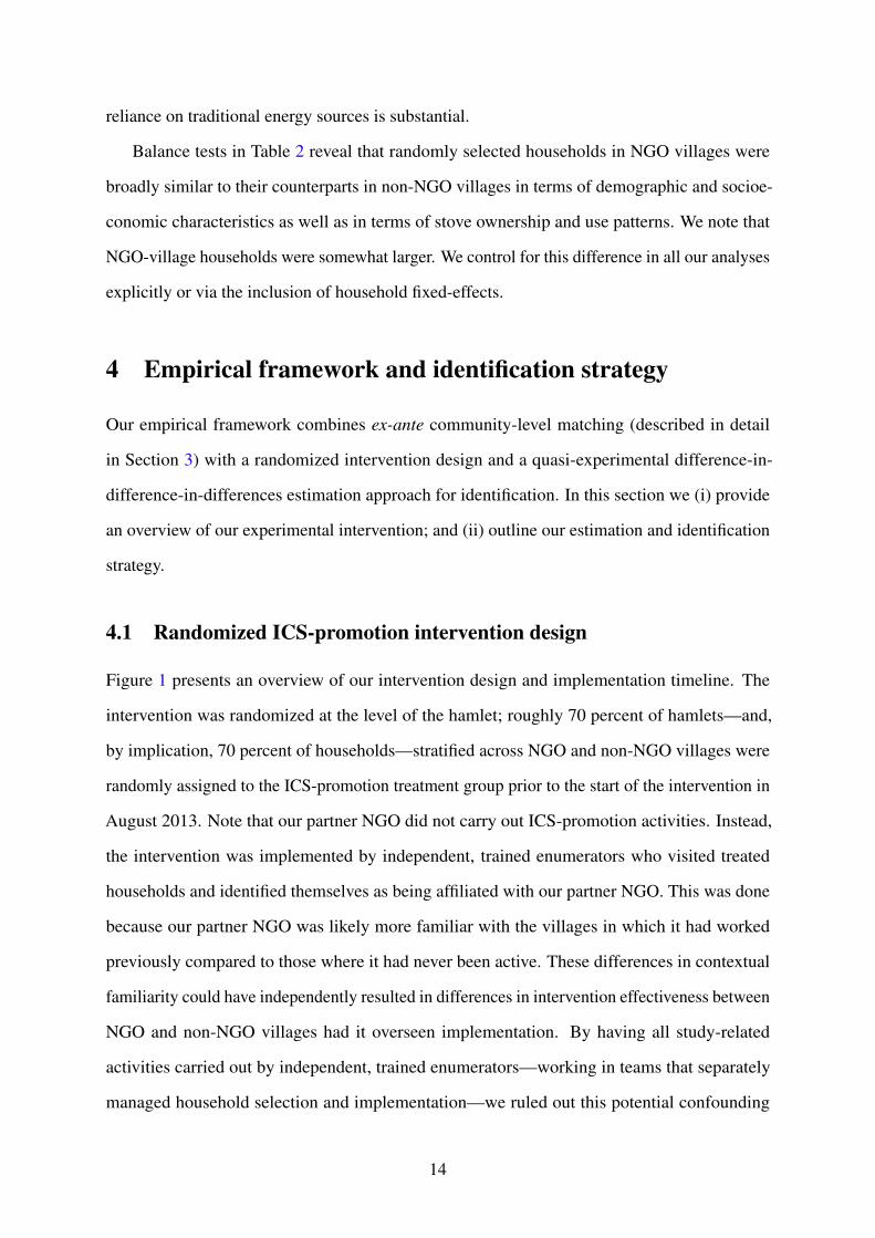
reliance on traditional energy sources is substantial.

Balance tests in Table 2 reveal that randomly selected households in NGO villages were

broadly similar to their counterparts in non-NGO villages in terms of demographic and socioe-

conomic characteristics as well as in terms of stove ownership and use patterns. We note that

NGO-village households were somewhat larger. We control for this difference in all our analyses

explicitly or via the inclusion of household fixed-effects.

4 Empirical framework and identification strategy

Our empirical framework combines ex-ante community-level matching (described in detail

in Section 3) with a randomized intervention design and a quasi-experimental difference-in-

difference-in-differences estimation approach for identification. In this section we (i) provide

an overview of our experimental intervention; and (ii) outline our estimation and identification

strategy.

4.1 Randomized ICS-promotion intervention design

Figure 1 presents an overview of our intervention design and implementation timeline. The

intervention was randomized at the level of the hamlet; roughly 70 percent of hamlets—and,

by implication, 70 percent of households—stratified across NGO and non-NGO villages were

randomly assigned to the ICS-promotion treatment group prior to the start of the intervention in

August 2013. Note that our partner NGO did not carry out ICS-promotion activities. Instead,

the intervention was implemented by independent, trained enumerators who visited treated

households and identified themselves as being affiliated with our partner NGO. This was done

because our partner NGO was likely more familiar with the villages in which it had worked

previously compared to those where it had never been active. These differences in contextual

familiarity could have independently resulted in differences in intervention effectiveness between

NGO and non-NGO villages had it overseen implementation. By having all study-related

activities carried out by independent, trained enumerators—working in teams that separately

managed household selection and implementation—we ruled out this potential confounding

14

channel.

Treated households received a personalized demonstration of two distinct ICS technologies:

an improved biomass cookstove, and an electric stove. At the end of the demonstration, survey

teams presented these households with an offer to purchase one or both of the stoves. This

offer consisted of a financial plan (the opportunity to make payments in three instalments)

combined with one of three randomized level of rebate (high, medium, or low—representing a

reduction in the cost of each stove by about 2, 20, and 30 percent, respectively).19 These rebates

were randomized at the household level and delivered as a discount counting against the final

instalment payment if a household was found to be still using the stove by that time. Households

in control hamlets did not receive the intervention; survey teams visited control households at

the same time as treated households to conduct follow-up surveys.

The stratified study design shown in Figure 1 enables us to compare the differential impact

of the same randomized intervention delivered by the same field team professing to be affiliated

with the same NGO across two institutionally distinct settings, namely, communities with which

the NGO had a preexisting relationship and those with which it did not. This allows us to isolate

how NGOs—and the trust and social capital they foster in their local communities—influences

the outcomes of interventions directly. Since our intervention is designed principally to increase

uptake of cleaner cooking technologies, our main outcome of interest is the purchase rate of

intervention ICS. To investigate heterogeneity in this rate across treated households located in

NGO and non-NGO villages separately, we estimate the following specification:

Yi jd = β1(T REAT MENT j

)+β2

(NGO j

)

+β3(T REAT MENT j ×NGO j

)+Xiδ+ γd + εi jd, (11)

where Yi jd is a binary variable that equals 1 if household i in hamlet j in district d purchased

at least one of the two intervention ICS offered during intervention activities and 0 if it did

not; T REAT MENT j is a binary variable that equals 1 if hamlet j is randomly assigned to the

treatment group and 0 if it is assigned to the control group; NGO j is a binary variable that equals

19The market price of the electric stove was around INR 1,000 (USD 20 in 2012) while that of the biomassstove was INR 1,400 (USD 28), approximately 17 and 24 percent of households’ reported monthly expenditure,respectively. The highest rebate amount, therefore, was around USD 6–8, depending on stove type.

15

1 if hamlet j is located in an NGO village and 0 if it is in a non-NGO village; Xi j is a matrix of

household-level controls; γd is a district fixed-effect; and εi j is a normally distributed error term.

Our coefficient of interest is β3, which sheds light on the additional impact of the randomized

ICS-promotion intervention on purchase rates in the NGO stratum of villages.

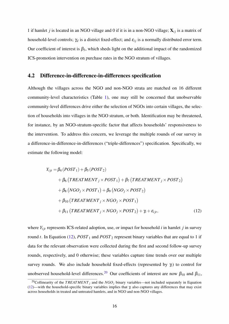
4.2 Difference-in-difference-in-differences specification

Although the villages across the NGO and non-NGO strata are matched on 16 different

community-level characteristics (Table 1), one may still be concerned that unobservable

community-level differences drive either the selection of NGOs into certain villages, the selec-

tion of households into villages in the NGO stratum, or both. Identification may be threatened,

for instance, by an NGO-stratum-specific factor that affects households’ responsiveness to

the intervention. To address this concern, we leverage the multiple rounds of our survey in

a difference-in-difference-in-differences (“triple-differences”) specification. Specifically, we

estimate the following model:

Yi jt =β4 (POST 1)+β5 (POST 2)

+β6(T REAT MENT j ×POST 1

)+β7

(T REAT MENT j ×POST 2

)

+β8(NGO j ×POST 1

)+β9

(NGO j ×POST 2

)

+β10(T REAT MENT j ×NGO j ×POST 1

)

+β11(T REAT MENT j ×NGO j ×POST 2

)+ γi + εi jt , (12)

where Yi jt represents ICS-related adoption, use, or impact for household i in hamlet j in survey

round t. In Equation (12), POST 1 and POST 2 represent binary variables that are equal to 1 if

data for the relevant observation were collected during the first and second follow-up survey

rounds, respectively, and 0 otherwise; these variables capture time trends over our multiple

survey rounds. We also include household fixed-effects (represented by γi) to control for

unobserved household-level differences.20 Our coefficients of interest are now β10 and β11,

20Collinearity of the T REAT MENT j and the NGO j binary variables—not included separately in Equation(12)—with the household-specific binary variables implies that γi also captures any differences that may existacross households in treated and untreated hamlets, and in NGO and non-NGO villages.

16

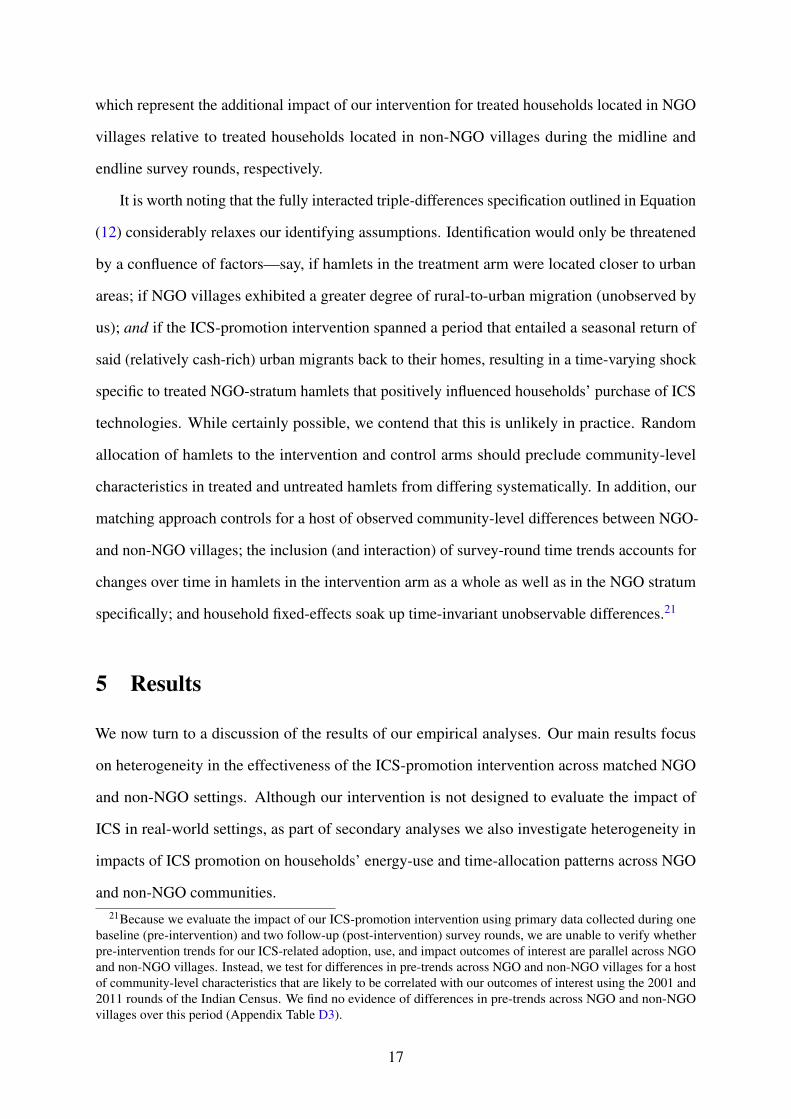
which represent the additional impact of our intervention for treated households located in NGO

villages relative to treated households located in non-NGO villages during the midline and

endline survey rounds, respectively.

It is worth noting that the fully interacted triple-differences specification outlined in Equation

(12) considerably relaxes our identifying assumptions. Identification would only be threatened

by a confluence of factors—say, if hamlets in the treatment arm were located closer to urban

areas; if NGO villages exhibited a greater degree of rural-to-urban migration (unobserved by

us); and if the ICS-promotion intervention spanned a period that entailed a seasonal return of

said (relatively cash-rich) urban migrants back to their homes, resulting in a time-varying shock

specific to treated NGO-stratum hamlets that positively influenced households’ purchase of ICS

technologies. While certainly possible, we contend that this is unlikely in practice. Random

allocation of hamlets to the intervention and control arms should preclude community-level

characteristics in treated and untreated hamlets from differing systematically. In addition, our

matching approach controls for a host of observed community-level differences between NGO-

and non-NGO villages; the inclusion (and interaction) of survey-round time trends accounts for

changes over time in hamlets in the intervention arm as a whole as well as in the NGO stratum

specifically; and household fixed-effects soak up time-invariant unobservable differences.21

5 Results

We now turn to a discussion of the results of our empirical analyses. Our main results focus

on heterogeneity in the effectiveness of the ICS-promotion intervention across matched NGO

and non-NGO settings. Although our intervention is not designed to evaluate the impact of

ICS in real-world settings, as part of secondary analyses we also investigate heterogeneity in

impacts of ICS promotion on households’ energy-use and time-allocation patterns across NGO

and non-NGO communities.21Because we evaluate the impact of our ICS-promotion intervention using primary data collected during one

baseline (pre-intervention) and two follow-up (post-intervention) survey rounds, we are unable to verify whetherpre-intervention trends for our ICS-related adoption, use, and impact outcomes of interest are parallel across NGOand non-NGO villages. Instead, we test for differences in pre-trends across NGO and non-NGO villages for a hostof community-level characteristics that are likely to be correlated with our outcomes of interest using the 2001 and2011 rounds of the Indian Census. We find no evidence of differences in pre-trends across NGO and non-NGOvillages over this period (Appendix Table D3).

17

5.1 Effectiveness of the intervention across NGO and non-NGO villages

5.1.1 Household-level purchase of intervention ICS technologies

Our primary outcome of interest is household-level purchase of ICS technologies promoted

during the ICS-promotion intervention. Figure 2 highlights the mean purchase rate for house-

holds located in treated hamlets in NGO and non-NGO villages. Nearly 60 percent of treated

households in NGO villages purchase at least one of the two intervention ICS. In non-NGO

villages, the corresponding figure is approximately 45 percent. We next evaluate this difference

more rigorously in a linear regression framework. Table 3 presents our results. We find that

the promotion campaign is extremely effective at encouraging the uptake of the intervention

stoves; as shown in column (1), over half of targeted households purchase at least one of the two

promoted ICS technologies. However, when we disaggregate our results by NGO and non-NGO

villages following Equation (11) in column (2), we find that the purchase rate is 14 percentage

points (31 percent) higher in treated hamlets located in NGO villages—a statistically significant

and positive “NGO effect.” These results are robust to the inclusion of household-level controls

that were found to be unbalanced at baseline in Table 2, as shown in column (3).

We check the robustness of these results in two ways. First, in Figure C2, we present results

from the application of an approach inspired by randomization-based inferential procedures

(Athey and Imbens, 2017) to village-level NGO stratum allocation. Our approach relies on

randomly assigning villages to placebo NGO and non-NGO strata, and re-estimating Equation

(11); this process is repeated 1,000 times to obtain a distribution of placebo “NGO effect”

estimates. If the effect we observe was due to the chance selection of the villages in our NGO

and non-NGO strata, we would expect to observe our actual estimate located near the middle of

this distribution. Instead, we find that only three percent of these placebo estimates are greater

than our actual estimates.

Next, in Appendix E, rather than characterizing NGO and non-NGO villages using a binary

variable, we characterize the village-specific “intensity” of NGO activity based on two different

measures: (i) the number of projects/initiatives the NGO has implemented in a particular village;

and (ii) the number of years it has been active in a particular village. We use these two measures

18

to separately re-estimate Equation (11) for heterogeneity in rates of ICS purchase and obtain

results that are consistent with our main findings.

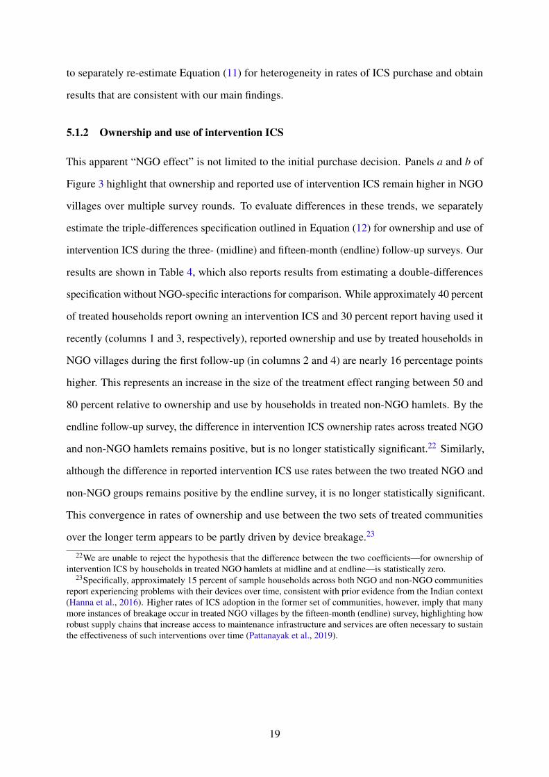
5.1.2 Ownership and use of intervention ICS

This apparent “NGO effect” is not limited to the initial purchase decision. Panels a and b of

Figure 3 highlight that ownership and reported use of intervention ICS remain higher in NGO

villages over multiple survey rounds. To evaluate differences in these trends, we separately

estimate the triple-differences specification outlined in Equation (12) for ownership and use of

intervention ICS during the three- (midline) and fifteen-month (endline) follow-up surveys. Our

results are shown in Table 4, which also reports results from estimating a double-differences

specification without NGO-specific interactions for comparison. While approximately 40 percent

of treated households report owning an intervention ICS and 30 percent report having used it

recently (columns 1 and 3, respectively), reported ownership and use by treated households in

NGO villages during the first follow-up (in columns 2 and 4) are nearly 16 percentage points

higher. This represents an increase in the size of the treatment effect ranging between 50 and

80 percent relative to ownership and use by households in treated non-NGO hamlets. By the

endline follow-up survey, the difference in intervention ICS ownership rates across treated NGO

and non-NGO hamlets remains positive, but is no longer statistically significant.22 Similarly,

although the difference in reported intervention ICS use rates between the two treated NGO and

non-NGO groups remains positive by the endline survey, it is no longer statistically significant.

This convergence in rates of ownership and use between the two sets of treated communities

over the longer term appears to be partly driven by device breakage.23

22We are unable to reject the hypothesis that the difference between the two coefficients—for ownership ofintervention ICS by households in treated NGO hamlets at midline and at endline—is statistically zero.

23Specifically, approximately 15 percent of sample households across both NGO and non-NGO communitiesreport experiencing problems with their devices over time, consistent with prior evidence from the Indian context(Hanna et al., 2016). Higher rates of ICS adoption in the former set of communities, however, imply that manymore instances of breakage occur in treated NGO villages by the fifteen-month (endline) survey, highlighting howrobust supply chains that increase access to maintenance infrastructure and services are often necessary to sustainthe effectiveness of such interventions over time (Pattanayak et al., 2019).

19

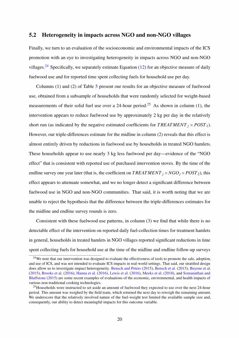
5.2 Heterogeneity in impacts across NGO and non-NGO villages

Finally, we turn to an evaluation of the socioeconomic and environmental impacts of the ICS

promotion with an eye to investigating heterogeneity in impacts across NGO and non-NGO

villages.24 Specifically, we separately estimate Equation (12) for an objective measure of daily

fuelwood use and for reported time spent collecting fuels for household use per day.

Columns (1) and (2) of Table 5 present our results for an objective measure of fuelwood

use, obtained from a subsample of households that were randomly selected for weight-based

measurements of their solid fuel use over a 24-hour period.25 As shown in column (1), the

intervention appears to reduce fuelwood use by approximately 2 kg per day in the relatively

short run (as indicated by the negative estimated coefficients for T REAT MENT j ×POST 1).

However, our triple-differences estimate for the midline in column (2) reveals that this effect is

almost entirely driven by reductions in fuelwood use by households in treated NGO hamlets.

These households appear to use nearly 3 kg less fuelwood per day—evidence of the “NGO

effect” that is consistent with reported use of purchased intervention stoves. By the time of the

endline survey one year later (that is, the coefficient on T REAT MENT j×NGO j×POST 2), this

effect appears to attenuate somewhat, and we no longer detect a significant difference between

fuelwood use in NGO and non-NGO communities. That said, it is worth noting that we are

unable to reject the hypothesis that the difference between the triple-differences estimates for

the midline and endline survey rounds is zero.

Consistent with these fuelwood use patterns, in column (3) we find that while there is no

detectable effect of the intervention on reported daily fuel-collection times for treatment hamlets

in general, households in treated hamlets in NGO villages reported significant reductions in time

spent collecting fuels for household use at the time of the midline and endline follow-up surveys

24We note that our intervention was designed to evaluate the effectiveness of tools to promote the sale, adoption,and use of ICS, and was not intended to evaluate ICS impacts in real-world settings. That said, our stratified designdoes allow us to investigate impact heterogeneity. Bensch and Peters (2015), Bensch et al. (2015), Beyene et al.(2015), Brooks et al. (2016), Hanna et al. (2016), Lewis et al. (2016), Meeks et al. (2018), and Somanathan andBluffstone (2015) are some recent examples of evaluations of the economic, environmental, and health impacts ofvarious non-traditional cooking technologies.

25Households were instructed to set aside an amount of fuelwood they expected to use over the next 24-hourperiod. This amount was weighed by the field team, which returned the next day to reweigh the remaining amount.We underscore that the relatively involved nature of the fuel-weight test limited the available sample size and,consequently, our ability to detect meaningful impacts for this outcome variable.

20

(column 4). This effect appears to be driven primarily by reductions in time spent collecting

fuelwood and other traditional fuels (Table D4). Once again, the two triple-differences estimates

are statistically indistinguishable from each other.

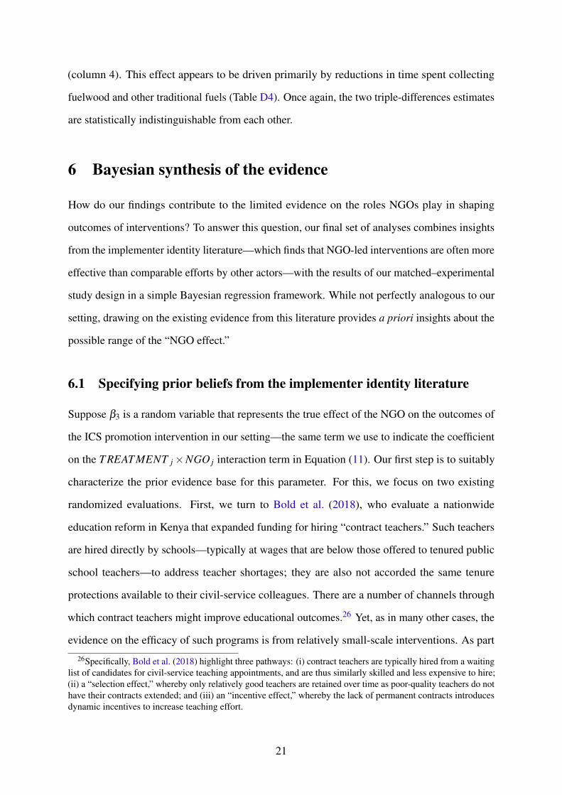
6 Bayesian synthesis of the evidence

How do our findings contribute to the limited evidence on the roles NGOs play in shaping

outcomes of interventions? To answer this question, our final set of analyses combines insights

from the implementer identity literature—which finds that NGO-led interventions are often more

effective than comparable efforts by other actors—with the results of our matched–experimental

study design in a simple Bayesian regression framework. While not perfectly analogous to our

setting, drawing on the existing evidence from this literature provides a priori insights about the

possible range of the “NGO effect.”

6.1 Specifying prior beliefs from the implementer identity literature

Suppose β3 is a random variable that represents the true effect of the NGO on the outcomes of

the ICS promotion intervention in our setting—the same term we use to indicate the coefficient

on the T REAT MENT j ×NGO j interaction term in Equation (11). Our first step is to suitably

characterize the prior evidence base for this parameter. For this, we focus on two existing

randomized evaluations. First, we turn to Bold et al. (2018), who evaluate a nationwide

education reform in Kenya that expanded funding for hiring “contract teachers.” Such teachers

are hired directly by schools—typically at wages that are below those offered to tenured public

school teachers—to address teacher shortages; they are also not accorded the same tenure

protections available to their civil-service colleagues. There are a number of channels through

which contract teachers might improve educational outcomes.26 Yet, as in many other cases, the

evidence on the efficacy of such programs is from relatively small-scale interventions. As part

26Specifically, Bold et al. (2018) highlight three pathways: (i) contract teachers are typically hired from a waitinglist of candidates for civil-service teaching appointments, and are thus similarly skilled and less expensive to hire;(ii) a “selection effect,” whereby only relatively good teachers are retained over time as poor-quality teachers do nothave their contracts extended; and (iii) an “incentive effect,” whereby the lack of permanent contracts introducesdynamic incentives to increase teaching effort.

21

of their large-scale evaluation, Bold et al. (2018) randomly assign a nationwide sample of public

schools to a control group, and one of two treatment groups that differ only in the identity of the

implementer—in one, the implementation is led by an NGO while in the other it is led by the

government. They find that “an additional contract teacher in a school where the program is

managed by the NGO increased test scores by roughly 0.18 standard deviations.” In contrast, the

treatment effect is both smaller and statistically insignificant in the government-implementation

schools. Digging deeper into mechanisms, they also find that contract teachers were actually

hired and in place for at least 12 percent more months in NGO-implementation schools over the

course of the intervention.

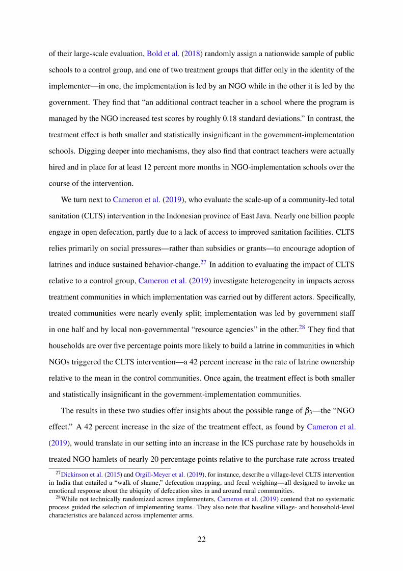
We turn next to Cameron et al. (2019), who evaluate the scale-up of a community-led total

sanitation (CLTS) intervention in the Indonesian province of East Java. Nearly one billion people

engage in open defecation, partly due to a lack of access to improved sanitation facilities. CLTS

relies primarily on social pressures—rather than subsidies or grants—to encourage adoption of

latrines and induce sustained behavior-change.27 In addition to evaluating the impact of CLTS

relative to a control group, Cameron et al. (2019) investigate heterogeneity in impacts across

treatment communities in which implementation was carried out by different actors. Specifically,

treated communities were nearly evenly split; implementation was led by government staff

in one half and by local non-governmental “resource agencies” in the other.28 They find that

households are over five percentage points more likely to build a latrine in communities in which

NGOs triggered the CLTS intervention—a 42 percent increase in the rate of latrine ownership

relative to the mean in the control communities. Once again, the treatment effect is both smaller

and statistically insignificant in the government-implementation communities.

The results in these two studies offer insights about the possible range of β3—the “NGO

effect.” A 42 percent increase in the size of the treatment effect, as found by Cameron et al.

(2019), would translate in our setting into an increase in the ICS purchase rate by households in

treated NGO hamlets of nearly 20 percentage points relative to the purchase rate across treated

27Dickinson et al. (2015) and Orgill-Meyer et al. (2019), for instance, describe a village-level CLTS interventionin India that entailed a “walk of shame,” defecation mapping, and fecal weighing—all designed to invoke anemotional response about the ubiquity of defecation sites in and around rural communities.

28While not technically randomized across implementers, Cameron et al. (2019) contend that no systematicprocess guided the selection of implementing teams. They also note that baseline village- and household-levelcharacteristics are balanced across implementer arms.

22

non-NGO hamlets. In contrast, the more conservative 12 percent estimate from Bold et al. (2018)

would imply a difference in the purchase rate between treated NGO and non-NGO hamlets of

closer to five percentage points. The midpoint of these two estimates is 12.5 percentage points.

This prior information suggests that we use a prior distribution f (β3) that assigns most of its

probability to the interval (0.05,0.20), and that the expected value of β3 under f (β3) be close

to 0.125. We, therefore, represent our prior information about β3 as follows:

β3 ∼ Beta(2,14) . (13)

The density of this prior distribution—a beta distribution with shape parameters α = 2 and

β = 14—is represented by the dashed line in panel a of Figure 4. The expected value of β3

under this prior is 0.125, and the most probable value is approximately 0.07, corresponding to

the peak in the density function. Just under two-thirds of the area under the curve lies between

0.05 and 0.20. Importantly, this distribution only has positive support over the interval [0,1].

Together, these characteristics implicitly capture the prior information that the “NGO effect” is

strictly positive but not excessively high.29

6.2 Results

With this prior specified, we fit a Bayesian multilevel mixed-effects model corresponding to

the specification outlined in Equation (11) to investigate heterogeneity in purchase rates across

treated NGO and non-NGO hamlets (described in detail in Appendix F).30 Broadly speaking, the

goal of this exercise is to understand how prior knowledge combined with observed data lead to

updated beliefs about parameters of interest. Our results are shown in panel a of Figure 4, where

29Admittedly, the choice of the specific beta prior outlined in Equation (13) is somewhat arbitrary as anynumber of alternative distributions would satisfy our outlined mean- and interval-related criteria. We note thatthe relative dearth of related evidence that we might draw upon to examine the distribution of estimates in moredetail contributes to this subjectivity. Given this constraint, we believe our specified prior distribution does areasonable job of characterizing the existing evidence. In addition, we also test the robustness of our results to priorspecification using both “weak” and “strong” prior distributional assumptions.

30Multilevel models account for hierarchical structures within the data. In our case, households are locatedwithin hamlets that are part of villages, which themselves are within districts. We specify a model that accounts foreach of these levels, allowing level-specific effects to also vary randomly based on specified prior distributions. Inaddition, we specify diffuse (“uninformative”) priors for all random model parameters besides our parameter ofinterest.

23

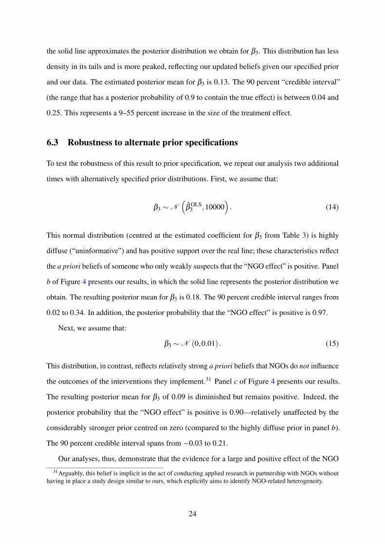
the solid line approximates the posterior distribution we obtain for β3. This distribution has less

density in its tails and is more peaked, reflecting our updated beliefs given our specified prior

and our data. The estimated posterior mean for β3 is 0.13. The 90 percent “credible interval”

(the range that has a posterior probability of 0.9 to contain the true effect) is between 0.04 and

0.25. This represents a 9–55 percent increase in the size of the treatment effect.

6.3 Robustness to alternate prior specifications

To test the robustness of this result to prior specification, we repeat our analysis two additional

times with alternatively specified prior distributions. First, we assume that:

β3 ∼ N

(

β̂ OLS3 ,10000

)

. (14)

This normal distribution (centred at the estimated coefficient for β3 from Table 3) is highly

diffuse (“uninformative”) and has positive support over the real line; these characteristics reflect

the a priori beliefs of someone who only weakly suspects that the “NGO effect” is positive. Panel

b of Figure 4 presents our results, in which the solid line represents the posterior distribution we

obtain. The resulting posterior mean for β3 is 0.18. The 90 percent credible interval ranges from

0.02 to 0.34. In addition, the posterior probability that the “NGO effect” is positive is 0.97.

Next, we assume that:

β3 ∼ N (0,0.01) . (15)

This distribution, in contrast, reflects relatively strong a priori beliefs that NGOs do not influence

the outcomes of the interventions they implement.31 Panel c of Figure 4 presents our results.

The resulting posterior mean for β3 of 0.09 is diminished but remains positive. Indeed, the

posterior probability that the “NGO effect” is positive is 0.90—relatively unaffected by the

considerably stronger prior centred on zero (compared to the highly diffuse prior in panel b).

The 90 percent credible interval spans from −0.03 to 0.21.

Our analyses, thus, demonstrate that the evidence for a large and positive effect of the NGO

31Arguably, this belief is implicit in the act of conducting applied research in partnership with NGOs withouthaving in place a study design similar to ours, which explicitly aims to identify NGO-related heterogeneity.

24

on the effectiveness of the ICS-promotion intervention is relatively robust—even under strong

prior distributional assumptions about the lack of such an effect. We also show how evidence

from related research can be used to inform these distributional assumptions and guide causal

inference.

7 Conclusion

Using data from an experimental intervention covering nearly 1,000 households across approxi-

mately 100 geographically distinct hamlets in rural Uttarakhand, India, we highlight how NGOs

directly influence the outcomes of applied interventions. We first develop a model of household

decision-making grounded in transaction costs. We posit that NGOs lower transaction costs,

and thus enhance the effectiveness of the interventions they implement. To empirically test

our model’s prediction, we use ex ante matching to create two observationally similar sub-

samples of villages that are differentiated only by prior exposure to a local development NGO.

In partnership with this NGO, we then implement a stratified, cluster randomized controlled

trial (RCT) designed to evaluate the effectiveness of an ICS-promotion campaign to identify

implementer-driven heterogeneity in technology adoption, use and impacts.

We uncover a large, positive, and statistically significant “NGO effect”—prior exposure

to the NGO increases the effectiveness of the intervention by nearly 30 percent. In line with

our model’s predictions, ICS purchase rates for households in treated hamlets located in “NGO

villages” are 14 percentage points (31 percent) higher than for households in treated hamlets

located in matched “non-NGO villages.” Using a difference-in-difference-in-differences (“triple-

differences”) specification that considerably relaxes our identifying assumptions and allows us

to identify the causal impact of an implementing NGO on the effectiveness of the intervention,

we find an even larger NGO effect on ICS ownership and use in these communities: households

in such communities are up to 16 percentage points more likely to have own and use an ICS,

representing a 50–80 percent increase in the size of the treatment effect. Consistent with these

patterns of ownership and use, households in villages with prior exposure to the NGO also

reduce daily fuelwood use and time spent collecting fuels. In contrast, we find no evidence

25

of any impact of the intervention on energy-use patterns for treated households in non-NGO

villages.

Although previous work has noted the presence of differential impacts across communities

with and without NGO activity, to the best of our knowledge, we are the first to rigorously

examine how the presence of an effective local NGO—and the specific institutional context

that represents—directly influences household decision-making and ultimately determines the

effectiveness of interventions. As such, our study begins to address a knowledge gap that

has significant implications for the policy relevance of experimental research conducted in

partnership with NGOs and other civil society organizations. Effective local organizations may

be crucial for the implementation of environmental, health, and development interventions in

remote, rural settings. Attempts to scale-up findings deemed effective in research partnerships

with such institutions, through national or regional policies, may prove much less successful

than anticipated if those partner institutions’ roles and contributions are insufficiently accounted

for. Alternatively, promoters of scaled-up interventions could achieve greater success if they

enlist the assistance of trusted local partners.

26

References

ALDASHEV, G., M. LIMARDI, AND T. VERDIER (2015): “Watchdogs of the Invisible Hand:NGO monitoring and industry equilibrium,” Journal of Development Economics, 116, 28–42.

ALDASHEV, G., M. MARINI, AND T. VERDIER (2014): “Brothers in alms? Coordinationbetween nonprofits on markets for donations,” Journal of Public Economics, 117, 182–200.

——— (2020): “Samaritan Bundles: Fundraising Competition and Inefficient Clustering inNGO Projects,” The Economic Journal, 130, 1541–1582.

ALDASHEV, G. AND C. NAVARRA (2018): “Development NGOs: Basic Facts,” Annals of

Public and Cooperative Economics, 89, 125–155.

ALLCOTT, H. (2015): “Site Selection Bias in Program Evaluation,” The Quarterly Journal of

Economics, 130, 1117–1165.

ANAND, U. (2015): “India has 31 lakh NGOs, more than double the number of schools,” The

Indian Express, retrieved from https://indianexpress.com/article/india/india-others/

india-has-31-lakh-ngos-twice-the-number-of-schools-almost-twice-number-of-policemen/

on July 11, 2017.

ATHEY, S. AND G. IMBENS (2017): “The Econometrics of Randomized Experiments,” inHandbook of Field Experiments, Elsevier, 73–140.

BAILIS, R., R. DRIGO, A. GHILARDI, AND O. MASERA (2015): “The carbon footprint oftraditional woodfuels,” Nature Climate Change, 5, 266–272.

BANERJEE, A., R. BANERJI, J. BERRY, E. DUFLO, H. KANNAN, S. MUKERJI, M. SHOT-LAND, AND M. WALTON (2017): “From Proof of Concept to Scalable Policies: Challengesand Solutions, with an Application,” Journal of Economic Perspectives, 31, 73–102.

BANERJEE, A., E. DUFLO, N. GOLDBERG, D. KARLAN, R. OSEI, W. PARIENTE, J. SHAPIRO,B. THUYSBAERT, AND C. UDRY (2015): “A multifaceted program causes lasting progressfor the very poor: Evidence from six countries,” Science, 348, 1260799.

BANERJEE, A. V., A. H. AMSDEN, R. H. BATES, J. N. BHAGWATI, A. DEATON, AND

N. STERN (2007): Making Aid Work, The MIT Press.

BARRETT, C. B. AND M. R. CARTER (2014): “A Retreat from Radical Skepticism: Rebalanc-ing Theory, Observational Data, and Randomization in Development Economics,” in Field

Experiments and Their Critics: Essays on the Uses and Abuses of Experimentation in the

Social Sciences, ed. by D. Teele, Yale University Press, 58–77.

BENGTSSON, N. (2013): “Catholics versus Protestants: On the Benefit Incidence of Faith-BasedForeign Aid,” Economic Development and Cultural Change, 61, 479–502.

BENSCH, G., M. GRIMM, AND J. PETERS (2015): “Why do households forego high returnsfrom technology adoption? Evidence from improved cooking stoves in Burkina Faso,” Journal

of Economic Behavior & Organization, 116, 187–205.

27

BENSCH, G. AND J. PETERS (2015): “The intensive margin of technology adoption – Experi-mental evidence on improved cooking stoves in rural Senegal,” Journal of Health Economics,42, 44–63.

BERGE, L. I. O., K. BJORVATN, K. S. JUNIWATY, AND B. TUNGODDEN (2012): “BusinessTraining in Tanzania: From Research-driven Experiment to Local Implementation,” Journal

of African Economies, 21, 808–827.

BERNARD, T., A. DE JANVRY, S. MBAYE, AND E. SADOULET (2017): “Expected ProductMarket Reforms and Technology Adoption by Senegalese Onion Producers,” American

Journal of Agricultural Economics, 99, 1096–1115.

BESLEY, T. AND M. GHATAK (2001): “Government Versus Private Ownership of PublicGoods,” The Quarterly Journal of Economics, 116, 1343–1372.

——— (2017): “Public–private partnerships for the provision of public goods: Theory and anapplication to NGOs,” Research in Economics, 71, 356–371.

BEYENE, A. D., R. A. BLUFFSTONE, S. DISSANAYAKE, Z. GEBREEGZIABHER, P. MAR-TINSSON, A. MEKONNEN, AND M. TOMAN (2015): “Can improved biomass cookstovescontribute to REDD+ in low-income countries? Evidence from a controlled cooking testtrial with randomized behavioral treatments,” World Bank Policy Research Working Paper№ 7394.

BOLD, T., M. KIMENYI, G. MWABU, A. NG’ANG’A, AND J. SANDEFUR (2018): “Experi-mental evidence on scaling up education reforms in Kenya,” Journal of Public Economics,168, 1–20.

BRASS, J. (2016): Allies or Adversaries: NGOs and the State in Africa, Cambridge UniversityPress.

BRASS, J. N. (2012): “Why Do NGOs Go Where They Go? Evidence from Kenya,” World

Development, 40, 387–401.

BRASS, J. N., W. LONGHOFER, R. S. ROBINSON, AND A. SCHNABLE (2018): “NGOs andinternational development: A review of thirty-five years of scholarship,” World Development,112, 136–149.

BROOKS, N., V. BHOJVAID, M. JEULAND, J. LEWIS, O. PATANGE, AND S. PATTANAYAK

(2016): “How much do alternative cookstoves reduce biomass fuel use? Evidence from NorthIndia,” Resource and Energy Economics, 43, 153–171.

CAMERON, L., S. OLIVIA, AND M. SHAH (2019): “Scaling up sanitation: Evidence from anRCT in Indonesia,” Journal of Development Economics, 138, 1–16.

CRUMP, R. K., V. J. HOTZ, G. W. IMBENS, AND O. A. MITNIK (2009): “Dealing with limitedoverlap in estimation of average treatment effects,” Biometrika, 96, 187–199.

DEATON, A. (2010): “Instruments, Randomization, and Learning about Development,” Journal

of Economic Literature, 48, 424–455.

DEVARAJAN, S., S. KHEMANI, AND M. WALTON (2013): “Can Civil Society OvercomeGovernment Failure in Africa?” The World Bank Research Observer, 29, 20–47.

28

DICKINSON, K. L., S. R. PATIL, S. K. PATTANAYAK, C. POULOS, AND J.-C. YANG (2015):“Nature’s Call: Impacts of Sanitation Choices in Orissa, India,” Economic Development and

Cultural Change, 64, 1–29.

EDLIN, A. S. AND C. SHANNON (1998): “Strict Monotonicity in Comparative Statics,” Journal

of Economic Theory, 81, 201–219.

FOSTER, A. D. AND M. R. ROSENZWEIG (2010): “Microeconomics of Technology Adoption,”Annual Review of Economics, 2, 395–424.

FRANCOIS, P. (2001): “Employee Care and the Role of Nonprofit Organizations,” Journal of

Institutional and Theoretical Economics, 157, 443.

——— (2003): “Not-for-Profit Provision of Public Services,” The Economic Journal, 113,C53–C61.

FRUTTERO, A. AND V. GAURI (2005): “The Strategic Choices of NGOs: Location Decisionsin Rural Bangladesh,” Journal of Development Studies, 41, 759–787.

GIBBONS, R. (2010): “Inside Organizations: Pricing, Politics, and Path Dependence,” Annual

Review of Economics, 2, 337–365.

GLENNERSTER, R. (2015): “A movement grows up. Running Randomized Evalua-tions: A Practical Guide.” Retrieved from http://runningres.com/blog/2015/7/13/

a-movement-grows-up on April 24, 2016.

GRANT, L. E. AND K. K. GROOMS (2017): “Do Nonprofits Encourage Environmental Compli-ance?” Journal of the Association of Environmental and Resource Economists, 4, S261–S288.

GROSSMAN, G., M. HUMPHREYS, AND G. SACRAMONE-LUTZ (2020): “Information Tech-nology and Political Engagement: Mixed Evidence from Uganda,” The Journal of Politics,82, 1321–1336.

GROSSMAN, M. (1972): “On the Concept of Health Capital and the Demand for Health,”Journal of Political Economy, 80, 223–255.

HANNA, R., E. DUFLO, AND M. GREENSTONE (2016): “Up in Smoke: The Influence ofHousehold Behavior on the Long-Run Impact of Improved Cooking Stoves,” American

Economic Journal: Economic Policy, 8, 80–114.

HENDERSON, J. V. AND Y. S. LEE (2015): “Organization of Disaster Aid Delivery: SpendingYour Donations,” Economic Development and Cultural Change, 63, 617–664.

HERMAN, M. L., G. L. HEAD, T. E. FOGARTY, AND P. M. JACKSON (2004): “Reputationand Mission Risks,” in Managing Risk in Nonprofit Organizations: A Comprehensive Guide,Wiley, 133–148.

HOLLOWAY, G., C. NICHOLSON, C. DELGADO, S. STAAL, AND S. EHUI (2000): “Agroindus-trialization through institutional innovation Transaction costs, cooperatives and milk-marketdevelopment in the east-African highlands,” Agricultural Economics, 23, 279–288.

ITO, T. (2009): “Caste discrimination and transaction costs in the labor market: Evidence fromrural North India,” Journal of Development Economics, 88, 292–300.

29

JACK, W. AND T. SURI (2014): “Risk Sharing and Transactions Costs: Evidence from Kenya'sMobile Money Revolution,” American Economic Review, 104, 183–223.

JAYACHANDRAN, S., J. DE LAAT, E. F. LAMBIN, C. Y. STANTON, R. AUDY, AND N. E.THOMAS (2017): “Cash for carbon: A randomized trial of payments for ecosystem servicesto reduce deforestation,” Science, 357, 267–273.

JEULAND, M. A. AND S. K. PATTANAYAK (2012): “Benefits and Costs of Improved Cook-stoves: Assessing the Implications of Variability in Health, Forest and Climate Impacts,”PLoS ONE, 7, e30338.

JEULAND, M. A., S. K. PATTANAYAK, AND R. BLUFFSTONE (2015): “The Economics ofHousehold Air Pollution,” Annual Review of Resource Economics, 7, 81–108.

JEULAND, M. A., S. K. PATTANAYAK, S. SAMADDAR, R. SHAH, AND M. VORA (2020):“Adoption and impacts of improved biomass cookstoves in rural Rajasthan,” Energy for

Sustainable Development, 57, 149–159.

JOHNSON-LANS, S. (2008): “Do NGOs make a difference: A case study of rural Rajasthan,”Vassar College Faculty Research and Reports № 4.

JONES, D., D. MOLITOR, AND J. REIF (2019): “What do Workplace Wellness Programs do?Evidence from the Illinois Workplace Wellness Study,” The Quarterly Journal of Economics,134, 1747–1791.

KING, G., E. GAKIDOU, N. RAVISHANKAR, R. T. MOORE, J. LAKIN, M. VARGAS, M. M.TÉLLEZ-ROJO, J. E. H. ÁVILA, M. H. ÁVILA, AND H. H. LLAMAS (2007): “A “politicallyrobust” experimental design for public policy evaluation, with application to the MexicanUniversal Health Insurance program,” Journal of Policy Analysis and Management, 26,479–506.

KRANTON, R. E. (1996): “Reciprocal Exchange: A Self-Sustaining System,” American Eco-

nomic Review, 86, 830–851.

LEWIS, J. J., J. W. HOLLINGSWORTH, R. T. CHARTIER, E. M. COOPER, W. M. FOSTER,G. L. GOMES, P. S. KUSSIN, J. J. MACINNIS, B. K. PADHI, P. PANIGRAHI, C. E. RODES,I. T. RYDE, A. K. SINGHA, H. M. STAPLETON, J. THORNBURG, C. J. YOUNG, J. N.MEYER, AND S. K. PATTANAYAK (2016): “Biogas Stoves Reduce Firewood Use, HouseholdAir Pollution, and Hospital Visits in Odisha, India,” Environmental Science & Technology, 51,560–569.

LEWIS, J. J. AND S. K. PATTANAYAK (2012): “Who Adopts Improved Fuels and Cookstoves?A Systematic Review,” Environmental Health Perspectives, 120, 637–645.

LIN, L., S. K. PATTANAYAK, E. O. SILLS, AND W. D. SUNDERLIN (2012): “Site selection forforest carbon projects,” in Analysing REDD+: Challenges and choices, ed. by A. Angelsen,M. Brockhaus, W. D. Sunderlin, and L. Verchot, Bogor, Indonesia: Center for InternationalForestry Research (CIFOR), chap. 12, 209–230.

MACLEAN, L. M., J. N. BRASS, S. CARLEY, A. EL-ARINI, AND S. BREEN (2015): “Democ-racy and the Distribution of NGOs Promoting Renewable Energy in Africa,” Journal of

Development Studies, 51, 725–742.

30

MAURYA, N. K. (2014): “A Critical Evaluation of the State Finances of the UttarakhandGovernments: 2002-03 to 2011-12,” Tech. rep., Fourteenth Finance Commission, Governmentof India.

MEEKS, R., K. R. E. SIMS, AND H. THOMPSON (2018): “Waste Not: Can Household BiogasDeliver Sustainable Development?” Environmental and Resource Economics, 72, 763–794.

MICKLEWRIGHT, J. AND A. WRIGHT (2003): “Private Donations for International Develop-ment,” WIDER Discussion Paper № 2003/82.

MIGUEL, E. AND M. KREMER (2004): “Worms: Identifying Impacts on Education and Healthin the Presence of Treatment Externalities,” Econometrica, 72, 159–217.

MOBARAK, A. M., P. DWIVEDI, R. BAILIS, L. HILDEMANN, AND G. MILLER (2012): “Lowdemand for nontraditional cookstove technologies,” Proceedings of the National Academy of

Sciences, 109, 10815–10820.

NIEHAUS, P. AND S. SUKHTANKAR (2013): “The marginal rate of corruption in publicprograms: Evidence from India,” Journal of Public Economics, 104, 52–64.

ORGILL-MEYER, J., S. K. PATTANAYAK, N. CHINDARKAR, K. L. DICKINSON, U. PANDA,S. RAI, B. SAHOO, A. SINGHA, AND M. A. JEULAND (2019): “Long-term impact ofa community-led sanitation campaign in India, 2005–2016,” Bulletin of the World Health

Organization, 97, 523–533A.

PATTANAYAK, S. K., M. A. JEULAND, J. J. LEWIS, F. USMANI, N. BROOKS, V. BHOJVAID,A. KAR, L. LIPINSKI, L. MORRISON, O. PATANGE, N. RAMANATHAN, I. H. REHMAN,R. THADANI, M. VORA, AND V. RAMANATHAN (2019): “Experimental evidence on promo-tion of electric and improved biomass cookstoves,” Proceedings of the National Academy of

Sciences, 116, 13282–13287.

PATTANAYAK, S. K., R. A. KRAMER, AND J. R. VINCENT (2017): “Ecosystem change andhuman health: implementation economics and policy,” Philosophical Transactions of the

Royal Society B: Biological Sciences, 372, 20160130.

PATTANAYAK, S. K. AND A. PFAFF (2009): “Behavior, Environment, and Health in DevelopingCountries: Evaluation and Valuation,” Annual Review of Resource Economics, 1, 183–217.

PATTANAYAK, S. K., J.-C. YANG, K. L. DICKINSON, C. POULOS, S. R. PATIL, R. K.MALLICK, J. L. BLITSTEIN, AND P. PRAHARAJ (2009): “Shame or subsidy revisited: socialmobilization for sanitation in Orissa, India,” Bulletin of the World Health Organization, 87,580–587.

PETERS, J., J. LANGBEIN, AND G. ROBERTS (2018): “Generalization in the Tropics – De-velopment Policy, Randomized Controlled Trials, and External Validity,” The World Bank

Research Observer, 33, 34–64.

RAVALLION, M. (2009): “Evaluation in the Practice of Development,” The World Bank Research

Observer, 24, 29–53.

ROSENBAUM, P. R. AND D. B. RUBIN (1984): “Reducing Bias in Observational Studies UsingSubclassification on the Propensity Score,” Journal of the American Statistical Association,79, 516–524.

31

ROSENTHAL, J., K. BALAKRISHNAN, N. BRUCE, D. CHAMBERS, J. GRAHAM, D. JACK,L. KLINE, O. MASERA, S. MEHTA, I. R. MERCADO, G. NETA, S. PATTANAYAK,E. PUZZOLO, H. PETACH, A. PUNTURIERI, A. RUBINSTEIN, M. SAGE, R. STURKE,A. SHANKAR, K. SHERR, K. SMITH, AND G. YADAMA (2017): “Implementation Scienceto Accelerate Clean Cooking for Public Health,” Environmental Health Perspectives, 125.

SHARMA, B. P., S. K. PATTANAYAK, M. NEPAL, P. SHYAMSUNDAR, AND B. S. KARKY

(2015): “REDD+ Impacts: Evidence from Nepal,” South Asian Network for Developmentand Environmental Economics (SANDEE) Working Paper № 95-15.

SOMANATHAN, E. AND R. BLUFFSTONE (2015): “Biogas: Clean Energy Access with Low-Cost Mitigation of Climate Change,” Environmental and Resource Economics, 62, 265–277.

SURI, T. (2011): “Selection and Comparative Advantage in Technology Adoption,” Economet-

rica, 79, 159–209.

VENKATARAMAN, C. (2005): “Residential Biofuels in South Asia: Carbonaceous AerosolEmissions and Climate Impacts,” Science, 307, 1454–1456.

VIVALT, E. (2020): “How Much Can We Generalize From Impact Evaluations?” Journal of the

European Economic Association, 18, 3045–3089.

WERKER, E. AND F. Z. AHMED (2008): “What Do Nongovernmental Organizations Do?”Journal of Economic Perspectives, 22, 73–92.

WESTFALL, P. H. AND S. S. YOUNG (1993): Resampling-Based Multiple Testing: Examples

and Methods for p-Value Adjustment, Wiley-Interscience.

WOOLCOCK, M., S. SZRETER, AND V. RAO (2011): “How and Why Does History Matter forDevelopment Policy?” Journal of Development Studies, 47, 70–96.

32

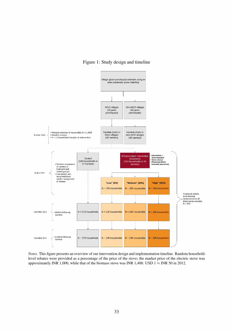
Figure 1: Study design and timeline

Notes. This figure presents an overview of our intervention design and implementation timeline. Random household-level rebates were provided as a percentage of the price of the stove; the market price of the electric stove wasapproximately INR 1,000, while that of the biomass stove was INR 1,400. USD 1 ≈ INR 50 in 2012.

33

Figure 2: Mean intervention ICS purchase rates in treated hamlets in NGO and non-NGOvillages

Notes. This figure plots the share of households in NGO and non-NGO villages that purchased at least oneintervention ICS in response to the ICS-promotion intervention as a percentage of all treated households in therespective stratum. Error bars represent 95 percent confidence intervals for the means.

34

Figure 3: ICS ownership and use in NGO and non-NGO villages

Notes. Panels a and c plot the share of households that own at least one of the two intervention ICS or an improvedICS, respectively, as a percentage of all (treated and untreated) sample households in the indicated stratum ofvillages. Panels b and d plot the subset of these households that report having used these devices in the weekprior to the survey as a percentage of all (treated and untreated) sample households in the indicated stratum ofvillages. “Improved stove” includes stoves fueled by biogas, electricity, LPG, kerosene, and commercially availableefficient biomass cookstoves; we also include the two ICS promoted as part of the promotion intervention in thisdefinition. Error bars represent 95 percent confidence intervals for the means. Baseline survey activities occurredapproximately one year before the intervention; midline and endline surveys occurred approximately three andfifteen months, respectively, after the intervention (see Figure 1).

35

Figure 4: Bayesian analysis of heterogeneity in ICS purchase across NGO and non-NGO hamlets

Notes. This figure plots prior and posterior distributions of the β3 parameter, which represents the additional effectof the ICS promotion intervention on purchase rates in treated NGO hamlets relative to treated non-NGO hamlets.Posterior distributions are estimated via Markov Chain Monte Carlo (MCMC) simulation. Specifically, we ran50,000 MCMC samples after a burn-in period of 10,000 iterations, with thinning every fifth iteration. In panel a,f (β3) = Beta(2,14); in panel b, f (β3) = N (0,10000); and in panel c, f (β3) = N (0,0.01). Diffuse priors areused for all other parameters in the underlying model for each panel (see Appendix F).

36

Table 1: Post-match balance on village-level characteristics across NGO and non-NGO villages

Village-level characteristic(1) (2) (3) (4)

NGO villages Non-NGO villagesMean Normalized

Mean/SD Mean/SD difference difference

Area (km2) 146.68 174.97 −28.29 −0.14[94.51] [268.64]

Total population 386.84 376.68 10.16 0.08[136.56] [130.02]

Scheduled Caste population share 0.26 0.28 −0.01 −0.04[0.29] [0.30]

Scheduled Tribe population share 0.01 0.00 0.01 0.31[0.03] [0.00]

Number of primary schools 1.11 1.05 0.05 0.15[0.46] [0.23]

Number of middle schools 0.37 0.32 0.05 0.11[0.50] [0.48]

Number of health centers 0.00 0.00 N/A N/A[0.00] [0.00]

Number of primary health centers 0.00 0.00 N/A N/A[0.00] [0.00]

Number of telephone connections 0.26 0.42 −0.16 −0.30[0.56] [0.51]

✶(Bus services) 0.11 0.05 0.05 0.19[0.32] [0.23]

✶(Credit societies) 0.00 0.00 N/A N/A[0.00] [0.00]

✶(Approach to village: paved road) 0.21 0.16 0.05 0.13[0.42] [0.37]

Distance from nearest town (km) 25.11 19.95 5.16 0.36[16.07] [11.86]

Forest area (hectares) 34.08 25.98 8.10 0.14[63.95] [51.82]

✶(Tap water) 0.89 1.00 −0.11 −0.47[0.32] [0.00]

✶(Electricity for all purposes) 0.05 0.00 0.05 0.32[0.23] [0.00]

N 19 19 38

Notes. Columns (1) and (2) show means and standard deviations (in brackets) for NGO and non-NGO villages, respectively,

for each of the village-level variables from the 2001 round of the Indian Census used for our final propensity score matching

exercise; column (3) shows the difference between the means in columns (1) and (2); and column (4) shows the normalized

difference between the means in columns (1) and (2). The Scheduled Castes and Scheduled Tribes are various historically

disadvantaged or indigenous groups in India that have received official recognition as such from the Indian government. t-tests

to check for statistical differences in means account for district fixed-effects. ∗ p < 0.10, ∗∗ p < 0.05, ∗∗∗ p < 0.01.

37

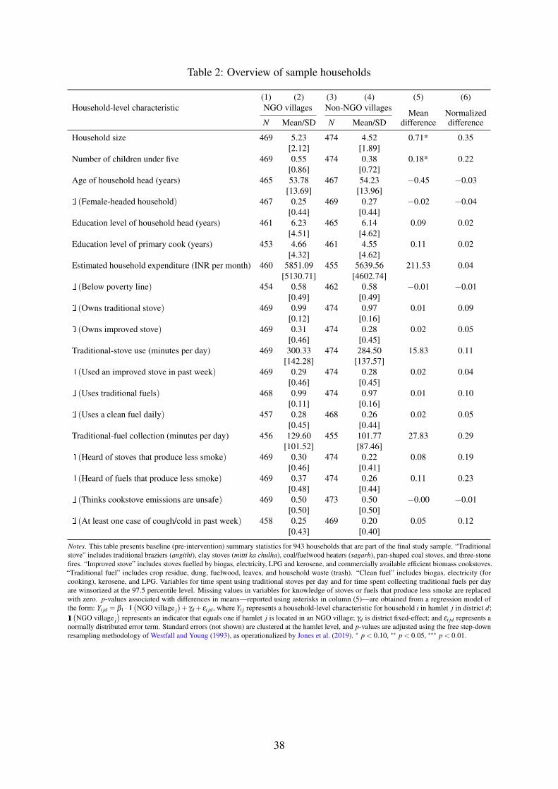
Table 2: Overview of sample households

Household-level characteristic(1) (2) (3) (4) (5) (6)NGO villages Non-NGO villages

Mean NormalizedN Mean/SD N Mean/SD difference difference

Household size 469 5.23 474 4.52 0.71* 0.35[2.12] [1.89]

Number of children under five 469 0.55 474 0.38 0.18* 0.22[0.86] [0.72]

Age of household head (years) 465 53.78 467 54.23 −0.45 −0.03[13.69] [13.96]

✶(Female-headed household) 467 0.25 469 0.27 −0.02 −0.04[0.44] [0.44]

Education level of household head (years) 461 6.23 465 6.14 0.09 0.02[4.51] [4.62]

Education level of primary cook (years) 453 4.66 461 4.55 0.11 0.02[4.32] [4.62]

Estimated household expenditure (INR per month) 460 5851.09 455 5639.56 211.53 0.04[5130.71] [4602.74]

✶(Below poverty line) 454 0.58 462 0.58 −0.01 −0.01[0.49] [0.49]

✶(Owns traditional stove) 469 0.99 474 0.97 0.01 0.09[0.12] [0.16]

✶(Owns improved stove) 469 0.31 474 0.28 0.02 0.05[0.46] [0.45]

Traditional-stove use (minutes per day) 469 300.33 474 284.50 15.83 0.11[142.28] [137.57]

✶(Used an improved stove in past week) 469 0.29 474 0.28 0.02 0.04[0.46] [0.45]

✶(Uses traditional fuels) 468 0.99 474 0.97 0.01 0.10[0.11] [0.16]

✶(Uses a clean fuel daily) 457 0.28 468 0.26 0.02 0.05[0.45] [0.44]

Traditional-fuel collection (minutes per day) 456 129.60 455 101.77 27.83 0.29[101.52] [87.46]

✶(Heard of stoves that produce less smoke) 469 0.30 474 0.22 0.08 0.19[0.46] [0.41]

✶(Heard of fuels that produce less smoke) 469 0.37 474 0.26 0.11 0.23[0.48] [0.44]

✶(Thinks cookstove emissions are unsafe) 469 0.50 473 0.50 −0.00 −0.01[0.50] [0.50]

✶(At least one case of cough/cold in past week) 458 0.25 469 0.20 0.05 0.12[0.43] [0.40]

Notes. This table presents baseline (pre-intervention) summary statistics for 943 households that are part of the final study sample. “Traditionalstove” includes traditional braziers (angithi), clay stoves (mitti ka chulha), coal/fuelwood heaters (sagarh), pan-shaped coal stoves, and three-stonefires. “Improved stove” includes stoves fuelled by biogas, electricity, LPG and kerosene, and commercially available efficient biomass cookstoves.“Traditional fuel” includes crop residue, dung, fuelwood, leaves, and household waste (trash). “Clean fuel” includes biogas, electricity (forcooking), kerosene, and LPG. Variables for time spent using traditional stoves per day and for time spent collecting traditional fuels per dayare winsorized at the 97.5 percentile level. Missing values in variables for knowledge of stoves or fuels that produce less smoke are replacedwith zero. p-values associated with differences in means—reported using asterisks in column (5)—are obtained from a regression model ofthe form: Yi jd = β1 ·✶

(NGO village j

)+ γd + εi jd , where Yi j represents a household-level characteristic for household i in hamlet j in district d;

✶(NGO village j

)represents an indicator that equals one if hamlet j is located in an NGO village; γd is district fixed-effect; and εi jd represents a

normally distributed error term. Standard errors (not shown) are clustered at the hamlet level, and p-values are adjusted using the free step-downresampling methodology of Westfall and Young (1993), as operationalized by Jones et al. (2019). ∗ p < 0.10, ∗∗ p < 0.05, ∗∗∗ p < 0.01.

38

Table 3: Effect of promotion on intervention ICS purchase in matched NGO/non-NGO villages

(1) (2) (3)

✶(Purchased intervention ICS)

T REAT MENT j 0.52*** 0.45*** 0.45***(0.03) (0.05) (0.05)

NGO j −0.03 −0.04(0.03) (0.03)

T REAT MENT j ×NGO j 0.14** 0.14**(0.06) (0.06)

Control mean 0 0 0District fixed-effects Yes Yes YesHousehold-level controls No No YesN 943 943 943Adjusted R2 0.24 0.24 0.24

Notes. The outcome variable is an indicator that equals 1 if household i inhamlet j purchased at least one of the two ICS promoted during the inter-vention. Column (1) presents aggregated results; results are disaggregatedby NGO and non-NGO villages (as shown in Equation 11) in columns (2)and (3). Baseline household-level controls for household size and num-ber of children under five are included in column (3). Standard errors (inparentheses) are clustered at the hamlet level. ∗ p < 0.10, ∗∗ p < 0.05, ∗∗∗

p < 0.01.

39

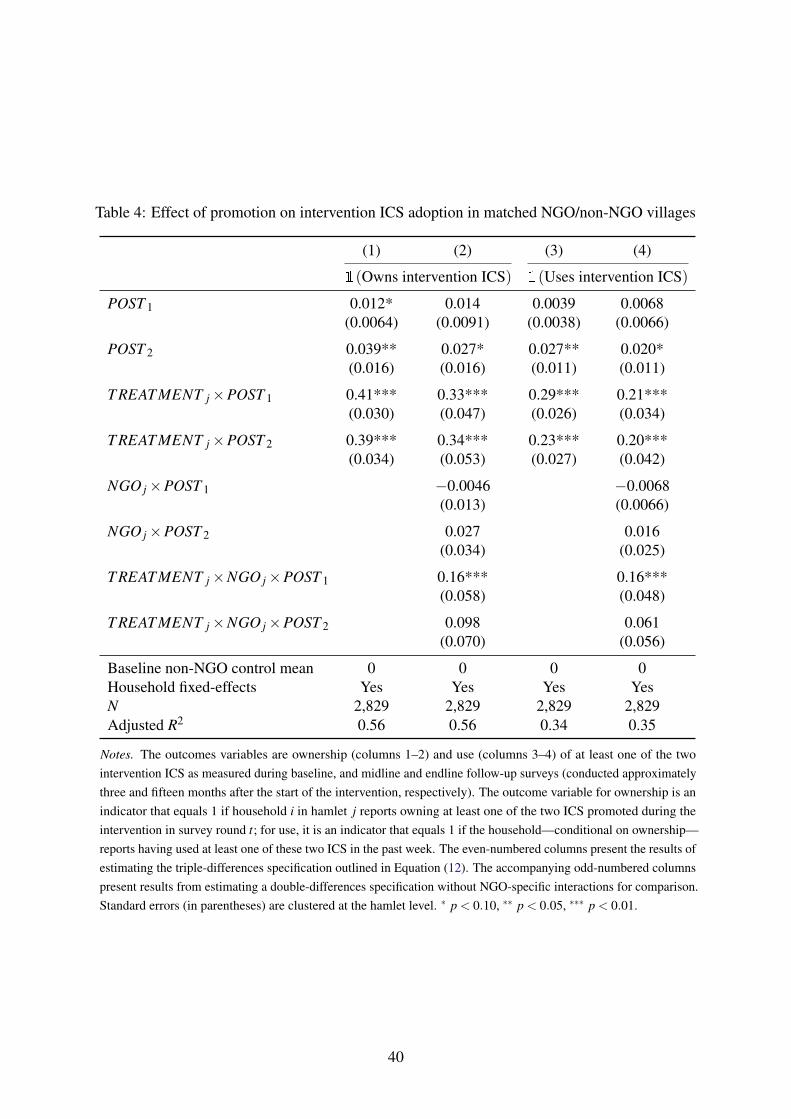
Table 4: Effect of promotion on intervention ICS adoption in matched NGO/non-NGO villages

(1) (2) (3) (4)

✶(Owns intervention ICS) ✶(Uses intervention ICS)

POST 1 0.012* 0.014 0.0039 0.0068(0.0064) (0.0091) (0.0038) (0.0066)

POST 2 0.039** 0.027* 0.027** 0.020*(0.016) (0.016) (0.011) (0.011)

T REAT MENT j ×POST 1 0.41*** 0.33*** 0.29*** 0.21***(0.030) (0.047) (0.026) (0.034)

T REAT MENT j ×POST 2 0.39*** 0.34*** 0.23*** 0.20***(0.034) (0.053) (0.027) (0.042)

NGO j ×POST 1 −0.0046 −0.0068(0.013) (0.0066)

NGO j ×POST 2 0.027 0.016(0.034) (0.025)

T REAT MENT j ×NGO j ×POST 1 0.16*** 0.16***(0.058) (0.048)

T REAT MENT j ×NGO j ×POST 2 0.098 0.061(0.070) (0.056)

Baseline non-NGO control mean 0 0 0 0Household fixed-effects Yes Yes Yes YesN 2,829 2,829 2,829 2,829Adjusted R2 0.56 0.56 0.34 0.35

Notes. The outcomes variables are ownership (columns 1–2) and use (columns 3–4) of at least one of the two

intervention ICS as measured during baseline, and midline and endline follow-up surveys (conducted approximately

three and fifteen months after the start of the intervention, respectively). The outcome variable for ownership is an

indicator that equals 1 if household i in hamlet j reports owning at least one of the two ICS promoted during the

intervention in survey round t; for use, it is an indicator that equals 1 if the household—conditional on ownership—

reports having used at least one of these two ICS in the past week. The even-numbered columns present the results of

estimating the triple-differences specification outlined in Equation (12). The accompanying odd-numbered columns

present results from estimating a double-differences specification without NGO-specific interactions for comparison.

Standard errors (in parentheses) are clustered at the hamlet level. ∗ p < 0.10, ∗∗ p < 0.05, ∗∗∗ p < 0.01.

40

Table 5: Impact of promotion on fuel collection and use in matched NGO/non-NGO villages

(1) (2) (3) (4)

Fuelwood use Fuel-collection time(kilograms per day) (minutes per day)

POST 1 4.42*** 3.38*** 3.96 −19.0(0.68) (0.57) (18.4) (18.5)

POST 2 1.50** 1.44 −9.83 −30.7**(0.75) (1.18) (15.5) (12.5)

T REAT MENT j ×POST 1 −2.01** −0.61 −25.6 19.2(0.93) (0.91) (21.9) (25.4)

T REAT MENT j ×POST 2 0.65 0.47 −14.0 12.8(1.08) (1.54) (17.0) (15.9)

NGO j ×POST 1 2.24** 53.3(1.12) (33.2)

NGO j ×POST 2 0.12 48.5*(1.47) (29.0)

T REAT MENT j ×NGO j ×POST 1 −2.93* −95.1**(1.67) (40.5)

T REAT MENT j ×NGO j ×POST 2 0.34 −60.0*(2.12) (32.2)

Baseline non-NGO control mean 8.9 8.9 114 114Household fixed-effects Yes Yes Yes YesN 1,143 1,143 2,829 2,829Adjusted R2 0.19 0.20 0.010 0.028

Notes. The outcome variables are daily fuelwood use (columns 1–2) and total time spent collecting

fuels (columns 3–4) as measured during baseline, and midline and endline follow-up surveys (con-

ducted approximately three and fifteen months after the start of the intervention, respectively). Daily

fuelwood use is derived from a 24-hour before–after household-level fuel-weighing test; we restrict

the analysis in columns (1) and (2) to the subsample of households that participated in such tests in

at least two of our three survey rounds (N = 388). The outcome variable for fuel-collection time is

derived from self-reported data on time spent (per day, week, or month) collecting fuelwood, crop

residue, leaves, dung, biomass pellets, kerosene, LPG, biogas, and—if relevant—any other fuel used

by the household; missing observations for time spent collecting fuel for up to six households in each

survey round are replaced with the survey-round-specific sample mean value. The even-numbered

columns present the results of estimating the triple-differences specification outlined in Equation

(12). The accompanying odd-numbered columns present results from estimating a double-differences

specification without NGO-specific interactions for comparison. Standard errors (in parentheses) are

clustered at the hamlet level. ∗ p < 0.10, ∗∗ p < 0.05, ∗∗∗ p < 0.01.

41

Online appendix to “NGOs and the effectiveness ofinterventions”

FARAZ USMANI†

MathematicaMARC JEULAND‡

Duke UniversitySUBHRENDU K. PATTANAYAK§

Duke University

†Research Economist, International Unit, Mathematica. fusmani@mathematica-mpr.com.‡Associate Professor, Sanford School of Public Policy and Duke Global Health Institute, Duke University.

Fellow, RWI–Leibniz Institute for Economic Research. marc.jeuland@duke.edu.§Oak Foundation Professor of Environmental and Energy Policy, Sanford School of Public Policy, Duke

University. subhrendu.pattanayak@duke.edu.

42

Appendix A The household’s optimization problem

The Lagrangian associated with the household’s optimization problem outlined in Section 2 isas follows:

maxa,l,c,t,m,k

L =u [c, l,a,s(e) ,e(a)]+λ [y− c− p(ξ ) ·m− r (ξ ) · k+w(T − s(e)− l − t (ξ ))]

+µ [T − l − s(e)− t (ξ )] . (A.1)

The first-order conditions associated with Equation (A.1) are as follows:

La = ua +usseea +ueea −λ[p(ξ ) ·am + r (ξ ) ·ak +w

(at(ξ )+ seea

)]−µ

[at(ξ )+ seea

]= 0(A.2)

Ll = ul −λ ·w−µ = 0 (A.3)

Lc = uc −λ = 0 (A.4)

Lt = uaat(ξ )+usseeaat(ξ )+ueeaat(ξ )−λw(1+ seeaat(ξ )

)−µ = 0 (A.5)

Lm = uaam +usseeaam +ueeaam −λ (p(ξ )+wseeaam)−µ = 0 (A.6)

Lk = uaak +usseeaak +ueeaak −λ (r (ξ )+wseeaak)−µ = 0 (A.7)

Lλ = y− c− pm− rk+w(T − s(e)− l − t (ξ )) = 0 (A.8)

Lµ = T − l − s(e)− t ≥ 0; µ (T − l − s(e)− t (ξ )) = 0. (A.9)

Assuming that all individuals work some non-zero hours, it follows from Equation (A.9) thatµ = 0. Then, from Equation (A.2), the optimal level of technology adoption (a∗) must fulfill

ua +usseea +ueea

λ−wseea

︸ ︷︷ ︸

Marginal benefit, MB(a)

= p(ξ ) ·am + r (ξ ) ·ak +wat(ξ )︸ ︷︷ ︸

Marginal cost, MC(a,ξ )

. (A.10)

43

Appendix B Elicitation/construction of variables

In this appendix, we describe how each of the variables we present in this study are elicited orconstructed from data collected during various rounds of survey activities (Figure 1). Englishtranslations of relevant extracts from survey instruments are included where appropriate.

B.1 Household-level stove- and fuel-use characteristics

Stove- and fuel-use characteristics are primarily constructed from data collected as part of the“Housing, Cooking, and Fuel” module administered during survey activities. For stoves, thismodule includes questions on ownership and use patterns for a minimum of ten different devicesfamiliar to households in the region. For fuels, this module includes questions on use patternsfor a minimum of nine different types of fuel familiar to households in the region.

• Owns traditional stove: Household reports owning at least one of the following devices:Traditional brazier (angithi), clay stove (mitti ka chulha), coal/fuelwood heater (sagarh),pan-shaped coal stove, or three-stone fire.

• Owns improved stove: Household reports owning at least one stove fueled by biogas, elec-tricity (including the G-Coil electric stove, promoted during intervention activities), LPG orkerosene, or a commercially available efficient biomass cookstoves (including the Greenwayimproved biomass cookstove, promoted during intervention activities).

• Purchased intervention stove: Household purchased at least one of the two stoves featuredin the ICS-promotion intervention (the electric G-Coil or the improved biomass Greenwaycookstove) in August 2013.

• Owns intervention ICS: Household reports owning one of the two stoves featured in the ICS-promotion intervention (the electric G-Coil or the improved biomass Greenway cookstove)

• Traditional-stove use (minutes per day): Sum of responses (converted to minutes) given to thefollowing question for all “traditional” stoves (as defined above): “For a typical day whenthis [STOVE] is used in this season, how many hours is this stove on/working/used for only

cooking or boiling water for tea, or other uses [not as heater]?”• Used an improved stove in past week: Household responds with “yes” for the following

question for at least one “improved” stove (as defined above): “Has this [STOVE] been usedin the past week?” Responses: No; or yes.

• Uses intervention ICS: Household responds with “yes” for the following question for at leastone of the two stoves featured in the ICS-promotion intervention (the electric G-Coil or theimproved biomass Greenway cookstove): “Has this [STOVE] been used in the past week?”Responses: No; or yes.

• Uses traditional fuels: Household reports using at least one of the following “traditional”fuels: Crop residue, dung, fuelwood, leaves, or household waste (trash).

• Uses a clean fuel daily: Household reports using at least one “clean” fuel—biogas, electricity(for cooking), kerosene or LPG—daily as follows:

1. “Do you use [FUEL]?” Responses: No; or yes.2. If “yes”: “How regularly do you use [FUEL]?” Responses: Daily; few times a week; or

rarely.

• Fuelwood use (kilograms per day): Calculated using results of fuelwood weight test admin-istered to a randomly selected subsample of households. Enumerator guides each selectedhousehold through the following set of questions for any type of solid fuel (firewood, cropresidue, leaves, dung cakes or biomass pellets) that the household reports using:

44

1. Instructions to enumerator: “Please ask household to bring any solid fuel it will usein next 24 hours and weigh it. Explain that they must be sure to bring more fuel thanthey expect they will need for the next 24 hours. We will weigh whatever fuel is left 24hours later.”

2. Enumerator records “starting weight” and returns 24 hours later to record “endingweight.”

3. If “ending weight” is zero, enumerator asks: “How much extra [FUEL] did you use?”Responses: No extra fuel; less than one quarter of the original amount; less than half ofthe original amount; more than half, but less than the full original amount; or about thesame as the original amount.

• Fuel collection time (minutes per day): Sum of responses (converted to minutes per day)given to the following questions for all fuels: “How much time does your household spendcollecting or bringing [FUEL] home in a typical day/week/month (hours)?”

• Traditional-fuel collection time (minutes per day): Sum of responses (converted to minutesper day) given to the following questions for all “traditional” fuels (as defind above): “Howmuch time does your household spend collecting or bringing [FUEL] home in a typicalday/week/month (hours)?”

B.2 Household-level socioeconomic/demographic characteristics

Household-level socioeconomic and demographic characteristics are primarily constructedfrom the “Household Roster” (HR) module administered during survey activities. The HRrecords basic demographic information—such as name, sex, age, relationship to the head of thehousehold, and current marital status—for each member of the household:

• Household size: Count of all household members listed in the HR.• Number of children aged five and under: Count of all households members indicated in the

HR as being under five years old.• Age of household head (years): Age of household member indicated in the HR as the “head.”• Female-headed household: Sex of household member indicated as “head” is reported to be

female.• Education level of household head (years) and Education level of primary cook (years):

Inferred from HR education-completion questions for household members indicated in theHR as “head” and “primary cook,” respectively:

1. For all household members over the age of four: “Is [NAME] currently enrolled inor has [NAME] ever attended school?” Responses: Never attended school (Skip next

question); attended but not now; currently enrolled; or do not know/unsure.2. If attended in the past or currently attending: “How many years of education has

[NAME] completed?”

• Below-poverty-line status: “Is your household below-poverty-line (BPL) or above-poverty-line (APL)?” Responses: BPL (white or yellow ration card); APL (red ration card); do notknow/unsure; or refused to answer.

B.3 Beliefs and perceptions

• Heard of stoves that produce less smoke: “Have you heard of some stoves that produce lesssmoke than others?” Responses: No; or yes.

45

• Heard of fuels that produce less smoke: “Do you think some fuels produce less smoke thanothers?” Responses: No; or yes.

• Think cookstove emissions are unsafe: “Have you ever heard about how your cooking practicescan negatively impact your family’s health—especially young children?” Responses: No; oryes.

46

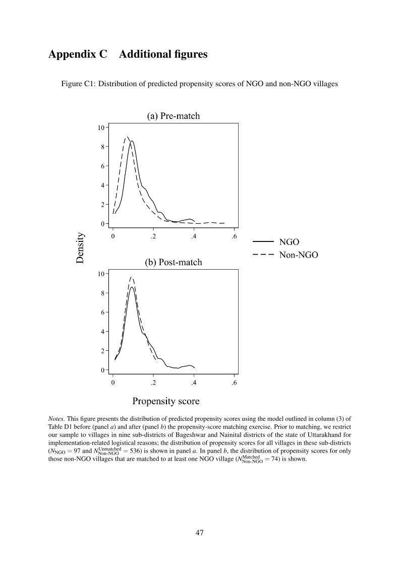
Appendix C Additional figures

Figure C1: Distribution of predicted propensity scores of NGO and non-NGO villages

Notes. This figure presents the distribution of predicted propensity scores using the model outlined in column (3) ofTable D1 before (panel a) and after (panel b) the propensity-score matching exercise. Prior to matching, we restrictour sample to villages in nine sub-districts of Bageshwar and Nainital districts of the state of Uttarakhand forimplementation-related logistical reasons; the distribution of propensity scores for all villages in these sub-districts(NNGO = 97 and NUnmatched

Non-NGO = 536) is shown in panel a. In panel b, the distribution of propensity scores for onlythose non-NGO villages that are matched to at least one NGO village (NMatched

Non-NGO = 74) is shown.

47

Figure C2: Randomization-based inferential procedure applied to village-level stratum allocation

Notes. This figure plots the distribution of 1,000 estimated β3 coefficients from a randomization inference procedure(Athey and Imbens, 2017) applied to village-level NGO stratum allocation to estimate Equation (11). We randomlyassign each village in the sample to placebo NGO and non-NGO strata, and estimate the specification presented incolumn (3) of Table 3 to obtain a placebo “NGO effect” estimate for heterogeneity in purchase of intervention ICS.This procedure is repeated 1,000 times to obtain a distribution of placebo effects. The dark and light grey shadedregions indicate the 90 and 95 percent confidence intervals, respectively, of the placebo distribution. The verticalline indicates the magnitude of our actual estimated “NGO effect,” reported in Table 3.

48

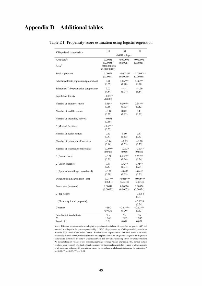
Appendix D Additional tables

Table D1: Propensity-score estimation using logistic regression

Village-level characteristic(1) (2) (3)

✶(NGO village)

Area (km2) 0.00055 0.000096 0.000096(0.00058) (0.00011) (0.00011)

Area2 −0.000000025(0.00000010)

Total population 0.00078 −0.00058* −0.00060**(0.00047) (0.00030) (0.00030)

Scheduled Caste population (proportion) 0.26 1.06*** 1.06***(0.37) (0.28) (0.28)

Scheduled Tribe population (proportion) 7.02 −4.41 −4.59(4.84) (5.07) (5.14)

Population density −0.057*(0.030)

Number of primary schools 0.41** 0.59*** 0.58***(0.18) (0.12) (0.12)

Number of middle schools −0.16 0.080 0.11(0.29) (0.22) (0.22)

Number of secondary schools −0.058(0.60)

✶(Medical facilities) −0.66**(0.33)

Number of health centers 0.63 0.60 0.57(0.87) (0.62) (0.63)

Number of primary health centers −0.44 −0.23 −0.20(0.96) (0.73) (0.73)

Number of telephone connections −0.099** −0.093* −0.094*(0.046) (0.055) (0.056)

✶(Bus services) −0.50 0.65*** 0.62***(0.31) (0.24) (0.24)

✶(Credit societies) 0.31 0.72** 0.71**(0.47) (0.34) (0.34)

✶(Approach to village: paved road) −0.29 −0.43* −0.41*(0.30) (0.23) (0.23)

Distance from nearest town (km) −0.017** −0.016*** −0.015***(0.0081) (0.0045) (0.0045)

Forest area (hectares) 0.00019 0.00026 0.00036(0.00035) (0.00033) (0.00034)

✶(Tap water) −0.0054(0.31)

✶(Electricity for all purposes) −0.0058(0.34)

Constant −19.2 −2.63*** −2.62***(594.4) (0.20) (0.33)

Sub-district fixed effects Yes No NoN 1,960 1,965 1,903Pseudo R2 0.51 0.079 0.077

Notes. This table presents results from logistic regressions of an indicator for whether our partner NGO had

operated in village i in the past—represented by ✶(NGO village)—on a set of village-level characteristics

from the 2001 round of the Indian Census. Standard errors in parentheses. Our final model is shown in

column (3). For this model, we initially restrict our sample to all Census-designated villages in the Bageshwar

and Nainital districts of the state of Uttarakhand with non-zero or non-missing values for total population.

We then exclude six villages where pretesting activities occurred with an alternative NGO partner (details

available upon request). The final estimation sample for the model presented in column (3), thus, consists

of all remaining villages with non-missing values for the village-level characteristics used for estimation. ∗

p < 0.10, ∗∗ p < 0.05, ∗∗∗ p < 0.01.

49

Table D2: Comparison of NGO and non-NGO villages using selected 2011 Census variables

Village-level characteristic(1) (2) (3) (4)

NGO villages Non-NGO villagesMean Normalized

Mean/SD Mean/SD difference difference

Mean household size 4.89 4.49 0.40 0.87[0.45] [0.37]

Number of rooms in mean dwelling 3.14 2.84 0.30 0.38[0.83] [0.74]

Tap water from treated source (%) 48.37 50.36 −1.99 −0.05[40.97] [39.11]

Main lighting source: Electricity (%) 93.42 81.35 12.07 0.91[7.31] [15.16]

Main lighting source: Kerosene (%) 5.38 16.45 −11.07 −0.90[6.81] [14.17]

Fuel used for cooking: Firewood 81.46 81.79 −0.33 −0.02[16.41] [20.98]

Fuel used for cooking: LPG 16.89 16.31 0.58 0.03[16.17] [21.22]

Fuel used for cooking: Electricity 0.00 0.06 −0.06 −0.32[0.00] [0.25]

Number of household availing banking services 86.54 84.50 2.04 0.12[14.37] [19.02]

Asset ownership: Radio (%) 20.85 22.22 −1.37 −0.08[16.34] [17.23]

Asset ownership: Television (%) 50.15 40.43 9.72 0.48[20.05] [20.21]

Asset ownership: Mobile phone (%) 58.65 58.66 −0.01 −0.00[25.27] [20.87]

Asset ownership: Bicycle (%) 1.67 0.97 0.70 0.27[2.83] [2.44]

Asset ownership: Scooter (%) 2.95 2.65 0.30 0.07[4.07] [4.27]

Asset ownership: Car (%) 1.05 1.92 −0.87 −0.48[1.51] [2.03]

N 19 19 38

Notes. Columns (1) and (2) show means and standard deviations (in brackets) for NGO and non-NGO villages, respectively, for selected

village-level variables from the 2011 round of the Indian Census; column (3) shows the difference between the means in columns (1) and

(2); and column (4) shows the normalized difference between the means in columns (1) and (2). “Mean household size” is calculated using

data on the village-level distribution of household sizes, assuming that the category “6–8” contains households with six members and the

category “9+” contains households with nine members. “Number of rooms in mean dwelling” is similarly calculated using data on the

village-level distribution of dwelling size, assuming that the category “six rooms and above” contains dwellings with six rooms. p-values

associated with differences in means are obtained from a regression model of the form: Yid = β1 ·✶(NGO villagei)+ γd + εid , where Yid

represents a village-level characteristic for village i in district d; ✶(NGO villagei) represents an indicator that equals one if our partner NGO

had operated in village i in the past; γd is district fixed-effect; and εid represents a normally distributed error term. Standard errors (not

shown) are robust to heteroskedasticity, and p-values are adjusted using the free step-down resampling methodology of Westfall and Young

(1993), as operationalized by Jones et al. (2019). ∗ p < 0.10, ∗∗ p < 0.05, ∗∗∗ p < 0.01.

50

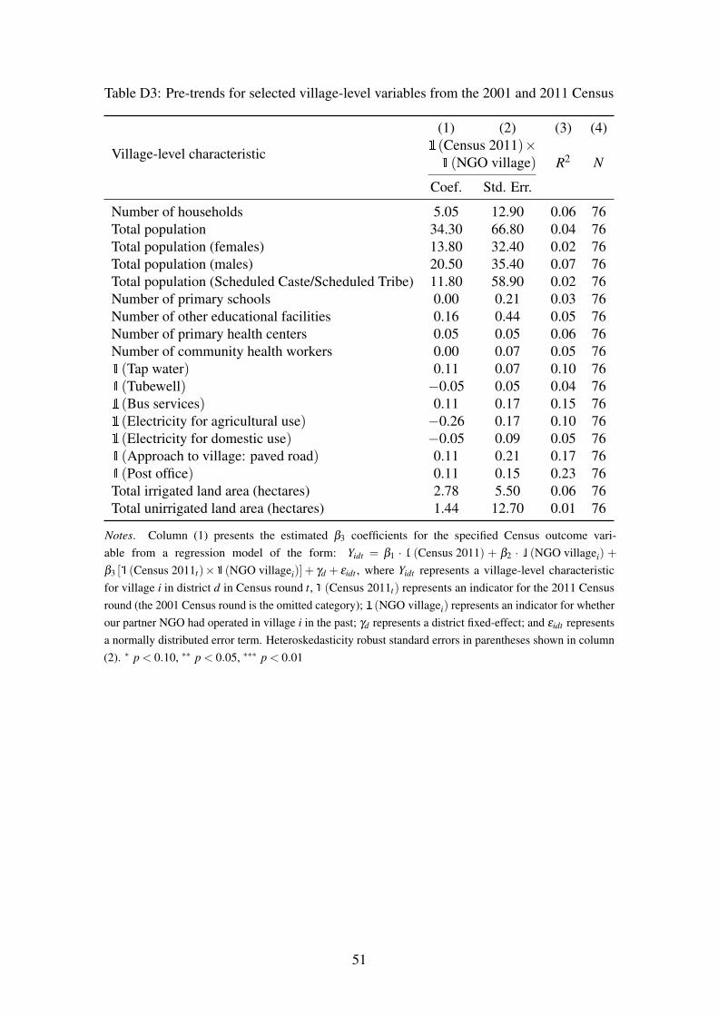
Table D3: Pre-trends for selected village-level variables from the 2001 and 2011 Census

Village-level characteristic

(1) (2) (3) (4)✶(Census 2011)×

R2 N✶(NGO village)

Coef. Std. Err.

Number of households 5.05 12.90 0.06 76Total population 34.30 66.80 0.04 76Total population (females) 13.80 32.40 0.02 76Total population (males) 20.50 35.40 0.07 76Total population (Scheduled Caste/Scheduled Tribe) 11.80 58.90 0.02 76Number of primary schools 0.00 0.21 0.03 76Number of other educational facilities 0.16 0.44 0.05 76Number of primary health centers 0.05 0.05 0.06 76Number of community health workers 0.00 0.07 0.05 76✶(Tap water) 0.11 0.07 0.10 76✶(Tubewell) −0.05 0.05 0.04 76✶(Bus services) 0.11 0.17 0.15 76✶(Electricity for agricultural use) −0.26 0.17 0.10 76✶(Electricity for domestic use) −0.05 0.09 0.05 76✶(Approach to village: paved road) 0.11 0.21 0.17 76✶(Post office) 0.11 0.15 0.23 76Total irrigated land area (hectares) 2.78 5.50 0.06 76Total unirrigated land area (hectares) 1.44 12.70 0.01 76

Notes. Column (1) presents the estimated β3 coefficients for the specified Census outcome vari-

able from a regression model of the form: Yidt = β1 · ✶(Census 2011) + β2 · ✶(NGO villagei) +

β3 [✶(Census 2011t)×✶(NGO villagei)] + γd + εidt , where Yidt represents a village-level characteristic

for village i in district d in Census round t, ✶(Census 2011t) represents an indicator for the 2011 Census

round (the 2001 Census round is the omitted category); ✶(NGO villagei) represents an indicator for whether

our partner NGO had operated in village i in the past; γd represents a district fixed-effect; and εidt represents

a normally distributed error term. Heteroskedasticity robust standard errors in parentheses shown in column

(2). ∗ p < 0.10, ∗∗ p < 0.05, ∗∗∗ p < 0.01

51

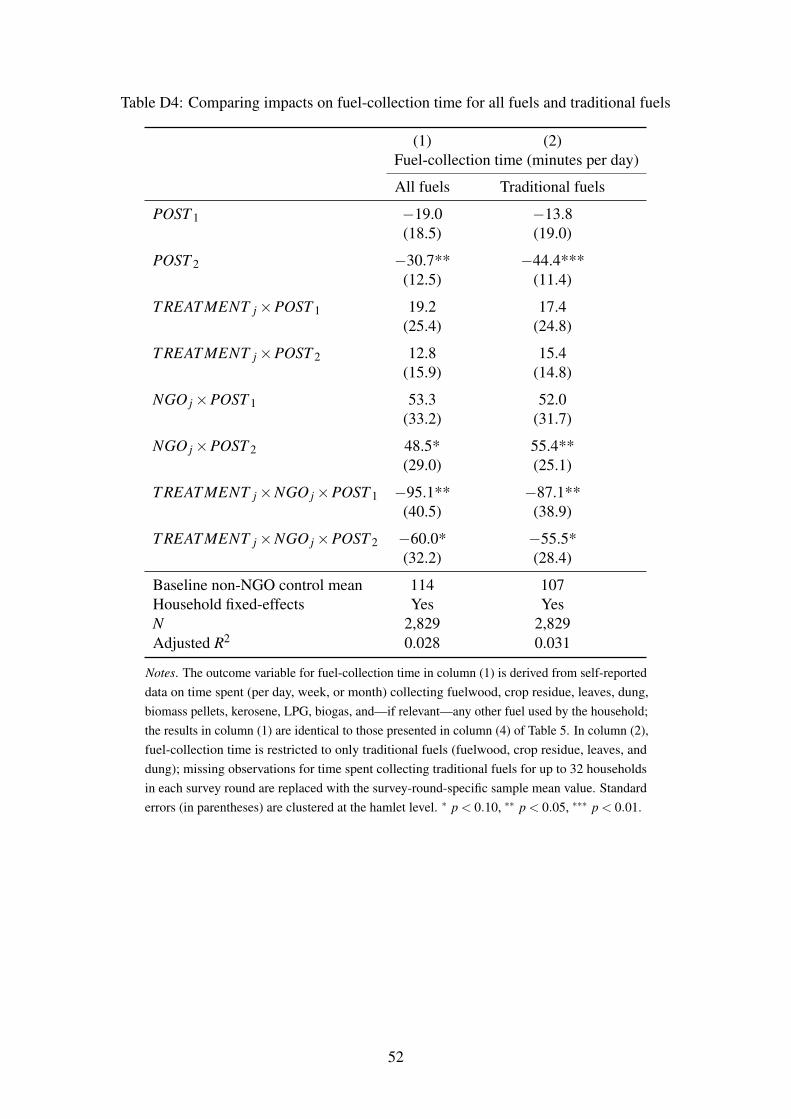
Table D4: Comparing impacts on fuel-collection time for all fuels and traditional fuels

(1) (2)Fuel-collection time (minutes per day)

All fuels Traditional fuels

POST 1 −19.0 −13.8(18.5) (19.0)

POST 2 −30.7** −44.4***(12.5) (11.4)

T REAT MENT j ×POST 1 19.2 17.4(25.4) (24.8)

T REAT MENT j ×POST 2 12.8 15.4(15.9) (14.8)

NGO j ×POST 1 53.3 52.0(33.2) (31.7)

NGO j ×POST 2 48.5* 55.4**(29.0) (25.1)

T REAT MENT j ×NGO j ×POST 1 −95.1** −87.1**(40.5) (38.9)

T REAT MENT j ×NGO j ×POST 2 −60.0* −55.5*(32.2) (28.4)

Baseline non-NGO control mean 114 107Household fixed-effects Yes YesN 2,829 2,829Adjusted R2 0.028 0.031

Notes. The outcome variable for fuel-collection time in column (1) is derived from self-reported

data on time spent (per day, week, or month) collecting fuelwood, crop residue, leaves, dung,

biomass pellets, kerosene, LPG, biogas, and—if relevant—any other fuel used by the household;

the results in column (1) are identical to those presented in column (4) of Table 5. In column (2),

fuel-collection time is restricted to only traditional fuels (fuelwood, crop residue, leaves, and

dung); missing observations for time spent collecting traditional fuels for up to 32 households

in each survey round are replaced with the survey-round-specific sample mean value. Standard

errors (in parentheses) are clustered at the hamlet level. ∗ p < 0.10, ∗∗ p < 0.05, ∗∗∗ p < 0.01.

52

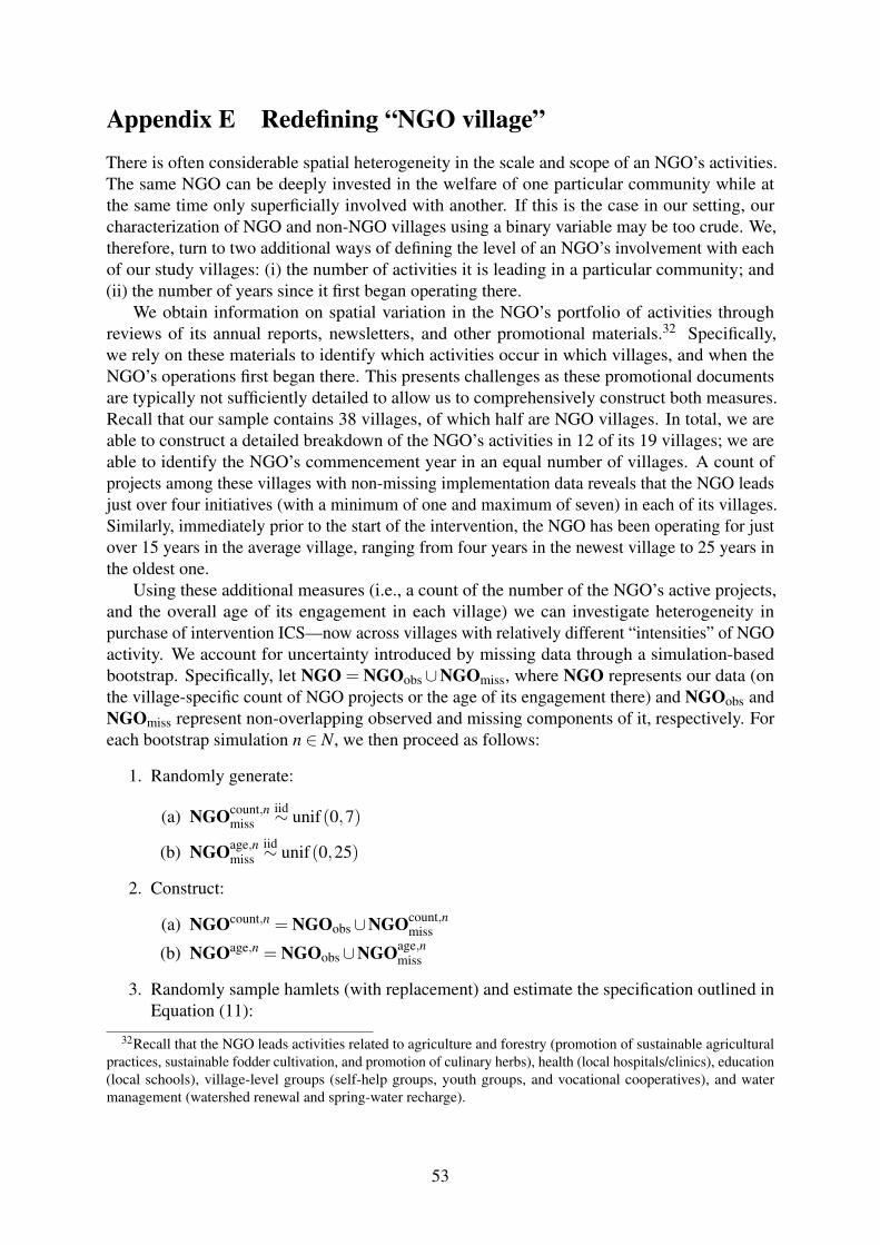
Appendix E Redefining “NGO village”

There is often considerable spatial heterogeneity in the scale and scope of an NGO’s activities.The same NGO can be deeply invested in the welfare of one particular community while atthe same time only superficially involved with another. If this is the case in our setting, ourcharacterization of NGO and non-NGO villages using a binary variable may be too crude. We,therefore, turn to two additional ways of defining the level of an NGO’s involvement with eachof our study villages: (i) the number of activities it is leading in a particular community; and(ii) the number of years since it first began operating there.

We obtain information on spatial variation in the NGO’s portfolio of activities throughreviews of its annual reports, newsletters, and other promotional materials.32 Specifically,we rely on these materials to identify which activities occur in which villages, and when theNGO’s operations first began there. This presents challenges as these promotional documentsare typically not sufficiently detailed to allow us to comprehensively construct both measures.Recall that our sample contains 38 villages, of which half are NGO villages. In total, we areable to construct a detailed breakdown of the NGO’s activities in 12 of its 19 villages; we areable to identify the NGO’s commencement year in an equal number of villages. A count ofprojects among these villages with non-missing implementation data reveals that the NGO leadsjust over four initiatives (with a minimum of one and maximum of seven) in each of its villages.Similarly, immediately prior to the start of the intervention, the NGO has been operating for justover 15 years in the average village, ranging from four years in the newest village to 25 years inthe oldest one.

Using these additional measures (i.e., a count of the number of the NGO’s active projects,and the overall age of its engagement in each village) we can investigate heterogeneity inpurchase of intervention ICS—now across villages with relatively different “intensities” of NGOactivity. We account for uncertainty introduced by missing data through a simulation-basedbootstrap. Specifically, let NGO = NGOobs ∪NGOmiss, where NGO represents our data (onthe village-specific count of NGO projects or the age of its engagement there) and NGOobs andNGOmiss represent non-overlapping observed and missing components of it, respectively. Foreach bootstrap simulation n ∈ N, we then proceed as follows:

1. Randomly generate:

(a) NGOcount,nmiss

iid∼ unif(0,7)

(b) NGOage,nmiss

iid∼ unif(0,25)

2. Construct:

(a) NGOcount,n = NGOobs ∪NGOcount,nmiss

(b) NGOage,n = NGOobs ∪NGOage,nmiss

3. Randomly sample hamlets (with replacement) and estimate the specification outlined inEquation (11):

32Recall that the NGO leads activities related to agriculture and forestry (promotion of sustainable agriculturalpractices, sustainable fodder cultivation, and promotion of culinary herbs), health (local hospitals/clinics), education(local schools), village-level groups (self-help groups, youth groups, and vocational cooperatives), and watermanagement (watershed renewal and spring-water recharge).

53

(a)

Ycount,ni jd = β count,n

1

(T REAT MENT j

)+β count,n

2

(

NGOcount,nj

)

+

+β count,n3

(

T REAT MENT j ×NGOcount,nj

)

+Xiδ+ γd +νi j

(b)

Yage,ni jd = β

age,n1

(T REAT MENT j

)+β

age,n2

(

NGOage,nj

)

+

+βage,n3

(

T REAT MENT j ×NGOage,nj

)

+Xiδ+ γd +νi j

4. Save the estimated regression coefficients:

(a) β̂ count,n3

(b) β̂age,n3

In other words, for villages lacking data on the count of projects, we replace missing countobservations with random draws from a uniform distribution over the interval lying between theminimum (i.e., zero in non-NGO villages) and maximum (seven) number of projects observedin each village in our data. For villages lacking data on the age of NGO engagement, wesimilarly replace missing observations with random draws from a uniform distribution over theinterval lying between the minimum (zero in non-NGO villages) and maximum (25) ages in ourdata. Having replaced these missing observations, we sample hamlets (with replacement) fromour study sample to generate a bootstrapped sample, and separately estimate the specificationoutlined in Equation (11) by replacing our NGO binary variable with the count of NGO activitiesor the age of NGO engagement. For each specification, we repeat this process 10,000 times toobtain a distribution of the estimated coefficient for the T REAT MENT j ×NGO j interactionterm. We note that this is a relatively conservative approach to dealing with the uncertaintysurrounding missing observations. It is almost certainly the case that the NGO has activeprojects in each of its villages, and has operated in them for at least a few years. Nevertheless,the uniform distributions we use to replace missing observations have positive support overzero (the value these variables are assigned for non-NGO villages). In addition, our randomlygenerated replacements never exceed the maximum value observed in the (non-missing) data.

Figure E1 presents our results. As shown in panel a, we find that purchase rates by house-holds in treated NGO hamlets are, on average, approximately two percentage points higher forevery additional project that the NGO leads in that particular village. This result is statisticallysignificant at the 10 percent level, as measured by the 90 percent confidence interval of thedistribution of our simulated regression coefficients. Similarly, panel b shows that every addi-tional year of the NGO’s presence in a village resulted in an increase in rates of ICS purchase byhouseholds in treated NGO hamlets by just under one percentage point. Broadly, these resultsserve as a robustness check for our main result (Table 3). They are also consistent with ourmodel and show that NGO activity—defined in a variety of ways—influences the effectivenessof interventions.

54

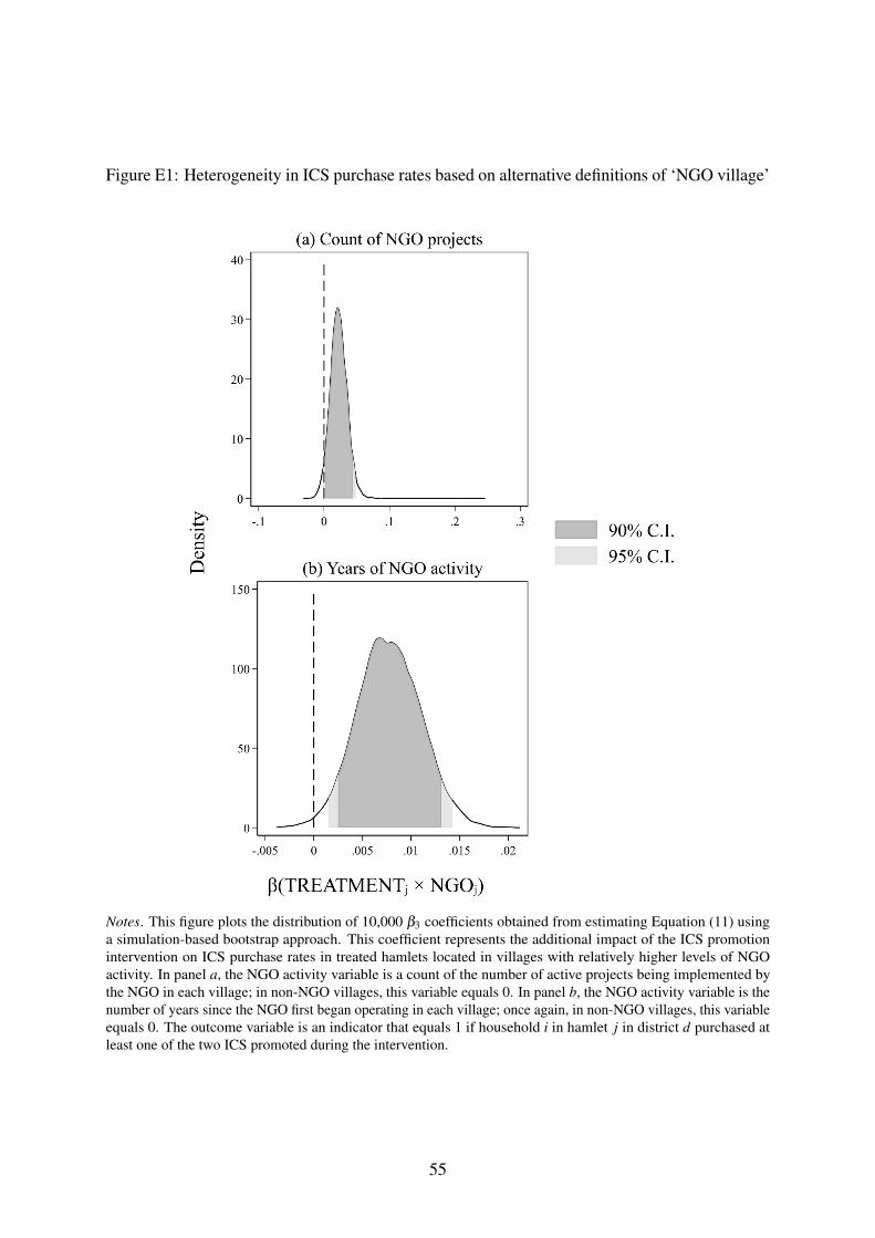
Figure E1: Heterogeneity in ICS purchase rates based on alternative definitions of ‘NGO village’

Notes. This figure plots the distribution of 10,000 β3 coefficients obtained from estimating Equation (11) usinga simulation-based bootstrap approach. This coefficient represents the additional impact of the ICS promotionintervention on ICS purchase rates in treated hamlets located in villages with relatively higher levels of NGOactivity. In panel a, the NGO activity variable is a count of the number of active projects being implemented bythe NGO in each village; in non-NGO villages, this variable equals 0. In panel b, the NGO activity variable is thenumber of years since the NGO first began operating in each village; once again, in non-NGO villages, this variableequals 0. The outcome variable is an indicator that equals 1 if household i in hamlet j in district d purchased atleast one of the two ICS promoted during the intervention.

55

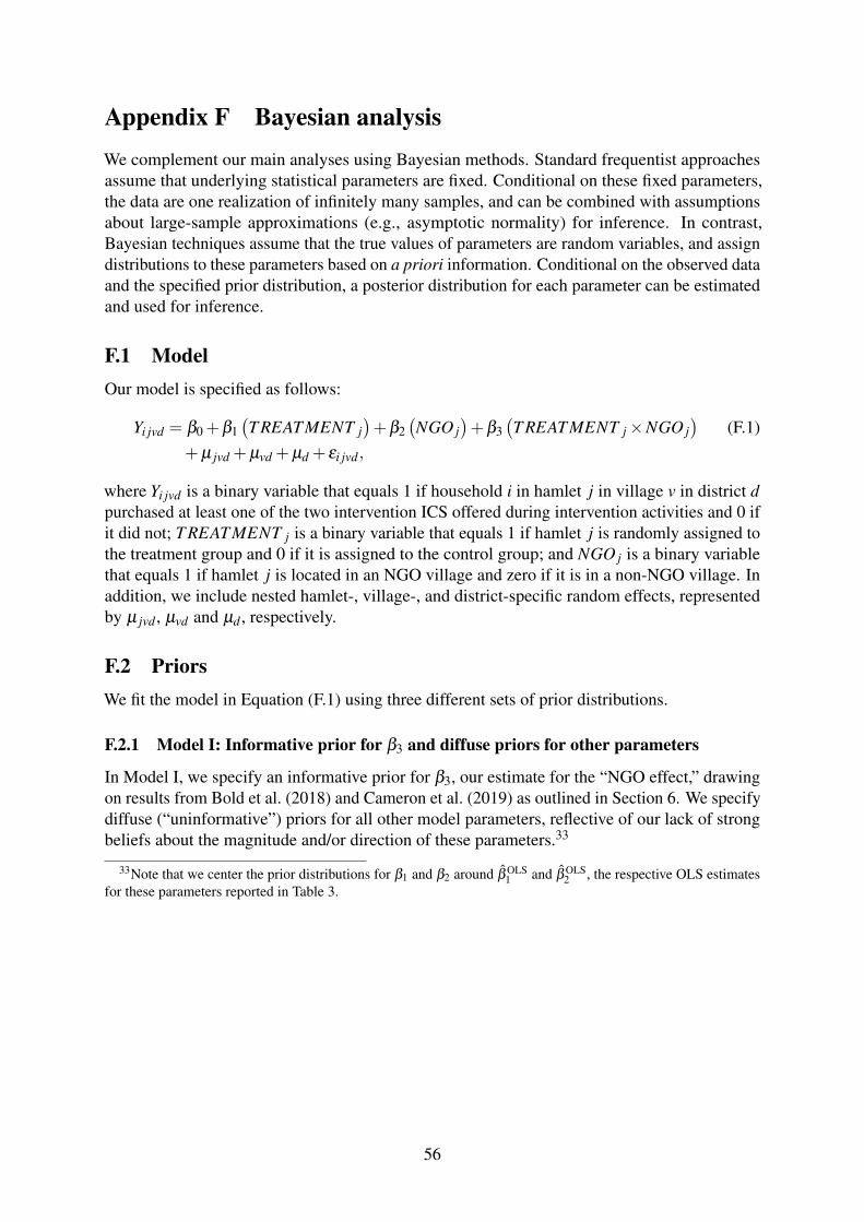
Appendix F Bayesian analysis

We complement our main analyses using Bayesian methods. Standard frequentist approachesassume that underlying statistical parameters are fixed. Conditional on these fixed parameters,the data are one realization of infinitely many samples, and can be combined with assumptionsabout large-sample approximations (e.g., asymptotic normality) for inference. In contrast,Bayesian techniques assume that the true values of parameters are random variables, and assigndistributions to these parameters based on a priori information. Conditional on the observed dataand the specified prior distribution, a posterior distribution for each parameter can be estimatedand used for inference.

F.1 Model

Our model is specified as follows:

Yi jvd = β0 +β1(T REAT MENT j

)+β2

(NGO j

)+β3

(T REAT MENT j ×NGO j

)(F.1)

+µ jvd +µvd +µd + εi jvd,

where Yi jvd is a binary variable that equals 1 if household i in hamlet j in village v in district d

purchased at least one of the two intervention ICS offered during intervention activities and 0 ifit did not; T REAT MENT j is a binary variable that equals 1 if hamlet j is randomly assigned tothe treatment group and 0 if it is assigned to the control group; and NGO j is a binary variablethat equals 1 if hamlet j is located in an NGO village and zero if it is in a non-NGO village. Inaddition, we include nested hamlet-, village-, and district-specific random effects, representedby µ jvd , µvd and µd , respectively.

F.2 Priors

We fit the model in Equation (F.1) using three different sets of prior distributions.

F.2.1 Model I: Informative prior for β3 and diffuse priors for other parameters

In Model I, we specify an informative prior for β3, our estimate for the “NGO effect,” drawingon results from Bold et al. (2018) and Cameron et al. (2019) as outlined in Section 6. We specifydiffuse (“uninformative”) priors for all other model parameters, reflective of our lack of strongbeliefs about the magnitude and/or direction of these parameters.33

33Note that we center the prior distributions for β1 and β2 around β̂ OLS1 and β̂ OLS

2 , the respective OLS estimatesfor these parameters reported in Table 3.

56

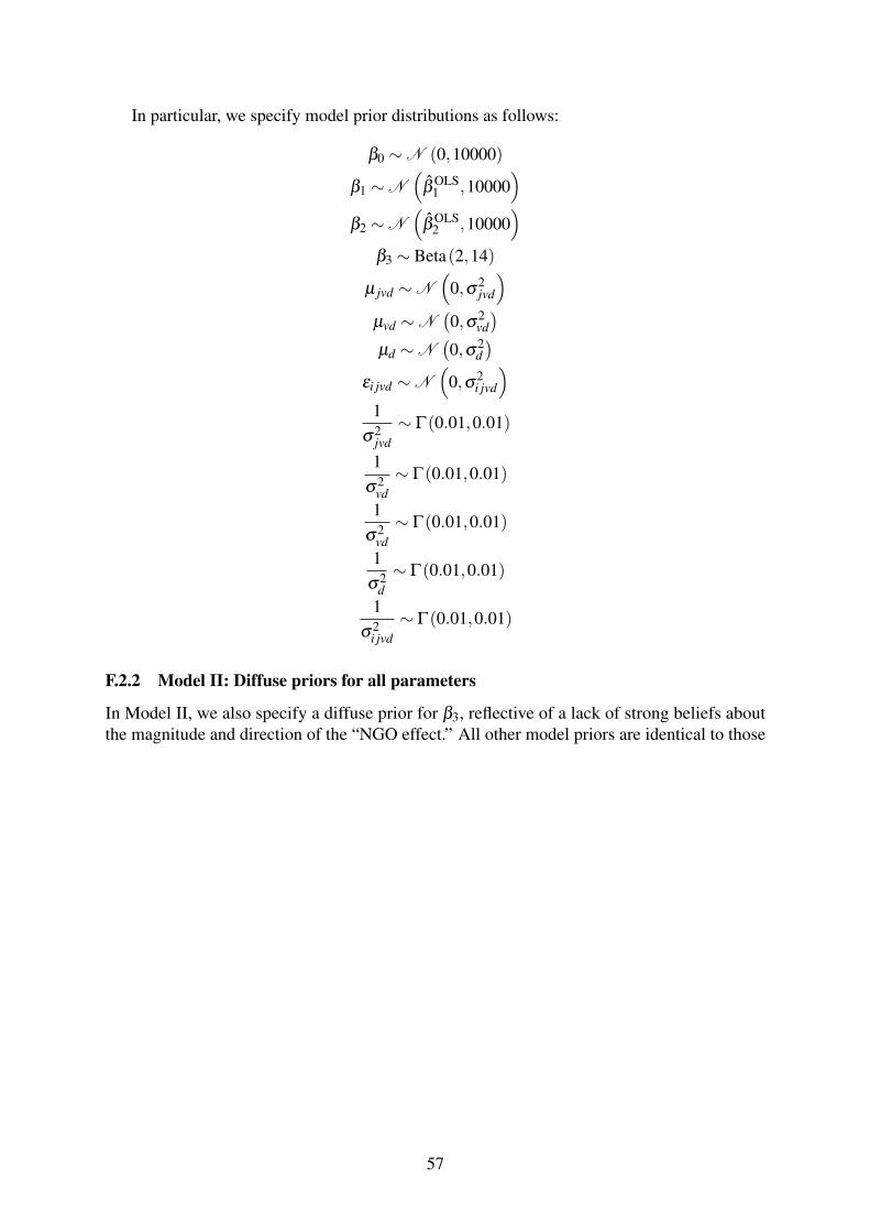
In particular, we specify model prior distributions as follows:

β0 ∼ N (0,10000)

β1 ∼ N

(

β̂ OLS1 ,10000

)

β2 ∼ N

(

β̂ OLS2 ,10000

)

β3 ∼ Beta(2,14)

µ jvd ∼ N

(

0,σ2jvd

)

µvd ∼ N(0,σ2

vd

)

µd ∼ N(0,σ2

d

)

εi jvd ∼ N

(

0,σ2i jvd

)

1

σ2jvd

∼ Γ(0.01,0.01)

1

σ2vd

∼ Γ(0.01,0.01)

1

σ2vd

∼ Γ(0.01,0.01)

1

σ2d

∼ Γ(0.01,0.01)

1

σ2i jvd

∼ Γ(0.01,0.01)

F.2.2 Model II: Diffuse priors for all parameters

In Model II, we also specify a diffuse prior for β3, reflective of a lack of strong beliefs aboutthe magnitude and direction of the “NGO effect.” All other model priors are identical to those

57

specified in Model I, as follows:

β0 ∼ N (0,10000)

β1 ∼ N

(

β̂ OLS1 ,10000

)

β2 ∼ N

(

β̂ OLS2 ,10000

)

β3 ∼ N

(

β̂ OLS3 ,10000

)

µ jvd ∼ N

(

0,σ2jvd

)

µvd ∼ N(0,σ2

vd

)

µd ∼ N(0,σ2

d

)

εi jvd ∼ N

(

0,σ2i jvd

)

1

σ2jvd

∼ Γ(0.01,0.01)

1

σ2vd

∼ Γ(0.01,0.01)

1

σ2vd

∼ Γ(0.01,0.01)

1

σ2d

∼ Γ(0.01,0.01)

1

σ2i jvd

∼ Γ(0.01,0.01)

F.2.3 Model III: Strong no-NGO-effect prior for β3 and diffuse priors for other param-

eters

Finally, in Model III, we specify a “strong” prior for β3 that is centered around zero, reflectiveof the prior beliefs that the magnitude of the “NGO effect” is negligible. Once again, all other

58

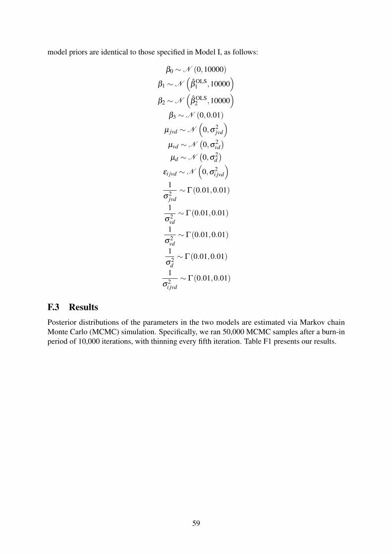
model priors are identical to those specified in Model I, as follows:

β0 ∼ N (0,10000)

β1 ∼ N

(

β̂ OLS1 ,10000

)

β2 ∼ N

(

β̂ OLS2 ,10000

)

β3 ∼ N (0,0.01)

µ jvd ∼ N

(

0,σ2jvd

)

µvd ∼ N(0,σ2

vd

)

µd ∼ N(0,σ2

d

)

εi jvd ∼ N

(

0,σ2i jvd

)

1

σ2jvd

∼ Γ(0.01,0.01)

1

σ2vd

∼ Γ(0.01,0.01)

1

σ2vd

∼ Γ(0.01,0.01)

1

σ2d

∼ Γ(0.01,0.01)

1

σ2i jvd

∼ Γ(0.01,0.01)

F.3 Results

Posterior distributions of the parameters in the two models are estimated via Markov chainMonte Carlo (MCMC) simulation. Specifically, we ran 50,000 MCMC samples after a burn-inperiod of 10,000 iterations, with thinning every fifth iteration. Table F1 presents our results.

59

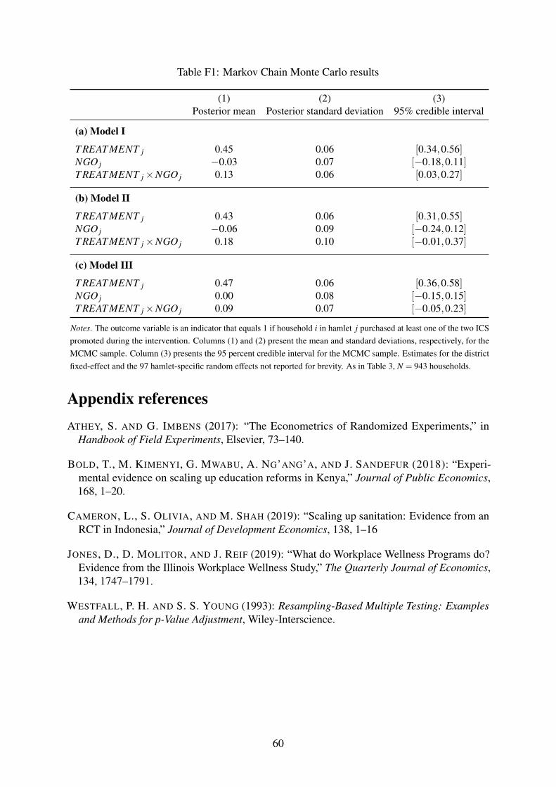
Table F1: Markov Chain Monte Carlo results

(1) (2) (3)Posterior mean Posterior standard deviation 95% credible interval

(a) Model I

T REAT MENT j 0.45 0.06 [0.34,0.56]NGO j −0.03 0.07 [−0.18,0.11]T REAT MENT j ×NGO j 0.13 0.06 [0.03,0.27]

(b) Model II

T REAT MENT j 0.43 0.06 [0.31,0.55]NGO j −0.06 0.09 [−0.24,0.12]T REAT MENT j ×NGO j 0.18 0.10 [−0.01,0.37]

(c) Model III

T REAT MENT j 0.47 0.06 [0.36,0.58]NGO j 0.00 0.08 [−0.15,0.15]T REAT MENT j ×NGO j 0.09 0.07 [−0.05,0.23]

Notes. The outcome variable is an indicator that equals 1 if household i in hamlet j purchased at least one of the two ICS

promoted during the intervention. Columns (1) and (2) present the mean and standard deviations, respectively, for the

MCMC sample. Column (3) presents the 95 percent credible interval for the MCMC sample. Estimates for the district

fixed-effect and the 97 hamlet-specific random effects not reported for brevity. As in Table 3, N = 943 households.

Appendix references

ATHEY, S. AND G. IMBENS (2017): “The Econometrics of Randomized Experiments,” inHandbook of Field Experiments, Elsevier, 73–140.

BOLD, T., M. KIMENYI, G. MWABU, A. NG’ANG’A, AND J. SANDEFUR (2018): “Experi-mental evidence on scaling up education reforms in Kenya,” Journal of Public Economics,168, 1–20.

CAMERON, L., S. OLIVIA, AND M. SHAH (2019): “Scaling up sanitation: Evidence from anRCT in Indonesia,” Journal of Development Economics, 138, 1–16

JONES, D., D. MOLITOR, AND J. REIF (2019): “What do Workplace Wellness Programs do?Evidence from the Illinois Workplace Wellness Study,” The Quarterly Journal of Economics,134, 1747–1791.

WESTFALL, P. H. AND S. S. YOUNG (1993): Resampling-Based Multiple Testing: Examples

and Methods for p-Value Adjustment, Wiley-Interscience.

60