1

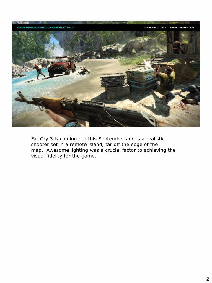
Far Cry 3 is coming out this September and is a realistic shooter set in a remote island, far off the edge of the map. Awesome lighting was a crucial factor to achieving the visual fidelity for the game.

2

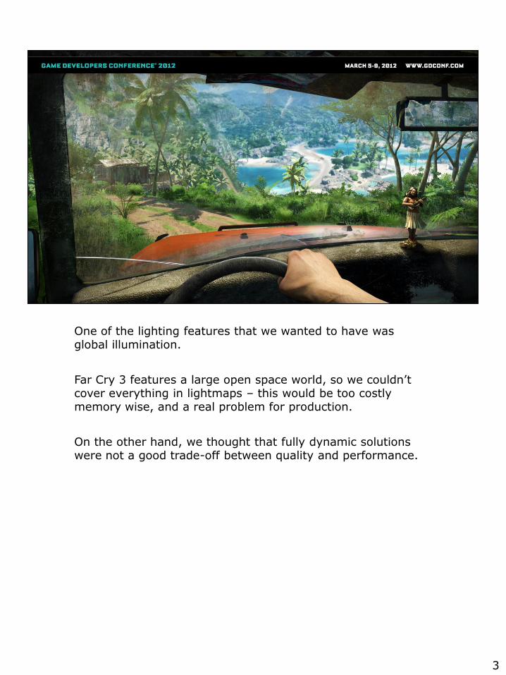
One of the lighting features that we wanted to have was global illumination.

Far Cry 3 features a large open space world, so we couldn’t cover everything in lightmaps – this would be too costly memory wise, and a real problem for production.

On the other hand, we thought that fully dynamic solutions were not a good trade-off between quality and performance.

3

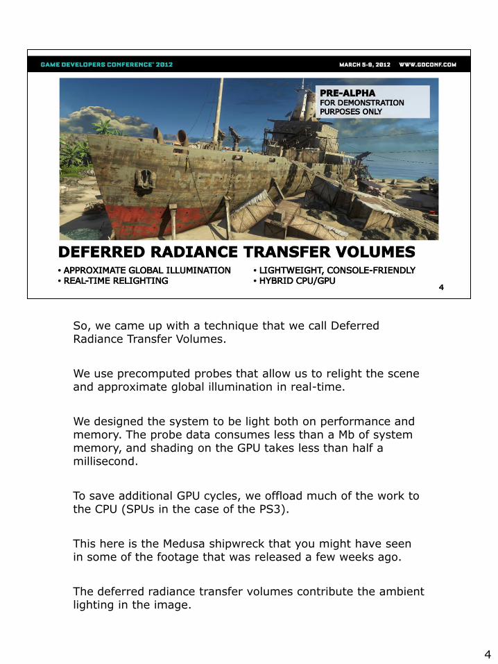
So, we came up with a technique that we call Deferred Radiance Transfer Volumes.

We use precomputed probes that allow us to relight the scene and approximate global illumination in real-time.

We designed the system to be light both on performance and memory. The probe data consumes less than a Mb of system memory, and shading on the GPU takes less than half a millisecond.

To save additional GPU cycles, we offload much of the work to the CPU (SPUs in the case of the PS3).

This here is the Medusa shipwreck that you might have seen in some of the footage that was released a few weeks ago.

The deferred radiance transfer volumes contribute the ambient lighting in the image.

4

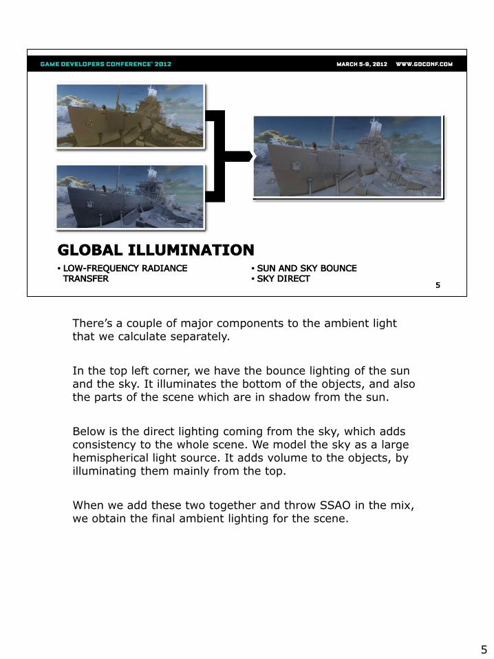
There’s a couple of major components to the ambient light that we calculate separately.

In the top left corner, we have the bounce lighting of the sun and the sky. It illuminates the bottom of the objects, and also the parts of the scene which are in shadow from the sun.

Below is the direct lighting coming from the sky, which adds consistency to the whole scene. We model the sky as a large hemispherical light source. It adds volume to the objects, by illuminating them mainly from the top.

When we add these two together and throw SSAO in the mix, we obtain the final ambient lighting for the scene.

5

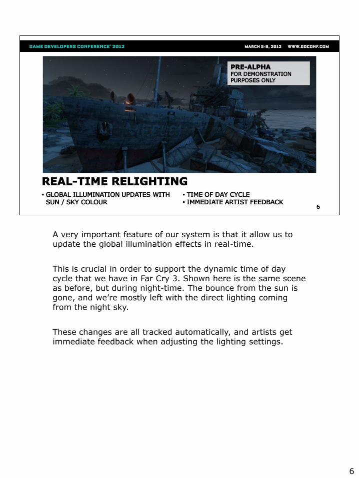
A very important feature of our system is that it allow us to update the global illumination effects in real-time.

This is crucial in order to support the dynamic time of day cycle that we have in Far Cry 3. Shown here is the same scene as before, but during night-time. The bounce from the sun is gone, and we’re mostly left with the direct lighting coming from the night sky.

These changes are all tracked automatically, and artists get immediate feedback when adjusting the lighting settings.

6

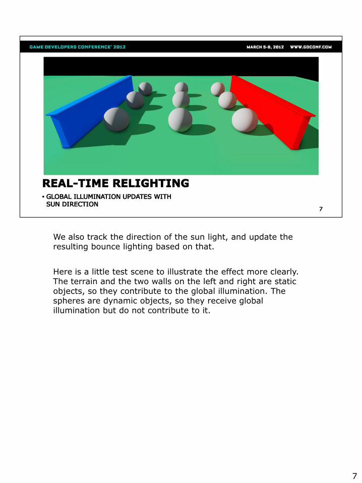
We also track the direction of the sun light, and update the resulting bounce lighting based on that.

Here is a little test scene to illustrate the effect more clearly. The terrain and the two walls on the left and right are static objects, so they contribute to the global illumination. The spheres are dynamic objects, so they receive global illumination but do not contribute to it.

7

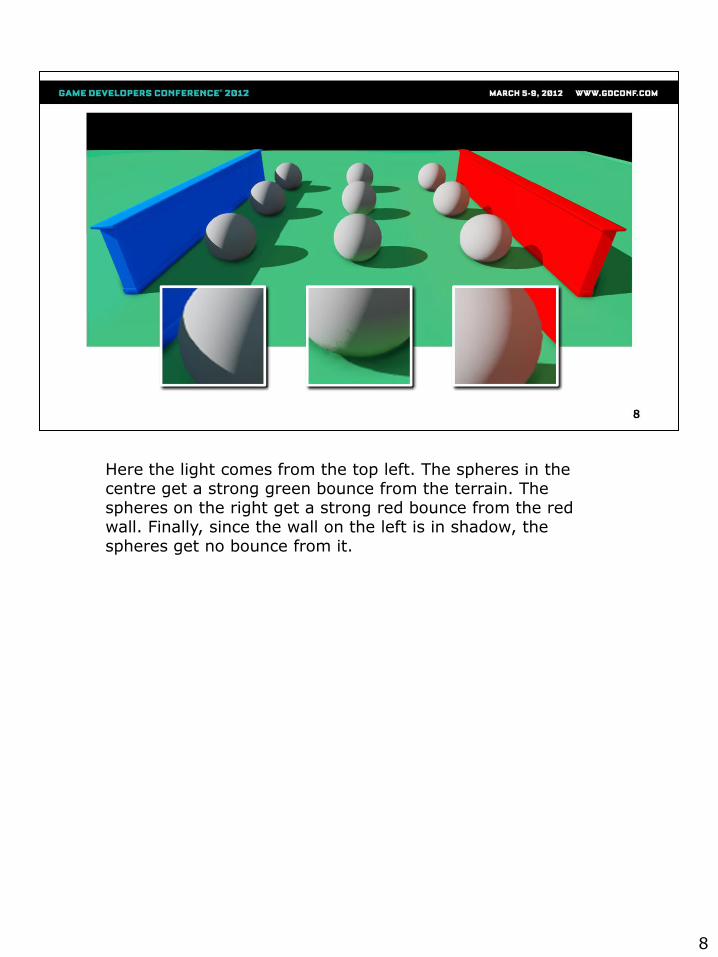
Here the light comes from the top left. The spheres in the centre get a strong green bounce from the terrain. The spheres on the right get a strong red bounce from the red wall. Finally, since the wall on the left is in shadow, the spheres get no bounce from it.

8

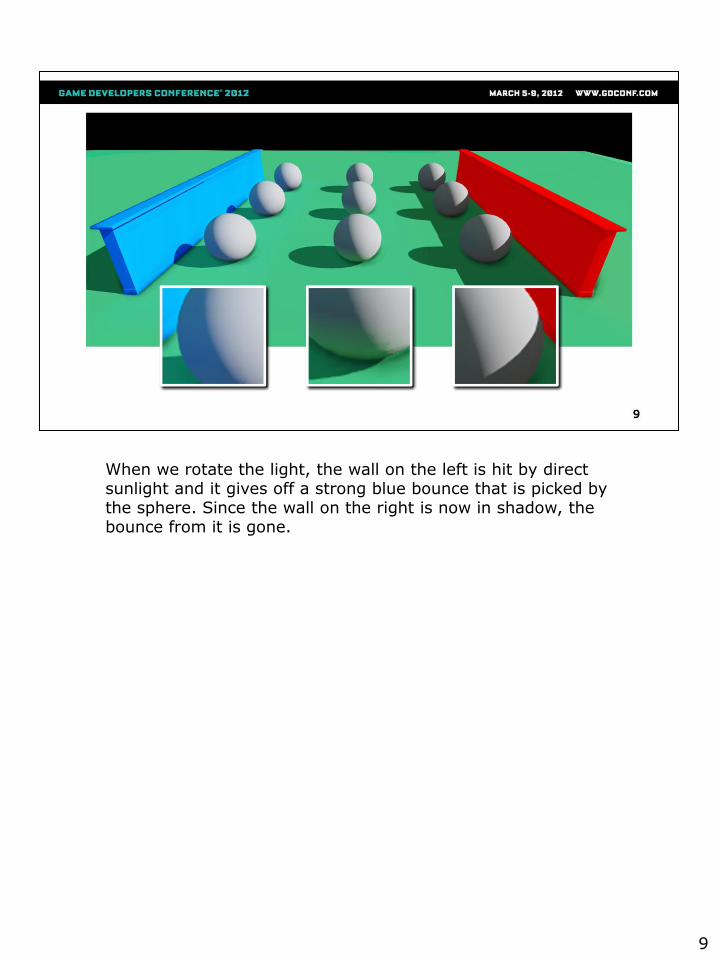
When we rotate the light, the wall on the left is hit by direct sunlight and it gives off a strong blue bounce that is picked by the sphere. Since the wall on the right is now in shadow, the bounce from it is gone.

9

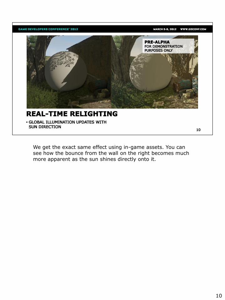
We get the exact same effect using in-game assets. You can see how the bounce from the wall on the right becomes much more apparent as the sun shines directly onto it.

10

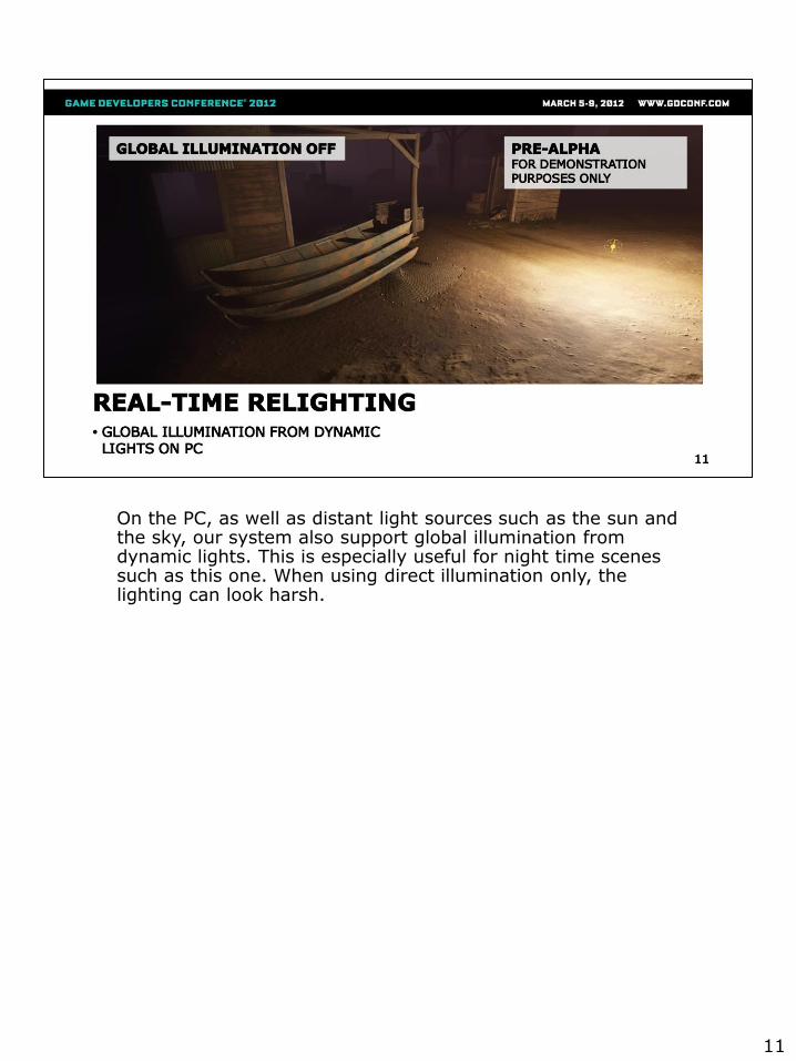
On the PC, as well as distant light sources such as the sun and the sky, our system also support global illumination from dynamic lights. This is especially useful for night time scenes such as this one. When using direct illumination only, the lighting can look harsh.

11

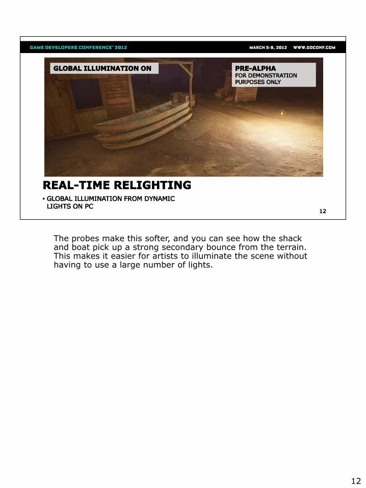
The probes make this softer, and you can see how the shack and boat pick up a strong secondary bounce from the terrain. This makes it easier for artists to illuminate the scene without having to use a large number of lights.

12

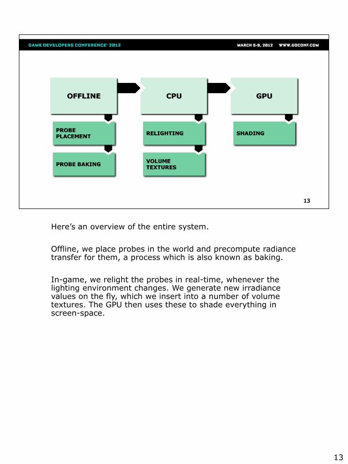
Here’s an overview of the entire system.

Offline, we place probes in the world and precompute radiance transfer for them, a process which is also known as baking.

In-game, we relight the probes in real-time, whenever the lighting environment changes. We generate new irradiance values on the fly, which we insert into a number of volume textures. The GPU then uses these to shade everything in screen-space.

13

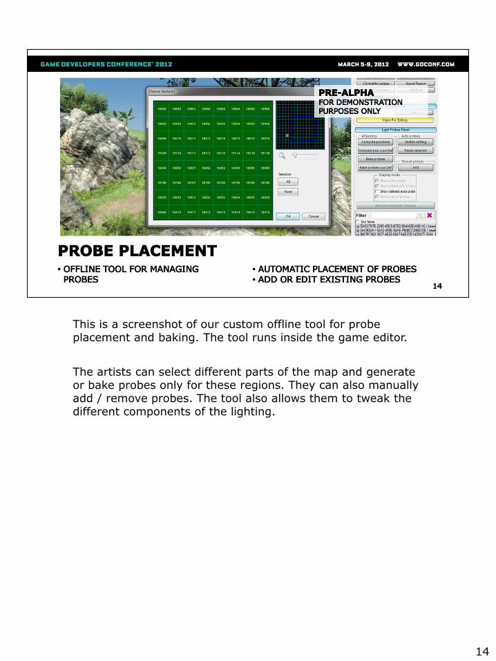
This is a screenshot of our custom offline tool for probe placement and baking. The tool runs inside the game editor.

The artists can select different parts of the map and generate or bake probes only for these regions. They can also manually add / remove probes. The tool also allows them to tweak the different components of the lighting.

14

Because FC3 is a large open world game, it’s inconvenient for artists to place all probes manually. Instead, we automatically spawn new probes at good locations.

To do so, we cast vertical rays every 4 meters along the ground plane. Every time the ray hits a static object or the terrain, we spawn a new probe. We also make sure to keep a minimal distance between hits.

15

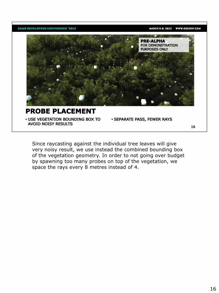
Since raycasting against the individual tree leaves will give very noisy result, we use instead the combined bounding box of the vegetation geometry. In order to not going over budget by spawning too many probes on top of the vegetation, we space the rays every 8 metres instead of 4.

16

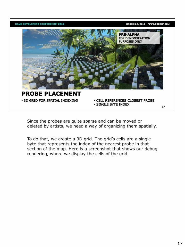
Since the probes are quite sparse and can be moved or deleted by artists, we need a way of organizing them spatially.

To do that, we create a 3D grid. The grid’s cells are a single byte that represents the index of the nearest probe in that section of the map. Here is a screenshot that shows our debug rendering, where we display the cells of the grid.

17

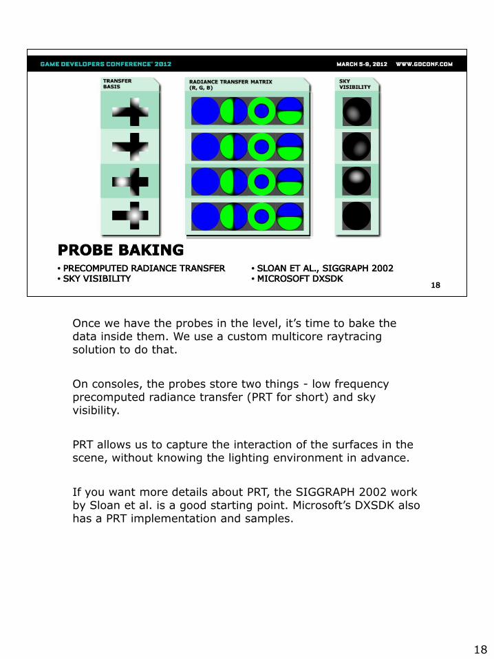
Once we have the probes in the level, it’s time to bake the data inside them. We use a custom multicore raytracingsolution to do that.

On consoles, the probes store two things - low frequency precomputed radiance transfer (PRT for short) and sky visibility.

PRT allows us to capture the interaction of the surfaces in the scene, without knowing the lighting environment in advance.

If you want more details about PRT, the SIGGRAPH 2002 work by Sloan et al. is a good starting point. Microsoft’s DXSDK also has a PRT implementation and samples.

18

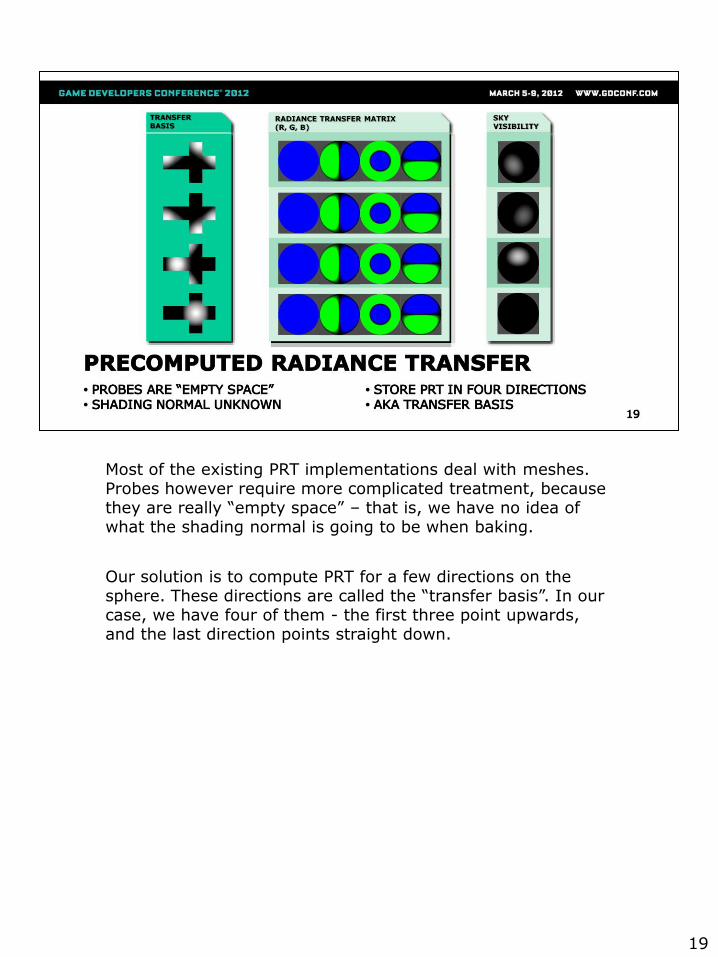
Most of the existing PRT implementations deal with meshes. Probes however require more complicated treatment, because they are really “empty space” – that is, we have no idea of what the shading normal is going to be when baking.

Our solution is to compute PRT for a few directions on the sphere. These directions are called the “transfer basis”. In our case, we have four of them - the first three point upwards, and the last direction points straight down.

19

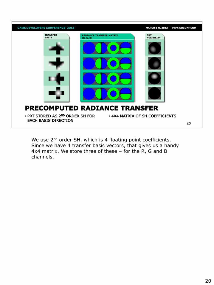
We use 2nd order SH, which is 4 floating point coefficients. Since we have 4 transfer basis vectors, that gives us a handy 4x4 matrix. We store three of these – for the R, G and B channels.

20

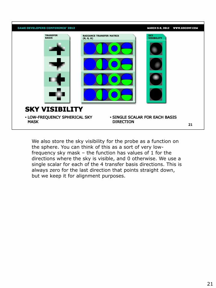
We also store the sky visibility for the probe as a function on the sphere. You can think of this as a sort of very low-frequency sky mask – the function has values of 1 for the directions where the sky is visible, and 0 otherwise. We use a single scalar for each of the 4 transfer basis directions. This is always zero for the last direction that points straight down, but we keep it for alignment purposes.

21

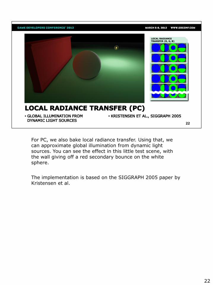
For PC, we also bake local radiance transfer. Using that, we can approximate global illumination from dynamic light sources. You can see the effect in this little test scene, with the wall giving off a red secondary bounce on the white sphere.

The implementation is based on the SIGGRAPH 2005 paper by Kristensen et al.

22

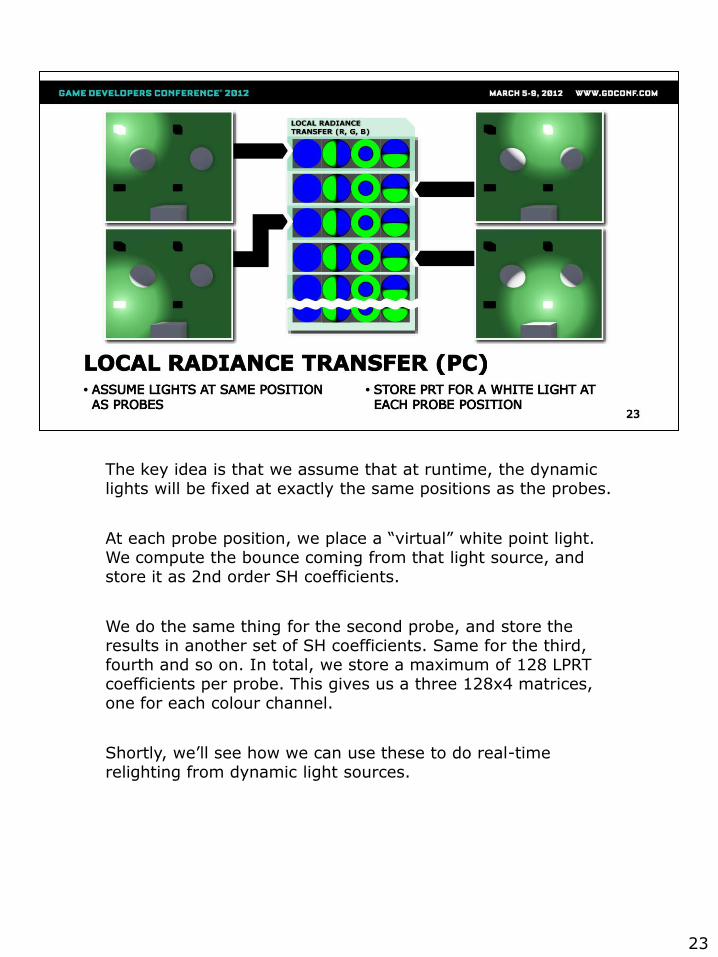
The key idea is that we assume that at runtime, the dynamic lights will be fixed at exactly the same positions as the probes.

At each probe position, we place a “virtual” white point light. We compute the bounce coming from that light source, and store it as 2nd order SH coefficients.

We do the same thing for the second probe, and store the results in another set of SH coefficients. Same for the third, fourth and so on. In total, we store a maximum of 128 LPRT coefficients per probe. This gives us a three 128x4 matrices, one for each colour channel.

Shortly, we’ll see how we can use these to do real-time relighting from dynamic light sources.

23

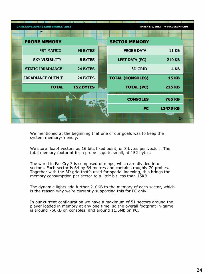
We mentioned at the beginning that one of our goals was to keep the system memory-friendly.

We store float4 vectors as 16 bits fixed point, or 8 bytes per vector. The total memory footprint for a probe is quite small, at 152 bytes.

The world in Far Cry 3 is composed of maps, which are divided intosectors. Each sector is 64 by 64 metres and contains roughly 70 probes. Together with the 3D grid that’s used for spatial indexing, this brings the memory consumption per sector to a little bit less than 15KB.

The dynamic lights add further 210KB to the memory of each sector, which is the reason why we’re currently supporting this for PC only.

In our current configuration we have a maximum of 51 sectors around the player loaded in memory at any one time, so the overall footprint in-game is around 760KB on consoles, and around 11.5Mb on PC.

24

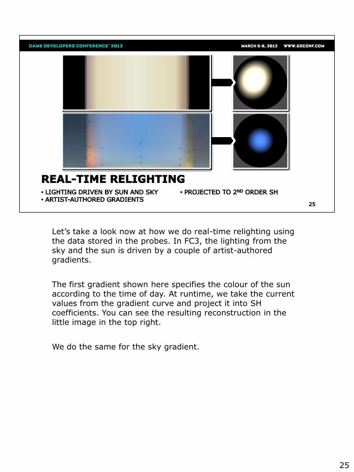
Let’s take a look now at how we do real-time relighting using the data stored in the probes. In FC3, the lighting from the sky and the sun is driven by a couple of artist-authored gradients.

The first gradient shown here specifies the colour of the sun according to the time of day. At runtime, we take the current values from the gradient curve and project it into SH coefficients. You can see the resulting reconstruction in the little image in the top right.

We do the same for the sky gradient.

25

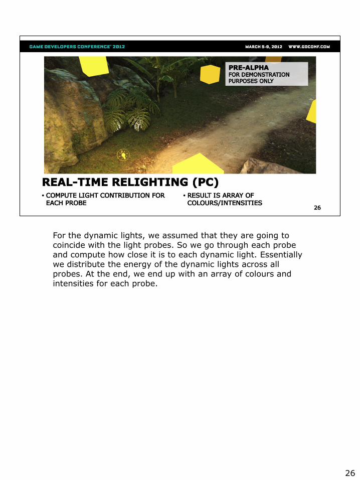
For the dynamic lights, we assumed that they are going to coincide with the light probes. So we go through each probe and compute how close it is to each dynamic light. Essentially we distribute the energy of the dynamic lights across all probes. At the end, we end up with an array of colours and intensities for each probe.

26

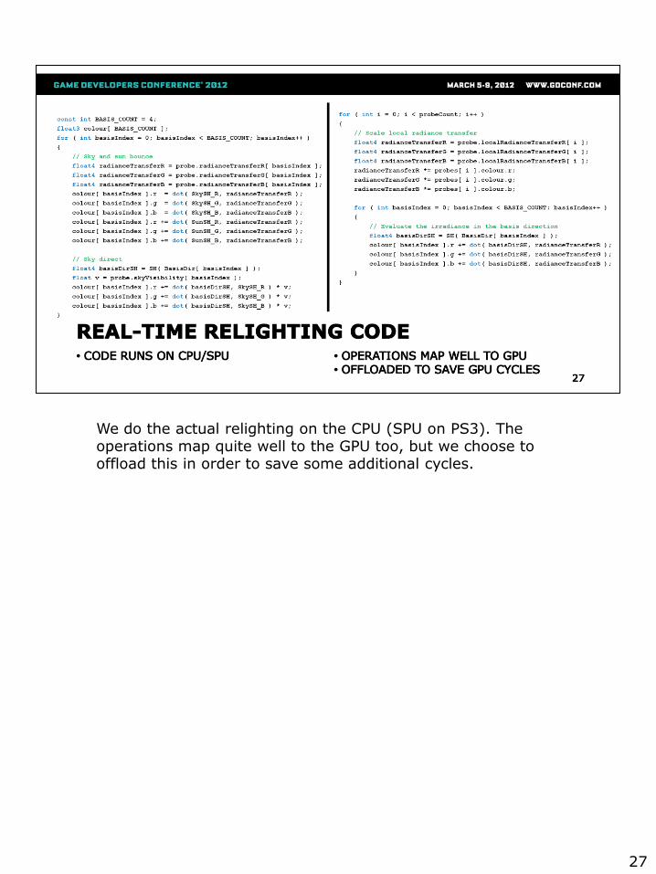
We do the actual relighting on the CPU (SPU on PS3). The operations map quite well to the GPU too, but we choose to offload this in order to save some additional cycles.

27

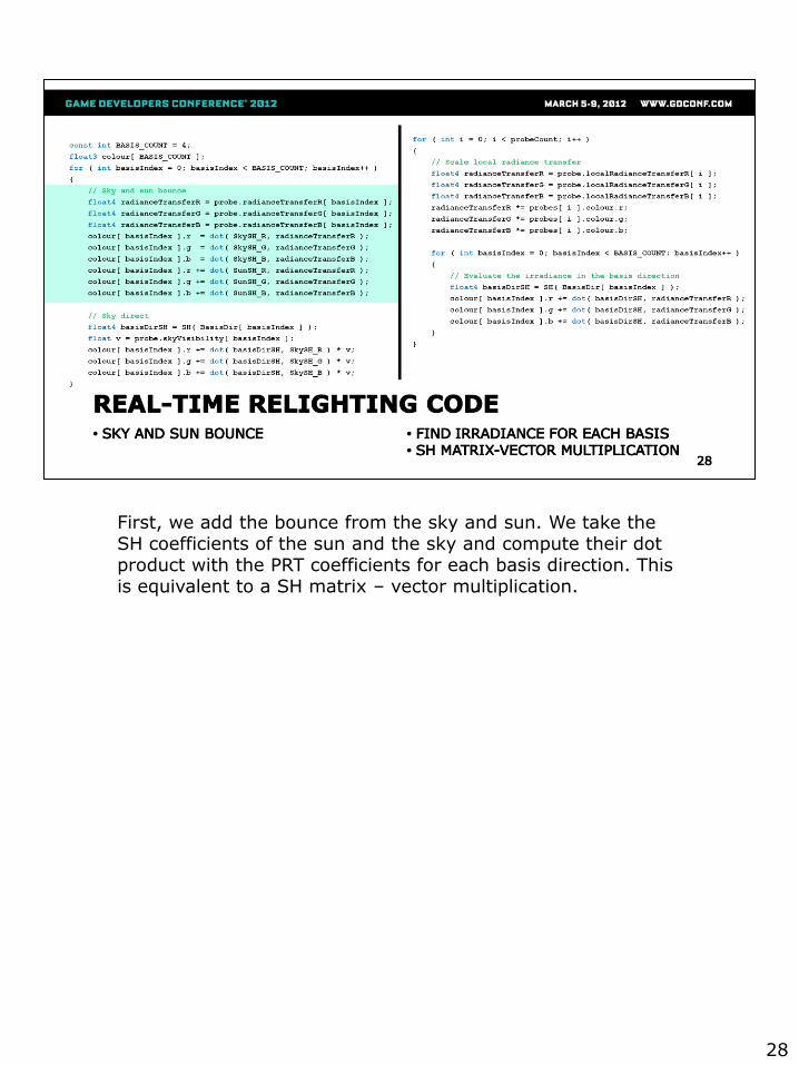
First, we add the bounce from the sky and sun. We take the SH coefficients of the sun and the sky and compute their dot product with the PRT coefficients for each basis direction. This is equivalent to a SH matrix – vector multiplication.

28

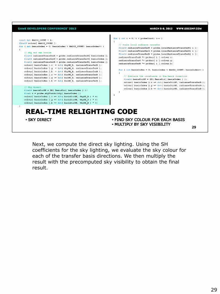
Next, we compute the direct sky lighting. Using the SH coefficients for the sky lighting, we evaluate the sky colour for each of the transfer basis directions. We then multiply the result with the precomputed sky visibility to obtain the final result.

29

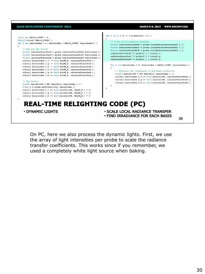
On PC, here we also process the dynamic lights. First, we use the array of light intensities per probe to scale the radiance transfer coefficients. This works since if you remember, we used a completely white light source when baking.

30

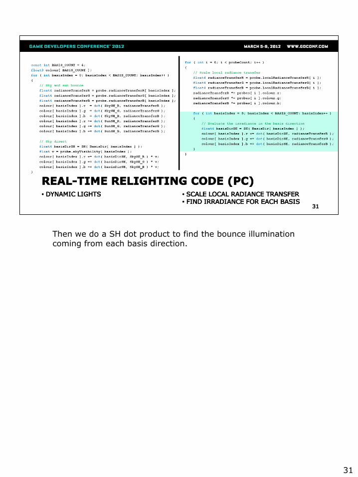
Then we do a SH dot product to find the bounce illumination coming from each basis direction.

31

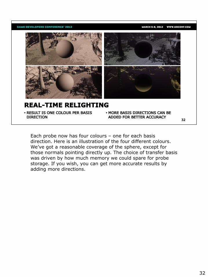
Each probe now has four colours – one for each basis direction. Here is an illustration of the four different colours. We’ve got a reasonable coverage of the sphere, except for those normals pointing directly up. The choice of transfer basis was driven by how much memory we could spare for probe storage. If you wish, you can get more accurate results by adding more directions.

32

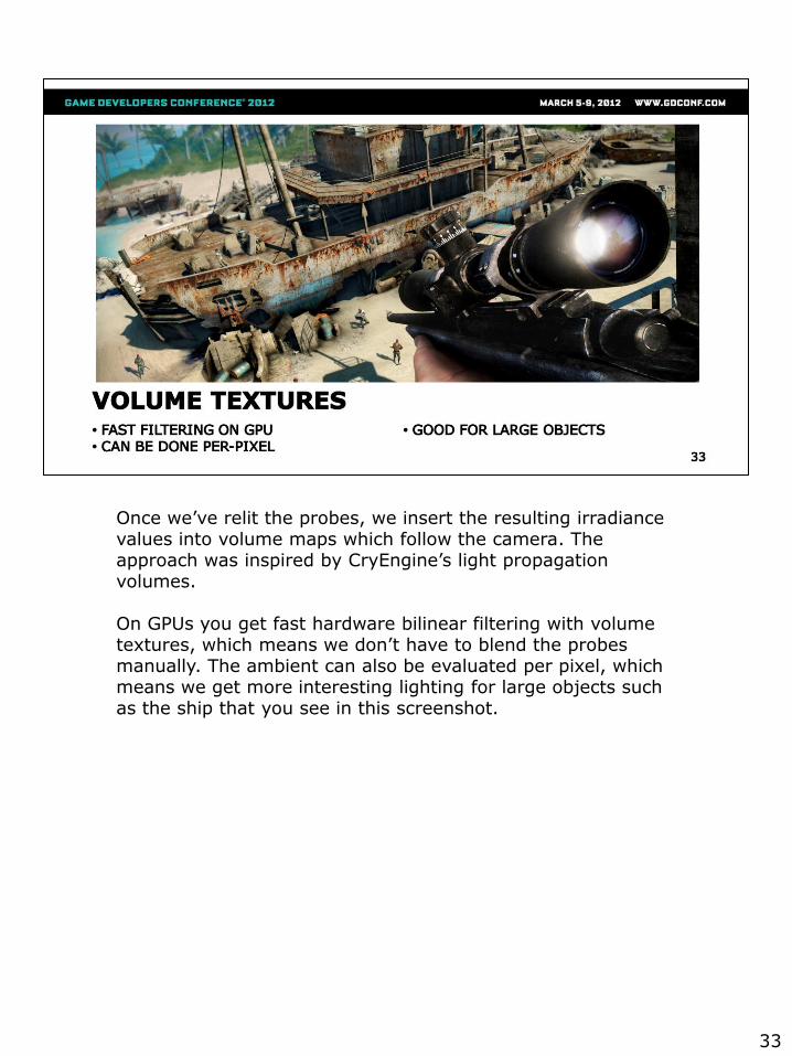
Once we’ve relit the probes, we insert the resulting irradiance values into volume maps which follow the camera. The approach was inspired by CryEngine’s light propagation volumes.

On GPUs you get fast hardware bilinear filtering with volume textures, which means we don’t have to blend the probes manually. The ambient can also be evaluated per pixel, which means we get more interesting lighting for large objects such as the ship that you see in this screenshot.

33

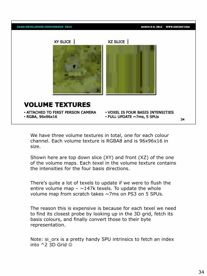
We have three volume textures in total, one for each colour channel. Each volume texture is RGBA8 and is 96x96x16 in size.

Shown here are top down slice (XY) and front (XZ) of the oneof the volume maps. Each texel in the volume texture contains the intensities for the four basis directions.

There’s quite a lot of texels to update if we were to flush the entire volume map – ~147k texels. To update the wholevolume map from scratch takes ~7ms on PS3 on 5 SPUs.

The reason this is expensive is because for each texel we need to find its closest probe by looking up in the 3D grid, fetch its basis colours, and finally convert those to their byte representation.

Note: si_orx is a pretty handy SPU intrinsics to fetch an index into ^2 3D Grid

34

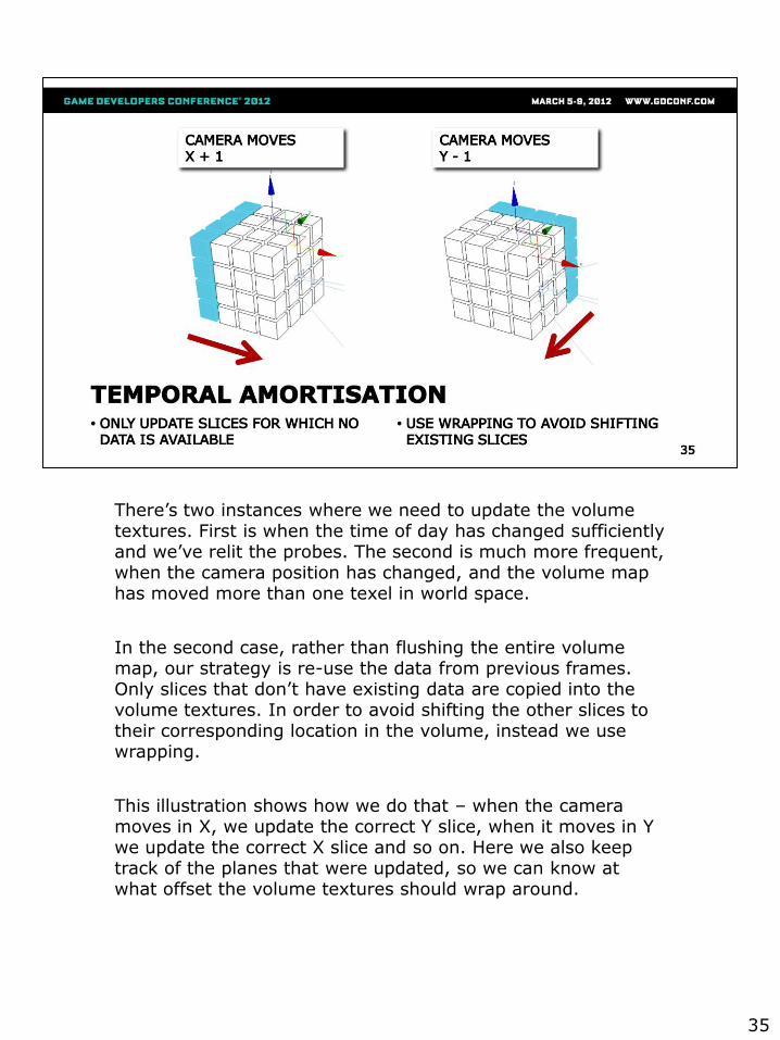
There’s two instances where we need to update the volume textures. First is when the time of day has changed sufficiently and we’ve relit the probes. The second is much more frequent, when the camera position has changed, and the volume map has moved more than one texel in world space.

In the second case, rather than flushing the entire volume map, our strategy is re-use the data from previous frames.Only slices that don’t have existing data are copied into the volume textures. In order to avoid shifting the other slices to their corresponding location in the volume, instead we use wrapping.

This illustration shows how we do that – when the camera moves in X, we update the correct Y slice, when it moves in Y we update the correct X slice and so on. Here we also keep track of the planes that were updated, so we can know at what offset the volume textures should wrap around.

35

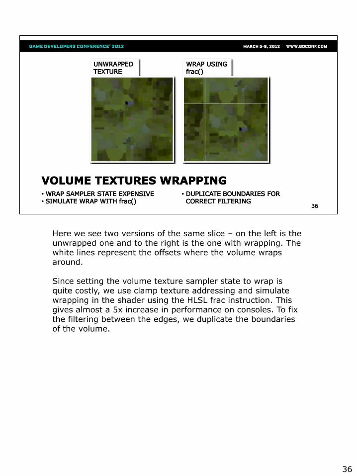
Here we see two versions of the same slice – on the left is the unwrapped one and to the right is the one with wrapping. The white lines represent the offsets where the volume wraps around.

Since setting the volume texture sampler state to wrap is quite costly, we use clamp texture addressing and simulate wrapping in the shader using the HLSL frac instruction. This gives almost a 5x increase in performance on consoles. To fix the filtering between the edges, we duplicate the boundaries of the volume.

36

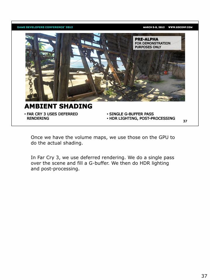
Once we have the volume maps, we use those on the GPU to do the actual shading.

In Far Cry 3, we use deferred rendering. We do a single pass over the scene and fill a G-buffer. We then do HDR lighting and post-processing.

37

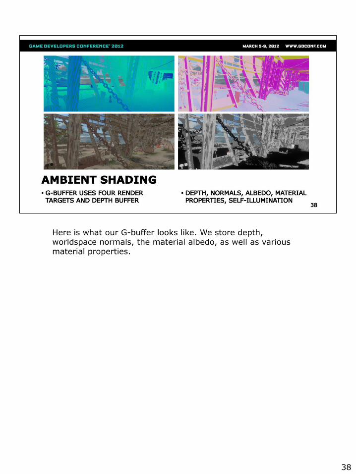
Here is what our G-buffer looks like. We store depth, worldspace normals, the material albedo, as well as various material properties.

38

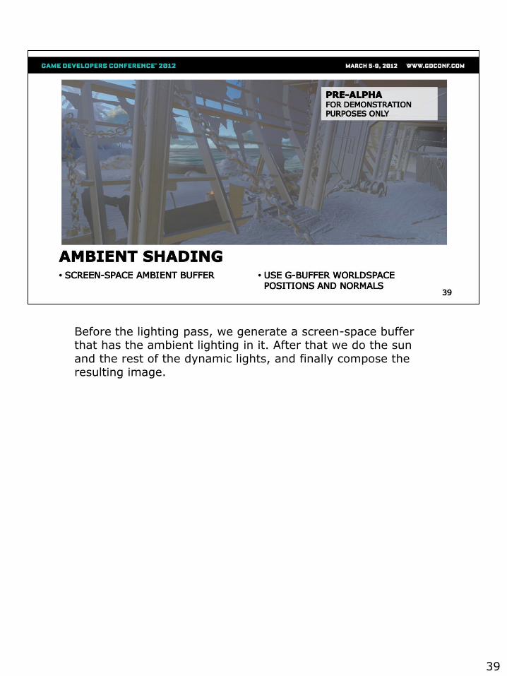
Before the lighting pass, we generate a screen-space buffer that has the ambient lighting in it. After that we do the sun and the rest of the dynamic lights, and finally compose the resulting image.

39

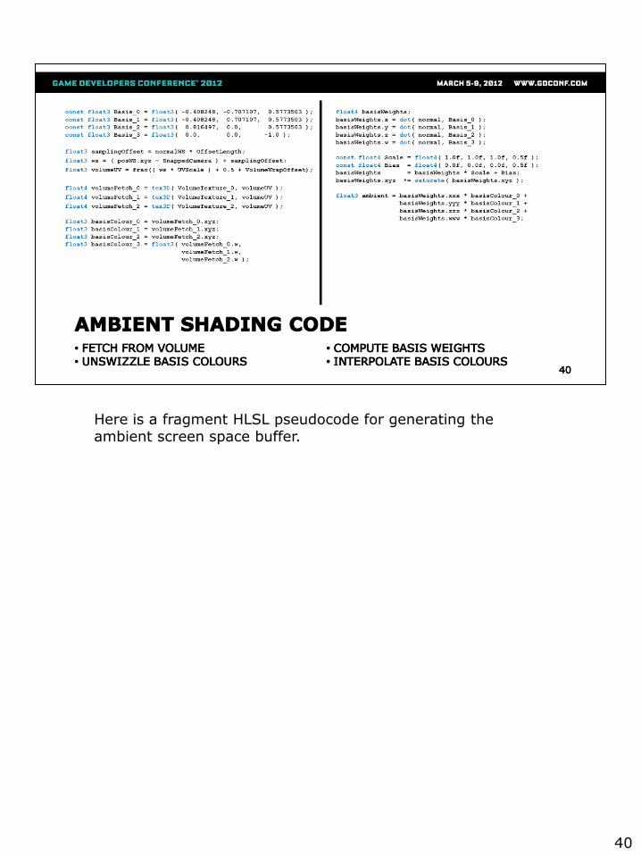
Here is a fragment HLSL pseudocode for generating the ambient screen space buffer.

40

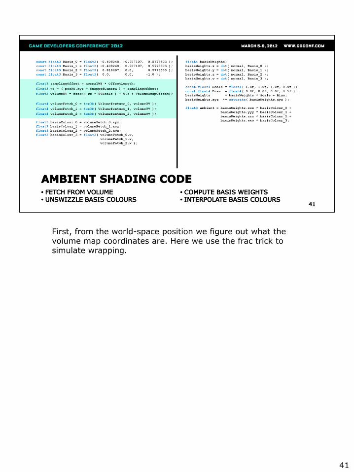
First, from the world-space position we figure out what the volume map coordinates are. Here we use the frac trick to simulate wrapping.

41

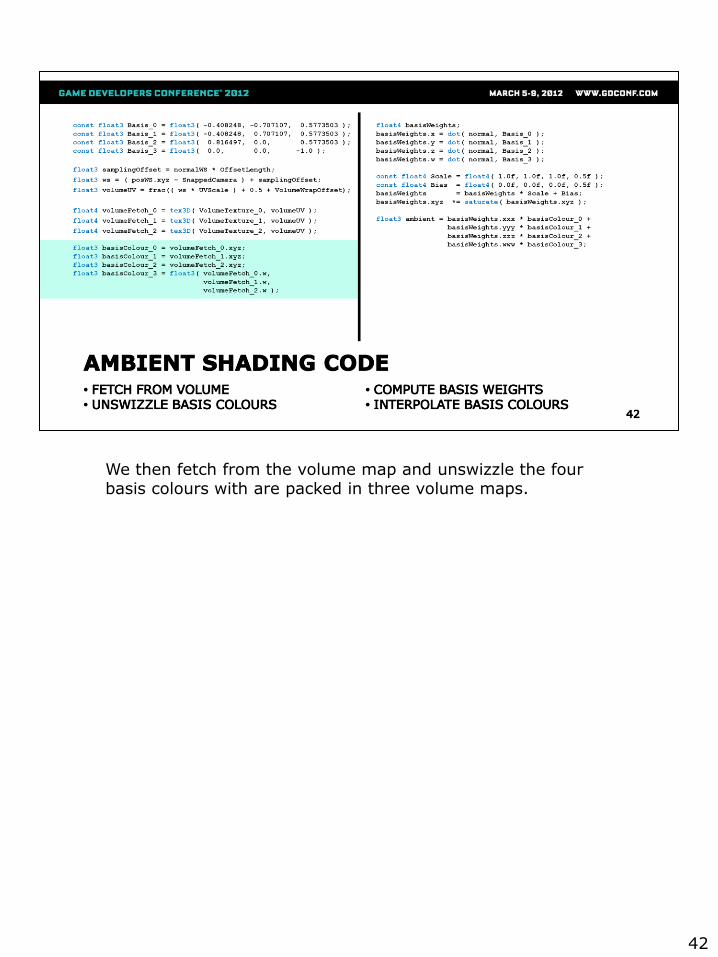
We then fetch from the volume map and unswizzle the four basis colours with are packed in three volume maps.

42

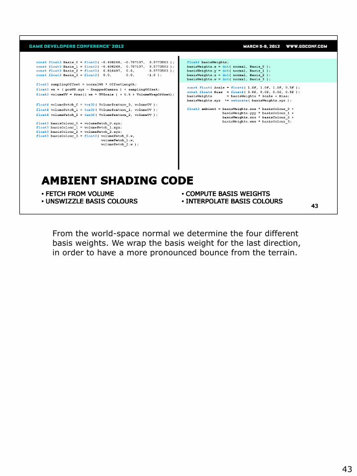
From the world-space normal we determine the four different basis weights. We wrap the basis weight for the last direction, in order to have a more pronounced bounce from the terrain.

43

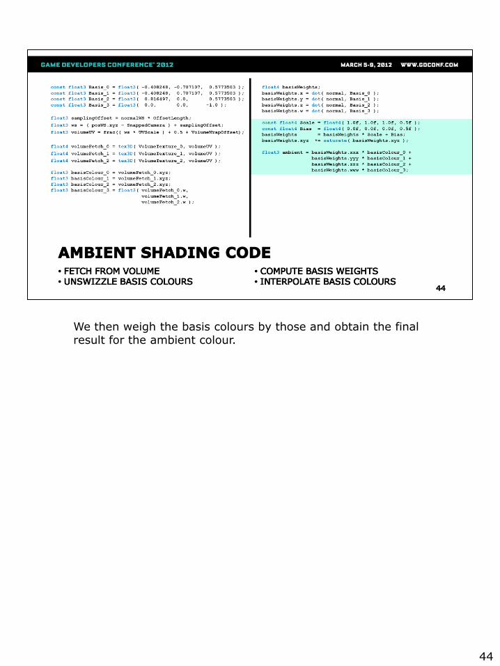
We then weigh the basis colours by those and obtain the final result for the ambient colour.

44

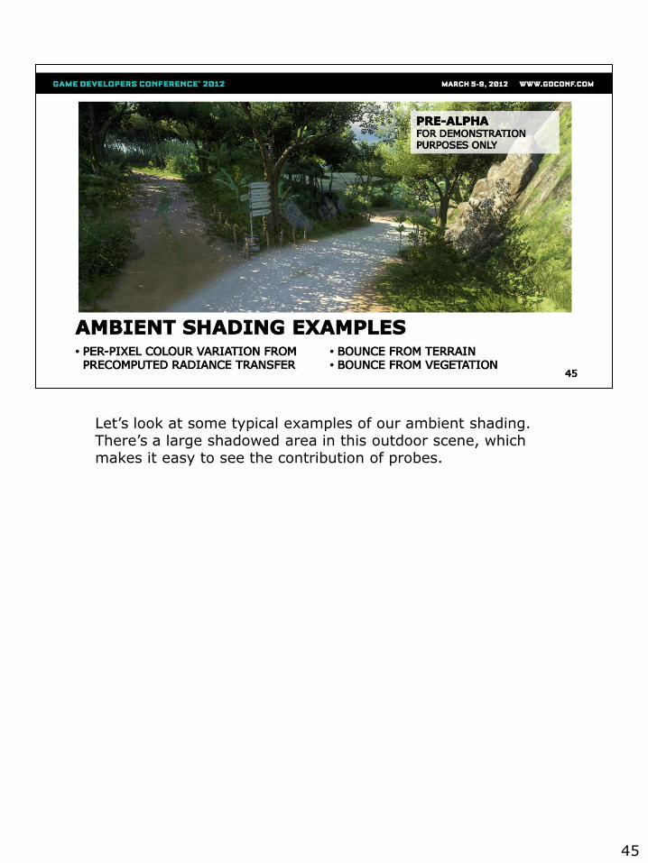
Let’s look at some typical examples of our ambient shading. There’s a large shadowed area in this outdoor scene, which makes it easy to see the contribution of probes.

45

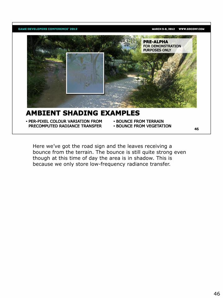
Here we’ve got the road sign and the leaves receiving a bounce from the terrain. The bounce is still quite strong even though at this time of day the area is in shadow. This is because we only store low-frequency radiance transfer.

46

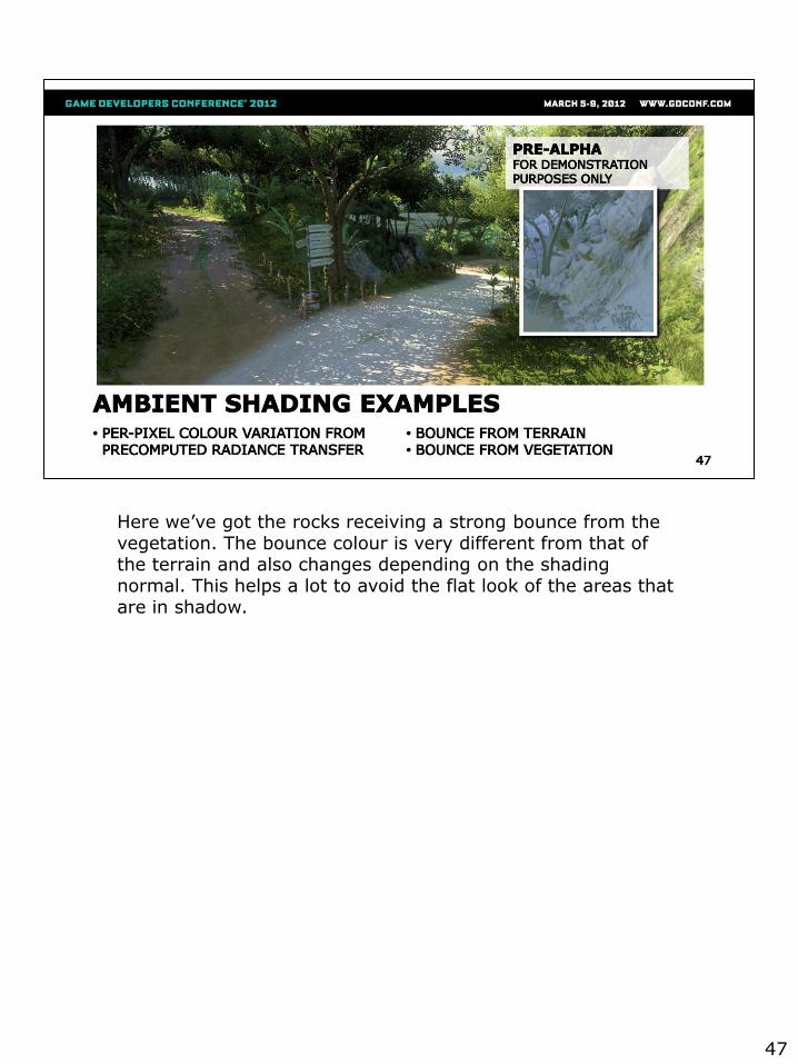
Here we’ve got the rocks receiving a strong bounce from the vegetation. The bounce colour is very different from that of the terrain and also changes depending on the shading normal. This helps a lot to avoid the flat look of the areas that are in shadow.

47

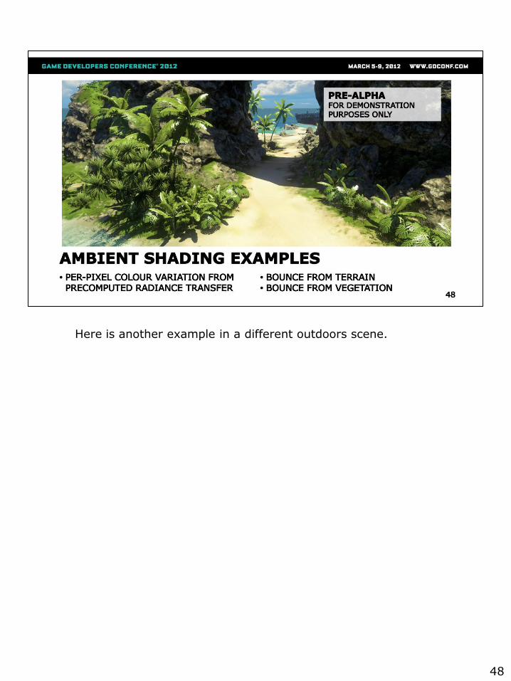
Here is another example in a different outdoors scene.

48

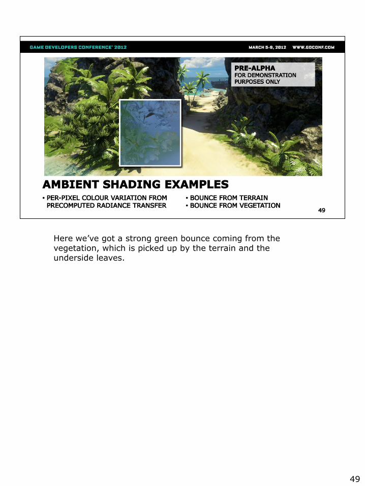
Here we’ve got a strong green bounce coming from the vegetation, which is picked up by the terrain and the underside leaves.

49

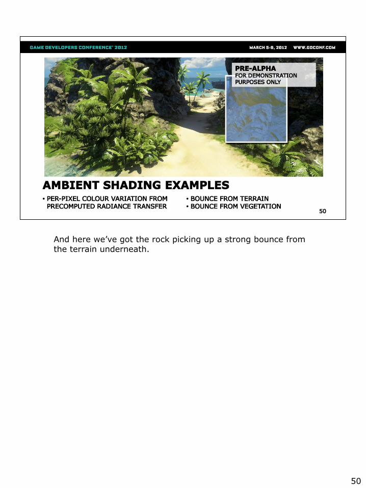
And here we’ve got the rock picking up a strong bounce from the terrain underneath.

50

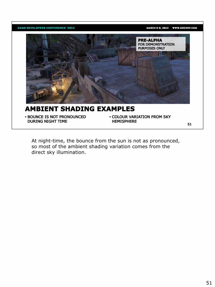
At night-time, the bounce from the sun is not as pronounced, so most of the ambient shading variation comes from the direct sky illumination.

51

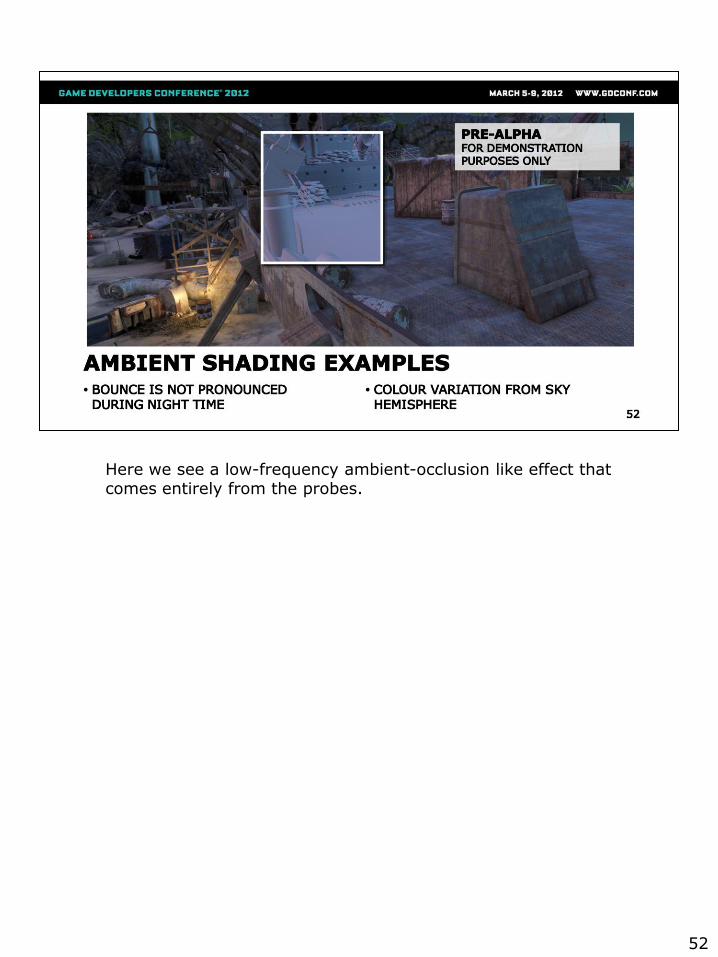
Here we see a low-frequency ambient-occlusion like effect that comes entirely from the probes.

52

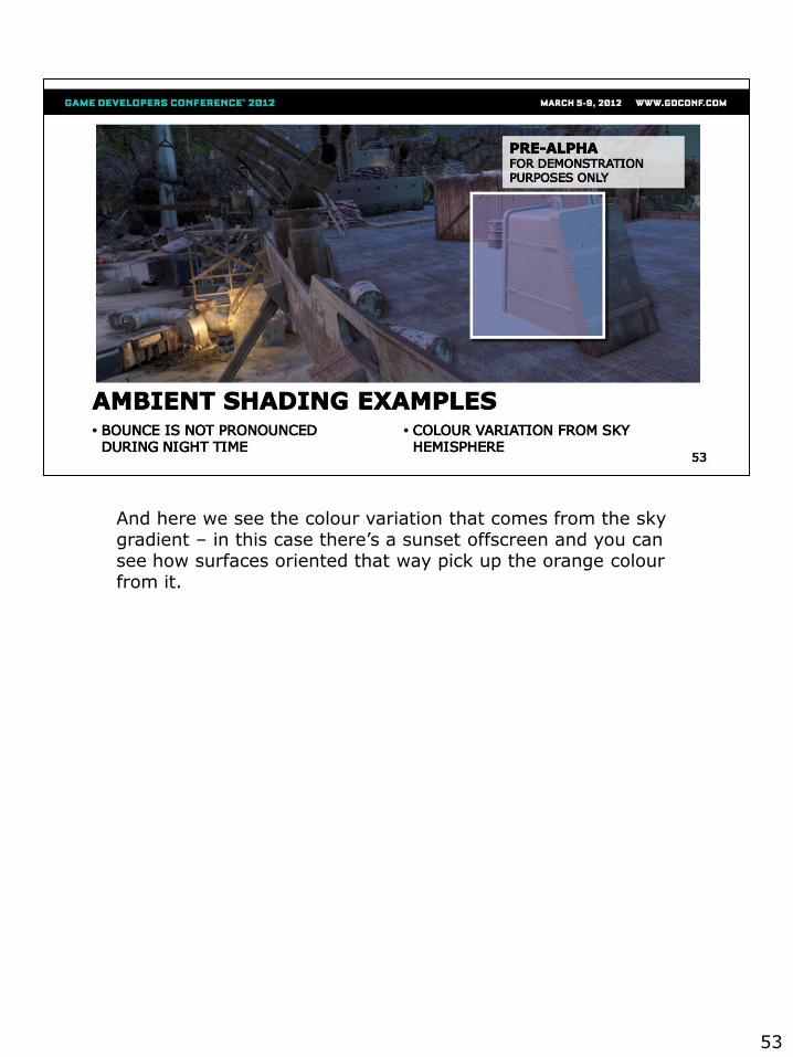
And here we see the colour variation that comes from the sky gradient – in this case there’s a sunset offscreen and you can see how surfaces oriented that way pick up the orange colourfrom it.

53

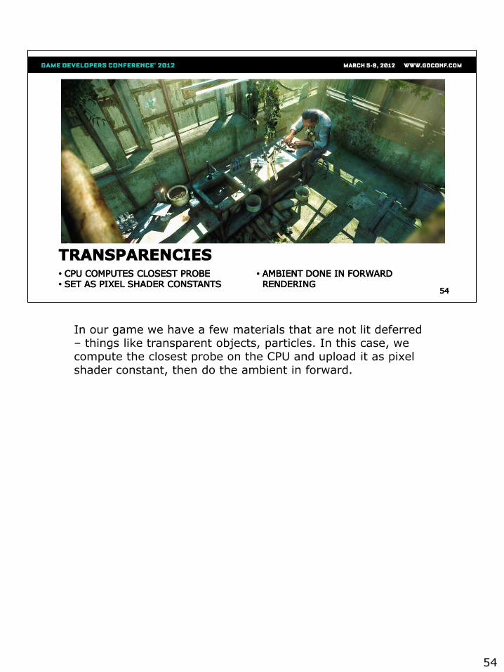
In our game we have a few materials that are not lit deferred – things like transparent objects, particles. In this case, we compute the closest probe on the CPU and upload it as pixel shader constant, then do the ambient in forward.

54

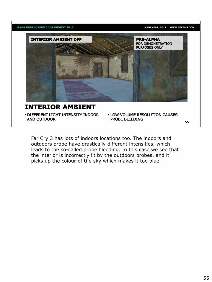
Far Cry 3 has lots of indoors locations too. The indoors and outdoors probe have drastically different intensities, which leads to the so-called probe bleeding. In this case we see that the interior is incorrectly lit by the outdoors probes, and it picks up the colour of the sky which makes it too blue.

55

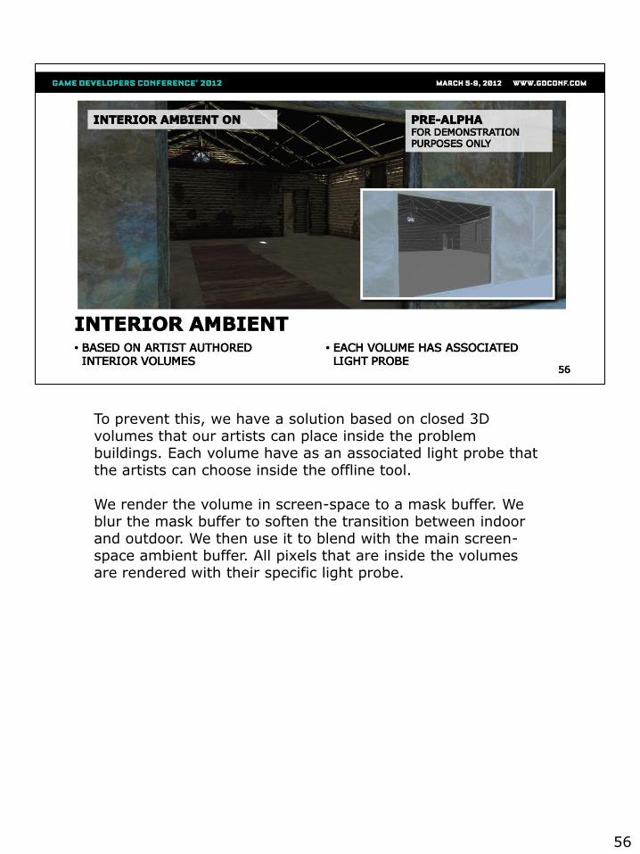
To prevent this, we have a solution based on closed 3D volumes that our artists can place inside the problembuildings. Each volume have as an associated light probe thatthe artists can choose inside the offline tool.

We render the volume in screen-space to a mask buffer. We blur the mask buffer to soften the transition between indoor and outdoor. We then use it to blend with the main screen-space ambient buffer. All pixels that are inside the volumes are rendered with their specific light probe.

56

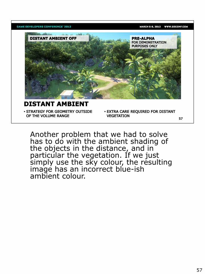
Another problem that we had to solve has to do with the ambient shading of the objects in the distance, and in particular the vegetation. If we just simply use the sky colour, the resulting image has an incorrect blue-ishambient colour.

57

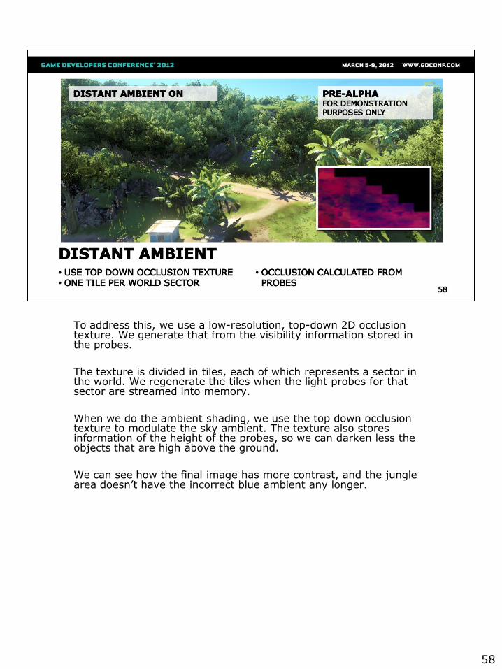
To address this, we use a low-resolution, top-down 2D occlusion texture. We generate that from the visibility information stored in the probes.

The texture is divided in tiles, each of which represents a sector in the world. We regenerate the tiles when the light probes for that sector are streamed into memory.

When we do the ambient shading, we use the top down occlusion texture to modulate the sky ambient. The texture also stores information of the height of the probes, so we can darken less the objects that are high above the ground.

We can see how the final image has more contrast, and the jungle area doesn’t have the incorrect blue ambient any longer.

58

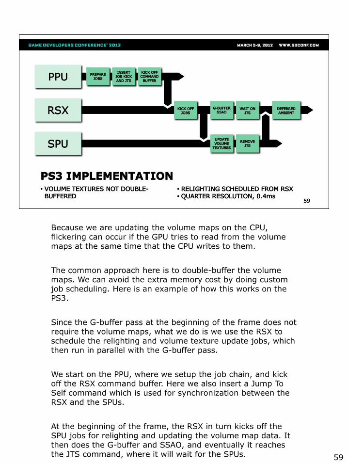
Because we are updating the volume maps on the CPU, flickering can occur if the GPU tries to read from the volume maps at the same time that the CPU writes to them.

The common approach here is to double-buffer the volume maps. We can avoid the extra memory cost by doing custom job scheduling. Here is an example of how this works on the PS3.

Since the G-buffer pass at the beginning of the frame does not require the volume maps, what we do is we use the RSX to schedule the relighting and volume texture update jobs, which then run in parallel with the G-buffer pass.

We start on the PPU, where we setup the job chain, and kick off the RSX command buffer. Here we also insert a Jump To Self command which is used for synchronization between the RSX and the SPUs.

At the beginning of the frame, the RSX in turn kicks off the SPU jobs for relighting and updating the volume map data. It then does the G-buffer and SSAO, and eventually it reaches the JTS command, where it will wait for the SPUs. 59

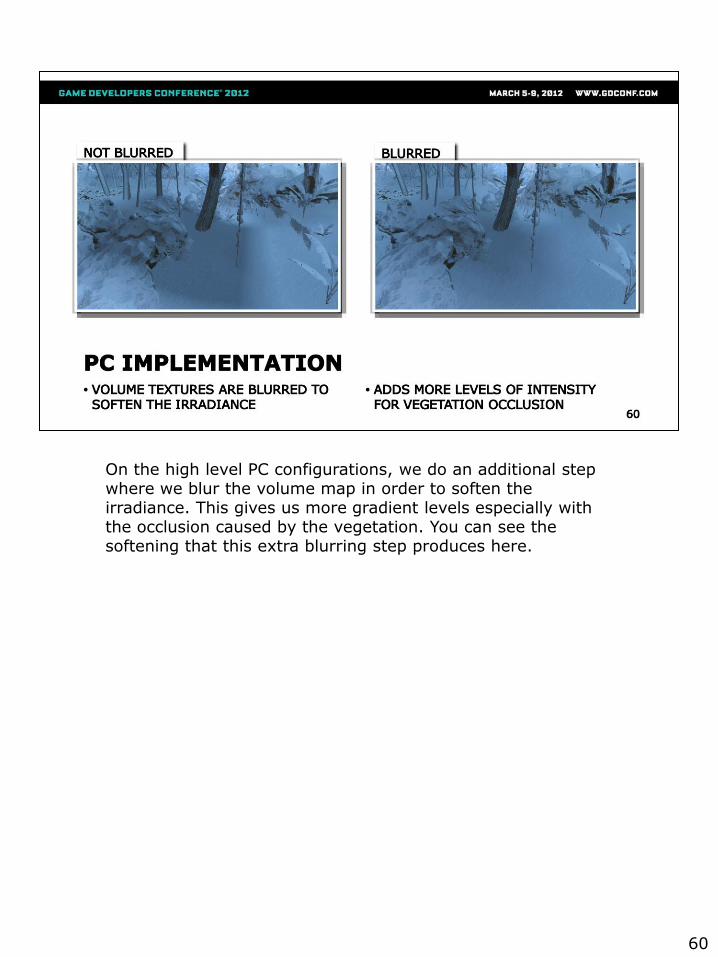
On the high level PC configurations, we do an additional step where we blur the volume map in order to soften the irradiance. This gives us more gradient levels especially with the occlusion caused by the vegetation. You can see the softening that this extra blurring step produces here.

60

Credits

We’d also like to thank the whole FC3 3D Team for their inspirations, and to Stephen Hill, Benjamin Rouveyrol for reviewing the slides and making them more “human readable”

61

Vaas wants you to visit the following websites. Questions?

62

63