Fang, L., Padgett, M. J. and Wang, J. (2017) Sharing a common origin

between the rotational and linear doppler effects. Laser and Photonics

Reviews, 11(6), 1700183. (doi:10.1002/lpor.201700183)

There may be differences between this version and the published version.

You are advised to consult the publisher’s version if you wish to cite from

it.

http://eprints.gla.ac.uk/150757/

Deposited on: 13 November 2017

Enlighten – Research publications by members of the University of Glasgow

http://eprints.gla.ac.uk

brought to you by COREView metadata, citation and similar papers at core.ac.uk

provided by Enlighten

1

Original Paper

Sharing a common origin between the rotational and linear Doppler effects

Liang Fang1, Miles J. Padgett2, and Jian Wang1*

*Corresponding Author: E-mail: jwang@hust.edu.cn

1Wuhan National Laboratory for Optoelectronics, School of Optical and Electronic

Information, Huazhong University of Science and Technology, Wuhan 430074, Hubei, China. 2 School of Physics and Astronomy, University of Glasgow, Glasgow G12 8QQ, Scotland,

UK

Abstract: The well-known linear Doppler effect arises from the linear motion between source

and observer, while the less well-known rotational Doppler effect arises from the rotational

motion. Here, we present both theories and experiments illustrating the relationship between

the rotational and linear Doppler effects. A spiral phaseplate is used to generate a light beam

carrying orbital angular momentum and the frequency shift is measured arising from its

rotational and/or linear motion. By considering either the motion-induced time-evolving phase

or the momentum and energy conservation in light-matter interactions, we derive the

rotational Doppler shift, linear Doppler shift, and overall Doppler shift associated with

rotational and linear motions. We demonstrate the relationship between rotational and linear

Doppler shifts, either of which can be derived from the other effect, thereby illustrating their

shared origin. Moreover, the close relationship between rotational and linear Doppler effects

is also deduced for a more general moving rough surface.

1. Introduction

The Doppler effect is the change in frequency of a wave that arises from the relative motion

between a source and an observer. The Austrian physicist Doppler first proposed this effect in

1842 [1] and Ballot tested the hypothesis for sound waves in 1845 [2] and Fizeau discovered

independently the same phenomenon with electromagnetic waves in 1848 [3]. The Doppler

2

shift arising from either sound waves or electromagnetic waves back-scattered from a moving

object is used in sonar and radar systems for velocity measurements. The classical Doppler

effect, arising from the linear motion or linear momentum, is also called the linear Doppler

effect and has been used extensively in various fields as diverse as laser interferometers, laser

remote sensing, laser speckle velocimetry, and astronomy [4-8].

Less well known than this linear Doppler effect is the rotational Doppler effect, which arises

from rotational motion and optical angular momentum [9-15]. A simple example of this

phenomenon is obtained by placing a watch at the center of a rotating turntable and, as viewed

from above, the hands of the watch rotate more quickly than normal [16]. This effect applies

not just to watch hands but to all rotating vectors, and the rotating electric-field vector of

circularly polarized light, that carries spin angular momentum, is no exception. The electric-

field vector rotates at the light frequency, while an additional rotation of the light around its

propagation axis can speed up or slow down the rotation of the electric-field vector, leading to

a frequency shift linked to the rotational velocity. Note, this rotational Doppler effect can be

observed by looking at a rotating body in a direction parallel to its rotation axis, the direction

in which the linear shift is zero. This rotational effect is distinct from the linear Doppler effect

observed from viewing the edges of a rotating extended body (e.g. galaxy) in a direction

perpendicular to its rotation axis.

More generally, the angular momentum of light can be divided into spin angular momentum

(SAM) and orbital angular momentum (OAM). The SAM arises from the circular polarization

of light and gives two possible values equivalent to h per photon (where is the Plank’s

constant h divided by 2 ), as anticipated by Poynting in 1909 [17]. By contrast, the OAM

arises from helical phase fronts described by exp i l (where l is the topological charge and

is the azimuthal angle). Unlike the SAM that is restricted to two orthogonal states, the

OAM is restricted only by the aperture of the optical system and has a value of l h per photon,

3

as recognized by Allen in 1992 [18]. OAM has given rise to many developments in particle

manipulation, microscopy, imaging, sensing, astronomy and both quantum and classical

communications [19-29]. Recently, OAM-carrying light has also been studied in relation to

the rotational Doppler effect, allowing detection of spinning objects, measurement of fluid

flow vorticity, and effects in nonlinear optics [30-38].

In this paper, we consider whether the rotational Doppler effect and linear Doppler effect

share a common origin, unlike for example the relativistic transverse Doppler effect which is

related to time dilation. By employing a spiral phaseplate and exploiting OAM-carrying light,

we illustrate the relationship between rotational and linear Doppler effects, i.e. show how

either frequency shift can be alternatively explained both in terms of the rotational or linear

Doppler effect.

2. Concept and Theory

2.1. Spiral Phaseplate

A natural way of generating light beams containing OAM is by transmission of a plane-wave

Gaussian beam through a spiral phaseplate [39]. A spiral phaseplate is simply a transmissive

disc with an optical thickness, H , that increases with azimuthal angle, (2 )H l , where

is the wavelength of light. Instead of transmission, as shown in Fig. 1, the same concept

can be also applied in reflection where an incident plane wave is reflected from a helical

surface with a step height of 2 (2 ) (4 )H l l , giving a reflected light beam with a

helical phase front described by exp i l , and hence an OAM of l h per photon. The factor of

two reduction in step height between the two equations when moving from transmission to

reflection is to account for the double pass associated with the reflection. As an alternative to

a physical implementation, these spiral phaseplates can be implemented using the spatially

4

dependent geometrical phase associated with transmission through liquid crystal [40] or

metamaterials [41], or encoded directly onto a spatial light modulator (SLM) [19, 20, 42].

2.2 Rotational Doppler Effect

As shown in Fig. 1(a), if the spiral phaseplate is rotated through an angle around its

central axis then the reflected light acquires a phase shift of l . If this rotation is

continuous, with rotational velocity /d dt , then the resulting time-evolving phase is

manifest as a frequency shift in the reflected light of = / / (2 ) / (2 )f d dt , a form of the

rotational Doppler shift.

This rotational Doppler shift can also be understood from the conservation of the angular

momentum and energy in the light-matter interaction [43]. Upon reflection the light has a

change in its angular momentum of l h per photon. Accordingly, the conservation of angular

momentum dictates that the rotating spiral phaseplate experiences an opposite impulse torque

of l h per photon. The spiral phaseplate rotating at rotational velocity does work against

this torque delivering an energy to the reflected light of E l h per photon, leading to a

frequency shift of = / / (2 )f E h , i.e. the rotational Doppler shift.

2.3 Linear Doppler Effect

The linear Doppler shift is also understandable based on similar conservations of linear

momentum and energy in the light-matter interaction. A single photon reflected from the

surface undergoes a change in its linear momentum of 2kh , with the mirror being subject to

an equal but opposite impulse, where 2 / 2 /k f c is the wavenumber, f is the

frequency of light, and c the light velocity. If the mirror is moving at linear velocity , this

impulse corresponds to an energy transfer per photon in the reflected light of 2E kv h .

Equating this energy transfer to the change in optical frequency gives a frequency shift of

= / 2 /f E h fv c , i.e. the linear Doppler shift (Note that in this case the factor of two arises

5

because the light is Doppler shifted once at the surface and then Doppler shifted a second time

as it is received from this moving surface back at the source).

2.4 Linking the Rotational and Linear Doppler Effects

In the case of the spiral phaseplate, the rotational frequency shift can also be alternatively

derived from the linear Doppler effect. As shown in Fig. 1(b), the back reflection from a

planar mirror moving with respect to the source with a linear velocity v , creates a time-

evolving phase of 2kvt , resulting in a linear Doppler shift given by = (2 ) / / (2 ) 2 /f d kvt dt fv c

as above. The rotation of the spiral phaseplate also creates a movement of its helical surface

towards or away from the source/observer. For a step height of 2l and a rotational velocity

of , shown in Fig. 1(a), any location on the helical surface of the phaseplate has a linear

velocity with respect to the source of = [( / 2) / (2 )] / = / (4 ) / / (4 )d dt d dt . This

linear velocity gives an observed frequency shift of =2 / =2 / (4 ) /f f c f c , or simply

= / (2 )f , i.e. identical to that derived from the rotational Doppler shift. Consequently,

here is an example where a frequency shift can be equivalently explained either in terms of

the rotational Doppler effect or linear Doppler effect, illustrating, at least in this case, their

common origin.

Remarkably, it is well known that, the rotational Doppler shift = / (2 )f is frequency

independent, while the linear Doppler shift =2 /f fv c is dependent on the frequency of light,

giving a false impression of their conflict in the shared common orgin. Actually, when

deducing the rotational Doppler shift based on the linear Doppler effect, the equivalent linear

velocity = / (4 ) of any location on the helical surface of the rotating spiral phaseplate

( ) is also frequency (wavelength) dependent. As a result, the frequency dependence in the

linear Doppler shift is removed in the deduced rotational Doppler shift.

6

The rotational Doppler effect can be deduced from the linear Doppler effect in the case of the

spiral phaseplate and vice versa. The linear motion ( v ) of the spiral phaseplate, causing a

phase change, is also equivalent to its rotational motion ( 4 / ( )v ) producing the same

amout of the phase variation. Hence, the linear Doppler shift can also be alternatively derived

from the rotational Doppler effect.

2.5 Overall Doppler Shift

When the spiral phaseplate is subject to simultaneous rotational motion and linear motion, as

shown in Fig. 1(c), a total frequency shift can also be deduced. The incident plane wave is

transformed into an OAM-carrying light beam by the spiral phaseplate, meaning that the

reflected light undergoes a change in its angular momentum of l h per photon and additionally

the reflection results in a change in its linear momentum of 2kh . Hence, the moving spiral

phaseplate experiences both a impulse torque of l h and radiation pressure impulse of 2kh per

photon. Therefore moving the spiral phaseplate with rotational velocity against this

impulse torque and with linear velocity v against this radiation pressure, produces a total

energy transfer to the reflected light of ( 2 )E kv per photon, resulting in a frequency

shift of = / / (2 ) 2 /f E h f c . The overall Doppler shift is therefore the sum of both the

rotational Doppler shift ( / (2 ) ) and the linear Doppler shift ( 2 /fv c ). By linking the

rotational and linear Doppler effects, we can simply obtain the same results of equivalent

rotational or linear Doppler shift irrespective of the approach taken to their individual

calculation (see Supporting Information).

It is clear that the rotational Doppler effect and linear Doppler effect have close relationship.

The overall Doppler shift and the relationship between rotational Doppler shift and linear

Doppler shift can be also deduced by considering the moving spiral phaseplate along the

angular direction as a triangular wedge in polar coordinates (see Supporting Information).

7

Figure1 Illustration of rotational Doppler effect, linear Doppler effect and overall

Doppler effect. (a) A spiral phaseplate rotating around the optical axis gives rise to the

rotational Doppler shift. (b) A mirror translating along the optical axis gives rise to the linear

Doppler shift. (c) A moving spiral phaseplate with simultaneous rotational motion and linear

motion gives rise to the overall Doppler shift (rotational Doppler shift and linear Doppler

shift). Both of these shifts can be understood in terms of the linear Doppler shift albeit the

rotational case is a specific example of a general rotational Doppler shift.

3. Experimental Realization

3.1 Experimental Configuration

To verify the link between the rotational and linear Doppler effects, we setup an experimental

configuration, as shown in Fig. 2(a). The configuration can be regarded as a modified Mach-

Zehnder interferometer with the scanning mirror replaced with the moving spiral phaseplate.

An SLM loaded with a time-varying spiral phase mask is employed to emulate the moving

spiral phaseplate (see Supporting Information). A He-Ne laser emitting at 632.8 nm is divided

into two optical paths by a non-polarizing beam splitter (BS). One path is used as a reference

Gaussian light beam with its power and beam size adjusted by a neutral density filter (NDF)

and a lens, respectively. The other path is reflected from the time-varying spiral phase mask

through a mirror and a second BS. A polarizer (Pol.) and a half-wave plate (HWP) after the

laser are used to set the polarization state of the light to match the required polarization of the

polarization-dependent SLM. The OAM-carrying light beam reflected from the spiral phase

8

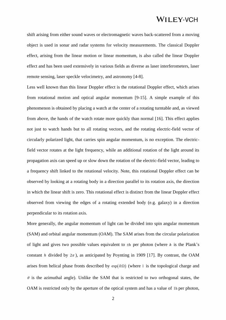
mask encoded on the SLM is reflected by the second BS and then combined with the

reference Gaussian light beam using a further BS together to produce the characteristic helical

interference fringes [44]. Another lens followed by a camera enables an image of the helical

interference fringe pattern to be recorded, as shown in Fig. 2(b), from which the sign and

magnitude of the OAM is confirmed and, from the rotation of the fringes, the Doppler

frequency shift is deduced (see Supporting Information).

Figure 2 Experimental configuration and helical interference fringes. (a) Experimental

configuration of a modified Mach-Zehnder interferometer for the measurement of rotational

and linear Doppler effects. The rotational motion and linear motion of the spiral phaseplate

are emulated by employing a spatial light modulator (SLM) loaded with a time-varying spiral

phase mask. Pol.: polarizer; HWP: half-wave plate; BS: beam splitter; NDF: neutral density

filter. (b) Measured helical interference fringes (interference between an OAM-carrying light

beam and a reference Gaussian light beam). The twist number and twist direction of the

helical interference fringes are determined by the magnitude and sign of the OAM, and their

rotation is a manifestation of the frequency shift.

3.2 Results and Discussions

To highlight the equivalence of rotational Doppler shift and linear Doppler shift, we measure

the frequency shift arising from separate rotational motion and linear motion. To confirm the

9

derived relationship of = / (4 ) or 4 / ( ) , we choose two initial cases where case 1

is the rotational only motion ( 500 rad/s, 0v ) and case 2 is the linear only motion ( =0 ,

76v μm/s).

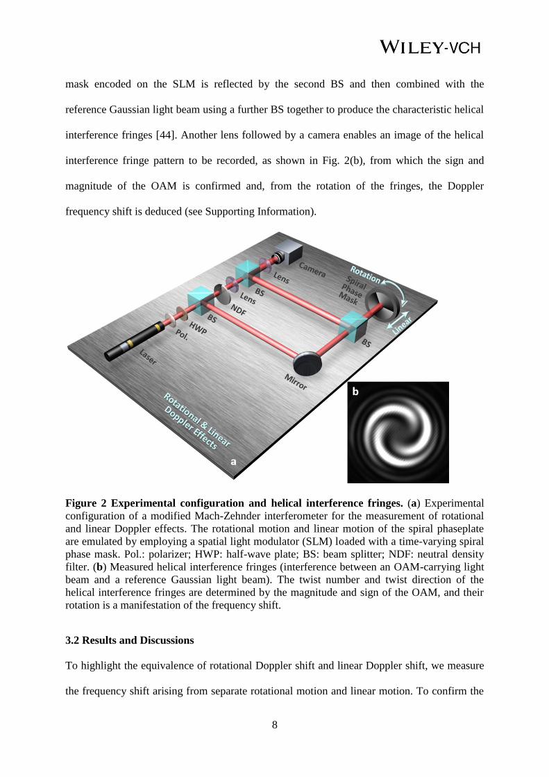
As a representative OAM-carrying light beam we report the results for l =3 and in both cases

obtained by measuring the time-varying intensity at an off-axis position in the helical

interference fringes. The recorded time-varying intensity and its Fourier-transformed

frequency spectra for two cases are shown in Fig. 3. One can see clearly that the measured

rotational Doppler shift of 241 Hzf is almost identical to the measured linear Doppler shift

of 240 Hzf . Thereby, unsurprisingly, the same frequency shift can be produced by either

rotational or linear Doppler effect.

Figure 3 Time-varying intensity and Doppler frequency shift. (a), (c) Measured time-

varying intensities at an off-axis position in the helical interference fringes. (b), (d) Fourier-

transformed frequency spectra. (a), (b) Case 1: rotational only motion ( =500 rad/s, 0v )

with measured frequency shift of 241 Hzf . (c), (d) Case 2: linear only motion ( =0 , 76v

μm/s) with measured frequency shift of 240 Hzf . The OAM value is l =3.

To further compare the rotational and linear Doppler shifts and show their close relationship,

we employ different OAM values of l =1, 3, 5 and different rotational and linear velocities.

Shown in Fig. 4 is the measured frequency shift as a function of the rotational velocity or

linear velocity. It is clearly shown that the f v curve is independent on OAM values while,

10

as expected, different OAM values give different slopes of f curves. The larger the

OAM value, the larger the slope of the f curve. Shown in the inset of Fig. 4 are -v

curves indicating the relationship between linear velocity and rotational velocity

( = / (4 ) l ) required to give the same Doppler frequency shift. Consequently, the same

frequency shift can be generated from either the rotational Doppler effect or the linear

Doppler effect.

Figure 4 Rotational and linear Doppler shifts. Measured frequency shift versus rotational

velocity ( ) or linear velocity ( v ). -f v curve is independent on OAM values. Different

OAM values give different slopes of -f curves. The inset shows -v curves. Markers:

experimental results; solid lines: theories ( / (2 )f l , =2 /f f c , = / (4 ) l ).

For the overall Doppler shift arising from simultaneous rotational motion and linear motion

shown in Figs. 5(a) and 5(d), following the relationship of = / (4 ) or 4 / ( )

between the rotational velocity and linear velocity, we also show its equivalent linear Doppler

shift with linear only motion shown in Figs. 5(b) and 5(e) and equivalent rotational Doppler

shift with rotational only motion shown in Figs. 5(c) and 5(f).

11

Figure 5 | (a)-(f) Overall Doppler shift and its equivalent rotational and linear Doppler

shift. (g)-(l) Overall Doppler shift close to zero. (a) Measured overall Doppler shift versus

rotational velocity ( ) and linear velocity ( v ) for simultaneous rotational motion and linear

motion. (b) Measured equivalent rotational Doppler shift versus rotational velocity ( ) for

rotational only motion. (c) Measured equivalent linear Doppler shift versus linear velocity ( v )

for linear only motion. (d), (e), (f) Measured time-varying intensities at an off-axis position in

the helical interference fringes (upper row) and Fourier-transformed frequency spectra (lower

row) corresponding to the middle point in (a), (b), (c). (g) Measured rotational Doppler shift

versus rotational velocity ( ) for rotational only motion. (h) Measured linear Doppler shift

versus linear velocity ( v ) for linear only motion. (i) Measured overall Doppler shift close to

zero for simultaneous rotational motion and linear motion satisfying the relationship of v -

/ (4 ) . (j), (k), (l) Measured time-varying intensities at an off-axis position in the helical

interference fringes (upper row) and Fourier-transformed frequency spectra (lower row)

corresponding to the middle point in (g), (h), (i). The OAM value is l =3. Markers:

experimental results; solid lines: theories ((a), (i) 2 / / (2 )f f c , (b), (g) / (2 )f ,

(c), (h) 2 /f fv c ).

12

Obviously, the rotational Doppler shift and the linear Doppler shift can also cancel with each

other, resulting in an overall Doppler shift close to zero, as shown in Figs. 5(g)-5(l). Although

separate rotational/linear only motion is detectable from its corresponding rotational/linear

Doppler shift shown in Figs. 5(g), 5(h), 5(j) and 5(k), the overall motion is undetectable when

the rotational velocity and linear velocity satisfy the relationship of = - / (4 ) , as shown

in Figs. 5(i) and 5(l).

The measured data in the proof-of-concept experiment shown in Figs. 3-5 are in good

agreement with the theories. The maximum relative error of the measurement is less than 5%.

The obtained results show successful demostration of the close relationship between rotational

and linear Doppler effects. High precision measurement is achieved in the experiment when

using SLM as an alternative to the physical implementation of a spiral phaseplate (see

Supporting Information).

4. General Rough Surface

More generally, we consider the equivalent relationship between the rotational and linear

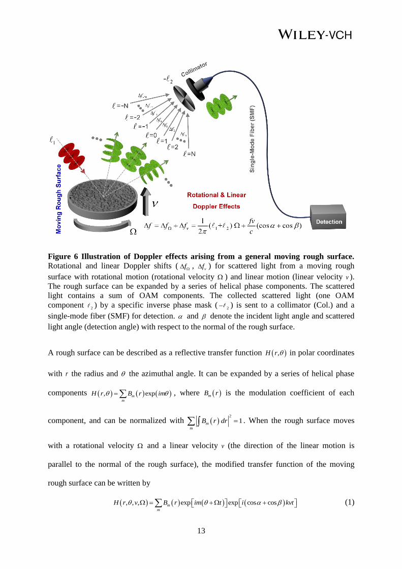
Doppler effects for scattered light from a moving rough surface. As illustrated in Fig. 6, the

incident light beam is scattered by a moving rough surface with simultaneous rotational

motion and linear motion. The scattered light can be decomposed into a sum of different

OAM components. A specific inverse spiral phase mask can be used to collect the desired

OAM component and convert it into a Gaussian-like light beam with a bright spot at the beam

center. The collected scattered light is then sent to a collimator (Col.) followed by a single-

mode fiber (SMF) for spatial filtering and detection.

13

Figure 6 Illustration of Doppler effects arising from a general moving rough surface.

Rotational and linear Doppler shifts ( f , vf ) for scattered light from a moving rough

surface with rotational motion (rotational velocity ) and linear motion (linear velocity v ).

The rough surface can be expanded by a series of helical phase components. The scattered

light contains a sum of OAM components. The collected scattered light (one OAM

component 2) by a specific inverse phase mask (

2 ) is sent to a collimator (Col.) and a

single-mode fiber (SMF) for detection. and denote the incident light angle and scattered

light angle (detection angle) with respect to the normal of the rough surface.

A rough surface can be described as a reflective transfer function ,H r in polar coordinates

with r the radius and the azimuthal angle. It can be expanded by a series of helical phase

components , expm

m

H r B r im , where mB r is the modulation coefficient of each

component, and can be normalized with 2

1m

m

B r dr . When the rough surface moves

with a rotational velocity and a linear velocity v (the direction of the linear motion is

parallel to the normal of the rough surface), the modified transfer function of the moving

rough surface can be written by

, , , exp exp cos cosm

m

H r v B r im t i kvt (1)

14

where k is the wavenumber, and indicate the incident light angle and scattered light

angle (detection angle) with respect to the normal of the rough surface, respectively. When

facing the rough surface, the sign (+/-) of and v , denotes the clockwise/counterclockwise

rotational motion and forward/backward linear motion, respectively.

The electric field of an incident light beam, carrying an OAM of 1 at a frequency f , is

given by

11 1, , exp 2E r t C i ft (2)

where 1

C is related to the transverse electric field distribution of the OAM-carrying light

beam and the wavenumber k and propagation distance z related phase term is not given here.

The scattered light from the moving rough surface can be expressed as

1

2 1

1

, , , , , - , , , ,

exp exp 2 (cos cos )m

m

E r v t E r t H r v

B C i m i f m kv t

(3)

It clearly shows that for the scattered light, different OAM (2 1m ) components have

different overall Doppler frequency shifts, generally written by

1(cos cos )

2v

fvf f f m

c

(4)

For separate rotational only motion, the corresponding rotational Doppler shift is expressed as

1

2f m

(5)

For separate linear only motion, the corresponding linear Doppler shift is expressed as

(cos cos )v

fvf

c (6)

For the rotational motion with a rotational velocity of , the resultant rotational Doppler shift

can be also understood from the same amount of linear Doppler shift by a linear motion with

the corresponding linear velocity v written by

15

1

2 cos cos

mv

(7)

Similarly, for the linear motion with a linear velocity of v , the resultant linear Doppler shift

can be also understood from the same amount of rotational Doppler shift by a rotational

motion with the corresponding rotational velocity written by

2(cos cos )

v

m

(8)

For the OAM component 2 1 ( m 0) in the scattered light, it is clear from Eqs. (4) and (5)

that there is no rotational Doppler shift, which is analogous to the case of no rotational

Doppler shift for mirror reflection with an incident OAM beam.

We consider two more special cases of Doppler shift for scattered light from a moving rough

surface: 1) the incident light beam is a plane wave while the collected scattered light

component carries an OAM ( ℓ¹ 0); 2) the incident light beam carries an OAM ( ℓ¹ 0) while

the collected scattered light component is a plane wave. The former is corresponding to the

aforementioned spiral phaseplate case, while the latter interchanges the source and observer.

In general, the incident angle and scattered angle may take moderate values. When

assuming small incident and scattered angles for both two cases ( 0 ,

2 2cos 1 2sin 2 1 2 1 , 2 2cos 1 2sin 2 1 2 1 ), the overall Doppler shift

expressed in Eq. (4) can be simplified as / (2 ) 2 /f fv c . Accordingly, the rotational

Doppler shift for separate rotational only motion is / (2 )f , and the linear Doppler shift

for separate linear only motion is 2 /vf fv c . The rotational Doppler shift under a rotational

velocity of is also understandable from the linear Doppler shift under an equivalent linear

velocity / (4 )v . The linear Doppler shift under a linear velocity of v is also

understandable from the rotational Doppler shift under an equivalent rotational velocity

16

4 / ( )v . These show exactly the same results as obtained above for a moving spiral

phaseplate or its equivalent physical implementations.

Remarkably, when expanding the general rough surface into a series of helical phase

components, each component is equivalent to a spiral phaseplate. According to Eq. (3), for

each OAM component in the scattered light (note that the collected scattered light selects one

OAM component using a specific inverse spiral phase mask), the moving rough surface is

indeed equivalent to a corresponding moving spiral phaseplate or its equivalent physical

implementations. The common origin of rotational and linear Doppler effects is

understandable from the moving spiral phaseplate, and so is the general moving rough surface.

From a more general point of view, both rotational Doppler shift and linear Doppler shift arise

from motion-induced time-evolving phase of collected scattered light. Consequently, the same

frequency shift, originated from the motion-induced time-evolving phase of collected

scattered light, can be equivalently explained by either rotational Doppler effect or linear

Doppler effect, implying their common origin even for the general moving rough surface.

5. Conclusion

In summary, we use an SLM to implement a spiral phaseplate to generate an OAM-carrying

light beam and consider both its rotational and linear motions to link the rotational and linear

Doppler effects. By either analyzing motion-induced time-evolving phase or according to the

momentum and energy conservation in the light-matter interaction, we show two different

ways for how the rotational Doppler shift arises from the rotational motion and for how the

linear Doppler shift arises from the linear motion. For the simple example of a rotating and

linearly moving spiral phaseplate or other equivalent physical implementations, we show,

both theoretically and experimentally, that rotational Doppler effect and linear Doppler effect

can be deduced from each other. Both the rotational and linear frequency shifts can be

17

explained by either the rotational Doppler effect or the linear Doppler effect, illustrating their

common origin. We also discuss the overall Doppler shift associated with simultaneous

rotational motion and linear motion. We further show that the rotational Doppler effect and

linear Doppler effect, can also cancel with each other.

For a more general moving rough surface, we expand the rough surface into a series of helical

phase components, each being equivalent to a spiral phaseplate. For each OAM component in

the scattered light, we show clearly the overall Doppler shift, rotational Doppler shift, linear

Doppler shift and close relationship between rotational and linear Doppler effects, illustrating

their common origin even for the general moving rough surface.

This study provides a new understanding on the close relationship between rotational and

linear Doppler effects. The demonstrations may open up new perspectives to more extensive

applications in optical sensing and optical metrology exploiting linear Doppler effect,

rotational Doppler effect and overall Doppler effect.

Supporting Information

Additional supporting information may be found in the online version of this article at the

publisher’s website.

Acknowledgements This work was supported by the National Natural Science Foundation

of China (NSFC) (11774116, 61761130082, 11574001, 11274131), the Royal Society-

Newton Advanced Fellowship, the National Programm for Support of Top-notch Young

Professionals, and the National Basic Research Programm of China (973 Program)

(2014CB340004).

18

Received: ((will be filled in by the editorial staff))

Revised: ((will be filled in by the editorial staff))

Published online: ((will be filled in by the editorial staff))

Keywords: rotational Doppler effect, linear Doppler effect, orbital angular momentum, spiral

phaseplate, light-matter interaction.

References

1. C. J. Doppler, Abhandlungen der Königl. Böhm. Gesellschaft der Wissenschaften. 2,

465–482 (1842, reissued 1903).

2. B. Ballot, Annalen der Physik und Chemie. 11, 321–351 (1845).

3. Fizeau, Lecture, Société Philomathique de Paris, 1848.

4. L. M. Barker and R. E. Hollenbach, J. Appl. Phys. 43, 4669–4675 (1972).

5. F. Durst, B. M. Howe, and G. Richter, Appl. Opt. 21, 2596–2607 (1982).

6. T. Asakura and N. Takai, Appl. Phys. A 25, 179–194 (1981).

7. R. Meynart, Appl. Opt. 22, 535–540 (1983).

8. R. Lambourne, Phys. Edu. 32, 34–40 (1997).

9. B. A. Garetz and S. Arnold, Opt. Commun. 31, 1–3 (1979).

10. B. A. Garetz, J. Opt. Soc. Am. 71, 609–611 (1981).

11. L. Allen, M. Babiker, and W. L. Power, Opt. Commun. 112, 141–144 (1994).

12. I. Bialynicki-Birula and Z. Bialynicka-Birula, Phys. Rev. Lett. 78, 2539–2542 (1997).

13. J. Courtial, K. Dholakia, D. A. Robertson, L. Allen, and M. J. Padgett, Phys. Rev. Lett.

80, 3217–3219 (1998).

14. J. Courtial, D. A. Robertson, K. Dholakia, L. Allen, and M. J. Padgett, Phys. Rev. Lett.

81, 4828–4830 (1998).

19

15. S. Barreiro, J. W. Tabosa, H. Failache, and A. Lezama, Phys. Rev. Lett. 97, 113601

(2006).

16. M. J. Padgett, Nature 443, 924–925 (2006).

17. J. H. Poynting, Proc. R. Soc. Lond. A 82, 560–567 (1909).

18. L. Allen, M. W. Beijersbergen, R. J. C. Spreeuw, and J. P. Woerdman, Phys. Rev. A 45,

8185–8189 (1992).

19. S. Franke-Arnold, L. Allen, and M. J. Padgett, Laser Photon. Rev. 2, 299–313 (2008).

20. A. Yao and M. J. Padgett, Adv. Opt. Photon. 3, 161–204 (2011).

21. J. Wang, J. Y. Yang, I. M. Fazal, N. Ahmed, Y. Yan, H. Huang, Y. Ren, Y. Yue, S.

Dolinar, M. Tur, and A. E. Willner, Nature Photon. 6, 488–496 (2012).

22. A. E. Willner, J. Wang, and H. Huang, Science 337, 655–656 (2012).

23. N. Bozinovic, Y. Yue, Y. Ren, M. Tur, P. Kristensen, H. Huang, A. E. Willner, and S.

Ramachandran, Science 340, 1545–1548 (2013).

24. A. E. Willner, H. Huang, Y. Yan, Y. Ren, N. Ahmed, G. Xie, C. Bao, L. Li, Y. Cao, Z.

Zhao, J. Wang, M. P. J. Lavery, M. Tur, S. Ramachandran, A. F. Molisch, N. Ashrafi,

and S. Ashrafi, Adv. Opt. Photon. 7, 66–106 (2015).

25. A. Wang, L. Zhu, J. Liu, C. Du, Q. Mo, and J. Wang, Opt. Express 23, 29457–29466

(2015).

26. A. Wang, L. Zhu, S. Chen, C. Du, Q. Mo, and J. Wang, Opt. Express 24, 11716–11726

(2016).

27. S. Chen, J. Liu, Y. Zhao, L. Zhu, A. Wang, S. Li, J. Du, C. Du, Q. Mo, and J. Wang, Sci.

Rep. 6, 38181 (2016).

28. J. Wang, Photon. Res. 4, B14–B28 (2016).

29. J. Wang, Chin. Opt. Lett. 15, 030005 (2017).

30. A. Belmonte and J. P. Torres, Opt. Lett. 36, 4437–4439 (2011).

20

31. M. P. J. Lavery, F. C. Speirits, S. M. Barnett, and M. J. Padgett, Science 341, 537–540

(2013).

32. L. Marrucci, Science 341, 464–465 (2013).

33. C. Rosales-Guzmán, N. Hermosa, A. Belmonte, and J. P. Torres, Sci. Rep. 3, 2815 (2013).

34. M. P. J. Lavery, S. S. Barnett, F. C. Speirits, and M. J. Padgett, Optica 1, 1–4 (2014).

35. C. Rosales-Guzmán, N. Hermosa, A. Belmonte, and J. P. Torres, Opt. Express 22,

16504–16509 (2015).

36. A. Belmonte, C. Rosales-Guzmán, and J. P. Torres, Optica 2, 1002–1005 (2015).

37. A. Ryabtsev, S. Pouya, A. Safaripour, M. Koochesfahani, and M. Dantus, Opt.

Express 24, 11762–11767 (2016).

38. G. Li, T. Zentgraf, and S. Zhang, Nature Phys. 12, 736–741 (2016).

39. M. W. Beijersbergen, R. P. C. Coerwinkel, M. Kristensen, and J. P. Woerdman, Opt.

Commun. 112, 321–327 (1994).

40. L. Marrucci, C. Manzo, and D. Paparo, Phys. Rev. Lett. 96, 163905 (2006).

41. N. Yu, P. Genevet, M. A. Kats, F. Aieta, J. Tetienne, F. Capasso, and Z. Gaburro, Science

334, 333–337 (2011).

42. A. Forbes, A. Dudley, and M. McLaren, Adv. Opt. Photon. 8, 200–227 (2016).

43. M. J. Padgett, J. Opt. A 6, S263–S265 (2004).

44. M. S. Soskin, V. N. Gorshkov, M. V. Vasnetsov, J. T. Malos, and N. R. Heckenberg,

Phys Rev. A 56, 4064–4075 (1997).