- 1 -

Family Structure and Children’s Educational Outcomes: Blended Families, Stylized Facts, and Descriptive Regressions*

Donna K. Ginther

and Robert A. Pollak

Contact information Ginther: Department of Economics

University of Kansas 1300 Sunnyside Drive

Lawrence, KS 66045-7585 (785)864-3251 phone

dginther@ku.edu

Contact information Pollak:

John M. Olin School of Business Washington University

Campus Box 1133 1 Brookings Drive

St. Louis, MO 63130-4899 (314) 935-4918 phone

pollak@wustl.edu

May 2000 Revised June 2004

*Acknowledgements: We thank Anne Case, Irwin Garfinkel, and James Heckman, all of whom discussed our paper at the AEA meetings in Boston in January, 2000, for their helpful suggestions. We also thank Daniel Black, Paula England, Nancy Folbre, Sara McLanahan, Gary Sandefur, Joanne Spitz, Finis Welch, Robert Willis, Madeline Zavodny, the editor, and the referees for helpful comments. We thank the Graduate School at Washington University for providing funding for this research, and Mark Dollard for excellent research assistance. Pollak thanks the John Simon Guggenheim Memorial Foundation and the John D. and Catherine T. MacArthur Foundation for financial support. This paper is a revised and retitled version of “Does Family Structure Affect Children’s Educational Outcomes?” NBER Working Paper 9628. Previous versions of this paper were presented at the American Economic Association Annual Meeting, the MacArthur Network on the Family and the Economy, the NICHD Family and Child Wellbeing Research Network conference, "Conflict and Cooperation in Families," the Federal Reserve System Applied Microeconomics conference, the European Society of Population Economics conference, the Society of Labor Economists conference, the University of Chicago, the University of Oregon, Oregon State University, Texas A&M University, Southern Methodist University, the University of Kentucky, the University of Kansas, and the Population Association of America Annual Meeting. Any remaining errors are the authors’ responsibility.

- 2 -

ABSTRACT

This paper adds to the growing literature describing correlations between children's educational

outcomes and family structure. Although popular discussions focus on the distinction between two-

parent families and single-parent families, McLanahan and Sandefur (1994) show that outcomes for

stepchildren are similar to outcomes for children in single-parent families. McLanahan and Sandefur

describe their results as showing that the crucial distinction is between children who were reared by both

biological parents and children who were not. This description is misleading.

This paper shows that educational outcomes for both types of children in blended families --

stepchildren and their half-siblings who are the joint biological children of both parents -- are similar to

each other and substantially worse than outcomes for children reared in traditional nuclear families. We

conclude that, as a description of the data, the crucial distinction is between children reared in traditional

nuclear families (i.e., families in which all children are the joint biological children of both parents) and

children reared in other family structures (e.g., single-parent families or blended families). We then turn

from "stylized facts" (i.e., simple correlations) which control only for family structure to "descriptive

regressions" which control for other variables such as family income. When controls for other variables

are introduced, the relationship between family structure and children's educational outcomes weakens

substantially and is often statistically insignificant.

In the conclusion we argue that, for policy analysis, we need to reformulate the question, "What

is the effect of family structure on outcomes for children?" by specifying an explicit counterfactual.

- 3 -

What is the effect of family structure on educational outcomes for children? Everyone knows that

children from two parent families do better than children from single-parent families. Journalists and

politicians often assume that correlation implies causation. Social scientists know better.

In this paper we add to the growing literature describing correlations between children's

educational outcomes and family structure. Although popular discussions focus on the distinction

between two-parent families and single-parent families, McLanahan and Sandefur (1994) show, and

other researchers have confirmed, that outcomes for stepchildren are similar to outcomes for children in

single-parent families. McLanahan and Sandefur describe their results as showing that the crucial

distinction is between children who were reared by both biological parents and children who were not.

This description is misleading.

We show that, as a description of the data, the crucial distinction is between children who grow

up in what the Census Bureau calls "traditional nuclear families" (i.e., families in which all children are

the joint biological children of both parents) and children who grow up in other family structures (i.e.,

single-parent families; blended families). We show that outcomes for both types of children in blended

families -- stepchildren and their half-siblings who are the joint biological children of both parents -- are

similar to each other and substantially worse than outcomes for children reared in traditional nuclear

families. Our blended family result adds to the stock of "stylized facts" -- simple empirical regularities

looking for explanations. Our results also illustrate the importance of classification schemes.

Classification schemes often determine what we see. Nearly all previous research has viewed

family structure through the lens of a "child-based" classification scheme, classifying a child's family as

a "stepfamily" or a "two-biological-parent family" on the basis of the child's relationship to the parents.

With a child-based classification, the same blended family is a stepfamily for one child and a two

- 4 -

biological parent family for another. Instead of a child-based classification of family structure, we use

one that is "family-based." With a family-based classification, stepchildren and joint biological children

who live together are said to belong to a “blended family." Using a child-based classification, previous

researchers focused on differences between children reared with a stepparent and children reared by both

biological parents, a category that, although it also includes the joint biological children in blended

families, is dominated by children reared in traditional nuclear families. Using a family-based scheme,

we distinguish between children reared in traditional nuclear families and the joint biological children in

blended families. We investigate whether outcomes for the joint biological children in blended families

differ significantly or substantially from outcomes for children in traditional nuclear families, outcomes

for stepchildren, or outcomes for children in single parent families.

The family structure literature has revealed more complicated patterns in the data than our

previous paragraphs suggest. One strand in the literature moves from simple stylized facts -- differences

in mean outcomes for children reared in various family structures -- to "descriptive regressions" that

control for the effects of other variables such as mother's education and family income. We find that

controlling for additional variables substantially reduces the correlation between children's educational

outcomes and living in a single-parent family, and that the effect of living in a single-parent family is

often no longer statistically significant after controlling for family income.

Those who favor policies that promote marriage often cite stylized facts – simple correlations

between family structure and children’s outcomes -- while those skeptical of such policies respond by

citing descriptive regressions that control for variables such as mother's education and family income.

Both sides brandish descriptive regressions that support their positions, but the regressions used in the

political debate are only summaries of correlations among endogenous variables. Honest policy debates

rest on beliefs about structural relationships, not on stylized facts or descriptive regressions.

- 5 -

Our paper proceeds as follows. In section 1 we summarize briefly the conceptual issues and

empirical literature on family structure and outcomes for children. In section 2 we discuss our data and

our estimation procedures and in section 3 our empirical results. Section 4 is our conclusion.

CONCEPTUAL ISSUES AND A REVIEW OF THE LITERATURE

Conceptual Discussion of Family Structure

Psychology, sociology, and economics suggest causal mechanisms that might explain correlations between

family structure and children's educational outcomes. Each discipline postulates that children reared in

certain family structures will, on average, receive more psychological support or more social, cultural, and

economic resources than children reared in others. Biblarz and Raftery (1999) describe these mechanisms

in more detail and provide additional references to the literature. The distinction between psychological,

sociological, and economic theories is seldom useful because most theories draw on insights from all three

disciplines. Although Biblarz and Raftery assert that "Almost all existing theory about the consequences of

family structure for children centers around the relationship between family type and resources," (p. 323)

the notion of resources in these disciplinary perspectives is very broad.

The pathways through which resources are hypothesized to affect children are often described in the

language of sociology and developmental psychology. Socialization theories often point to parenting

styles, which may differ systematically with family structure. For example, single parent families may be

associated with inconsistent parenting or reduced supervision and control, and these characteristics of

parenting styles may adversely affect child development (Thomson, Hanson and McLanahan 1994).

Learning theories often emphasize the importance of a male role model. One variant is the "pathology of

matriarchy" which was proposed by Moynihan in The Negro Family; another variant argues that father-

absence leads to a lack of knowledge about how to operate in society (McLanahan and Sandefur 1994).

- 6 -

Loss of parental control theories emphasize trauma -- perhaps the loss of a parent due to death or divorce,

perhaps the number of transitions from one residence to another or from one family structure to another

(Wu and Martinson (1993). Stepparents may have limited abilities to parent within the blended family

(Cherlin and Furstenberg 1994). Economic theories typically emphasize human capital, focusing on the

access of children to money and time; but the gap between economic theories, on the one hand, and

sociological and psychological theories, on the other, is substantially narrowed if the crucial variable is

parental time spent nurturing children rather than expenditure on books or child care.

Selection and evolutionary psychology cut across the substantive theories drawn from sociology,

psychology and economics because they are silent about the nature of the resources or the pathways through

which differences in adult motivations or characteristics affect children. Selection theories postulate that

some unobserved characteristics cause both changes in family structure and differences in educational

outcomes for children. For example, parental conflict rather than divorce itself may adversely affect child

development. Research has shown that children whose parents eventually divorce may manifest behavioral

problems before parental separation (Cherlin et al. 1991). Alternatively, some individuals may be more

child-oriented than others and this may result in their attachment to certain family structures and in certain

outcomes for children. Because selection does not directly identify the pathways through which parental

behavior or characteristics affect children, it is a complement to rather than a substitute for the theories from

sociology, psychology, and economics.

Evolutionary psychology purports to explain the motivation of the parents and stepparents,

postulating that mothers are more willing to provide resources than fathers, and biological parents more

willing to provide resources than stepparents.1 Mothers and biological parents have greater investments in

children and thus are more vested in their outcomes. Because it does not specify the pathways through

1 Daly and Wilson (1999, 2000) provide a sympathetic discussion of evolutionary psychology and extensive references to the literature.

- 7 -

which parental motivations affect outcomes for children, evolutionary psychology, like selection, is a

complement to theories which propose resource-based mechanisms. We argue below that to link parental

motivation to conclusions about child outcomes requires assumptions about both production functions

for child outcomes and intrafamily allocation processes.

Review of the Empirical Literature

Social scientists from many disciplines have estimated the empirical relationship between family

structure and children’s outcomes, some making modest claims about correlations and others making

less-modest claims about causation. When estimating the determinants of education, social scientists

often control for family structure, along with exogenous variables such as race and gender.2 Few

researchers would claim that family structure is exogenous, and it is difficult to rule out the possibility

that some unobserved variables or processes influence both family structure and educational outcomes.

Perhaps the most influential work on the correlation between family structure and children’s

outcomes is McLanahan and Sandefur (1994). They find that children who grow up in single-parent

families and children with stepparents have lower educational attainment than those who grow up with

both biological parents. The estimated correlations depend on the control variables used in the

regression. After controlling for mother’s employment and occupation, Biblarz and Raftery (1999) find

that children living with both biological parents or a single-mother have higher occupational status and

educational attainment than children living with a stepparent or children living with a single father.

Biblarz and Raftery interpret their findings as consistent with evolutionary psychology theory which

2 Several researchers, including Haveman and Wolfe (1994, 1995) and Manski, Sandefur, McLanahan and Powers (1992), and, Eckstein and Wolpin (1999) include measures of family structure in estimates of children’s educational outcomes. These estimates, however, are not linked to structural models of family structure and investments in children.

- 8 -

argues that mothers care more about the well-being of their children than fathers. Wojtkiewicz (1993)

and Boggess (1998) find a negative and significant correlation between living with a stepfather and

children’s educational attainment.

To interpret these correlations as evidence of the causal effect of family structure on children’s

outcomes, researchers need to assume that family structure is exogenous. This assumption is false if

there are processes that jointly determine family structure and children’s outcomes or if child outcomes

such as behavioral problems affect family structure. Researchers attempting to control for the

endogeneity of family structure have made various identifying assumptions. Manski et al. (1992)

evaluate the impact of alternative parametric and identification assumptions on the estimated effect of

family structure on high school graduation. They demonstrate that the estimated effect depends on the

identification assumptions imposed and conclude: “Any attempt to determine the family structure effect

more tightly must bring to bear prior information about the process generating family structure and

children’s outcomes. As long as social scientists are heterogeneous in their beliefs about this process,

their estimates of family structure may vary” (p. 36).

Subsequent research that attempts to control for the endogeneity of family structure confirms this

conclusion. Fixed effects estimators allow researchers to control for the endogeneity of family structure

assuming there are unobserved family characteristics that are correlated with both child outcomes and

family structure. Using fixed effects estimators, Ermisch and Francesconi (2001), Case, Lin and

McLanahan (2001), and Evenhouse and Reilly (2004) find that family structure has a significant effect

on children’s educational outcomes, while Björklund and Sundström (2002) find no significant effects

on children’s educational outcomes and Gennetian (Forthcoming) finds no significant effects on

children’s cognitive assessment outcomes.

- 9 -

Parental death, some have argued, is a quasi-natural experiment that can be used to examine the

effect of family structure on children’s outcomes. Lang and Zagorsky (2001), Corak (2001), and

Biblarz and Gottainer (2000) find that parent-absence due to death has much less impact on children’s

outcomes than parent-absence due to divorce.

Finally, using longitudinal data researchers have compared children’s outcomes before and after

divorce. Cherlin et al. (1991) find that elementary school children whose parents eventually divorce

performed poorly in school prior to the change in family structure. Painter and Levine (2000), however,

find no prior poor performance when they examine educational outcomes for teenagers.

The lack of a consensus about the effect of family structure on children’s outcomes is striking.

Research shows that living with a single-parent or a stepparent is correlated with poor outcomes for

children. Biblarz and Raftery (1999) show that the correlations between family structure and children’s

outcomes diminish substantially as more controls for family background are added. When researchers

attempt to address the endogeneity of family structure, estimated family structure effects depend on the

identification assumptions. The most consistent set of results are found when parental death is used as a

quasi-natural experiment: the death of a parent appears to have a substantially less negative effect on

child outcomes than divorce. With the exception of Biblarz and Raftery (1999), few researchers have

evaluated the robustness of the correlation between family structure and children’s outcomes when

control variables such as family income or mother’s education are added.

The lack of empirical consensus about the effect of family structure on children's outcomes is

matched by the lack of conceptual consensus or clarity. The threshold difficulty of estimating the causal

effect of family structure on children’s educational attainment is the lack of a well-specified

counterfactual. We discuss counterfactuals in the conclusion. Evolutionary psychology appears to offer

strong predictions about the effect of family structure on outcomes for biological children and

- 10 -

stepchildren, but appearances are deceptive. Translated into the language of economics, evolutionary

psychology predicts that parents prefer their own biological children to their stepchildren. The

implications of these preferences for children's outcomes depend on (a) the "production function"

relating children's outcomes to "inputs" and (b) the intrafamily resource allocation process that

determines inputs. We assume for the sake of argument that evolutionary psychology is correct about

parental preferences, and briefly discuss how production functions and intrafamily allocation processes

mediate the effect of parental preferences on child outcomes.

The production function for child outcomes is poorly understood, but love, affection, time, and

money are presumably key inputs.3 Some of the relevant inputs are presumably "private inputs" for a

particular child, while others are child “public inputs" that benefit all the children in the family. To the

extent that child public inputs are important, we might expect similar outcomes for children with similar

abilities in a family; to the extent that child private inputs are important, parents can use them to favor a

particular child or to compensate for or reinforce differences in children's abilities.

Now consider alternative assumptions about the intrafamily allocation of private inputs. For

definiteness, consider a family with one stepchild and one biological child; more specifically, suppose that

both are the biological children of the mother, but only one is the joint biological child of the mother and

the father. (a) In Becker's altruist model, the altruist (assumed to be the father) controls resource allocation

within the family and, given our assumption about preferences, favors his biological child over his

stepchild. (b) In bargaining models of marriage, intrafamily resource allocation will favor the joint

biological child. The extent to which the biological child is favored depends on the relative bargaining

power of the father and the mother, as well as on the children’s abilities and the productivities of child

public inputs and child private inputs. (c) In models that recognize asymmetric information and the

3 Unobserved heterogeneity implies that the same measured inputs may produce different outcomes; children have different abilities, parents have different abilities, and the "match" between children and parents may be important.

- 11 -

difficulty spouses have monitoring each other's behavior, stepchildren and biological children may have

similar outcomes. Suppose the division of child rearing responsibilities is highly gendered and the wife

allocates inputs among the children. Suppose further that the husband's ability to observe and monitor

resource allocation among children is limited.4 In blended families, the gendered division of child rearing

responsibilities ensures that even resident fathers are effectively absent much of the time and, hence, that

they are weakly positioned to monitor resource allocation between their stepchild and their biological child.

If the mother controls resource allocation among the children, she will not favor one child over the other,

because both are her biological children.5 The father, recognizing the mother's role as allocator, may

respond by increasing or decreasing the total resource available to the mother. But regardless of the father's

response, resources he attempts to channel to his own child are "taxed" and, in response, the biological child

receives less than she would if the father's contributions were not taxed.

The asymmetric information and monitoring story is consistent with our findings that outcomes for

biological children in blended families are neither substantially nor significantly better than outcomes for

stepchildren, and that outcomes for all of the children in blended families are substantially and significantly

worse than outcomes for children in traditional nuclear families. Our findings are also consistent with

explanations based on unobserved heterogeneity (e.g., of parents' preferences or abilities) or with stress

associated with blended families. Both of these explanations can be interpreted in terms of the production

function, and neither requires an explicit model of intrafamily resource allocation.

4 This situation within the blended family parallels that discussed by Weiss and Willis (1985, 1993) in the context of divorce and child support by noncustodial fathers. In Weiss and Willis, the divorced fathers are nonresident and, therefore, very weakly positioned to monitor their ex-wife's allocation of child support payments between her own consumption and that of the child. 5 This does not imply that she will allocate resources equally between the children because she may compensate for or reinforce differences in the children's abilities.

- 12 -

In this paper we make no attempt to estimate the structural relationships -- the production function

or the intrafamily allocation process -- or even to estimate the reduced forms. We characterize our

empirical results as "stylized facts" and "descriptive regressions" and view them as summaries of empirical

regularities. The foregoing discussion of theory is intended only to reassure concerned readers that our

empirical results are not inconsistent with the predictions of evolutionary psychology or economic theory.

In the remainder of the paper we use three data sets to investigate the correlation between family structure

and educational outcomes.

DATA AND ESTIMATION STRATEGY

We use three data sets to investigate the association between family structure and children’s educational

outcomes: the National Longitudinal Survey of Youth (NLSY), the Panel Study of Income Dynamics

(PSID), and the children of females from the National Longitudinal Survey of Youth (NLSY-Child).

The NLSY and PSID are used to examine the effect of family structure on four schooling outcomes for

young adults: years of schooling, high school graduation, college attendance, college graduation. The

NLSY-Child data are used to examine the effect of family structure on children’s cognitive outcomes:

three Peabody Individual Achievement Tests (PIAT)--reading recognition, reading comprehension, and

math.6

The NLSY began in 1979 with a nationally representative sample of 12,686 young adults

between the ages of 14 and 21. Almost half of the observations in the NLSY (5,863) come from

multiple sibling households. We work with an “NLSY sibling sample” which we define to include a

subset of individuals who have siblings or stepsiblings in the NLSY. To be included in our sibling

sample, individuals must have completed the 1988 Childhood Residence Calendar, have complete

6 The NLSY-Child also contains the Behavioral Problems Index which measures children’s anti-social behavior.

- 13 -

measures of schooling in at least one year between the 1990 and 1994 survey waves, and have at least

one sibling meeting these criteria. We eliminate individuals who are adopted, or report zero years of

schooling, or report more than one change in family structure in a given year of childhood.

The PSID began collecting data in 1968 on a nationally representative, sample of 4,800 families.

The PSID has followed individuals from their original families to new ones that form as a result of

births, marriages, divorces, and children leaving home. Our sample consists of individuals born between

1960 and 1970 with educational outcomes observed between 1990 and 1993 and who have at least one

sibling meeting these criteria. We selected this age group because they were roughly the same age as

children in the NLSY and we could observe at least 10 years of family structure during childhood. In

1985 the PSID collected retrospective data providing information on the pair-wise relationships of all

individuals in a 1968 family. We use this information from the 1968-85 Relationship file to derive our

measures of family structure. Our sample includes individuals who are in the 1968-85 Relationship file

(because we can observe their family structure), who have at least one biological parent in the PSID

sample, who have reported years of schooling, and who have a sibling meeting these criteria.

Beginning in 1986, the NLSY started collecting data biennially on all of the children born to the

female NLSY respondents (the NLSY-Child data). The 1994 wave of the NLSY-Child sample contains

information from 3,464 women with children. Because children under the age of 15 make up the

majority of this sample, we focus on cognitive outcomes rather than schooling attainment. The

assessment instruments we use in this study are three Peabody Individual Achievement Tests (PIAT).

For all three assessments, we use the normalized percentile scores in our analysis.7 Our sample from the

NLSY-Child data is limited to children with siblings in the sample, ages 5-15 for whom we have data on

age and the three PIAT assessments.

7 For the PIAT assessments, raw scores are normalized to a national distribution on an age-specific basis.

- 14 -

Given our focus on the effect of family structure on children’s outcomes, the measurement of

family structure requires explicit consideration. Previous studies have measured family structure as a

dichotomous variable (e.g., does a child live with one or with both biological parents?) Dichotomous

measures of family structure are unsatisfactory because family structure can change over the childhood

(e.g., as the result of divorce or remarriage). Family structure measured at a child’s particular age (age

14 in the NLSY) will not adequately reflect living arrangements that change during childhood. Wolfe,

et al. (1996) examine the effect of using these ‘window’ variable measures, conclude that one-year

window variables serve as weak proxies for childhood circumstances and events, and can result in

unreliable estimates. Thus we require multiple observations of family structure during childhood in our

samples in order to estimate more accurately the effect of family structure on children’s outcomes.

Children in multiple-sibling households may experience different family structures. For example, in

blended families the youngest child may spend his or her entire childhood with both biological parents

while the eldest child in the same family may be reared first by both biological parents, then by a single

parent, and finally by one biological parent and a stepparent. Children living in these blended families

share an environment that may have a similar impact on educational outcomes regardless of the child’s

biological relationship to the parents. The extent to which it does is, of course, an empirical question.

In our analysis we use family-based measures of family structure created from retrospective data

covering the entire childhood.8 In the PSID and NLSY, we characterize family structure as the

proportion of childhood that a child lives with both biological parents and no half-siblings (traditional

nuclear family), with a single biological parent (single-parent), with a biological parent who is married

to a stepparent or with both biological parents and at least one half-sibling (blended families), and

8 Using the data collected by the 1988 NLSY Childhood Residence Calendar Supplement, we construct age-specific changes in family structure over an individual’s entire childhood, from ages zero to 16. Using data collected in the 1968-85 PSID Family Relationship file, we construct age-specific changes in family structure over an individual’s childhood from ages one to 16.

- 15 -

alternative (other) family structures.9 In the NLSY-Child survey, family structure is defined in each year

of the survey data as living with a single mother, living with both biological parents and no half-siblings,

or living in a blended family--defined as living with both biological parents and a half-sibling or living

with a mother who is married to a stepfather.10 Even these definitions do not measure family structure

over the entire childhood and may be subject to the ‘window problem,’ but because they reflect living

arrangements over multiple survey years, they are presumably better than conventional, single-year

measures of family structure.

We restrict our attention to outcomes for children from “stable blended families,” which we

define as those in which at least one sibling reports living with both biological parents for the entire

childhood while at least one other sibling reports living with a stepparent.11 We exclude “unstable”

blended families that end in divorce because we want to examine the subset of blended families in which

the joint biological children are most comparable to children from traditional nuclear families.12 Thus,

the joint biological children in our stable blended families have experienced no family structure

transitions.

9 We treat cohabiting biological parents as if they were married. Following the census definition, we say that a “blended” family is one “that must include at least one stepparent, stepsibling and/or half-sibling. A stepparent is the spouse of a child’s biological parent but is not the child’s biological parent. . . Half-siblings share only one biological parent.” (Census Bureau P70-38, p.B-1). The census defines the "traditional nuclear family" as consisting of a married couple and their biological child(ren), with no others are present in the household. The proportion of childhood in a given family structure in the NLSY is measured as the number of years in that family structure divided by 17. In most cases an individual’s childhood (ages 1-16) is not entirely observed between 1968 and 1985 in the PSID sample. Thus, we define family structure as the number of years a child between the ages of 1 and 16 is observed in the sample in a given family structure divided by the total number of years the child is in the sample at ages 1-16 between 1968 and 1985. 10 Again we treat cohabiting biological parents as if they were married. 11 Appendix A contains additional information on the identification of blended families in our sample and the definitions of the variables used in this study. 12 We also excluded families in which none of the children are the biological children of both parents (e.g., the “Brady Bunch”) because we want to compare schooling outcomes of step-children in blended families with the outcomes of their half-siblings who are the biological children of both parents.

- 16 -

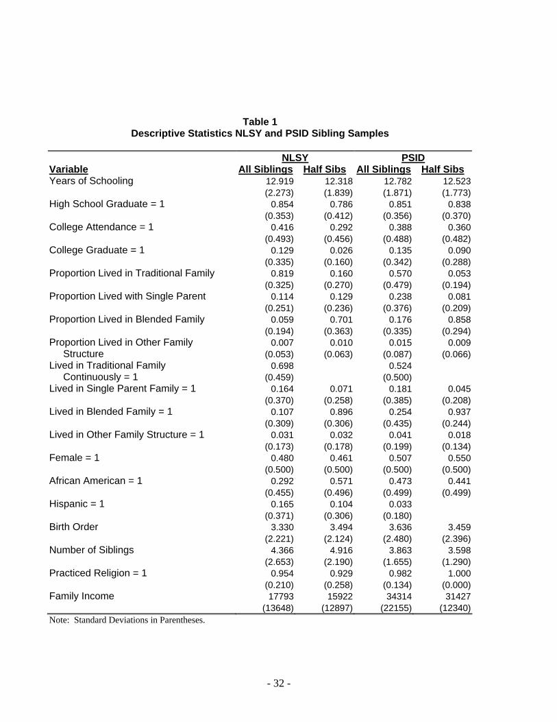
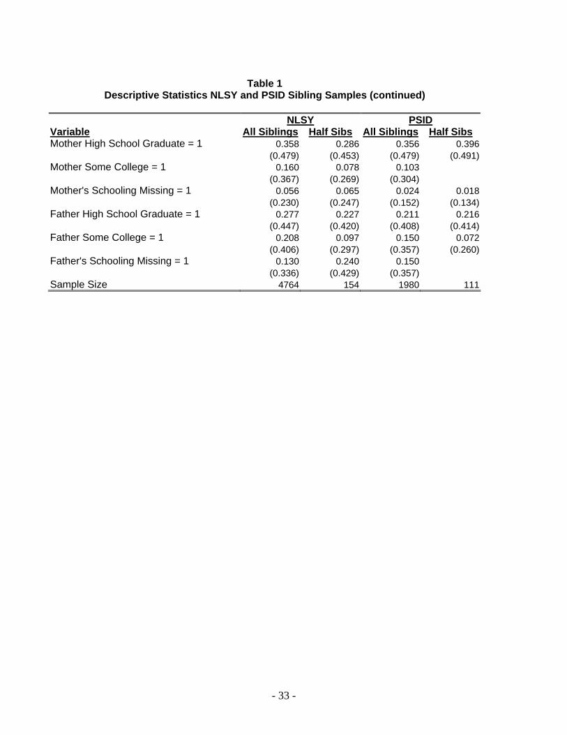
Table 1 reports the means and standard deviations of the variables used in the NLSY and PSID

siblings sample along with the stable blended family subsamples. Almost 30 percent of the siblings in

the NLSY and 48 percent of siblings in the PSID report ever living in a non-traditional family.13 Of

those children who have lived in a blended family in the PSID and NLSY, 75 percent have lived with a

stepfather whereas only 14 percent have lived with a stepmother. The remaining 11 percent are the

biological children of both parents in the blended family. Three percent of the siblings in the NLSY

(154 individuals) and eight percent in the PSID (111 individuals) lived in stable blended families.14

Within the stable blended family subsample, 39 percent of children have lived with a stepfather whereas

only 9 percent have lived with a stepmother. The remaining 52 percent are the biological children of

both parents in the stable blended family. Mean educational outcomes are lower in the stable blended

family subsamples than for all siblings.

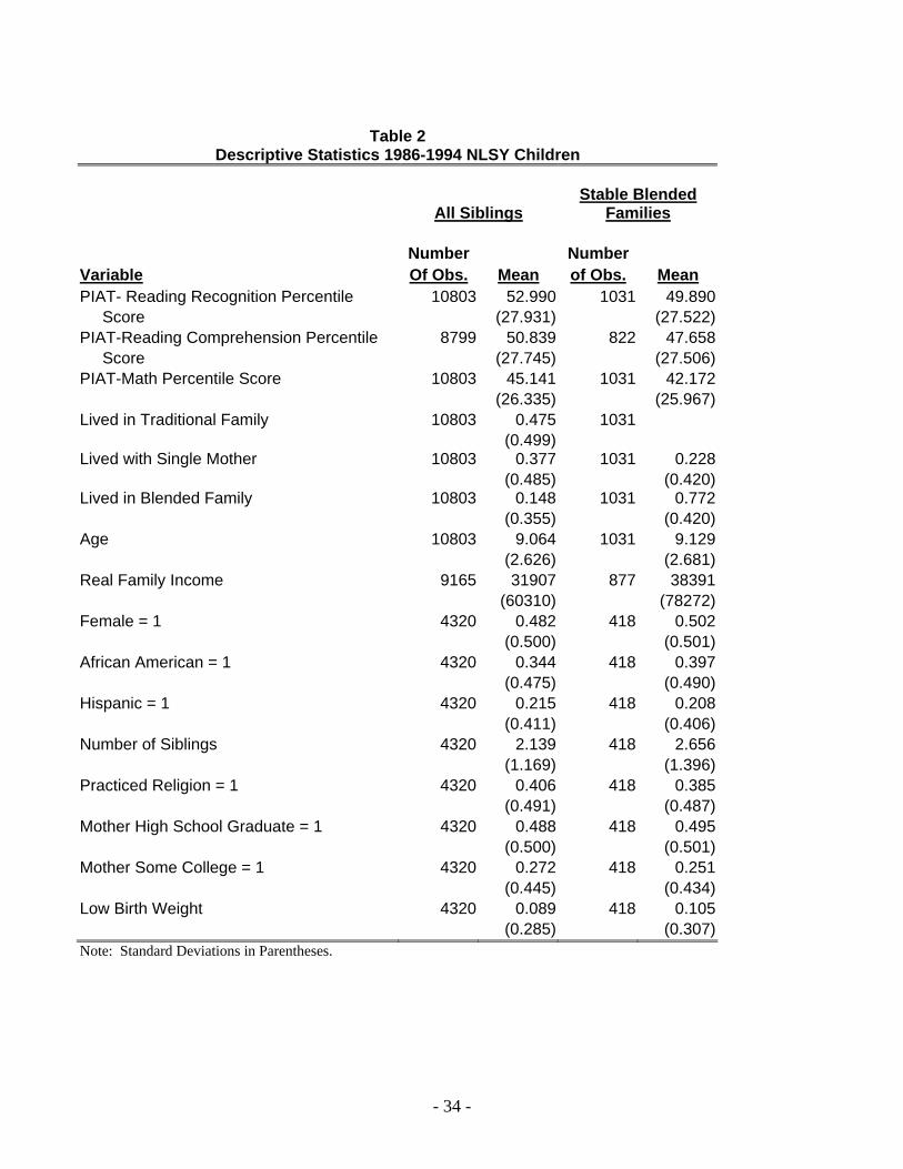
Table 2 reports the descriptive statistics for the NLSY-Child sample and our stable blended

family subsample. There are 4,320 siblings in the sample, of whom 418 individuals live in stable

blended families. Children in the NLSY-Child sample are repeatedly assessed, so we have over 10,000

child-year observations in this data set. Mean reading and math assessment scores are lower in stable

blended families than for all of the siblings in the NLSY-Child sample. By definition, children in

blended families in the NLSY-Child are the biological children of the mother and live with either their

biological father or a stepfather.

13 The percentage of siblings living in non-traditional families is greater in the PSID because of the oversampling of disadvantaged families. 14 Because our blended families are defined as families that remain together for the entire childhood of at least one child, these percentages are not an estimate of the percentage of children in the population who spend some portion of their childhood in a family that includes a husband, a wife, at least one stepchild, and at least one biological child of the couple.

- 17 -

We use these data to estimate the correlation between family structure and children’s educational

attainment making no attempt to control for the endogeneity of family structure. Instead, we focus on

the robustness of the correlation between children’s educational outcomes and family structure when we

use alternative definitions of family structure and introduce controls for family background variables.

We begin by estimating the correlation between family structure and educational outcomes using

two models, the entire sample of siblings, and our family-based measures of family structure. We are

motivated to take this approach by Biblarz and Raftery (1999) who show that the effect of family

structure is sensitive to which control variables are included. In addition to family structure, our first

model includes the exogenous variables of gender and race. We exclude variables that measure inputs

and behaviors chosen jointly with family structure, although several studies include such variables.15 In

order to examine the sensitivity of family structure estimates to the inclusion of other control variables,

we include variables such as sibship size (number of siblings), birth order, family income, religion, and

parental schooling in the second specification.

In our second approach, we compare outcomes for half-siblings within the same stable blended

family. We have defined our stable blended family samples in the NLSY and PSID to ensure that each

family includes at least one child reared by both biological parents until age 16.16 If growing up with

both biological parents has a substantial impact on children’s educational outcomes, we would expect to

find evidence of this in our stable blended family samples. That is, we would expect to find that

children reared by both biological parents have better outcomes than their half-siblings who spent time

in single-parent families and as stepchildren in stable blended families.

15 See for example, Biblarz and Raftery (1999), Manski et al. (1992), and Lang and Zagorsky (2001). 16 Stable blended families in the NLSY-Child are defined as at least one sibling living with both biological parents and a half-sibling in 1994.

- 18 -

EMPIRICAL RESULTS The Correlation Between Family Structure and Educational Outcomes

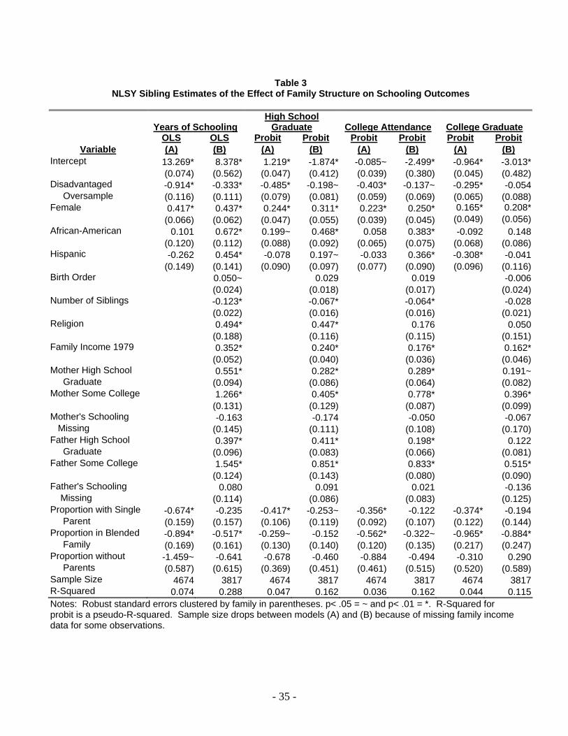
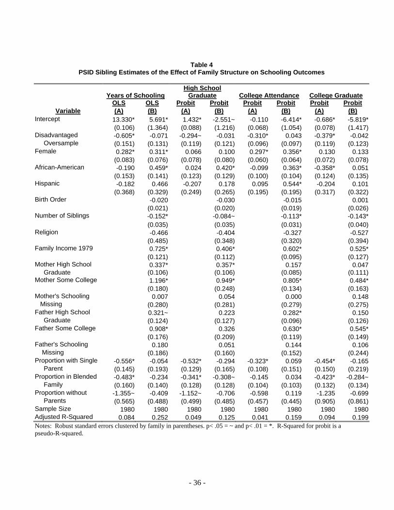
We begin by estimating two cross-section models of the effect of family structure on schooling

outcomes. Model (A) regresses schooling outcomes on variables for gender, race, an indicator for being

in the disadvantaged subsample, and family structure. Model (B) adds measures for number of siblings,

birth order, family income, religion, and parental schooling to Model (A). Estimates using the NLSY

are presented in Table 3, and those using the PSID are presented in Table 4. All regression estimates

throughout the paper report standard errors that are clustered by family and adjusted using the Huber-

White method to account for the correlation between observations from the same family. The models

use family-based measures of family structure; all models have measures for the proportion of childhood

spent in a single-parent family, blended family, or other family structure with proportion spent in a

traditional nuclear family being the omitted category. We can interpret the coefficient on proportion of

childhood in a given family structure as the effect on schooling of spending an additional fraction of

childhood in that family structure and correspondingly less in a traditional nuclear family.

Like previous research, our OLS and probit cross-section estimates of Models (A) in both data

sets show that proportion spent with a single-parent family or blended family have negative and

significant effects on schooling outcomes. As additional variables are included in Model (B), we

observe results similar to those in Biblarz and Raftery (1999). The estimated effect of growing up with

a single-parent attenuates and is not statistically significant in seven of the eight models estimated in

Tables 3 and 4. In estimates not reported here, we find that much of the attenuation in the effect of

single-parent families on educational outcomes results from the inclusion of family income in Model B.

The estimated effect of growing up in a blended family is less negative in model B than in model A, but

- 19 -

the coefficients remain negative and statistically significant in five of the eight models. Our results

suggest that the estimated effect of family structure is sensitive to the inclusion of other variables in the

regression.17 After controlling for additional variables, blended families are more negatively correlated

with lower educational attainment than single-parent families.

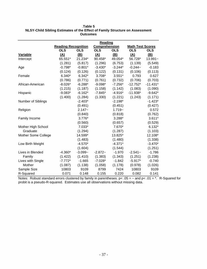
We now turn to the correlation of family structure with child assessment outcomes. Table 5

presents two sets of estimates for each of three child assessment outcomes (reading recognition, reading

comprehension, and math). In the first OLS specification, Model (A), the normalized percentile

assessment scores for each outcome is regressed on variables for age, gender, race, and family structure.

Model (B) adds number of siblings, religion, mother's schooling, family income, and an indicator for

low birth weight to Model (A). Family structure is measured as an indicator variable for each year an

individual is in the data set. The results for Model (A) indicate that living with a single parent or in a

blended family significantly decreases reading and math scores. The estimated effect of family structure

on assessment outcomes decreases substantially in Model (B) when additional variables are included in

the regression.18 More specifically, the results for Model B indicate that living with a single-parent or in

a blended family is always negative. But of the six family structure coefficients reported in Table 5

only one, the effect on reading recognition of living in a blended family, attains statistical significance.

17 We have experimented with alternative specifications in Tables 3 and 4 and found our results to be robust. In appendix tables B.1 and B.2 we use dummy variables for family structure instead of proportion living in a particular family structure. The estimates presented in Tables 3 and 4 fit the data better than those using family structure dummies but tell the same story. 18 In results available from the authors by request, we find similar estimated effects of family structure on the behavioral problems index.

- 20 -

Blended Families Estimates

We next consider educational outcomes in stable blended families. We begin with schooling

attainment. Because our stable blended-family sample is small in each data set, we combine the blended

family subsamples from the PSID and NLSY for this analysis. Appendix Tables B.3 through B.6

contain separate analyses for the PSID and NLSY blended family subsamples. We begin with simple

tests of differences in mean schooling. The top panel of Table 6 tests the null hypothesis of no

difference in mean schooling between siblings from stable blended families and siblings from traditional

nuclear families in the combined PSID-NLSY sample. For all four schooling outcomes we reject the

null hypothesis of no difference. Mean schooling outcomes in the stable blended-family sample are

substantially and significantly lower than those for children from traditional nuclear families.19

Next, we compare the mean educational outcomes for joint biological children from stable

blended families with outcomes for children from traditional nuclear families. In the middle panel of

Table 6 we see that in three of the four outcomes joint biological children from blended families have

significantly lower educational attainment.

Finally, we evaluate whether schooling outcomes within the stable blended-family sample differ

for the stepchildren and the joint biological children. These results are presented in the bottom panel of

Table 6. For three of the four schooling outcomes, children growing up with both biological parents in

stable blended families do better than the stepchildren.

For the fourth schooling outcome, graduation from college, stepchildren do better than the joint

biological children, but the sample size is very small: only 14 individuals in the blended family sample

19 These results do not change when non-stable blended family are included in the analysis.

- 21 -

are college graduates. Furthermore, the difference between the stepchildren and the joint biological

children in stable blended families is not statistically significant. Comparing the bottom panel of Table 6

with the top panel, we see that the differences in mean schooling outcomes within the blended family are

small relative to the difference between blended family schooling outcomes and those of children in

traditional nuclear families. Given the lack of statistical significance and the small sample size, we

could be committing a Type II error of accepting the null hypothesis when the null is false. To examine

this possibility, we estimated the power of the hypothesis tests in the bottom panel of Table 6 assuming

a five percent level of significance. All of the hypothesis tests in the bottom panel of Table 6 have

estimated power equal to one, suggesting a negligible chance of committing a Type II error.

In Table 7, we estimate two models of schooling using the stable blended-family sample.20

Model (A) is a parsimonious model where family structure is measured as proportion of childhood in a

non-intact family. We use this variable because it captures the differences between the step and joint

biological children in the blended families. Model (B) includes additional family background

characteristics. In both models, the proportion of childhood spent in a non-intact family has a negative

and statistically insignificant effect on educational attainment.21

Our results on the impact of family structure on educational attainment can be summarized as

follows: Using family-based measures of family structure, estimates of the effect of living with a single

parent differ significantly depending on which family background variables are included in the model.

Regardless of the specification employed, the effect of living in a blended family remains negative and

significant. In the stable blended families sample, the differences in educational outcomes between the

joint biological and stepchildren is small and both types of children from blended families do poorly

20 Only three of the four schooling outcomes are presented in Table 7 because only 14 individuals in the blended-family sample graduated from college. 21 This result also holds when the models are estimated separately for the PSID and NLSY. See Appendix Tables B.5 and B.6.

- 22 -

when compared with children from traditional nuclear families. The tests of mean differences indicate

that growing up in a stable blended family has a negative impact on schooling outcomes for both

stepchildren and joint biological children. In the stable blended family regressions, stepchildren do

somewhat worse than joint biological children, but the difference is small and not statistically

significant.22

We now turn to the effect of family structure on the three child assessment outcomes. Table 8

reports results of tests of mean differences in the assessment outcomes for children in the NLSY-Child

sample. The first panel in Table 8 shows statistically significant differences in mean outcomes between

the children in the stable blended family sample and children from traditional nuclear families in the

NLSY-Child sample. For all three outcomes, we reject the null hypothesis of no difference in mean

scores across the two groups. The second panel of Table 8 compares the mean outcomes for joint

biological children in stable blended families with children from traditional nuclear families. We again

see large differences: the children in traditional nuclear families have substantially better outcomes.

The bottom panel of Table 8 reports mean outcomes within the stable blended family sample, comparing

the stepchildren (“her children” ) with the joint biological children of both parents (“their children”).

We find that stepchildren have lower mean scores on both reading assessments and the math assessment.

When we test the null hypothesis that there is no mean difference in outcomes between “her children”

and “their children,” we again fail to reject the null hypothesis: we find no significant difference in mean

outcomes of the step children and the joint biological children in stable blended-families. We evaluated

the power at the five percent level of significance of the hypothesis tests in the bottom panel of Table 8.

22 Case, Lin, and McLanahan, (2002) find that stepchildren in stepmother families do substantially and significantly worse than biological children in these families. However, they also find no significant difference in educational outcomes between stepchildren and biological children in stepfather blended families. As discussed in section 2, the majority of children in our sample are from stepfather blended families.

- 23 -

The reading comprehension and math hypothesis tests have estimated power of one and 0.998

respectively, suggesting a negligible chance of committing a Type II error. The reading recognition test

has less power at 0.784.

Finally, in Table 9 we present regression estimates of the effect of family structure on children’s

assessments using the NLSY-Child stable blended-family sample. Results for Models (A) and (B) are

presented in the table for the three assessments. We find that living in a single-parent or a blended

family generally has a positive but insignificant effect on the PIAT assessments. Only one of the family

structure variables is statistically significant in Table 9: living with a single parent has a positive and

statistically significant effect on reading comprehension, even after controlling for family background

characteristics.

Tables 8 and 9 indicate that stable blended family child assessment outcomes differ from the full

NLSY-Child sample. Comparing the effect of family structure using the stable blended-family sample,

we find that the estimated coefficients on the family structure variables often change signs and generally

become statistically insignificant. Our results are based on 418 observations which should be sufficient

to generate statistically significant point estimates. Using the NLSY-Child data and mother-fixed effects

estimates for blended families, Gennetian (Forthcoming) finds essentially the same results.

Our estimates show that outcomes for both types of children in stable blended families--

stepchildren and their half-siblings who are the joint biological children of both parents are substantially

worse than for children reared in traditional nuclear families. Because these estimated correlations are

merely the result of regressing one endogenous variable on another, however, they do not provide a

basis for policy.

- 24 -

CONCLUSION

In this paper we have augmented the stock of stylized facts and descriptive regressions that summarize

the correlations between family structure and children’s educational outcomes. Our results pertain only

to educational outcomes and may not generalize to other outcomes such as health or teen pregnancy.

Our contribution to the stock of stylized facts concerns blended families. It is well-known that, on

average, children reared in traditional nuclear families have substantially better educational outcomes

than stepchildren from stable blended families. We find that children reared in traditional nuclear

families also have substantially better educational outcomes than the joint biological children from

stable blended families. Within stable blended families we find that the difference between the joint

biological children and the stepchildren is neither substantial nor statistically significant.

Controlling not only for family structure but also for variables such as mothers' education and

family income, descriptive regressions reveal a different pattern of family structure effects than the

stylized facts which control only for family structure. With additional controls, the effect of family

structure falls substantially and often loses statistical significance. In particular, the effect of living in a

single-parent family is no longer statistically significant after controlling for family income.

How can we understand these findings? Four explanations, separately or in combination, might

account for at least some of them. First, family structure may well be a proxy for other variables that

affect outcomes for children. If family structure is correlated with family resources (e.g., time and money)

devoted to children and if we fail to control for these variables, then family structure will pick up some of

their effects. Because descriptive regressions do not correspond to either structural or reduced form

- 25 -

relationships, there is no principled way to argue about which variables ought to be included and which

excluded from descriptive regressions.23

The second explanation is stress. Although the Brady Bunch was preternaturally happy, the

presence of stepchildren is often described as a source of stress. The sociologist Andrew Cherlin (1978)

characterized remarriage as an "incomplete institution," arguing that roles in such families lack clear

definition; for example, there is no consensus about when it is appropriate for a stepfather to discipline a

stepchild. Most discussions of blended families focus on outcomes for stepchildren. Few researchers

have discussed the joint biological children in blended families, although Gennetian (Forthcoming) is an

important exception. The stresses and strains of blended families -- the presence of stepchildren, not

necessarily their behavior -- might affect outcomes for the joint biological children as well as the

stepchildren. Stress might explain why children in blended families have worse educational outcomes

than children in other two-parent families.

Some have suggested that the number of family structure transitions experienced by stepchildren

and by children in single parent families explains the poor outcomes they experience. Although we do

not systematically examine the effects of the number of family structure transitions, our findings for

educational outcomes of biological children in stable blended families cannot be explained in this way.

The biological children in stable blended families grew up with both biological parents and experienced

no family structure transitions. Yet their educational outcomes are similar to those experienced by

23 The discussion of the effect of family resources on outcomes for children provides an example. The papers in Duncan and Brooks-Gunn (1996) generally argue that increases in family resources have positive effects on child outcomes; Mayer (1997) argues that most of the observed correlation between family resources and child outcomes reflects unobserved heterogeneity; Blau (1999) provides a balanced summary of the discussion. The underlying difficulty is that the discussion of family resource effects, like the discussion of family structure effects, requires a well-specified counterfactual (e.g., an increase in cash welfare benefits; winning the lottery), but discussions of counterfactuals are conspicuously absent.

- 26 -

stepchildren and by children in single parent families, and much worse than those experienced by

children in traditional nuclear families.24

The third explanation hinges on the allocation of time and other resources within blended

families. If mothers allocate resources among children within blended families, and if all of the children

are hers, as they usually are, then she may use her ability to allocate resources to "compensate" for any

negative effects of family structure on stepchildren. This explanation highlights the fact that observed

educational outcomes are not "pure" family structure effects, whatever that might mean, but also reflect

the effects of any compensating or reinforcing family allocation decisions.

The fourth explanation is heterogeneity. Observed heterogeneity draws our attention to which of

the observed variables investigators choose to control for. The descriptive regressions show that the

correlations between family structure and outcomes for children fall substantially and often lack

statistical significance when we control for variables such as mothers' education and family income.

Unobserved heterogeneity draws our attention to differences in unobserved behaviors that may influence

outcomes for children but also to differences in preferences and ability that influence the choice of

family structure, education, and childbearing. Parents in blended families and single-parent families that

result from divorce or nonmarital fertility may differ from parents in traditional nuclear families in

unobserved as well as observed characteristics. Even if family structure has no "direct" or "causal"

effect on outcomes for children, unobserved heterogeneity and selection could account for the

association between outcomes for children and family structure summarized in the stylized facts and

descriptive regressions.

24 The fact that children of widows have educational outcomes similar to those of children in traditional nuclear families also casts doubt on the importance of the number of family structure transitions.

- 27 -

Our analysis also demonstrates, if another demonstration were needed, that what we see depends

on the lens we look through -- the classification scheme we bring to the analysis. Classification schemes

illuminate some relationships and obscure others. Furthermore, as Bowker and Star (1999) emphasize,

classification schemes themselves often become visible only when alternatives appear. Using a family-

based rather than a child-based classification of family structure, we see the children in blended families

-- the step children and the joint biological children -- in a new light.

Although we have augmented the set of stylized facts regarding family structure, we conclude by

emphasizing that stylized facts and descriptive regressions cannot support either scientific conclusions

or policy analysis. Counterfactuals are required. In economics most questions have default

counterfactuals that are not spelled out explicitly because they are generally understood. Questions

about the effect of family structure lack default counterfactuals. Interpreted literally, the question

"What is the effect of family structure on outcomes for children?" is ill-posed because it asks about the

effect of one endogenous variable on another. We argue for clarifying the family structure question by

specifying an explicit counterfactual.

Any counterfactual will clarify the question, but policy analysis requires policy-relevant

counterfactuals: the death of a parent provides a counterfactual, but not one that is useful for policy

analysis. In contrast, the effect of a change in the income tax that reduces the marriage penalty or a

change in state divorce laws on outcomes for children provide policy relevant counterfactuals. Gruber

(Forthcoming) investigates the effect of unilateral divorce on outcomes for children, using state-to-state

differences in the timing of the "divorce revolution" -- the transition from fault based divorce, to divorce

by mutual consent, to unilateral divorce. Gruber finds that unilateral divorce has a negative and

significant effect on children's educational attainment. Although Gruber does not use the language of

counterfactuals, he reviews the family structure literature, which generally claims that divorce has

- 28 -

adverse effects on outcomes for children, and criticizes it for failing to recognize and deal with the

endogeneity of family structure.

Our results imply cautions for policy. Neither stylized facts nor descriptive regressions provide

defensible estimates of effects of family structure. Designers of policy interventions need to know more

about the determinants of outcomes for children than they can learn from stylized facts and descriptive

regressions. Policies intended to improve outcomes for children often focus on family structure, which is

easy to observe and, some believe, relatively easy to influence through tax and welfare policy, couple

counseling, or legal rules governing marriage, divorce, and child support. If the stylized facts about the

relationship between outcomes for children and family structure reflect the influences of variables other

than family structure, then policies that affect family structure may have little or no effect on outcomes

for children. Our blended family results and our descriptive regressions results call into question the

causal interpretation of the stylized facts about the relationship between family structure and outcomes

for children.

- 29 -

REFERENCES Biblarz, T. J. and G. Gottainer. 2000. “Family Structure and Children’s Success: A Comparison of

Widowed and Divorced Single-Mother Families.” Journal of Marriage and Family 62:533-48. Biblarz, T. J. and A. E. Raftery. 1999. “Family Structure, Educational Attainment, and Socioeconomic

Success: Rethinking the ‘Pathology of Matriarchy.’” American Journal of Sociology 105:321-65. Björklund, A. and M. Sundström. 2002. “Parental Separation and Children’s Educational Attainment:

A Siblings Approach.” Discussion Paper No. 643, IZA, Bonn. Blau, D. M. 1999. "The Effect of Income on Child Development." Review of Economics and Statistics

81:261-76. Boggess, S. 1998.“Family Structure, Economic Status, and Educational Attainment.” The Journal of

Population Economics 11:205-22. Bowker, G. C. and S.L. Star. 1999. Sorting Things Out: Classification and its Consequences.

Cambridge: MIT Press. Case, A., I. Lin, and S. McLanahan. 2001. “Educational Attainment of Siblings in Stepfamilies.”

Evolution and Human Behavior 22:269-89. Cherlin, A. J. 1978. "Remarriage as an Incomplete Institution." American Journal of Sociology 84:634-

50. Cherlin, A. J. and F.F. Furstenberg, Jr. 1994. "Stepfamilies in the United States: A Reconsideration."

Annual Review of Sociology 20:359-81. Cherlin, A. J., F. F. Furstenberg, Jr., P. L. Chase-Lansdale, K. E. Kiernan, P. K. Robins,

D. R. Morrison, and J. O. Teitler. 1991. “Longitudinal Studies of Effects of Divorce on Children in Great Britain and the United States.” Science 252:1386-89.

Corak, M. 2001.“Death and Divorce: The Long-Term Consequences of Parental Loss on Adolescents.”

Journal of Labor Economics 19:682-715. Current Population Reports P23-181. 1992. “Households, Families, and Children: A 30-Year

Perspective.” Washington, D.C: U.S. Government Printing Office. Daly, M. and M. I. Wilson. 1999. The Truth about Cinderella: A Darwinian View of Parental Love.

New Haven: Yale University Press. -------. 2000. "The Evolutionary Psychology of Marriage and Divorce," Pp. 91-110 in Ties that Bind:

Perspectives on Marriage and Cohabitation edited by L. Waite, C. Bachrach, M. Hindin, E. Thomson, and A. Thornton. New York: Aldine de Gruyter.

- 30 -

Department of Health and Human Services. 1996. Trends in the Well-Being of America’s Children and Youth. Washington, D.C: U.S. Government Printing Office.

Duncan, G. J. and J. Brooks-Gunn, eds. 1996. Consequences of Growing Up Poor. New York: Russell

Sage Foundation. Eckstein, Z. and K. I. Wolpin. 1999. “Why Youths Drop Out of High School: The Impact of

Preferences, Opportunities, and Abilities.” Econometrica 67:1295-339. Ermisch, J. F. and M. Francesconi. 2001. “Family Structure and Children’s Achievements.” Journal of

Population Economics 14:249-70. Evenhouse, E. and S. Reilly. 2004.“A Sibling Study of Stepchild Well-Being.” Journal of Human

Resources 39:248-76. Gennetian, L. Forthcoming. “One or Two Parents? Half or Step Siblings? The Effect of Family

Composition on Young Children’s Achievement.” Journal of Population Economics. Gruber, J. Forthcoming. “Is Making Divorce Easier Bad for Children? The Long Run Implications of

Unilateral Divorce.” Journal of Labor Economics. Haveman, R. and B. Wolfe. 1994. Succeeding Generations: On the Effects of Investments in Children.

New York: Russell Sage Foundation. -------- 1995. “The Determinants of Children’s Attainments: A Review of Methods and Findings.”

Journal of Economic Literature 33:1829-78. Lang, K. and J. L. Zagorsky. 2001. “Does Growing Up With a Parent Absent Really Hurt?" Journal of

Human Resources 36:253-73. McLanahan, S. and G. Sandefur. 1994. Growing Up with a Single Parent: What Hurts, What Helps.

Cambridge: Harvard University Press. Manski, C., G. D. Sandefur, S. McLanahan, and D. Powers. 1992. “Alternative Estimates of the Effect

of Family Structure During Adolescence on High School Graduation.” Journal of the American Statistical Association 87:25-37.

Mayer, S. E. 1997. What Money Can't Buy: Family Income and Children's Life Chances. Cambridge:

Harvard University Press. NLSY79 User’s Guide Handbook. 1997. Columbus, Ohio: Center for Human Resource Research, The

Ohio State University. Painter, G. and D. I. Levine. 2000. “Family Structure and Youths’ Outcomes: Which Correlations Are

Causal?” Journal of Human Resources 35:524-49.

- 31 -

Thomson, E., T. L. Hanson, and S. S. McLanahan. 1994. “Family Structure and Child Well-Being: Economic Resources vs. Parental Behaviors.” Social Forces 73:221-42.

Weiss, Y. and R. J. Willis. 1985. "Children as Collective Goods in Divorce Settlements." Journal of

Labor Economics 3:268-92. Weiss, Y. and R. J. Willis. 1993. "Transfers among Divorced Couples: Evidence and Interpretation."

Journal of Labor Economics 11:629-79. Wojtkiewicz, R. A. 1993. “Simplicity and Complexity in the Effects of Parental Structure on High

School Graduation.” Demography 30:701-17. Wolfe, B., R. Haveman, D. Ginther, and C. B. An. 1996. “The ‘Window Problem’ in Studies of

Children’s Attainments: A Methodological Exploration.” Journal of the American Statistical Association 91:970-82.

Wu, L. L. and B. C. Martinson. 1993. "Family Structure and the Risk of a Premarital Birth." American

Sociological Review 58:210-32.

- 32 -

Table 1 Descriptive Statistics NLSY and PSID Sibling Samples

NLSY PSID

Variable All Siblings Half Sibs All Siblings Half Sibs Years of Schooling 12.919 12.318 12.782 12.523

(2.273) (1.839) (1.871) (1.773)High School Graduate = 1 0.854 0.786 0.851 0.838

(0.353) (0.412) (0.356) (0.370)College Attendance = 1 0.416 0.292 0.388 0.360

(0.493) (0.456) (0.488) (0.482)College Graduate = 1 0.129 0.026 0.135 0.090

(0.335) (0.160) (0.342) (0.288)Proportion Lived in Traditional Family 0.819 0.160 0.570 0.053 (0.325) (0.270) (0.479) (0.194)Proportion Lived with Single Parent 0.114 0.129 0.238 0.081

(0.251) (0.236) (0.376) (0.209)Proportion Lived in Blended Family 0.059 0.701 0.176 0.858

(0.194) (0.363) (0.335) (0.294)Proportion Lived in Other Family 0.007 0.010 0.015 0.009 Structure (0.053) (0.063) (0.087) (0.066)Lived in Traditional Family 0.698 0.524 Continuously = 1 (0.459) (0.500) Lived in Single Parent Family = 1 0.164 0.071 0.181 0.045

(0.370) (0.258) (0.385) (0.208)Lived in Blended Family = 1 0.107 0.896 0.254 0.937

(0.309) (0.306) (0.435) (0.244)Lived in Other Family Structure = 1 0.031 0.032 0.041 0.018

(0.173) (0.178) (0.199) (0.134)Female = 1 0.480 0.461 0.507 0.550

(0.500) (0.500) (0.500) (0.500)African American = 1 0.292 0.571 0.473 0.441

(0.455) (0.496) (0.499) (0.499)Hispanic = 1 0.165 0.104 0.033

(0.371) (0.306) (0.180) Birth Order 3.330 3.494 3.636 3.459

(2.221) (2.124) (2.480) (2.396)Number of Siblings 4.366 4.916 3.863 3.598

(2.653) (2.190) (1.655) (1.290)Practiced Religion = 1 0.954 0.929 0.982 1.000

(0.210) (0.258) (0.134) (0.000)Family Income 17793 15922 34314 31427

(13648) (12897) (22155) (12340)Note: Standard Deviations in Parentheses.

- 33 -

Table 1

Descriptive Statistics NLSY and PSID Sibling Samples (continued)

NLSY PSID Variable All Siblings Half Sibs All Siblings Half Sibs Mother High School Graduate = 1 0.358 0.286 0.356 0.396

(0.479) (0.453) (0.479) (0.491)Mother Some College = 1 0.160 0.078 0.103

(0.367) (0.269) (0.304) Mother's Schooling Missing = 1 0.056 0.065 0.024 0.018

(0.230) (0.247) (0.152) (0.134)Father High School Graduate = 1 0.277 0.227 0.211 0.216

(0.447) (0.420) (0.408) (0.414)Father Some College = 1 0.208 0.097 0.150 0.072

(0.406) (0.297) (0.357) (0.260)Father's Schooling Missing = 1 0.130 0.240 0.150

(0.336) (0.429) (0.357) Sample Size 4764 154 1980 111

- 34 -

Table 2

Descriptive Statistics 1986-1994 NLSY Children

All Siblings

Stable Blended

Families Number Number Variable Of Obs. Mean of Obs. Mean PIAT- Reading Recognition Percentile 10803 52.990 1031 49.890 Score (27.931) (27.522) PIAT-Reading Comprehension Percentile 8799 50.839 822 47.658 Score (27.745) (27.506) PIAT-Math Percentile Score 10803 45.141 1031 42.172

(26.335) (25.967) Lived in Traditional Family 10803 0.475 1031

(0.499) Lived with Single Mother 10803 0.377 1031 0.228

(0.485) (0.420) Lived in Blended Family 10803 0.148 1031 0.772

(0.355) (0.420) Age 10803 9.064 1031 9.129

(2.626) (2.681) Real Family Income 9165 31907 877 38391 (60310) (78272) Female = 1 4320 0.482 418 0.502 (0.500) (0.501) African American = 1 4320 0.344 418 0.397 (0.475) (0.490) Hispanic = 1 4320 0.215 418 0.208 (0.411) (0.406) Number of Siblings 4320 2.139 418 2.656 (1.169) (1.396) Practiced Religion = 1 4320 0.406 418 0.385 (0.491) (0.487) Mother High School Graduate = 1 4320 0.488 418 0.495

(0.500) (0.501) Mother Some College = 1 4320 0.272 418 0.251

(0.445) (0.434) Low Birth Weight 4320 0.089 418 0.105

(0.285) (0.307) Note: Standard Deviations in Parentheses.

- 35 -

Table 3

NLSY Sibling Estimates of the Effect of Family Structure on Schooling Outcomes

Years of Schooling

High School Graduate

College Attendance

College Graduate

OLS OLS Probit Probit Probit Probit Probit Probit Variable (A) (B) (A) (B) (A) (B) (A) (B)

Intercept 13.269* 8.378* 1.219* -1.874* -0.085~ -2.499* -0.964* -3.013* (0.074) (0.562) (0.047) (0.412) (0.039) (0.380) (0.045) (0.482)

Disadvantaged -0.914* -0.333* -0.485* -0.198~ -0.403* -0.137~ -0.295* -0.054 Oversample (0.116) (0.111) (0.079) (0.081) (0.059) (0.069) (0.065) (0.088)Female 0.417* 0.437* 0.244* 0.311* 0.223* 0.250* 0.165* 0.208*

(0.066) (0.062) (0.047) (0.055) (0.039) (0.045) (0.049) (0.056)African-American 0.101 0.672* 0.199~ 0.468* 0.058 0.383* -0.092 0.148

(0.120) (0.112) (0.088) (0.092) (0.065) (0.075) (0.068) (0.086)Hispanic -0.262 0.454* -0.078 0.197~ -0.033 0.366* -0.308* -0.041

(0.149) (0.141) (0.090) (0.097) (0.077) (0.090) (0.096) (0.116)Birth Order 0.050~ 0.029 0.019 -0.006

(0.024) (0.018) (0.017) (0.024)Number of Siblings -0.123* -0.067* -0.064* -0.028

(0.022) (0.016) (0.016) (0.021)Religion 0.494* 0.447* 0.176 0.050

(0.188) (0.116) (0.115) (0.151)Family Income 1979 0.352* 0.240* 0.176* 0.162*

(0.052) (0.040) (0.036) (0.046)Mother High School 0.551* 0.282* 0.289* 0.191~ Graduate (0.094) (0.086) (0.064) (0.082)Mother Some College 1.266* 0.405* 0.778* 0.396*

(0.131) (0.129) (0.087) (0.099)Mother's Schooling -0.163 -0.174 -0.050 -0.067 Missing (0.145) (0.111) (0.108) (0.170)Father High School 0.397* 0.411* 0.198* 0.122 Graduate (0.096) (0.083) (0.066) (0.081)Father Some College 1.545* 0.851* 0.833* 0.515* (0.124) (0.143) (0.080) (0.090)Father's Schooling 0.080 0.091 0.021 -0.136 Missing (0.114) (0.086) (0.083) (0.125)Proportion with Single -0.674* -0.235 -0.417* -0.253~ -0.356* -0.122 -0.374* -0.194 Parent (0.159) (0.157) (0.106) (0.119) (0.092) (0.107) (0.122) (0.144)Proportion in Blended -0.894* -0.517* -0.259~ -0.152 -0.562* -0.322~ -0.965* -0.884* Family (0.169) (0.161) (0.130) (0.140) (0.120) (0.135) (0.217) (0.247)Proportion without -1.459~ -0.641 -0.678 -0.460 -0.884 -0.494 -0.310 0.290 Parents (0.587) (0.615) (0.369) (0.451) (0.461) (0.515) (0.520) (0.589)Sample Size 4674 3817 4674 3817 4674 3817 4674 3817R-Squared 0.074 0.288 0.047 0.162 0.036 0.162 0.044 0.115Notes: Robust standard errors clustered by family in parentheses. p< .05 = ~ and p< .01 = *. R-Squared for probit is a pseudo-R-squared. Sample size drops between models (A) and (B) because of missing family income data for some observations.

- 36 -

Table 4 PSID Sibling Estimates of the Effect of Family Structure on Schooling Outcomes

Years of Schooling High School

Graduate

College Attendance

College Graduate OLS OLS Probit Probit Probit Probit Probit Probit

Variable (A) (B) (A) (B) (A) (B) (A) (B) Intercept 13.330* 5.691* 1.432* -2.551~ -0.110 -6.414* -0.686* -5.819*

(0.106) (1.364) (0.088) (1.216) (0.068) (1.054) (0.078) (1.417)Disadvantaged -0.605* -0.071 -0.294~ -0.031 -0.310* 0.043 -0.379* -0.042 Oversample (0.151) (0.131) (0.119) (0.121) (0.096) (0.097) (0.119) (0.123)Female 0.282* 0.311* 0.066 0.100 0.297* 0.356* 0.130 0.133

(0.083) (0.076) (0.078) (0.080) (0.060) (0.064) (0.072) (0.078)African-American -0.190 0.459* 0.024 0.420* -0.099 0.363* -0.358* 0.051

(0.153) (0.141) (0.123) (0.129) (0.100) (0.104) (0.124) (0.135)Hispanic -0.182 0.466 -0.207 0.178 0.095 0.544* -0.204 0.101

(0.368) (0.329) (0.249) (0.265) (0.195) (0.195) (0.317) (0.322)Birth Order -0.020 -0.030 -0.015 0.001

(0.021) (0.020) (0.019) (0.026)Number of Siblings -0.152* -0.084~ -0.113* -0.143*

(0.035) (0.035) (0.031) (0.040)Religion -0.466 -0.404 -0.327 -0.527

(0.485) (0.348) (0.320) (0.394)Family Income 1979 0.725* 0.406* 0.602* 0.525*

(0.121) (0.112) (0.095) (0.127)Mother High School 0.337* 0.357* 0.157 0.047 Graduate (0.106) (0.106) (0.085) (0.111)Mother Some College 1.196* 0.949* 0.805* 0.484*

(0.180) (0.248) (0.134) (0.163)Mother's Schooling 0.007 0.054 0.000 0.148 Missing (0.280) (0.281) (0.279) (0.275)Father High School 0.321~ 0.223 0.282* 0.150 Graduate (0.124) (0.127) (0.096) (0.126)Father Some College 0.908* 0.326 0.630* 0.545* (0.176) (0.209) (0.119) (0.149)Father's Schooling 0.180 0.051 0.144 0.106 Missing (0.186) (0.160) (0.152) (0.244)Proportion with Single -0.556* -0.054 -0.532* -0.294 -0.323* 0.059 -0.454* -0.165 Parent (0.145) (0.193) (0.129) (0.165) (0.108) (0.151) (0.150) (0.219)Proportion in Blended -0.483* -0.234 -0.341* -0.308~ -0.145 0.034 -0.423* -0.284~ Family (0.160) (0.140) (0.128) (0.128) (0.104) (0.103) (0.132) (0.134)Proportion without -1.355~ -0.409 -1.152~ -0.706 -0.598 0.119 -1.235 -0.699 Parents (0.565) (0.488) (0.499) (0.485) (0.457) (0.445) (0.905) (0.861)Sample Size 1980 1980 1980 1980 1980 1980 1980 1980Adjusted R-Squared 0.084 0.252 0.049 0.125 0.041 0.159 0.094 0.199Notes: Robust standard errors clustered by family in parentheses. p< .05 = ~ and p< .01 = *. R-Squared for probit is a pseudo-R-squared.

- 37 -

.Table 5 NLSY-Child Sibling Estimates of the Effect of Family Structure on Assessment

Outcomes

Reading Recognition

Reading Comprehension

Math Test Scores

OLS OLS OLS OLS OLS OLS Variable (A) (B) (A) (B) (A) (B) Intercept 65.551* 21.234* 90.458* 49.054* 56.728* 13.991~

(1.281) (5.817) (1.296) (6.753) (1.139) (5.549) Age -0.798* -0.801* -3.430* -3.244* -0.244~ -0.183

(0.124) (0.126) (0.122) (0.131) (0.106) (0.113) Female 6.340* 6.342* 3.708* 3.551* 0.793 0.627

(0.786) (0.771) (0.761) (0.732) (0.706) (0.703) African-American -8.026* -6.288* -9.098* -7.256* -12.752* -11.431*

(1.215) (1.187) (1.158) (1.142) (1.083) (1.090) Hispanic -9.083* -6.162* -7.845* -4.916* -11.938* -9.642*

(1.400) (1.284) (1.330) (1.221) (1.243) (1.171) Number of Siblings -2.403* -2.198* -1.423*

(0.491) (0.451) (0.427) Religion 2.147~ 1.719~ 0.572

(0.840) (0.818) (0.762) Family Income 3.776* 3.288* 3.611*

(0.560) (0.657) (0.529) Mother High School 7.033* 7.670* 6.132* Graduate (1.294) (1.287) (1.103) Mother Some College 14.599* 13.825* 12.108*

(1.483) (1.480) (1.338) Low Birth Weight -4.570* -4.371* -3.470*

(1.604) (1.544) (1.251) Lives in Blended -4.360* -3.099~ -2.872~ -1.970 -2.541~ -1.786 Family (1.422) (1.410) (1.383) (1.343) (1.251) (1.238) Lives with Single -7.772* -1.665 -7.028* -1.842 -5.917* -0.740 Mother (1.087) (1.138) (1.058) (1.178) (0.978) (1.026) Sample Size 10803 9109 8799 7424 10803 9109 R-Squared 0.071 0.148 0.155 0.220 0.082 0.141 Notes: Robust standard errors clustered by family in parentheses. p< .05 = ~ and p< .01 = *. R-Squared for probit is a pseudo-R-squared. Estimates use all observations without missing data.

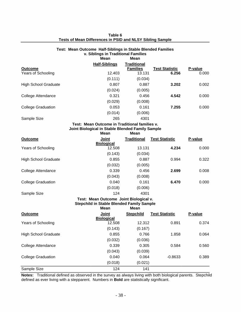
- 38 -

Table 6

Tests of Mean Differences in PSID and NLSY Sibling Sample

Test: Mean Outcome Half-Siblings in Stable Blended Families v. Siblings in Traditional Families

Mean Mean Outcome

Half-Siblings Traditional Families

Test Statistic

P-value

Years of Schooling 12.403 13.131 6.256 0.000 (0.111) (0.034) High School Graduate 0.807 0.887 3.202 0.002 (0.024) (0.005) College Attendance 0.321 0.456 4.542 0.000 (0.029) (0.008) College Graduation 0.053 0.161 7.255 0.000 (0.014) (0.006) Sample Size 265 4301

Test: Mean Outcome in Traditional families v. Joint Biological in Stable Blended Family Sample

Mean Mean Outcome Joint

Biological Traditional Test Statistic P-value

Years of Schooling 12.508 13.131 4.234 0.000 (0.143) (0.034) High School Graduate 0.855 0.887 0.994 0.322 (0.032) (0.005) College Attendance 0.339 0.456 2.699 0.008 (0.043) (0.008) College Graduation 0.040 0.161 6.470 0.000 (0.018) (0.006) Sample Size 124 4301

Test: Mean Outcome Joint Biological v. Stepchild in Stable Blended Family Sample

Mean Mean Outcome Joint

Biological Stepchild Test Statistic P-value

Years of Schooling 12.508 12.312 0.891 0.374 (0.143) (0.167) High School Graduate 0.855 0.766 1.858 0.064 (0.032) (0.036) College Attendance 0.339 0.305 0.584 0.560 (0.043) (0.039) College Graduation 0.040 0.064 -0.8633 0.389 (0.018) (0.021) Sample Size 124 141 Notes: Traditional defined as observed in the survey as always living with both biological parents. Stepchild defined as ever living with a stepparent. Numbers in Bold are statistically significant.

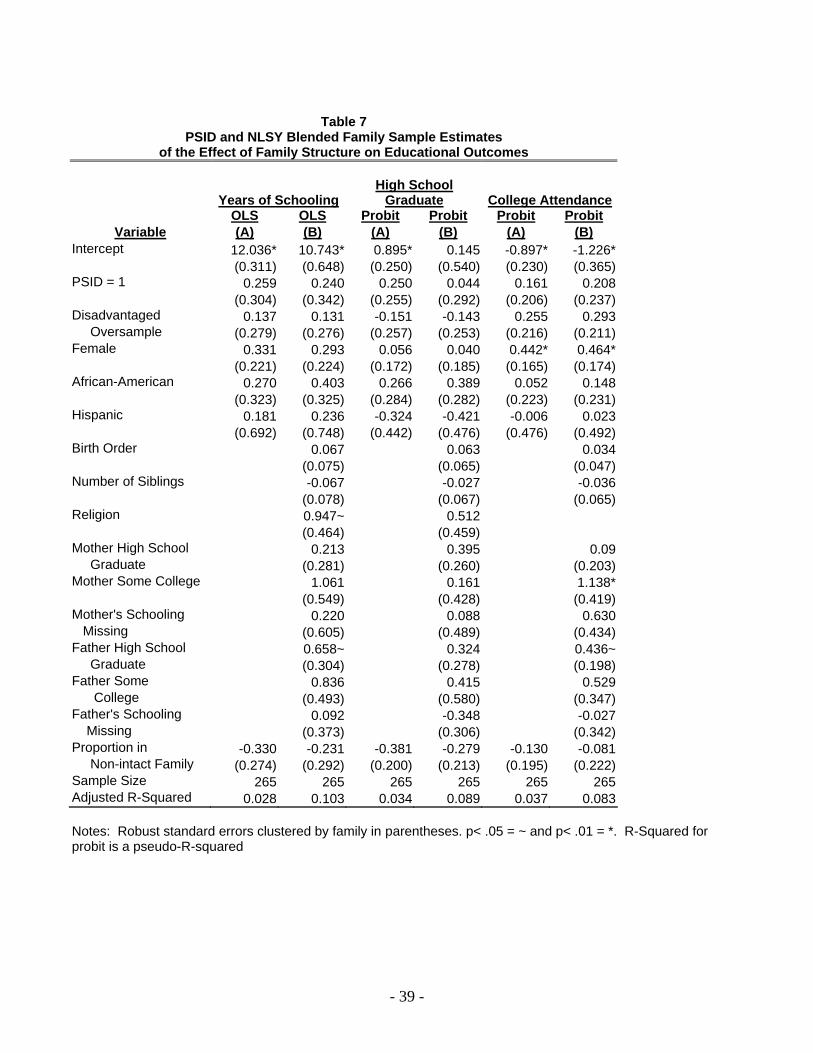
- 39 -

Table 7

PSID and NLSY Blended Family Sample Estimates of the Effect of Family Structure on Educational Outcomes

Years of Schooling

High School

Graduate

College Attendance OLS OLS Probit Probit Probit Probit

Variable (A) (B) (A) (B) (A) (B) Intercept 12.036* 10.743* 0.895* 0.145 -0.897* -1.226*

(0.311) (0.648) (0.250) (0.540) (0.230) (0.365) PSID = 1 0.259 0.240 0.250 0.044 0.161 0.208

(0.304) (0.342) (0.255) (0.292) (0.206) (0.237) Disadvantaged 0.137 0.131 -0.151 -0.143 0.255 0.293 Oversample (0.279) (0.276) (0.257) (0.253) (0.216) (0.211) Female 0.331 0.293 0.056 0.040 0.442* 0.464*

(0.221) (0.224) (0.172) (0.185) (0.165) (0.174) African-American 0.270 0.403 0.266 0.389 0.052 0.148

(0.323) (0.325) (0.284) (0.282) (0.223) (0.231) Hispanic 0.181 0.236 -0.324 -0.421 -0.006 0.023

(0.692) (0.748) (0.442) (0.476) (0.476) (0.492) Birth Order 0.067 0.063 0.034

(0.075) (0.065) (0.047) Number of Siblings -0.067 -0.027 -0.036

(0.078) (0.067) (0.065) Religion 0.947~ 0.512

(0.464) (0.459) Mother High School 0.213 0.395 0.09 Graduate (0.281) (0.260) (0.203) Mother Some College 1.061 0.161 1.138*

(0.549) (0.428) (0.419) Mother's Schooling 0.220 0.088 0.630 Missing (0.605) (0.489) (0.434) Father High School 0.658~ 0.324 0.436~ Graduate (0.304) (0.278) (0.198) Father Some 0.836 0.415 0.529 College (0.493) (0.580) (0.347) Father's Schooling 0.092 -0.348 -0.027 Missing (0.373) (0.306) (0.342) Proportion in -0.330 -0.231 -0.381 -0.279 -0.130 -0.081 Non-intact Family (0.274) (0.292) (0.200) (0.213) (0.195) (0.222) Sample Size 265 265 265 265 265 265 Adjusted R-Squared 0.028 0.103 0.034 0.089 0.037 0.083 Notes: Robust standard errors clustered by family in parentheses. p< .05 = ~ and p< .01 = *. R-Squared for probit is a pseudo-R-squared

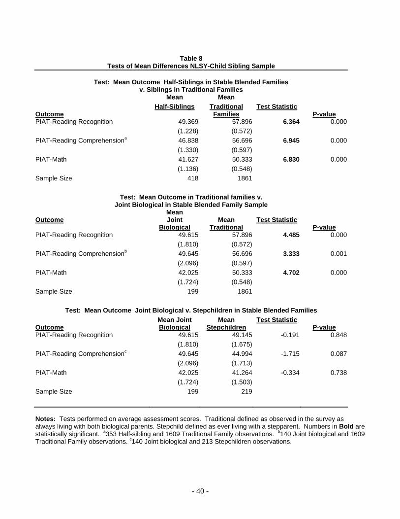
- 40 -

Table 8

Tests of Mean Differences NLSY-Child Sibling Sample

Test: Mean Outcome Half-Siblings in Stable Blended Families v. Siblings in Traditional Families

Mean Mean Outcome

Half-Siblings Traditional Families

Test Statistic P-value

PIAT-Reading Recognition 49.369 57.896 6.364 0.000 (1.228) (0.572) PIAT-Reading Comprehensiona 46.838 56.696 6.945 0.000 (1.330) (0.597) PIAT-Math 41.627 50.333 6.830 0.000 (1.136) (0.548) Sample Size 418 1861

Test: Mean Outcome in Traditional families v.

Joint Biological in Stable Blended Family Sample Outcome

Mean Joint

Biological

Mean

Traditional

Test Statistic

P-value PIAT-Reading Recognition 49.615 57.896 4.485 0.000 (1.810) (0.572) PIAT-Reading Comprehensionb 49.645 56.696 3.333 0.001 (2.096) (0.597) PIAT-Math 42.025 50.333 4.702 0.000 (1.724) (0.548) Sample Size 199 1861

Test: Mean Outcome Joint Biological v. Stepchildren in Stable Blended Families Outcome

Mean Joint Biological

Mean Stepchildren

Test Statistic P-value

PIAT-Reading Recognition 49.615 49.145 -0.191 0.848 (1.810) (1.675) PIAT-Reading Comprehensionc 49.645 44.994 -1.715 0.087 (2.096) (1.713) PIAT-Math 42.025 41.264 -0.334 0.738 (1.724) (1.503) Sample Size 199 219 Notes: Tests performed on average assessment scores. Traditional defined as observed in the survey as always living with both biological parents. Stepchild defined as ever living with a stepparent. Numbers in Bold are statistically significant. a353 Half-sibling and 1609 Traditional Family observations. b140 Joint biological and 1609 Traditional Family observations. c140 Joint biological and 213 Stepchildren observations.

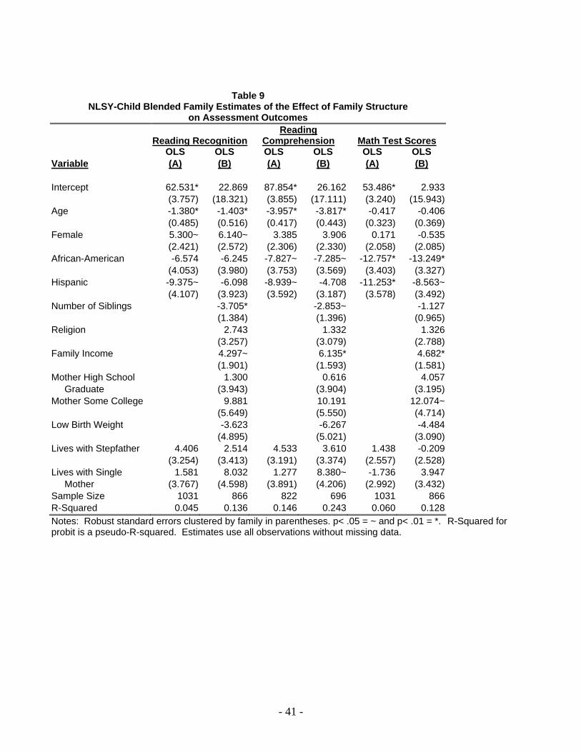
- 41 -

Table 9 NLSY-Child Blended Family Estimates of the Effect of Family Structure

on Assessment Outcomes Reading Recognition

Reading Comprehension

Math Test Scores

OLS OLS OLS OLS OLS OLS Variable (A) (B) (A) (B) (A) (B)

Intercept 62.531* 22.869 87.854* 26.162 53.486* 2.933

(3.757) (18.321) (3.855) (17.111) (3.240) (15.943) Age -1.380* -1.403* -3.957* -3.817* -0.417 -0.406

(0.485) (0.516) (0.417) (0.443) (0.323) (0.369) Female 5.300~ 6.140~ 3.385 3.906 0.171 -0.535

(2.421) (2.572) (2.306) (2.330) (2.058) (2.085) African-American -6.574 -6.245 -7.827~ -7.285~ -12.757* -13.249*

(4.053) (3.980) (3.753) (3.569) (3.403) (3.327) Hispanic -9.375~ -6.098 -8.939~ -4.708 -11.253* -8.563~

(4.107) (3.923) (3.592) (3.187) (3.578) (3.492) Number of Siblings -3.705* -2.853~ -1.127

(1.384) (1.396) (0.965) Religion 2.743 1.332 1.326

(3.257) (3.079) (2.788) Family Income 4.297~ 6.135* 4.682*

(1.901) (1.593) (1.581) Mother High School 1.300 0.616 4.057 Graduate (3.943) (3.904) (3.195) Mother Some College 9.881 10.191 12.074~

(5.649) (5.550) (4.714) Low Birth Weight -3.623 -6.267 -4.484

(4.895) (5.021) (3.090) Lives with Stepfather 4.406 2.514 4.533 3.610 1.438 -0.209 (3.254) (3.413) (3.191) (3.374) (2.557) (2.528) Lives with Single 1.581 8.032 1.277 8.380~ -1.736 3.947 Mother (3.767) (4.598) (3.891) (4.206) (2.992) (3.432) Sample Size 1031 866 822 696 1031 866 R-Squared 0.045 0.136 0.146 0.243 0.060 0.128 Notes: Robust standard errors clustered by family in parentheses. p< .05 = ~ and p< .01 = *. R-Squared for probit is a pseudo-R-squared. Estimates use all observations without missing data.

- 42 -

APPENDIX A: DATA CONSTRUCTION AND VARIABLE DEFINITIONS

Appendix A: Data construction and variable definitions

A. Identifying Blended Families

In order to facilitate comparisons of outcomes for half-siblings in blended families we need to

identify these households. Although the NLSY contains information on multiple sibling households, the

data do not explicitly report whether a pair of siblings are half or full. The PSID does identify half-

siblings in the Family Relationship file. However, to facilitate comparisons across the data sets, we use

the same identification approach for each. To identify half-siblings in the data, we compare measures of

family structure in a household.

We use a similar approach to identify stable blended families in the NLSY-Child data. We

identify half-siblings within a household using the following criteria: A) one sibling reports living with

a father and the other reports not living with a father; or B) both siblings report not living with a father

but report fathers living at different distances from the child; or C) one child reports the father is dead

while the other does not. To make our NLSY-Child stable blended-family sample more nearly

comparable to the NLSY stable blended-family sample, we impose the additional restriction that at least

one child in the household reports having lived with both biological parents from birth until the time of

the survey.

Table A.1 contains the definitions of the variables used in this analysis.

- 43 -

Table A.1

Outcome and Family Structure Variable Definitions: PSID, NLSY, and NLSY-Child

Outcome Variables: Definitions: PSID and NLSY Years of Schooling NLSY: Maximum years of schooling observed

1985-1994 PSID: Maximum years of schooling observed 1985-1997

High School Graduate = 1 Indicator: Completed high school by 1994 in NLSY by 1997 in PSID

College Attendance = 1 Indicator: Attended college by 1994 in NLSY by 1997 in PSID

College Graduate = 1 Indicator: Completed college by 1994 in NLSY by 1997 in PSID

NLSY-Child Peabody Individual Achievement Tests Nationally-normed percentile scores Reading Recognition Reading Comprehension Math Percentile Scores

NLSY and PSID Family Structure Variables: Definitions: NLSY Proportion defined as: Years living in a given family structure(child ages 0-

16) divided by 17 PSID Proportion defined as: Years observed between 1968-85 (child ages 1-16)

in a given family structure, divided by total years observed between 1968-85 (child ages 1-16)

Proportion Lived in Traditional Family Living with both biological parents and biological siblings only

Proportion Lived with Single Parent Living with either single mother or single father and no stepparent

Proportion Lived in a Blended Family Living with stepparent and biological parent who are married; or living with both biological parents and at least one half-sibling

Proportion Lived in Other Family Structure Living without a biological parent and with other relatives, foster care, etc.

Lived in Traditional Family Continuously = 1 Indicator variable where proportion lived with both biological parents =1

Lived in Single Parent Family = 1 Indicator variable where ever lived with a single parent and never lived with a stepparent

Lived in Blended Family = 1 Indicator variable where ever lived in a blended family

Lived in Other Family Structure = 1 Indicator variable where ever lived without both biological parents

- 44 -

Table A.1

Outcome and Family Structure Variable Definitions: PSID, NLSY, and NLSY-Child

NLSY-Child Family Structure Variables:

Definitions

Note: All Children in the NLSY-Child Sample live with their biological mother.

Lived in Traditional Family Indicator for 1986, 1988, 1990, 1992, and 1994 Lived with Single Mother Indicator for 1986, 1988, 1990, 1992, and 1994 Lived in Blended Family Indicator for 1986, 1988, 1990, 1992, and 1994 Other Independent Variables: Female = 1 Indicator: Female = 1 African American = 1 Indicator: African-American=1 Hispanic = 1 Indicator: Hispanic=1 Birth Order NLSY and PSID: Number of older siblings + 1 Number of Siblings NLSY: Average of number of siblings reported in

1979 and 1993 PSID: Average number of siblings 1968-1985 NLSY-Child: Total number of siblings 1994

Practiced Religion = 1 Indicator: child practiced religion=1 Family Income NLSY: Log of Family Income 1979

PSID: Log of Average Family Income 1968-1985 NLSY-Child: Log of Family Income in 1986, 1988, 1990, 1992, 1994 deflated by PCE deflator (1992=100)

Mother High School Graduate = 1 Indicator: Biological Mother is high school graduate

Mother Some College = 1 Indicator: Biological Mother has more than 12 years of schooling

Mother's Schooling Missing = 1 Mother's education information missing Father High School Graduate = 1 Indicator: Biological Father is high school graduate Father Some College = 1 Indicator: Biological Father has more than 12

years of schooling Father's Schooling Missing = 1 Father's education information missing Age NLSY-Child: Age in 1986, 1988, 1990, 1992, 1994 Low Birth Weight Indicator for birth weight below 5.5 pounds

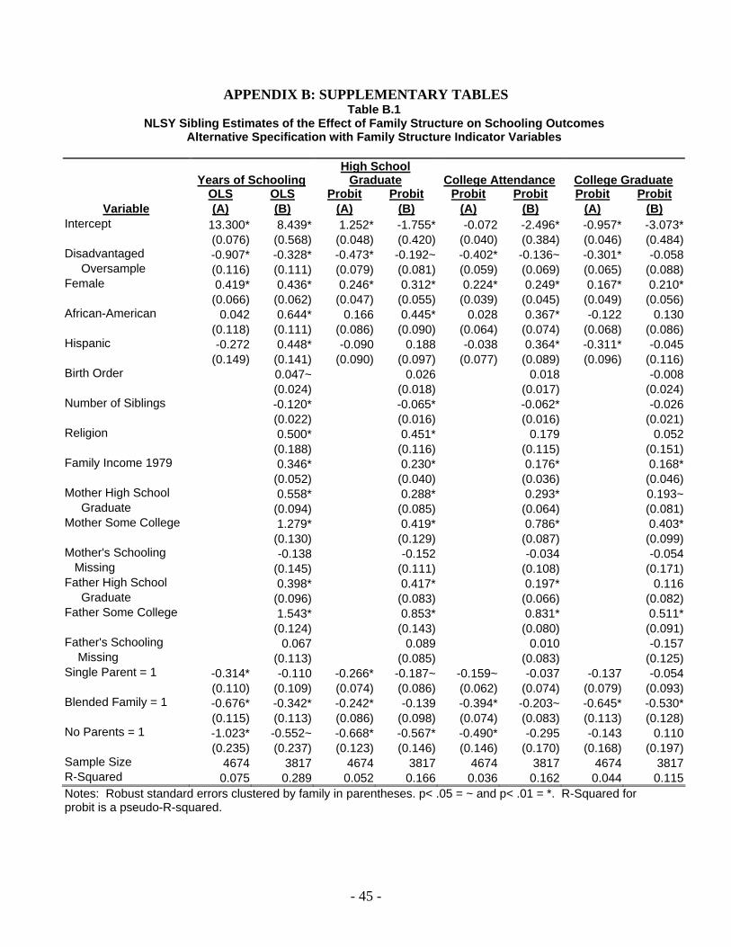
- 45 -

APPENDIX B: SUPPLEMENTARY TABLES Table B.1

NLSY Sibling Estimates of the Effect of Family Structure on Schooling Outcomes Alternative Specification with Family Structure Indicator Variables

Years of Schooling High School

Graduate

College Attendance

College Graduate OLS OLS Probit Probit Probit Probit Probit Probit

Variable (A) (B) (A) (B) (A) (B) (A) (B) Intercept 13.300* 8.439* 1.252* -1.755* -0.072 -2.496* -0.957* -3.073*

(0.076) (0.568) (0.048) (0.420) (0.040) (0.384) (0.046) (0.484)Disadvantaged -0.907* -0.328* -0.473* -0.192~ -0.402* -0.136~ -0.301* -0.058 Oversample (0.116) (0.111) (0.079) (0.081) (0.059) (0.069) (0.065) (0.088)Female 0.419* 0.436* 0.246* 0.312* 0.224* 0.249* 0.167* 0.210*

(0.066) (0.062) (0.047) (0.055) (0.039) (0.045) (0.049) (0.056)African-American 0.042 0.644* 0.166 0.445* 0.028 0.367* -0.122 0.130

(0.118) (0.111) (0.086) (0.090) (0.064) (0.074) (0.068) (0.086)Hispanic -0.272 0.448* -0.090 0.188 -0.038 0.364* -0.311* -0.045

(0.149) (0.141) (0.090) (0.097) (0.077) (0.089) (0.096) (0.116)Birth Order 0.047~ 0.026 0.018 -0.008

(0.024) (0.018) (0.017) (0.024)Number of Siblings -0.120* -0.065* -0.062* -0.026

(0.022) (0.016) (0.016) (0.021)Religion 0.500* 0.451* 0.179 0.052

(0.188) (0.116) (0.115) (0.151)Family Income 1979 0.346* 0.230* 0.176* 0.168*

(0.052) (0.040) (0.036) (0.046)Mother High School 0.558* 0.288* 0.293* 0.193~ Graduate (0.094) (0.085) (0.064) (0.081)Mother Some College 1.279* 0.419* 0.786* 0.403*

(0.130) (0.129) (0.087) (0.099)Mother's Schooling -0.138 -0.152 -0.034 -0.054 Missing (0.145) (0.111) (0.108) (0.171)Father High School 0.398* 0.417* 0.197* 0.116 Graduate (0.096) (0.083) (0.066) (0.082)Father Some College 1.543* 0.853* 0.831* 0.511* (0.124) (0.143) (0.080) (0.091)Father's Schooling 0.067 0.089 0.010 -0.157 Missing (0.113) (0.085) (0.083) (0.125)Single Parent = 1 -0.314* -0.110 -0.266* -0.187~ -0.159~ -0.037 -0.137 -0.054 (0.110) (0.109) (0.074) (0.086) (0.062) (0.074) (0.079) (0.093)Blended Family = 1 -0.676* -0.342* -0.242* -0.139 -0.394* -0.203~ -0.645* -0.530* (0.115) (0.113) (0.086) (0.098) (0.074) (0.083) (0.113) (0.128)No Parents = 1 -1.023* -0.552~ -0.668* -0.567* -0.490* -0.295 -0.143 0.110 (0.235) (0.237) (0.123) (0.146) (0.146) (0.170) (0.168) (0.197)Sample Size 4674 3817 4674 3817 4674 3817 4674 3817R-Squared 0.075 0.289 0.052 0.166 0.036 0.162 0.044 0.115Notes: Robust standard errors clustered by family in parentheses. p< .05 = ~ and p< .01 = *. R-Squared for probit is a pseudo-R-squared.

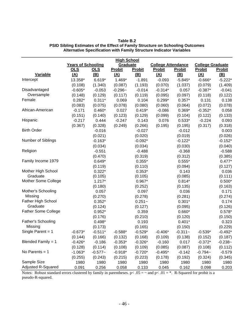
- 46 -

Table B.2 PSID Sibling Estimates of the Effect of Family Structure on Schooling Outcomes

Alternative Specification with Family Structure Indicator Variables

Years of Schooling

High School Graduate

College Attendance

College Graduate

OLS OLS Probit Probit Probit Probit Probit Probit Variable (A) (B) (A) (B) (A) (B) (A) (B)

Intercept 13.358* 6.619* 1.469* -1.891 -0.093 -5.845* -0.666* -5.222* (0.108) (1.340) (0.087) (1.193) (0.070) (1.037) (0.079) (1.409)

Disadvantaged -0.605* -0.053 -0.296~ -0.014 -0.314* 0.057 -0.387* -0.041 Oversample (0.148) (0.129) (0.117) (0.119) (0.095) (0.097) (0.118) (0.122)Female 0.282* 0.311* 0.069 0.104 0.299* 0.357* 0.131 0.138

(0.083) (0.075) (0.078) (0.080) (0.060) (0.064) (0.072) (0.078)African-American -0.171 0.460* 0.027 0.419* -0.086 0.369* -0.352* 0.058

(0.151) (0.140) (0.123) (0.129) (0.099) (0.104) (0.122) (0.133)Hispanic -0.217 0.444 -0.247 0.143 0.076 0.533* -0.224 0.093

(0.367) (0.328) (0.249) (0.266) (0.195) (0.195) (0.317) (0.318)Birth Order -0.016 -0.027 -0.012 0.003

(0.021) (0.020) (0.019) (0.026)Number of Siblings -0.163* -0.092* -0.122* -0.152*

(0.034) (0.034) (0.030) (0.040)Religion -0.551 -0.488 -0.368 -0.588

(0.470) (0.319) (0.312) (0.385)Family Income 1979 0.649* 0.355* 0.555* 0.477*

(0.119) (0.110) (0.094) (0.127)Mother High School 0.322* 0.353* 0.143 0.036 Graduate (0.105) (0.105) (0.085) (0.111)Mother Some College 1.217* 0.967* 0.814* 0.500*

(0.180) (0.252) (0.135) (0.163)Mother's Schooling 0.057 0.097 0.036 0.171 Missing (0.270) (0.278) (0.281) (0.274)Father High School 0.352* 0.251~ 0.301* 0.174 Graduate (0.124) (0.127) (0.095) (0.126)Father Some College 0.952* 0.359 0.660* 0.578* (0.176) (0.210) (0.120) (0.150)Father's Schooling 0.498* 0.193 0.401* 0.323 Missing (0.173) (0.165) (0.150) (0.229)Single Parent = 1 -0.673* -0.511* -0.588* -0.529* -0.406* -0.311~ -0.539* -0.492* (0.144) (0.166) (0.132) (0.168) (0.109) (0.138) (0.152) (0.187)Blended Family = 1 -0.426* -0.186 -0.353* -0.326* -0.160 0.017 -0.372* -0.238~ (0.128) (0.114) (0.108) (0.109) (0.085) (0.087) (0.108) (0.112)No Parents = 1 -1.063* -0.577~ -0.918* -0.720* -0.495* -0.142 -0.794~ -0.579 (0.255) (0.243) (0.215) (0.223) (0.178) (0.192) (0.324) (0.345)Sample Size 1980 1980 1980 1980 1980 1980 1980 1980Adjusted R-Squared 0.091 0.256 0.058 0.133 0.045 0.162 0.098 0.203Notes: Robust standard errors clustered by family in parentheses. p< .05 = ~ and p< .01 = *. R-Squared for probit is a pseudo-R-squared.

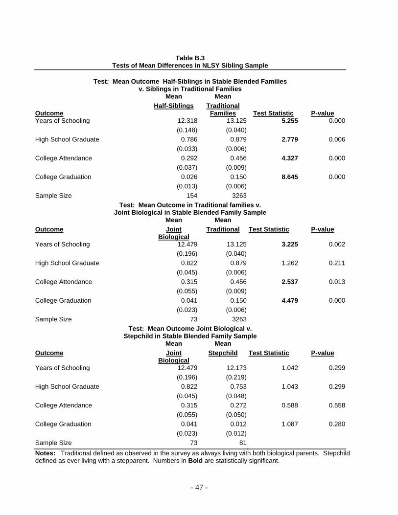
- 47 -

Table B.3

Tests of Mean Differences in NLSY Sibling Sample

Test: Mean Outcome Half-Siblings in Stable Blended Families v. Siblings in Traditional Families

Mean Mean Outcome

Half-Siblings Traditional Families

Test Statistic

P-value

Years of Schooling 12.318 13.125 5.255 0.000 (0.148) (0.040) High School Graduate 0.786 0.879 2.779 0.006 (0.033) (0.006) College Attendance 0.292 0.456 4.327 0.000 (0.037) (0.009) College Graduation 0.026 0.150 8.645 0.000 (0.013) (0.006) Sample Size 154 3263

Test: Mean Outcome in Traditional families v. Joint Biological in Stable Blended Family Sample

Mean Mean Outcome Joint

Biological Traditional Test Statistic P-value

Years of Schooling 12.479 13.125 3.225 0.002 (0.196) (0.040) High School Graduate 0.822 0.879 1.262 0.211 (0.045) (0.006) College Attendance 0.315 0.456 2.537 0.013 (0.055) (0.009) College Graduation 0.041 0.150 4.479 0.000 (0.023) (0.006) Sample Size 73 3263

Test: Mean Outcome Joint Biological v. Stepchild in Stable Blended Family Sample

Mean Mean Outcome Joint

Biological Stepchild Test Statistic P-value

Years of Schooling 12.479 12.173 1.042 0.299 (0.196) (0.219) High School Graduate 0.822 0.753 1.043 0.299 (0.045) (0.048) College Attendance 0.315 0.272 0.588 0.558 (0.055) (0.050) College Graduation 0.041 0.012 1.087 0.280 (0.023) (0.012) Sample Size 73 81 Notes: Traditional defined as observed in the survey as always living with both biological parents. Stepchild defined as ever living with a stepparent. Numbers in Bold are statistically significant.

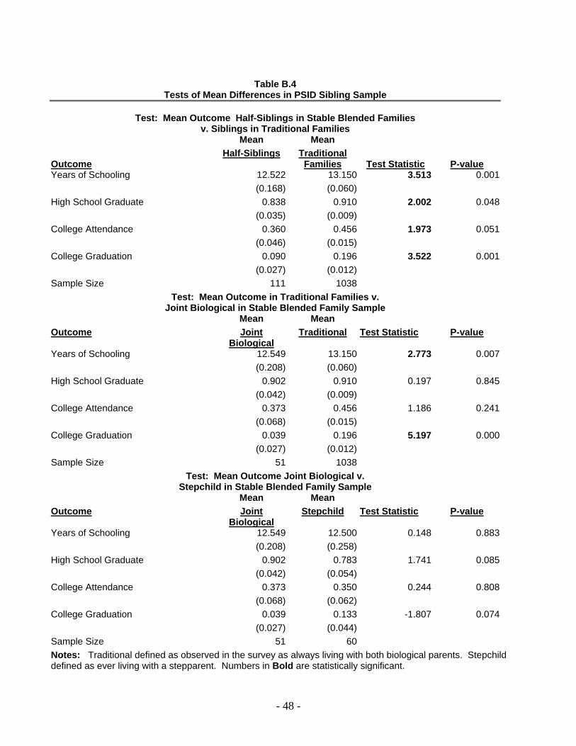
- 48 -

Table B.4

Tests of Mean Differences in PSID Sibling Sample

Test: Mean Outcome Half-Siblings in Stable Blended Families v. Siblings in Traditional Families

Mean Mean Outcome

Half-Siblings Traditional Families

Test Statistic

P-value

Years of Schooling 12.522 13.150 3.513 0.001 (0.168) (0.060) High School Graduate 0.838 0.910 2.002 0.048 (0.035) (0.009) College Attendance 0.360 0.456 1.973 0.051 (0.046) (0.015) College Graduation 0.090 0.196 3.522 0.001 (0.027) (0.012) Sample Size 111 1038

Test: Mean Outcome in Traditional Families v. Joint Biological in Stable Blended Family Sample

Mean Mean Outcome Joint

Biological Traditional Test Statistic P-value

Years of Schooling 12.549 13.150 2.773 0.007 (0.208) (0.060) High School Graduate 0.902 0.910 0.197 0.845 (0.042) (0.009) College Attendance 0.373 0.456 1.186 0.241 (0.068) (0.015) College Graduation 0.039 0.196 5.197 0.000 (0.027) (0.012) Sample Size 51 1038

Test: Mean Outcome Joint Biological v. Stepchild in Stable Blended Family Sample

Mean Mean Outcome Joint

Biological Stepchild Test Statistic P-value

Years of Schooling 12.549 12.500 0.148 0.883 (0.208) (0.258) High School Graduate 0.902 0.783 1.741 0.085 (0.042) (0.054) College Attendance 0.373 0.350 0.244 0.808 (0.068) (0.062) College Graduation 0.039 0.133 -1.807 0.074 (0.027) (0.044) Sample Size 51 60 Notes: Traditional defined as observed in the survey as always living with both biological parents. Stepchild defined as ever living with a stepparent. Numbers in Bold are statistically significant.

- 49 -

Table B.5

NLSY Blended Family Sample Estimates of the Effect of Family Structure on Educational Outcomes

Years of Schooling

High School

Graduate

College Attendance OLS OLS Probit Probit Probit Probit

Variable (A) (B) (A) (B) (A) (B) Intercept 11.918* 10.704* 0.793* 0.074 -0.910* -1.314*

(0.378) (0.758) (0.294) (0.597) (0.283) (0.444) Disadvantaged 0.119 0.095 -0.023 0.038 0.130 0.122 Oversample (0.344) (0.353) (0.351) (0.321) (0.320) (0.331) Female 0.423 0.331 0.167 0.090 0.488~ 0.561~

(0.285) (0.296) (0.206) (0.243) (0.221) (0.238) African-American 0.593 0.681 0.262 0.450 0.247 0.379

(0.424) (0.372) (0.392) (0.387) (0.353) (0.374) Hispanic 0.403 0.445 -0.375 -0.431 0.169 0.258

(0.717) (0.733) (0.489) (0.485) (0.519) (0.533) Birth Order 0.138 0.180 0.076

(0.106) (0.098) (0.073) Number of Siblings -0.057 -0.061 -0.046

(0.084) (0.080) (0.075) Religion 0.738 0.309

(0.528) (0.477) Mother High School -0.160 -0.071 0.019 Graduate (0.390) (0.315) (0.325) Mother Some College 0.941 0.141 1.230*

(0.561) (0.448) (0.426) Mother's Schooling -0.089 -0.364 0.625 Missing (0.792) (0.637) (0.563) Father High School 0.594 0.366 0.266 Graduate (0.389) (0.360) (0.285) Father Some 1.348~ 0.803 College (0.563) (0.416) Father's Schooling 0.069 -0.326 -0.026 Missing (0.388) (0.336) (0.370) Proportion in -0.665 -0.602 -0.406 -0.350 -0.325 -0.377 Non-intact Family (0.364) (0.386) (0.231) (0.272) (0.261) (0.306) Sample Size 154 154 154 139 154 143 Adjusted R-Squared 0.06 0.165 0.037 0.111 0.045 0.123 Notes: Robust standard errors clustered by family in parentheses. p< .05 = ~ and p< .01 = *. R-Squared for probit is a pseudo-R-squared. Some variables and observations are omitted from Model (B) because their inclusion predicts the outcome perfectly.

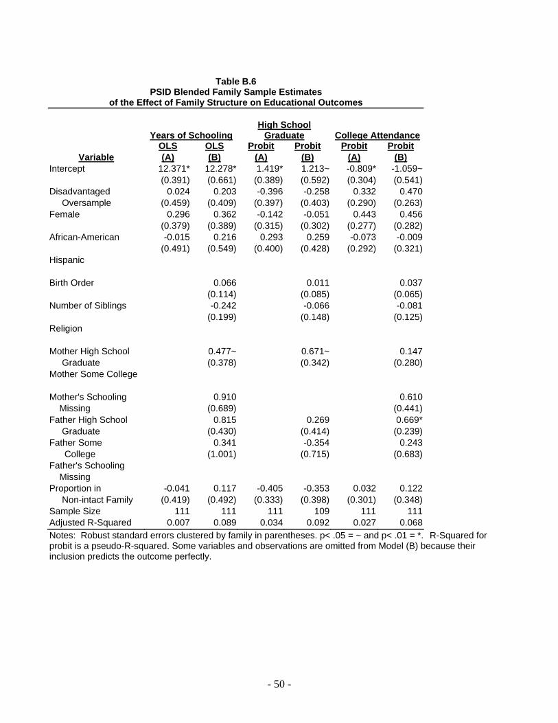
- 50 -

Table B.6

PSID Blended Family Sample Estimates of the Effect of Family Structure on Educational Outcomes

Years of Schooling

High School

Graduate

College Attendance OLS OLS Probit Probit Probit Probit

Variable (A) (B) (A) (B) (A) (B) Intercept 12.371* 12.278* 1.419* 1.213~ -0.809* -1.059~

(0.391) (0.661) (0.389) (0.592) (0.304) (0.541) Disadvantaged 0.024 0.203 -0.396 -0.258 0.332 0.470 Oversample (0.459) (0.409) (0.397) (0.403) (0.290) (0.263) Female 0.296 0.362 -0.142 -0.051 0.443 0.456

(0.379) (0.389) (0.315) (0.302) (0.277) (0.282) African-American -0.015 0.216 0.293 0.259 -0.073 -0.009

(0.491) (0.549) (0.400) (0.428) (0.292) (0.321) Hispanic

Birth Order 0.066 0.011 0.037

(0.114) (0.085) (0.065) Number of Siblings -0.242 -0.066 -0.081

(0.199) (0.148) (0.125) Religion

Mother High School 0.477~ 0.671~ 0.147 Graduate (0.378) (0.342) (0.280) Mother Some College

Mother's Schooling 0.910 0.610 Missing (0.689) (0.441) Father High School 0.815 0.269 0.669* Graduate (0.430) (0.414) (0.239) Father Some 0.341 -0.354 0.243 College (1.001) (0.715) (0.683) Father's Schooling Missing Proportion in -0.041 0.117 -0.405 -0.353 0.032 0.122 Non-intact Family (0.419) (0.492) (0.333) (0.398) (0.301) (0.348) Sample Size 111 111 111 109 111 111 Adjusted R-Squared 0.007 0.089 0.034 0.092 0.027 0.068 Notes: Robust standard errors clustered by family in parentheses. p< .05 = ~ and p< .01 = *. R-Squared for probit is a pseudo-R-squared. Some variables and observations are omitted from Model (B) because their inclusion predicts the outcome perfectly.