Family spending in the UK

Page 1 of 88

Next release: 8 December 2015

Release date: 2 December 2014

Contact: Giles Horsfield [email protected] +44 (0)1633 455678

Compendium

Family spending in the UK: calendar year 2013Average weekly household expenditure on goods and services in the UK, by region, age, income, economic status, socio-economic class and household composition.

Chapters in this compendium

1. About this edition

2. Chapter 1: Overview

3. Chapter 2: Housing expenditure

4. Chapter 3: Equivalised income

5. Chapter 4: Trends in household expenditure over time

6. Survey methodology: Appendix B

https://www.statisticsauthority.gov.uk/national-statistician/types-of-official-statistics/

Page 2 of 88

Next release: To be announced



Compendium

About this editionA report on the Living Costs and Food Survey 2013, including spending on housing, utilities and other outgoings.

Table of contents

1. Abstract

2. Acknowledgements

3. List of contributors

4. Introduction

5. Background notes


Page 3 of 88

1 . Abstract

This report presents the latest information from the Living Costs and Food Survey for the 2013 calendar year (January to December). The Expenditure and Food Survey (EFS) was renamed as the Living Costs and Food Survey (LCF) in 2008 when it became a module of the Integrated Household Survey (IHS).

2 . Acknowledgements

A large scale survey is a collaborative effort and the authors wish to thank the interviewers and other ONS staff who contributed to the study. The survey would not be possible without the co-operation of the respondents who gave up their time to be interviewed and keep a diary of their spending. Their help is gratefully acknowledged.

3 . List of contributors

Authors:

Joanna Bulman Laura Dimond Rachael Ryan Rhian Jones

Living Costs and Food Survey team:

Jana Kubascikova-Mullen Linda Williams Michelle Cooper Paul Bloomfield Sarah Whiting Tracy Lane

Field Team and Interviewers Coders and Editors

Review and additional commentary:

Chris Daffin David Matthewson Richard Tonkin Yanitsa Petkova

4 . Introduction

This report presents the latest information from the Living Costs and Food Survey for the 2013 calendar year (January to December). The Expenditure and Food Survey (EFS) was renamed as the Living Costs and Food Survey (LCF) in 2008 when it became a module of the Integrated Household Survey (IHS).

The current LCF is the result of the amalgamation of the Family Expenditure and National Food Surveys (FES and NFS). Both surveys were well established and important sources of information for government and the wider community, charting changes and patterns in Britain’s spending and food consumption since the 1950s. The Office for National Statistics (ONS) has overall project management and financial responsibility for the LCF while the Department for Environment, Food and Rural Affairs (DEFRA) sponsors the specialist food data.

The survey continues to be used primarily to provide information for the Consumer Prices Index and the Retail Prices Index; National Accounts estimates of household expenditure; the analysis of the effect of taxes and benefits; and trends in nutrition. However, the results are multi purpose, providing an invaluable supply of economic and social data.

Page 4 of 88

The 2013 survey

In 2013 4,993 households in Great Britain took part in the LCF survey. The response rate was 48% in Great Britain and 61% in Northern Ireland. The fieldwork was undertaken by the Office for National Statistics and the Northern Ireland Statistics and Research Agency (NISRA). Further details about the conduct of the survey are given in Appendix B.

This year’s report includes an overview chapter outlining key findings, and detailed chapters focusing upon expenditure on housing, patterns of spending by equivalised income and trends in household expenditure over time.

Data quality and definitions

The results shown in this report are of the data collected by the LCF, following a process of validation and adjustment for non-response using weights that control for a number of factors. These issues are discussed in the section on reliability in .Appendix B

Figures in the report are subject to sampling variability. Standard errors for detailed expenditure items are presented in relative terms in and are described in . Figures shown table A1 (153.5 Kb Excel sheet) Appendix Bfor particular groups of households (for example income groups or household composition groups), regions or other sub-sets of the sample are subject to larger sampling variability, and are more sensitive to possible extreme values than are figures for the sample as a whole.

The definitions used in the report are set out in , and changes made since 1991 are described in the Appendix BTechnical Report. Note particularly that housing benefit and council tax rebate (rates rebate in Northern Ireland), unlike other social security benefits, are not included in income but are shown as a reduction in housing costs.

Income and expenditure balancing

The LCF is designed primarily as a survey of household expenditure on goods and services. It also gathers information about the income of household members, and is an important and detailed source of income data. However, the survey is not designed to produce a balance sheet of income and expenditure either for individual households or groups of households. For further information on the balancing of income and expenditure figures, see 'Response to the survey’, .Appendix B

Related data sources

Details of household consumption expenditure within the context of the UK National Accounts are produced as part of . This publication includes all expenditure by members of UK resident households. Consumer TrendsNational Accounts figures draw on a number of sources including the LCF: figures shown in this report are therefore not directly comparable to National Accounts data. National Accounts data may be more appropriate for deriving long term trends on expenditure.

More detailed income information is available from the Family Resources Survey (FRS), conducted for the Department for Work and Pensions. Further information about food consumption, and in particular details of food quantities, is available from the Department for Environment, Food and Rural Affairs, who produce their own

of the survey.report

http://www.ons.gov.uk/ons/rel/family-spending/family-spending/2014-edition/art-survey-methodology-appendix-b.html

http://www.ons.gov.uk/ons/rel/family-spending/family-spending/2014-edition/rft-table-a1.xls




http://www.ons.gov.uk/ons/rel/consumer-trends/consumer-trends/index.html

http://www.defra.gov.uk/statistics/foodfarm/food/familyfood/

http://www.defra.gov.uk/statistics/foodfarm/food/familyfood/

Page 5 of 88

1.

2.

3.

Additional tabulations

This report gives a broad overview of the results of the survey, and provides more detailed information about some aspects of expenditure. However, many users of LCF data have very specific data requirements that may not appear in the desired form in this report. ONS can provide more detailed analysis of the tables in this report, and can also provide additional tabulations to meet specific requests. A charge will be made to cover the cost of providing additional information.

The tables in Family Spending 2014 are available as Excel spreadsheets.

Anonymised microdata from the Living Costs and Food Survey (LCF), the Expenditure and Food Survey (EFS) and the Family Expenditure Survey (FES) are available from the United Kingdom Data Service. Details on access arrangements and associated costs can be found at or by telephoning 01206 872143.http://ukdataservice.ac.uk/

5. Background notes

Symbols and conventions used in Family Spending 2014 edition

[ ] Figures should be used with extra caution because they are based on fewer than 20 reporting households.

.. The data is suppressed if the unweighted sample counts are less than 10 reporting households.

- No figures are available because there are no reporting households.

Rounding: Individual figures have been rounded independently. The sum of component items does not therefore necessarily add to the totals shown.

Averages: These are averages (means) for all households included in the column or row, and unless specified, are not restricted to those households reporting expenditure on a particular item or income of a particular type.

Period covered: Calendar year 2013 (1 January 2013 to 31 December 2013).

Contacts

For information about the content of this publication, contact ONS Social Surveys Data Advice and Relations Team.

Tel +44 (0)1633 455678 Email: [email protected]

Other customer enquiries

ONS Customer Contact Centre Tel: 0845 601 3034 International: +44 (0) 1633 817521 Minicom: +44 (0)1633 815044 Email: Fax: +44 (0)1633 [email protected]

Post: Room D265, Government Buildings, Cardiff Road, Newport, South Wales NP10 8XG www.ons.gov.uk

Media enquiries

Tel: +44 (0)845 604 1858 Email: [email protected]

Editor

Giles Horsfield [email protected]

A National Statistics publication

National Statistics are produced to high professional standards set out in the Code of Practice for Official . They are produced free from political influence.Statistics

http://ukdataservice.ac.uk/

http://www.ons.gov.uk/

http://www.ons.gov.uk/ons/guide-method/the-national-statistics-standard/code-of-practice/index.html


Page 6 of 88




4.

5.

6.

About us

The Office for National Statistics

The Office for National Statistics (ONS) is the executive office of the , a non-UK Statistics Authorityministerial department which reports directly to Parliament. ONS is the UK government’s single largest statistical producer. It compiles information about the UK’s society and economy, and provides the evidence-base for policy and decision-making, the allocation of resources, and public accountability. The Director-General of ONS reports directly to the National Statistician who is the Authority's Chief Executive and the Head of the Government Statistical Service.

The Government Statistical Service

The Government Statistical Service (GSS) is a network of professional statisticians and their staff operating both within the Office for National Statistics and across more than 30 other government departments and agencies.

Copyright and reproduction

© Crown copyright 2014

Under the terms of the and UK Government Licensing Framework, anyone Open Government Licencewishing to use or re-use ONS material, whether commercially or privately, may do so freely without a specific application for a licence, subject to the conditions of the OGL and the Framework.

For further information, contact the Office of Public Sector Information, Crown Copyright Licensing and Public Sector Information, Kew, Richmond, Surrey, TW9 4DU.

Tel: +44 (0)20 8876 3444

Email: [email protected]

ISSN 2040-1647

Details of the policy governing the release of new data are available by visiting www.statisticsauthority.gov. or from the Media Relations Office email: uk/assessment/code-of-practice/index.html media.relations@ons.

gsi.gov.uk

These National Statistics are produced to high professional standards and released according to the arrangements approved by the UK Statistics Authority.

Compendium

Chapter 1: OverviewA report on the Living Costs and Food Survey 2013, including spending on housing, utilities and other outgoings.


http://www.ons.gov.uk/ons/external-links/stats-authority/statistics-authority-s-website.html

http://www.ons.gov.uk/ons/external-links/other-government-departments/national-archives/index.html

http://www.statisticsauthority.gov.uk/assessment/code-of-practice/index.html


Page 7 of 88

Table of contents

1. Abstract

2. Key points

3. Household expenditure in 2013

4. Trends in spending over time

5. Expenditure by region

6. Income

7. Computer ownership and internet connection at home

8. Background notes

Page 8 of 88

1.

1 . Abstract

This chapter presents the key findings of the 2013 Living Costs and Food Survey (LCF). The overview covers: expenditure in 2013; trends in spending over time; expenditure in different areas of the UK; expenditure by income group; ownership of home computers and access to the internet at home. Some of these topics are explored in more depth in the publication. Links are provided to the sections of Family Spending that contain the detailed coverage.

2 . Key points

Total average weekly household expenditure was £517.30 in 2013.

Housing (net), fuel and power had the highest average spending in 2013, at £74.40 per week, accounting for 14% for household spending, on average. This category excludes mortgage payments.

Transport was the second highest-spending category, at £70.40 per week, on average.

Average spending decreased between 2006 and 2013, once the figures have been adjusted to allow for changes in prices (inflation).

Households in the South East and London spend the most, while those in the North East spend the least.

Expenditure in rural areas was higher than in urban areas

Spending is presented using Classification Of Individual COnsumption by Purpose (COICOP) categories, unless 1

stated otherwise. COICOP is an internationally-recognised classification system, consistent with that used by UK National Accounts. It does not include all types of payments, and some types of housing-related expenses, such as mortgage payments, are excluded. However, due to the high interest in the topic, chapter 2 provides a detailed analysis of housing-related expenditure, including the items not included under COICOP.

Notes for key points

From 2001, the Classification Of Individual COnsumption by Purpose (COICOP) was introduced as a new coding frame for expenditure items. COICOP is the internationally agreed classification system for reporting household consumption expenditure. Total expenditure is made up from the total of the COICOP expenditure groups (1 to 12) plus ‘Other expenditure items (13)’. Other expenditure items are those items excluded from the COICOP categories, such as mortgage interest payments, council tax, domestic rates, holiday spending, cash gifts and charitable donations.

3 . Household expenditure in 2013

Table 1.1 shows average weekly household expenditure in the United Kingdom (UK) by the 12 COICOP categories. In 2013, average weekly household expenditure in the UK was £517.30.

Page 9 of 88

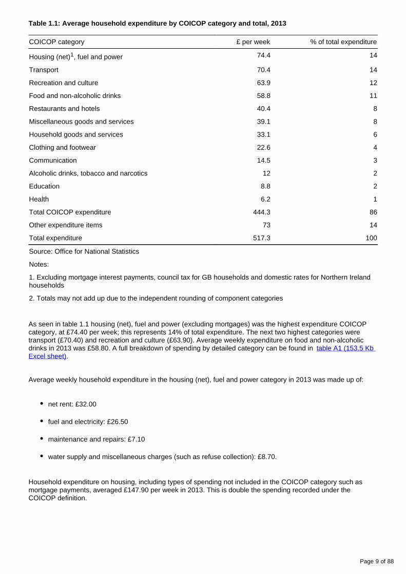
Table 1.1: Average household expenditure by COICOP category and total, 2013

COICOP category £ per week % of total expenditure

Housing (net) , fuel and power1 74.4 14

Transport 70.4 14

Recreation and culture 63.9 12

Food and non-alcoholic drinks 58.8 11

Restaurants and hotels 40.4 8

Miscellaneous goods and services 39.1 8

Household goods and services 33.1 6

Clothing and footwear 22.6 4

Communication 14.5 3

Alcoholic drinks, tobacco and narcotics 12 2

Education 8.8 2

Health 6.2 1

Total COICOP expenditure 444.3 86

Other expenditure items 73 14

Total expenditure 517.3 100

Source: Office for National Statistics

Notes:

1. Excluding mortgage interest payments, council tax for GB households and domestic rates for Northern Ireland households

2. Totals may not add up due to the independent rounding of component categories

As seen in table 1.1 housing (net), fuel and power (excluding mortgages) was the highest expenditure COICOP category, at £74.40 per week; this represents 14% of total expenditure. The next two highest categories were transport (£70.40) and recreation and culture (£63.90). Average weekly expenditure on food and non-alcoholic drinks in 2013 was £58.80. A full breakdown of spending by detailed category can be found in table A1 (153.5 Kb

.Excel sheet)

Average weekly household expenditure in the housing (net), fuel and power category in 2013 was made up of:

net rent: £32.00

fuel and electricity: £26.50

maintenance and repairs: £7.10

water supply and miscellaneous charges (such as refuse collection): £8.70.

Household expenditure on housing, including types of spending not included in the COICOP category such as mortgage payments, averaged £147.90 per week in 2013. This is double the spending recorded under the COICOP definition.



Page 10 of 88

Unless otherwise stated, figures in this report are averaged across all households. This means, for example, that average weekly expenditure on buying vehicles is averaged across all households, whether or not they bought a vehicle. The exception, where stated, is for spending on rent and mortgages, where spending is also presented only for households that pay mortgages, or rent, respectively. Considering only households that pay mortgages, average weekly expenditure on mortgages was £145.40. Spending on net rent, for households that rented their accommodation, averaged £92.10 per week. These are the only spending figures in family spending that are not averaged across all households. ‘Net rent’ refers to the rent paid by the householders themselves, so any rebates and allowances (including housing benefit) are excluded from the total.

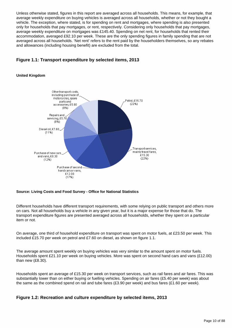
Figure 1.1: Transport expenditure by selected items, 2013

United Kingdom

Source: Living Costs and Food Survey - Office for National Statistics

Different households have different transport requirements, with some relying on public transport and others more on cars. Not all households buy a vehicle in any given year, but it is a major expense for those that do. The transport expenditure figures are presented averaged across all households, whether they spent on a particular item or not.

On average, one third of household expenditure on transport was spent on motor fuels, at £23.50 per week. This included £15.70 per week on petrol and £7.60 on diesel, as shown on figure 1.1.

The average amount spent weekly on buying vehicles was very similar to the amount spent on motor fuels. Households spent £21.10 per week on buying vehicles. More was spent on second hand cars and vans (£12.00) than new (£8.30).

Households spent an average of £15.30 per week on transport services, such as rail fares and air fares. This was substantially lower than on either buying or fuelling vehicles. Spending on air fares (£5.40 per week) was about the same as the combined spend on rail and tube fares (£3.90 per week) and bus fares (£1.60 per week).

Figure 1.2: Recreation and culture expenditure by selected items, 2013

Page 11 of 88

United Kingdom


Expenditure within the recreation and culture category represents a broad range of goods and services. An important part of the spending in this area is the sub-category recreational and cultural services, which accounted for £18.60 per week. There is a wide range of choice available in this area, including:

sports admissions, subscriptions, leisure class fees and equipment hire (£5.50)

cinema, theatre and museums etc (£2.30)

TV subscriptions and licences (£6.70).

Expenditure on package holidays averaged £22.40 per week; this includes both domestic and foreign holidays.

Also within recreation and culture, an average of £4.30 per week was spent on pets and pet food, and £2.30 on games, toys and hobbies.

The fourth highest category of household spending was food and non-alcoholic drinks, averaging £58.80 per week. A similar amount was spent on bread, rice and cereals (£5.60 per week) and non-alcoholic drinks (£4.90 per week); this compares with £4.30 per week on fresh vegetables and £3.30 on fresh fruit.

4 . Trends in spending over time

In spending figures over time are adjusted to take account of inflation. This enables a comparison of chapter 4expenditure to be made between survey years that allows for changing prices.

http://www.ons.gov.uk/ons/rel/family-spending/family-spending/2014-edition/art-chapter-4.html

Page 12 of 88

Household average weekly expenditure has decreased since 2006, once inflation has been taken into account. Average weekly household spending was £539.80 in 2006, and started declining, just before the economic downturn, in 2007 (when £531.70 per week was recorded). Average spending decreased further to £501.00 in 2012, and then increased to £517.30 in 2013 . Between 2001/2 and 2006, average expenditure was at a higher 1

level than that seen since 2006.

The trends observed in total household spending after 2008 are broadly consistent with the wider economic context. This is explored in more detail in .chapter 4

Not all types of household spending have decreased in recent years. Spending on housing (net), fuel and power increased from £61.70 in 2001/2, to £74.40 in 2013, after adjusting for inflation. Rent payments make up the largest proportion of expenditure in this category. The number of households renting accommodation has increased over recent years, as shown in for 2013, and the corresponding table for table A50 (50 Kb Excel sheet)2006. These tables show the proportion of households renting increased, from 29% in 2006, to 35% in 2013. Therefore, the increased proportion of households renting has contributed to higher spending on housing (net), fuel and power.

Average household spending on transport decreased between 2001/2 (adjusted to 2013 prices) and 2013. However, it increased to £70.40 in 2013, from £64.80 per week in 2012. Households allocated an average of 14% of total expenditure to transport in 2013.

Higher average household expenditure on transport between 2012 and 2013 can partly be attributed to an increase of new car purchases. Vehicle purchases were recorded as being at a six-year high with 1,074,622 new private . Purchasing new cars is an area where households could moderate or defer expenditure, cars registeredwhich may lead to demand building up over time. This is sometimes referred to as “pent up demand”. This may have fuelled the increase in sales of new cars seen in 2013, with consumers replacing vehicles they kept hold of through the recent downturn.

Recent years have seen the price of petrol and diesel increase substantially, with costs rising above the overall rate of inflation in 2012. However, between 2012 and 2013 , so the increase in transport prices decreased slightlyexpenditure in 2013 cannot be attributed to spending on fuel.


http://www.ons.gov.uk/ons/rel/family-spending/family-spending/2014-edition/rft-a50-final-2013.xls

http://www.smmt.co.uk/2014/01/2013-new-car-market-records-best-performance-five-years

https://www.gov.uk/government/statistical-data-sets/oil-and-petroleum-products-monthly-statistics

Page 13 of 88

1.

2.

3.

Figure 1.3: Expenditure on selected categories based on COICOP classification, 2001-02 to 2013, at 2013 prices


Notes:

Figures have been deflated to 2013 prices using deflators specific to the COICOP category

In 2006, Family Spending changed to report for a calendar year instead of a financial year

From 2001-02 to 2005-06, figures shown are calculated from weighted data using non-response weights based on the 1991 Census and population figures from the 1991 and 2001 Censuses. From 2006 onwards, figures shown are calculated from weighted data using non-response weights and population figures based on the 2001 Census

Spending on transport; housing (net), fuel and power; recreation and culture; food and non-alcoholic drink; and hotels and restaurants over the years 2001/2 to 2013 are shown in figure 1.3. The figures are adjusted for inflation, and shown at 2013 prices. The chart shows the different trends in spending for these categories over this period.

Notes for trends in spending over time

Page 14 of 88

1. This increase was not found to be significant at the 95% confidence level.

5 . Expenditure by region

Figure 1.4: Household expenditure by region, 2011 to 2013

United Kingdom


Three years' data are combined when presenting spending figures broken down by country and region. This ensures the sample size is large enough to provide robust figures when below-UK levels of geography are considered. Detailed expenditure by region is shown in .table A35 (103 Kb Excel sheet)

The average weekly household expenditure in the UK combined over the years 2011 to 2013 was £496.70. Four regions showed expenditure higher than the UK average; the two highest-spending regions, the South East and London, recorded very similar levels of expenditure. In descending order the top four regions are: the South East (£585.40), London (£579.60), the East (£523.40) and the South West (£518.20). At the opposite end of the scale with the lowest average expenditure are the North East (£424.60), Yorkshire and the Humber (£431.10) and Wales (£438.80). Average weekly expenditure in Scotland was £449.00.

For the three-year period 2011 to 2013, London was the highest spending region on housing (net), fuel and power (excluding mortgage payments), by a sizeable margin, at £103.20 per week, compared with the second highest average expenditure of £74.80 in the South East. As for previous years the major factor in London’s large expenditure was net rent, at £62.50 per week. This was nearly twice the amount of the South East (£31.50); the second highest expenditure region on rent. Expenditure on rent is averaged across all households, including those that don’t pay rent, so the higher rent figures for London reflect both the higher costs of rent, and the high proportion of householders who rent their accommodation.

http://www.ons.gov.uk/ons/resources/figure14final2013_tcm77-385864.png


Page 15 of 88

Transport spending in the UK averaged £66.80 over the years 2011 to 2013. It was notably higher in the South East, at £84.50 per week. London’s households spent lower than the UK average on transport, at £62.50 per week. London’s relatively low spending on transport was most striking in operation of personal transport (fuel and running costs of vehicles), where London was the lowest spending area at £25.30 per week, compared with the UK average of £35.60. As a general pattern across the UK, expenditure on the purchase of new vehicles is almost double that spent on transport services such as train and bus fares. However, London reported a notably larger expenditure on transport services (£22.60) than new vehicles (£14.60). This lower expenditure on the purchase of new vehicles is reflected by the fact that only 61% of households owned a car/van in London over the years 2011 to 2013, compared to 75% of households in the UK as a whole (see table A48 (69.5 Kb Excel

). The relatively low spending by London’s households on personal transport may reflect the availability of sheet)public transport in London.

Average weekly household expenditure was higher for households in rural areas (£550.50) than urban areas (£481.70) over the years 2011 to 2013, as presented in . This difference was table A36 (51 Kb Excel sheet)mirrored across most categories, and reversed only for housing (net), fuel and power, where spending was higher in urban areas (£69.70) than rural areas (£66.50). Transport showed the largest difference between spending in rural and urban areas. Rural areas recorded an average weekly expenditure of £85.50 on transport, whilst urban households averaged £61.40. This may be due to a number of factors, including the enhanced availability of public transport in urban areas compared with in rural areas. Another factor is the longer, and perhaps more

that are often required in rural areas to access services and amenities. Higher transport frequent, journeysexpenditure in rural areas may also interact with higher expenditure noted in other categories; for example, higher spending on recreation and culture may generate higher transport expenditure, due to greater travel costs incurred getting to venues for recreational activities.

6 . Income

The lowest earning ten per cent of households spent an average of £189.80 per week, while the highest earning ten per cent of households spent an average of £1,119.50 per week. Figure 1.5 shows average household weekly expenditure, broken down by the gross income band of the household. Households have been ranked in ascending order of income and divided into ten equally-sized bands.




https://www.gov.uk/government/publications/transport-and-travel-in-rural-and-urban-areas

https://www.gov.uk/government/publications/transport-and-travel-in-rural-and-urban-areas

Page 16 of 88

Figure 1.5: Household expenditure by gross income decile group, 2013


Looking at spending patterns by total gross household income doesn’t tell the whole story. Households of different sizes, and with different numbers of adults and children, need different levels of income in order to maintain a comparable standard of living. examines expenditure patterns after income is adjusted to Chapter 3account for different demands on resources, by considering the household size and composition. Overall, this process, known as equivalisation, reduces the differences in income between the highest and lowest earning households and allows more meaningful comparisons to be made.

Households on lower incomes apportion their spending differently from those on higher incomes. For example, after adjusting income for household size and composition, expenditure on food and non-alcoholic drink as a proportion of total expenditure decreased as income increased; from 16% of expenditure for the ten per cent of households with the lowest incomes, to 8% of expenditure for the highest earning households. This reflects the necessity for all households to spend a certain amount on food and non-alcoholic drink, but, as income increases, there is a limit to how much households can consume, or are willing to spend, on food.

The opposite trend is seen for recreation and culture where the proportion of total expenditure increased as income increased (from 9% to 15%). This reflects the expectation that higher income households will have more income available to spend on non-essential items, such as package holidays abroad.

7 . Computer ownership and internet connection at home

Family Spending also includes information on ownership of consumer durables, including ownership of a home computer and having access to the internet at home.


Page 17 of 88

Overall, 83% of households have a home computer, and 82% are connected to the internet at home. This figure varies considerably for different types of households. For example, computer ownership increased steadily as household income increases ( ). Virtually all of the households in the top ten-per-table A46 (61.5 Kb Excel sheet)cent income bracket owned a computer (100%); but only just more than half (55%) of the lowest earning households did.

Other differences emerge when we examine ownership of home computers for different household compositions. Households with children showed the highest levels of computer ownership: 98% of households with two adults and two children, and 89% of households with one adult and two or more children, had home computers. The situation is very different for retired households. Among retired households mainly dependent on state pensions containing two adults, about two thirds (66%) owned a home computer. The figure was much lower still for retired households mainly dependent on state pensions containing one adult, where 27% had a home computer. Note that many retired households also have lower incomes.

The relatively high proportion of households with a home computer masks the fact that ownership is far lower among low income households and retired households. However, these types of households have been closing the gap in recent years. In 2003, only 15% of the lowest earning households had access to the internet at home, compared with 51% in 2013. Some of the increase may be due the increasing levels of smart-phone ownership, allowing relatively inexpensive access to the internet. There was already a high level of connectedness among the highest earning households in 2003/4 (90%), which increased to virtually all households in 2013 (100%).

Figure 1.6: Percentage of households with internet connection, by lowest and highest gross income decile groups and for all households, 2003/04 and 2013

United Kingdom



Page 18 of 88

1.

2.

3.

4.

Society increasingly utilises the internet to share information and provide services. In this context it is important to note that not all households own a home computer or have access to the internet at home. In addition, levels of ownership vary notably for different types of household: retired and low income households are far less likely than average to have access to the internet at home. However, households in these groups have caught up, to some extent, in recent years.

8. Background notes








Contacts






Media enquiries


Editor




About us







Page 19 of 88




4.

5.

6.







Tel: +44 (0)20 8876 3444


ISSN 2040-1647


gsi.gov.uk


Compendium

Chapter 2: Housing expenditureA report on the Living Costs and Food Survey 2013, including spending on housing, utilities and other outgoings.

Table of contents

1. Abstract

2. Key points

3. Background

4. Housing expenditure

5. Housing expenditure in 2013 and previous years





Page 20 of 88

6. Analysis of housing costs for renters and mortgage holders

7. Housing expenditure by socio-demographic characteristics

8. Expenditure by region/country

9. Definitions of housing expenditure

10. Background notes

Page 21 of 88

1 . Abstract

This chapter presents housing-related costs such as rent, mortgage payments, repairs and maintenance, and home improvements. The chapter examines housing expenditure: in 2013 and previous years, by region, income and household characteristics. It also explores housing costs for renters, and for mortgage holders in more depth. The final section outlines the definitions of housing expenditure: the Classification Of Individual COnsumption by Purpose (COICOP) definition, followed by the definition used in the analysis of this chapter, which includes expenditure not present in COICOP.

2 . Key points

UK households spent on average £147.90 a week on housing in 2013

Households in London recorded the highest housing expenditure in the UK, at £206.90 a week

Northern Ireland households had the lowest housing expenditure in the UK, 45% below the UK average at £81.00 per week

Among households with mortgages, the average weekly spend on mortgages was £145.40 a week. Among renting households, the average weekly spend on net rent was £92.10 per week. Net rent refers to the rent payments that the householders have to meet themselves, so benefits and rebates received by the household to help pay for rent have been subtracted

London has the highest expenditure both on mortgage payments and net rent. This reflects both high property prices in London and the large numbers of people renting. London’s mortgage-holding households spent an average of £211.60 per week on mortgages, and its renting households spent an average of £141.60 on net rent

3 . Background

This chapter presents a more complete view of housing costs than the Classification Of Individual COnsumption by Purpose (COICOP) definition. The survey uses the COICOP definition for most reporting purposes because it is the internationally-recognised classification consistent with that used by UK National Accounts. However, it is interesting to consider also a fuller and more intuitive view of housing expenditure. Definitions of housing expenditure are included in the final section 'Definitions of housing expenditure'. This explains both the definition used under COICOP, and the different definition as used for this chapter summarised in table 2.1.

The definition of housing expenditure used in this chapter includes net rent, mortgage payments, repairs and maintenance, and home improvements but excludes expenditure on fuel and power. Net rent refers to the amount payable by the household, after benefits for housing costs have been deducted.

The first section examines the types of spending that make up housing expenditure and how these have changed over time. The remaining sections look at how spending on housing varies for different parts of the UK, and for different types of households.

Page 22 of 88

4 . Housing expenditure

Table 2.2 (77 Kb Excel sheet) shows expenditure on the items included in the comprehensive definition of housing expenditure used for this chapter. It also displays total household expenditure, which includes all expenditure items covered by the survey. The total expenditure figure reported here is therefore greater than the expenditure totals shown in the tables in , as these exclude certain goods and services not covered by appendix Athe COICOP definition of expenditure.

Under the comprehensive definition of housing expenditure, UK households spent on average £147.90 a week on housing in 2013, which equates to about a fifth (21%) of total weekly expenditure.

The COICOP definition of housing expenditure (with fuel and power removed) on the other hand, gave an average of £47.80 per week for each household (as shown in ).table A1 in appendix A (153.5 Kb Excel sheet)

5 . Housing expenditure in 2013 and previous years

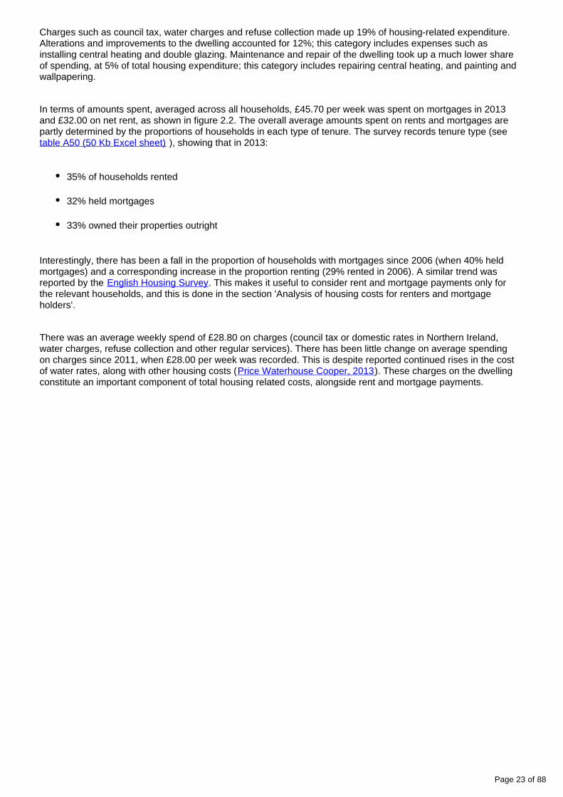
Figure 2.1: Housing expenditure items as a percentage of total housing expenditure, 2013

United Kingdom


This section considers the breakdown of housing expenditure, averaged across all households, regardless of whether or not they hold a mortgage or pay rent.

As shown in figure 2.1, mortgage payments accounted for 31% of housing expenditure in 2013; this includes interest payments, protection premiums and capital repayments. Net rent accounts for 22% of housing expenditure; this refers to the rent payments that the householders have to meet themselves, so benefits and rebates received by the household to help pay for rent have been subtracted.

http://www.ons.gov.uk/ons/rel/family-spending/family-spending/2014-edition/rft-2-2-final-2013.xls

http://www.ons.gov.uk/ons/rel/family-spending/family-spending/2014-edition/art-appendix-a.html


Page 23 of 88

Charges such as council tax, water charges and refuse collection made up 19% of housing-related expenditure. Alterations and improvements to the dwelling accounted for 12%; this category includes expenses such as installing central heating and double glazing. Maintenance and repair of the dwelling took up a much lower share of spending, at 5% of total housing expenditure; this category includes repairing central heating, and painting and wallpapering.

In terms of amounts spent, averaged across all households, £45.70 per week was spent on mortgages in 2013 and £32.00 on net rent, as shown in figure 2.2. The overall average amounts spent on rents and mortgages are partly determined by the proportions of households in each type of tenure. The survey records tenure type (see

), showing that in 2013:table A50 (50 Kb Excel sheet)

35% of households rented

32% held mortgages

33% owned their properties outright

Interestingly, there has been a fall in the proportion of households with mortgages since 2006 (when 40% held mortgages) and a corresponding increase in the proportion renting (29% rented in 2006). A similar trend was reported by the . This makes it useful to consider rent and mortgage payments only for English Housing Surveythe relevant households, and this is done in the section 'Analysis of housing costs for renters and mortgage holders'.

There was an average weekly spend of £28.80 on charges (council tax or domestic rates in Northern Ireland, water charges, refuse collection and other regular services). There has been little change on average spending on charges since 2011, when £28.00 per week was recorded. This is despite reported continued rises in the cost of water rates, along with other housing costs ( ). These charges on the dwelling Price Waterhouse Cooper, 2013constitute an important component of total housing related costs, alongside rent and mortgage payments.


https://www.gov.uk/government/uploads/system/uploads/attachment_data/file/284648/English_Housing_Survey_Headline_Report_2012-13.pdf

http://www.pwc.co.uk/the-economy/publications/uk-economic-outlook/ukeo-summary-july13.jhtml

Page 24 of 88

Figure 2.2: Housing expenditure 2011 to 2013


Spending on alterations and improvements was £17.70 in 2013, compared with £19.60 in 2011 (without adjusting for inflation). Interestingly, there has recently been official encouragement for homeowners to improve their properties, such as one run by the and the government revamped . Home Improvement Agency Green DealThese schemes focus on ensuring existing housing is fit for purpose for elderly, disabled or low income home owners, by assisting financially in making homes more energy efficient or providing lists of reliable builders for any work required. This might be a factor in the absence of increased expenditure in this category in recent years.

6 . Analysis of housing costs for renters and mortgage holders

The following section looks at average expenditure on net rent for households that report spending on rent and expenditure on mortgages for mortgage holders. This is the only place in this report where averages are not calculated across all households. This is because including only households that do pay rent or hold a mortgage provides a more informative picture of expenditure on these important elements of household expenditure.

http://www.foundations.uk.com/about-home-improvement-agencies/

https://www.gov.uk/green-deal-energy-saving-measures

Page 25 of 88

Expenditure on net rent increased slightly in 2013 ( ). On average renters spent table 2.8 (35.5 Kb Excel sheet)£92.10 per week in 2013; this is an increase from 2012 (£86.40) and 2011 (£77.00) without adjusting for inflation. These findings are consistent with other sources such as the where it was found that the English Housing Surveyaverage weekly rents in both the private and social rented sectors increased in 2012-13. The Index of Private

also found that between May 2012 and May 2013 private rental prices grew by 1.3% in Housing Rental PricesGreat Britain.

Expenditure on mortgages rose in 2013, without adjusting for inflation. The average weekly expenditure on mortgages by mortgage holders was £145.40 in 2013, compared with £138.60 in 2012 ( table 2.9 (34.5 Kb Excel

). Analysis of rent in this publication tends to focus on net rent, because this is what is used in calculations sheet)of total expenditure. Average spending on gross rent by renting households (£138.40 per week) is very similar to spending on mortgages by mortgage holders. Gross rent refers to the rent payable in total, including the elements that are met by benefits and rebates, rather than householders.

Figure 2.3 and show mortgage payments by mortgage holders and net rent table 2.10 (74 Kb Excel sheet)payments by renters broken down by income band. The first income decile comprises the tenth of households with the lowest income, the second decile the tenth of households with the next highest incomes, and so on. The figures should be treated with caution, because there are low numbers of renters, or mortgage holders in the survey sample for some income groups: relatively few low-income households hold mortgages and high income households rent.

Figure 2.3: Expenditure on net rent by renters, and mortgages by mortgage holders, by gross income decile group, 2013

United Kingdom


http://www.ons.gov.uk/ons/rel/family-spending/family-spending/2014-edition/rft-table-2-8-final-2013.xls


http://www.ons.gov.uk/ons/dcp171766_311546.pdf

http://www.ons.gov.uk/ons/dcp171766_311546.pdf




Page 26 of 88

As might be expected, spending both on mortgages (by mortgage holding households) and net rent (by rent paying households) increased as income increased. Among the lowest-income households, average spending on net rent (£31.70 per week) was much lower than mortgage payments (£74.20 per week). Among higher income groups the pattern was different, with spending on net rent higher than mortgage payments. For the tenth of households with the highest incomes, net rent expenditure averaged £268.60 and mortgage payments £233.20 per week. This pattern is largely due to housing benefits and rebates, which make renting markedly less expensive for lower-income households, but have almost no impact on higher earning households. Average weekly expenditure on gross rent was £118.10 for the lowest-income ten per cent of households, much higher than the £31.70 net rent figure.

7 . Housing expenditure by socio-demographic characteristics

The relationship between income and housing expenditure was reflected in associated socio-demographic characteristics, such as socio-economic classification of the Household Reference Person (HRP, defined in

), as shown in . Where the HRP was in an occupation defined as being appendix B table 2.6 (78 Kb Excel sheet)“higher managerial or large employer”, housing expenditure averaged £299.20 per week; this was much higher than £104.50 per week if the HRP was in a routine occupation.

Age is another important factor. Housing expenditure is presented in by the age table 2.4 (60 Kb Excel sheet)group of the HRP. Households where the HRP was aged between 30 and 49 spent the most on housing (£199.40 per week). Higher spending in this age group is driven largely by mortgage payments, which were £84.10 per week compared with £45.70 for all age groups combined. This is the age range where households tend to take up mortgages, and take the greatest responsibility for meeting the payments. By contrast, younger households, where the HRP was aged under 30, spent an average of £88.40 on net rent, much higher than the overall figure of £32.00. It’s not surprising that households with younger HRPs tend to spend more on rent, as many people in this age group have not yet acquired the means or stability of lifestyle to maintain a mortgage.

8 . Expenditure by region/country

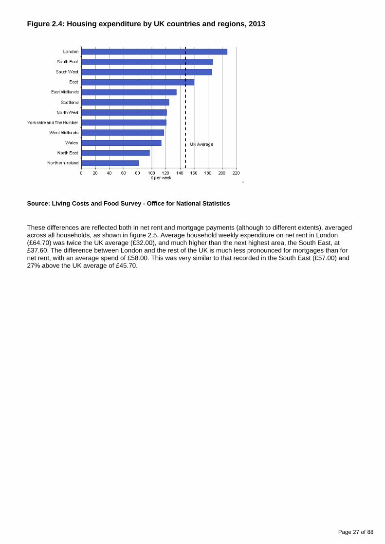
There are large variations in average expenditure on housing across different regions of the UK, as shown in figure 2.4 and . The pattern is very similar to that recorded for total expenditure. table 2.5 (54.5 Kb Excel sheet)The UK average household weekly expenditure on housing was £147.90 in 2013. London households spent the most at £206.90 per week; followed by the South East (£186.30) and the South West (£184.80). The lowest spending areas were Northern Ireland (£81.00) and the North East (£96.50). This is largely reflected in the average house price across different regions of the UK. The showed house prices ONS House Price Index (HPI)were most expensive in London in 2013 with an average of £424,000, followed by the South East (£300,000), whereas the UK average house price was £242,000; Northern Ireland was the least expensive region with an average of £130,000. The prices given are “mix-adjusted” prices, as explained in the HPI bulletin.





http://www.ons.gov.uk/ons/rel/hpi/house-price-index/september-2014/index.html

Page 27 of 88

Figure 2.4: Housing expenditure by UK countries and regions, 2013


These differences are reflected both in net rent and mortgage payments (although to different extents), averaged across all households, as shown in figure 2.5. Average household weekly expenditure on net rent in London (£64.70) was twice the UK average (£32.00), and much higher than the next highest area, the South East, at £37.60. The difference between London and the rest of the UK is much less pronounced for mortgages than for net rent, with an average spend of £58.00. This was very similar to that recorded in the South East (£57.00) and 27% above the UK average of £45.70.

http://www.ons.gov.uk/ons/resources/figure24final2013_tcm77-386373.png

Page 28 of 88

Figure 2.5: Percentage difference compared with UK average for mortgage payments and net rent payments by UK countries and regions, 2013

United Kingdom


A slightly different pattern emerges when considering only rent payers and mortgage holders, by region, as shown in . For net rent, London is less far ahead of other areas (£141.60, table 2.11 (70.5 Kb Excel sheet)compared with the UK average of £92.10) than when rent figures are averaged across all households. This reflects the fact that higher average expenditure on rent in London is partly driven by the high proportion of renters in the capital. established that London accounted for the largest percentage of 2011 Census analysisrenters at 50.4% of households. The other factor is rental prices, which are higher in London than other parts of the UK, as found by an [Index of Housing Rental Prices (IHRP) report].

For mortgages, higher spending by London’s households can be seen more clearly when looking at expenditure by mortgage holders only. The capital’s spending averaged £211.80 per week; the next highest areas were the South East (£172.10) and the East (£158.90). The confirmed that London has a lower proportion of 2011 Censusmortgage holding households than many other areas with just 27.1% of owner occupiers compared to the UK average of 32.7%, pushing down the spending averaged across all households. However, property prices are high in London ( ) and its mortgage holding households paid considerably more The ONS House Price Index, HPIthan in other parts of the UK.


http://www.ons.gov.uk/ons/rel/census/2011-census-analysis/a-century-of-home-ownership-and-renting-in-england-and-wales/index.html

http://www.ons.gov.uk/ons/rel/census/2011-census-analysis/a-century-of-home-ownership-and-renting-in-england-and-wales/index.html

http://www.ons.gov.uk/ons/rel/hpi/house-price-index/september-2014/index.html

Page 29 of 88

1.

2.

3.

4.

5.

6.

7.

8.

9.

10.

11.

12.

Expenditure on housing reflects both the characteristics of the geographic area of the household and of the household itself. There are complex interactions between these factors as house prices and rental costs are influenced by the demands of the local population and the perceived desirability of an area of residence. There are large differences in housing-related expenditure among regions of the UK, with London standing out as the area with the highest expenditure both on rent and mortgages.

9 . Definitions of housing expenditure

The COICOP system has been used to classify expenditure on the Living Costs and Food Survey (LCF) and previously the Expenditure and Food Survey (EFS) since 2001/02.

COICOP is an internationally agreed system of classification for reporting consumption expenditure within National Accounts and is used by other household budget surveys across the European Union.

Further information on COICOP can be found on the .United Nations Statistics Division website

Under COICOP, household consumption expenditure is categorised into the following 12 headings:

Food and non-alcoholic drinks

Alcoholic drinks, tobacco and narcotics

Clothing and footwear

Housing (net), fuel and power

Household goods and services

Health

Transport

Communication

Recreation and culture

Education

Restaurants and hotels

Miscellaneous goods and services

It is important to note that COICOP classified housing costs do not include what is considered to be non-consumption expenditure, for example: mortgage interest payments, mortgage capital repayments, mortgage protection premiums, council tax and domestic rates.

In addition to the 12 COICOP expenditure categories, the tables contained in appendix A include a category called ‘other expenditure items’ under which certain non-consumption expenditures can be found. This category includes the following housing-related costs: mortgage interest payments, mortgage protection premiums, council tax, and domestic rates. Housing costs that are not included in the COICOP definition of housing or the ‘other expenditure items’ category are captured within the ‘other items recorded’ category that can be viewed in table

in appendix A.A1 (153.5 Kb Excel sheet)

http://unstats.un.org/unsd/cr/registry/regct.asp?Lg=1



Page 30 of 88

For the purpose of this chapter all data relating to housing expenditure have been combined to facilitate an understanding of total housing costs. This comprehensive definition of housing expenditure is made up from three types of expenditure detailed in table 2.1: expenditure included in COICOP, housing costs in the ‘other expenditure items’ and ‘other items recorded’ categories of this report.

Page 31 of 88

2.1: Definition of total housing expenditure

Costs which are included in the COICOP classification of housing expenditure:

Actual rentals for housing

– net rent (gross rent less housing benefit, rebates and allowances received)

– second dwelling rent

Maintenance and repair of dwelling

– central heating maintenance and repair

– house maintenance and repair

– paint, wallpaper, timber

– equipment hire, small materials

Water supply and miscellaneous services relating to dwelling

– water charges

– other regular housing payments including service charge for rent

– refuse collection, including skip hire.

Housing costs which are included elsewhere in the COICOP classification:

Household Insurances

– structural insurance

– contents insurance

– insurance for household appliances.

Housing costs which are included as ‘other expenditure items’ but excluded from COICOP classification:

Housing: mortgage interest payments etc.

– mortgage interest payments

– mortgage protection premiums

– council tax, domestic rates

– council tax, mortgage, insurance (second dwelling).

Housing costs which are included as ‘other items recorded’ and are excluded from COICOP classification:

Purchase or alteration of dwellings (contracted out), mortgages

– outright purchase of houses, flats etc. including deposits

– capital repayment of mortgage

– central heating installation

– DIY improvements: double glazing, kitchen units, sheds etc.

– home improvements (contracted out)

– bathroom fittings

– purchase of materials for capital improvements

– purchase of second dwelling.


Page 32 of 88

1.

2.

3.

4.

5.









Contacts






Media enquiries


Editor




About us









Page 33 of 88




5.

6.





Tel: +44 (0)20 8876 3444


ISSN 2040-1647


gsi.gov.uk


Compendium

Chapter 3: Equivalised incomeA report on the Living Costs and Food Survey 2013, including spending on housing, utilities and other outgoings.

Table of contents

1. Abstract

2. Key points

3. Background

4. Income, expenditure and well-being

5. Household expenditure by income

6. Household expenditure by household composition and income

7. Equivalisation methodology

8. Equivalisation results





Page 34 of 88

9. Background notes

Page 35 of 88

1 . Abstract

This chapter examines how expenditure varies with equivalised income. Equivalised income is household income that has been recalculated to take into account the fact that households with many members are likely to need a higher income to achieve the same standard of living as households with fewer members.

2 . Key points

Lower income households spend a higher proportion of their total expenditure on food and drink than higher income households (16% compared to 8%), although households in the highest income group spent £35 more per week than households in the lowest income group

The proportion of total expenditure on recreation and culture increased with income (9% to 15%). This reflects the expectation that higher income households have more income available to spend on discretionary items

Expenditure patterns differ between retired and non-retired households. For example, among one person households spending on clothing and footwear increased by £21.60 for non-retired households between the top and bottom income groups, compared to an increase of £2.40 for retired households

Spending on food and drink by income differed for one person households, in comparison to the overall pattern for all household types. There was little variation in spending by one person households as income increased (£10.20 for one person non-retired households, £6.00 for one person retired households, compared to £34.70 for all households)

3 . Background

This chapter examines how expenditure varies with equivalised income, which refers to household income that has been recalculated to take into account differences in household size and composition.

Equivalisation is a standard methodology that adjusts household income to account for the different financial resource requirements of different household types. Household size is an important factor to consider because larger households usually need a higher income than smaller households to achieve a comparable standard of living. The composition of a household also affects resource needs, for example, living costs for adults are normally higher than for children. After equivalisation has been applied, households with the same equivalised income can be said to have a comparable standard of living.

Data for disposable income has been published and is reported on in this chapter. Gross income tables are available on request. Disposable income is defined as gross weekly cash income less the statutory deductions and payments of income tax and National Insurance contributions . Most analysis looking at income and 1

expenditure together looks at disposable rather than gross income. This is because disposable income is the amount that households have available to spend or save.

Full details of the equivalisation methodology used are given in the 'Equivalisation Methodology' section. Information on how the equivalisation process affects the distribution of income data for different household types is in the 'Equivalisation Results' section.

Notes for background

Page 36 of 88

1. For other ONS and DWP publications, council tax and domestic rates (Northern Ireland) are also deducted from gross income to provide a measure of disposable income. For Family Spending council tax and domestic rates (Northern Ireland) are counted as expenditure within the total expenditure definition.

4 . Income, expenditure and well-being

For many households, income is their most important economic resource for meeting everyday living expenses. However, it is the consumption of goods and services (best reflected by expenditure) that is pivotal in meeting a household's requirements. As highlighted in the remainder of this section evidence suggests that income and expenditure together represent a better determinant of economic well-being than income alone.

Expenditures change less than incomes when short term changes in incomes are encountered, and can therefore be considered a better proxy of living standards. Households can smooth expenditure by, for example, adjusting savings, drawing on wealth and borrowing, whereas incomes may be more volatile. This led to Friedman’s ‘permanent income hypothesis’, which suggests that decisions made by consumers are based on long-term income expectations rather than their current income. describe expenditure Headey, Muffels and Wooden, 2004as ‘the most valid measure of current living standards’ in their analysis of household finances and well-being.

In addition, recent ONS analysis shows that household spending matters more to many aspects of personal well-being than household income. As spending rises, average life satisfaction (the sense that what one does in life is worthwhile) and happiness also rise ( ).Lewis, 2014

The Commission on the Measurement of Economic Performance and Social Progress ( Stiglitz, Sen and Fitoussi, ) recommended that greater prominence should be given to the distributions of income and expenditure 2009

across households.

For given levels of expenditure, and everything else being equal, people with higher income can be seen as having a higher level of well-being from a personal finance perspective than people with lower income. With higher income, they have greater opportunity to increase expenditure if they want, or to save income to finance expenditure in the future.

In light of this context, this chapter examines how expenditure varies with income.

5 . Household expenditure by income

This section illustrates how separating the expenditure patterns for different types of goods and services provides a fuller picture of how households with different levels of income spend their money.

Tables 3.1 (422 Kb Excel sheet) and show expenditure, in total and for each of the 3.1E (89 Kb Excel sheet)Classification of Individual COnsumption by Purpose (COICOP) categories, by non-equivalised and equivalised disposable income decile groups respectively.

As shown in figure 3.1, there was an overall increase in total expenditure as equivalised income, and non-equivalised income increased. In 2012 there was a similar pattern, although the second equivalised income decile had a slightly lower expenditure than the bottom non-equivalised income decile. This is often referred to as an ‘expenditure tick’.

http://ftp.iza.org/dp1218.pdf

http://www.ons.gov.uk/ons/rel/wellbeing/measuring-national-well-being/income--expenditure-and-personal-well-being/art--income--expenditure-and-personal-well-being.html

http://www.stiglitz-sen-fitoussi.fr/documents/rapport_anglais.pdf

http://www.stiglitz-sen-fitoussi.fr/documents/rapport_anglais.pdf


http://www.ons.gov.uk/ons/rel/family-spending/family-spending/2014-edition/rft-3-1e-final-2013.xls

Page 37 of 88

Figure 3.1: Household expenditure by non-equivalised and OECD-modified equivalised disposable income decile group, 2013

United Kingdom


In 2012 it was suggested that an ‘expenditure tick’ could be partly due to consumption smoothing. Consumption smoothing is caused by individuals who have a low income on a short-term basis but who have higher expenditure than expected for their level of income, such as students and the temporarily unemployed. The absence of the expenditure tick in 2013 could be due to the fall in the unemployment rate between 2012 and 2013 as reported in . The number of unemployed adults who were Labour Market Statistics, February 2014expecting to start work within the next few weeks fell, potentially reducing the impact of the temporarily unemployed whose spending may have been based on expected future income. However, as the Living Costs and Food Survey only collects information on households’ current income sources, it is not possible to establish whether longer term income expectations account for the expenditure pattern observed.

Expenditure in the lower income decile groups increased after income was equivalised. This is due to the impact the equivalisation method has on the income positioning of households with children, and single adult households. Equivalisation increases the number of households with children in the lower income groups, whose spending is likely to be higher than households containing one adult. These households tend to move to a higher income decile group after income is equivalised. For more details see 'Equivalisation Results'.

Tables 3.2 (481 Kb Excel sheet) and show the share of total expenditure on table 3.2E (118.5 Kb Excel sheet)each COICOP category, by non-equivalised and equivalised income groups. The rest of this section compares the absolute spending and the share of total expenditure by equivalised disposable income for different categories of spending.

http://www.ons.gov.uk/ons/rel/lms/labour-market-statistics/february-2014/statistical-bulletin.html


http://www.ons.gov.uk/ons/rel/family-spending/family-spending/2014-edition/rft-3-2e-final-2013.xls

Page 38 of 88

Expenditure on food and non-alcoholic drink rose with equivalised income, whilst the proportion of total expenditure on food and non-alcoholic drink decreased (see figure 3.2). Clearly all households have to spend a certain amount on food and non-alcoholic drink. However, as income rises households spend more in absolute terms on this category, but there is a limit to how much food households consume and the amount they are willing to spend overall. As a result of this, households in the higher equivalised disposable income decile groups spend a lower proportion of their expenditure on food and non-alcoholic drink than households in the lower income decile groups. As income rises from the lowest to the highest equivalised disposable income decile group, spending almost doubles from £40.70 to £75.40. However, for households in the bottom equivalised disposable income decile group food and non-alcoholic drinks accounted for 16% of total expenditure, compared to 8% for the top equivalised disposable income decile group.

Figure 3.2: Expenditure on food and non-alcoholic drinks (absolute expenditure and as a percentage of total expenditure) by OECD-modified equivalised disposable income decile group, 2013

United Kingdom


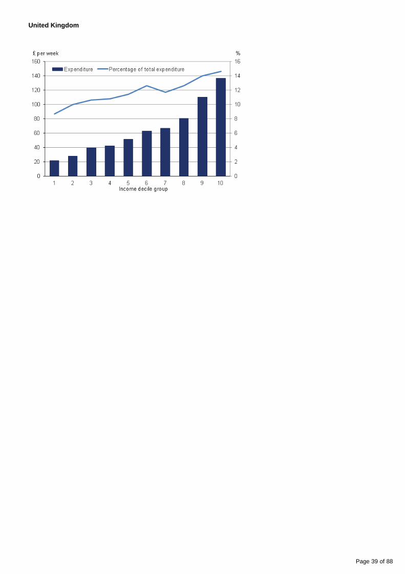
For certain categories where spending can be seen as non-essential, the proportion of total expenditure increased, as well as the amount. An example of this is recreation and culture, which includes expenditures that are almost entirely non-essential (such as package holidays, sports admissions and audio-visual equipment). Higher income households may be expected to have more available to spend on recreational activities, for example, package holidays abroad where the pattern is particularly evident. Figure 3.3 shows the highest equivalised income households spent £137 per week on recreation and culture. This is around six times as much as households in the lowest equivalised income decile, which only spent £22 per week. The proportion of spending increases from 9% to 15%. Figure 3.4 shows a breakdown of selected lower-level items in recreation and culture, showing the pattern above for package holidays.

Figure 3.3: Expenditure on recreation and culture (absolute expenditure and as a percentage of total expenditure) by OECD-modified equivalised disposable income decile group, 2013

Page 39 of 88

United Kingdom

Page 40 of 88


Figure 3.4: Expenditure on recreation and culture and selected lower-level items by OECD-modified equivalised disposable income decile group, 2013

United Kingdom


6 . Household expenditure by household composition and income

This section looks at how expenditure varies with income for retired and non-retired households containing one adult (see tables 3.3 to 3.10 and tables 3.3E to 3.10E). One adult retired and non-retired households have been chosen as an example of how expenditure varies with income for different household types. Retired households are those where the householder has reached state pension age, is not working or seeking work, and is mainly dependent on income sources other than the state pension (for example, occupational pension, income from investments, or annuities). Retired households mainly dependent on state pensions have been excluded from this analysis as they have low sample sizes.

Page 41 of 88

As seen in figure 3.5, total expenditure for both non-retired and retired households containing one adult rose with equivalised disposable income quintile (these increased by £375 per week for non-retired households, and £308 per week for retired households). For each quintile group, absolute spending was higher for households containing one non-retired adult. Most individual expenditure categories showed a similar pattern, but for some categories the variation in spending with income was more or less marked.

Figure 3.5: Expenditure for one adult households by OECD-modified equivalised disposable income quintile group, 2013

United Kingdom


Spending on food and non-alcoholic drink was similar for both types of household for the second to fifth income quintiles, as shown in figure 3.6. There is much less variation in spending between income quintile groups for both household types as compared to the overall picture of expenditure on food and non-alcoholic drink seen in figure 3.2, where there is a strong trend of expenditure increasing with income. This suggests spending additional income on food is less of a priority for one-person households than for other household types.

Page 42 of 88

Figure 3.6: Expenditure on food and non-alcoholic drinks for one adult households by OECD-modified equivalised disposable income quintile group, 2013

United Kingdom


For non-retired households made up of one adult, spending on clothing and footwear increased sharply as equivalised disposable income increased. However, there was very little increase among retired households. Spending on essential clothing is expected for all households but clothing offers a broad range of price. The pattern seen for one adult non-retired households may be due to higher income households choosing to buy more expensive items, or choosing to buy more new clothes. The contrasting pattern seen in one person retired higher income households may reflect a lower priority for buying expensive or new clothes compared to other categories of spending.

Page 43 of 88

Figure 3.7: Expenditure on clothing and footwear for one adult households by OECD-modified equivalised disposable income quintile group, 2013

United Kingdom


Households containing one retired and non-retired adult have broadly similar levels and patterns of spending on household goods and services. Higher-earning retired and non-retired households spend more on items such as furniture, household appliances, and household garden tools. Non-retired households only spend notably more on these (arguably non-essential) expenditure items in the highest income quintile than retired households.

Page 44 of 88

Figure 3.8: Expenditure on household goods and services for one adult households by OECD-modified equivalised income quintile group, 2013

United Kingdom


As figure 3.9 shows, there is a general pattern of increasing expenditure on restaurants and hotels for both one adult non-retired and retired households, with non-retired households consistently spending more over income bands.

Page 45 of 88

Figure 3.9: Expenditure on restaurants and hotels for one adult households by OECD-modified equivalised disposable income quintile group, 2013

United Kingdom


These points illustrate how expenditure requirements differ between retired and non-retired households; note that non-retired households tend to have higher incomes. Income quintiles have been calculated separately for retired and non-retired households for this analysis, so patterns of expenditure within these groups can be explored meaningfully.

Examining spending patterns by income allows us to see how households prioritise spending on essentials, and how they balance this with enjoying some non-essential goods and services. The analysis above suggests that retired and non-retired households prioritise spending additional income differently for some spending categories. Equivalisation is a powerful tool to understand how income relates to the needs and choices of households of different sizes and compositions. The complex findings give some clues as to what is important for well-being.

looks at how spending patterns have changed over time.Chapter 4

7 . Equivalisation methodology

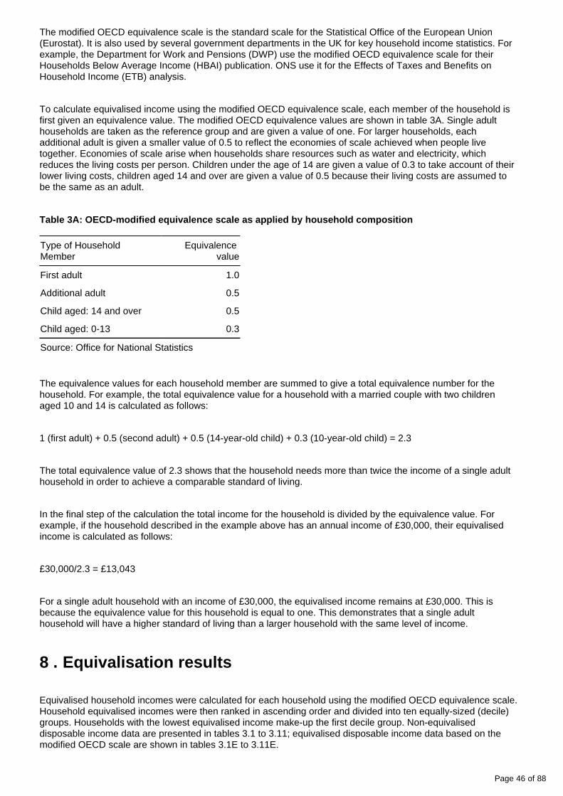
Equivalisation scales are used to adjust household income, taking into account household size and composition. There are various scales available, which differ in their complexity and methodology. The so-called OECD modified equivalence scale is used widely across Europe. It adjusts household income to reflect the different resource needs of single adults, any additional adults in the household, and children in various age groups.


Page 46 of 88

The modified OECD equivalence scale is the standard scale for the Statistical Office of the European Union (Eurostat). It is also used by several government departments in the UK for key household income statistics. For example, the Department for Work and Pensions (DWP) use the modified OECD equivalence scale for their Households Below Average Income (HBAI) publication. ONS use it for the Effects of Taxes and Benefits on Household Income (ETB) analysis.

To calculate equivalised income using the modified OECD equivalence scale, each member of the household is first given an equivalence value. The modified OECD equivalence values are shown in table 3A. Single adult households are taken as the reference group and are given a value of one. For larger households, each additional adult is given a smaller value of 0.5 to reflect the economies of scale achieved when people live together. Economies of scale arise when households share resources such as water and electricity, which reduces the living costs per person. Children under the age of 14 are given a value of 0.3 to take account of their lower living costs, children aged 14 and over are given a value of 0.5 because their living costs are assumed to be the same as an adult.

Table 3A: OECD-modified equivalence scale as applied by household composition

Type of Household Member

Equivalence value

First adult 1.0

Additional adult 0.5

Child aged: 14 and over 0.5

Child aged: 0-13 0.3


The equivalence values for each household member are summed to give a total equivalence number for the household. For example, the total equivalence value for a household with a married couple with two children aged 10 and 14 is calculated as follows:

1 (first adult) + 0.5 (second adult) + 0.5 (14-year-old child) + 0.3 (10-year-old child) = 2.3

The total equivalence value of 2.3 shows that the household needs more than twice the income of a single adult household in order to achieve a comparable standard of living.

In the final step of the calculation the total income for the household is divided by the equivalence value. For example, if the household described in the example above has an annual income of £30,000, their equivalised income is calculated as follows:

£30,000/2.3 = £13,043

For a single adult household with an income of £30,000, the equivalised income remains at £30,000. This is because the equivalence value for this household is equal to one. This demonstrates that a single adult household will have a higher standard of living than a larger household with the same level of income.

8 . Equivalisation results

Equivalised household incomes were calculated for each household using the modified OECD equivalence scale. Household equivalised incomes were then ranked in ascending order and divided into ten equally-sized (decile) groups. Households with the lowest equivalised income make-up the first decile group. Non-equivalised disposable income data are presented in tables 3.1 to 3.11; equivalised disposable income data based on the modified OECD scale are shown in tables 3.1E to 3.11E.

Page 47 of 88

The income decile groups can be seen in table 3B.

Table 3B: Income deciles for disposable weekly income and disposable weekly equivalised income, 2013

Income decile Disposable weekly income

Disposable weekly equivalised income (OECD-modified scale)

1 Up to £173 Up to £141

2 £174 to £255 £142 to £188

3 £256 to £332 £189 to £230

4 £333 to £416 £231 to £277

5 £417 to £503 £278 to £318

6 £504 to £599 £319 to £368

7 £600 to £719 £369 to £431

8 £720 to £881 £432 to £519

9 £882 to £1149 £520 to £663

10 £1,150 and over £664 and over


Table 3.12 (43.5 Kb Excel sheet) shows the household composition of the non-equivalised disposable income decile groups and the OECD-equivalised disposable income decile groups. Equivalisation has a large impact on the income positioning of households containing one adult without children. Households containing one non-retired adult accounted for only 3% of households in the highest non-equivalised disposable income decile group but when income was equivalised they accounted for 16%. These households tended to move to a higher income decile group after income was equivalised. These results demonstrate that when equivalisation is used to look at the incomes of all households on a comparable basis, single adult households tend to be better off than they appear pre-equivalisation.

The percentage of households where the household reference person is retired in each income group, before and after equivalisation is shown in figure 3.10. Equivalisation has a large effect on the proportion of retired households in the lowest income decile group. Before equivalisation, 15% of all retired households appeared in the lowest non-equivalised disposable income decile group; after equivalisation, only 7% of retired households appeared in this group. This result can largely be explained by the fact that a relatively high proportion of retired households contain only one adult. Therefore, as explained above, the incomes of single adult households are scaled up (relative to other households) when income is equivalised. The proportion of retired households in the second and third lowest income deciles also decreased after equivalisation, although the effect was much smaller. The opposite was true of the higher income decile groups; the proportion of retired households increased slightly after income was equivalised.


Page 48 of 88

Figure 3.10: Percentage of retired households by non-equivalised and OECD-modified equivalised income decile group, 2013

United Kingdom


Figure 3.11 shows the percentage of households with children in each income group, before and after income equivalisation. As non-equivalised disposable income increases, the proportion of households with children generally increases through the lower and middle income groups. Factoring in living costs for children as part of the equivalisation process brings about large changes in the income distribution. There are more households with children in the lower income groups and there is no longer an increase in the number of households with children as income increases.

Page 49 of 88

Figure 3.11: Percentage of households with children in each non-equivalised and OECD-modified equivalised income decile group, 2013

United Kingdom


Table 3.12 (43.5 Kb Excel sheet) also shows how equivalisation affects the average household size for each income decile group. As non-equivalised disposable income increases the average number of people in each household also increases. The average household size for the highest income group (3.2 people) was almost two and a half times that of the lowest income group (1.3 people). After income was equivalised, the average number of people in each household was more similar for each income decile group, with the average varying between 2.1 and 2.5. This pattern of results occurs because the equivalisation process scales up the income of households containing one adult (relative to other households) and scales down the income of households with more people.

This is the only chapter that presents equivalised income data. Other tables included in Family Spending are available on an equivalised income basis on request from ONS (see ‘About this edition of Family Spending’).


Page 50 of 88

1.

2.

3.

4.

5.

9. Background notes








Contacts






Media enquiries


Editor




About us









Page 51 of 88




5.

6.





Tel: +44 (0)20 8876 3444


ISSN 2040-1647


gsi.gov.uk


Compendium

Chapter 4: Trends in household expenditure over timeA report on the Living Costs and Food Survey 2013, including spending on housing, utilities and other outgoings.

Table of contents

1. Abstract

2. Key points

3. About this chapter

4. Trends in average household spending

5. Trends in spending patterns

6. Background

7. Background notes





Page 52 of 88

1 . Abstract

This chapter examines trends in household expenditure over time. Table 4.1 and table 4.2 (see tables section) represent expenditure for the years 2001/02 to 2013, adjusted to take account of inflation mainly using the Consumer Prices Index (CPI). This enables a comparison of expenditure to be made between survey years that allows for changing prices. More detail on this is given in the Background section. Year-on-year comparisons must be treated with caution, because each year the LCF is reviewed and changes are made to keep it up to date. Expenditure over the same period is also shown without adjusting for inflation in table 4.3 (see tables section).

2 . Key points

Household average weekly expenditure has decreased since 2006, once inflation has been taken into account

Spending declined to £517.30 in 2013, from its peak in 2006 (adjusted to 2013 prices) when households spent an average of £539.80 per week

Between 2001/2 and 2006, average expenditure was at a higher level than that seen since 2006

Housing (net), fuel and power accounted for the highest average weekly spending in 2013, at £74.40, an increase from £70.70 in 2012 (adjusted to 2013 prices). Renting was the biggest area of expenditure in this category, followed by electricity gas and other fuels (it does not include mortgage payments, council tax or Northern Ireland rates). This category accounted for 14% of household expenditure, on average, in 2013

Transport remains the second highest expenditure category, averaging £70.40 per week in 2013. This was an increase from £64.80 per week in 2012, driven by an increase in the sales of new cars. However, transport expenditure has decreased in recent years from £88.00 in 2001/2 (adjusted for inflation)

The results show slight increases across a range of expenditure categories. However, these findings should be treated with caution due to changes to the way the survey recorded certain types of expenditure in 2013

3 . About this chapter

This chapter examines trends in household expenditure over time. and Table 4.1 (82.5 Kb Excel sheet) table 4.2 present expenditure for the years 2001/2 to 2013, adjusted to take account of inflation (91.5 Kb Excel sheet)

using mainly the Consumer Prices Index (CPI). This enables a comparison of expenditure to be made between survey years that allows for changing prices. Expenditure over the same period is also shown without adjusting for inflation ( ).table 4.3 (82 Kb Excel sheet)

Changes and differences mentioned in the text have been found to be statistically significant at the 95% confidence level, unless stated. There is more detail in the background section.

4 . Trends in average household spending

This section discusses some of the trends seen in average household weekly spending since 2001/2, once the effects of inflation have been taken into account.





Page 53 of 88

1.

2.

3.

Figure 4.1: Total household expenditure based on COICOP classification, 2001-02 to 2013, at 2013 prices [1]

United Kingdom


Notes:




Figure 4.1 shows total expenditure over the years from 2001/2 to 2013. The figures have been adjusted to 2013 prices, to allow for the effects of inflation. Average weekly household spending was £539.80 in 2006, and started declining, just before the economic downturn, in 2007 (when £531.70 per week was recorded). Average spending decreased further to £501.00 in 2012, and then increased to £517.30 in 2013 . 1 Table 4.1 (82.5 Kb Excel sheet)shows that household income declined slightly later than expenditure, following the start of the downturn. Disposable household income peaked in 2008 at £676 (adjusted to 2013 prices), declining to £612 in 2012 and £614 in 2013 .2


Page 54 of 88

1.

2.

The trend observed in household spending after 2008 is broadly consistent with the wider economic context. Between 2008 quarter 1 and 2009 quarter 2, Gross Domestic Product (GDP) fell by 6.0%, marking the deepest economic downturn since ONS records began in 1948. The latest downturn is similar to the 5.9% fall in the early 1980s, while output fell by 2.4% in the early 1990s. The subsequent recovery has also been the . slowestHowever, the UK economy showed signs of increasing momentum throughout 2013 with GDP growing by 1.7%. The UK economy is now estimated to have surpassed the quarter 1 2008 pre-downturn peak in the quarter 3 2013. These figures can be found on the .Office for National Statistics website

If spending is considered without adjusting for inflation we see a different trend. Household spending, at the prices at the time the surveys were carried out, has increased from £398.30 in 2001/2 to £517.30 in 2013.

Notes for trends in average household spending

This increase was not found to be significant at the 95% confidence level; refer to the background section of the chapter for further details.

Standard errors are not calculated for income estimates in Family Spending. Therefore this change has not been tested for statistical significance at the 95% confidence level; refer to the background section of the chapter for further details.

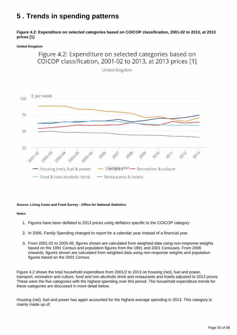
http://www.ons.gov.uk/ons/rel/elmr/economic-review/september-2014/art-er-sept.html

http://www.ons.gov.uk/ons/rel/naa2/quarterly-national-accounts/q2-2014/stb-quarterly-national-accounts--q2-2014.html

Page 55 of 88

1.

2.

3.

5 . Trends in spending patterns

Figure 4.2: Expenditure on selected categories based on COICOP classification, 2001-02 to 2013, at 2013 prices [1]

United Kingdom


Notes:




Figure 4.2 shows the total household expenditure from 2001/2 to 2013 on housing (net), fuel and power, transport, recreation and culture, food and non-alcoholic drink and restaurants and hotels adjusted to 2013 prices. These were the five categories with the highest spending over this period. The household expenditure trends for these categories are discussed in more detail below.

Housing (net), fuel and power has again accounted for the highest average spending in 2013. This category is mainly made up of:

Page 56 of 88

net rent: £32.00 per week in 2013

electricity gas and other fuels: £26.50 in 2013

maintenance and repair of dwelling: £7.10 in 2013

water supply and miscellaneous charges: £8.70 in 2013.

Note: these figures are averaged across all households, for example, whether they pay rent or not.

The category housing (net), fuel and power does not include mortgage payments. Mortgage interest payments are included within the “other expenditure items” category. Spending in this category has fluctuated over time, decreasing overall from £78.30 in 2001/2 (adjusted for inflation) to £73.00 in 2013 ( 1 table 4.1 (82.5 Kb Excel

). Capital repayment of mortgages for 2013 is detailed in section 14 (“other items recorded”) of sheet) table A1 of this report. A full picture of housing related expenditure is provided in Chapter 2, (153.5 Kb Excel sheet)

including those, such as mortgage payments, that fall outside the Classification of Individual COnsumption by Purpose (COICOP) classification.

Rent payments make up the largest proportion of household expenditure in the category housing (net), fuel and power. The number of households renting accommodation has increased over recent years, as reported by the

. This is supported by figures published in of Family English Housing Survey table A50 (50 Kb Excel sheet)Spending for 2013, and the corresponding table for 2006, which showed the proportion of households renting increased, from 29% in 2006 to 35% in 2013 . Therefore, the increased proportion of households renting has 2

contributed to higher spending on housing (net), fuel and power.

Average household spending on transport decreased between 2001/2 (adjusted to 2013 prices) and 2013. However, it increased to £70.40 in 2013, from £64.80 per week in 2012. Households allocated an average of 14% of total expenditure to transport in 2013. Higher average household expenditure on transport between 2012 and 2013 can partly be attributed to increased purchase of new cars. Vehicle purchases were recorded as being at a six-year high with 1,074,622 new private .cars registered

Purchasing new cars is an area where households could moderate or defer expenditure, which may lead to demand building up over time. This is sometimes referred to as “pent up demand”. This may have fuelled the increase in sales of new cars seen in 2013, with consumers replacing vehicles they kept hold of through the recent downturn.

Recent years have seen the price of petrol and diesel increase substantially, with costs rising above the overall rate of inflation in 2012. However, between 2012 and 2013 prices so the increase in transport decreased slightlyexpenditure in 2013 cannot be attributed to spending on fuel.

Decreases in expenditure have been seen in categories that include some elements of discretionary spending, but not all. For example, spending on restaurants and hotels has gradually decreased to £40.40 in 2013, from £48.50 in 2001/2. This suggests that, in less favourable economic conditions, households are prepared to limit their spending on hotel stays and restaurant visits.

In contrast, overall spending on recreation and culture increased between 2001/2 and 2013, from £53.80 (adjusted for inflation) to £63.90 on average per week. This category includes a wide range of expenditure, including: information processing equipment, games, gardening items, sport, cinema and theatre admissions, and package holidays. A common feature of these products and services is that they would generally be considered to constitute discretionary spending (though see discussion below), so it is interesting that these types of expenditures have held up over time. For example, package holidays abroad accounted for an average of £21.00 per week of household expenditure in 2013 . This reflects the continued growth of the UK cruise market, with the 3

continuing to grow by 1.5% in 2013. Expenditure on items such as TV, number of people taking an ocean cruisevideo, computers and recreational activities has also held up over time, showing the high priority placed on these goods and services by many households, regardless of economic circumstances.







http://www.smmt.co.uk/2014/01/2013-new-car-market-records-best-performance-five-years

https://www.gov.uk/government/statistical-data-sets/oil-and-petroleum-products-monthly-statistics

http://www.cruiseexperts.org/media/700262/ocean_cruise_figures_2013.pdf

Page 57 of 88

1.

2.

3.

There has been a slight decrease in the average weekly expenditure on alcoholic drinks, tobacco and narcotics in 2013 compared with 2012. Average weekly expenditure has gone down from £18.20 in 2001/2 to £12.00 in 2013, once inflation has been taken into account. Another likely factor is the well-documented decrease in the proportion of people who smoke; show that the proportion of people smoking has latest smoking figuresdecreased to 19% in 2013, from 27% in 2000.

Expenditure on clothing and footwear has fluctuated only slightly over the years 2011 to 2013 (when a weekly average of £22.60 was recorded). This is following a substantial increase from £15.40 in 2001/2 (adjusted for inflation). Spending on food and non-alcoholic drink remained very similar for the years 2011 to 2013 (£58.80 in 2013), having fallen from £65.00 in 2006.

The trend in expenditure after 2008 is broadly consistent with the wider economic context. There has been an overall reduction in weekly spending from 2001/2 to 2013 in real terms, but a slight (not-statistically significant) increase between 2012 and 2013. GDP is estimated to have increased by 1.7% in 2013, compared with 2012, showing signs of the economic recovery building momentum.

The trends for different types of spending show that consumers may be remaining price conscious following the economic downturn. For example, consumers are continuing to spend less on certain items that may be considered discretionary such as restaurants and hotels, and alcohol and tobacco. The picture is not straightforward, however, as decreases have not been observed over time on clothing and footwear, and goods and services in the recreation and culture category. This highlights that the label “discretionary” should be treated with caution since items or services that may have traditionally been considered discretionary, may be considered essential by many households after they get used to having these products. By contrast, other goods, such as tobacco, may become considered less desirable over time.

The economy has witnessed signs of economic recovery, despite consumers remaining price conscious. There is evidence that consumer confidence is increasing slowly; increases in household expenditure are largely focused on items such as housing. However, the results have also seen an increase in expenditure on big ticket items, such as new cars in 2013, indicating that pent up demand is being realised.

The year-on-year changes presented in this chapter should be treated with caution because changes in recording expenditure were implemented by the Living Costs and Food (LCF) survey in 2013.

Notes for trends in spending patterns

This increase was not found to be significant at the 95% confidence level; refer to the background section of the chapter for further details

Standard errors are not calculated for table A50 of the Family Spending report 2013. Therefore this change has not been tested for statistical significance at the 95% confidence level; refer to the background section of the chapter for further details.

Recording of spending on package holidays was also subject to questionnaire changes in 2013.

6 . Background

This chapter presents household expenditure data over time using the Classification of Individual COnsumption by Purpose (COICOP) classification. The expenditure figures have been deflated to allow comparison of expenditure in real terms across survey years.

http://www.ons.gov.uk/ons/rel/ghs/opinions-and-lifestyle-survey/adult-smoking-habits-in-great-britain--2013/index.html

Page 58 of 88

1.

2.

The figures and tables present figures that have been deflated to 2013 prices using the consumer prices index (CPI), using indices specific to each major COICOP category. This is with the exception of specific items to which the CPI is not applicable: for mortgage interest payment and council tax payments the Retail Prices Index (RPI) was used. The approach used to deflate figures to 2013 prices is consistent with the approach used for Family Spending, 2012. However, it is different from editions previous to this, when the all-items RPI was used.

Tables based on the Family Expenditure Survey (FES) classification, used by the survey for years prior to 2001/2, have been reported in previous editions. They are not presented here, but can be made available on request. The time series presented, based on COICOP, has been increased to include 2001/2 to 2013; the range of years on which the survey has reported on COICOP.

The LCF is reviewed every year and changes are made to keep it up to date. Therefore, year-on-year changes should be interpreted with caution. This is particularly relevant for 2013 data; substantial changes were made to the questionnaire following research and testing. These changes included recording of household utility expenses, purchase of furniture and spending on air fares. It is important to continue to review the survey, to make sure it captures all types of spending as fully as possible, in an environment where products and methods of payment change rapidly. A detailed breakdown of the items that feed into each COICOP heading can be found in .table A1 (153.5 Kb Excel sheet)

Standard errors for categories with lower levels of spending tend to be higher, so trends for these categories need to be treated with a degree of caution. Standard errors have been calculated for the data presented in this chapter; including the figures that have been deflated to 2013 prices (standard errors are discussed in more detail in ). These calculations have been taken into account in the testing for statistical significance. This appendix Btesting indicates the probability with which we are confident that the difference between the estimates under examination did not occur by chance.

Changes and differences mentioned have been found to be statistically significant at the 95% confidence level, unless stated. This means that the probability that the difference occurred by chance is low (1 in 20 or lower). Note that spending on certain items, notably tobacco and alcohol, may be under-reported.

COICOP time series data in this publication are not directly comparable with UK National Accounts household expenditure data, published in Consumer Trends (this publication can be downloaded from the Office for National

). National Accounts figures draw on a number of sources in addition to the LCF (Statistics website Consumer has more details) and may be more appropriate for finding long term trends on expenditure.Trends guidance

7. Background notes












http://www.ons.gov.uk/ons/guide-method/method-quality/specific/economy/consumer-trends/index.html

http://www.ons.gov.uk/ons/guide-method/method-quality/specific/economy/consumer-trends/index.html

Page 59 of 88

2.

3.

4.

5.

6.

Contacts






Media enquiries


Editor




About us









Tel: +44 (0)20 8876 3444


ISSN 2040-1647






Page 60 of 88

Next release: 8 December 2015



6. Details of the policy governing the release of new data are available by visiting www.statisticsauthority.gov. or from the Media Relations Office email: uk/assessment/code-of-practice/index.html media.relations@ons.

gsi.gov.uk


Compendium

Survey methodology: Appendix BAppendix B provides further detailed information regarding the methodology of the Living Costs and Food survey, used to produce the estimates presented in Family Spending.

Table of contents

1. Description of the survey

2. Uses of the survey

3. Response to the survey

4. Weighting

5. Standard errors and estimates of precision

6. Survey improvements

7. Comparison with another source

8. Definitions

9. Headings used for identifying 2013 income information

10. Household characteristics and index to tables





Page 61 of 88

1 . Description of the survey

A household expenditure survey has been conducted each year in the UK since 1957. From 1957 to March 2001 the Family Expenditure Survey (FES) and National Food Survey (NFS) provided information on household expenditure patterns and food consumption. In April 2001 these surveys were combined to form the Expenditure and Food Survey (EFS).

In 2008 selected Government household surveys, on which the Office for National Statistics (ONS) leads, were combined into one Integrated Household Survey (IHS). In anticipation of this, the EFS moved to a calendar-year basis in January 2006. The EFS questionnaire became known as the Living Costs and Food (LCF) module of the IHS in 2008, to accommodate the insertion of a core set of IHS questions.

More information about the IHS can be found on the ONS website. In summary, the survey design allows for the collection of common core data across the pooled samples of the constituent surveys, achieving the biggest pool of UK social data after the Census. The large sample allows a detailed level of analysis to be conducted, and allows results to be reported for smaller geographic areas. The IHS has become the key vehicle for high-profile national data collection initiatives including questions on subjective well-being, and on sexual identity.

The LCF is a voluntary sample survey of private households. The basic unit of the survey is the household. A household comprises one person living alone or a group of people (not necessarily related living at the same address) who share cooking facilities AND share a living room or sitting room or dining area (See ‘Definitions’).

Each individual aged 16 and over in the household visited is asked to keep diary records of daily expenditure for two weeks. Information about regular expenditure, such as rent and mortgage payments, is obtained from a household interview along with retrospective information on certain large, infrequent expenditures such as those on vehicles. Children aged 7 to 15 are asked to keep a simplified version of the diary.

Detailed questions are asked about the income of each adult member of the household. In addition, personal information such as age, sex and marital status is recorded for each household member. A copy of the LCF questionnaire is available from the .UK Data Service

The survey is continuous, interviews being spread evenly over the year to ensure that seasonal effects are covered. The questionnaire content is reviewed thoroughly to ensure that it is up-to-date and captures information efficiently. Some changes reflect new forms of expenditure or new sources of income, especially benefits. Others are the result of new requirements by the survey’s users. (See the section on ‘Survey Improvements’ for more information.)

The sample design

The LCF sample for Great Britain is a multi-stage stratified random sample with clustering. It is drawn from the Small Users file of the Postcode Address File (PAF) – the Post Office’s list of addresses. All Scottish offshore islands and the Isles of Scilly are excluded from the sample because of excessive interview travel costs. Postal sectors are the primary sample unit. 638 postal sectors are randomly selected after being arranged in strata defined by Regions (sub-divided into metropolitan and non-metropolitan areas) and two 2001 Census variables: socio-economic group of the head of household and ownership of cars. These census variables were new stratifiers originally introduced for the 1996/97 survey, and updated following the results of the 2001 Census. The results of the 2011 Census will be used in due course. The Northern Ireland sample is drawn as a random sample of addresses from the Land and Property Services Agency list.

2 . Uses of the survey

http://discover.ukdataservice.ac.uk/series/?sn=2000028

Page 62 of 88

LCF expenditure data

Retail Prices Index – The main reason, historically, for instituting a regular survey on expenditure by households has been to provide information on spending patterns for the Retail Prices Index (RPI) and the Consumer Prices Index (CPI). From April 2011 the CPI rather than the RPI is used as basis for indexation of benefits, tax credit and state and public service pensions. The RPI and CPI measure the change in the cost of a selection of goods and services (the ‘basket of goods’) representative of the expenditure of the vast majority of households. The pattern of expenditure gradually changes from one year to the next, and the composition of the basket of goods needs to be kept up-to-date. Accordingly, regular information is required on spending patterns and much of this is supplied by the LCF. The expenditure weights for the general RPI and CPI need to relate to people within given income limits, for which the LCF is the only source of information.

Household expenditure and Gross Domestic Product (GDP) – LCF data on spending are an important source used in compiling national estimates of household final consumption expenditure which are published regularly in United Kingdom National Accounts (ONS Blue Book). Household final consumption expenditure estimates feed into the National Accounts and estimates of GDP. They will also provide the weights for Purchasing Power Parities (PPPs) for international price comparisons. LCF data are also used in the estimation of taxes on expenditure, in particular VAT.

Regional accounts – LCF expenditure information is one of the sources used by ONS to derive regional estimates of consumption expenditure. It is also used in compiling some of the other estimates for the regional accounts.

The statistical office of the European Union (Eurostat) collates information from family budget surveys conducted by the member states. The LCF is the UK’s contribution to this important EU initiative to collect data on household expenditure from member countries.

Other government uses – The Department of Energy and Climate Change and the Department for Transport both use LCF expenditure data in their own fields relating to, for example, energy, housing, cars and transport. The Department for Transport uses LCF data to monitor and forecast levels of car ownership and use, and in studies on the effects of motoring taxes.

Non-government uses – There are also numerous users outside central government, including academic researchers and business and market researchers. One example is an academic study that has used LCF data, as part of a wider study, to obtain a clear picture of utility expenditure patterns across the European Union.

LCF income data

Redistribution of income – LCF information on income and expenditure is used to study how government taxes and benefits affect household income. The Government’s interdepartmental tax benefit model is based on the LCF and enables the economic effects of policy measures to be analysed across households. This model is used by HM Treasury and HM Revenue and Customs to estimate the impact on different households of possible changes in taxes and benefits.

Non-government users – As with the expenditure data, LCF income data are also studied extensively outside government. In particular, academic researchers in the economic and social science areas of many universities use the LCF. For example the Institute for Fiscal Studies uses LCF data in research it carries out both for government and on its own account to inform public debate.

Family Spending and Defra reporting

The Department for Environment, Food and Rural Affairs (Defra) publishes separate reports using LCF data on food expenditure to estimate consumption and nutrient intake.

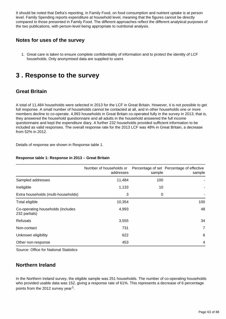
Page 63 of 88

1.

It should be noted that Defra's reporting, in Family Food, on food consumption and nutrient uptake is at person level. Family Spending reports expenditure at household level, meaning that the figures cannot be directly compared to those presented in Family Food. The different approaches reflect the different analytical purposes of the two publications, with person-level being appropriate to nutritional analysis.

Notes for uses of the survey

Great care is taken to ensure complete confidentiality of information and to protect the identity of LCF households. Only anonymised data are supplied to users

3 . Response to the survey

Great Britain

A total of 11,484 households were selected in 2013 for the LCF in Great Britain. However, it is not possible to get full response. A small number of households cannot be contacted at all, and in other households one or more members decline to co-operate. 4,993 households in Great Britain co-operated fully in the survey in 2013; that is, they answered the household questionnaire and all adults in the household answered the full income questionnaire and kept the expenditure diary. A further 232 households provided sufficient information to be included as valid responses. The overall response rate for the 2013 LCF was 48% in Great Britain, a decrease from 52% in 2012.

Details of response are shown in Response table 1.

Response table 1: Response in 2013 – Great Britain

Number of households or addresses

Percentage of set sample

Percentage of effective sample

Sampled addresses 11,484 100 -

Ineligible 1,133 10 -

Extra households (multi-households) 3 0 -

Total eligible 10,354 100

Co-operating households (includes 232 partials)

4,993 48

Refusals 3,555 34

Non-contact 731 7

Unknown eligibility 622 6

Other non-response 453 4


Northern Ireland

In the Northern Ireland survey, the eligible sample was 251 households. The number of co-operating households who provided usable data was 152, giving a response rate of 61%. This represents a decrease of 6 percentage points from the 2012 survey year .1

Page 64 of 88

Northern Ireland was over-sampled in the years 1997/98 to 2009 in order to provide a large enough sample for some separate analysis. This boost to the Northern Ireland sample was discontinued in 2010.

Partial response

Three types of partial response are accepted on the LCF:

All adults complete the full income section of the interview, but one or more adults in the household refuse to keep the diary

All adults in the household keep the diary, but one or more adults provides only partial income information

One or more adults refuse to keep the diary and one or more adults provide only partial income information

All partial responses must contain a diary from the Main Diary Keeper (MDK), who is the person who does most of the shopping in the household. If the MDK refuses to complete the diary the household is classified as a refusal.

In 2013 partial responses accounted for 5% (232 households) of all co-operating households. Of these partials, the majority (97%) occurred because one or more adults in the household refused to keep the diary. Partial income information was provided in 3% of cases.

Response table 2: Type of partial response in 2013 – Great Britain

Type of partial response Number of households

Percentage of partials

1. One or more adults refuse to keep the diary 1 225 97

2. One or more adults provide only partial income information

7 3

All 232 100


Notes:

1. Diary is present for the main diary keeper.

LCF Response rates over time

Response rates to household surveys have generally been declining in recent years. In 2013 the LCF’s response rate for Great Britain was 48% (see ‘Response to the survey’ for a detailed breakdown), compared with around 59% in 2000/01. Response in 2013 was lower than in 2012, when 52% was achieved. It should be noted that the LCF requires satisfactory completion of both the household questionnaire and diary. For more information see the ‘ '.Living Costs and Food Survey Technical Report (529.7 Kb Pdf)

http://www.ons.gov.uk/ons/guide-method/method-quality/specific/social-and-welfare-methodology/living-costs-and-food-survey/living-costs-and-food-survey-technical-report-for-survey-year-january-december-2013.pdf

Page 65 of 88

The Fieldwork

The fieldwork is conducted by the Office for National Statistics (ONS) in Great Britain and by the Northern Ireland Statistics and Research Agency (NISRA) of the Department of Finance and Personnel in Northern Ireland using almost identical questionnaires. Households at the selected addresses are visited and asked to co-operate in the survey. In order to maximise response, interviewers make at least four separate calls, and sometimes many more, at different times of day on households which are difficult to contact. Interviews are conducted by Computer Assisted Personal Interviewing (CAPI) using laptop computers.

During the interview information is collected about the household; certain regular payments such as rent, gas, electricity and telephone accounts; expenditure on certain large items (for example vehicle purchases over the previous 12 months); and income. Each individual aged 16 and over in the household is asked to keep a detailed record of expenditure every day for two weeks.

Children aged between 7 and 15 are also asked to keep a simplified diary of daily expenditure. In 2013 a total of 1,318 children aged between 7 and 15 in responding households in the UK were asked to complete expenditure diaries; 249, or 19%, did not do so. This number includes both refusals and children who had no expenditure during the two weeks. Information provided by all members of the household is kept strictly confidential. Each person aged 16 and over in the household who keeps a diary (and whose income information is collected) is subsequently sent a £10 voucher as a token of appreciation. Children who keep a diary are given a £5 voucher.

Some survey cases are reissued if a response is not obtained, that is, the cases are reallocated to field interviewers at a later date to attempt to achieve a response. In 2013 859 addresses were reissued, of which 25 were converted into responding households. This increased the overall response by 0.2 percentage points.

Eligible response

Under LCF rules, a refusal by just one person to respond to the income section of the questionnaire invalidates the response of the whole household. Similarly, a refusal by the household’s main shopper to complete the two-week expenditure diary also results in an invalid response.

Proxy response

Questions about general household affairs are put to all household members or to the household representative person (HRP), and questions about work and income are put to the individual members of the household. Where a member of the household is not present during the household interview, another member of the household (for example a spouse) may be able to provide information about the absent person. The individual’s interview is then identified as a proxy interview. Under LCF rules, the expenditure diary cannot be completed by proxy; if a household member is not present during the diary period they are classified as an absent spender.

In 2013 the percentage of fully responding households with a proxy interview in Great Britain was 26%. Analysis of the 2013 data revealed that the inclusion of proxy interviews increased response from above average income households. For the 2013 survey, the average gross normal weekly household income was 21% higher than it would have been if proxy interviews had not been accepted.

Similar findings were obtained with respect to expenditure: total spending was 15% higher than if proxy interviews had not been included. Use of proxies enhances the sample size and hence the precision of the figures obtained. It also enables the survey to capture the income and expenditure from (on average) higher-earning households and hence ensures that these households are represented fully in the survey. This must be weighed against the risk that the proxy interviews may not provide exactly the same information as direct interviews, but the available evidence suggests that including proxies provides higher data quality overall.

Page 66 of 88

1.

Reliability

Great care is taken in collecting information from households, and comprehensive checks are applied during processing so that errors in recording and processing are minimised. The main factors that affect the reliability of the survey results are sampling variability, non-response bias and some incorrect reporting of certain items of expenditure and income. Measures of sampling variability are given alongside some results in this report and are discussed in detail in ‘Standard errors and estimates of precision’.

The households which decline to respond to the survey tend to differ in some respects from those that co-operate; it is therefore possible that their patterns of expenditure and income also differ. Currently, non responders are accounted for in the weighting process for LCF data, which compensates for non responders recognised from analysis of the 2001 Census (see ‘Weighting’ for more information). At present, the LCF is contributing towards the 2011 Census non-response linkage project, which will enable non-response weights to be updated.

Checks are included in the computer assisted personal interviewing (CAPI) program, which are applied to the responses given during the interview. Other procedures are also in place to ensure that users are provided with high quality data. For example, quality control is carried out to ensure that any unusual values (outliers) are genuine, and checks are made on any unusual changes in average spending compared with the previous year.

Income and expenditure balancing

The LCF is designed primarily as a survey of household expenditure on goods and services. It also gathers information about the income of household members, and is an important and detailed source of income data. However, it is not possible to draw up a balance sheet of income and expenditure either for individual households or groups of households.

The majority of expenditure information collected relates to the two-week period immediately following the interview, whereas income components can refer to a much longer period (the most recent 12 months). LCF income does not include withdrawal of savings; loans and money received in payment of loans; receipts from maturing insurance policies; proceeds from the sale of assets (such as a car); and winnings from betting or windfalls, such as legacies. Despite this, recorded expenditure might reflect these items, as well as the effects of living off savings, using capital, borrowing money or income – either recent or from a previous period.

Hence, there is no reason why income and expenditure should balance. In fact measured expenditure exceeds measured income at the bottom end of the income distribution. However, this difference cannot be regarded as a reliable measure of savings or dis-saving.

For further information of what is included in income on the LCF see ‘Income headings’.

Imputation of missing information

Although LCF response is generally based on complete households responding, there are areas in the survey for which missing information is imputed (inferred, sometimes in conjunction with other sources). This falls into two broad categories: item imputation and diary imputation. Using a combination of reliable imputation procedures ensures that the LCF data provide a comprehensive picture of the spending patterns and income sources for each household. For more information see the ‘ '.Living Costs and Food Survey Technical Report (529.7 Kb Pdf)

Notes for response to the survey

In 2012, the eligible Northern Ireland sample was 256 households. The number of co-operating households who provided usable data was 171 households, giving a response rate of 67%.


Page 67 of 88

4 . Weighting

Since 1998/99 the survey has been weighted to reduce the effect of non-response bias and produce population totals and means. The weights are produced in two stages. First, the data are weighted to compensate for non-response (sample-based weighting). Second, the sample distribution is weighted so that it matches the population distribution in terms of region, age group and sex (population-based weighting).

Sample based weighting using the Census

Weighting for non-response involves giving each respondent a weight so that they represent the non-respondents that are similar to them in terms of the survey characteristics. Non responders are accounted for in the weighting process for LCF data using results from the 2001 Census linked study of non responders.

The 2001 LCF Census-linked study matched census addresses with the sampled addresses of EFS. In this way it was possible to match the address details of the respondents as well as the non-respondents with corresponding information gathered from the Census for the same address. The information collected during 2001 Census/EFS matching work was then used to identify the types of households that were being under-represented in the survey. Further details of how the weighting classes were produced can be seen in the ‘Weighting’ section of the ‘

'.Living Costs and Food Survey Technical Report (529.7 Kb Pdf)

The results of the 2011 Census-linked studies will be used to further update non-response weighting in due course.

Population-based weighting

The second stage of the weighting adjusts the non-response weights so that weighted totals match population totals. As the LCF sample is based on private households, the population totals used in the weighting need to relate to people living in private households. For 2013 data the population totals used were population projections based on estimates rolled forward from the 2011 Census, adjusted to harmonise with the LCF definition of a private household. These estimates used exclude residents of institutions not covered by the LCF, such as those living in bed-and-breakfast accommodation, hostels, residential homes and other institutions.

The non-response weights were calibrated1 so that weighted totals matched population totals for males and females in different age groups and for regions. An important feature of the population-based weighting is that it is done by adjusting the factors for households not individuals.

The weighting is carried out separately for each quarter of the survey. The main reason is that sample sizes vary more from quarter to quarter than in the past. This is due to reissuing addresses after an interval of a few months where there had previously been no contact or a refusal to a new interviewer. This results in more interviews in the later quarters of the year than in the first quarter. Quarterly weighting, therefore, counteracts any potential bias from the uneven spread of interviews through the year. Quarterly weighting also results in small sample numbers in some of the age/sex categories that were used in previous years. The categories have therefore been widened slightly to avoid this.

Effects of weighting on the data

Table B1 shows the effects of the weighting by comparing unweighted and weighted data from 2013.


Page 68 of 88

1.

Table B1: The effect of weighting on expenditure, 2013

United Kingdom

Commodity or service Average weekly household expenditure (£)

Absolute difference

Percentage difference

Unweighted Weighted as published

All expenditure groups 441.50 444.30 2.79 0.6

Food and non-alcoholic drinks 59.30 58.80 -0.53 -0.9

Alcoholic drink, tobacco & narcotics

12.10 12.00 -0.10 -0.8

Clothing and footwear 22.40 22.60 0.18 0.8

Housing, fuel and power 70.00 74.40 4.36 6.2

Household goods and services 33.80 33.10 -0.68 -2.0

Health 6.60 6.20 -0.39 -5.8

Transport 70.80 70.40 -0.31 -0.4

Communication 14.20 14.50 0.27 1.9

Recreation and culture 66.40 63.90 -2.46 -3.7

Education 6.80 8.80 1.96 28.6

Restaurants and hotels 39.80 40.40 0.59 1.5

Miscellaneous 39.20 39.10 -0.10 -0.2

Weekly household income:

Disposable 608 614 7 1.1

Gross 727 739 12 1.6


The weighting decreased the estimate of total average expenditure by £2.79 a week. It had the largest impact on average weekly expenditure on education, increasing the estimate by 28.6%. It also increased the estimate of spending on housing, fuel and power by 6.2%, and reduced the estimate of spending on recreation and culture by 3.7% and the estimate for household goods and services by 2.0%. Weighting also increased the estimates of average income, by £7 a week for disposable household income and by £12 a week (1.6%) for gross household income, which is the income used in most tables in the report.

Re-weighting also has an effect on the variance of estimates. In an analysis on the 1999/2000 data, weighting increased variance slightly for some items and reduced it for others. Overall the effect was to reduce variance slightly.

Notes for weighting

Implemented by the CALMAR software package before 2007 and GES for 2006–08 (updated weights).

Page 69 of 88

5 . Standard errors and estimates of precision

The Living Costs and Food Survey (LCF) is a sample of households and not a census of the whole population. Therefore, the results are liable to differ to some degree from those that would have been obtained if every single household had been covered. Some of the differences will be systematic, in that lower proportions of certain types of household respond than of others. That aspect is discussed in ‘Response to the survey’ and ‘Weighting’. This section discusses the effect of sampling variability; in other words, the effect of differences in expenditure and income between the households in the sample and in the whole population that arise from random chance.

The degree of variability will depend on the sample size and how widely particular categories of expenditure (or income) vary between households. The sampling variability is smallest for the average expenditure of large groups of households on items purchased frequently and when the level of spending does not vary greatly between households. Conversely, it is largest for small groups of households, and for items purchased infrequently or for which expenditure varies considerably between households. A numerical measure of the likely magnitude of such differences (between the sample estimate and the value of the entire population) is provided by the quantity known as the standard error.

The calculation of standard errors takes into account the fact that the LCF sample is drawn in two stages: first a sample of areas (primary sampling units), then a sample of addresses within each of these areas. The main features of the sample design are described in ‘Description of the survey’. The calculation also takes account of the effect of weighting. The two-stage sample increases sampling variability slightly, but the weighting reduces it for some items.

Standard errors for detailed expenditure items are presented in relative terms in table A1 (153.5 Kb Excel sheet)(standard error as a percentage of the average to which it refers). As the calculation of full standard errors is complex, this is the only table where they are shown. Tables B2 and B3 in this section show the design factor (DEFT), a measure of the efficiency of the survey’s sample design. The DEFT is calculated by dividing the full standard error by the standard error that would have applied if the survey had used a simple random sample.

Further standard errors are calculated for the figures and tables in the trends chapter. Figures have been deflated to 2013 prices using the Consumer Prices Index (CPI), using indices specific to each major COICOP category. This is with the exception of specific items to which the CPI is not applicable: for mortgage interest payment and council tax payments the Retail Prices Index (RPI) was used. For the deflated figures using the CPI, standard errors have been calculated. For more information of the calculation of standard errors see the ‘ Living Costs and

'.Food Survey Technical Report (529.7 Kb Pdf)




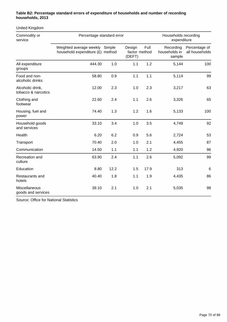
Page 70 of 88

Table B2: Percentage standard errors of expenditure of households and number of recording households, 2013

United Kingdom

Commodity or service

Percentage standard error Households recording expenditure

Weighted average weekly household expenditure (£)

Simple method

Design factor

(DEFT)

Full method

Recording households in

sample

Percentage of all households

All expenditure groups

444.30 1.0 1.1 1.2 5,144 100

Food and non-alcoholic drinks

58.80 0.9 1.1 1.1 5,114 99


12.00 2.3 1.0 2.3 3,217 63

Clothing and footwear

22.60 2.4 1.1 2.6 3,326 65

Housing, fuel and power

74.40 1.3 1.2 1.6 5,133 100

Household goods and services

33.10 3.4 1.0 3.5 4,749 92

Health 6.20 6.2 0.9 5.6 2,724 53

Transport 70.40 2.0 1.0 2.1 4,455 87

Communication 14.50 1.1 1.1 1.2 4,920 96

Recreation and culture

63.90 2.4 1.1 2.6 5,092 99

Education 8.80 12.2 1.5 17.9 313 6

Restaurants and hotels

40.40 1.8 1.1 1.9 4,435 86

Miscellaneous goods and services

39.10 2.1 1.0 2.1 5,035 98


Page 71 of 88

Table B3: Percentage standard errors of income of households and number of recording households, 2013

United Kingdom

Source of income Percentage standard error Households recording income

Weighted average weekly household expenditure (£)

Simple method

Design factor

(DEFT)

Full method

Recording households in

sample

Percentage of all

households

Gross household income 739.00 1.3 1.1 1.3 5,130 100

Wages and salaries 481.00 1.9 1.0 1.9 2,980 58

Self-employment 54.00 6.4 0.9 5.9 648 13

Investments 25.00 8.0 1.1 8.7 2,325 45

Annuities and pensions (other than social security benefits)

67.00 3.7 0.8 3.0 1,770 35

Social security benefits 102.00 1.6 0.7 1.1 3,684 72

Other sources 9.00 7.7 1.1 8.4 638 12


Using the standard errors – calculating confidence intervals

A common use of standard errors is in calculating confidence intervals. Confidence intervals can be used to estimate a range within which the true population value should lie in. The 95% interval can be taken to mean that there is only a 5% chance that the true population value lies outside the 95% confidence interval (or that 95 times out of 100 the true population value will fall within the interval).

The following formulae are used to calculate a 95% confidence interval:

Lower limit: mean - 1.96 × (percentage standard error ÷ 100) × mean

Upper limit: mean + 1.96 × (percentage standard error ÷ 100) × mean

For example, using the expenditure on food and non-alcoholic drinks to illustrate this calculation; the average expenditure is £58.80 and the corresponding percentage standard error (full method) is 1.1% (rounded to one decimal place). The limits for a 95% confidence interval are then:

Lower limit: 58.80 - 1.96 × (1.1 ÷ 100) ×58.80 = £57.60

Upper limit: 58.80 + 1.96 × (1.1 ÷ 100) ×58.80 = £60.00

Similar calculations can be carried out for other estimates of expenditure and income. The 95% confidence intervals for main expenditure categories are given in table B4.

Page 72 of 88

Table B4: 95 per cent confidence intervals for average household expenditure, 2013

United Kingdom

Commodity or service Weighted average weekly household expenditure (£)

95% confidence interval

Lower limit Upper limit

All expenditure groups 444.30 434.00 454.60

Food and non-alcoholic drinks 58.80 57.60 60.00


12.00 11.50 12.60

Clothing and footwear 22.60 21.50 23.70

Housing, fuel and power 74.40 72.10 76.70

Household goods and services 33.10 30.90 35.40

Health 6.20 5.50 6.90

Transport 70.40 67.50 73.30

Communication 14.50 14.10 14.80

Recreation and culture 63.90 60.70 67.20

Education 8.80 5.70 11.90

Restaurants and hotels 40.40 38.80 41.90

Miscellaneous goods and services 39.10 37.50 40.80


Using the standard errors – statistical significance testing

Statistical significance testing indicates the probability with which we are confident that the difference between the estimates under examination did not occur by chance. Significance testing carried out in the trends chapter is at the 95% level unless otherwise stated. This means the probability that the difference happened by chance is low (1 in 20). For more information of the method used for significance testing see the ‘ Living Costs and Food

'.Survey Technical Report (529.7 Kb Pdf)

6 . Survey improvements

Questionnaire review

In order to ensure the LCF questionnaire is up-to-date it is important that questions are regularly reviewed so that relevant changes can be made. Reviewing the questionnaire is a process of continuous improvement. For example, a pilot survey was carried out in 2012 to evaluate further questionnaire improvements. The changes tested in the pilot have been implemented for the 2013 survey year. Questionnaire changes included: the addition of a new breakdown of spending on different types of furniture and package holidays; collection of flight expenditure in the questionnaire rather than the diary; the addition of a section designed to capture expenditure on combined utility packages; and the addition of new questions about mobile phone ownership.



Page 73 of 88

7 . Comparison with another source

A useful comparison for LCF estimates is with Household Final Consumption Expenditure (HHFCE) figures published in and used in the UK National Accounts.Consumer Trends

This section compares estimates from the LCF with the estimates used in the UK National Accounts. The Household Final Consumption Expenditure estimates use a number of administrative and survey sources, of which the LCF survey is one. As a result differences occur in the estimates published, because of sources and concepts.

For example, conceptual differences can be found for housing expenditure. As explained in Chapter 2: Housing , Family Spending only includes rental costs in the housing, fuel and power category, whilst mortgage expenditure

costs are included in the other expenditure items category. In contrast, National Accounts housing data in the housing, fuel and power category includes a value for rentals paid by owner occupiers in order to maintain international comparability. This is a theoretical cost that home owners would have to pay to rent their own home. By international convention, mortgage costs are excluded from National Accounts Household Final Consumption Data.

According to Family Spending data, housing, water, electricity, gas and other fuels was the category where the value of spending increased most over the period 2006 to 2013 (without adjusting for inflation, an increase of 36%). Despite the conceptual differences between the two outputs, National Accounts household expenditure estimates for the same category also show a large increase (54%) in spending.

Both National Accounts and of Family Spending provide estimates over time to remove the effects of Chapter 4inflation and to enable figures for different years to be compared on a like-for-like basis. The National Accounts figures adjusted for inflation are known as "volume measures". The volume measures of National Accounts show that housing expenditure has increased 7%, while the prices of goods and services in this category, measured as an implied deflator, have increased by 44% between 2006 and 2013. Adjusted for inflation, Family Spending shows an increase in housing expenditure of 12% over the same period (from £65.40 to £74.40).

A similar pattern can be seen in the food and non-alcoholic drinks category in National Accounts data, showing a reduction in volume (3%) and an increase in the monetary value of spending by around 35% since 2006. Family Spending reported a 21% increase in spending on food since 2006 (from £46.30 to 58.80, not adjusted for inflation). These figures indicate relatively little scope or willingness to cut back on these items, despite significant price rises in some goods and services and the recession of 2008/2009.

Family Spending shows that transport spending at 2013 prices fell from £80.50 in 2006 to £70.40 in 2013, a decrease of 14%. The National Accounts household expenditure on transport shows that spending adjusted for inflation fell by 2%. Prices in this category, again measured as an implied deflator, increased by 40% over the period which suggests that, as with food and non-alcoholic beverages, the rise in prices influenced households’ decisions to reduce their purchases.

8 . Definitions

Household

A household comprises of one person living alone or a group of people (not necessarily related) living at the same address who:

share cooking facilities

and share a living room or sitting room or dining area

http://www.ons.gov.uk/ons/publications/all-releases.html?definition=tcm%3A77-23619




Page 74 of 88

Resident domestic servants are included. The members of a household are not necessarily related by blood or marriage. As the survey covers only private households, people living in hostels, hotels, boarding houses or institutions are excluded. Households are included if some or all members are not British subjects, however, information is not collected from households containing members of the diplomatic service of another country or members of the United States armed forces.

Retired households

Retired households are those where the household reference person is retired. The household reference person is defined as retired if they have reached state pension age and are economically inactive. Since May 2010 the state pension age for women has been increasing gradually to be in line with the male pension age of 65 by 2018. Therefore, if for example a male household reference person is aged over 65 years of age, but working part-time or waiting to take up a part-time job, this household would not be classified as a retired household. For analysis purposes two categories are used in this report:

‘A retired household mainly dependent upon state pensions’ is one in which at least three-quarters of the total income of the household is derived from national insurance retirement and similar pensions, including housing and other benefits paid in supplement to or instead of such pensions. The term ‘national insurance retirement and similar pensions’ includes national insurance disablement and war disability pensions, and income support in conjunction with these disability payments.

‘Other retired households’ are retired households which do not fulfil the income conditions of 'retired household mainly dependent upon state pensions’ because more than a quarter of the households income derives from other sources. For example, occupational retirement pensions and/or income from investments, or annuities.

Household reference person (HRP)

From 2001/02 the concept of household reference person (HRP) was adopted on all government-sponsored surveys in place of head of household. The household reference person is the householder who:

owns the household accommodation

is legally responsible for the rent of the accommodation

has the household accommodation as an emolument or perquisite

has the household accommodation by virtue of some relationship to the owner who is not a member of the household

If there are joint householders the household reference person will be the one with the higher income. If the income is the same, then the eldest householder is taken.

Members of household

In most cases the members of co-operating households are easily identified as the people who satisfy the conditions in the definition of a household (see above), and are present during the record-keeping period. However, difficulties of definition arise where people are temporarily away from the household or else spend their time between two residences. The following rules apply in deciding whether or not such persons are members of the household:

Page 75 of 88

Married people living and working away from home for any period are included as members, provided they consider the sampled address to be their main residence. In general, other people (such as relatives, friends and boarders) who are either temporarily absent or who spend their time between the sampled address and another address, are included as members if they consider the sampled address to be their main residence. However, there are exceptions which override the subjective main residence rule:

Children under 16 years of age away at school are included as members.

Older people receiving education away from home, including children aged 16 and 17, are excluded unless they are at home for all or most of the record-keeping period.

Visitors staying temporarily with the household, and others who have been in the household for only a short time are treated as members, provided they will be staying with the household for at least one month from the start of record-keeping.

Household composition

A consequence of these definitions is that household compositions quoted in this report include some households where certain members are temporarily absent, for example, a ‘two-adult and children’ household where one parent is temporarily away from home.

Adult

In the report, people who have reached the age of 18 are classed as adults. In addition, those aged 16 to 18 who are not in full-time education, or who are married, are classed as adults.

Children

In the report, people who are under 18 years of age, in full-time education and have never been married are classed as children.

However, in the definition of clothing, clothing for people aged 16 years and over is classified as clothing for men and women; clothing for those aged 5 to 15 as clothing for boys and girls; and clothing for those under five as babies clothing.

Main Diary Keeper (MDK) (or main shopper)

The MDK is the person in the household who is normally responsible for most of the food shopping. This includes people who organise and pay for the shopping although they do not physically do the shopping themselves.

Rules for identifying the main diary keeper when the household cannot identify this for themselves :

Rule 1: Establish who in the household has the highest income.

Rule 2: If each household member has the same income then find out who is the oldest.

If a paid domestic servant normally performs these tasks then the MDK is the person responsible for seeing that the domestic servant does the shopping.

Page 76 of 88

No address may be coded as a full or partial interview if the diary of the MDK is missing or incomplete.

Spenders

Household members aged 16 and over, excluding those who for special reasons are not capable of keeping diary record-books, are described as spenders. It is unimportant whether or not the individual earns or spends money. If a spender is absent for less than 7 days from the interviewers’ initial contact, the interviewer can proceed with the interview.

Absent spenders

If a spender is absent for longer than 7 days they are defined as an ‘absent spender’. Absent spenders do not keep a diary and consequently are not eligible for the voucher that is paid to diary keepers.

Non-spenders

If a household member is completely incapable of contributing to the survey by answering questions or keeping a diary, then they are defined as a ‘non-spender’. However, incapable people living on their own cannot be designated as non-spenders as they comprise the whole expenditure unit. If this is the case, the interviewer should enlist the help of the person outside of the household who looks after their interests. If there is no-one able or willing to help, the address is coded as incapable.

Economically active

These are people aged 16 and over who fall into the following categories:

Employees at work – those who at the time of interview were working full-time or part-time as employees or were away from work on holiday. Part-time work is defined as normally working 30 hours a week or less (excluding meal breaks) including regularly worked overtime.

Employees temporarily away from work – those who, at the time of interview, had a job but were temporarily absent due to, for example, illness, temporary lay-off, or strike.

Government supported training schemes – those participating in government programmes and schemes who, in the course of their participation, receive training such as Employment Training, and including those who are also employees in employment.

Self-employed – those who, at the time of interview, said they were self-employed.

Unemployed – those who, at the time of interview, were out of employment and have sought work within the last four weeks and were available to start work within two weeks, or were waiting to start a job already obtained.

Unpaid family workers – those working unpaid for their own or a relative’s business. In this report, unpaid family workers are included under economically inactive in analyses by economic status ( tables A17 (69

and ) because insufficient information is available to assign them Kb Excel sheet) B5 (70.5 Kb Excel sheet)to an economic status group.

Economically inactive



http://www.ons.gov.uk/ons/rel/family-spending/family-spending/2014-edition/rft-b3-5-final-2013.xls

Page 77 of 88

1.

2.

3.

4.

5.

6.

7.

8.

9.

10.

11.

Retired – people who have reached national insurance retirement age and are not economically active. Since May 2010 the female state pension age has been gradually increasing to align with the male pension age of 65 by 2018.

Unoccupied – people under national insurance retirement age who are not working, nor actively seeking work. This category includes certain self-employed people such as mail order agents and baby-sitters who are not classified as economically active.

National Statistics Socio-economic Classification (NS-SEC)

From 2001 the National Statistics Socio-economic Classification (NS-SEC) was adopted for all official surveys, in place of Social Class based on Occupation (SC) and Socio-economic Groups (SEG). NS-SEC is itself based on the Standard Occupational Classification 2010 (SOC2010) and details of employment status. Although NS-SEC is an occupation-based classification, there are procedures for classifying those not in work.

The main categories used for analysis in Family Spending are:

Higher managerial and professional occupations, sub-divided into: 1.1 Large employers and higher managerial occupations 1.2 Higher professional occupations

Lower managerial and professional occupations

Intermediate occupations

Small employers and own account workers

Lower supervisory and technical occupations

Semi-routine occupations

Routine occupations

Never worked and long-term unemployed

Students

Occupation not stated

Not classifiable for other reasons

The long-term unemployed are defined as those unemployed and seeking work for 12 months or more. Members of the armed forces, who were assigned to a separate category in social class, are included within the NS-SEC classification. Individuals that have retired within the last 12 months are classified according to their employment. Other retired individuals are assigned to the ‘Not classifiable for other reasons’ category.

Socio-economic Classification (SE-SEC) regions

These are the same areas as UK regions and countries.

Page 78 of 88

Urban and rural areas

This classification introduced in 2005/06 replaces the previous Department for Transport, Local Government and the Regions (DTLR) 1991 Census-based urban and rural classification, which was used in previous editions of Family Spending. The new classification is applied across Great Britain and is an amalgamation of the Rural and Urban Classification 2004 for England and Wales and the Scottish Executive Urban Rural Classification. These classifications are based on 2001 Census data and have been endorsed as the standard National Statistics Classifications for identifying urban and rural areas across GB. In broad terms, an area is defined as urban or rural depending on whether the population falls inside a settlement of 10,000 or more. For further details concerning these classifications please refer to the on the Office for Rural/Urban Definition and LA ClassificationNational Statistics (ONS) website.

Expenditure

Any definition of expenditure is to some extent arbitrary, and the inclusion of certain types of payment is a matter of convenience or convention depending on the purpose for which the information is to be used. In the tables in this report, total expenditure represents current expenditure on goods and services. Total expenditure, defined in this way, excludes those recorded payments that are really savings or investments: for example, purchases of national savings certificates, life assurance premiums, and contributions to pension funds. Similarly, income tax payments, national insurance contributions, mortgage capital repayments and other payments for major additions to dwellings are excluded. Expenditure data are collected in the diary record-book and in the household schedule. Informants are asked to record in the diary any payments made during the 14 days of record-keeping, whether or not the goods or services paid for have been received. Certain types of expenditure which are usually regular though infrequent, such as insurance, licences and season tickets, and the periods to which they relate, are recorded in the household schedule as well as regular payments such as utility bills.

The cash purchase of motor vehicles is also entered in the household schedule. In addition, expenditure on some items purchased infrequently (thereby being subject to high sampling errors) has been recorded in the household schedule using a retrospective recall period of either 3 or 12 months. These items include carpets, furniture, holidays and some housing costs. In order to avoid duplication, all payments shown in the diary record-book which relate to items listed in the household or income schedules are omitted in the analysis of the data, irrespective of whether there is a corresponding entry on the latter schedules. Amounts paid in respect of periods longer than a week are converted to weekly values.

Expenditure tables in this report show the 12 main commodity groups of spending and these are broken down into items which are numbered hierarchically (see ‘Changes to definitions, 1991 to 2013’ can be found in the the ‘

' which details a major change to the coding frame Living Costs and Food Survey Technical Report (529.7 Kb Pdf)used from 2001/02). shows a further breakdown in the items themselves into Table A1 (153.5 Kb Excel sheet)components which can be separately identified. The items are numbered as in the main expenditure tables, and the average weekly household expenditure and percentage standard error is shown against each item or component.

Qualifications which apply to this concept of expenditure are described in the following paragraphs:

Goods supplied from a household’s own shop or farm

Spenders are asked to record and give the value of goods obtained from their own shop or farm, even if the goods are withdrawn from stock for personal use without payment. The value is included as expenditure.

Hire purchase and credit sales agreements, and transactions financed by loans repaid by instalments

Expenditure on transactions under hire purchase or credit sales agreements, or financed by loans repaid by instalments, consists of all instalments that are still being paid at the date of interview, together with down payments on commodities acquired within the preceding three months. These two components (divided by the periods covered) provide the weekly averages which are included in the expenditure on the separate items given in the tables in this report.

http://www.ons.gov.uk/ons/guide-method/geography/products/area-classifications/2011-rural-urban/index.html



Page 79 of 88

Club payments and budget account payments, instalments through mail order firms and similar forms of credit transaction

When goods are purchased by forms of credit other than hire purchase and credit sales agreement, the expenditure on them may be estimated either from the amount of the instalment which is paid or from the value of the goods which are acquired. Since the particular commodities to which the instalment relates may not be known, details of goods ordered through, for example, clubs or mail order firms, during the month prior to the date of interview, are recorded in the household schedule. The weekly equivalent of the value of the goods is included in the expenditure on the separate items given in the tables in this report. This procedure has the advantage of enabling club transactions to be related to specific articles. Although payments into clubs, etc. are shown in the diary record-book, these entries are excluded from expenditure estimates.

Credit card transactions

From 1988 purchases made by credit card or charge card have been recorded in the survey on an acquisition basis rather than the formerly used payment basis. Thus, if a spender acquired an item (by use of credit/charge card) during the two week survey period, the value of the item would be included as part of expenditure in that period whether or not any payment was made in this period to the credit card account. Payments made to the card account are ignored. However any payment of credit/charge card interest is included in expenditure if made in the two week period.

Income tax

Amounts of income tax deducted under the Pay As You Earn (PAYE) scheme or paid directly by those who are employers or self-employed are recorded (together with information about tax refunds). For employers and the self-employed the amounts comprise the actual payments made in the previous 12 months and may not correspond to the tax due on the income arising in that period, for example if no tax has been paid but is due or if tax payments cover more than one financial year. However, the amounts of tax deducted at source from some of the items which appear in the Income Schedule are not directly available. Estimates of the tax paid on bank and building society interest and amounts deducted from dividends on stocks and shares are therefore made by applying the appropriate rates of tax. In the case of income tax paid at source on pensions and annuities, similar adjustments are made. These estimates mainly affect the relatively few households with high incomes from interest and dividends, and households including someone receiving a pension from previous employment.

Rented dwellings

Expenditure on rented dwellings is taken as the sum of expenditure on a number of items such as rent, council tax, and water rates. For local authority tenants the expenditure is gross rent less any rebate (including rebate received in the form of housing benefit), and for other tenants it is gross rent less any rent allowance received under statutory schemes including the Housing Benefit Scheme. Rebate on council tax or rates (Northern Ireland) is deducted from expenditure on council tax or rates. Receipts from sub-letting part of the dwelling are not deducted from housing costs but appear (net of the expenses of the sub-letting) as investment income.

Rent-free dwellings

Rent-free dwellings are those owned by someone outside the household and where either no rent is charged or the rent is paid by someone outside the household. Households whose rent is paid directly to the landlord by the DWP do not live rent-free. Payments for council tax for example are regarded as the cost of housing. Rebate on rates (Northern Ireland)/council tax/water rates (Scotland) (including rebate received in the form of housing benefit), is deducted from expenditure on rates/council tax/water rates. Receipts from sub-letting part of the dwelling are not deducted from housing costs but appear (net of the expenses of the sub-letting) as investment income.

Owner-occupied dwellings

Page 80 of 88

In the LCF, payments for water rates, ground rent, fuel, maintenance and repair of the dwelling, among other items, are regarded as the cost of housing. Receipts from letting part of the dwelling are not deducted from housing costs but appear (net of the expenses of the letting) as investment income. Mortgage capital repayments and amounts paid for the outright purchase of the dwelling or for major structural alterations are not included as housing expenditure, but are entered under ‘other items recorded’, as are council tax, rates (Northern Ireland) and mortgage interest payments. Structural insurance is included in ‘miscellaneous goods and services’.

Second-hand goods and part-exchange transactions

The survey expenditure data are based on information about actual payments and therefore include payments for second-hand goods and part-exchange transactions. New payments only are included for part-exchange transactions, that is the costs of the goods obtained less the amounts allowed for the goods which are traded in. Receipts for goods sold or traded in are not included in income.

Business expenses

The survey covers only private households and is concerned with payments made by members of households as private individuals. Spenders are asked to state whether expenditure that has been recorded on the schedules includes amounts that will be refunded as expenses from a business or organisation or that will be entered as business expenses for income tax purposes, for example rent, telephone charges, travelling expenses and meals out. Any such amounts are deducted from the recorded expenditure.

Income

The standard concept of income in the survey is, as far as possible, that of gross weekly cash income current at the time of interview, that is before the deduction of income tax actually paid, national insurance contributions and other deductions at source. However, for a few tables a concept of disposable income is used, defined as gross weekly cash income less the statutory deductions and payments of income tax (taking refunds into account) and national insurance contributions. Analysis in Chapter 3 of this report and some other analyses of LCF data use ‘equivalisation’ of incomes: in other words adjustment of household income to allow for the different size and composition of each household. For more information see Chapter 3. The cash levels of certain items of income (and expenditure) recorded in the survey by households receiving supplementary benefit were affected by the Housing Benefit Scheme introduced in stages from November 1982. From 1984 housing expenditure is given on a strictly net basis and all rent/council tax rebates and allowances and housing benefit are excluded from gross income.

Although information about most types of income is obtained on a current basis, some data, principally income from investment and from self-employment, are estimated over a 12-month period.

For the annual publication of the results in the LCF Family Spending report, the following are excluded from the assessment of income:

Money received by one member of the household from another (for example housekeeping money, dress allowance, children’s pocket money) other than wages paid to resident domestic servants.

Withdrawals of savings, receipts from maturing insurance policies, proceeds from sale of financial and other assets (such as houses, cars, and furniture), winnings from betting, lump-sum gratuities and windfalls such as legacies.

The value of educational grants and scholarships not paid in cash.

The value of income in kind, including the value of goods received free and the abatement in cost of goods received at reduced prices, and of bills paid by someone who is not a member of the household.

Loans and money received in repayment of loans.

Page 81 of 88

Details are obtained of the income of each member of the household. The income of the household is taken to be the sum of the incomes of all its members. The information does not relate to a common or a fixed time period. Items recorded for periods greater than a week are converted to a weekly value.

Particular points relating to some components of income are as follows:

Wages and salaries of employees

The normal gross wages or salaries of employees are taken to be their earnings. These are calculated by adding to the normal ‘take home’ pay amounts deducted at source, such as income tax payments, national insurance contributions and other deductions (for example payments into firm social clubs, superannuation schemes, works transport, and benevolent funds). Employees are asked to give the earnings actually received including bonuses and commission the last time payment was made and, if different, the amount usually received. It is the amount usually received that is regarded as the normal take-home pay. Additions are made so as to include in normal earnings the value of occasional payments, such as bonuses or commissions received quarterly or annually. One of the principal objects in obtaining data on income is to enable expenditure to be classified in ranges of normal income. Average household expenditure is likely to be based on the long-term expectations of the various members of the household as to their incomes rather than be altered by short-term changes affecting individuals. Hence, if employees have been away from work without pay for 13 weeks or less, they are regarded as continuing to receive their normal earnings instead of social security benefits, such as unemployment or sickness benefit, that they may be receiving. Otherwise, normal earnings are disregarded and current short-term social security benefits taken instead. Wages and salaries include any earnings from subsidiary employment as an employee and the earnings of HM Forces.

Income from self-employment

Income from self-employment covers any personal income from employment other than as an employee: for example, as a sole trader, professional or other person working on his own account or in partnership, including subsidiary work on his own account by a person whose main job is as an employee. It is measured from estimates of income or trading profits, after deduction of business expenses but before deduction of tax, over the most recent 12-month period for which figures can be given. Should either a loss have been made or no profit, income would be taken as the amounts drawn from the business for own use or as any other income received from the job or business. People working as mail order agents or baby-sitters, with no other employment, have been classified as unoccupied rather than as self-employed, and the earnings involved have been classified as earnings from ’other sources‘ rather than self-employment income.

Income from investment

Income from investments or from property, other than that in which the household is residing, is the amount received during the 12 months immediately prior to the date of the initial interview. It includes receipts from sub-letting part of the dwelling (net of the expenses of the sub-letting). If income tax has been deducted at source the gross amount is estimated by applying a conversion factor during processing.]

Social security benefits

Income from social security benefits does not include the short-term payments such as unemployment or sickness benefit, received by an employee who has been away from work for 13 weeks or less, and who is therefore regarded as continuing to receive his normal earnings as described within section labeled ‘Definitions’.

Quantiles

The quantiles of a distribution divide it into a number of equal parts; each of which contains the same number of households. In Family Spending, quantiles are applied to both household expenditure and income distributions.

Page 82 of 88

For example, the median of a distribution divides it into two equal parts, so that half the households in a distribution of household income will have income more than the median, and the other half will have income less than the median. Similarly, quartiles, quintiles and deciles divide the distribution into four, five and ten equal parts respectively.

Most of the analysis in Family Spending is done in terms of quintile groups and decile groups.

In the calculation of quantiles for this report, zero values are counted as part of the distribution.

Changes in definitions

Changes in definitions from 1991 to 2013 can be found in the the ‘ Living Costs and Food Survey Technical '. Changes to definitions made prior to 1991 can be found in earlier editions of Family Report (529.7 Kb Pdf)

Spending.



Page 83 of 88

9 . Headings used for identifying 2013 income information

Page 84 of 88

Source of income

Page 85 of 88

References in tables / Components separately identified

a. Wages and salaries

- Normal ‘take-home’ pay from main employment

- ‘Take-home’ pay from subsidiary employment

- Employees’ income tax deduction

- Employees’ National Insurance contribution

- Superannuation contributions deducted from pay

- Other deductions

Explanatory notes

(i) In the calculation of household income in this report, where an employee has been away from work without pay for 13 weeks or less his normal wage or salary has been used in estimating his total income instead of social security benefits, such as unemployment or sickness benefits that he may have received. Otherwise such benefits are used in estimating total income (see notes at reference e).

(ii) Normal income from wages and salaries is estimated by adding to the normal ‘take-home’ pay deductions made at source last time paid, together with the weekly value of occasional additions to wages and salaries (see Income in 'Definitions').

(iii) The components of wages and salaries, for which figures are separately available, amount in total to the normal earnings of employees, regardless of the operation of the 13 week rule in note (i) above. Thus the sum of the components listed here does not in general equal the wages and salaries figure in tables of this report.

b. Self-employment

- Income from business or profession, including subsidiary self-employment

Explanatory notes

(i) The earnings or profits of a trade or profession, after deduction of business expenses but before deduction of tax.

c. Investments

- Interest on building society shares and deposits

- Interest on bank deposits and savings accounts, including National Savings Bank

- Interest on ISAs

- Interest on Gilt-edged stock and War Loans

- Interest and dividends from stocks, shares, bonds, trusts, debentures and other securities Rent or income from property, after deducting expenses but inclusive of income tax (including receipts from letting or sub-letting part of own residence, net of the expenses of the letting or sub-letting)

- Other unearned Income

d. Annuities and pensions, other than social security

- Annuities and income from trust or covenant

- Pensions from previous employers

- Personal pensions

e. Benefits

- Child benefit

- Guardian’s allowance

- Carer’s allowance (formerly Invalid care allowance)

- Retirement pension (National Insurance) or old person’s pension credit

- Widow’s pension/bereavement allowance or widowed parent’s allowance

- War disablement pension or war widow/widower’s pension

- Severe disablement allowance

Page 86 of 88

- Care component of disability living allowance

- Mobility component of disability living allowance

- Attendance allowance

- Job seekers allowance

- Winter fuel allowance

- Cold Weather Payment

- Income support

- Working tax credit

- Child tax credit

- Incapacity benefit

- Statutory sick pay (from employer)

- Industrial injury disablement benefit

- Maternity allowance

- Statutory maternity pay

- Statutory paternity pay

- Statutory adoption pay

- Health in pregnancy grant

- Any other benefit including lump sums and grants

- Social security benefits excluded from Income calculation by 13 week rule

Explanatory notes

(i) The calculation of household income in this report takes account of the 13 week rule described at reference a, note (i).

(ii) The components of social security benefits, for which figures are separately available, amount in total to the benefits received in the week before interview. That is to say, they include amounts that are discounted from the total by the operation of the 13 week rule in note (i). Thus the sum of the components listed here differs from the total of social security benefits used in the income tables of this report.

(iii) Housing Benefit is treated as a reduction in housing costs and not as income.

f. Other sources

- Married person’s allowance from husband/wife temporarily away from home

- Alimony or separation allowances; allowances for foster children, allowances from members of the Armed

- Forces or Merchant Navy, or any other money from friends or relatives, other than husbands outside the household

- Benefits from trade unions, friendly societies etc. other than pensions

- Value of meal vouchers

- Earnings from intermittent or casual work over 12 months, not included in a or b above

- Student loans and money scholarships received by persons aged 16 and over and aged under 16

- Other income for children under 16 e.g. from spare time jobs or income from Trusts or investments


Page 87 of 88

1.

2.

3.

4.

10 . Household characteristics and index to tables

Table B5 (70.5 Kb Excel sheet) and show characteristics of households and Table B6 (87 Kb Excel sheet)persons.

Table B7 (55.5 Kb Excel sheet) provides an index to tables in this report and previous editions of Family Spending.









Contacts


Tel +44 (0)1633 455678



ONS Customer Contact Centre Tel: 0845 601 3034 International: +44 (0) 1633 817521 Minicom: +44 (0)1633 815044 Email: Fax: +44 (0)1633 652747 Post: Room D265, Government [email protected], Cardiff Road, Newport, South Wales NP10 8XG www.ons.gov.uk

Media enquiries


Editor

Giles Horsfield


National Statistics are produced to high professional standards set out in the Code of Practice for Official Statistics. They are produced free from political influence.





http://mailto:[email protected]

Page 88 of 88

4.

5.

6.

About us









Tel: +44 (0)20 8876 3444


ISSN 2040-1647


gsi.gov.uk






Documents

Family spending in the UK