Embed Size (px)
Citation preview

MPRAMunich Personal RePEc Archive
Family Intertemporal Fiscal Incidence: Anew Methodology for Assessing PublicPolicies
Veronica Polin and Nicola Sartor
Universita degli Studi di Verona
July 2009
Online at https://mpra.ub.uni-muenchen.de/25570/MPRA Paper No. 25570, posted 8. October 2010 11:41 UTC
1
Family Intertemporal Fiscal Incidence: A New Methodology for Assessing Public Policies*
Nicola Sartor
Department of Economics University of Verona (Italy)
Veronica Polin Department of Economics
University of Verona (Italy) [email protected]
July 2009
Abstract A correct assessment of public policies requires the analysis of deliberate and involuntary redistribution.
Redistributive policies have an interpersonal as well as an intrapersonal dimension. To assess the latter, the
entire lifetime of individuals and families has to be taken into consideration. Traditionally, redistribution is
analysed with static tax-benefit microsimulation models or on stylised individuals/households. Such tools are
inadequate to estimate intrapersonal redistribution.
The paper proposes a new methodology for evaluating the lifetime incidence of budgetary policy on families.
To do so, the definition of a “family unit” proposed by Ermish and Overton (1985) is used. By explicitly
considering jointly all tax and spending programs, including in kind transfers and the supply of public
services, the new methodology allows to estimate the overall redistribution of the public budget. Moreover,
this approach provides an essential tool for examining in detail how the existing tax-benefit system influences
the net fiscal position of different family kinds along their lifecycle.
As a first application, the new methodology is applied to Italy to investigate lifetime public support to
dependants. Empirical results show that public support is not negligible, representing on average 10 percent
of family expenditures. However, support is mainly geared to “old” family types - characterised by an
absence of major economic problems and by low female labour market participation. The second part of the
research explores the hypothesis that the current low demographic scenario can be characterised by
“demographic free-riding”. Conclusions are such that the free-riding hypothesis is accepted. However, the
scenario resembles the “positive externality” case more than that of “pure public good”.
JEL: H2, H23, I38, J18.
Keywords: Lifetime fiscal incidence; Child support and fertility
* The authors wish to thank Paolo Pertile for his valuable research assistantship. The methodology developed in the first part of the paper is based on joint work with Carlo Azzarri, Maria Cozzolino, Carlo Declich and Alberto Roveda. See ISAE (2001) for preliminary results.

2
1. Introduction
In all countries, industrialised or developing, public intervention affects income
distribution and provides insurance against some negative shocks that characterize
individual life. It is widely recognised (see, for example, Boadway and Keen, 1998;
Sandmo, 1999) that public policies cause both intrapersonal and interpersonal
redistribution. Deliberate interpersonal redistribution is mainly aimed at achieving equity
targets by transferring resources among economic agents at a given point in time.
Involuntary interpersonal redistribution may also occur as a side-product of allocative
policies. Deliberate intrapersonal redistribution, justified by efficiency targets (i.e the
absence of insurance markets) or by the existence of merit goods, is aimed at transferring
income from a period to another or from a given state of nature to another for a given
economic agent. Involuntary intrapersonal redistribution may also occur as a side-effect
of interpersonal redistribution or of macroeconomic stabilisation policies.
From an empirical viewpoint, a correct assessment of redistribution requires
sufficiently detailed information to allow estimation of the impact of all tax and spending
programs on different individuals, according to their age and family status. Required
information includes administrative one and needs to be supplemented by institutional
details. As such information is rarely available, the economic literature has developed
tools for indirectly assessing the redistributive impact of public policies: tax-benefit
microsimulation models and “generational accounting” are two examples.
Tax-benefit microsimulation models, developed following the seminal contribution by
Orcutt (1957), are used to reproduce, given a number of assumptions, the impact of public
programs involving both tax and expenditure programs on economic agents at the
individual level (see, for example, Bourguignon and Spadaro, 2006; Harding and Gupta,
2007). The data typically come either from administrative sources or surveys. This
approach provides both a description of the net fiscal position of the base unit (individual
or family) and the opportunity to simulate the effect of changes in the current tax-benefit
system. A key property of these models is the ability to take into account a large number
of individual characteristics and agents behavioural responses. On the other hand,
alternative models working on stylised individuals/households (see, for example, OECD,
2005) have the advantage of simplicity. They fail to account for the complexity of real
life situations and for the role of behavioural responses.
A number of different tax benefit microsimulation models have been proposed. These
differences have an impact on the information one can obtain on redistributive effects.
The first relevant dimension is the time horizon. Models are either static or dynamic.

3
Static models aim at the analysis of the current tax-benefit system or of the effect of
specific reforms, at a given point in time. It is assumed that the number of units and their
characteristics are fixed (see, for example, Immervoll et al., 2005). Dynamic models are
employed when the objective is the long-term analysis of redistribution. The level of
complexity is greater for these models. However they enable the analysis of the evolution
through the time of the socio-economic characteristics of the population. These models,
where either the cohort or the population may be dynamic, can be used to obtain an
estimate of the interpersonal and intrapersonal redistributive impact of policies with long-
term effects (see, for example, Zaidi and Rake, 2001; Ando and Nicoletti Altimari, 2004).
Tax-benefit microsimulation models can also account for behavioural responses. If this is
the case, the ability to estimate substitution effects enables to perform analyses of policies
(reforms) based on their impact on some measure of welfare (changes) (see, for example,
Immervoll et al., 2007).
Generational accounting, developed following the seminal paper by Auerbach et al.
(1991), is an important instrument to assess the long-term sustainability of public
budgetary policies and the implications in terms of equity among different generations.
The methodology allows a detailed computation for all of the public interventions that
play a role in determining the net fiscal balance for each individual. The output of
“generational accounting” is an estimate of the present value of transfers and taxes the
representative member of each of the living cohorts expects to receive/pay to the public
sector during his/her lifetime.
Empirical analyses based on both approaches show some limitations. Most of the tax-
benefit microsimulation models do not assess the overall redistributive effect of the entire
public budget. Until now, far greater attention has been paid to the analysis of direct
taxation and monetary transfers, whereas indirect taxation and in kind services have been
somewhat neglected. Moreover, tax-benefit microsimulation models often raise problems
of consistency between the simulation results and data coming from other sources (in
particular national accounts). Finally, they typically focus on single periods. As such,
they cannot assess the intertemporal dimension of redistribution, which plays a key role
when major social or economic changes are taking place (Bovenberg, 2008)1. On the
other hand, “generational accounting” studies the effects of public policies in a life cycle
perspective focussing on the analysis of income effects rather than substitution effects. A
1 Some studies have recently investigated the efficiency of intrapersonal redistribution as the result of public intervention (Gomes et al., 2008).

4
further limitation of this approach is that individuals are usually characterized according
to age and sex only.
The paper proposes a new approach, family intertemporal fiscal incidence (henceforth
FIFI), aimed at evaluating the lifetime incidence of budgetary policy on families. By
explicitly considering all tax and primary spending programs, including in kind transfers
and the supply of public services, FIFI allows to estimate the overall redistributive effects
of budgetary policy across different family types and different periods of families’ life.
This approach provides an essential tool for examining in detail how the existing tax-
benefit system influences the net fiscal position vis-à-vis the public sector of different
family types. FIFI has two main aims. The first one is to go beyond the individual
dimension in “generational accounting” and move to a family dimension, emphasizing
the role of variables related to the family structure in the financial relationship with
government. The other one is to ensure that, at an aggregate level (i.e. national accounts),
the estimated amounts of each programme of spending and taxation included in the
analysis are consistent, with those in the public sector budget, partly overcoming tax-
benefit microsimulation models’ validation problem.
The paper is organised as follows. The next paragraph details the methodology
proposed for assessing lifetime fiscal incidence on families. Paragraph 3 applies the
methodology to the Italian case, focussing on the net public subsidy paid to families with
dependants. The dreary Italian demographic scenario, summarised by steady birth decline
and old-age dependency ratio increase, and the persistence of poverty among families
with dependants have stimulated a policy debate on the desirability of an increase of
social protection of households with young dependants. Paragraph 4, by comparing public
subsidies to private costs of children, explores the hypothesis that the overall situation
may be depicted as a demographic free-riding scenario. Some conclusions follow.
Finally, an Appendix details the data used to estimate the relevant parameters and
variables that characterise the Italian situation.
2. Assessing Family Intertemporal Fiscal Incidence
In order to estimate lifetime fiscal incidence on family budgets, the first problems to
be dealt with are the choice of the unit (family or household) and the definition of the
time horizon2.
2 As compared to individuals, whose life is precisely identified by a date of birth and a date of death, for families and households there is no unique way to define a start and an end. According to infinite time-horizon models and dynastic models, a household may be seen as a never ending social institution.
5
For the purpose of the present paper, the analysis has been focussed on families3.
While it is acknowledged that households are better suited to deal with some economic
and financial relationships4, the analysis of families allows to better determine the birth
and the dissolution of this institution.
The paper borrows the notion of the “Minimal Household Unit (MHU)” proposed by
Ermisch and Overton (1985). According to Ermisch (1988, p. 24), “Analysis is easier if
the units are such that demographic influences on household formation and composition
can be separated from economic influences. In particular, it would be helpful to separate
instances of family formation and dissolution from household formation and dissolution.
[…] A minimal household unit is the smallest group of persons within a household that
can be considered to constitute a demographically definable entity. It is definable in
purely demographic terms in the sense that an individual, over his lifetime, moves from
one type of MHU to another by means of a simple demographic transition or event”5.
Similarly, a “Minimal Family Unit (MFU)” has been defined as a single or a couple of
adults who are financially independent of their parents, regardless whether they still live
in their parents’ house. During their life span, the couple/single may decide to have
children, which will be part of the family as long as they are financially dependent from
their parents. The family ceases to exist when all the adults have passed away.
As for the family formation process, the frequency distribution of the probability of
the following events, conditional upon the age, have been estimated:
1. being financially independent of their parents;
2. being married or cohabitants6;
3. (for women) delivering a child of n-th order, conditional upon having a certain
level of education.
3 By “family” it is meant a group of individuals linked by marriage (or any equivalent social arrangement) or parenthood. Thus a family is represented by parents and children. A “household” is a family line or a dynasty; it is used to indicate a group of individuals sharing the same house. Therefore a household is made up by two or more families. 4 For example, households share some fixed costs, such as housing expenses. 5 The four basic MHU types identified by Ermisch and Overton (1985) are:
1. childless, non-married adults; 2. lone parents with their dependent children; 3. childless married couples; 4. married couples with dependent children.
6 As for couple formation, the model considers the age at which one of the adults joins the other (conventionally, the male) and the average age difference of the couple, conditional upon the age at which the couple starts its life.

6
The probabilities have been applied to the entire population, therefore assuming that
social lifestyles and the structure of the labour market are cohorts-independent7.
The estimation of the lifetime fiscal incidence follows a static approach: a certain
number of different MFU has been identified and all the financially-independent adults
living in a certain year belong to one family type, and will belong to the same type for the
entire lifetime8.
The following characteristics have been taken into account in order to define the
different types of families:
1. the number of children (0, 1, 2, 3+);
2. the level of education of each adult (with or without university degree);
3. the occupation of each adult (dependent worker, self-employed, not
employed).
Formally, for each of the k different family types, FIFI is determined as the sum of the
net present value of the different п programs for the entire lifetime (spanning T years):
∑∑= =
+
=π
ρ1 0,, 1
1*j
T
i
i
kjik FFIFIFI [1]
where ρ is the discount factor. kjiFFI ,, (Family Fiscal Incidence) is the sum of
the individual annual fiscal incidence (IFI), namely the annual value of taxes paid/
subsidies received by each adult member (male or female) and by each child belonging to
MFU k:
kcjikfjikmjikji IFIIFIIFIFFI ,,,,,,,,,,, ++= [2]
Where m, f and c stand respectively for adult male, female and child(ren).
kmjikmimimikmji PROIFI ,,,,,,,,,, ⋅Ψ⋅Ω⋅Π= [3]
kfjikfififikfji PROIFI ,,,,,,,,,, ⋅Ψ⋅Ω⋅Π=
kcjgigicgi
nck
nckcji scncscncscnc
PROIFI ,,,,1
,,, ,,.)1( −−−
=
⋅Ω−⋅Π= ∑
7 A more realistic approach would require to estimate the probabilities separately for each of the living cohorts. This, in turn, would require the availability of longitudinal data. 8 Therefore, a widow as such is not considered as a “single”, but a member of a “married couple”, being the last survivor of that particular type of family. The next step will bring some dynamics into the model, in order to allow individuals to switch from one family type to another (for example, from “married with children” to “single with children”), on the basis of a transition matrix. Some preliminary results are reported in Polin et al. (2008).

7
Where:
mi,Π , fi,Π and cgi scnc ,,−Π being respectively male, female and child(ren) surviving
rates at age i;
mi ,Ω and fi ,Ω are the cumulated frequencies of male and female financial
independence;
kmi ,,Ψ and kfi ,,Ψ represent respectively the male and female marriage cumulated
frequencies by age;
kmjiPRO ,,, , kfjiPRO ,,, and kcjgi scncPRO ,,,,− denote the estimated monetary value of
each of the j tax and spending programs imputed respectively to the male, the female
component of the couple and to each child belonging to family type k.
For variables referring to child(ren) belonging to a family of age i, the age of each
child is i-gnc,sc, where gnc,sc represents the average age at birth of woman with sc level of
education delivering a child of order nc.
The estimate of variables PRO is subject to the constraint that, for each of the different
п programs, the sum of PROs across the population equals the aggregate value reported in
the general government appropriation account.
The estimation of families’ lifetime budgets resembles some similarities with
“generational accounting”. It is worth stressing that individual fiscal accounts relevant to
MFUs substantially differ from generational accounts. Both are calculated by summing
up the net present value of the different tax and spending programs, whose algebraic sum
gives the net tax that is expected to be paid in the remaining lifetime. However, while
generational accounts consider the entire lifetime, each individual fiscal account relevant
for any MFU considers only the part of the life which is spent by the individual as
member of a family of a certain type9. FIFI shares with “generational accounting” the
focus on income effects as they both neglect any relationship between changes in tax-
spending programs and individual/family behavioural changes. For the purpose of the
present analysis, aimed at assessing the status quo, the above feature does not appear to
limit the outcome.
9 For example, an individual spends the first 20 years as a member of a family made up by a couple and three children. From age 21 onwards, that individual may become a member of a childless couple.

8
3. An application of FIFI: estimating the lifetime marginal net subsidy to Italian
families with children
The structure of Italian MFUs has been derived from the survey on households’
expenditures run by ISTAT (the National Institute for Statistics). The survey covers the
expenditure level and structure, the level of income and the individual characteristics of
more than 22,000 households sampled out of 21.5 million. Combining all the different
characteristics, 174 different MFUs have been identified: 144 couples, 24 single women
and 6 single men10. More than one MFU may be derived from one household, as the
expenditure survey interviews all individuals sharing the same house.
The structure of MFUs and the frequency distribution of the relevant events before
mentioned are summarised in Table 1 and Figures 1-3. The probabilities are based on the
sub-sample of cohorts aged 36-5511.
The demographic issue is at the centre of the debate about the adequacy of the fiscal
and welfare system. Italy is experiencing one of the lowest fertility rates in the world.
Total fertility is below replacement since the late seventies and has reached in 1995 its
lowest value (1.18). Currently, total fertility rate has recovered to 1.35, mainly due to
high fertility of migrant women. Completed cohort fertility rates show a steady decline
from 2.1 for women born in 1944 to 1.6 for the 1963 cohort. At the same time, life
expectancy at birth has increased by 22-24 years over the last 75 years12.
The Italian welfare system is a mixture of the most recent approach based on universal
programs and the legacy of some of the old categorical schemes based on profession. As
for families with dependants, the current system is mainly based on the public provision
of health care and education, the role of cash transfers and tax allowance being minor.
Public transfers are supported by a rather generous regulation in favour of employed
mothers. In the most recent years, the benefits have been gradually extended to fathers.
According to the number of children, the modal type of MFU is represented by a
couple with 2 dependants (Tab. 1). When looking at each of the 174 different MFUs, the
10 Only single men without children have been considered, as sample data show that no single man appears to have dependent children at the third decimal level. Moreover, the scarcity of single men with children prevented to further desegregate data among different family types. 11 The reason for choosing this age interval is twofold. On one hand, empirical investigation based on the sample survey shows that at the age of 36 all individuals are financially independent. On the other, at the age of 55 all women have delivered their children and most adults are still working (only a small fraction of public employees enjoyed, before 1993, the possibility of an early retirement scheme based on seniority – See Sartor, 2001 on this point). 12 From 54 in 1930 to 78 in 2004 for men, and from 56 to 84 for women.
9
modal family appears to be made up by two undergraduate adults (a male dependent
worker and a non-working female) with 2 children (14.7 per cent of all Italian families),
followed by a similar family characterised by both adults being employees (9.0 per cent)
and by a family similar to the modal type, but with one child only (6.9 per cent). In
general, sample data confirm the irrelevance of out-of-wedlock births and living
arrangements different from marriage as pointed out by previous demographic studies13.
As for family formation (Fig. 1), non zero frequencies are observed in the 15-3514
range of age. 50 per cent of individuals become independent by the age of 24 and 75 per
cent by the age of 28. Marriage occurs in the 20-43 range of age (Fig. 2). 50 per cent of
married men get married by the age of 29, and 75 per cent by the age of 32. The average
difference of age between men and women monotonically increases with the age of
marriage from –2 to +4 years, being equal to +1 and +2 respectively at the age of 29 and
32.
Figures 3a-f report the age at which females deliver their children, separate for
graduate and non-graduate women. Overall, the average age ranges from 25 (relative to
the first child for undergraduate women with two or three dependants) to 33 (the third
child for graduate women). As one would expect, the age at which graduate women
deliver their babies is higher than non-graduates, the difference ranging from a minimum
of one year (the third child for women with three dependants) to a maximum of four years
(the first child for women with two children). The higher volatility of frequency
distributions for graduate women depends on the smaller size of the sub-sample, as 90 per
cent of women do not hold a university degree15 16.
For each of the 174 MFUs FIFI has been calculated by summing up the present value
of taxes paid and subsidies received by each family member17. The general government
13 See, for example, Palomba (1995). 14 The relatively high age at which some Italians become financially independent is the counterpart of unemployment mostly affecting first-job seekers and the irrelevance of unemployment compensation to the latter category. 15 The hypothesis that the two fertility sample distributions are generated by the same population distribution was tested. The null hypothesis was rejected at the 5 per cent confidence interval using a Chi-square test. 16 It is worth noting that the proportion of graduate men is lower than women. 17 A 3 per cent discount rate has been used.
10
appropriation account has been divided into 84 different tax and primary spending (i.e.
excluding interest payments) programs (Tab. 2 )18.
Table 3 reports the main components determining the net lifetime fiscal incidence for
the four “average” family types, each characterised by a different number of dependants.
The variability of net taxes is substantial. It ranges from a minimum of 9,300 euros (or
1.9 percent of net present value of lifetime labour earnings) for the average 3+ child
family to a maximum of 168,000 euros (33.6 percent of the net present value of lifetime
labour earnings) for the average childless couple.
Variability is even larger if elementary data were examined, as public benefits exceed
tax payments for many MFUs, so that on balance, a net subsidy is received. The
percentage of families19 paying no lifetime taxes or receiving net benefits increases with
the number of children. 12.5 percent of childless couples pay no taxes. The percentage
raises to 16.7, 35.4 and 43.8 respectively for families with 1, 2, 3+ children.
As for three-child MFUs (Table 420), the absolute size of the net benefit reaches the
largest value (ranging from 140,000 euros to 152,000 euros) for a couple of unemployed.
For the “modal” family type (a one-earner non-graduate couple, representing 28.5 percent
of families) the presence of 3 children ensures a net benefit of 58,000 euros,
corresponding to a subsidy equal to 15.7 percent of net present value of lifetime labour
earnings.
As one would expect, families which, for a given demographic structure, receive a net
benefit are represented by the unemployed, the singles and single earner couples. At the
other extreme of the spectrum (MFUs paying net taxes), we find all two-earners MFUs.
Among the latter, a couple of employees pays the highest amount (322,000 euros, 35
percent of net present value of labour earnings), despite the fact that the Italian welfare
system provides a higher coverage to this category of workers. This is largely explained
by the higher incomes reported, on average, by dependant workers to the tax authority.
Along with the net tax paid, the value of the “Marginal Net Subsidy” (henceforth
MNS) has been calculated. The MNS represents the difference between the net taxes paid
by a MFU of type k with nc dependants (let’s define it MNSk,nc) and the net taxes paid by
a MFU of the same type with one less dependant (MNSk,nc-1). From a financial point of
18 See the Appendix for methodological details. 19 The result is obtained by weighting MFU with the percentages reported in Table 1. 20 Tables reporting the breakdown of lifetime net fiscal incidence for families with a different number of dependants can be obtained from the authors upon request.

11
view, a MNSk,nc indicates the amount of money that should be transferred to a MFU of
type k at the beginning of its life in order to compensate it against a hypothetical situation
in which all tax and transfer programs related to the “marginal” dependant are abolished.
Note that the value of the MNS reflects not only transfer programs, public services and
tax allowances directly aimed at dependants, but also tax payments that indirectly relate
to the existence of an extra dependant because of any change of adults’ income and
spending arrangements.
Figure 4 reports the value of the MNS for four different family-types: i) the “modal”
family; ii) the “average” family; iii) a family with both adults being employees and
graduate and iv) single women. In each case the amount of MNS is presented according
to the number of children (from 1 to 3).
No regular patterns emerge. For the “average” family and the single women, the MNS
decreases with the number of children, although at different rates. For the “modal” MFU
the value of the MNS first slightly increases, then decreases. The opposite can be
observed when both adults are graduate employees.
Table 5 reports the value of MNS for all MFUs. It varies between a minimum of
33,000 euros to a maximum of 67,000 euros. When evaluated as a percentage of the net
present value of labour earnings, the MNS is far from negligible: on average, it stands at
11 percent, but can reach as much as 30 percent of net present value labour earnings for
certain family types. The coefficient of variation of the MNS is lower when the subsidy is
expressed in absolute terms (0.14) as compared to its calculation as a ratio of lifetime
earnings (0.70). This is fully explained by the low correlation between family income and
the MNS.
MNS can be split into two components: a) tax and spending programs directly aimed
at dependants and b) the before mentioned indirect effects caused by the change in family
income and spending patterns due to the presence of dependants. As for a), the direct
programs represent the largest source of subsidy. For the modal family, its net present
value amounts to 37,800 euros, 43,000 euros and 34,500 euros respectively for the first,
the second and the third child. The value is largely independent of family type, as most of
public programs are provided on a citizenship basis21. Some differences exist among
families with most of income represented by wages and salaries, on one side, and the
21 Despite the universality of programs, take-up ratios for university education and medical services appear to correlate with the level of education. The correlation is positive for university education; moreover, take-up ratios are larger when both spouses work (79 percent of young people enroll at university when at least one parent holds a university degree and both parents work; the ratio declines to 45 percent when neither parent holds a degree and the mother does not participate in the labour market). The correlation is negative for public health programs.
12
remaining family types, on the other, reflecting the residual categorical component of the
Italian welfare system. Maternity and family allowances are more generous when the
share of wages and salaries into family income exceeds 70 per cent.
As for b), the indirect effects on MNS are mainly driven by the changes in spending
patterns. Different spending patterns imply a different amount of indirect taxes paid to the
government, other things being equal. Two points are worth to be stressed on this issue.
First, the change in spending level and structure when families have children is such that
for many MFUs indirect taxes paid to the government are lower as compared to childless
MFUs of the same type (Tab. 5). This is not, however, the case for the modal MFU. For
this family type indirect taxes increase but by a smaller amount as compared to the
increase in cash transfers (tax credits, maternity and family allowances). Therefore the
presence of one child gives raise to a net cash benefit (1,800 euros). It is worth noting that
when both parents are graduate, indirect taxes decrease with the presence of one child as
a result of their different spending pattern. Overall, this type of MFU receives a net cash
benefit of 9,000 euros.
Second, there are some MFUs receiving a negative net cash transfer (i.e. the increase
in indirect taxes exceeds the amount of cash transfers). This phenomenon mainly occurs
when the share of wages and salaries into family income is less than 70 per cent. In other
words, not only the cash subsidy is negative, but the burden is larger for families where
the major source of income is from self-employment or non labour. This implies that the
risk of poverty is higher for some families than others.
In most of the cases the amount of the indirect taxes paid reduces when the number of
children exceeds one, reflecting the existence of economies of scale in spending. For
example, during its entire lifetime the “modal” family with two children pays indirect
taxes equal to about 7,8 thousands euros at present value more than one-child family,
whereas the additional burden amounts to less than 3,6 thousands euros for the third son.
The annual pattern of the MNS has been analysed with reference to the modal family
(Fig. 5). The absolute MNS value is negligible and declining during the first three years
of the child’s life. It increases between years 3 and 12, reflecting the relative importance
of public school services and declines thereafter. If measured as a ratio of parents’
earnings, the value of the direct component of the MNS is constant at around 15 percent
(at around 22 percent for the overall amount of the MNS).
Finally, Table 6 reports the annual value of public programs directly benefited by
family with dependants. Both the annual values and the net present values show that the
13
largest program for children aged 1+22 is represented by education (52 per cent of the net
MNS enjoyed by the “modal” family), followed by health care and by cash transfers - as
far as family characterised by a large incidence of wages and salaries are concerned.
Given the low likelihood to incur into health problems when young, the universal public
health care system plays an insurance role rather than being a source of subsidy for the
family with children, as it represents less than 9 per cent of the MNS for the “modal”
family. As for money transfers, a one-child family yearly receives direct cash benefits
whose magnitude declines with age.
All in all, the Italian welfare system conveys the largest proportion of the subsidies
aimed at children by the public provision of education. This perspective increases the
relevance of the issues on the efficiency of public education, as well as its coverage of the
population - particularly for higher levels (secondary school and university) which are
still benefited by too small a proportion of the young. The role of monetary transfers is
limited in size and scope, as this instrument is still characterised by a categorical scheme
that favours dependent workers. There is ample scope for increasing the role of cash
transfers as an effective way of fighting poverty among families whose adults are not
employees. The major obstacle to the transformation of the current categorical system
into an effective universal one is represented by tax evasion and erosion, which still
affects non salary incomes very much. Under high differences in tax avoidance, reference
to a standard income threshold for granting cash transfers may increase inequalities.
4. Rational men, irrational society? Exploring the “demographic free riding”
hypothesis
So far, the analysis has focused on public subsidies. Public benefits accruing to the
society as a whole from individuals’ fertility decisions has been neglected. Public benefits
range from broad concepts such as the survival of the society (with its set of values and
culture) to more narrow economic and financial benefits (such as economic growth and
the sustainability of public pension programmes). This section deals with the estimation
of collective financial benefits. It explores the possibility that the combination of private
costs and benefits, on the one hand, and collective financial benefits on the other, may
lead to a scenario similar to the one characterised by public goods.
In Western countries, the progressive development of capital markets - where
individuals’ savings generated by the widespread increase in incomes can be safely
invested - is an age-old feature of economic growth. It allows individuals to maintain
22 For age 0 the largest program is represented by health.
14
consumption plans during old age irrespective of the existence of dependants taking care
of them when earning capacity diminishes. Under these circumstances fertility decisions
are not determined by budget constraints and become a matter of individual preferences23.
However, individual freedom of choice depends on the existence of some families
generating new cohorts. In other words, even if the link between old-age survival and the
existence of dependants has dissolved at the individual level, it still exists at the aggregate
level24.
The possibility of dominant strategies in individuals’ reproductive decisions, such as
those characterising the well-known prisoners’ dilemma, will be explored by developing
a simple state-contingent framework in which the consequences for a couple arising from
the decision to have an extra dependant are compared to two different states of the world
concerning collective behaviours. In the first scenario the remaining n-1 couples decide to
have an additional baby; in the second scenario the remaining couples do not.
Following Hakim (2003), we will classify couples into two categories. According to
the Preference Theory, women are heterogeneous in their preferences and priorities vis-à-
vis the conflict between family and employment. The first category of couples (Type A in
Tab. 7) is characterized by the presence of “work-centred women”. For these couples,
family life is fitted around work and most of them remain childless. The second category
(Type B in Tab. 7) is characterized by the presence of “home-centred or family-centred
women”. Having children is a value per-se.
When examining individual consequences under the two different scenarios, public
financial benefits will be added to private costs (and benefits, for Type B).
Empirical estimates of private marginal costs for Italian families show a negative
correlation with child rank, with one exception (Perali, 1999). Estimates vary from a
maximum of 36 percent of family expenditure (De Santis and Maltagliati, 2001) for the
first child to a minimum of 6 percent for the third child (Polin, 2004). Empirical estimates
of average costs display a lower variability - between 10 and 36 percent, with an average
value of 19.7 per cent. The latter is very close to the OECD estimates (20 per cent) but
23 Obviously, apart from economic considerations, an increase in the freedom of choice depends on the availability of contraception and on the decline in the role of community values and norms. On this latter point see, for example, Kuijsten (1996) and Lesthaeghe and Surkyn (1988). As for economic motivations, the possibility of building private long-term saving plans seems a more general and powerful explanation for the declining long-term fertility trend than arguments based on the development of public PAYG pension plans (see, for example, Cigno 1995). 24 The link has also been weakened at the aggregate level by the integration of financial markets. The investment of private savings is no longer limited to national capital market in an increasing number of countries. The effects of a relative shortage of private savings (likely to occur in an ageing population) are likely to be diluted by the breadth of international capital markets.
15
smaller than the value adopted for calculating equivalency scales in Italian public welfare
programmes (30 percent). For the purpose of the present analysis, the “average” value of
20 percent of family expenditure has been used as a proxy for the marginal cost of having
an additional dependant, thus estimating a net present value of 13 to 17 thousand euros of
extra private cost for the first 18 years of life of the additional dependant.
As for the collective effects of a change in the fertility rate, the estimate has been
derived by simulating a generational accounting model (Cardarelli and Sartor, 2000).
Collective effects are represented by the impact on public finances of the changes in both
the size and composition of the population caused by a unitary increase in the fertility
rate. Generational accounting has shown that a reduction in the average age of the
population of a given size yields long-term benefits to public finances as: i) it causes
relevant declines in public expenditures, as many public programmes (such as health care
and pensions) are enjoyed by old individuals and ii) it increases public revenues, which
mainly accrue from direct taxes and social security contributions paid by the labour force.
Moreover, a moderate increase25 in the absolute size of the population of a given age
structure leads to an improvement in public finances as some expenditures for public
infrastructure, as well as public debt servicing are fixed in amount.
A simultaneous decrease in the average age and an increase in the absolute size of the
population caused by a unitary increase in the fertility rate therefore allow a reduction in
the overall tax rate required for financing fixed expenditures and ensures public debt
sustainability. This scenario leads to a decrease in the net present value of taxes paid by
each member of future cohorts equal to 36 thousand euros at a 3 percent real interest rate.
If benefits are spread to current living generations, it can be estimated that the overall tax
rate can be reduced by 3.7 percentage points, allowing a generalised decrease in tax
payments of 200 euros per couple per year (corresponding to a 6,500 euros reduction of
the net present value of lifetime taxes for each of the existing and future couples)26.
The above estimates of private costs and collective benefits have been used to
generate two contingency tables. Both tables have been prepared using the most
favourable hypotheses for the “demographic free-riding” scenario: the minimum level of
25 On the contrary, a significant increase in population size requires an expansion of public infrastructure and may cause negative externalities such as congestion costs. 26 Note, however, that the beneficial effects appear in the medium term (approximately after 18 years) as the initial increase in the number of off springs yields no extra revenue while requiring additional public expenditures (for education and, to a much smaller extent, health care programmes). From an empirical point of view, it can be estimated that the net present value of public benefits received by a couple with an extra dependant varies between 21 and 25 thousand euros.

16
private costs (those whose net present value during the first 18 years of life amounts to
13,000 euros according to Polin, 2004) and the maximum (e.g. the long-run) level of
collective benefits. The first part of Table 7 considers only private costs and collective
benefits, thus ignoring any private benefit arising from parenthood. It therefore seems
appropriate to describe the payoffs to couples unwilling to have an additional child (type
A couples). The second part considers private benefits from parenthood as well, assuming
that the subjective evaluation of private benefits must be at least equal to private costs
(otherwise the couple would not have decided to become parents). Values reported in the
second part of Table 7 have been obtained by assuming that private benefits exceed
private costs by 1,000 euros. The hypothesis, though arbitrary, seems to be appropriate to
describe the qualitative scenario faced by couples who attribute a value to parenthood
(type B couples).
From an analysis of the two scenarios depicted in Table 7 it emerges that there is
always a dominant strategy: however, it is the reverse in each case. For type A couples,
considering private costs only, it would seem that it is always advantageous not to have
an extra dependant, even when collective benefits are taken into consideration. The
maximum individual benefit, however, is obtained when all the remaining couples have
an extra child (a typical free-riding scenario). For type B couples (private benefits
associated with parenthood) the dominant strategy is that of having an additional child.
As in the previous case, the maximum benefit is obtained when all couples decide to have
an extra baby. Results seem to be stable, as both an increase in private costs and/or an
increase in private benefits would reinforce results.
From the above analysis at least some of the causes of low fertility can be ascribed to
a demographic free-riding scenario. However, from a policy perspective, significant
differences emerge with respect to the standard public good problem. Even if a change in
the fertility decision induced by public policies were feasible (from both a technical and
ethical point of view), the outcome would be very different from that of standard public
goods. While in the standard case, public coordination leading to public goods provision
yields a generalised advantage to all participants (though of lesser magnitude compared to
those benefits accruing to free-riders), a generalised increase in fertility would decrease
welfare for all type A couples. Therefore the demographic scenario under scrutiny
resembles more closely the generalised positive externality case. It is the very existence
of type B families that ensures the existence of new cohorts. A couple deciding to
increase the number of dependants generates benefits not only to itself but also generates
positive financial externality to all other members of the society.

17
Conclusions
The paper has proposed a new methodology for assessing the effects of public policies on
different family types along their life cycle. The methodology allows several detailed
analyses based on the intertemporal incidence of any public tax and spending program.
Some empirical findings have been illustrated with reference to Italy. The first
empirical application of FIFI has shown the relevance of Italian public support to
dependants. Its order of magnitude can be compared to private costs. A precise
comparison cannot be easily made, as the cost of child rearing depends on the alternative
definitions of “cost” and by the estimation method used. Empirical estimates of private
costs vary between 9 and 30 percent of overall family expenditures. If an average value of
20 percent can be accepted as an initial approximation, then the situation is such that 2/3
of the overall costs are born by families and 1/3 by society (via net public transfers).
Obviously, childless families subsidise families with dependants (recall from the previous
analysis that 43.8 percent of families with 3+ children receive a net subsidy, as compared
to 12.5 percent of childless families). However the degree of dispersion of public support
is significant. Some benefits remain contingent on the professional conditions of adults.
For certain family types, public subsidies (reaching 30 percent of family incomes) exceed
private costs. The above results are largely unexpected, as most of the literature focuses
on private costs only or, when dealing with social policies, refers to aggregate data only.
Within public subsidies, the direct component represented by the public provision of
education and health care dominates, a necessary condition to let young citizens enjoy
life’s opportunities, irrespective of the economic conditions of their families. This feature
makes the subsidy highly progressive. The role of monetary transfers is limited in size
and scope, as this instrument is still characterised by a categorical scheme which favours
dependant workers. The irrelevance of cash transfers emerges when comparing this
subsidy with the increase in indirect taxes paid by many families with dependants: with
reference to the “modal” family, it can be said that the public sector takes back with one
hand almost all what was given by the other. There is ample scope for increasing the role
of cash transfers as an effective way of fighting poverty among families whose adults are
not dependant workers. It is worth recalling that the likelihood of lying below the poverty
line is much higher when the number of dependants is large (in year 2007 27 percent of
families with 3+ children are poor, 16 percentage points more than families with 1 child).
The major obstacle to the transformation of the current categorical system into an
effective universal one is represented by tax evasion and erosion, which still greatly
18
affects non salary incomes. With high differences in tax avoidance, reference to a
standard income threshold for granting cash transfers may increase inequalities.
Public support is minimal during pre-school age. It is during this phase of their
children’s life that Italian parents - women especially, face difficulties in reconciling
work and family responsibilities. Current public support therefore seems suited to those
families - still numerous but bound to decrease in number - characterised by the absence
of major economic problems and by low female labour market participation (the so-called
bourgeois family). If public objectives include the reversal of low fertility, new policy
instruments able to remove those obstacles that still prevent many women from
reconciling maternity and work have to be added.
A much more controversial issue is that of pursuing demographic policies, e.g.
policies aimed at changing family preferences (as compared to policies aimed at
removing obstacles so that families can realise their preferences). The second part of the
paper has attempted to offer some economic (as compared to ethical) arguments by
exploring the hypothesis that the current low fertility scenario can be characterised by
“demographic free-riding”. Conclusions are such that the free-riding hypothesis cannot be
rejected. However, the scenario resembles more closely the “generalised positive
externality” case than that of the “pure public good”. On one hand the analysis presents
new concerns about the opportunity of pursuing demographic policies; on the other, it
offers new arguments in favour of the use of public money to remove barriers which
prevent couples from having the desired number of children.

19
APPENDIX
The value of benefits received and taxes paid by each type of family members is estimated according to
the methodology outlined in this Appendix. The estimate is subject to the constraint that in the base year, for
each of the 84 different tax and primary spending (i.e. excluding interest payments) programs, the sum of
values imputed to each individual across the population equals the aggregate value reported in the general
government appropriation account (ISTAT, 2001).
The estimate of kmjiPRO ,,, , kfjiPRO ,,, and kcjiPRO ,,, is determined according to:
1. marital status: either single or married, the latter including divorced and unmarried couples;
2. education: graduate or undergraduate;
3. working status: worker or non-worker. In particular, a distinction is drawn between employed,
unemployed, retirees with pensions from past working activity, on one hand, and retirees receiving
“non-contributory” pensions, non-job-seekers (like housewives), and job-seekers or non-dependant
students, on the other;
4. profession: employee or self-employed;
5. number of children: 0, 1, 2, 3+.
In many cases, the legal arrangement is such that transfers benefiting a specific family member (e.g. the
spouse or the child) are paid to the head of household (or to a working family member). Similarly, taxes are
originated (at least partially) by family members different from those who actually pay the tax due. As a
general rule, taxes paid or benefits received have been imputed to the family component causing them, even if
he/she differs from the payer/receiver.
Children's values have been calculated on the basis of their mothers' attributes, the only exception being
represented by the cases (such as family allowances) in which the fathers' characteristics may be relevant for
the transfer/tax attribution to children.
In all cases where the many relevant characteristics cause a fragmentation of the reference population into
very small sub-groups27, due to the sample size, aggregations were made referring to the less relevant
characteristics. In these cases a standard value was applied to all sub-group members.
The following sections describe the methodology followed to estimate the most relevant tax-benefit
programs (in terms of overall financial effects on the public budget).
Direct taxes and social security contributions The ISAE static micro-simulation model (Itaxmod) was used for computing direct taxes, social security
contributions and monetary benefits by applying current legal arrangements to the 1998 Bank of Italy Survey
on Households' Income and Wealth. The survey covers 7,147 families for a total of 20,901 individuals and
includes detailed information on the main demographic and professional characteristics of the individuals, as
well as their incomes, savings and wealth.
27 By considering 2 modalities for gender, 2 for the civil status, 2 for education, 3 for the working and professional status and 4 for the number of children, 96 population sub-groups emerge.

20
As for the imputation criterion, the direct taxation burden and social security contribution ares attributed
to taxpayers, an exception being represented by taxes on residence home, which are split between parents and
children.
Indirect taxes
Estimates have been derived from ISAE’s “Ivamod” micro-simulation model, based on ISTAT (The
Italian Institute for Statistics) Survey on Households' Consumption for the year 1997. The ISTAT sample
surveys more than 22,000 families (about 64,000 individuals). The variables relevant for the analysis are
approx. 500, 300 of which refer to expenditure items. This allows to take account of detailed information on
households' consumption and their demographic and social-economic characteristics.
In estimating indirect taxes, all family members of any age or working status have been assumed to give
rise to some consumption of goods and are responsible for a share of the indirect taxes paid by the family. A
set of the so-called "OECD modified equivalence scales" was used for the purpose. According to this
approach, families of different sizes and compositions are transformed into "equivalent individuals". The
scale-composing coefficients indicate the larger or smaller amount of expenditure (or income) which is
necessary for two households of different size and/or social-economic status to have the same wellbeing,
under the simplified hypothesis that disposable income and expenditures on consumption goods determine
family welfare.
Letting σk be the scale coefficient for the kth family, Ck total consumption and CEQk the equivalent
consumption,
[1] k
kk CCEQ
σ= .
The so-called "OECD modified scale" proves particularly suitable to the present purposes, as it attaches a
different weight to individuals according to their age. In particular, it is expressed by
[2] ( ) kkk NCNAD 3,015,01 +−+=σ ,
where NAD and NC denote respectively the number of adults and minors (up to 17 years of age) living in
the kth family.
According to the OECD approach, dependants are ascribed the larger consumption share for which they
are responsible: their share on total consumption may be computed by comparing the total family expenditure
with the expenditure the family should bear to maintain the same level of wellbeing, in the absence of
dependants. The estimate is obtained by taking the ratio of the equivalence coefficients σk.
Finally, to correctly compute the V.A.T. imputed to each member of the family, some expenditure items
have been split into sub-groups, according to the different V.A.T. rates applied, using the official weighting
coefficients relevant to the consumer price index.
Social expenditure, education and health
Health care expenditure is further divided into expenditure for hospitals care, drugs and other health
services, while education is split into expenditures relative to the schooling system and universities. Both are
assumed to depend on age and gender as well as parents’ working status and level of education.
Most expenditure values are computed on the basis of administrative data provided by ISTAT and INPS
(the National Institute for Social Security).
Non-administrative data sources are used for family allowances (computed through the Itaxmod model),
and indemnity allowances covering professional risks (estimated on the basis of the Bank of Italy survey

21
data). Old age and seniority pension values are derived from an ad-hoc simulation model developed by
Cardarelli and Sartor (2000) that allows to take into account the future effects of the pension reforms enacted
in the nineties.

22
References
Ando A. and S. Nicoletti Altimari (2004), “A Micro Simulation Model of Demographic Development and Households' Economic Behaviour in Italy”, Temi di discussione Banca d'Italia n. 533.
Auerbach A.J., Gokhale J. and L.J. Kotlikoff (1991), “Generational Accounts: A
Meaningful Alternative to Deficit Accounting”, in D. Bradford (ed.), Tax Policy and the Economy, Cambridge, MA, Vol. V, 55-110.
Boadway R. and M. Keen (1998), “Redistribution”, in A. Atkinson and F. Bourguignon
(eds) Handbook of Income Distribution, vol. 1, 677-789. Bourguignon F. and A. Spadaro (2006), “Microsimulation As A Tool for Evaluating
Redistribution Policies”, Journal of Economic Inequality, 4(1), 77-106. Bovenberg A.L. (2008), “The Life-course Perspective and Social Policies: An Overview
of the Issues”, CESifo Economic Studies, 54(4), 593-641. Cardarelli R. and N. Sartor (2000), “Generational Accounting for Italy”, in Banca d’Italia
(ed.), Fiscal Sustainability, Perugia, SADIBA, 501-557. Cigno A. (1995), “Risparmio, fecondità e previdenza sociale: un approccio basato sulla
nuova economia della famiglia”, Rivista italiana di economia, october, 49-64. De Santis G. and M. Maltagliati (2001), “Child-cost estimates: the great leap forward”,
paper presented at the Workshop Low fertility in Italy: between economic constraints and value changes, Firenze 8-9 november.
Ermisch J. (1988), “An Economic Perspective on Household Modelling”, in Keilman N.,
Kuijsten A. and A. Vossen (eds.), Modelling household formation and dissolution, Oxford, Clarendon Press, 23-40.
Ermisch J. and E. Overton (1985), “Minimal Household Units: A New Approach to the
Analysis of Household Formation”, Population Studies, 39(1), 33-54. Gomes F.J., Kotlikoff J. and L.M. Viceira (2008), “Optimal Life-cycle Investing with
Flexible Labor Supply: A Welfare Analysis of Life-Cycle Funds”, National Bureau of Economic Research Working Paper, n. 13966, april.
Hakim C. (2003), “A New Approach to Explaining Fertility Patterns: Preference Theory”,
Population and Development Review, 29(3), 349-374. Harding A. and A. Gupta (Eds) (2007), Modelling our Future: Population Ageing, Social
Security and Taxation, Elsevier Science. Immervoll H., Lietz C., O’Donoghue C., Verbist G., Levy H., Mantovani D. and H.
Sutherland (2005), “Household Incomes and Redistribution in the European Union: Quantifying the Equalising Properties of Taxes and Benefits”, IZA Discussion Paper, n. 1824.

23
Immervoll H., H.J. Kleven, Kreiner C.T. and E. Saez (2007), "Welfare Reform in Europe: A Micro-simulation Analysis", Economic Journal, 117(516), 1-44.
ISTAT (2001), Conti ed aggregati economici delle Amministrazioni Pubbliche. Anni 1999-
2000, Roma. ISAE (2001), “Politiche fiscali e famiglie in Italia: una prospettiva di Contabilità
Generazionale”, in Rapporto trimestrale Finanza pubblica e redistribuzione, october, 93-131.
Kuijsten A.C. (1996), “Changing Family Patterns in Europe: A Case of Divergence?”,
European Journal of Population, 12(2), 115-143. Lesthaeghe R. and J. Surkyn (1988), “Cultural Dynamics and Economic Theories of
Fertility Change”, Population and Development Review, 14(1), 1-45. OECD (2005), “Taxing Working Families. A Distributional Analysis”, OECD Tax Policy
Studies. Orcutt G. (1957) “A New Type of Socio-economic System”, Review of Economics and
Statistics, 39(2), 116-123. Palomba R. (1995), “Italy: The Invisible Change”, in H. Moors and R. Palomba,
Population, Family and Welfare, Oxford, Clarendon Press, 158-177. Perali F. (1999), “Stime delle scale di equivalenza utilizzando i bilanci familiari ISTAT
1985-1994”, Rivista internazionale di Scienze sociali, 107(4), 481-542. Polin V. (2004), “Il costo dei figli: una stima svincolata dal benessere”, Rivista
internazionale di Scienze sociali, 112(1), 79-108. Polin V., Tommasi N. and A. Roveda (2008), “Conti generazionali familiari: aspetti
dinamici”, in AA.VV. (eds.) Instabilità familiare: aspetti causali e conseguenze demografiche, economiche e sociali, Atti del Convegno “Instabilità familiare: aspetti causali e conseguenze demografiche, economiche e sociali”, Accademia Nazionale dei Lincei, Roma, 20-21 september 2007, 253-269.
Sandmo A. (1999), “The Public Economics of Redistribution and the Welfare State”,
Review of Population and Social Policy, n. 8, 139-154. Sartor N. (2001), “The Long-run Effects of the Italian Pension Reforms”, International Tax
and Public Finance, 8(1), 83-111.

24
Table 1. Italian Family Composition Childless Couples Single
FEMALE Non graduate Graduate MALE FEMALE
MALE Non working
Employee Self employed
Non working
Employee Self employed
Non working 0.12 0.09 0.02 0.00 0.01 0.00 0.48 0.83 Non graduate
Employee 1.67 1.69 0.18 0.04 0.20 0.01 3.44 2.39
Self employed 0.52 0.40 0.41 0.05 0.07 0.05 1.36 0.45
Non working 0.00 0.02 0.00 0.00 0.00 0.00 0.07 0.01
Graduate Employee 0.11 0.13 0.00 0.01 0.35 0.01 0.58 0.63
Self employed 0.02 0.07 0.05 0.01 0.11 0.01 0.24 0.11
1 Child Couples Single
FEMALE Non graduate Graduate MALE FEMALE
MALE Non working
Employee Self employed
Non working
Employee Self employed
Non working 0.61 0.25 0.13 0.01 0.02 0.01 0.00 0.72
Employee 6.88 6.35 0.82 0.18 0.46 0.11 0.00 1.62
Non graduate
Self employed 2.19 1.29 1.16 0.06 0.15 0.04 0.00 0.30
Non working 0.05 0.02 0.00 0.00 0.01 0.00 0.00 0.01
Employee 0.47 0.56 0.08 0.09 0.65 0.05 0.00 0.32
Graduate
Self employed 0.12 0.11 0.05 0.06 0.08 0.08 0.00 0.07
2 Children Couples Single
FEMALE Non graduate Graduate MALE FEMALE
MALE Non working
Employee Self employed Non working
Employee Self employed
Non working 1.35 0.50 0.07 0.01 0.00 0.00 0.00 0.87
Employee 14.75 9.02 1.12 0.13 0.92 0.04 0.00 1.08
Non graduate
Self employed 4.48 1.73 2.01 0.06 0.31 0.05 0.00 0.20
Non working 0.01 0.00 0.00 0.01 0.01 0.00 0.00 0.01
Employee 0.74 0.77 0.07 0.18 1.15 0.13 0.00 0.18
Graduate
Self employed 0.33 0.20 0.07 0.11 0.22 0.24 0.00 0.01
25
Table 1 (continued). Italian Family Composition
3+ Children Couples Single
FEMALE Non graduate Graduate MALE FEMALE
MALE Non working
Employee Self employed Non working
Employee Self employed
Non working 0.69 0.08 0.07 0.00 0.01 0.00 0.00 0.53
Employee 5.18 1.94 0.17 0.05 0.18 0.01 0.00 0.30
Non graduate
Self employed 2.09 0.34 0.70 0.01 0.08 0.04 0.00 0.12
Non working 0.00 0.01 0.00 0.00 0.00 0.00 0.00 0.00
Employee 0.21 0.19 0.01 0.06 0.26 0.01 0.00 0.06
Graduate Self employed 0.05 0.04 0.04 0.04 0.06 0.04 0.00 0.01
Source: Our elaborations on Istat (1997) data.
26
Table 2. Revenues and Expenditure of the Public Sector in Italy Revenues 1. Net operating surplus 2. Direct taxes
2.1 Taxes on labour IRPEF on labour income (net of tax allowances) Tax allowances As spouse As children 2.2 Taxes on real capital 2.2.1 Equity and stocks Irpef on capital Irpeg Tax on dividends Tax on net wealth of firms 2.2.2 Real estate Irpef on real estate Invim ICI on building sites 2.3 Taxes on financial capital Tax on income from financial capital 2.4 ILOR 2.5 Vehicle tax on families 2.6 Other direct taxes 3. Indirect taxes (net of those paid by public sector) VAT IRAP on labour income IRAP on income from capital ICI (local tax on real estate) Stamp duties Hydrocarbons oil tax Petroleum and gas tax Electric energy Tobacco Betting, gaming and lottery Concessions Vehicle tax on families Other indirect taxes 4. Social contributions 4.1 Workers Employee Self employed 4.2 Employers 5. Other transfers 6. International transfers 7. Other current revenues 8. Capital tax Inheritance tax Other capital tax 9. Contributions to investment 10. Other capital revenues Total Revenues
Expenditure 1. Compensation of employees Social security Health Assistance Education School University Other labor income 2. Intermediate consumption 2.1 Social benefits in kind Health Hospital care Other health serv. Drugs Assistance 2.2 Other intermediate consumption Social security Health Assistance Education School University Other 3.Revenues from sales of goods and serv. Litter tax 4. Contribution to production 5. Social expenditure 5. 1 Social security 5.1.1 Retirement pensions Old age and seniority Employees Self employed Survival Employees Self employed Invalidity Employees Self employed 5.1.2 Labor market and family Unemployment and mobility benefit Income support for the unemployed Sickness and injuries allowance Maternity allowance Industrial injuries rent Severance pay Family benefits Other 5.2 Assistance Social pensions Disability pensions War pensions Other 6. Transfers to non profit institutions 7. International transfers 8. Other transfers 9. Other current expenditure 10. Investments Social security and assistance Health Housing Education Other 11. Contribution to investments 12. Other capital account transfers Total Primary Expenditure
27
Table 3 Intertemporal fiscal incidence for representative Italian families (thousand euro and % labor earnings)
Indirect taxes
Social contrib. Other Health Education Pensions Tax
creditsFamily
allowances
Unemployment benefits and
poverty relief
Maternity allowances Other NET
TAXES
Family types Labor taxCapital
tax
thousands euroChildless 82,0 34,0 108,7 111,0 21,0 -28,0 0,0 -70,5 -3,0 -1,1 -4,0 0,0 -82,6 167,61 child 82,0 34,2 110,4 111,0 24,6 -32,9 -28,6 -70,8 -3,9 -3,4 -4,0 -1,0 -105,7 112,02 children 82,0 34,2 118,6 111,0 29,4 -38,2 -59,8 -71,2 -5,3 -6,0 -4,0 -2,0 -130,1 58,53+ children 82,0 34,2 123,2 111,0 33,5 -43,0 -87,9 -71,5 -6,6 -6,6 -4,0 -3,0 -152,1 9,3
Mean 82,0 34,2 115,4 111,0 27,3 -35,7 -45,3 -71,0 -4,7 -4,6 -4,0 -1,5 -118,6 84,4
% labor earnings
Childless 16,4 6,8 21,8 22,2 4,2 -5,6 0,0 -14,1 -0,6 -0,2 -0,8 0,0 -16,5 33,61 child 16,4 6,9 22,1 22,2 4,9 -6,6 -5,7 -14,2 -0,8 -0,7 -0,8 -0,2 -21,2 22,42 children 16,4 6,9 23,8 22,2 5,9 -7,7 -12,0 -14,3 -1,1 -1,2 -0,8 -0,4 -26,1 11,73+ children 16,4 6,9 24,7 22,2 6,7 -8,6 -17,6 -14,3 -1,3 -1,3 -0,8 -0,6 -30,5 1,9
Mean 16,4 6,8 23,1 22,2 5,5 -7,2 -9,1 -14,2 -0,9 -0,9 -0,8 -0,3 -23,8 16,9
Direct taxes
REVENUES EXPENDITURES

28
Table 4 Family Intertemporal Fiscal Incidence for MFUs with 3+ children (euros)
INDIRECT TAXES
SOCIAL CONTRIBUTIONS OTHER HEALTH EDUCATION PENSIONS TAX CREDITS
FAMILY ALLOWANCES
UNEMPLOYMENT BENEFITS AND POVERTY
RELIEFMATERNITY
ALLOWANCES OTHER NET TAXESFamily Types Labour Tax Capital Tax
FNGNWMMNGNWM3 0 20,479 105,392 0 33,683 -45,418 -87,753 -13,074 0 0 -2,572 0 -162,957 -152,221FNGEMMNGNWM3 47,882 29,364 124,067 81,181 34,364 -45,418 -88,322 -54,008 -7,990 -14,369 -2,237 -7,449 -162,046 -64,981FNGSEMMNGNWM3 31,533 31,027 124,975 23,731 35,162 -45,418 -88,312 -23,740 -8,462 0 -1,095 0 -158,932 -79,532FGNWMMNGNWM3 0 20,475 103,279 0 32,888 -37,958 -83,731 -13,405 0 0 -2,572 0 -158,867 -139,890FGEMMNGNWM3 76,318 32,186 136,823 115,129 33,522 -37,958 -86,406 -54,570 -3,984 -13,771 -2,237 -6,979 -161,729 26,344FGSEMMNGNWM3 25,014 31,003 124,882 23,731 34,260 -37,958 -83,910 -23,587 -4,008 0 -1,095 0 -154,073 -65,741FNGNWMMNGEM3 62,484 25,671 115,695 96,897 34,034 -45,418 -87,753 -74,454 -9,698 -11,403 -5,836 0 -158,296 -58,076FNGEMMNGEM3 110,366 34,557 134,371 178,077 34,715 -45,418 -88,322 -115,387 -4,506 -5,241 -5,502 -7,449 -157,385 62,875FNGSEMMNGEM3 94,017 36,220 135,278 120,628 35,513 -45,418 -88,312 -85,119 -4,979 -5,026 -4,360 0 -154,271 34,171FGNWMMNGEM3 62,484 25,668 113,583 96,897 33,239 -37,958 -83,731 -74,784 -9,460 -10,799 -5,836 0 -154,206 -44,904FGEMMNGEM3 138,803 37,378 147,127 212,026 33,873 -37,958 -86,406 -115,950 -4,270 -5,037 -5,502 -6,979 -157,068 150,037FGSEMMNGEM3 87,498 36,195 135,186 120,628 34,611 -37,958 -83,910 -84,967 -4,716 -4,740 -4,360 0 -149,412 44,056FNGNWMMNGSEM3 54,739 48,542 117,002 28,608 34,814 -45,418 -87,753 -30,844 -9,699 0 -1,477 0 -151,028 -42,514FNGEMMNGSEM3 102,621 57,428 135,678 109,789 35,495 -45,418 -88,322 -71,778 -4,508 -5,755 -1,142 -7,449 -150,117 66,521FNGSEMMNGSEM3 86,272 59,091 136,585 52,340 36,293 -45,418 -88,312 -41,510 -4,980 0 0 0 -147,003 43,357FGNWMMNGSEM3 54,739 48,538 114,890 28,608 34,019 -37,958 -83,731 -31,175 -9,462 0 -1,477 0 -146,938 -29,945FGEMMNGSEM3 131,057 60,249 148,433 143,738 34,653 -37,958 -86,406 -72,340 -4,272 -5,516 -1,142 -6,979 -149,800 153,718FGSEMMNGSEM3 79,753 59,066 136,493 52,340 35,391 -37,958 -83,910 -41,358 -4,717 0 0 0 -142,145 52,956FNGNWMMGNWM3 0 20,479 105,392 0 33,683 -38,822 -88,985 -13,074 0 0 -2,572 0 -162,957 -146,857FNGEMMGNWM3 47,882 29,364 124,067 81,181 34,364 -38,822 -91,827 -54,008 -7,990 -14,369 -2,237 -7,449 -162,046 -61,891FNGSEMMGNWM3 31,533 31,027 124,975 23,731 35,162 -38,822 -89,174 -23,740 -8,462 0 -1,095 0 -158,932 -73,798FGNWMMGNWM3 0 20,475 103,279 0 32,888 -37,958 -83,731 -13,405 0 0 -2,572 0 -158,867 -139,890FGEMMGNWM3 76,318 32,186 136,823 115,129 33,522 -37,958 -86,406 -54,570 -7,754 -13,771 -2,237 -6,979 -161,729 22,574FGSEMMGNWM3 25,014 31,003 124,882 23,731 34,260 -37,958 -83,910 -23,587 -8,199 0 -1,095 0 -154,073 -69,932FNGNWMMGEM3 136,967 30,047 127,114 186,161 33,821 -38,822 -88,985 -74,454 -9,698 -13,031 -5,836 0 -166,149 117,136FNGEMMGEM3 184,848 38,933 145,789 267,342 34,502 -38,822 -91,827 -115,387 -4,506 -6,448 -5,502 -7,449 -165,238 236,234FNGSEMMGEM3 168,500 40,596 146,697 209,892 35,301 -38,822 -89,174 -85,119 -4,979 -6,715 -4,360 0 -162,124 209,691FGNWMMGEM3 136,967 30,044 125,001 186,161 33,026 -37,958 -83,731 -74,784 -9,460 -8,856 -5,836 0 -162,059 128,515FGEMMGEM3 213,285 41,754 158,545 301,290 33,661 -37,958 -86,406 -115,950 -4,270 -5,037 -5,502 -6,979 -164,921 321,513FGSEMMGEM3 161,981 40,571 146,604 209,892 34,399 -37,958 -83,910 -84,967 -4,716 -4,740 -4,360 0 -157,266 215,532FNGNWMMGSEM3 97,380 53,831 129,188 52,177 34,780 -38,822 -88,985 -30,844 -9,699 0 -1,477 0 -156,813 40,716FNGEMMGSEM3 145,261 62,717 147,864 133,358 35,461 -38,822 -91,827 -71,778 -4,508 -9,004 -1,142 -7,449 -155,902 144,227FNGSEMMGSEM3 128,913 64,355 146,269 75,908 35,430 -37,958 -83,910 -41,279 -4,717 0 0 0 -148,651 134,360FGNWMMGSEM3 97,380 53,828 127,076 52,177 33,985 -37,958 -83,731 -31,175 -9,462 0 -1,477 0 -152,723 47,920FGEMMGSEM3 173,698 65,538 160,620 167,306 34,619 -37,958 -86,406 -72,340 -4,272 -7,347 -1,142 -6,979 -155,585 229,753FGSEMMGSEM3 122,394 64,355 148,679 75,908 35,357 -37,958 -83,910 -41,358 -4,717 0 0 0 -147,930 130,822FNGNWS3 0 13,364 103,166 0 25,337 -32,876 -87,753 -1,220 0 0 -1,477 0 -119,050 -100,509FNGES3 63,578 22,404 101,522 91,796 26,150 -32,876 -88,322 -43,789 -4,747 -11,363 -1,192 -7,449 -118,378 -2,665FNGSES3 18,804 24,087 74,928 17,196 27,105 -32,876 -88,312 -21,102 -4,747 0 0 0 -115,061 -99,978FGNWS3 0 13,361 99,521 0 24,542 -27,831 -83,731 -1,200 0 0 -1,477 0 -114,960 -91,775FGES3 92,148 23,391 100,528 122,285 25,339 -27,831 -86,406 -43,777 -4,466 -10,787 -1,192 -6,979 -116,422 65,833FGSES3 18,804 24,062 73,529 17,196 26,276 -27,831 -83,910 -20,877 -4,466 0 0 0 -110,105 -87,323
REVENUES EXPENDITURES
DIRECT TAXES
Legend: see Table 5.

29
Table 5 M arginal N et Subsidy (euros)
of which: Indirect Taxes
of which: Indirect T axes
of which: Indirect Taxes
Family T ype
as a % of Labor
Earnings
as a % of Labor
Earningsas a % of Labor
EarningsFN GNW MM NGN W M -45,937 0.0 6,710 -46,362 0.0 10,682 -47,397 0.0 3,428FN GEMM NG NW M -49,984 -17.8 9,770 -57,524 -20.5 8,618 -48,316 -17.2 8,311FN GSEMM NG NW M -51,011 -19.8 5,205 -47,134 -18.3 12,765 -44,744 -17.4 8,348FG NW M MN GNW M -43,974 0.0 5,924 -41,676 0.0 9,175 -47,173 0.0 3,609FG EM M NGN W M -48,306 -13.0 7,048 -49,353 -13.3 9,069 -48,066 -12.9 8,388FG SEMM NGN W M -36,860 -12.8 14,368 -32,870 -11.4 18,613 -60,121 -20.8 -8,128FN GNW MM NGEM -54,624 -14.8 2,510 -55,598 -15.1 7,750 -50,609 -13.7 2,092FN GEMM NG EM -53,807 -8.3 5,570 -57,471 -8.9 5,686 -47,864 -7.4 6,975FN GSEMM NG EM -57,048 -9.1 1,005 -52,459 -8.4 9,833 -46,385 -7.4 7,011FG NW M MN GEM -52,391 -14.2 1,724 -50,245 -13.6 6,242 -50,480 -13.7 2,272FG EM M NGEM -53,438 -7.2 2,847 -50,830 -6.9 6,136 -48,939 -6.6 7,051FG SEMM NGEM -44,016 -6.7 10,168 -39,680 -6.0 15,681 -63,062 -9.6 -9,464FN GNW MM NGSEM -59,896 -12.6 -5,968 -49,537 -10.4 8,936 -51,890 -10.9 350FN GEMM NG SEM -62,952 -8.3 -2,908 -56,684 -7.5 6,872 -49,437 -6.5 5,233FN GSEMM NG SEM -64,208 -8.8 -7,473 -48,977 -6.7 11,019 -47,866 -6.5 5,269FG NW M MN GSEM -57,857 -12.2 -6,754 -44,698 -9.4 7,429 -51,658 -10.9 530FG EM M NGSEM -62,565 -7.4 -5,631 -50,005 -5.9 7,323 -50,532 -6.0 5,309FG SEMM NGSEM -51,267 -6.7 1,690 -36,439 -4.8 16,867 -64,496 -8.4 -11,206FN GNW MM GNW M -46,177 0.0 6,710 -46,624 0.0 10,682 -47,630 0.0 3,428FN GEMM GN W M -50,964 -18.1 9,770 -58,599 -20.9 8,618 -49,271 -17.5 8,311FN GSEMM GN W M -51,130 -19.8 5,205 -47,265 -18.3 12,765 -44,860 -17.4 8,348FG NW M MG NW M -43,974 0.0 5,924 -41,676 0.0 9,175 -47,173 0.0 3,609FG EM M GNW M -49,465 -13.3 7,048 -50,554 -13.6 9,069 -49,476 -13.3 8,388FG SEMM GNW M -38,070 -13.2 14,368 -34,597 -12.0 18,613 -61,375 -21.2 -8,128FN GNW MM GEM -61,522 -11.0 -4,274 -56,051 -10.1 7,550 -57,981 -10.4 -1,444FN GEMM GEM -61,550 -7.3 -1,214 -58,768 -7.0 5,486 -53,688 -6.4 3,439FN GSEMM GEM -63,930 -7.8 -5,778 -52,812 -6.5 9,633 -51,853 -6.4 3,475FG NW M MG EM -59,050 -10.6 -5,059 -50,436 -9.0 6,043 -54,048 -9.7 -1,263FG EM M GEM -60,201 -6.5 -3,936 -51,053 -5.5 5,937 -52,602 -5.7 3,515FG SEMM GEM -50,779 -6.0 3,385 -39,903 -4.7 15,481 -66,725 -7.9 -13,000FN GNW MM GSEM -47,969 -5.5 6,024 -58,957 -6.7 -185 -49,058 -5.6 3,371FN GEMM GSEM -49,696 -4.3 9,085 -67,008 -5.8 -2,250 -48,851 -4.2 8,254FN GSEMM GSEM -49,953 -4.4 3,599 -53,220 -4.7 157 -44,765 -3.9 8,449FG NW M MG SEM -45,690 -5.2 5,239 -53,855 -6.1 -1,693 -48,594 -5.5 3,552FG EM M GSEM -48,330 -3.9 6,362 -59,254 -4.7 -1,799 -47,573 -3.8 8,331FG SEMM GSEM -39,100 -3.3 13,683 -45,597 -3.9 7,746 -61,432 -5.3 -8,185FN GNW S -37,673 0.0 15,000 -37,787 0.0 19,019 -33,978 0.0 16,635FN GES -59,490 -21.1 2,782 -51,251 -18.2 13,330 -46,529 -16.5 10,978FN GSES -66,954 -32.2 -10,583 -52,376 -25.2 7,270 -49,465 -23.8 3,791FG NW S -35,646 0.0 14,338 -33,992 0.0 16,636 -34,427 0.0 16,414FG ES -57,471 -17.5 1,951 -46,639 -14.2 11,602 -49,961 -15.3 8,461FG SES -63,279 -30.4 -10,631 -46,820 -22.5 6,188 -49,431 -23.8 3,932
1° Child 2° C hild 3° Child
Legend for Tables 4 and 5:In the following order:
Gender: M=Male, F=Female
Education: NG =Non Graduate; G=Graduate
Occupation: NW=Non Working, E=Employee, SE= Self-Employed
Marital Status: S=Single, M=Married
E.g. FNGNWMMGEM1 = Female Non Graduate Non Working Married Men Graduate Employee with 1 child

30
Table 6. Public Programs for Families with Children - Annual Values (euros)
Age Health Education Tax credit Family Allowances
Maternity Allowances
Total
School University (1) (2)
0 -1,412 0 0 -214 -308 -376 -2,310
5 -636 -4,482 0 -165 -307 0 -5,590
10 -377 -6,295 0 -148 -247 0 -7,066
15 -425 -5,496 0 -153 -206 0 -6,281
20 -596 -1,891 -2,276 -160 -119 0 -5,042
25 -834 -56 -930 -167 -67 0 -2,052
(1) When the share of wages on family income exceeds 70 per cent.
(2) For employed women only.

31
Table 7 Private costs and collective benefits from an additional child (,000 euros*)
Type A couple: no private benefits from parenthood
No Yes
No 0.0 6.6
Yes -13.2 -6.6
Type B couple: private benefits from parenthood equal to private costs
No Yes
No 0.0 6.6
Yes 1.0 7.6
* Private costs refer to years 0-18 of child life. Collective benefits arise from a reduction of the NPV of lifetime taxes (3 percent real discount rate). A minus sign implies a net burden.
One couple
Remaining couples
Remaining couples
One couple

32
Figure 1. Family Formation (Financial Independence)
Source: Our elaborations on ISTAT (1997) data.
0 0.1 0.2 0.3 0.4 0.5 0.6 0.7 0.8 0.9
1
15 16 17 18 19 20 21 22 23 24 25 26 27 28 29 30 31 32 33 34 35 36 age
cum
ulat
ed fr
eque
ncie
s
M ale Female
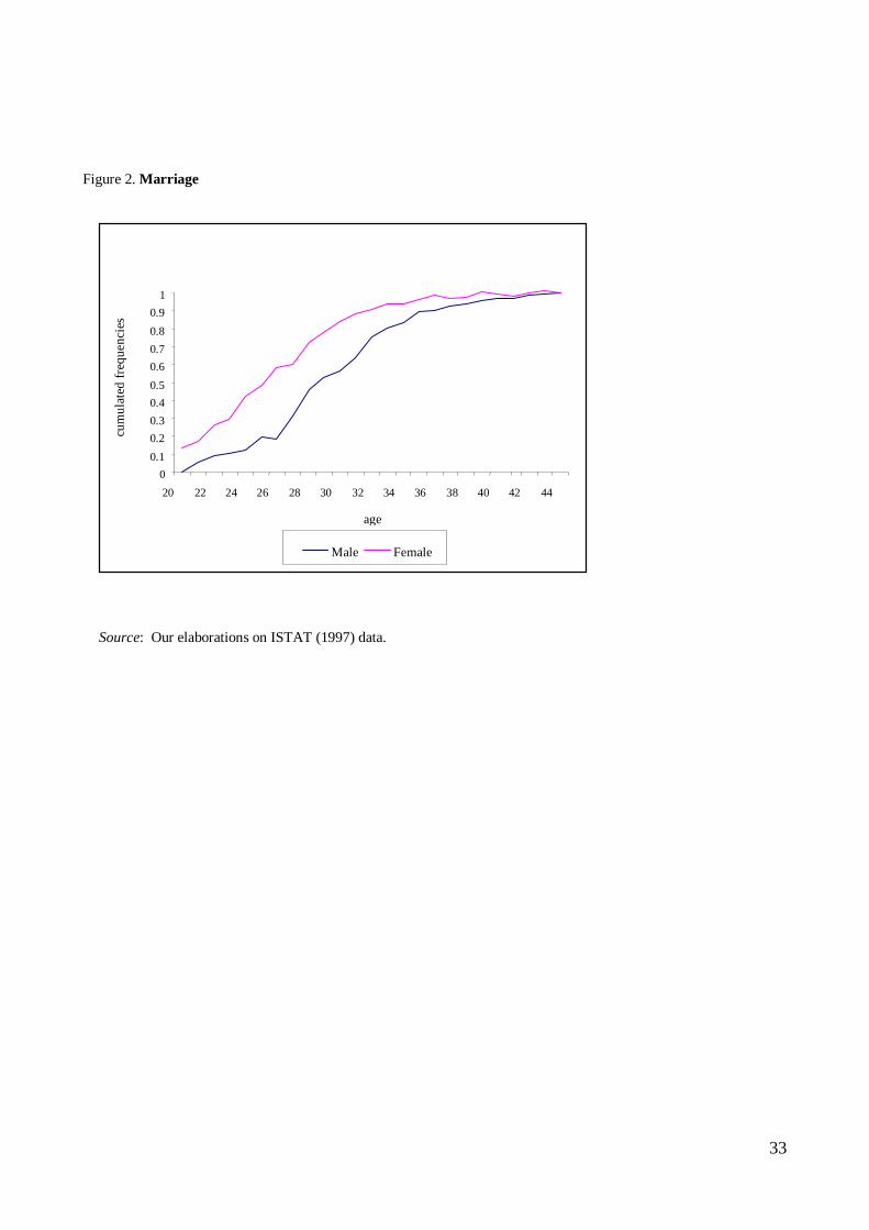
33
Figure 2. Marriage
Source: Our elaborations on ISTAT (1997) data.
0 0.1 0.2 0.3 0.4 0.5 0.6 0.7 0.8 0.9
1
20 22 24 26 28 30 32 34 36 38 40 42 44 age
cum
ulat
ed fr
eque
ncie
s
Male Female
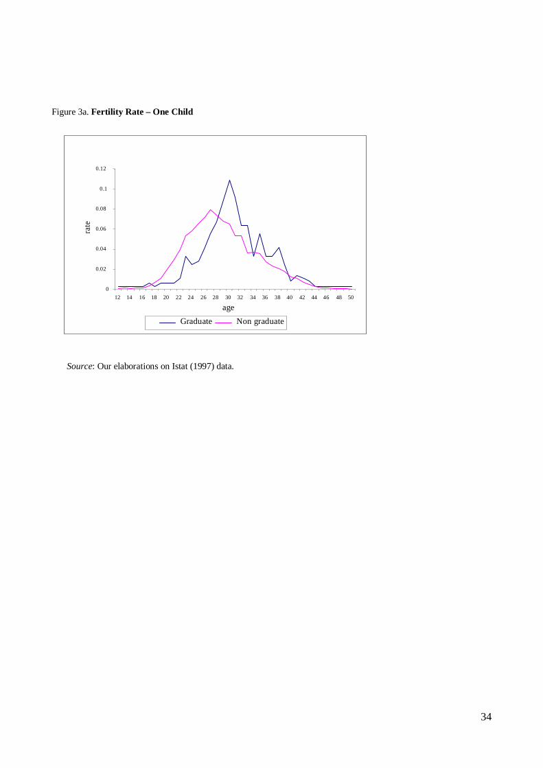
34
Figure 3a. Fertility Rate – One Child
Source: Our elaborations on Istat (1997) data.
0
0.02
0.04
0.06
0.08
0.1
0.12
12 14 16 18 20 22 24 26 28 30 32 34 36 38 40 42 44 46 48 50
age
rate
Graduate Non graduate

35
Figure 3b. Fertility Rate – Two Children (first child)
Source: Our elaborations on Istat (1997) data.
0
0 .02
0 .04
0 .06
0 .08
0.1
0 .12
0 .14
12 14 16 1 8 20 2 2 24 26 28 3 0 32 3 4 36 38 40 4 2 4 4 4 6 48 50
age
rate
G radua te N o n g radu ate

36
Figure 3c. Fertility Rate – Two Children (second child)
Source: Our elaborations on Istat (1997) data.
0
0 .02
0 .04
0 .06
0 .08
0 .1
0 .12
0 .14
12 14 1 6 1 8 20 22 2 4 26 28 3 0 32 34 3 6 38 40 42 44 46 48 50
a ge
rate
G ra d u ate N o n g ra d u a te
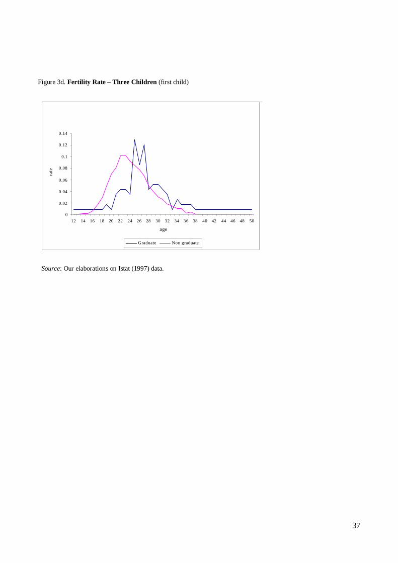
37
Figure 3d. Fertility Rate – Three Children (first child)
Source: Our elaborations on Istat (1997) data.
0
0.02
0.04
0.06
0.08
0.1
0.12
0.14
12 14 16 18 20 22 24 26 28 30 32 34 36 38 40 42 44 46 48 50
age
rate
Graduate Non graduate

38
Figure 3e. Fertility Rate – Three Children (second child)
Source: Our elaborations on Istat (1997) data.
0
0.01
0.02
0.03
0.04
0.05
0.06
0.07
0.08
0.09
0.1
12 14 16 18 20 22 24 26 28 30 32 34 36 38 40 42 44 46 48 50
age
rate
Graduate Non graduate

39
Figure 3f. Fertility Rate – Three Children (third child)
Source: Our elaborations on Istat (1997) data.
0
0.01
0.02
0.03
0.04
0.05
0.06
0.07
0.08
0.09
0.1
12 14 16 18 20 22 24 26 28 30 32 34 36 38 40 42 44 46 48 50
age
rate
Graduate Non graduate

40
Figure 4. Marginal Net Subsidy
45000
55000
65000
First Child Second Child Third Child
euro
s
Two Graduate Employees Single "Modal" "Average"
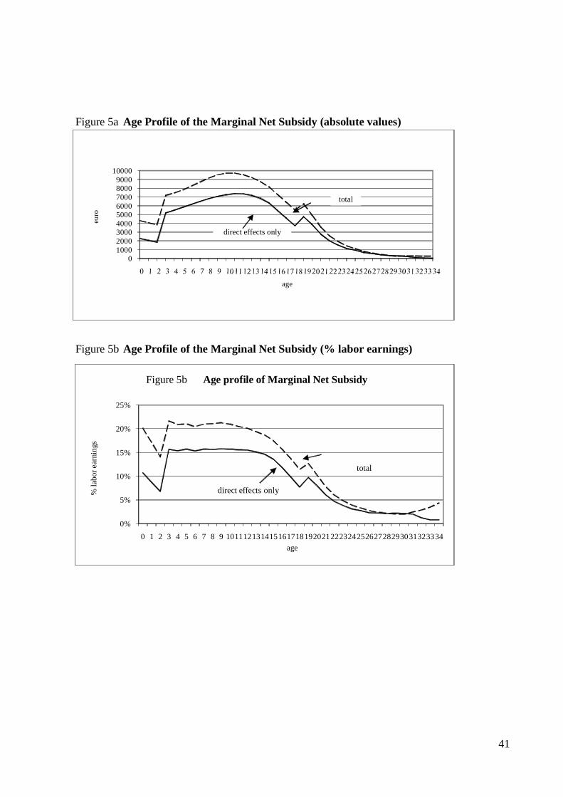
41
Figure 5a Age Profile of the Marginal Net Subsidy (absolute values)
Figure 5b Age Profile of the Marginal Net Subsidy (% labor earnings)
0100020003000400050006000700080009000
10000
euro
age
total
direct effects only
0%
5%
10%
15%
20%
25%
0 1 2 3 4 5 6 7 8 9 10111213141516171819202122232425262728293031323334
% la
bor e
arni
ngs
age
Figure 5b Age profile of Marginal Net Subsidy
total
direct effects only