Embed Size (px)
Citation preview
FAMILY ALGEBRAS AND THE ISOTYPIC COMPONENTS OF g⊗g
Matthew Tai
A DISSERTATION
in
Mathematics
Presented to the Faculties of the University of Pennsylvaniain
Partial Fulfillment of the Requirements for theDegree of Doctor of Philosophy
2014
Supervisor of Dissertation
Alexandre KirillovProfessor of Mathematics
Graduate Group Chairperson
David HarbaterProfessor of Mathematics
Dissertation Committee:Alexandre Kirillov, ProfessorTony Pantev, ProfessorWolfgang Ziller, Professor
All rights reserved
INFORMATION TO ALL USERSThe quality of this reproduction is dependent upon the quality of the copy submitted.
In the unlikely event that the author did not send a complete manuscriptand there are missing pages, these will be noted. Also, if material had to be removed,
a note will indicate the deletion.
Microform Edition © ProQuest LLC.All rights reserved. This work is protected against
unauthorized copying under Title 17, United States Code
ProQuest LLC.789 East Eisenhower Parkway
P.O. Box 1346Ann Arbor, MI 48106 - 1346
UMI 3623975Published by ProQuest LLC (2014). Copyright in the Dissertation held by the Author.
UMI Number: 3623975
Acknowledgments
I would like to thank Professor Alexandre Kirillov, my advisor, for both suggesting the
problem to me and for providing supervision and insight.
I would also like to thank Professors Wolfgang Ziller, Tony Pantev, Siddhartha Sahi, Jim
Lepowsky, Yi-Zhi Huang, Roe Goodman, Dana Ernst, Christian Stump and Richard
Green for advice, encouragement and inspiration.
Special thanks to Dmytro Yeroshkin for tremendous help, mathematically and compu-
tationally, and for listening to me complain about notation. I would also like to thank
his father Oleg Eroshkin for additional suggestions to ease computing.
Thanks as well to my friends and colleagues here at the UPenn math department, for
companionship and commiseration.
ii
ABSTRACT
FAMILY ALGEBRAS AND THE ISOTYPIC COMPONENTS OF g⊗g
Matthew Tai
Alexandre Kirillov
Given a complex simple Lie algebra g with adjoint group G , the space S(g) of poly-
nomials on g is isomorphic as a graded g-module to (I (g)⊗H(g) where I (g) = (S(g))G
is the space of G-invariant polynomials and H(g) is the space of G-harmonic poly-
nomials. For a representation V of g, the generalized exponents of V are given by∑k≥0
di m(Homg(V , Hk (g))qk . We define an algebra CV (g) = Homg(End(V ),S(g)) and
for the case of V = g we determine the structure of g using a combination of diagram-
matic methods and information about representations of the Weyl-group of g. We
find an almost uniform description of Cg(g) as an I (g)-algebra and as an I (g)-module
and from there determine the generalized exponents of the irreducible components
of End(g). The results support conjectures about (T (g))G , the G-invariant part of the
tensor algebra, and about a relation between generalized exponents and Lusztig’s fake
degrees.
iii
Contents
1 Introduction 1
1.1 Simple Lie Algebras and Exponents . . . . . . . . . . . . . . . . . . . . . . 1
1.2 Casimir Invariants . . . . . . . . . . . . . . . . . . . . . . . . . . . . . . . . 3
1.3 Generalized Exponents . . . . . . . . . . . . . . . . . . . . . . . . . . . . . . 5
2 Introduction to Family Algebras 7
2.1 Definition of Family Algebras . . . . . . . . . . . . . . . . . . . . . . . . . . 7
2.2 Relation to the Generalized Exponents . . . . . . . . . . . . . . . . . . . . 9
2.3 Restriction to the Cartan subalgebra . . . . . . . . . . . . . . . . . . . . . . 10
3 Results for V = g 12
3.1 Algebraic Structure . . . . . . . . . . . . . . . . . . . . . . . . . . . . . . . . 12
3.2 Fake Degrees . . . . . . . . . . . . . . . . . . . . . . . . . . . . . . . . . . . . 14
4 Diagrams 15
4.1 Casimir Operators and Structure Constants . . . . . . . . . . . . . . . . . 17
4.2 Projections . . . . . . . . . . . . . . . . . . . . . . . . . . . . . . . . . . . . . 19
iv
4.3 Symmetrization . . . . . . . . . . . . . . . . . . . . . . . . . . . . . . . . . . 19
5 Invariant Tensors 21
5.1 General Statement for most Classical Lie Algebras . . . . . . . . . . . . . . 21
5.2 Ar . . . . . . . . . . . . . . . . . . . . . . . . . . . . . . . . . . . . . . . . . . 22
5.3 Br . . . . . . . . . . . . . . . . . . . . . . . . . . . . . . . . . . . . . . . . . . 23
5.4 Cr . . . . . . . . . . . . . . . . . . . . . . . . . . . . . . . . . . . . . . . . . . 25
5.5 Other simple Lie algebras . . . . . . . . . . . . . . . . . . . . . . . . . . . . 26
6 The Ar case 28
6.1 Diagrams for Ar . . . . . . . . . . . . . . . . . . . . . . . . . . . . . . . . . . 28
6.2 Structure of the Family Algebra . . . . . . . . . . . . . . . . . . . . . . . . . 29
6.3 Sufficiency of the Generators . . . . . . . . . . . . . . . . . . . . . . . . . . 31
6.4 Proof of the Relations . . . . . . . . . . . . . . . . . . . . . . . . . . . . . . . 33
6.5 The Sufficiency of the Relations . . . . . . . . . . . . . . . . . . . . . . . . . 37
6.6 Generalized Exponents . . . . . . . . . . . . . . . . . . . . . . . . . . . . . . 40
7 The Br , Cr case 44
7.1 Diagrams . . . . . . . . . . . . . . . . . . . . . . . . . . . . . . . . . . . . . . 44
7.2 Generators . . . . . . . . . . . . . . . . . . . . . . . . . . . . . . . . . . . . . 46
7.3 Relations . . . . . . . . . . . . . . . . . . . . . . . . . . . . . . . . . . . . . . 48
7.4 Br . . . . . . . . . . . . . . . . . . . . . . . . . . . . . . . . . . . . . . . . . . 51
7.5 Generalized Exponents . . . . . . . . . . . . . . . . . . . . . . . . . . . . . . 53
v
8 The Dr case 56
8.1 Diagrams . . . . . . . . . . . . . . . . . . . . . . . . . . . . . . . . . . . . . . 56
8.2 Generators . . . . . . . . . . . . . . . . . . . . . . . . . . . . . . . . . . . . . 57
8.3 Sufficiency of the Generators . . . . . . . . . . . . . . . . . . . . . . . . . . 58
8.4 Relations . . . . . . . . . . . . . . . . . . . . . . . . . . . . . . . . . . . . . . 60
8.5 Generalized Exponents . . . . . . . . . . . . . . . . . . . . . . . . . . . . . . 63
9 Restrictions to Subalgebras 67
9.1 The Weyl Group Action . . . . . . . . . . . . . . . . . . . . . . . . . . . . . . 67
9.2 Restriction to Maximal Subalgebras . . . . . . . . . . . . . . . . . . . . . . 71
10 The Exceptional Lie algebras 75
10.1 Invariants . . . . . . . . . . . . . . . . . . . . . . . . . . . . . . . . . . . . . 75
10.2 The Decomposition of g⊗g . . . . . . . . . . . . . . . . . . . . . . . . . . . 76
10.3 General Structure . . . . . . . . . . . . . . . . . . . . . . . . . . . . . . . . . 77
10.4 Larger exceptional Lie algebras . . . . . . . . . . . . . . . . . . . . . . . . . 79
11 G2 82
12 F4 86
13 E6 94
14 E7 99
15 E8 104
vi
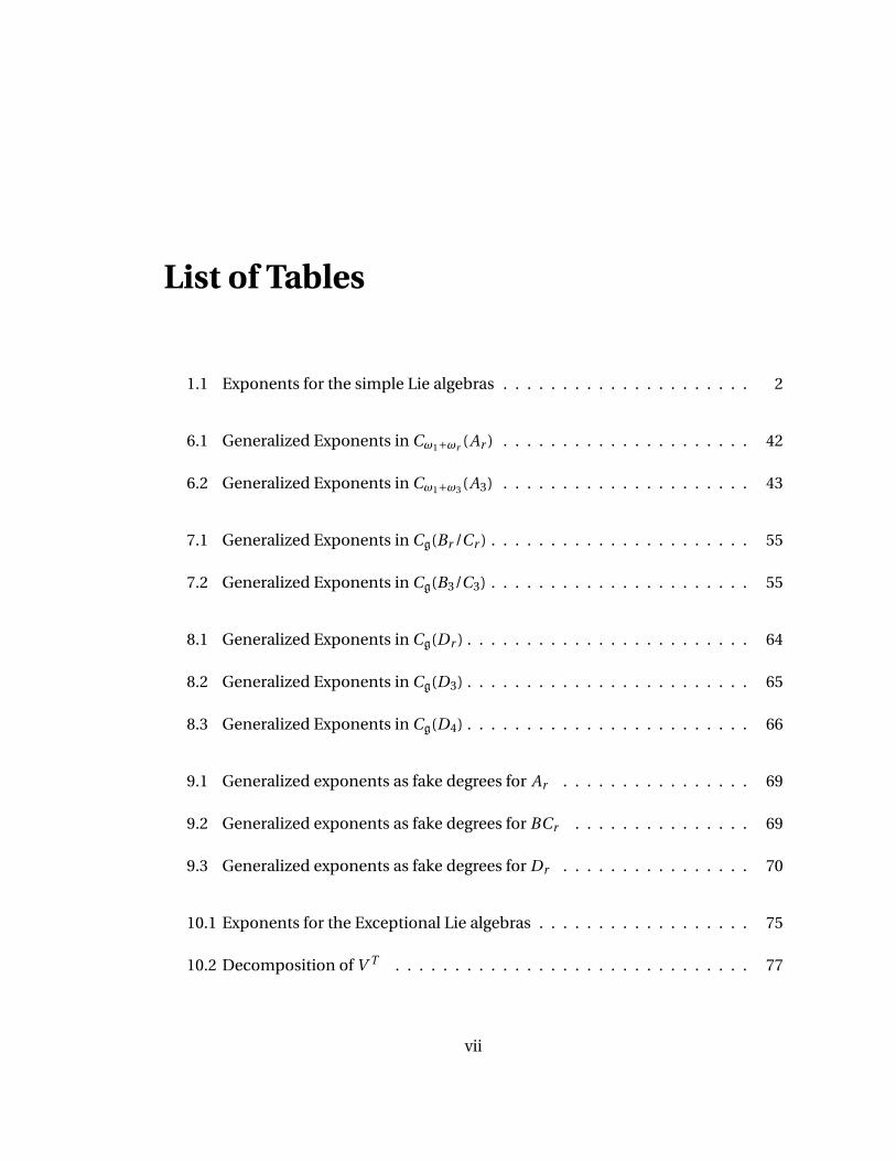
List of Tables
1.1 Exponents for the simple Lie algebras . . . . . . . . . . . . . . . . . . . . . 2
6.1 Generalized Exponents in Cω1+ωr (Ar ) . . . . . . . . . . . . . . . . . . . . . 42
6.2 Generalized Exponents in Cω1+ω3 (A3) . . . . . . . . . . . . . . . . . . . . . 43
7.1 Generalized Exponents in Cg(Br /Cr ) . . . . . . . . . . . . . . . . . . . . . . 55
7.2 Generalized Exponents in Cg(B3/C3) . . . . . . . . . . . . . . . . . . . . . . 55
8.1 Generalized Exponents in Cg(Dr ) . . . . . . . . . . . . . . . . . . . . . . . . 64
8.2 Generalized Exponents in Cg(D3) . . . . . . . . . . . . . . . . . . . . . . . . 65
8.3 Generalized Exponents in Cg(D4) . . . . . . . . . . . . . . . . . . . . . . . . 66
9.1 Generalized exponents as fake degrees for Ar . . . . . . . . . . . . . . . . 69
9.2 Generalized exponents as fake degrees for BCr . . . . . . . . . . . . . . . 69
9.3 Generalized exponents as fake degrees for Dr . . . . . . . . . . . . . . . . 70
10.1 Exponents for the Exceptional Lie algebras . . . . . . . . . . . . . . . . . . 75
10.2 Decomposition of V T . . . . . . . . . . . . . . . . . . . . . . . . . . . . . . 77
vii
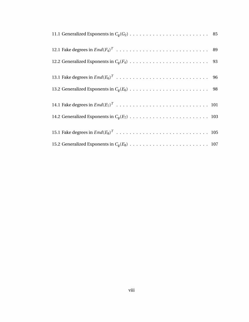
11.1 Generalized Exponents in Cg(G2) . . . . . . . . . . . . . . . . . . . . . . . . 85
12.1 Fake degrees in End(F4)T . . . . . . . . . . . . . . . . . . . . . . . . . . . . 89
12.2 Generalized Exponents in Cg(F4) . . . . . . . . . . . . . . . . . . . . . . . . 93
13.1 Fake degrees in End(E6)T . . . . . . . . . . . . . . . . . . . . . . . . . . . . 96
13.2 Generalized Exponents in Cg(E6) . . . . . . . . . . . . . . . . . . . . . . . . 98
14.1 Fake degrees in End(E7)T . . . . . . . . . . . . . . . . . . . . . . . . . . . . 101
14.2 Generalized Exponents in Cg(E7) . . . . . . . . . . . . . . . . . . . . . . . . 103
15.1 Fake degrees in End(E8)T . . . . . . . . . . . . . . . . . . . . . . . . . . . . 105
15.2 Generalized Exponents in Cg(E8) . . . . . . . . . . . . . . . . . . . . . . . . 107
viii
Chapter 1
Introduction
1.1 Simple Lie Algebras and Exponents
We consider the simple Lie algebras, these being the four classical series Ar ,Br ,Cr ,Dr
and the five exceptional algebras G2,F4,E6,E7,E8. Associated to each of these algebras
is a list of numbers called their exponents, which appear in a number of ways. The
name comes from the exponents of the hyperplane arrangement corresponding to the
simple reflection planes of the Weyl Group of the Lie algebra. The exponents can also
be considered topologically: for the compact group G associated to g, the Poincare
polynomial of G is
PG (q) = ∑k=0
r k(H k (G ,Z))qk =r∏
k=1(1+q2ek+1)
The simple Lie algebras are summarized in the following table, where the descriptions
of the exceptional Lie groups are based on the Rosenfeld projective planes [Ro97].
1
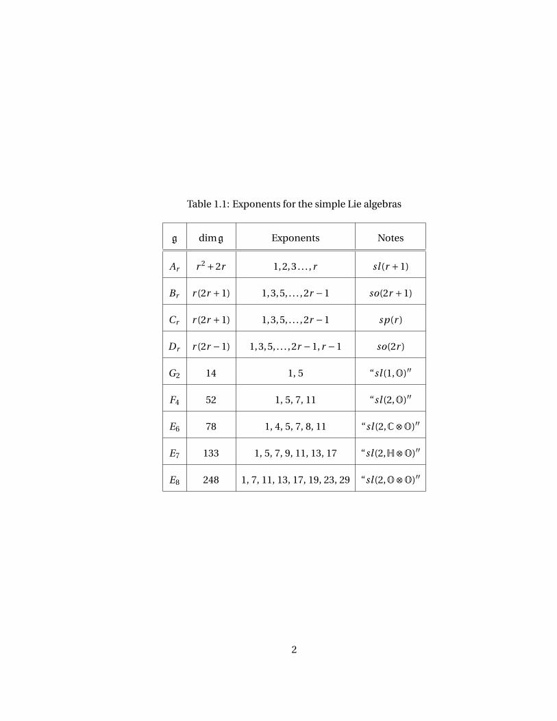
Table 1.1: Exponents for the simple Lie algebras
g dimg Exponents Notes
Ar r 2 +2r 1,2,3 . . . ,r sl (r +1)
Br r (2r +1) 1,3,5, . . . ,2r −1 so(2r +1)
Cr r (2r +1) 1,3,5, . . . ,2r −1 sp(r )
Dr r (2r −1) 1,3,5, . . . ,2r −1,r −1 so(2r )
G2 14 1, 5 “sl (1,O)′′
F4 52 1, 5, 7, 11 “sl (2,O)′′
E6 78 1, 4, 5, 7, 8, 11 “sl (2,C⊗O)′′
E7 133 1, 5, 7, 9, 11, 13, 17 “sl (2,H⊗O)′′
E8 248 1, 7, 11, 13, 17, 19, 23, 29 “sl (2,O⊗O)′′
2
1.2 Casimir Invariants
The exponents of g also have representation-theoretic interpretations. G acts on g via
the conjugation action, and hence on S(g), the symmetric algebra on g considered as
a vector space. We denote by I (g) the G-invariant subspace (S(g))G . In 1963, Kostant
showed that I (g) for simple g is a polynomial algebra where the number of generators
is equal to the rank of g, and that furthermore the degrees of these generators are each
one more than an exponent of g. For later use we establish a particular choice of gen-
erators of I (g), which we will call primitive Casimir operators.
For each Lie algebra, we pick a representation (V ,π) with which to define the primitive
Casimir operators. For sl (r +1) we pick one of the two r +1-dimensional representa-
tions. For so(n) we pick the n-dimensional representation, and for sp(r ) we pick the
2r -dimensional representation. For G2,F4,E6,E7, and E8 we pick the 7−,26−,27−,56−,
and 248−dimensional representations respectively. These are often also called the
“standard” representations, and with a few exceptions are the nontrivial representa-
tions of minimal dimension. From here on out, unless otherwise specified, V and π
refer to this defining representation.
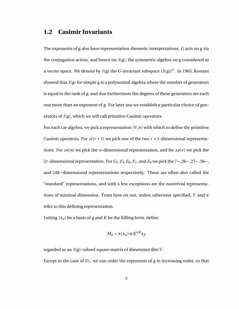
Letting {xα} be a basis of g and K be the Killing form, define
Md =π(xα)⊗K αβxβ
regarded as an S(g)-valued square matrix of dimension dimV .
Except in the case of Dr , we can order the exponents of g in increasing order, so that
3
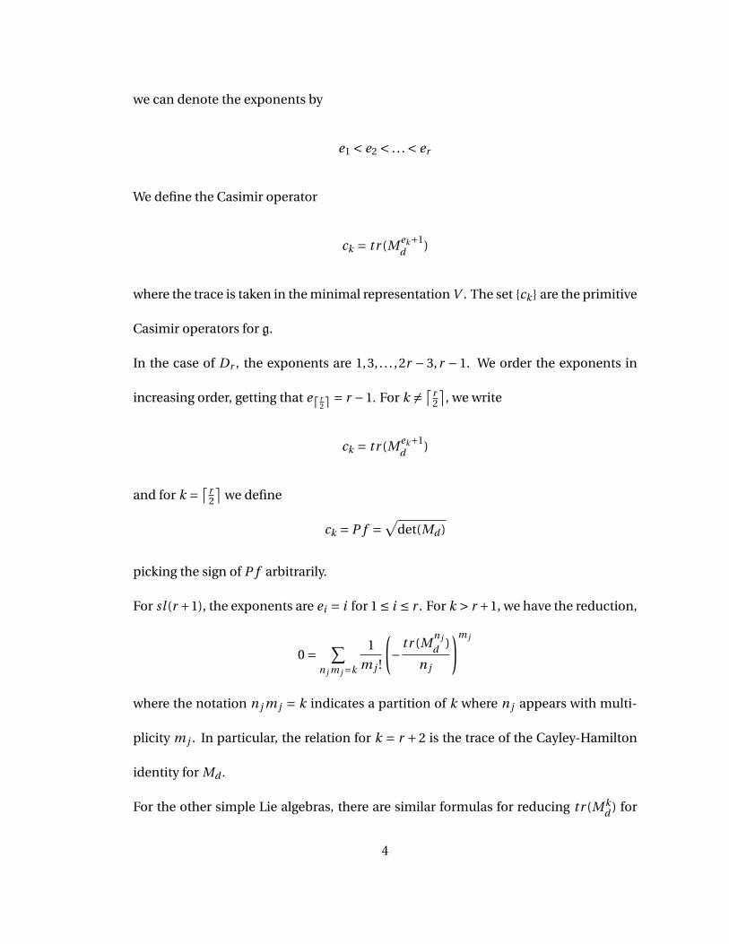
we can denote the exponents by
e1 < e2 < . . . < er
We define the Casimir operator
ck = tr (M ek+1d )
where the trace is taken in the minimal representation V . The set {ck } are the primitive
Casimir operators for g.
In the case of Dr , the exponents are 1,3, . . . ,2r − 3,r − 1. We order the exponents in
increasing order, getting that ed r2e = r −1. For k 6= ⌈ r
2
⌉, we write
ck = tr (M ek+1d )
and for k = ⌈ r2
⌉we define
ck = P f =√
det(Md )
picking the sign of P f arbitrarily.
For sl (r +1), the exponents are ei = i for 1 ≤ i ≤ r . For k > r +1, we have the reduction,
0 = ∑n j m j=k
1
m j !
(− tr (M
n j
d )
n j
)m j
where the notation n j m j = k indicates a partition of k where n j appears with multi-
plicity m j . In particular, the relation for k = r +2 is the trace of the Cayley-Hamilton
identity for Md .
For the other simple Lie algebras, there are similar formulas for reducing tr (M kd ) for
4
k not an exponent plus 1, with varying complexity. For the exceptional Lie algebras,
dim(V ) is much larger than er +1, so the Cayley-Hamilton identity doesn’t yield much
information about the how traces of low powers of Md reduce. See [RSV99] for details.
1.3 Generalized Exponents
In 1963, Kostant [Ko63] proved that for a representation V of g and hence of G , (V ⊗
S(g))G = HomG (V ∨,S(g)) is a free I (g) module. Thus we can find a basis for (V ⊗S(g))G
over I (g); Kostant calls the degrees of the polynomial components of this basis the gen-
eralized exponents of V (with multiplicity), usually expressed as a polynomial PV (q)
for a variable q . Note that for V = g, the generalized exponents for g match the classi-
cal notion of the exponents of g.
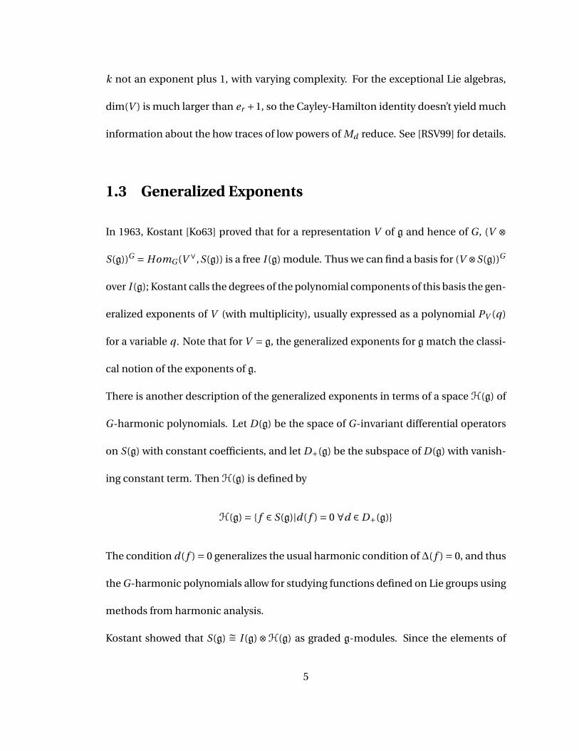
There is another description of the generalized exponents in terms of a space H(g) of
G-harmonic polynomials. Let D(g) be the space of G-invariant differential operators
on S(g) with constant coefficients, and let D+(g) be the subspace of D(g) with vanish-
ing constant term. Then H(g) is defined by
H(g) = { f ∈ S(g)|d( f ) = 0 ∀d ∈ D+(g)}
The condition d( f ) = 0 generalizes the usual harmonic condition of∆( f ) = 0, and thus
the G-harmonic polynomials allow for studying functions defined on Lie groups using
methods from harmonic analysis.
Kostant showed that S(g) ∼= I (g)⊗H(g) as graded g-modules. Since the elements of
5
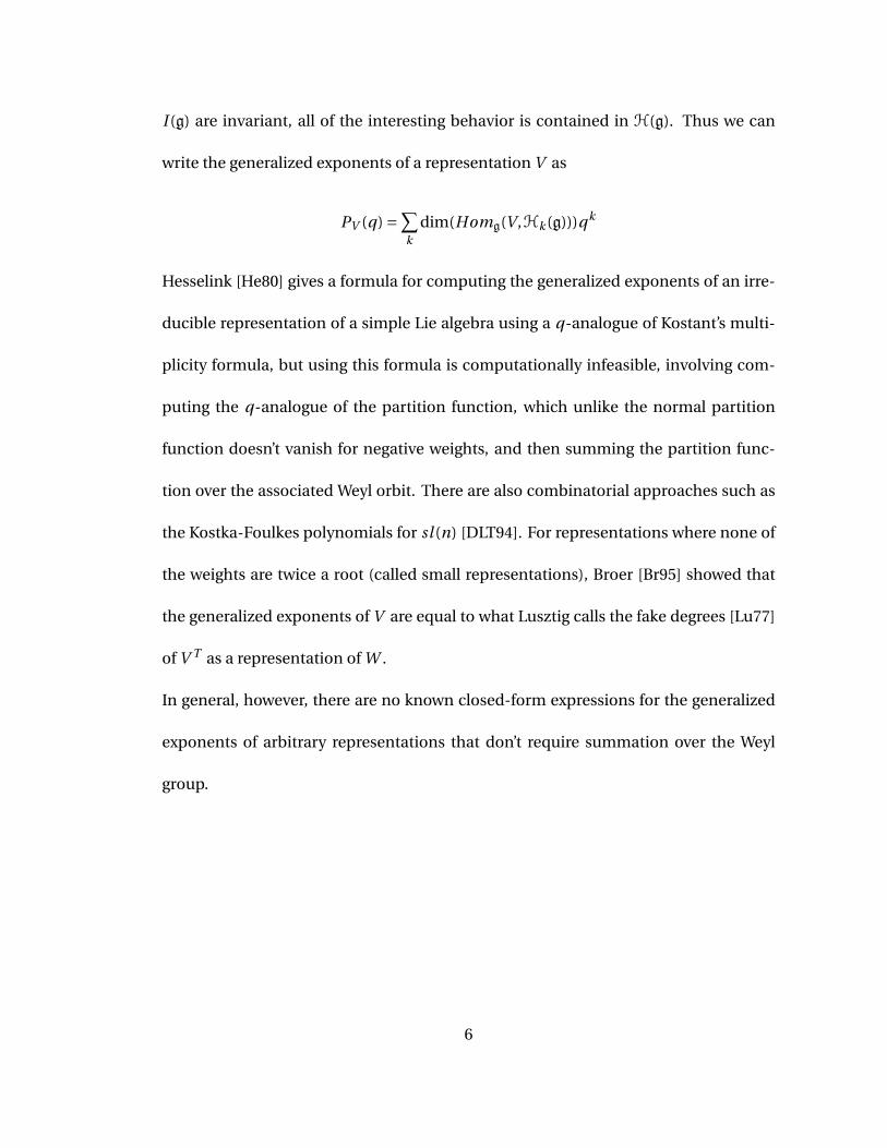
I (g) are invariant, all of the interesting behavior is contained in H(g). Thus we can
write the generalized exponents of a representation V as
PV (q) =∑k
dim(Homg(V ,Hk (g)))qk
Hesselink [He80] gives a formula for computing the generalized exponents of an irre-
ducible representation of a simple Lie algebra using a q-analogue of Kostant’s multi-
plicity formula, but using this formula is computationally infeasible, involving com-
puting the q-analogue of the partition function, which unlike the normal partition
function doesn’t vanish for negative weights, and then summing the partition func-
tion over the associated Weyl orbit. There are also combinatorial approaches such as
the Kostka-Foulkes polynomials for sl (n) [DLT94]. For representations where none of
the weights are twice a root (called small representations), Broer [Br95] showed that
the generalized exponents of V are equal to what Lusztig calls the fake degrees [Lu77]
of V T as a representation of W .
In general, however, there are no known closed-form expressions for the generalized
exponents of arbitrary representations that don’t require summation over the Weyl
group.
6
Chapter 2
Introduction to Family Algebras
2.1 Definition of Family Algebras
In [Ki00], Kirillov introduced what he calls Family Algebras in the hopes of providing
a new method for determining generalized exponents that doesn’t involve summing
over the Weyl group.
We fix a representation V of g and consider End(V ), with the conjugation action on it
induced from the action on V . We define the classical family algebra
CV (g) = (End(V )⊗S(g))G
where G is the adjoint group of g and acts by the action induced from g. This is an
algebra with multiplication ◦⊗m inherited from
◦ : End(V )⊗End(V ) → End(V )
7
via composition and
m : S(g)⊗S(g) → S(g)
via polynomial multiplication.
If we pick a basis {va} for V and let E ba be defined by E b
a vb = va , then we can write an
element of the family algebra as
E ba ⊗P a
b
where P ab ∈ S(g). We call the set {P a
b } the polynomial component of E ba ⊗P a
b . Note that
for two elements E ba ⊗P a
b and E ba ⊗Qa
b , the multiplication looks like
(E ba ⊗P a
b )× (E ba ⊗Qa
b ) = E ba ⊗P a
c Qcb
So the multiplication respects the natural grading on the polynomial components, and
hence we say that an element E ba ⊗P a
b is homogeneous of degree k if all of the {P ab } are
homogeneous of degree k.
The phrase “family algebra” comes from the decomposition of
End(V ) =⊕i
Vi
for irreducible Vi , which Kirillov calls the children of V . The family algebra CV (g) de-
composes similarly into
CV (g) =⊕i
(Vi ⊗S(g))G
Thus a family algebra gives us an I (g) module that is closed under multiplication and
is built from a finite set of isotypic components. Note that if Vi is a component of
8
End(V ), then so is V ∨i ; hence
CV (g) =⊕i
(Vi ⊗S(g))G ∼=⊕
iHomg(Vi ,S(g))
There is a natural quantization to what Kirillov calls the quantum family algebra,
QV (g) = (End(V )⊗U (g))G
U (g) is isomorphic to S(g) as G-modules, so there is a map that sends QV (g) to CV (g),
but the classical and quantum family algebras for a given V differ in their multiplica-
tive structures. This dissertation will only consider classical family algebras.
2.2 Relation to the Generalized Exponents
For an irreducible representation Vi , there is an I (g)-linear basis of Homg(Vi ,S(g))
where there is a bijection between generalized exponents ei j (with multiplicity) and
basis elements Ai j such that
Ai j ∈ Homg(Vi ,Hei j (g))
Hence, using the decomposition of End(V ) into irreducible representations, there is
an I (g)-linear basis of CV (g) where each basis element is in Homg(Vi ,Hei j (g)) for some
Vi in the decomposition of End(V ) and some ei j a generalized exponent of Vi .
Thus the general strategy of family algebras is to determine the algebraic structure of
a given family algebra, use that to determine an I (g)-linear basis, turn that basis into a
harmonic basis and from there compute the generalized exponents.
9
2.3 Restriction to the Cartan subalgebra
Given a Cartan subalgebra h of g with corresponding torus T ⊂G , we can look at S(h),
and in particular the restriction r es : S(g) → S(h) given by viewing the two algebras as
Pol [g∨] and Pol [h∨] respectively, and sending an element f ∈ S(g) to f |h∨ . While this
map is generally not an injection, there are some useful aspects. Chevalley’s restriction
theorem [Br95] says that
r es|I (g) : I (g) → I (h) = S(h)W
is an isomorphism. We get a map
Res : (V ⊗S(g))G → (V T ⊗S(h))W
induced by restricting from V to V T and from S(g) to S(h), which Kostant shows is
an injection. The result by Broer mentioned in the first chapter is a necessary and
sufficient condition for Res to be an isomorphism.
Writing BV (h) for End(V )T ⊗S(h) we get that
Res : CV (g) → BV (h)W
is an injection. We can make Res into a surjection by localizing with respect to the
non-zero part of I (g). In particular, let K0 be the fraction field of I (g) ∼= S(h)W . Then by
[Ki01] we have that
CV (g)⊗I (g) K0∼= BV (h)W ⊗I (h) K0
10
This then tells us that the dimension of CV (g) over I (g) is equal to the dimension of
BV (h)W over I (h).
End(V )T = ⊕µ∈W t (V )
M atmV (µ)(C)
and so BV (h)W is the W -invariant subalgebra of the sum of matrix algebras
⊕µ∈W t (V )
M atmV (µ)(S(h))
Since the multiplicity over I (h) of a representation φ of W in S(h) is dim(φ), the di-
mension of BV (h)W over I (h), i.e. the dimension of CV (g), is given by the sum of the
dimensions of the matrix algebras:
∑µ∈W t (V )
mV (µ)2
Given a weight λ ∈ W t (V ), we can consider an element of BV (h)W that is the identity
on the matrix algebras corresponding to weights in W.λ and vanish elsewhere. Such
an element lifts to an element of CV (g) which, for some P ∈ I (h), restricts to P times the
identity on the matrix algebras corresponding to weights in W.λ and vanish elsewhere.
We can use these elements of CV (g) as analogues to projection operators.
11
Chapter 3
Results for V = g
This dissertation will focus on the particular case of the adjoint representation, i.e. set-
ting V = g. The weights in question are then the roots of g as well as 0 with multiplicity
r , where r is the rank of g. We denote the image of (End(g)T ⊗S(h))W in M atr (S(h)) by
the torus part of the algebra, and everything else by the vector part, as it is composed
of 1-dimensional and hence scalar algebras. Note that the vector part is commutative,
since S(h) is commutative, so any non-commutativity in the family algebra appears
only in the torus part.
3.1 Algebraic Structure
The decomposition of End(g) into irreducible components depends on g, but is uni-
form for all of the An , uniform for Bn ,Cn and Dn , and is uniform for the five excep-
tional Lie algebras [CV08]. The main result of this dissertation is that though the form
12
of Cg(g) as a g-module ends up quite different, the algebraic structures of Cg(g) are
very similar for all of the simple Lie algebras. There are two generators common to
all of family algebras in question, denoted M and S, and then a set of r other gener-
ators, labelled R1 through Rr , that depend on the structure of g. A set of I (g)-linearly
independent basis elements of Cg(g) is then
M mRk for 0 ≤ m ≤ er +1,1 ≤ k ≤ r
RmSRn +RnSRm for 1 ≤ m ≤ n ≤ r −1
RmSRn −RnSRm for 1 ≤ m < n ≤ r
Here R1 is a scalar, left in for uniformity of expression.
The Rk can themselves be generated by either M ,S and R2 in the cases of Ar ,Br ,Cr
and G2, by M ,S,R2 and Rr for Dr , or by M ,S,R2 and R3.in the cases of F4,E6,E7 and
E8.
There are several relations common to all of the cases. The terms M mRk for m ≥ 1
vanish on the torus part, and any term involving S vanishes on the vector part. Hence
M is central and MS = SM = 0. The Rk commute with each other and with M , but
not with S. SRk S = Pk S for some Pk ∈ I (g), although the form of Pk depends on g.
The relations describing the products of the Rk also depend on g, in particular the
existence or absence of primitive Casimir elements in particular degrees.
13
3.2 Fake Degrees
For the Weyl group W acting on the Cartan subalgebra h, there is a notion called “fake
degrees” analogous to that of the generalized exponents, in that there is a polyno-
mial PU (q) describing the maps from a W -representation U into a space M(h) of W -
harmonic polynomials. For the representations relevant to g⊗g, we have the following
statement: if V T =⊕iUi as W -modules, then
PV (q) =∑i
qki PUi (q)
for some set of exponents ki , although the ki are not uniquely determined.
For each classical families there are uniform expressions for the qi in terms of r , as
well as for the Er family.
14
Chapter 4
Diagrams
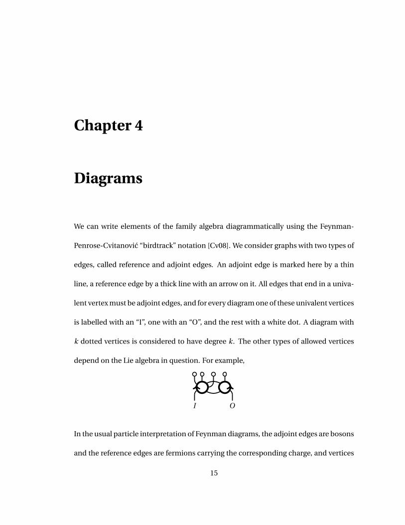
We can write elements of the family algebra diagrammatically using the Feynman-
Penrose-Cvitanovic “birdtrack” notation [Cv08]. We consider graphs with two types of
edges, called reference and adjoint edges. An adjoint edge is marked here by a thin
line, a reference edge by a thick line with an arrow on it. All edges that end in a univa-
lent vertex must be adjoint edges, and for every diagram one of these univalent vertices
is labelled with an “I”, one with an “O”, and the rest with a white dot. A diagram with
k dotted vertices is considered to have degree k. The other types of allowed vertices
depend on the Lie algebra in question. For example,
I O
In the usual particle interpretation of Feynman diagrams, the adjoint edges are bosons
and the reference edges are fermions carrying the corresponding charge, and vertices
15
of valence higher than 1 being interactions, with G being the gauge group of the inter-
actions. Momentum constraints are ignored here.
In the Lie algebra interpretation, the reference edges correspond to copies of the ref-
erence representation, the adjoint edges are copies of the adjoint representation, and
vertices of valence higher than 1 are invariants. In particular, the vertices with one
reference edge pointing in, one reference edge pointing out and one adjoint edge at-
tached are Clebsches for V ⊗V ∨ → Ad j . In the standard index notation for tensors,
each vertex is an invariant tensor with an upper reference index for each arrow going
in, a lower reference index for each arrow going out, and an adjoint index for each ad-
joint edge attached; two indices are contracted if they are connected by an edge. The
ability to turn upper adjoint indices into lower adjoint indices via the Killing form al-
lows us to not require arrows on the adjoint edges.
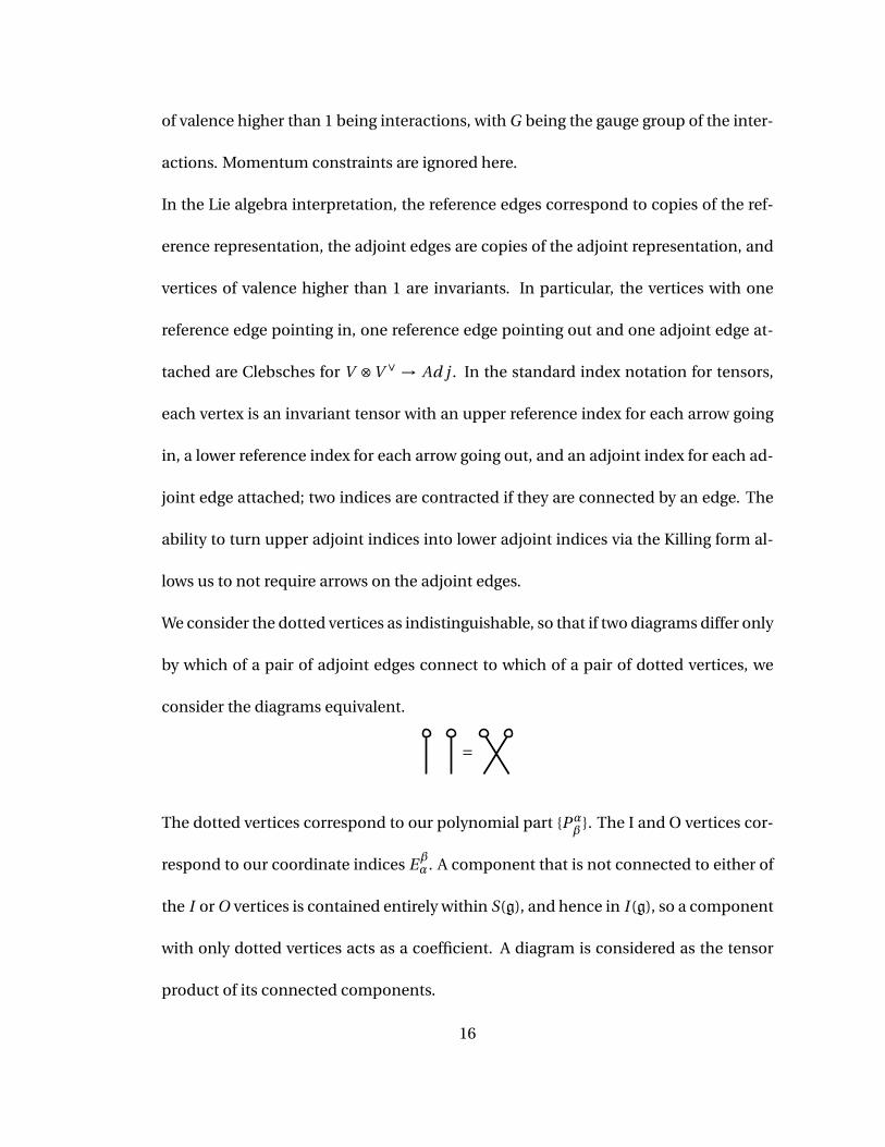
We consider the dotted vertices as indistinguishable, so that if two diagrams differ only
by which of a pair of adjoint edges connect to which of a pair of dotted vertices, we
consider the diagrams equivalent.
=
The dotted vertices correspond to our polynomial part {Pαβ
}. The I and O vertices cor-
respond to our coordinate indices Eβα. A component that is not connected to either of
the I or O vertices is contained entirely within S(g), and hence in I (g), so a component
with only dotted vertices acts as a coefficient. A diagram is considered as the tensor
product of its connected components.
16
These diagrams are all naturally G-invariant, being built out of G-invariant objects,
and hence all diagrams are naturally in (End(g)⊗S(g))G . Thus any diagram as defined
above automatically gives a family algebra element, as opposed to the initial setup of
defining End(g)⊗S(g) and then imposing g-invariance as an additional property. By
Cvitanovic, all elements of the family algebra are formalC-linear combinations of such
diagrams, so we can consider the algebra in terms of these diagrams.
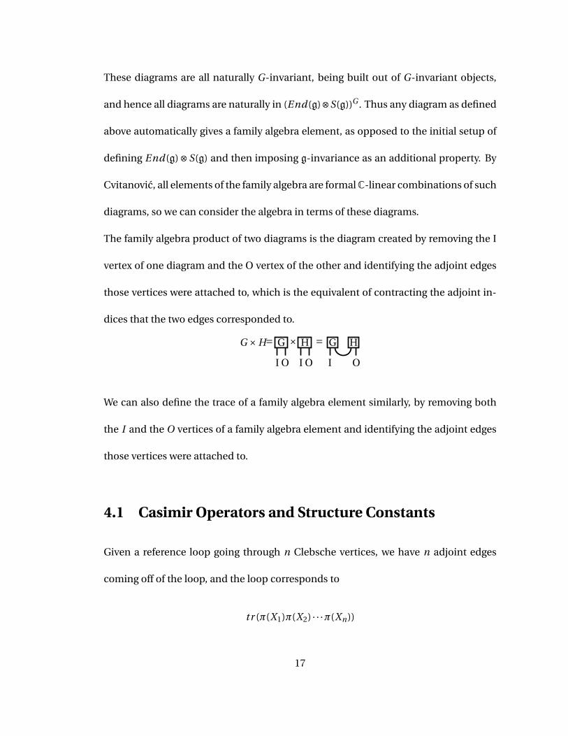
The family algebra product of two diagrams is the diagram created by removing the I
vertex of one diagram and the O vertex of the other and identifying the adjoint edges
those vertices were attached to, which is the equivalent of contracting the adjoint in-
dices that the two edges corresponded to.
G ×H= G
I O
× H
I O
= G
I
H
O
We can also define the trace of a family algebra element similarly, by removing both
the I and the O vertices of a family algebra element and identifying the adjoint edges
those vertices were attached to.
4.1 Casimir Operators and Structure Constants
Given a reference loop going through n Clebsche vertices, we have n adjoint edges
coming off of the loop, and the loop corresponds to
tr (π(X1)π(X2) · · ·π(Xn))
17
where the Xi are the adjoint edges, i.e. elements of g. As such, a loop of reference
edges going through k Clebsche vertices will be called a “trace” of order k from now
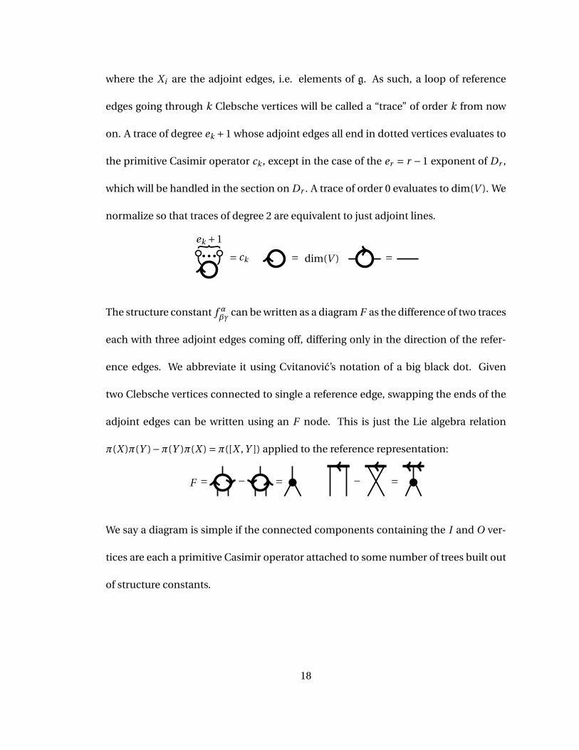
on. A trace of degree ek +1 whose adjoint edges all end in dotted vertices evaluates to
the primitive Casimir operator ck , except in the case of the er = r −1 exponent of Dr ,
which will be handled in the section on Dr . A trace of order 0 evaluates to dim(V ). We
normalize so that traces of degree 2 are equivalent to just adjoint lines.
ek +1
= ck = dim(V ) =
The structure constant f αβγ
can be written as a diagram F as the difference of two traces
each with three adjoint edges coming off, differing only in the direction of the refer-
ence edges. We abbreviate it using Cvitanovic’s notation of a big black dot. Given
two Clebsche vertices connected to single a reference edge, swapping the ends of the
adjoint edges can be written using an F node. This is just the Lie algebra relation
π(X )π(Y )−π(Y )π(X ) =π([X ,Y ]) applied to the reference representation:
F = − = − =
We say a diagram is simple if the connected components containing the I and O ver-
tices are each a primitive Casimir operator attached to some number of trees built out
of structure constants.
18
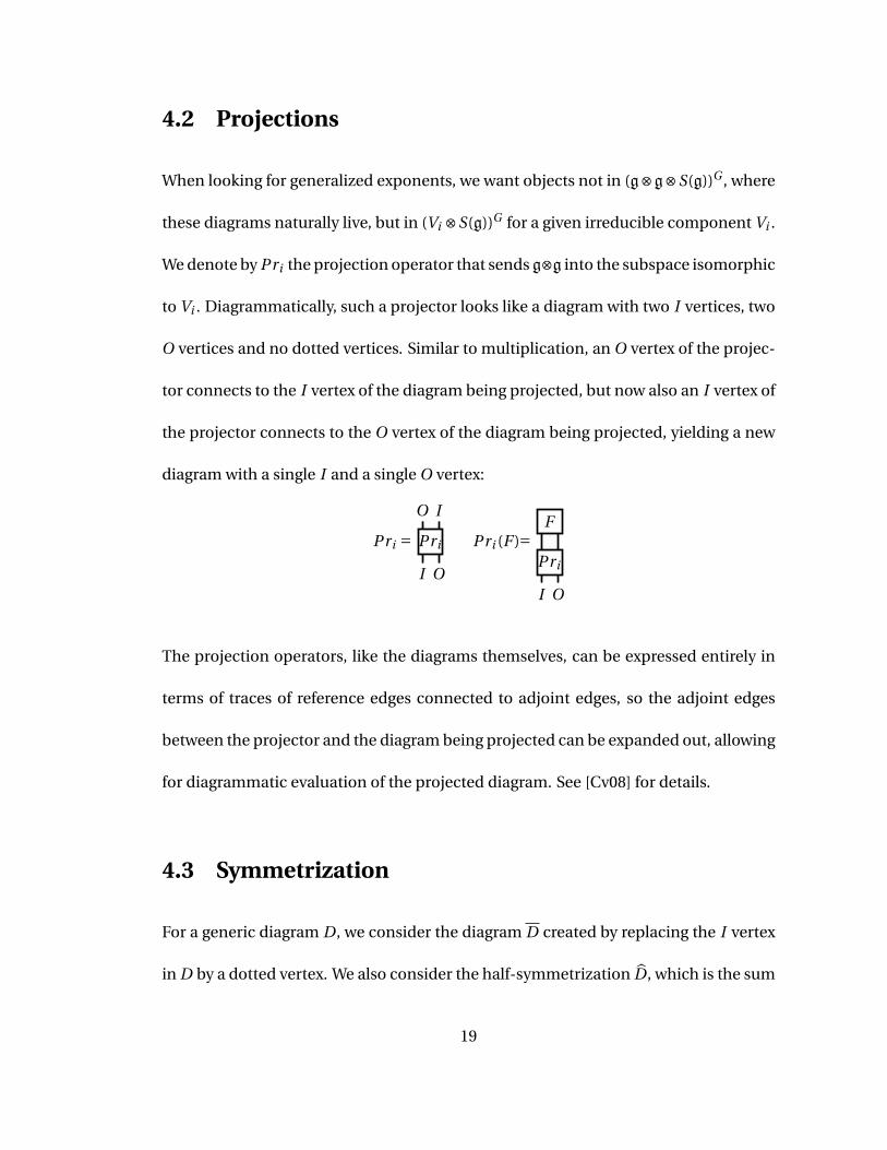
4.2 Projections
When looking for generalized exponents, we want objects not in (g⊗g⊗S(g))G , where
these diagrams naturally live, but in (Vi ⊗S(g))G for a given irreducible component Vi .
We denote by Pri the projection operator that sends g⊗g into the subspace isomorphic
to Vi . Diagrammatically, such a projector looks like a diagram with two I vertices, two
O vertices and no dotted vertices. Similar to multiplication, an O vertex of the projec-
tor connects to the I vertex of the diagram being projected, but now also an I vertex of
the projector connects to the O vertex of the diagram being projected, yielding a new
diagram with a single I and a single O vertex:
Pri = Pri
I O
O I
Pri (F )=Pri
F
I O
The projection operators, like the diagrams themselves, can be expressed entirely in
terms of traces of reference edges connected to adjoint edges, so the adjoint edges
between the projector and the diagram being projected can be expanded out, allowing
for diagrammatic evaluation of the projected diagram. See [Cv08] for details.
4.3 Symmetrization
For a generic diagram D , we consider the diagram D created by replacing the I vertex
in D by a dotted vertex. We also consider the half-symmetrization D , which is the sum
19
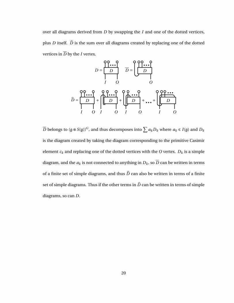
over all diagrams derived from D by swapping the I and one of the dotted vertices,
plus D itself. D is the sum over all diagrams created by replacing one of the dotted
vertices in D by the I vertex.
D = D
I O
D = D
O
D = D
I O
+ D
I O
+ D
I O
+ +
I
D
O
D belongs to (g⊗S(g))G , and thus decomposes into∑
ak Dk where ak ∈ I (g) and Dk
is the diagram created by taking the diagram corresponding to the primitive Casimir
element ck and replacing one of the dotted vertices with the O vertex. Dk is a simple
diagram, and the ak is not connected to anything in Dk , so D can be written in terms
of a finite set of simple diagrams, and thus D can also be written in terms of a finite
set of simple diagrams. Thus if the other terms in D can be written in terms of simple
diagrams, so can D .
20
Chapter 5
Invariant Tensors
5.1 General Statement for most Classical Lie Algebras
For Ar , Br and Cr there is a particularly elegant expression for all the elements of the
invariant tensors (T (g))G coming from the reference representations.
Theorem 5.1.1 (Invariant Tensors for Ar ,Br and Cr ). For g= Ar ,Br or Cr with the cor-
responding reference representation (V ,π), the elements of (T (g))G can be expressed as
tensor products of
trV (π(Xα1 )π(Xα2 ) · · ·π(Xαk ))Xα1 ⊗Xα2 ⊗·· ·⊗Xαk ∈ T (g)
along with permutations of the indices.
Diagrammatically, this corresponds to the statement that all diagrams with only
adjoint edges leaving the diagram are expressible as loops over the reference repre-
21
sentation with adjoint edges attached, where no two loops are connected by an adjoint
edge.
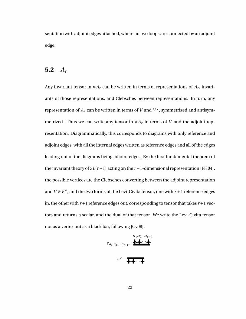
5.2 Ar
Any invariant tensor in ⊗Ar can be written in terms of representations of Ar , invari-
ants of those representations, and Clebsches between representations. In turn, any
representation of Ar can be written in terms of V and V ∨, symmetrized and antisym-
metrized. Thus we can write any tensor in ⊗Ar in terms of V and the adjoint rep-
resentation. Diagrammatically, this corresponds to diagrams with only reference and
adjoint edges, with all the internal edges written as reference edges and all of the edges
leading out of the diagrams being adjoint edges. By the first fundamental theorem of
the invariant theory of SL(r+1) acting on the r+1-dimensional representation [FH04],
the possible vertices are the Clebsches converting between the adjoint representation
and V ⊗V ∨, and the two forms of the Levi-Civita tensor, one with r +1 reference edges
in, the other with r+1 reference edges out, corresponding to tensor that takes r+1 vec-
tors and returns a scalar, and the dual of that tensor. We write the Levi-Civita tensor
not as a vertex but as a black bar, following [Cv08]:
εa1,a2,...,ar+1=a1a2
. . .ar+1
ε∨= . . .
22
Since the only edges that can lead out of the diagram have to be adjoint edges, corre-
sponding to the fact that all of our tensors are in T (Ar ), any instance of the Levi-Civita
tensor in the tensor must be matched by an instance of the dual of the Levi-Civita ten-
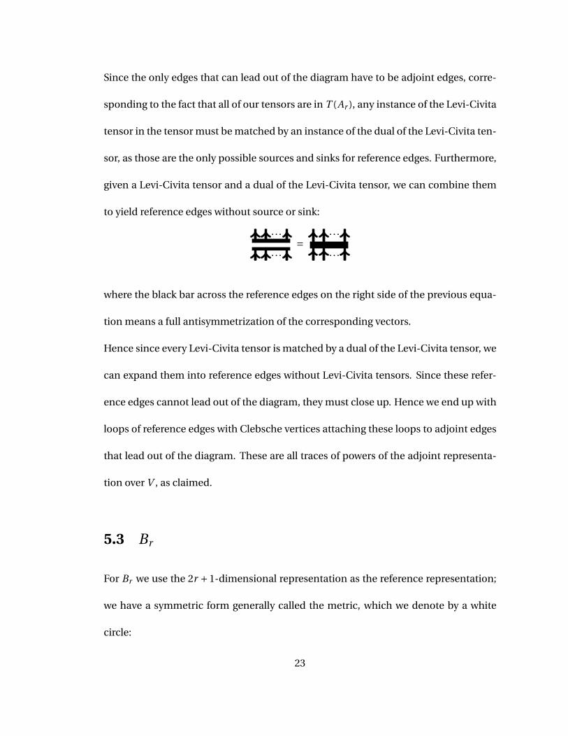
sor, as those are the only possible sources and sinks for reference edges. Furthermore,
given a Levi-Civita tensor and a dual of the Levi-Civita tensor, we can combine them
to yield reference edges without source or sink:
. . .
. . .=
. . .
. . .
where the black bar across the reference edges on the right side of the previous equa-
tion means a full antisymmetrization of the corresponding vectors.
Hence since every Levi-Civita tensor is matched by a dual of the Levi-Civita tensor, we
can expand them into reference edges without Levi-Civita tensors. Since these refer-
ence edges cannot lead out of the diagram, they must close up. Hence we end up with
loops of reference edges with Clebsche vertices attaching these loops to adjoint edges
that lead out of the diagram. These are all traces of powers of the adjoint representa-
tion over V , as claimed.
5.3 Br
For Br we use the 2r +1-dimensional representation as the reference representation;
we have a symmetric form generally called the metric, which we denote by a white
circle:
23
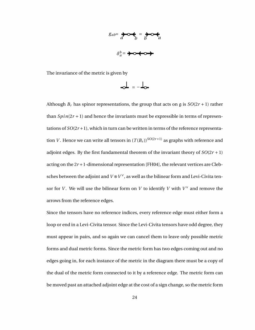
gab=a b
=b a
δba =
The invariance of the metric is given by
= −
Although Br has spinor representations, the group that acts on g is SO(2r +1) rather
than Spi n(2r +1) and hence the invariants must be expressible in terms of represen-
tations of SO(2r +1), which in turn can be written in terms of the reference representa-
tion V . Hence we can write all tensors in (T (Br ))SO(2r+1) as graphs with reference and
adjoint edges. By the first fundamental theorem of the invariant theory of SO(2r +1)
acting on the 2r +1-dimensional representation [FH04], the relevant vertices are Cleb-
sches between the adjoint and V ⊗V ∨, as well as the bilinear form and Levi-Civita ten-
sor for V . We will use the bilinear form on V to identify V with V ∨ and remove the
arrows from the reference edges.
Since the tensors have no reference indices, every reference edge must either form a
loop or end in a Levi-Civita tensor. Since the Levi-Civita tensors have odd degree, they
must appear in pairs, and so again we can cancel them to leave only possible metric
forms and dual metric forms. Since the metric form has two edges coming out and no
edges going in, for each instance of the metric in the diagram there must be a copy of
the dual of the metric form connected to it by a reference edge. The metric form can
be moved past an attached adjoint edge at the cost of a sign change, so the metric form
24
and its dual can be placed next to each other and thus cancelled. Hence all instances
of the metric forms and its dual can be removed from a diagram in (T (Br ))SO(2r+1),
leaving only loops in the reference representation attached to adjoint edges.
5.4 Cr
For Cr , all representations of Sp(r ) can be written in terms of the 2r -dimensional rep-
resentation. By the first fundamental theorem of the invariant theory of SO(2r +1) act-
ing on the 2r +1-dimensional representation [FH04], the relevant vertices for the 2r -
dimensional representation are the Clebsches and the symplectic form and its dual.
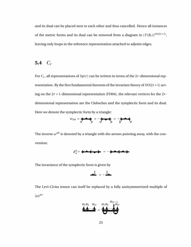
Here we denote the symplectic form by a triangle:
ωab =a b
= −a b
= −b a
The inverse ωab is denoted by a triangle with the arrows pointing away, with the con-
vention:
δba = = −
The invariance of the symplectic form is given by
= −
The Levi-Civita tensor can itself be replaced by a fully antisymmetrized multiple of
(ω)⊗r
a1a2. . .
a2r
=a1a2
. . .
. . .
a2r−1a2r
25
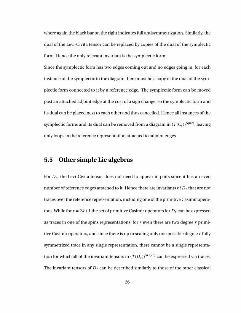
where again the black bar on the right indicates full antisymmetrization. Similarly, the
dual of the Levi-Civita tensor can be replaced by copies of the dual of the symplectic
form. Hence the only relevant invariant is the symplectic form.
Since the symplectic form has two edges coming out and no edges going in, for each
instance of the symplectic in the diagram there must be a copy of the dual of the sym-
plectic form connected to it by a reference edge. The symplectic form can be moved
past an attached adjoint edge at the cost of a sign change, so the symplectic form and
its dual can be placed next to each other and thus cancelled. Hence all instances of the
symplectic forms and its dual can be removed from a diagram in (T (Cr ))Sp(r ), leaving
only loops in the reference representation attached to adjoint edges.
5.5 Other simple Lie algebras
For Dr , the Levi-Civita tensor does not need to appear in pairs since it has an even
number of reference edges attached to it. Hence there are invariants of Dr that are not
traces over the reference representation, including one of the primitive Casimir opera-
tors. While for r = 2k+1 the set of primitive Casimir operators for Dr can be expressed
as traces in one of the spins representations, for r even there are two degree r primi-
tive Casimir operators, and since there is up to scaling only one possible degree r fully
symmetrized trace in any single representation, there cannot be a single representa-
tion for which all of the invariant tensors in (T (Dr ))SO(2r ) can be expressed via traces.
The invariant tensors of Dr can be described similarly to those of the other classical
26
Lie algebras, but due to these complications will be handled in the chapter on Dr .
For the exceptional Lie algebras, the author conjectures that the statement given above
does hold for them, but the above methods for showing such do not work due to the
existence of higher-order invariants in their reference representations that do not van-
ish as simply as the ones for Ar , Br and Cr .
27
Chapter 6
The Ar case
As an example, we will use the case of A3, as A1 and A2 have been fully worked out in
[Ro01].
6.1 Diagrams for Ar
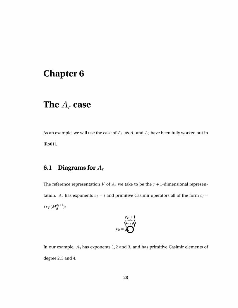
The reference representation V of Ar we take to be the r + 1-dimensional represen-
tation. Ar has exponents ei = i and primitive Casimir operators all of the form ci =
trV (M ei+1d ):
ck =
ek +1
In our example, A3 has exponents 1,2 and 3, and has primitive Casimir elements of
degree 2,3 and 4.
28
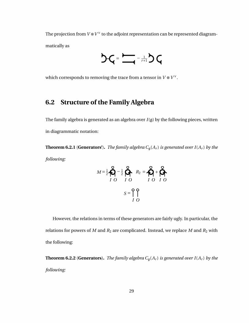
The projection from V ⊗V ∨ to the adjoint representation can be represented diagram-
matically as
= − 1r+1
which corresponds to removing the trace from a tensor in V ⊗V ∨.
6.2 Structure of the Family Algebra
The family algebra is generated as an algebra over I (g) by the following pieces, written
in diagrammatic notation:
Theorem 6.2.1 (Generators’). The family algebra Cg(Ar ) is generated over I (Ar ) by the
following:
M = 12
I O
− 12
I O
R2 =I O
+I O
S =I O
However, the relations in terms of these generators are fairly ugly. In particular, the
relations for powers of M and R2 are complicated. Instead, we replace M and R2 with
the following:
Theorem 6.2.2 (Generators). The family algebra Cg(Ar ) is generated over I (Ar ) by the
following:
29
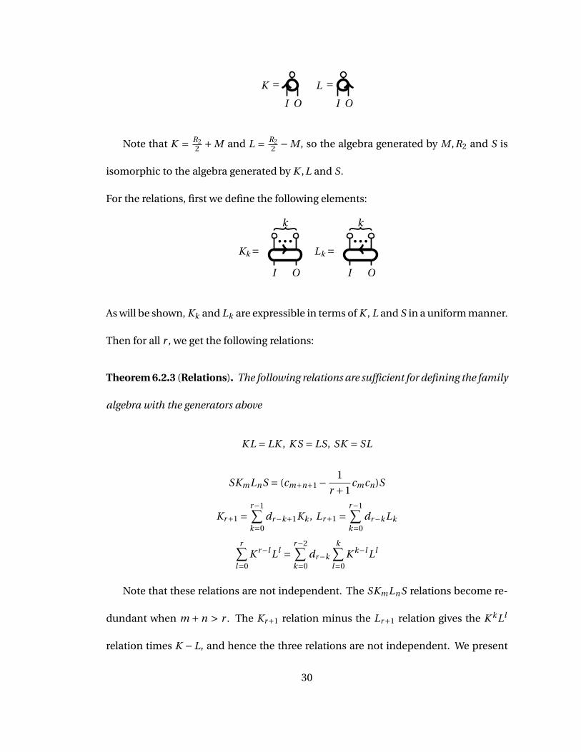
K =I O
L =I O
Note that K = R22 +M and L = R2
2 −M , so the algebra generated by M ,R2 and S is
isomorphic to the algebra generated by K ,L and S.
For the relations, first we define the following elements:
Kk=I O
k
Lk =I O
k
As will be shown, Kk and Lk are expressible in terms of K , L and S in a uniform manner.
Then for all r , we get the following relations:
Theorem 6.2.3 (Relations). The following relations are sufficient for defining the family
algebra with the generators above
K L = LK , K S = LS, SK = SL
SKmLnS = (cm+n+1 − 1
r +1cmcn)S
Kr+1 =r−1∑k=0
dr−k+1Kk , Lr+1 =r−1∑k=0
dr−k Lk
r∑l=0
K r−l Ll =r−2∑k=0
dr−k
k∑l=0
K k−l Ll
Note that these relations are not independent. The SKmLnS relations become re-
dundant when m +n > r . The Kr+1 relation minus the Lr+1 relation gives the K k Ll
relation times K −L, and hence the three relations are not independent. We present
30
both the Kr+1 and the Lr+1 relation because each of them is easier to prove individu-
ally than any linear combination of them that isn’t a multiple of the K k Ll relation.
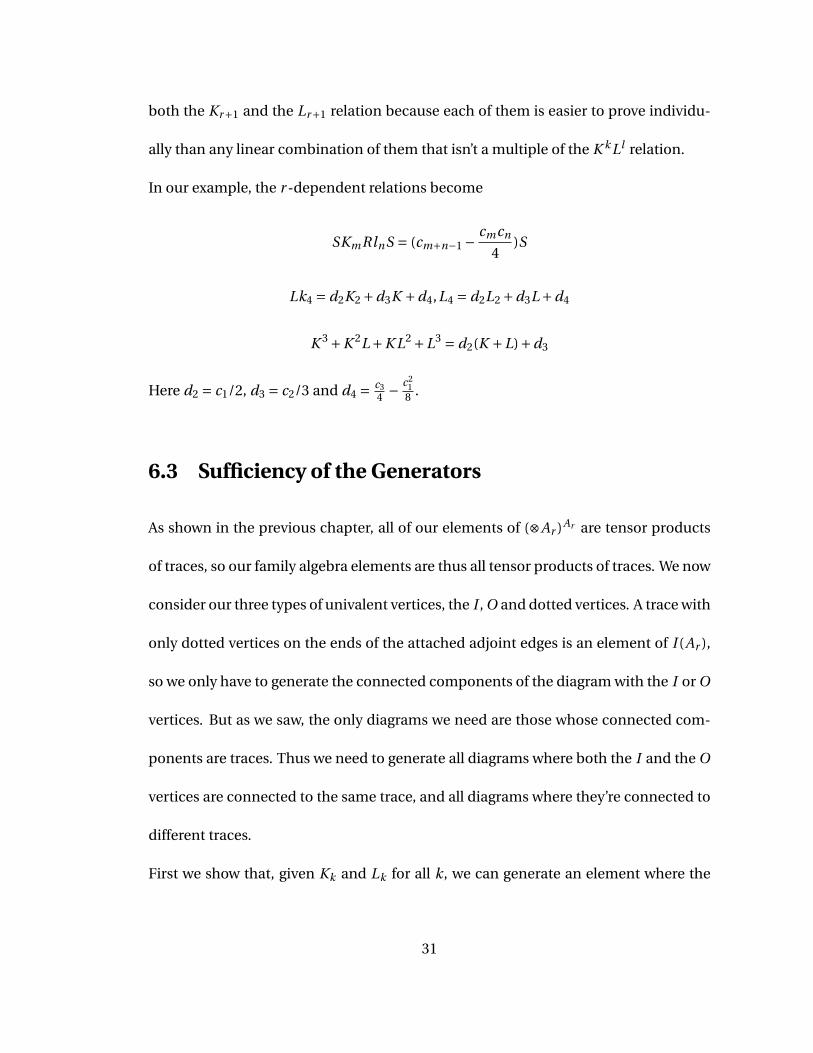
In our example, the r -dependent relations become
SKmRlnS = (cm+n−1 − cmcn
4)S
Lk4 = d2K2 +d3K +d4,L4 = d2L2 +d3L+d4
K 3 +K 2L+K L2 +L3 = d2(K +L)+d3
Here d2 = c1/2, d3 = c2/3 and d4 = c34 − c2
18 .
6.3 Sufficiency of the Generators
As shown in the previous chapter, all of our elements of (⊗Ar )Ar are tensor products
of traces, so our family algebra elements are thus all tensor products of traces. We now
consider our three types of univalent vertices, the I , O and dotted vertices. A trace with
only dotted vertices on the ends of the attached adjoint edges is an element of I (Ar ),
so we only have to generate the connected components of the diagram with the I or O
vertices. But as we saw, the only diagrams we need are those whose connected com-
ponents are traces. Thus we need to generate all diagrams where both the I and the O
vertices are connected to the same trace, and all diagrams where they’re connected to
different traces.
First we show that, given Kk and Lk for all k, we can generate an element where the
31
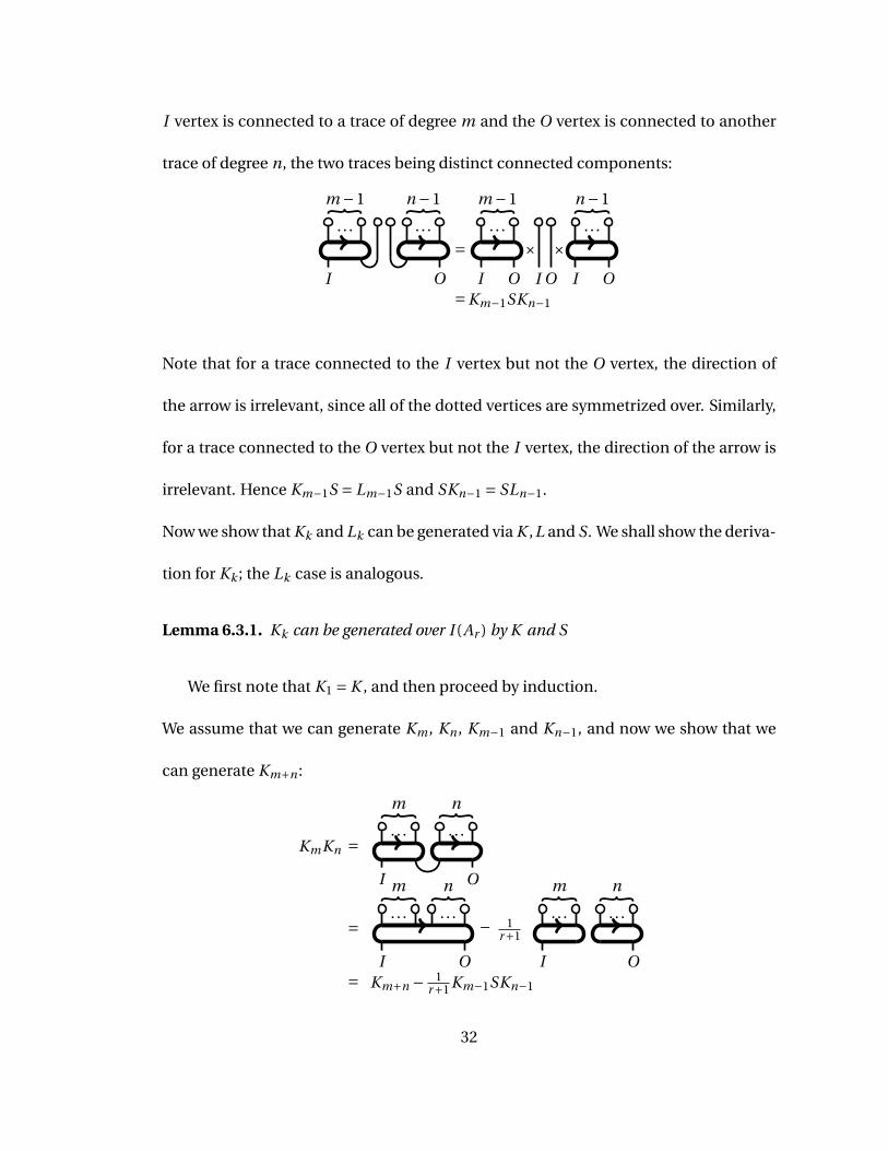
I vertex is connected to a trace of degree m and the O vertex is connected to another
trace of degree n, the two traces being distinct connected components:
I
. . .
m −1
. . .
n −1
O
=I
. . .
m −1
O
×I O
×I
. . .
n −1
O=Km−1SKn−1
Note that for a trace connected to the I vertex but not the O vertex, the direction of
the arrow is irrelevant, since all of the dotted vertices are symmetrized over. Similarly,
for a trace connected to the O vertex but not the I vertex, the direction of the arrow is
irrelevant. Hence Km−1S = Lm−1S and SKn−1 = SLn−1.
Now we show that Kk and Lk can be generated via K ,L and S. We shall show the deriva-
tion for Kk ; the Lk case is analogous.
Lemma 6.3.1. Kk can be generated over I (Ar ) by K and S
We first note that K1 = K , and then proceed by induction.
We assume that we can generate Km , Kn , Km−1 and Kn−1, and now we show that we
can generate Km+n :
KmKn =I
. . .
m
. . .
n
O
=I
. . .
m
. . .
n
O
− 1r+1
I
. . .
m
. . .
n
O= Km+n − 1
r+1 Km−1SKn−1
32
The second line uses the projection from V ⊗V ∨ to the adjoint representation to re-
move the internal adjoint edge. Thus we can write
Km+n = KmKn + 1
r +1Km−1SKn−1
So thus we can generate Kk for all k.
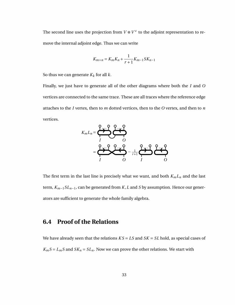
Finally, we just have to generate all of the other diagrams where both the I and O
vertices are connected to the same trace. These are all traces where the reference edge
attaches to the I vertex, then to m dotted vertices, then to the O vertex, and then to n
vertices.
KmLn =I
. . . . . .
O
=I
. . . . . .
O
− 1r+1
I
. . . . . .
O
The first term in the last line is precisely what we want, and both KmLn and the last
term, Km−1SLn−1, can be generated from K ,L and S by assumption. Hence our gener-
ators are sufficient to generate the whole family algebra.
6.4 Proof of the Relations
We have already seen that the relations K S = LS and SK = SL hold, as special cases of
KmS = LmS and SKn = SLn . Now we can prove the other relations. We start with
33
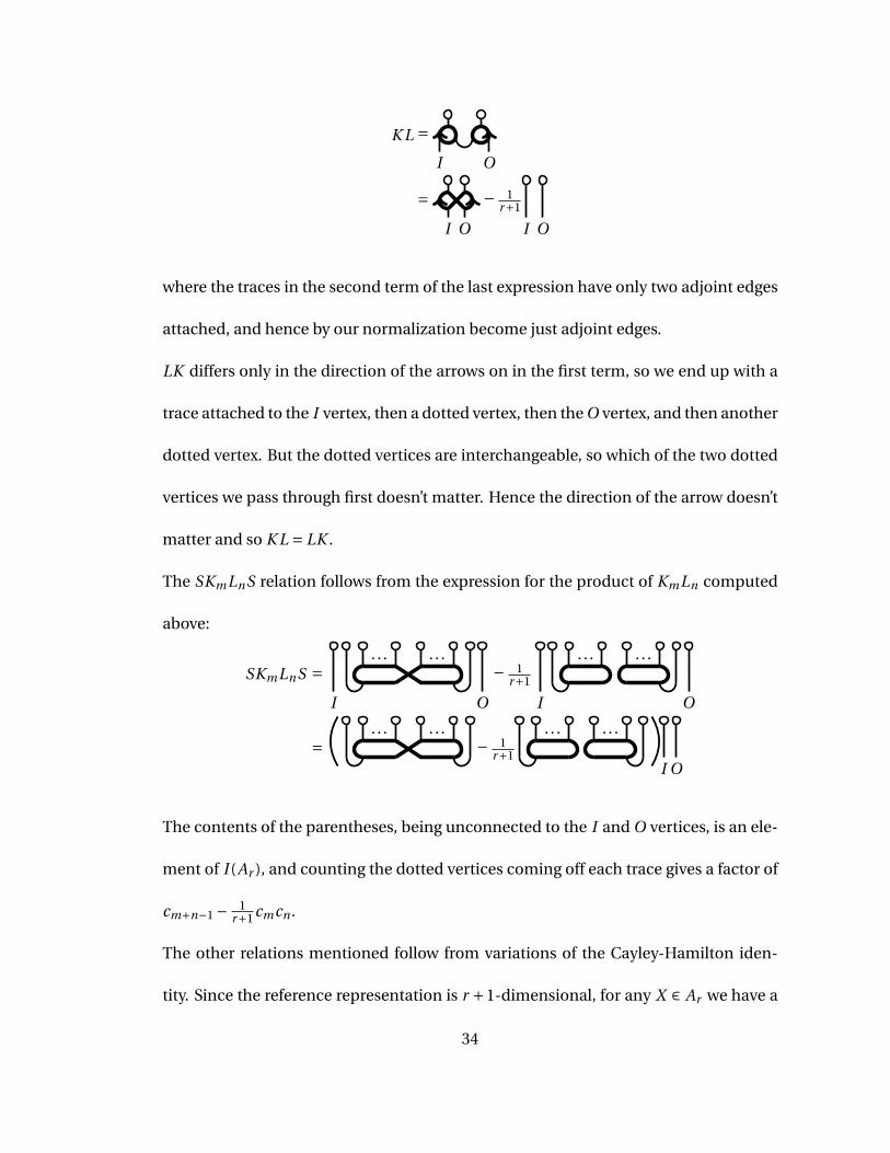
K L =I O
=I O
− 1r+1
I O
where the traces in the second term of the last expression have only two adjoint edges
attached, and hence by our normalization become just adjoint edges.
LK differs only in the direction of the arrows on in the first term, so we end up with a
trace attached to the I vertex, then a dotted vertex, then the O vertex, and then another
dotted vertex. But the dotted vertices are interchangeable, so which of the two dotted
vertices we pass through first doesn’t matter. Hence the direction of the arrow doesn’t
matter and so K L = LK .
The SKmLnS relation follows from the expression for the product of KmLn computed
above:
SKmLnS =I
. . . . . .
O
− 1r+1
I
. . . . . .
O
=. . . . . .
− 1r+1
. . . . . .
I O
The contents of the parentheses, being unconnected to the I and O vertices, is an ele-
ment of I (Ar ), and counting the dotted vertices coming off each trace gives a factor of
cm+n−1 − 1r+1 cmcn .
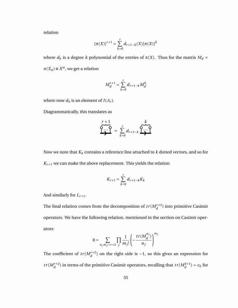
The other relations mentioned follow from variations of the Cayley-Hamilton iden-
tity. Since the reference representation is r +1-dimensional, for any X ∈ Ar we have a
34
relation
[π(X )]r+1 =r∑
k=0dr+1−k (X )[π(X )]k
where dk is a degree k polynomial of the entries of π(X ). Thus for the matrix Md =
π(Xα)⊗Xα, we get a relation
M r+1d =
r∑k=0
dr+1−k M kd
where now dk is an element of I (Ar ).
Diagrammatically, this translates as
. . .
r +1
=r∑
k=0dr+1−k
. . .
k
Now we note that Kk contains a reference line attached to k dotted vectors, and so for
Kr+1 we can make the above replacement. This yields the relation
Kr+1 =r∑
k=0dr+1−k Kk
And similarly for Lr+1.
The final relation comes from the decomposition of tr (M r+2d ) into primitive Casimir
operators. We have the following relation, mentioned in the section on Casimir oper-
ators:
0 = ∑n j m j=r+2
∏j
1
m j !
(− tr (M
n j
d )
n j
)m j
The coefficient of tr (M r+2d ) on the right side is −1, so this gives an expression for
tr (M r+2d ) in terms of the primitive Casimir operators, recalling that tr (M k+1
d ) = ck for
35
1 ≤ k ≤ r .
We can translate this fact into one about the family algebra by writing all of the traces
as diagrammatic traces, connected only to dotted vertices, and then for each diagram
writing out all the ways to replace a dotted vertex by the I vertex and another dotted
vertex by the O vertex. This is equivalent to taking derivatives with respect to the vec-
tors corresponding to the edges connected to the I and O vertices.
Given a trace of degree d with only dotted vertices, there are d ways to replace one
dotted vertex by the I vertex, and all the ways yield the same diagram. Given a product
of traces with only dotted vertices, the number of ways to replace a dotted vertex by
the I vertex is equal to the total degree of the product, with each trace of degree di
yielding di identical diagrams.
Given a trace with the I vertex and d −1 dotted vertices, there are now d −1 ways to
replace a dotted vertex by the O vertex. Given a product of traces with one vertex be-
ing the I vertex and the rest dotted, the number of ways to replace a dotted vertex by
the O vertex is the degree of the product (which only counts the dotted vertices). Note
that we have two possibilities here: the O vertex could be on the same or on a different
trace as the I vertex.
Using the fact that
dk = ∑mi ni=k
∏i
1
mi !
(− tr (Md )ni
ni
)mi
for k ≤ r +1, we get that the sum is thus
0 =∑i , j
dr−i− j−2Ki SL j +∑i , j
dr−i− j Qi , j
36
where Qi , j is a trace connected to the I vertex, then i dotted vertices, then the O vertex,
and then j dotted vertices, which we saw above can be written as
Ki L j + 1
r +1Ki−1SL j−1
Writing out Km and Ln in terms of K ,L and S, we get that all of the terms involving S
automatically cancel out, leaving the relation
r∑k=0
K k Lr−k =r−2∑j=0
dr− j
j∑k=0
K k L j−k
6.5 The Sufficiency of the Relations
Here we show that the relations listed above are sufficient to determine the algebra,
i.e. that any further relations on the algebra can be derived from the relations already
given.
Lemma 6.5.1. No monic polynomial in K +L with coefficients in I (g) and degree less
than r can vanish.
Proof. If we consider K k Lm−k , lower the raised coordinate using the Killing form, and
then symmetrize over all of the indices, coordinate or otherwise, we end up with a
polynomial in Casimir elements of degree m+2 including a term of cm+2 and all other
terms products of Casimir elements of lower degree.
Now suppose that we have a monic polynomial in K +L with coefficients in I (g) and
degree m less than r . Then the leading terms, i.e. the terms involving no nontrivial
37
Casimir elements, has positive coefficients for all terms of the form K k Lm−k and thus
the symmetrization of this polynomial then yields a polynomial in Casimir elements
with nonvanishing cm+2 coefficient.
Since m < r , we have that m+2 < r +2 and hence cm+2 is algebraically independent of
the Casimir elements of lower degree; hence the symmetrization cannot vanish, and
hence the polynomial in (L+R) cannot vanish.
Consider now the K k Ll relation. The leading term is
∑k
K k Lr−k
and hence multiplying this leading term by (K +L)m yields a polynomial in K and L
that only has positive coefficients. In particular, the term K r Lm has positive coeffi-
cient in this polynomial. For m ≤ r , neither K r nor Lm can be reduced by the Kr+1 or
Lr+1 relations.
Hence we get that for m < r , (K +L)m times the K k Ll relation yields a relation in each
degree greater than r − 1 that cannot be deduced from the other relations. Since no
polynomial in K +L vanishes for degree less than r , we get that the relations of the
form (K +L)m times the K k Ll relation are themselves linearly independent from one
another over I (g). We also get a relation in degree 2r by squaring the K k Ll relation,
and this one is also linearly independent from the other relations since the K k Ll rela-
tion is itself a polynomial in K and L that is linearly independent from all polynomials
in K +L, just by comparing leading coefficients.
Now we show that there cannot be any other relations that are not in the ideal gener-
38
ated by the ones listed. We do so by counting the number of I (g)-linearly independent
monomials.
Note that since K S = LS, we can write K r S = 1r+1
∑k
K k Lr−k S. Hence, using the K k Ll
relation, we can reduce Lr S to terms involving nontrivial Casimir elements. Hence we
get that K r SLl is not linearly independent over I (g) from terms of lower degree. Simi-
larly, K k SLr cannot be linearly independent.
Thus we get that our linearly independent monomials are K k SLl for 0 ≤ k, l ≤ r −1 and
K k Ll for 0 ≤ k, l ≤ r , minus one in each degree between r and 2r since (K +L)m times
the K k Ll relation gives K r Lm in terms of other monomials.
This yields a total of 2r 2 + r terms not known to be linearly dependent. If there are
more relations, then there will be fewer linearly independent terms.
The dimension formula for family algebras tells us that we should be getting
di mI (g)Cg(g) = ∑λ∈W t (g)
mg(λ)2
For the adjoint representation, the weights with non-zero multiplicity are the roots,
each with multiplicity 1, and 0, with multiplicity equal to the rank of the algebra. This
gives us r (r + 1)+ r 2 = 2r 2 + r . Hence, since the relations given above limit us to at
most 2r 2 + r linearly independent elements and any further relations would reduce
that number, there cannot be any more relations.
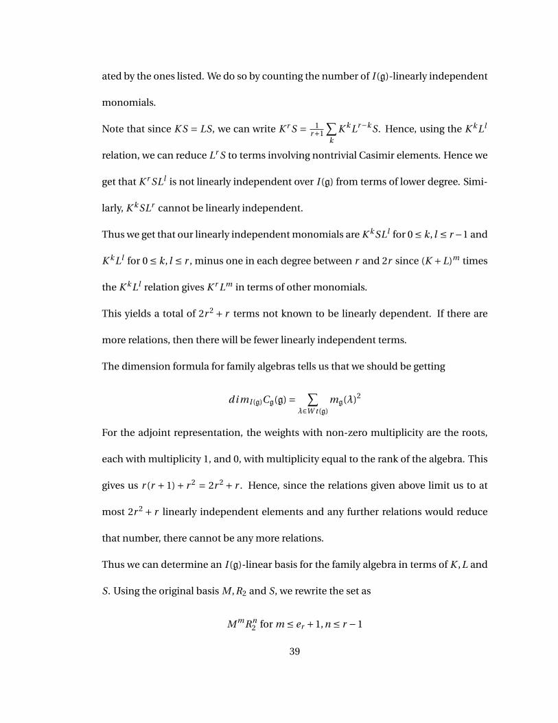
Thus we can determine an I (g)-linear basis for the family algebra in terms of K ,L and
S. Using the original basis M ,R2 and S, we rewrite the set as
M mRn2 for m ≤ er +1,n ≤ r −1
39
Rm2 SRn
2 +Rn2 SRm
2 for m ≤ n ≤ r −2
Rm2 SRn
2 −Rn2 SRm
2 for m < n ≤ r −1
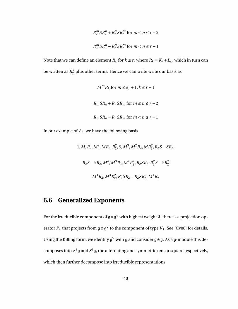
Note that we can define an element Rk for k ≤ r , where Rk = Kr +Lk , which in turn can
be written as Rk2 plus other terms. Hence we can write write our basis as
M mRk for m ≤ er +1,k ≤ r −1
RmSRn +RnSRm for m ≤ n ≤ r −2
RmSRn −RnSRm for m < n ≤ r −1
In our example of A3, we have the following basis
1, M ,R2, M 2, MR2,R22 ,S, M 3, M 2R2, MR2
2 ,R2S +SR2,
R2S −SR2, M 4, M 3R2, M 2R22 ,R2SR2,R2
2S −SR22
M 4R2, M 3R22 ,R2
2SR2 −R2SR22 , M 4R2
2
6.6 Generalized Exponents
For the irreducible component of g⊗g∨ with highest weightλ, there is a projection op-
erator Pλ that projects from g⊗g∨ to the component of type Vλ. See [Cv08] for details.
Using the Killing form, we identify g∨ with g and consider g⊗g. As a g-module this de-
composes into ∧2g and S2g, the alternating and symmetric tensor square respectively,
which then further decompose into irreducible representations.
40
For r = 1, ∧2g is isomorphic to g itself, and hence is the adjoint representation, with
generalized exponent 1. S2g decomposes into a trivial representation and a repre-
sentation of dimension 5; these representations have generalized exponents 0 and 2
respectively.
For r = 2, ∧2g decomposes into a copy g, with generalized exponents 1 and 2, and two
dual 10-dimensional representations with weights 3ω1 and 3ω2 respectively and each
with generalized exponent 3. S2g decomposes into the trivial representation with gen-
eralized exponent 0, another copy of g, again with generalized exponents 1 and 2, and
a 27-dimensional representation with generalized exponents 2,3 and 4. See [Ro01]
for details. Note that Rozhkovskaya uses a different basis, generated by harmonic el-
ements. Her M1 is proportional to M , her N1 is proportional to R2, and her N2 is pro-
portional to 3R22 +3M 2 +S + c1.
For r ≥ 3, the decomposition of g⊗ g is uniform. ∧2g decomposes into a copy of g
and two dual representations with highest weights 2ω1 +ωr−1 and ω2 + 2ωr respec-
tively, while S2g decomposes into the trivial representation, another copy of g, and
two representations with highest weights ω2 +ωr−1 and 2ω1 +2ωr respectively. In an
orthonormal basis for g, the corresponding elements of the family algebra are actually
symmetric or antisymmetric as matrices.
The Lk R l reduction relation gives us a relation ∼ on elements in Vω2+ωr−1 ; applying the
differential operator D =(∂
xα c2
)∂∂xα
gives a relation equivalent to the multiples of the
Lk R l relation times L +R, modulo the Lr+1 and Rr+1 relations. Since D transforms as
41
the trivial representation, D applied to both sides of ∼ again gives a relation between
elements of the Vω2+ωr−1 representation; hence we get that the generalized exponents
of Vω2+ωr−1 plus a copy of {r, . . . ,2r } gives the generalized exponents of V2ω1+2ωr .
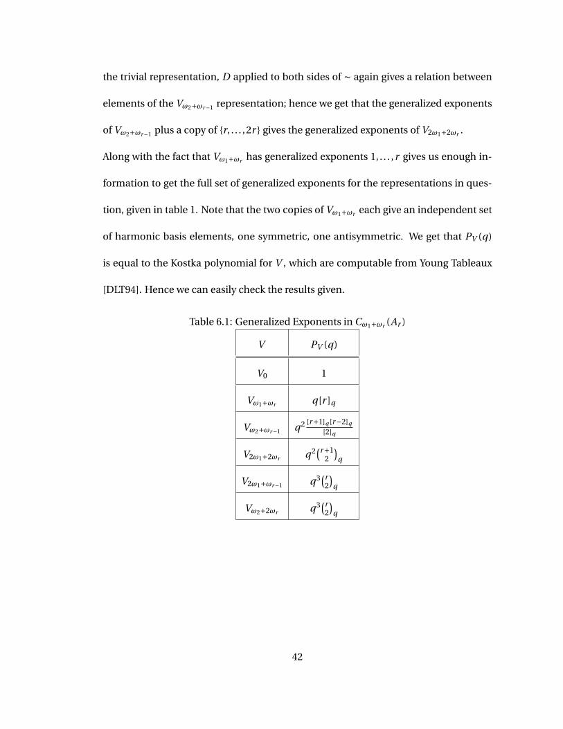
Along with the fact that Vω1+ωr has generalized exponents 1, . . . ,r gives us enough in-
formation to get the full set of generalized exponents for the representations in ques-
tion, given in table 1. Note that the two copies of Vω1+ωr each give an independent set
of harmonic basis elements, one symmetric, one antisymmetric. We get that PV (q)
is equal to the Kostka polynomial for V , which are computable from Young Tableaux
[DLT94]. Hence we can easily check the results given.
Table 6.1: Generalized Exponents in Cω1+ωr (Ar )
V PV (q)
V0 1
Vω1+ωr q[r ]q
Vω2+ωr−1 q2 [r+1]q [r−2]q
[2]q
V2ω1+2ωr q2(r+1
2
)q
V2ω1+ωr−1 q3(r
2
)q
Vω2+2ωr q3(r
2
)q
42
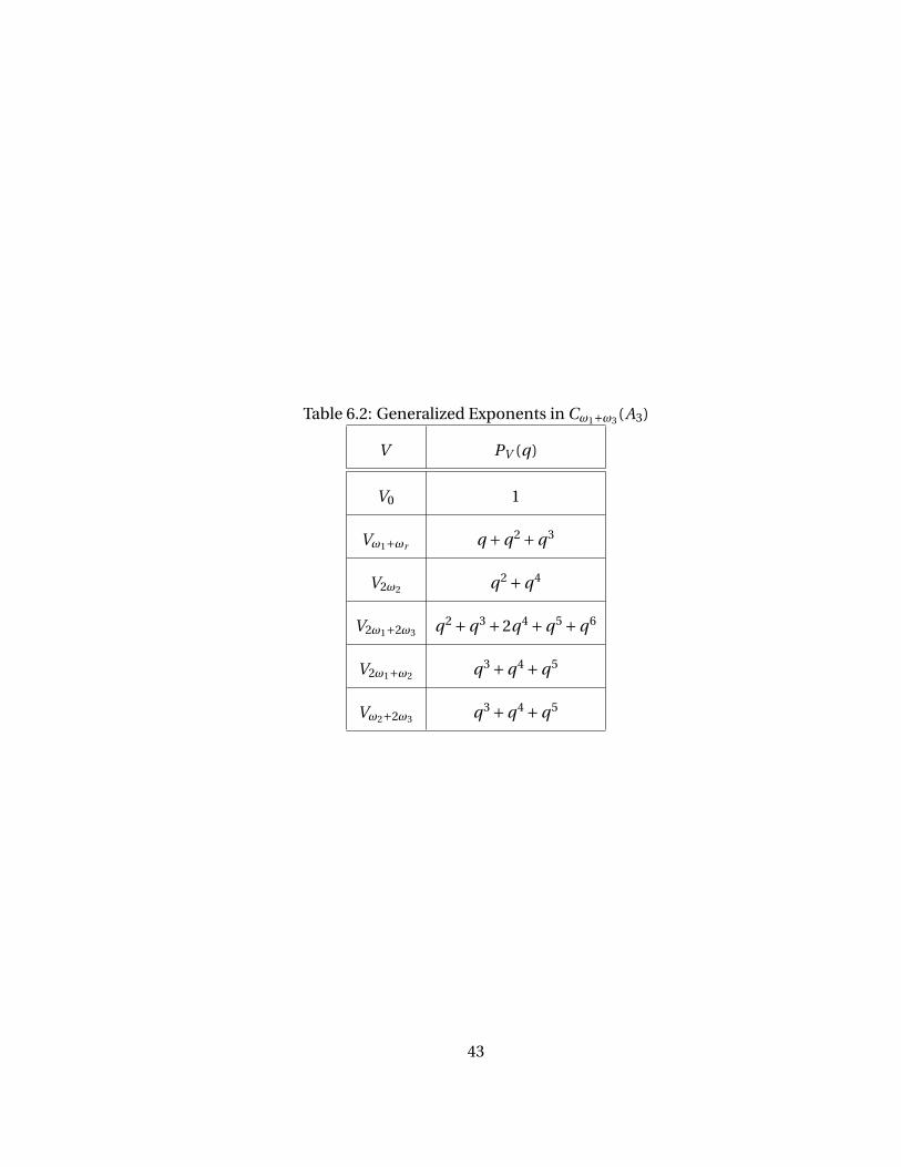
Table 6.2: Generalized Exponents in Cω1+ω3 (A3)
V PV (q)
V0 1
Vω1+ωr q +q2 +q3
V2ω2 q2 +q4
V2ω1+2ω3 q2 +q3 +2q4 +q5 +q6
V2ω1+ω2 q3 +q4 +q5
Vω2+2ω3 q3 +q4 +q5
43
Chapter 7
The Br , Cr case
The cases of Br and Cr end up very similar, so we treat them both here. We start with
Cr since it is somewhat simpler. As with the previous chapter, we use the case of r = 3
as an example.
7.1 Diagrams
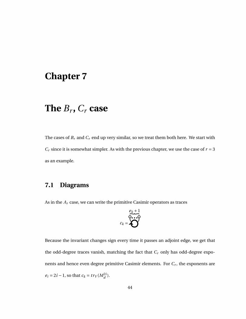
As in the Ar case, we can write the primitive Casimir operators as traces
ck =
ek +1
Because the invariant changes sign every time it passes an adjoint edge, we get that
the odd-degree traces vanish, matching the fact that Cr only has odd-degree expo-
nents and hence even degree primitive Casimir elements. For Cr , the exponents are
ei = 2i −1, so that ck = trV (M 2id ).
44
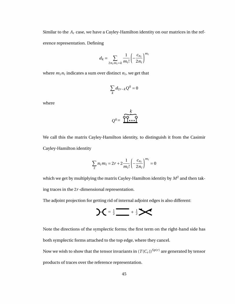
Similar to the Ar case, we have a Cayley-Hamilton identity on our matrices in the ref-
erence representation. Defining
dk = ∑2ni mi=k
1
mi !
(− cni
2ni
)mi
where mi ni indicates a sum over distinct ni , we get that
∑k
d2r−kQk = 0
where
Qk=k
We call this the matrix Cayley-Hamilton identity, to distinguish it from the Casimir
Cayley-Hamilton identity
∑2
ni mi = 2r +21
mi !
(− cni
2ni
)mi
= 0
which we get by multiplying the matrix Cayley-Hamilton identity by M 2 and then tak-
ing traces in the 2r -dimensional representation.
The adjoint projection for getting rid of internal adjoint edges is also different:
= 12 + 1
2
Note the directions of the symplectic forms; the first term on the right-hand side has
both symplectic forms attached to the top edge, where they cancel.
Now we wish to show that the tensor invariants in (T (Cr ))Sp(r ) are generated by tensor
products of traces over the reference representation.
45
All finite dimensional representations of Cr can be written in terms of the reference
representation, so we only have to worry about tensors with adjoint and reference
edges. The vertices are Clebsches between the adjoint and V ⊗V ∨, and the Levi-Civita
tensor on V .
Note that the reference representation, being of dimension 2r , has a Levi-Civita tensor
with 2r vectors coming out of it. Moreover, taking r copies of the symplectic form and
antisymmetrizing all of the edges yields a multiple of the Levi-Civita tensor. Hence the
Levi-Civita tensor can be replaced by the symplectic form. Thus we only have loops
of the reference edges with adjoint edges attached, i.e. traces over the reference repre-
sentation.
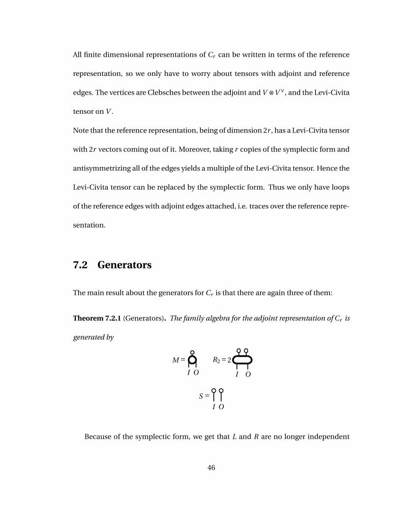
7.2 Generators
The main result about the generators for Cr is that there are again three of them:
Theorem 7.2.1 (Generators). The family algebra for the adjoint representation of Cr is
generated by
M =I O
R2=2
I O
S =I O
Because of the symplectic form, we get that L and R are no longer independent
46
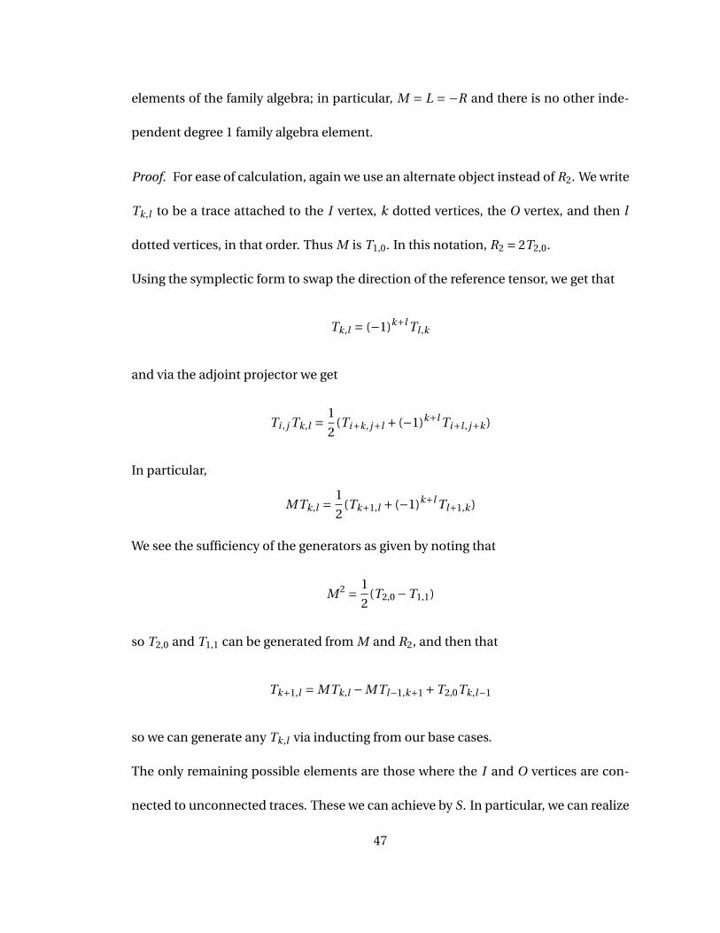
elements of the family algebra; in particular, M = L = −R and there is no other inde-
pendent degree 1 family algebra element.
Proof. For ease of calculation, again we use an alternate object instead of R2. We write
Tk,l to be a trace attached to the I vertex, k dotted vertices, the O vertex, and then l
dotted vertices, in that order. Thus M is T1,0. In this notation, R2 = 2T2,0.
Using the symplectic form to swap the direction of the reference tensor, we get that
Tk,l = (−1)k+l Tl ,k
and via the adjoint projector we get
Ti , j Tk,l =1
2(Ti+k, j+l + (−1)k+l Ti+l , j+k )
In particular,
MTk,l =1
2(Tk+1,l + (−1)k+l Tl+1,k )
We see the sufficiency of the generators as given by noting that
M 2 = 1
2(T2,0 −T1,1)
so T2,0 and T1,1 can be generated from M and R2, and then that
Tk+1,l = MTk,l −MTl−1,k+1 +T2,0Tk,l−1
so we can generate any Tk,l via inducting from our base cases.
The only remaining possible elements are those where the I and O vertices are con-
nected to unconnected traces. These we can achieve by S. In particular, we can realize
47

an element where the I vertex is attached to a trace of degree k and the O vertex to a
trace of degree l by Tk−1,0STl−1,0.
7.3 Relations
Several relations are familiar from the Ar case:
Theorem 7.3.1. The following relations hold for Cr :
SM = MS = 0
R2M = MR2
r∑k=0
d2r−2k T2k,0 = 0
Define
Q2k =2k∑
l=0Tl ,2k−l −
k−1∑l=0
T2l ,0ST2k−2l−2,0
Then
r∑k=0
d2r−2kQ2k = 0
In our example, the r -dependent relations become
−T6,0 +d2T4,0 +d4T2,0 +d6 = 0
2T6,0 +2T5,1 +2T4,2 +T3,3 −T4,0S −T2,0ST2,0 −ST4,0
= d2(2T4,0 +2T3,1 +T2,2 −T2,0S −ST2,0)+d4(2T2,0 +T1,1 −S)+d6
48
The first two relations can be seen by expanding out the relevant diagrams, or in the
case of the second relation by expanding out the Tk,l relations.
For the third relation, we have the matrix Cayley-Hamilton relation, which, as in the Ar
case, gives us a relation on reference edges connected by adjoint edges to only dotted
vertices. For Cr , the identity only involves even powers of the matrix, which translates
to an even number of dotted vertices. T2k,0 involves a reference edge connected to 2k
dotted vertices, and thus we get the third relation.
The fourth relation comes from taking the decomposition of tr (M 2r+2d ) into primitive
Casimir operators, interpreting it as diagrams, and replacing dotted vertices with I and
O vertices, analogous to the LmRn relation for Ar .
Note that the third relation has no mentions of S, and the fourth relation has both
ST2k,0 and T2k,0S. Thus if P times the third relation yields R l2 of the fourth relation, we
get that l = r and thus we get that at the very least the fourth relation yields r relations
that are independent of the third relation.
We now use a counting argument. We can form objects of the forms Ti , j and Tk,0STl ,0.
We note that if k or l is odd, then Tk,0STl ,0 vanishes, due to the symplectic form. So we
really only have Ti , j and T2k,0ST2l ,0. By the third relation, we can limit i + j to be less
than 2r , and we can limit i ≤ j since Ti , j and T j ,i are not independent. We can simi-
larly limit k and l to be less than r . So we have Ti , j for 0 ≤ i ≤ j ≤ 2r −1 and T2k,0ST2l ,0
for 0 ≤ k, l ≤ r −1. This yields a total of 3r 2 + r elements, from which the fourth rela-
tion removes another r elements, to yield 3r 2 linearly independent elements. By the
49
dimension formula for family algebras, we should be getting r 2 +2r 2 = 3r 2 elements.
Since there are no more elements to remove, there are no more relations.
We will thus take as our basis Ti , j for 0 ≤ i ≤ j ≤ 2r − 1, T2k,0ST2l ,0 +T2l ,0ST2k,0 for
k, l ≤ r −2 and T2k,0ST2l ,0 −T2l ,0ST2k,0 for k, l ≤ r −1. To make it more in line with the
results for other Lie algebras, we write this as
M mRn2 for m ≤ er +1,n ≤ r −1
Rm2 SRn
2 +Rn2 SRm
2 for m ≤ n ≤ r −2
Rm2 SRn
2 −Rn2 SRm
2 for m < n ≤ r −1
Note that we can define an element Rk for k ≤ r as the trace that attaches to the I
vertex, ek −2 dotted vertices, and then to the O vertex which in turn can be written as
Rk2 plus other terms. Hence we can write write our basis as
M mRk for m ≤ er +1,k ≤ r −1
RmSRn +RnSRm for m ≤ n ≤ r −2
RmSRn −RnSRm for m < n ≤ r −1
So for C3, the basis is
1, M , M 2,R2,S, M 3, MR2, M 4, M 2R2,R22 ,R2S +SR2,R2S −SR2,
M 5, M 3R2, MR22 , M 6, M 4R2, M 2R2
2 ,R2SR2,R22S −SR2
2 , M 5R2,
M 3R22 , M 6R2, M 4R2
2 ,R22SR2 −R2SR2
2 , M 5R22 , M 6R2
2
Note that the only difference, at least in the labelling, between this and the basis for
the family algebra for A3 is the maximum power of M allowed.
50
7.4 Br
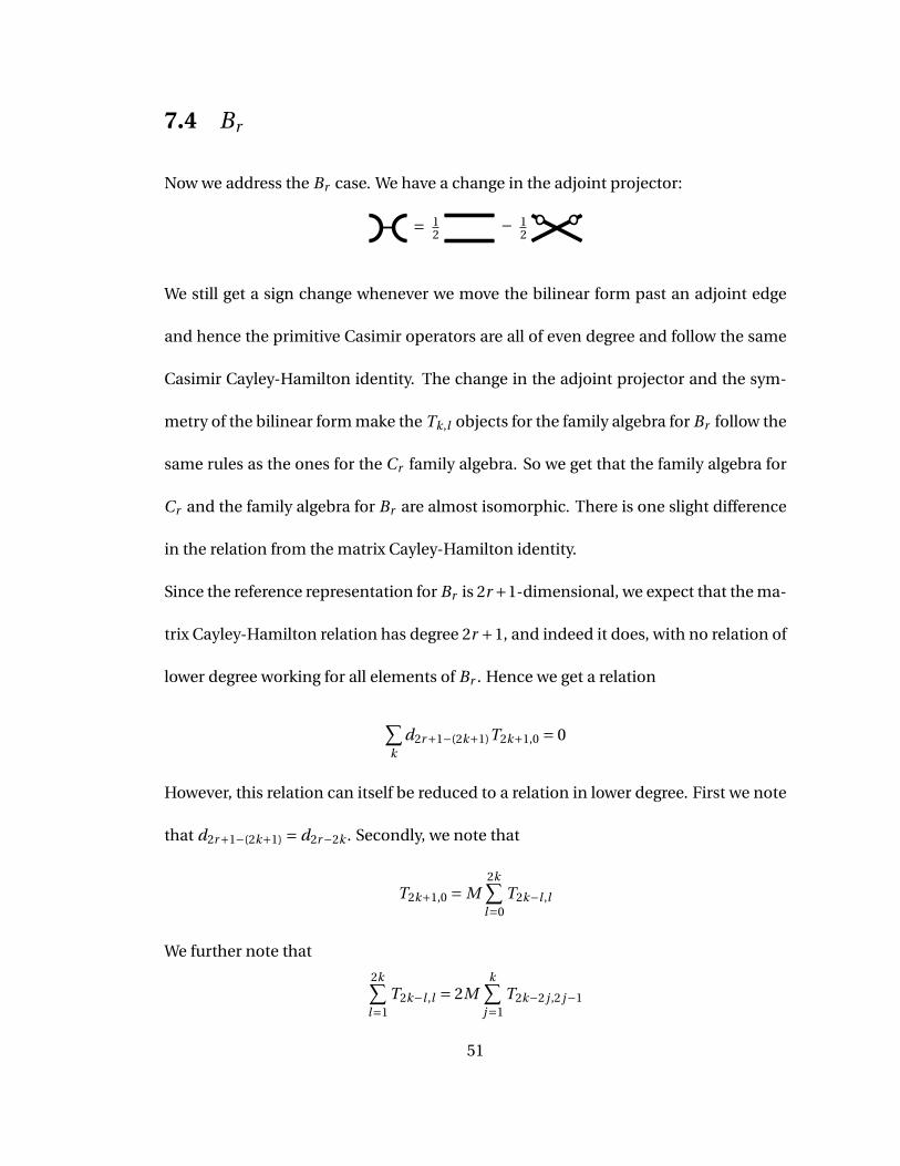
Now we address the Br case. We have a change in the adjoint projector:
= 12
− 12
We still get a sign change whenever we move the bilinear form past an adjoint edge
and hence the primitive Casimir operators are all of even degree and follow the same
Casimir Cayley-Hamilton identity. The change in the adjoint projector and the sym-
metry of the bilinear form make the Tk,l objects for the family algebra for Br follow the
same rules as the ones for the Cr family algebra. So we get that the family algebra for
Cr and the family algebra for Br are almost isomorphic. There is one slight difference
in the relation from the matrix Cayley-Hamilton identity.
Since the reference representation for Br is 2r +1-dimensional, we expect that the ma-
trix Cayley-Hamilton relation has degree 2r +1, and indeed it does, with no relation of
lower degree working for all elements of Br . Hence we get a relation
∑k
d2r+1−(2k+1)T2k+1,0 = 0
However, this relation can itself be reduced to a relation in lower degree. First we note
that d2r+1−(2k+1) = d2r−2k . Secondly, we note that
T2k+1,0 = M2k∑
l=0T2k−l ,l
We further note that
2k∑l=1
T2k−l ,l = 2Mk∑
j=1T2k−2 j ,2 j−1
51
Hence we look at
Q =r∑
k=0d2r−2k
(T2k,0 +2M
k∑j=1
T2k−2 j ,2 j−1
)
Multiplying this by M yields the matrix Cayley-Hamilton relation, i.e. this expression
times M vanishes. Now we look at this object restricted to the Cartan subalgebra.
Since M is invertible on the vector part, since the entry in the xα, xα position is α∨, we
get that since MQ vanishes on the vector part, Q must vanish on the vector part. We
also note that M vanishes on the torus part, so the torus part of Q is
r∑k=0
d2r−2k T2k,0
Since the primitive Casimir operators for Br restricted to the Cartan subalgebra are
identical to the primitive Casimir operators for Cr restricted to the Cartan subalgebra,
we get that sincer∑
k=0d2r−2k T2k,0 vanishes on the torus for Cr , it also must vanish for
Br .
So Q restricted to the Cartan subalgebra must vanish on both the vector and torus
parts, and hence vanishes everywhere. Since the restriction map is an injection, Q it-
self must vanish. Hence we have a relation in degree 2r rather than 2r +1.
Again, this relation involves no terms of S, so again the Casimir Cayley-Hamilton iden-
tity yields r separate relations, and the counting argument above still holds. Hence we
get that the relations for Br are as follows:
Theorem 7.4.1. The following relations hold for Br :
SM = MS = 0
52
R2M = MR2
r∑k=0
d2r−2k
(T2k,0 +2M
k∑j=1
T2k−2 j ,2 j−1
)= 0
Define
Q2k =2k∑
l=0Tl ,2k−l −
k−1∑l=0
T2l ,0ST2k−2l−2,0
Then
r∑k=0
d2r−2kQ2k = 0
Hence the family algebra for Br has the same I (g)-linear basis as the family algebra
for Cr , with the two family algebras differing only in the algebraic relations.
In terms of the example of B3, we have the first r -dependent relation being
−T6,0 −2M(T4,1 +T2,3 +T0,5)+d2T4,0 +2d2M(T2,1 +T0,3)+d4T2,0 +2d4MT0,1 +d6 = 0
and the other r -dependent relation being identical to the case for C3. Similarly, the
basis elements are identical to those for C3.
7.5 Generalized Exponents
The decomposition of the tensor square of the adjoint representation into irreducible
components is very similar for Br and Cr . Both decompose into a symmetric part and
an antisymmetric part, with the symmetric part decomposing into four irreducible
components and the antisymmetric part decomposing into two. See [Cv08] for details
and explicit projection operators.
53
Applying the projection operators to the basis elements computed above, we get that
P2(T2k,0ST2l ,0 +T2l ,0ST2k,0) depends only on k + l , and that P2(Ti , j ) is a linear com-
bination of the P2(T2k,0ST2l ,0 +T2l ,0ST2k,0) terms. So we get that the component cor-
responding to V2 is spanned by P2(T2k,0S + ST2k,0). Note that while there is a rela-
tion involving T2r−2,0S + ST2r−2,0S, that relation occurs in V2 and thus we get that
P2(T2r−2,0S + ST2r−2,0) is linearly-independent from the set of P2(T2k,0S + ST2k,0) for
k < r −1.
Since V2 corresponds to S2V , we get that V2 should have highest generalized exponent
2r and have r generalized exponents. Hence we get that the generalized exponents for
V2 are thus q2[r ]q2 .
P4(T2k+1,2l+1) =−P4(T2k,0ST2l ,0 +T2l ,0ST2k,0)
=− 1
6(T2k,0ST2l ,0 +T2l ,0ST2k,0)− 2
3T2k+1,2l+1
and P4(T2k,2l ) = 0. So V4 has a generalized exponent for each pair k, l such that k, l ≤
r −2. Hence PV4 (q) = q2(r
2
)q2 .
V1 is the trivial representation, and thus has a single generalized exponent of degree
0. So all the rest of the degrees of the symmetric basis elements give generalized expo-
nents for V3. Thus we have that the generalized exponents of V3 are q2[r +1]q2 [r −1]q2 .
The antisymmetric elements yield degrees q[r ]2q2+q4
(r2
)q2 . The adjoint representation
has exponents q[r ]q2 , so we are left with V6 having exponents q3[3]q(r
2
)q2 .
54
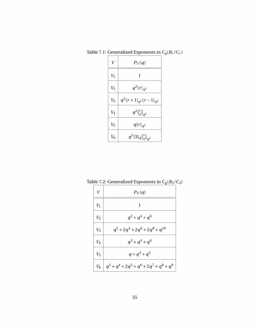
Table 7.1: Generalized Exponents in Cg(Br /Cr )
V PV (q)
V1 1
V2 q2[r ]q2
V3 q2[r +1]q2 [r −1]q2
V4 q2(r
2
)q2
V5 q[r ]q2
V6 q3[3]q(r
2
)q2
Table 7.2: Generalized Exponents in Cg(B3/C3)
V PV (q)
V1 1
V2 q2 +q4 +q6
V3 q2 +2q4 +2q6 +2q8 +q10
V4 q2 +q4 +q6
V5 q +q3 +q5
V6 q3 +q4 +2q5 +q6 +2q7 +q8 +q9
55
Chapter 8
The Dr case
Here we use both r = 3 and r = 4 as examples, as they have somewhat different behav-
ior, and also because r = 3 has already been discussed, via the Ar∼= Dr isomorphism.
8.1 Diagrams
The first fundamental theorem for SO(2r ) acting on the 2r -dimensional representa-
tion tells us that the only invariants are a symmetric bilinear form and a Levi-Civita
tensor. Thus the projection from V ⊗V ∨ to the adjoint representation is the same as
that for Br . Unlike in the Br case, the Levi-Civita tensor has an even number of edges
coming out of it, and so we can have an element of (T (Dr ))SO(2r ) with a single Levi-
Civita tensor in it, and unlike in the Cr case, the Levi-Civita tensor cannot be reduced
to the bilinear form. As a result, the set of primitive Casimir operators for Dr cannot be
expressed solely as traces over the reference representation. Instead, we have traces of
56

2k adjoint edges for 1 ≤ k ≤ r −1, and a degree r Casimir, called the Pfaffian, built from
the Levi-Civita tensor.
P f =
r
Note that since the 2r reference edges going into the Levi-Civita tensor are fully anti-
symmetrized, the adjoint edges attached to the Pfaffian are automatically fully sym-
metrized as a tensor, unlike the traces which have to be symmetrized separately.
We now have a decomposition of tr (M 2rd ) into lower order Casimir operators. We get
∑ni mi=2r
∏i
1
mi !
(− tr (Md )ni
ni
)mi
= 4(−1)r(
P f
r !
)2
The rest of the elements of (T (Dr ))SO(2r ) are either tensor products of traces, or tensor
products of traces with tensors that like the Pfaffian are built from a single Levi-Civita
tensor, only with multiple adjoint edges attached to each reference edge instead of just
one. Note that since the Levi-Civita tensor is fully antisymmetric, the ends of the ref-
erence edges are antisymmetrized, so there must be an odd number of adjoint edges
attached to each one.
8.2 Generators
The generators of Br can be used to generate all of the elements of the family algebra
that do not involve the Pfaffian, but always yield diagrams that only have traces. To get
the diagrams that involve the Pfaffian, we add a fourth generator, P :
57
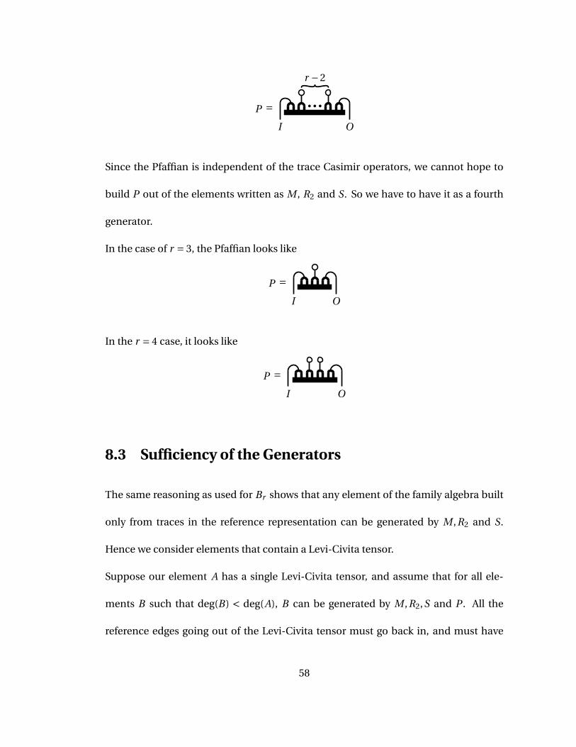
P =I
r −2
O
Since the Pfaffian is independent of the trace Casimir operators, we cannot hope to
build P out of the elements written as M , R2 and S. So we have to have it as a fourth
generator.
In the case of r = 3, the Pfaffian looks like
P =I O
In the r = 4 case, it looks like
P =I O
8.3 Sufficiency of the Generators
The same reasoning as used for Br shows that any element of the family algebra built
only from traces in the reference representation can be generated by M ,R2 and S.
Hence we consider elements that contain a Levi-Civita tensor.
Suppose our element A has a single Levi-Civita tensor, and assume that for all ele-
ments B such that deg(B) < deg(A), B can be generated by M ,R2,S and P . All the
reference edges going out of the Levi-Civita tensor must go back in, and must have
58
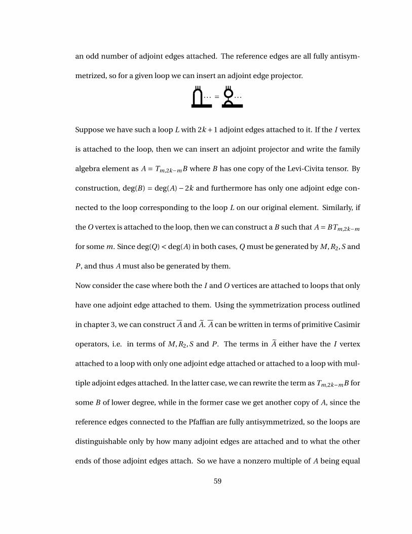
an odd number of adjoint edges attached. The reference edges are all fully antisym-
metrized, so for a given loop we can insert an adjoint edge projector.
. . . = . . .
Suppose we have such a loop L with 2k +1 adjoint edges attached to it. If the I vertex
is attached to the loop, then we can insert an adjoint projector and write the family
algebra element as A = Tm,2k−mB where B has one copy of the Levi-Civita tensor. By
construction, deg(B) = deg(A)− 2k and furthermore has only one adjoint edge con-
nected to the loop corresponding to the loop L on our original element. Similarly, if
the O vertex is attached to the loop, then we can construct a B such that A = BTm,2k−m
for some m. Since deg(Q) < deg(A) in both cases, Q must be generated by M ,R2,S and
P , and thus A must also be generated by them.
Now consider the case where both the I and O vertices are attached to loops that only
have one adjoint edge attached to them. Using the symmetrization process outlined
in chapter 3, we can construct A and A. A can be written in terms of primitive Casimir
operators, i.e. in terms of M ,R2,S and P . The terms in A either have the I vertex
attached to a loop with only one adjoint edge attached or attached to a loop with mul-
tiple adjoint edges attached. In the latter case, we can rewrite the term as Tm,2k−mB for
some B of lower degree, while in the former case we get another copy of A, since the
reference edges connected to the Pfaffian are fully antisymmetrized, so the loops are
distinguishable only by how many adjoint edges are attached and to what the other
ends of those adjoint edges attach. So we have a nonzero multiple of A being equal
59
to something expressible in terms of M ,R2,S and P , plus terms of the form Tm,2k−mB
where B has degree less than A. Since deg(B) < deg(A) for all of the B , they must be
generated by M ,R2,S and P . Thus A must also be generated by them.
Hence M ,R2,S and P generate the entire family algebra.
8.4 Relations
Several of the relations for M ,R2 and S are identical to those from Br :
MR2 = R2M
MS = SM = 0
We have a relation coming from the Cayley-Hamilton identity for Casimir operators:
2PSP +2P f P +r−1∑k=0
d2r−2k−2Q2k = 0
Expanding out Q2k gives us that we can read this relation as expressing Rr−22 S +SRr−2
2
in terms of other elements.
The relation also gives us that Rr−12 S decomposes, since the resulting diagram has a
trace of degree 2r attached to the I vertex but not the O vertex, and thus is it sym-
metrizes to tr (M 2rd ), which decomposes, and all of the diagrams in the symmetriza-
tion are the equal. Similarly, SRr−12 also decomposes.
We also have additional relations involving P :
PS +PT1,1 = 2P f
60
Defining P2k =Q2k −k−1∑l=0
T2l+1,2k−2l−1 for k ≥ 1 and P0 = 1, we get
P 2 + ∑k=0
(−1)r−1d2r−4−2k P2k = 0
So our possibly linearly independent elements are
M mRn2 for m ≤ 2r −2,n ≤ r −2
M mP for m ≤ 2r −2
Rm2 SRn
2 +Rn2 SRm
2 for m ≤ n ≤ r −3
PSRm2 +Rm
2 SP for m ≤ r −3
Rm2 SRn
2 −Rn2 SRm
2 for m < n ≤ r −2
PSRm2 −Rm
2 SP for m ≤ r −2
PSP
Similarly to Ar , Br and Cr , we can define Rk to be an element related to the primitive
Casimir operators, although here we have to be careful about indexing. For k 6= ⌈ r2
⌉, we
define Rk to be the trace that attaches to the I vertex, then to the ek −1 dotted vertices,
and then to the O vertex, while for Rd r2e we use P . Then we can rewrite the basis as
M mRk for m ≤ er +1,k ≤ r −1
RmSRn +RnSRm for m ≤ n ≤ r −2
RmSRn −RnSRm for m < n ≤ r −1
61
This gives a total of 3r 2−2r elements, which matches the number of elements given by
the dimension formula. Note that we could expand PSP by expanding the two Levi-
Civita tensors into antisymmetrized reference edges, but including PSP makes the
full set easier to describe, as well as better matching the list of linearly independent
elements of A3 = D3. In particular, for D3 we have
1, M ,P, M 2, MP,R2,S, M 3, M 2P, MR2,PS +SP,
PS −SP, M 4, M 3P, M 2R2,PSP,R2S −SR2,
M 5, M 4P, M 3R2,PSR2 −R2SP, M 4R2
The P here corresponds to R2 for A3, with R2 here taking the place of R22 for A3. For
r = 4, we have
1, M , M 2,R2,P,S, M 3, MR2, MP,
M 4, M 2R2, M 2P,R22 ,R2S +SR2,PS +SP,
R2S −SR2,PS −SP, M 5, M 3R2, M 3P, MR22 ,
M 6, M 4R2, M 4P, M 2R22 ,R2SR2,PSR2 +R2SP,PSP,
R22S −SR2
2 ,PSR2 −R2SP, M 5R2, M 5P, M 3R22 ,
M 6R2, M 6P, M 4R22 ,R2
2SR2 −R2SR22 ,PSR2
2 −R22SP,
M 5R22 , M 6R2
2
62
8.5 Generalized Exponents
With a few low-dimensional exceptions, for Dr the g⊗g representation decomposes
identically to the Br case: the symmetric subspace of g⊗g decomposes into four irre-
ducible representations, one being the trivial representation, and the antisymmetric
subspace decomposes into two representations, one being the adjoint representation.
The projection operators are identical, except instances of 2r +1 are replaced by 2r . So
we label the six representations P1 through P6, matching the notation from Br . For D3,
the antisymmetric subspace decomposes into three irreducible representations due to
the Pfaffian. This matches the decomposition of A3. For r > 3, the Pfaffian does not
appear in any projection operators, so there six components listed are all irreducible.
The projections of the elements involving only M ,R2 and S are the same as in the Br
case, so we can just examine the elements involving P .
P2(P M 2k ) and P2(PSRk2 ) both decompose into lower order terms. P2(PSP ) can be
written in terms of P2 applied to elements generated by M ,R2 and S. Hence V2 has
generalized exponents PV2 (q) = q2[r −1]q2 , matching the Br case but with [r −1]q2 in-
stead of r due to the decomposition of the degree 2r trace.
P4(P M 2k ) reduces to PSRk2 for k positive, as does P4(PSP ). P4(PSRk
2 ) expands as PSRk2
plus lower order terms. Hence we get that V4 has generalized exponents
PV4 (q) = q2
(r −1
2
)+qr−2[r −1]q2
63
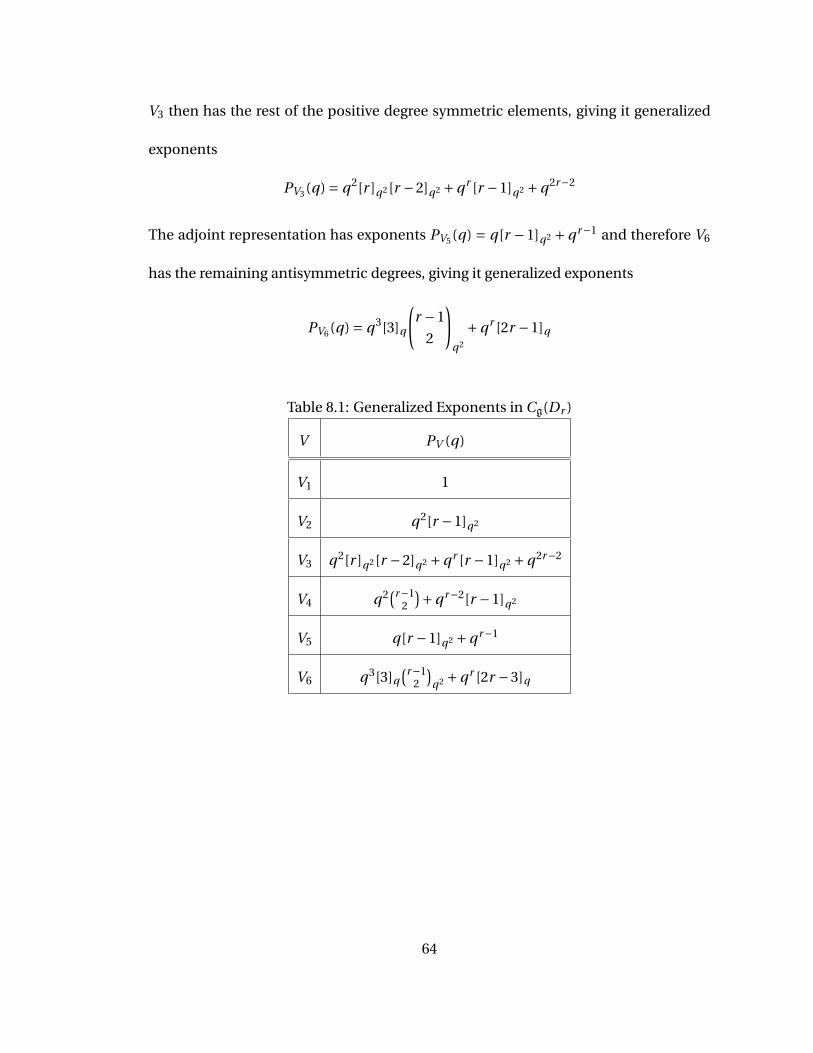
V3 then has the rest of the positive degree symmetric elements, giving it generalized
exponents
PV3 (q) = q2[r ]q2 [r −2]q2 +qr [r −1]q2 +q2r−2
The adjoint representation has exponents PV5 (q) = q[r −1]q2 + qr−1 and therefore V6
has the remaining antisymmetric degrees, giving it generalized exponents
PV6 (q) = q3[3]q
(r −1
2
)q2
+qr [2r −1]q
Table 8.1: Generalized Exponents in Cg(Dr )
V PV (q)
V1 1
V2 q2[r −1]q2
V3 q2[r ]q2 [r −2]q2 +qr [r −1]q2 +q2r−2
V4 q2(r−1
2
)+qr−2[r −1]q2
V5 q[r −1]q2 +qr−1
V6 q3[3]q(r−1
2
)q2 +qr [2r −3]q
64
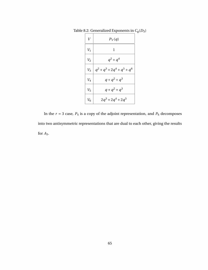
Table 8.2: Generalized Exponents in Cg(D3)
V PV (q)
V1 1
V2 q2 +q4
V3 q2 +q3 +2q4 +q5 +q6
V4 q +q2 +q3
V5 q +q2 +q3
V6 2q3 +2q4 +2q5
In the r = 3 case, P4 is a copy of the adjoint representation, and P6 decomposes
into two antisymmetric representations that are dual to each other, giving the results
for A3.
65
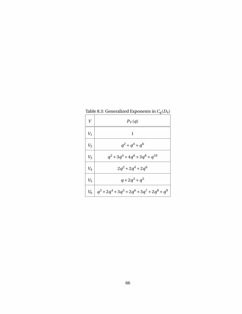
Table 8.3: Generalized Exponents in Cg(D4)
V PV (q)
V1 1
V2 q2 +q4 +q6
V3 q2 +3q4 +4q6 +3q8 +q10
V4 2q2 +2q4 +2q6
V5 q +2q3 +q5
V6 q3 +2q4 +3q5 +2q6 +3q7 +2q8 +q9
66
Chapter 9
Restrictions to Subalgebras
9.1 The Weyl Group Action
The torus part is made of r × r matrices, and as a Weyl-group module is h⊗h. So it
decomposes as 1⊕S2h⊕λ2h, where S2h is the traceless symmetric square of h and λ2h
is the second alternating power. For the non-simply laced algebras Br ,Cr ,G2 and F4
we further divide the vector part into a long part, where the coordinates are long roots,
and a short part, where the coordinates are short roots.
Each part of an h-restricted family algebra element is W -invariant, where W acts on
S(h) in the natural way. Since the coordinates of each part form a representation of W ,
we can find the W -irreducible components of the subspace of g generated by those
coordinates. There is a moduleM(h) such that S(h) ∼= (S(h))W ⊗M(h) andM(h) affords
the regular representation; for an irreducible W -representation U , the fake degrees
67
[Lu77] are the exponents with multiplicity of the polynomial
PU (q) =∑k
dim(HomW (U ,MK (h))qk
and are analogous to generalized exponents for a Lie algebra. They describe the de-
grees of a basis for (BV (h))W , although they do not explicitly give a way to find a basis.
Usually generic degrees are the objects calculated, but fake degrees are computable
from generic degrees [Lu77].
Elements of (BV (h))W can be turned into elements of Cg(g) by either adding elements
on different parts together and trying to adjust for the lack of G-invariance or by mul-
tiplying an element by a G-invariant object whose Cartan restriction vanishes on all
but one part and then extending from h to g.
Here we show how PV (q) for the representations V calculated above can be expressed
in terms of the fake degrees of V T . We use P to denote both generalized exponents of
g representations and fake degrees of W representations. The decomposition of V T
into representations of W can be extracted by setting q = 1, with the labels of P denot-
ing the labels of the representation. For Ar , the subscripts indicate partitions. For BCr
and Dr , the subscripts indicate pairs of partitions (allowing empty partitions or entries
of 0) α and β such that |α|+ |β| = r ; for BCr l (α) = l (β)+1 and for Dr , l (α) = l (β). The
− in φr,− indicates the empty partition.
The decomposition for the exceptional Lie algebras will be discussed in the next chap-
ter.
68
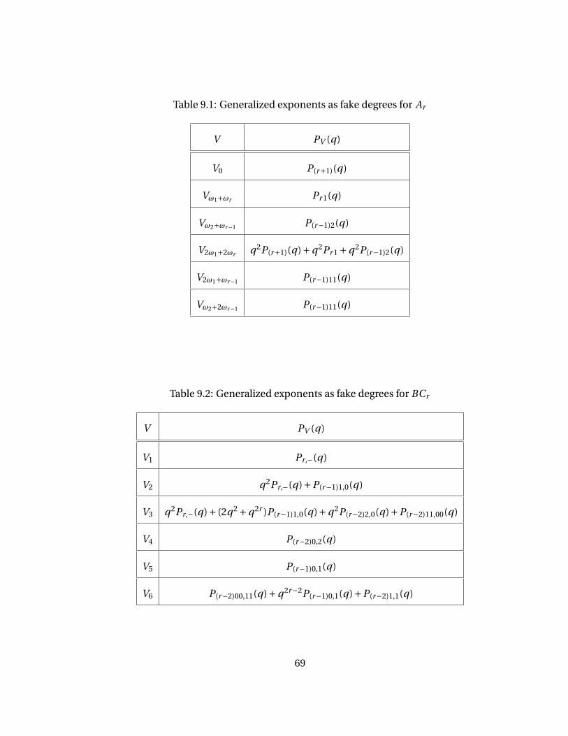
Table 9.1: Generalized exponents as fake degrees for Ar
V PV (q)
V0 P(r+1)(q)
Vω1+ωr Pr 1(q)
Vω2+ωr−1 P(r−1)2(q)
V2ω1+2ωr q2P(r+1)(q)+q2Pr 1 +q2P(r−1)2(q)
V2ω1+ωr−1 P(r−1)11(q)
Vω2+2ωr−1 P(r−1)11(q)
Table 9.2: Generalized exponents as fake degrees for BCr
V PV (q)
V1 Pr,−(q)
V2 q2Pr,−(q)+P(r−1)1,0(q)
V3 q2Pr,−(q)+ (2q2 +q2r )P(r−1)1,0(q)+q2P(r−2)2,0(q)+P(r−2)11,00(q)
V4 P(r−2)0,2(q)
V5 P(r−1)0,1(q)
V6 P(r−2)00,11(q)+q2r−2P(r−1)0,1(q)+P(r−2)1,1(q)
69
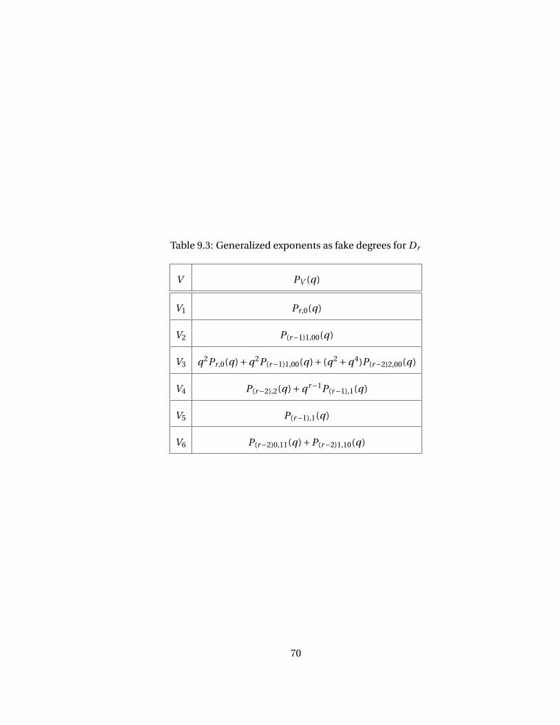
Table 9.3: Generalized exponents as fake degrees for Dr
V PV (q)
V1 Pr,0(q)
V2 P(r−1)1,00(q)
V3 q2Pr,0(q)+q2P(r−1)1,00(q)+ (q2 +q4)P(r−2)2,00(q)
V4 P(r−2),2(q)+qr−1P(r−1),1(q)
V5 P(r−1),1(q)
V6 P(r−2)0,11(q)+P(r−2)1,10(q)
70
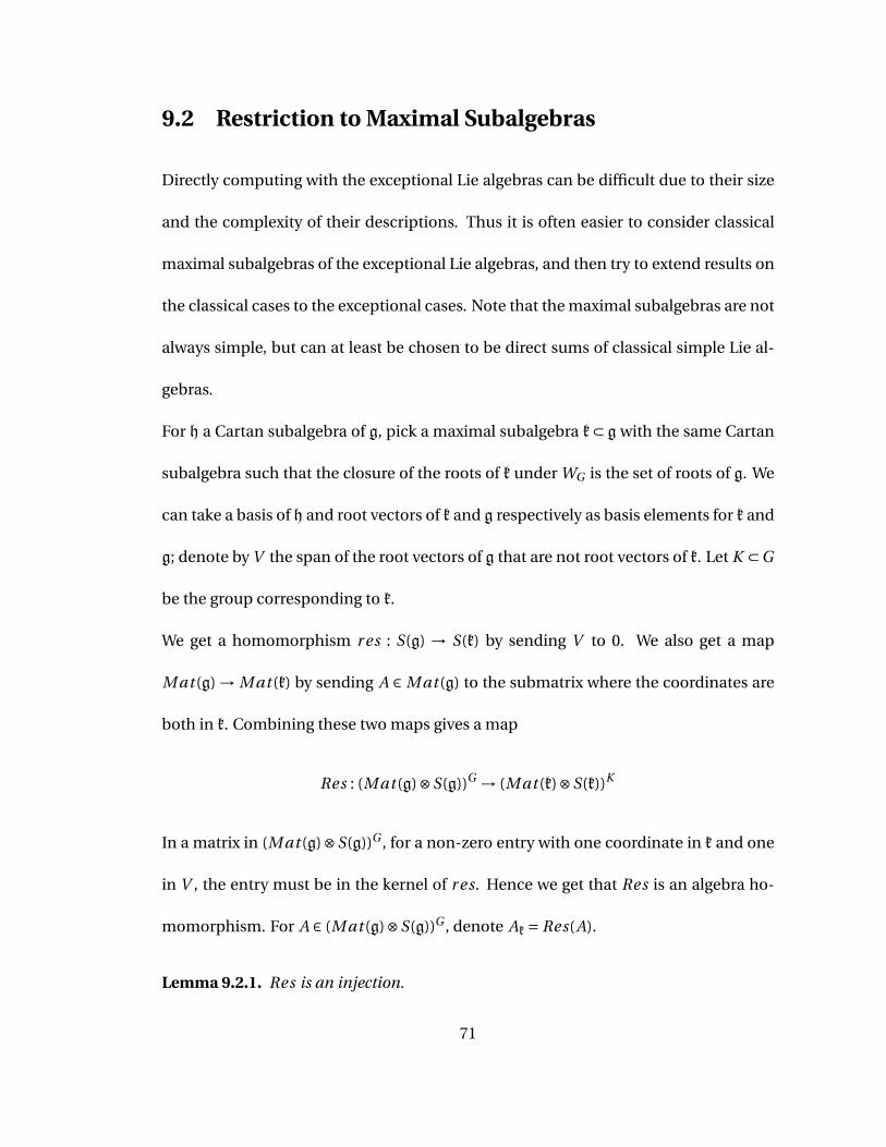
9.2 Restriction to Maximal Subalgebras
Directly computing with the exceptional Lie algebras can be difficult due to their size
and the complexity of their descriptions. Thus it is often easier to consider classical
maximal subalgebras of the exceptional Lie algebras, and then try to extend results on
the classical cases to the exceptional cases. Note that the maximal subalgebras are not
always simple, but can at least be chosen to be direct sums of classical simple Lie al-
gebras.
For h a Cartan subalgebra of g, pick a maximal subalgebra k⊂ g with the same Cartan
subalgebra such that the closure of the roots of k under WG is the set of roots of g. We
can take a basis of h and root vectors of k and g respectively as basis elements for k and
g; denote by V the span of the root vectors of g that are not root vectors of k. Let K ⊂G
be the group corresponding to k.
We get a homomorphism r es : S(g) → S(k) by sending V to 0. We also get a map
M at (g) → M at (k) by sending A ∈ M at (g) to the submatrix where the coordinates are
both in k. Combining these two maps gives a map
Res : (M at (g)⊗S(g))G → (M at (k)⊗S(k))K
In a matrix in (M at (g)⊗S(g))G , for a non-zero entry with one coordinate in k and one
in V , the entry must be in the kernel of r es. Hence we get that Res is an algebra ho-
momorphism. For A ∈ (M at (g)⊗S(g))G , denote Ak = Res(A).
Lemma 9.2.1. Res is an injection.
71
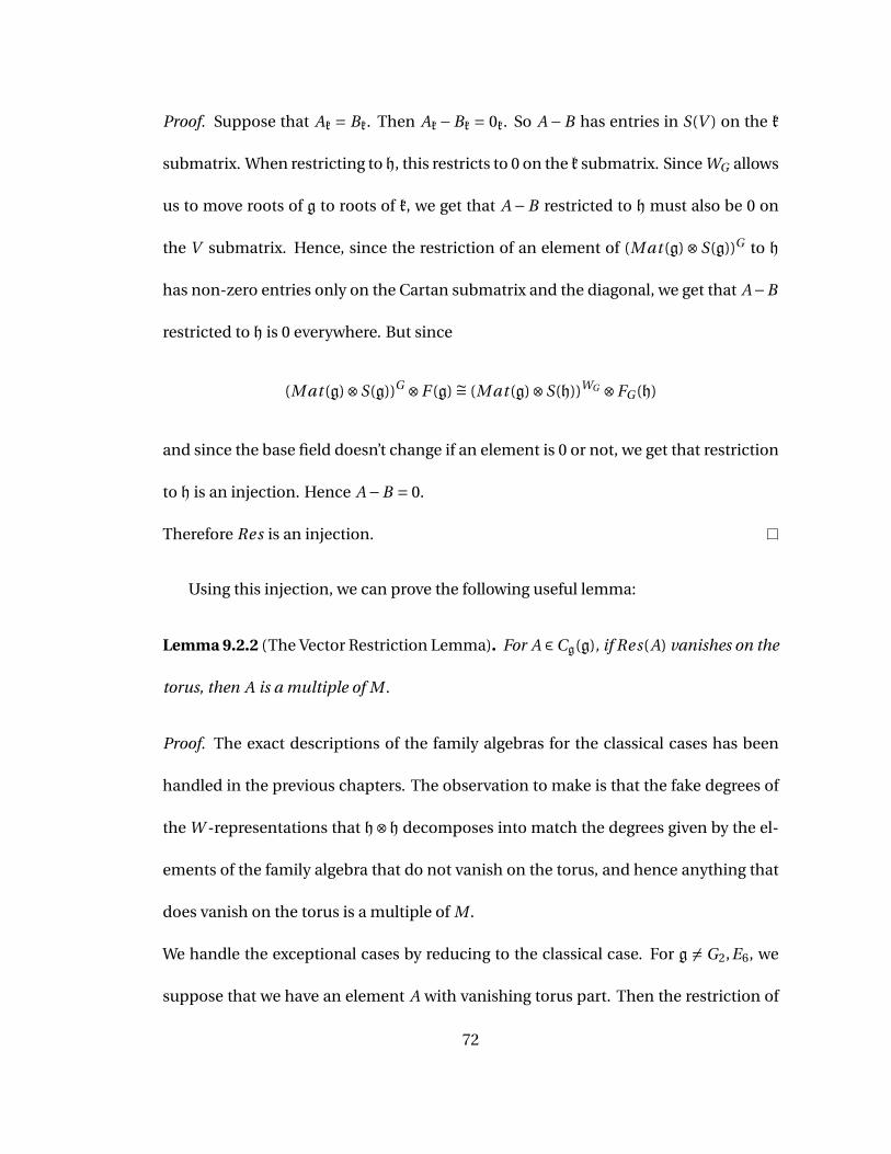
Proof. Suppose that Ak = Bk. Then Ak−Bk = 0k. So A −B has entries in S(V ) on the k
submatrix. When restricting to h, this restricts to 0 on the k submatrix. Since WG allows
us to move roots of g to roots of k, we get that A −B restricted to h must also be 0 on
the V submatrix. Hence, since the restriction of an element of (M at (g)⊗S(g))G to h
has non-zero entries only on the Cartan submatrix and the diagonal, we get that A−B
restricted to h is 0 everywhere. But since
(M at (g)⊗S(g))G ⊗F (g) ∼= (M at (g)⊗S(h))WG ⊗FG (h)
and since the base field doesn’t change if an element is 0 or not, we get that restriction
to h is an injection. Hence A−B = 0.
Therefore Res is an injection.
Using this injection, we can prove the following useful lemma:
Lemma 9.2.2 (The Vector Restriction Lemma). For A ∈Cg(g), if Res(A) vanishes on the
torus, then A is a multiple of M.
Proof. The exact descriptions of the family algebras for the classical cases has been
handled in the previous chapters. The observation to make is that the fake degrees of
the W -representations that h⊗h decomposes into match the degrees given by the el-
ements of the family algebra that do not vanish on the torus, and hence anything that
does vanish on the torus is a multiple of M .
We handle the exceptional cases by reducing to the classical case. For g 6= G2,E6, we
suppose that we have an element A with vanishing torus part. Then the restriction of
72
A to maximal subalgebra k also has vanishing torus part. For F4, we use k= B4, for E7
we use A7 and for E8 we use D8. We look at the part of the vector component of A
that correspond to roots of k. By the first part of the restriction lemma, this part is a
multiple of M restricted to this part and hence can be written as M |kP |k. P |k is W (k)-
invariant, and since both A|k and M |k are invariant under the subgroup of W (g) that
fixes k, P |k is also invariant under that subgroup of W (g) and hence can be extended to
the entire root system of g; we denote the extension by P . Since the extension of M |k
by W (g) is just M , we get that A = MP .
The cases of G2 and E6 have to be handled separately, since E6 has no maximal subal-
gebras that are simple, while G2 has A2 but the image of the roots of A2 under W (G2)
misses some roots of G2. So we consider the case of family algebras for semisimple Lie
algebras.
For a semisimple algebra g⊕k, the adjoint group is GxK where G and K are the adjoint
groups for g and k respectively. For a representation of g⊕k that decomposes as U ⊕V
where g acts trivially on V and k acts trivially on U , we can write the corresponding
family algebra by distributing End(U ⊕V ) and noting that G leaves fixed V , V ∨ and
S(k), and similarly for K :
(End(U ⊕V )⊗S(g⊕ k))G×K =(End(U )⊗S(g))G ⊗ I (k)⊕ (U ⊗S(g))G ⊗ (V v ⊗S(k))K
⊕ (V ⊗S(k))K ⊗ (U∨⊗S(g))G ⊕ (End(V )⊗S(k))K ⊗ I (g)
So we get that the family algebra of U ⊕V breaks into four blocks, depending on if the
coordinates are in U or V . So it remains a free module over I (g⊕ k) = I (g)⊗ I (k).
73
For G2, we use the maximal subalgebra k = k1 ⊕ k2, where k1∼= k2
∼= A1, with one A1
containing a pair of long roots and the other a pair of short roots. The family alge-
bra decomposes into four pieces, as above. For E6, we use the maximal subalgebra
k= k1⊕k2⊕k3, where k1∼= k2
∼= k3∼= A2, and adjoint group K1×K2×K3. We have that the
family algebra of the adjoint representation of k decomposes into nine pieces, three of
which are copies of the family algebra for A2 tensored with two extra copies of S(A2).
Note that for X ∈ ki and Y ∈ k j for i 6= j , the orbit of X under Ki spans ki and thus the
orbit of (X ,Y ) under Ki spans (ki ,Y ).
So suppose that we have an element of Ck(k) which vanishes on the torus. This ele-
ment vanishes on (h1,h2) where h1 and h2 are ki and k j respectively. If i 6= j , then
by the above all entries in (ki ⊗ k∨j ) vanish. If i = j , then we’re in a copy of the family
algebra of mki tensored with S(km)Km ⊗S(kn)Kn for i ,m,n distinct, and thus since the
vector restriction lemma holds for ki , we get that the ki vector part of the family algebra
element thus of the form Mi Pi . Because W (g) intertwines the actions of the ki , we get
that the element that the action of W (g) sends the Pi to each other, and hence Mi Pi
extends to a W (g)-invariant element on the vector part of the family algebra of g, as
was desired.
74

Chapter 10
The Exceptional Lie algebras
10.1 Invariants
The exceptional Lie algebras are not uniform in many senses, so we give a table listing
the data for the reference representation and the exponents:
Table 10.1: Exponents for the Exceptional Lie algebras
g dimV Exponents
G2 7 1,5
F4 26 1,5,7,11
E6 27 1,4,5,7,8,11
E7 56 1,5,7,9,11,13,17
E8 248 1,7,11,13,17,19,23,29
Unlike for the classical Lie algebras, the reference representations of the excep-
75
tional Lie algebras carry invariants of degree higher than 2. For G2, the 7 dimensional
representation has a degree 2 symmetric invariant and a degree 3 antisymmetric in-
variant. For F4, the 26 dimensional representation has a degree 2 symmetric invariant
and a degree 3 symmetric invariant. For E6, the 27 dimensional representation has a
degree 3 symmetric invariant. For E7, the 56 dimensional representation has a degree
2 antisymmetric invariant and a degree 4 symmetric invariant. For E8 the 248 dimen-
sional representation has a degree 2 symmetric invariant and a degree 3 antisymmetric
invariant. The existence of these higher degree invariants gives us elements of (T (g))G
that are not obviously traces over the reference representation.
10.2 The Decomposition of g⊗g
The decomposition of g⊗g into irreducible representations is uniform for the five ex-
ceptional Lie algebras. There are three symmetric representations and two antisym-
metric representations. Of the three symmetric representations, one is the trivial rep-
resentation, and one has highest weight twice that of the adjoint representation, so
we label it S2 Ad j . The remaining symmetric representation we label Sym. Of the
antisymmetric representations, one is the adjoint representation; the other we label
∧2 Ad j .
76
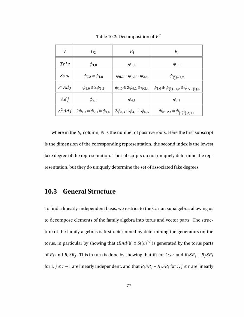
Table 10.2: Decomposition of V T
V G2 F4 Er
Tr i v φ1,0 φ1,0 φ1,0
Sym φ2,2 ⊕φ1,0 φ9,2 ⊕φ1,0 ⊕φ2,4 φ(r2)−1,2
S2 Ad j φ1,0 ⊕2φ2,2 φ1,0 ⊕2φ9,2 ⊕φ2,4 φ1,0 ⊕φ(r2)−1,2 ⊕φN−(r
2),4
Ad j φ2,1 φ4,1 φr,1
∧2 Ad j 2φ1,3 ⊕φ2,1 ⊕φ1,6 2φ8,3 ⊕φ4,1 ⊕φ6,6 φN−r,3 ⊕φ(r−12 ),e2+1
where in the Er column, N is the number of positive roots. Here the first subscript
is the dimension of the corresponding representation, the second index is the lowest
fake degree of the representation. The subscripts do not uniquely determine the rep-
resentation, but they do uniquely determine the set of associated fake degrees.
10.3 General Structure
To find a linearly-independent basis, we restrict to the Cartan subalgebra, allowing us
to decompose elements of the family algebra into torus and vector parts. The struc-
ture of the family algebras is first determined by determining the generators on the
torus, in particular by showing that (End(h)⊗S(h))W is generated by the torus parts
of Ri and Ri SR j . This in turn is done by showing that Ri for i ≤ r and Ri SR j +R j SRi
for i , j ≤ r −1 are linearly independent, and that Ri SR j −R j SRi for i , j ≤ r are linearly
77
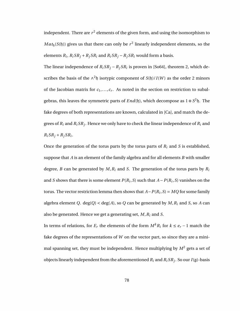
independent. There are r 2 elements of the given form, and using the isomorphism to
M ath(S(h)) gives us that there can only be r 2 linearly independent elements, so the
elements Ri , Ri SR j +R j SRi and Ri SR j −R j SRi would form a basis.
The linear independence of Ri SR j −R j SRi is proven in [So64], theorem 2, which de-
scribes the basis of the ∧2h isotypic component of S(h)/I (W ) as the order 2 minors
of the Jacobian matrix for c1, . . . ,cr . As noted in the section on restriction to subal-
gebras, this leaves the symmetric parts of End(h), which decompose as 1⊕S2h. The
fake degrees of both representations are known, calculated in [Ca], and match the de-
grees of Ri and Ri SR j . Hence we only have to check the linear independence of Ri and
Ri SR j +R j SRi .
Once the generation of the torus parts by the torus parts of Ri and S is established,
suppose that A is an element of the family algebra and for all elements B with smaller
degree, B can be generated by M ,Ri and S. The generation of the torus parts by Ri
and S shows that there is some element P (Ri ,S) such that A−P (Ri ,S) vanishes on the
torus. The vector restriction lemma then shows that A−P (Ri ,S) = MQ for some family
algebra element Q. deg(Q) < deg(A), so Q can be generated by M ,Ri and S, so A can
also be generated. Hence we get a generating set, M ,Ri and S.
In terms of relations, for Er the elements of the form M k Ri for k ≤ er − 1 match the
fake degrees of the representations of W on the vector part, so since they are a mini-
mal spanning set, they must be independent. Hence multiplying by M 2 gets a set of
objects linearly independent from the aforementioned Ri and Ri SR j . So our I (g)-basis
78
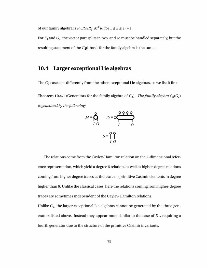
of our family algebra is Ri ,Ri SR j , M k Ri for 1 ≤ k ≤ er +1.
For F4 and G2, the vector part splits in two, and so must be handled separately, but the
resulting statement of the I (g)-basis for the family algebra is the same.
10.4 Larger exceptional Lie algebras
The G2 case acts differently from the other exceptional Lie algebras, so we list it first.
Theorem 10.4.1 (Generators for the family algebra of G2). The family algebra Cg(G2)
is generated by the following:
M =I O
R2=2
I O
S =I O
The relations come from the Cayley-Hamilton relation on the 7-dimensional refer-
ence representation, which yield a degree 6 relation, as well as higher-degree relations
coming from higher degree traces as there are no primitive Casimir elements in degree
higher than 6. Unlike the classical cases, here the relations coming from higher-degree
traces are sometimes independent of the Cayley-Hamilton relations.
Unlike G2, the larger exceptional Lie algebras cannot be generated by the three gen-
erators listed above. Instead they appear more similar to the case of Dr , requiring a
fourth generator due to the structure of the primitive Casimir invariants.
79
Theorem 10.4.2 (Generators for Cg(g) for g = F4,E6,E7,E8). For g = F4,E6,E7 or E8,
Cg(g) is generated over I (g) by
M =I O
R ′2=
. . .e2 −1
I O
+. . .
e2 −1
I O
R ′3=
. . .e3 −1
I O
+. . .
e3 −1
I O
S =I O
While for F4,E7 and E8, the two terms in R ′2 are equal, just as in the G2 case, and
similarly for the two terms in R ′3, for E6 the two terms are different, since the 27-
dimensional reference representation of E6 is not self-dual. Compare this to the Ar
case, for which the reference representation is not self-dual, and contrast with the
Br /Cr and Dr cases, where it is.
For each of them, the elements R ′2 and R ′
3 do not commute, but there are commuting
elements R2 and R3 that can be written as R ′2 plus lower order terms and R ′
3 plus lower
order terms respectively.
As with the other cases, M is central and vanishes on the torus part, S vanishes on
the vector part, and the other relations come from reductions of traces with degrees
that aren’t primitive Casimir operators. In particular, the terms of the form Rm2 Rn
3
are expressible in terms of other elements for m(e2 −1)+n(e3 −1) not equal to ei −1
80
for some i , and Rn2 Rm
3 S +SRm2 Rn
3 is also expressible in terms of other elements when
m(e2 −1)+n(e3 −1) = er −1.
81
Chapter 11
G2
The real compact group associated to G2 is usually defined as the group of automor-
phisms of the octonions O as a division algebra over R; we define G2 to be the com-
plexification of the Lie algebra of this group. Since the real part of O is fixed, we get
an irreducible 7-dimensional representation of the automorphism group, which we
complexify to get an irreducible representation of G2. We use this as the reference rep-
resentation.
The 7-dimensional representation has two primitive invariant forms, a symmetric one
gab corresponding to the norm on the octonions, and an antisymmetric trilinear form
fabc corresponding to the imaginary component of the multiplication. Writing ea for
a basis of the imaginary part ofO, we can write our invariant forms as
eaeb =−gab + fabc g cd ed
82
The torus part of G2 decomposes asφ1,0⊕φ2,2⊕φ1,6, while the vector parts decompose
asφ1,0⊕φ2,2⊕φ2,1⊕φ1,3. φ2,1 has fake degrees q+q5, φ2,2 has fake degrees q2+q6 and
φ1,k has fake degree qk . Note that there are actually several inequivalent representa-
tions denoted by φ1,6, φ2,2 and φ1,3, but they have the same fake degrees so we do not
distinguish between them.
The elements 1,S,R2 and R2S − SR2 are all linearly independent on the torus, and
hence the torus parts of these elements generate the torus parts of all elements of the
family algebra. So now we can determine the linearly independent elements on the
vector part.
By the fake degrees, there is only 1 linearly independent order 4 element when re-
stricted to the short roots, but since we can construct M 4 and R2, there must be some
nonzero element P of the family algebra of order 4 that vanishes on the short roots.
Hence M 4 restricted to the short roots can be written in terms of R2 and lower order
terms. Similarly there must be some element nonzero Q of order 6 that vanishes on
the long roots, and hence M 4 restricted to the long roots can be written in terms of R2
and lower order terms. P is not a multiple of Q.
Using the fact that R22 is not amongst the list of linearly independent torus elements
above, we get that the following must be linearly independent on the short roots:
1, M 2,R2
and the same set is also linearly independent on the long roots. Denote this set {Ai }i
Since the set is linearly independent on the long roots, the set {PAi }i is also linearly in-
83
dependent, and vanishes on the short roots. No linear combination of the Ai vanishes
on the short roots, so the set {Ai ,PAi }i is linearly independent. Since M 2 is nonzero
on both the short and long roots, {M 2 Ai , M 2PAi }i are linearly independent, and are
themselves linearly independent from the set of linearly independent torus elements
above, since they all have vanishing torus part. Hence we have all of the linearly inde-
pendent symmetric pieces.
An I (G2) basis of the family algebra can be written as
M mRn2 for 0 ≤ m ≤ 6,n = 0,1
S
R2S −SR2
Considering R1 as a scalar, we get
M mRn for 0 ≤ m ≤ e2,n ≤ 2
RmSRn +RnSRm for 1 ≤ m ≤ n ≤ 1
RmSRn −RnSRm for 1 ≤ m < n ≤ 2
The generalized exponents for the representations in question have already been com-
puted by Pieter Mostert [Mo12] and we can compare them to both the basis above and
the fake degrees.
84
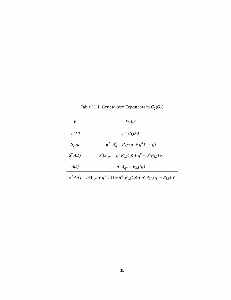
Table 11.1: Generalized Exponents in Cg(G2)
V PV (q)
Tr i v 1 = P1,0(q)
Sym q2[3]2q = P2,2(q)+q4P1,0(q)
S2 Ad j q2[5]q2 = q2P1,0(q)+q2 +q4P2,2(q)
Ad j q[2]q4 = P2,1(q)
∧2 Ad j q[4]q2 +q6 = (1+q4)P1,3(q)+q4P2,1(q)+P1,6(q)
85
Chapter 12
F4
F4 can be thought of as the Lie algebra of the isometry group of the octonionic pro-
jective plane, or as the Lie algebra of the automorphism group of traceless part of
the Albert algebra. It has a symmetric bilinear form and a symmetric trilinear form,
both from the multiplication in the Albert algebra: using e1, . . . ,e26 as the basis of
the traceless part of the Algebra algebra, for v = v aea and w = w beb we get v◦ =
gab v a w b I3 +dabc g cd v a w bed , where I3 is the 3x3-identity matrix.
Alternatively, we view F4 as B4 ⊕∆, where ∆ is the spinor representation of B4 with Lie
bracket given by [X , s] = X .s for X ∈ B4 and s ∈∆, and [s, t ] is defined by ⟨X , [s, t ]⟩B4 =
−⟨X .t , s⟩∆. In this setup, the 26-dimensional representation decomposes as C⊕V9⊕∆
where V9 is the standard 9-dimensional representation of B4; here B4 acts on each
component via the usual representation, while for s ∈ ∆, s.a = as for a ∈ C, s.v = v(s)
for v ∈ V9 where the right-hand side is the usual action of V9 on ∆, and then for t ∈∆,
86
s.t is defined by ⟨u, s.t⟩V9 =−⟨u.t , s⟩∆.
To describe the trilinear form, it is easiest to view everything in terms of so(8) repre-
sentations, with∆ decomposing as∆+ and∆−. the two spinor representations of so(8),
and V9 as V8⊕C. We now get that the 26-dimensional representation can be described
as S ⊕V1 ⊕V2 ⊕V3, where V1 = V8, V2 = ∆+, V3 = ∆−, and S is the subspace of C3 such
that s1 + s2 + s3 = 0 for (s1, s2, s3) ∈ S.
The bilinear form on S is given by (s, t ) = 12 (s1t1 + s2t2 + s3t3), and so the bilinear form
on the 26-dimensional representation is the sum of the bilinear forms on each part.
The trilinear form becomes
(v1, v2, v3) = f (v1, v2, v3) for v1 ∈V1, v2 ∈V2, v3 ∈V3
(s,u, v) = si (u, v) for u, v ∈Vi
(r, s, t ) =−(r1s1t1 + r2s2t2 + r3s3t3) for r, s, t ∈ S
where f is the triality map from V8⊗∆+⊕∆− toC, with the scaling such that | f (x, y, z)| ≤
1 when ‖x‖ = ‖y‖ = ‖z‖ = 1 and the bound is attained for some triple.
with permutations of the arguments above giving the same values and all other triples
of arguments giving 0.
The presence of the bilinear form gives us that all odd degree Casimir operators van-
ish, while the cubic invariant gives us that the quartic and degree 10 Casimir operators
reduce. We are left with exponents of 1,5,7, and 11, giving us primitive Casimir opera-
tors of degrees 2, 6, 8 and 12.
87
Because F4 is not simply laced, there are two root lengths, long and short, so the vec-
tor part of the family algebra decomposes into a long root part and a short root part.
Hence we have three parts. Following [Ca], we write the W -representations as φa,b
where a is the dimension and b is the lowest fake degree. Writing the fake degrees
as exponents of q-multiplicities Qa,b , the torus decomposes as φ1,0 ⊕φ9,2 ⊕φ6,6. The
vector parts each decompose as φ1,0 ⊕φ9,2 ⊕φ2,4 ⊕φ4,1 ⊕φ8,3. Note that the φ2,4 and
φ8,3 labels actually each denote two inequivalent representations, but although the
φ2,4 of the long roots is not equivalent to the φ2,4 of the short roots, the fake degrees
are the same, and similarly for the φ8,3 representations, so the distinction is ignored
here. Also note that except for the trivial and the adjoint representation, none of these
W (F4) representations correspond nicely to representations of F4 itself. They do pro-
vide an upper-limit for the number of linearly-independent elements we can have in
each degree, though. See Table 12.1 for the fake degrees of these representations.
R3 is of degree 6 and hence cannot be generated by M ,S and R2. Hence we need four
generators. R ′2R ′
3−R ′3R ′
2 has degree 10, butφ6,6 has no fake degree of 10, so R ′2R ′
3−R ′3R ′
2
must be reducible to lower order terms. Hence we can define an R2 and an R3 of de-
grees 3 and 4 respectively that commute and that, along with M and S, generate R ′2
and R ′3.
The torus parts of the set Ri for i ≤ 4, Ri SR j +R j SRi for i ≤ j ≤ 3 and Ri SR j −R j SRi
for i < j ≤ 4 form a basis of the torus parts of the algebra, as expected in the general
strategy. Now we determine the linearly independent elements on the vector part.
88
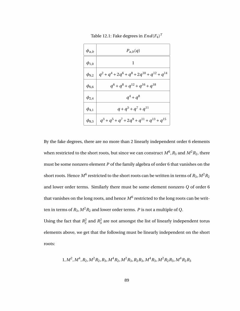
Table 12.1: Fake degrees in End(F4)T
φa,b Pa,b(q)
φ1,0 1
φ9,2 q2 +q4 +2q6 +q8 +2q10 +q12 +q14
φ6,6 q6 +q8 +q12 +q16 +q18
φ2,4 q4 +q8
φ4,1 q +q5 +q7 +q11
φ8,3 q3 +q5 +q7 +2q9 +q11 +q13 +q15
By the fake degrees, there are no more than 2 linearly independent order 6 elements
when restricted to the short roots, but since we can construct M 6,R3 and M 2R2, there
must be some nonzero element P of the family algebra of order 6 that vanishes on the
short roots. Hence M 6 restricted to the short roots can be written in terms of R3, M 2R2
and lower order terms. Similarly there must be some element nonzero Q of order 6
that vanishes on the long roots, and hence M 6 restricted to the long roots can be writ-
ten in terms of R3, M 2R2 and lower order terms. P is not a multiple of Q.
Using the fact that R22 and R2
3 are not amongst the list of linearly independent torus
elements above, we get that the following must be linearly independent on the short
roots:
1, M 2, M 4,R2, M 2R2,R3, M 4R2, M 2R3,R2R3, M 4R3, M 2R2R3, M 4R2R3
89
and the same set is also linearly independent on the long roots. Denote this set {Ai }i
Since the set is linearly independent on the long roots, the set {PAi }i is also linearly in-
dependent, and vanishes on the short roots. No linear combination of the Ai vanishes
on the short roots, so the set {Ai ,PAi }i is linearly independent. Since M 2 is nonzero
on both the short and long roots, {M 2 Ai , M 2PAi }i are linearly independent, and are
themselves linearly independent from the set of linearly independent torus elements
above, since they all have vanishing torus part. Hence we have all of the linearly inde-
pendent symmetric pieces.
The symmetric representations, Tr i v,Sym and S2 Ad j , have 0-weight multiplicities
1, 12 and 21 respectively. Unfortunately, the elements corresponding to parts of the
W (F4) representation do not at all match those corresponding to the various represen-
tations of F4 since the decomposition into torus and vector parts is not F4-invariant.
Hence the determination of which degrees give generalized exponents for which rep-
resentation is nontrivial despite knowing the decompositions of the 0-weight spaces
of the F4-representations into W (F4)-representations.
To determine the generalized exponents of the symmetric representations we exam-
ine the family algebra of the reference representation V of F4. V ⊗V decomposes as
Tr i v⊕V ⊕Sym⊕Ad j ⊕As ym, where As ym is a 273-dimensional representation. The
first three representations belong to S2V , the latter two to ∧2V .
The family algebra CV (F4), restricted to the maximal torus, splits into a 2×2 matrix cor-
responding to the 0-weight space of V and a set of 1×1 matrix algebras corresponding
90
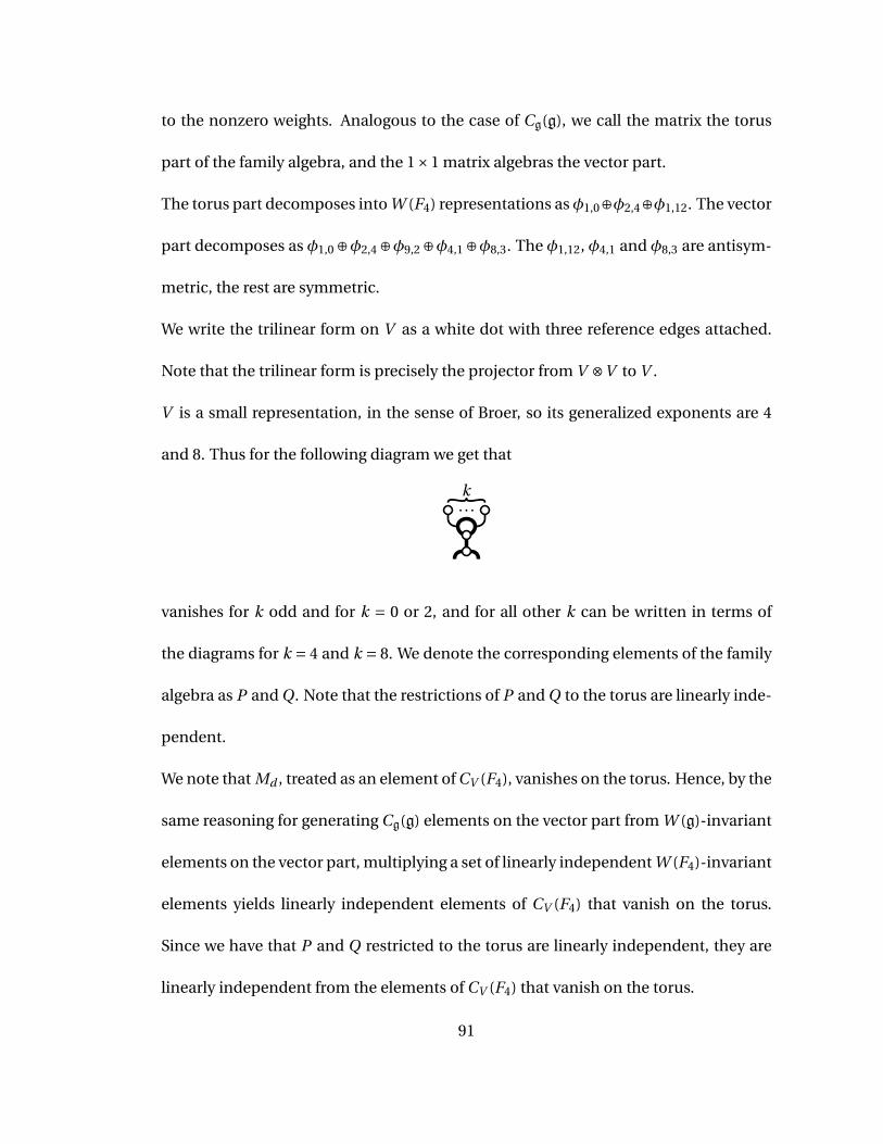
to the nonzero weights. Analogous to the case of Cg(g), we call the matrix the torus
part of the family algebra, and the 1×1 matrix algebras the vector part.
The torus part decomposes into W (F4) representations asφ1,0⊕φ2,4⊕φ1,12. The vector
part decomposes as φ1,0 ⊕φ2,4 ⊕φ9,2 ⊕φ4,1 ⊕φ8,3. The φ1,12, φ4,1 and φ8,3 are antisym-
metric, the rest are symmetric.
We write the trilinear form on V as a white dot with three reference edges attached.
Note that the trilinear form is precisely the projector from V ⊗V to V .
V is a small representation, in the sense of Broer, so its generalized exponents are 4
and 8. Thus for the following diagram we get that
. . .k
vanishes for k odd and for k = 0 or 2, and for all other k can be written in terms of
the diagrams for k = 4 and k = 8. We denote the corresponding elements of the family
algebra as P and Q. Note that the restrictions of P and Q to the torus are linearly inde-
pendent.
We note that Md , treated as an element of CV (F4), vanishes on the torus. Hence, by the
same reasoning for generating Cg(g) elements on the vector part from W (g)-invariant
elements on the vector part, multiplying a set of linearly independent W (F4)-invariant
elements yields linearly independent elements of CV (F4) that vanish on the torus.
Since we have that P and Q restricted to the torus are linearly independent, they are
linearly independent from the elements of CV (F4) that vanish on the torus.
91
Hence the generalized exponents of the symmetric parts of CV (F4) are
(1+q2)P1,0 + (1+q2)P2,4 +q2P9,2
Since we have that q0 is the generalized exponent for the trivial representation and
P2,4 gives the generalized exponents for V , we get that the generalized exponents for
Sym are q2P1,0 +q2P2,4 +q2P9,2.
Returning to the case of Cg(F4), we can now determine the generalized exponents of
S2 Ad j by elimination. We get
PTr i v (q) = q0
PSym(q) = q2P1,0 +q2P2,4 +q2P9,2
PS2 Ad j (q) = q8P1,0 +q8P2,4 + (1+q8)P9,2
We can rewrite the last two expressions as
PSym(q) = P9,2 +q8P1,0 +q8P2,4
PS2 Ad j (q) = q2P1,0 +q2P2,4 + (q2 +q8)P9,2
to better match the results for the other exceptional Lie algebras.
The antisymmetric basis elements are the ones that come from ∧2h or that vanish
on the torus. As with the symmetric elements, we get that {M Ai , MPAi }i are linearly
independent, and this in turn gives us that the M 2k+1, M 2k+1R2, M 2k+1R3 and M 2k+1R4
are linearly independent for k ≤ 5.
92
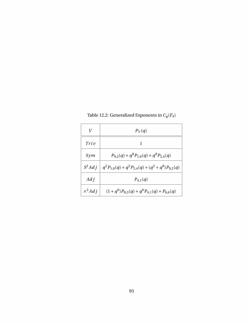
Table 12.2: Generalized Exponents in Cg(F4)
V PV (q)
Tr i v 1
Sym P9,2(q)+q8P1,0(q)+q8P2,4(q)
S2 Ad j q2P1,0(q)+q2P2,4(q)+ (q2 +q8)P9,2(q)
Ad j P4,1(q)
∧2 Ad j (1+q6)P8,3(q)+q6P4,1(q)+P6,6(q)
93
Chapter 13
E6
The reference representation of E6 is 27-dimensional, bearing a symmetric trilinear
form derived from the multiplication on the Albert algebra. Using e1, . . . ,e26 to denote
the 26 traceless basis elements, we write e0 for the identity element and extend dabc by
d0ab = gab for a,b 6= 0, and d00a = 0. E6 is then the group that preserves this extended
dabc without regard to preserving gab .
Alternatively, we can write E6 as a module over (A2)3. We take (A2)1, (A2)2 and (A2)3 to
be three copies of A2, with standard representations U1,U2 and U3. Then
E6 = (A2)1 ⊕ (A2)2 ⊕ (A2)3 ⊕U1 ⊗U2 ⊗U3 ⊕U∨1 ⊗U∨
2 ⊗U∨3
The bracket of an element of one of the (A2)i with something in either U1 ⊗U2 ⊗U3 or
U∨1 ⊗U∨
2 ⊗U∨3 is given by the usual action of (A2)i on Ui or U∨
i . We write
[u1 ⊗u2 ⊗u3, v∨1 ⊗ v∨
2 ⊗ v∨3 ] =∑
i(ui ⊗ v∨
i − tr (ui ⊗ v∨i ))v∨
j (u j )v∨k (uk )
94
where i , j and k cycle through 1,2,3.
The 27-dimensional representation of E6 then becomes U1 ⊗U∨2 ⊕U2 ⊗U∨
3 ⊕U3 ⊗U∨1 .
The action of the three copies of A2 is the usual action. Define a pair of maps φ :
U∨i ⊗U∨
i → Ui and φ∨ : Ui ⊗Ui → U∨i via the determinant on Ui . Then the action of
U1 ⊗U2 ⊗U3 on Ui ⊗U∨j is given by
u1 ⊗u2 ⊗u3.vi ⊗ v∨j = v∨
j (u j )uk ⊗φ∨(ui , vi )
And similarly for U∨1 ⊗U∨
2 ⊗U∨3 ,
u∨1 ⊗u∨
2 ⊗u∨3 .vi ⊗ v∨
j = u∨i (vi )φ(u∨
j , v∨j )⊗u∨
k
The trilinear form now looks like
(u1 ⊗u∨2 , v2 ⊗ v∨
3 , w3 ⊗w∨1 ) = u∨
2 (v2)v∨3 (w3)w∨
1 (u1)
with all permutations of the three arguments giving the same value, and all other
triples of arguments giving 0.
The lack of a bilinear form allows for odd-degree nonvanishing Casimir operators, and
indeed the degrees of the primitive Casimir operators for E6 are 2,5,6,8,9,12, with cor-
responding exponents 1,4,5,7,8,11.
Again following [Ca], we get that the torus part decomposes as φ1,0 ⊕φ20,2 ⊕φ15,5. Un-
like F4, E6 is simply laced, so we only have one vector part, which decomposes as
φ1,0 ⊕φ20,2 ⊕φ15,4 ⊕φ6,1 ⊕φ30,3. See Table 13.1 for the fake degrees of these represen-
tations.
95
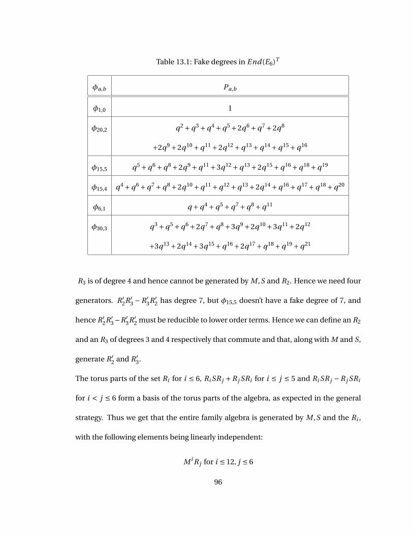
Table 13.1: Fake degrees in End(E6)T
φa,b Pa,b
φ1,0 1
φ20,2 q2 +q3 +q4 +q5 +2q6 +q7 +2q8
+2q9 +2q10 +q11 +2q12 +q13 +q14 +q15 +q16
φ15,5 q5 +q6 +q8 +2q9 +q11 +3q12 +q13 +2q15 +q16 +q18 +q19
φ15,4 q4 +q6 +q7 +q8 +2q10 +q11 +q12 +q13 +2q14 +q16 +q17 +q18 +q20
φ6,1 q +q4 +q5 +q7 +q8 +q11
φ30,3 q3 +q5 +q6 +2q7 +q8 +3q9 +2q10 +3q11 +2q12
+3q13 +2q14 +3q15 +q16 +2q17 +q18 +q19 +q21
R3 is of degree 4 and hence cannot be generated by M ,S and R2. Hence we need four
generators. R ′2R ′
3 −R ′3R ′
2 has degree 7, but φ15,5 doesn’t have a fake degree of 7, and
hence R ′2R ′
3−R ′3R ′
2 must be reducible to lower order terms. Hence we can define an R2
and an R3 of degrees 3 and 4 respectively that commute and that, along with M and S,
generate R ′2 and R ′
3.
The torus parts of the set Ri for i ≤ 6, Ri SR j +R j SRi for i ≤ j ≤ 5 and Ri SR j −R j SRi
for i < j ≤ 6 form a basis of the torus parts of the algebra, as expected in the general
strategy. Thus we get that the entire family algebra is generated by M ,S and the Ri ,
with the following elements being linearly independent:
M i R j for i ≤ 12, j ≤ 6
96
Ri SR j +R j SRi for i ≤ j ≤ 5
Ri SR j −R j SRi for i < j ≤ 6
As in previous cases, multiplying an element by S on both sides yields S times an ele-
ment of I (E6), so we can define d22, d23 and d223 in I (E6) by
d22S = SR22S
d23S = SR2R3S
d223S = SR22R3S
d22 has degree 8, d23 has degree 9 and d223 has degree 12. Moreover, the set
{c1,c2,c3,d22,d23,d223}
is algebraically independent, so d22 must be a C∗-multiple of c4 plus products of lower
degree primitive Casimir operators, d23 must be a C∗-multiple of c5 plus products of
lower degree primitive Casimir operators, and d223 must be a C∗-multiple of c6 plus
products of lower degree primitive Casimir operators. Hence, since we can write R4,
R5 and R6 in terms of c4, c5 and c6, they can be generated by M ,S,R2 and R3. Hence
the entire family algebra can be generated over I (E6) by M ,S,R2 and R3, as stated in
the theorem.
97
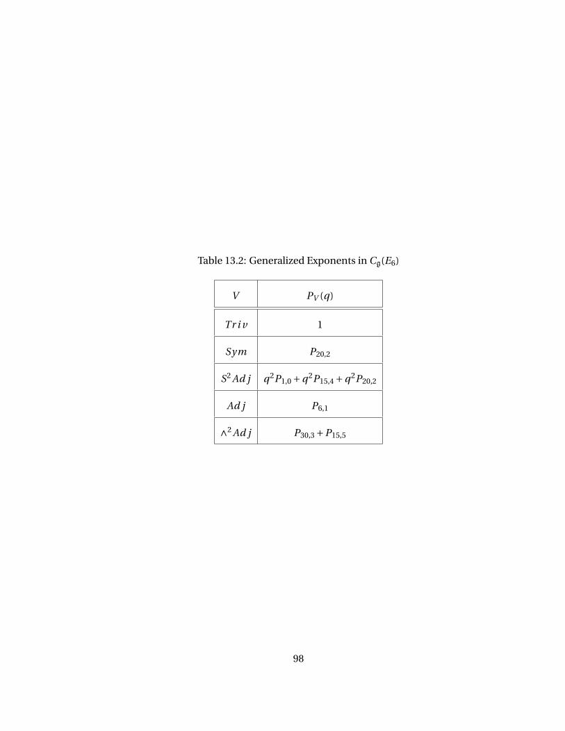
Table 13.2: Generalized Exponents in Cg(E6)
V PV (q)
Tr i v 1
Sym P20,2
S2 Ad j q2P1,0 +q2P15,4 +q2P20,2
Ad j P6,1
∧2 Ad j P30,3 +P15,5
98
Chapter 14
E7
The reference representation of E7 is 56-dimensional, bearing an antisymmetric bilin-
ear form and a symmetric quartic form. We can view it as the Grassman component of
a supervector space whose even part is Euclidean R4, with the metric on R4 becoming
the bilinear form and the determinant on R4 becoming the quartic form.
Alternatively, we can write E7 as a module over A7. We take V to be the standard 8-
dimensional representation of A7, and we take an identification of ∧8V with C, along
with the induced identification of ∧8V ∨ with C. This gives us identifications of ∧kV
with ∧8−kV ∨.
E7 decomposes as E7 = A7 ⊕∧4V , with V being the standard 8-dimensional represen-
tation of A7. For X ∈ A7 and v ∈ ∧4V , we define [X , v] = X .v , and for u, v ∈ ∧4V , we
define [u, v] by ⟨X , [u, v]⟩A7 =−(X .u)∧ v
We can view the 56-dimensional representation as ∧2V ⊕∧2V ∨. The action of A7
99
is the usual action on ∧2V and ∧2V ∨, while the action of u ∈ ∧4V on t ∈ ∧2V is
u.t = u ∧ t ∈∧6V ∼=∧2V ∨ and the action of u on ∧2V ∨ is u.t = u ∧ t ∈∧6V ∨ ∼=∧2V .
Let a,b,c,d ∈∧2V and a∨,b∨c∨,d∨ ∈∧2V ∨. Then we have that the bilinear form looks
like
(a,b) = (a∨,b∨) = 0, (a,b∨) =−(b∨, a) = b∨(a)
and the quadratic form looks like
(a,b,c,d) = a ∧b ∧ c ∧d ∈∧8V ∼=C
(a,b,c,d∨) = 0
(a,b,c∨,d∨) = 1
2c∨(a)d∨(b)+ 1
2d∨(a)c∨(b)− (c∨∧d∨)(a ∧b)
(a,b∨,c∨,d∨) = 0
(a∨,b∨,c∨,d∨) = a∨∧b∨∧ c∨∧d∨ ∈∧8V ∨ ∼=C
with permutations of the arguments treated via the full symmetry of the quadratic
form.
The existence of the bilinear form forces all odd-degree Casimir elements to vanish,
and we are left with the degrees of the primitive Casimir elements being 2,6,8,10,12,14
and 18, with corresponding exponents 1,5,7,9,11,13, and 17.
The torus part of the family algebra decomposes as φ1,0 ⊕φ27,2 ⊕φ21,6, and the vector
part as φ1,0 ⊕φ27,2 ⊕φ35,4 ⊕φ7,1 ⊕φ56,3. See Table 14.1 for the fake degrees of these
representations.
R3 is of degree 6 and hence cannot be generated by M ,S and R2. Hence we need four
100
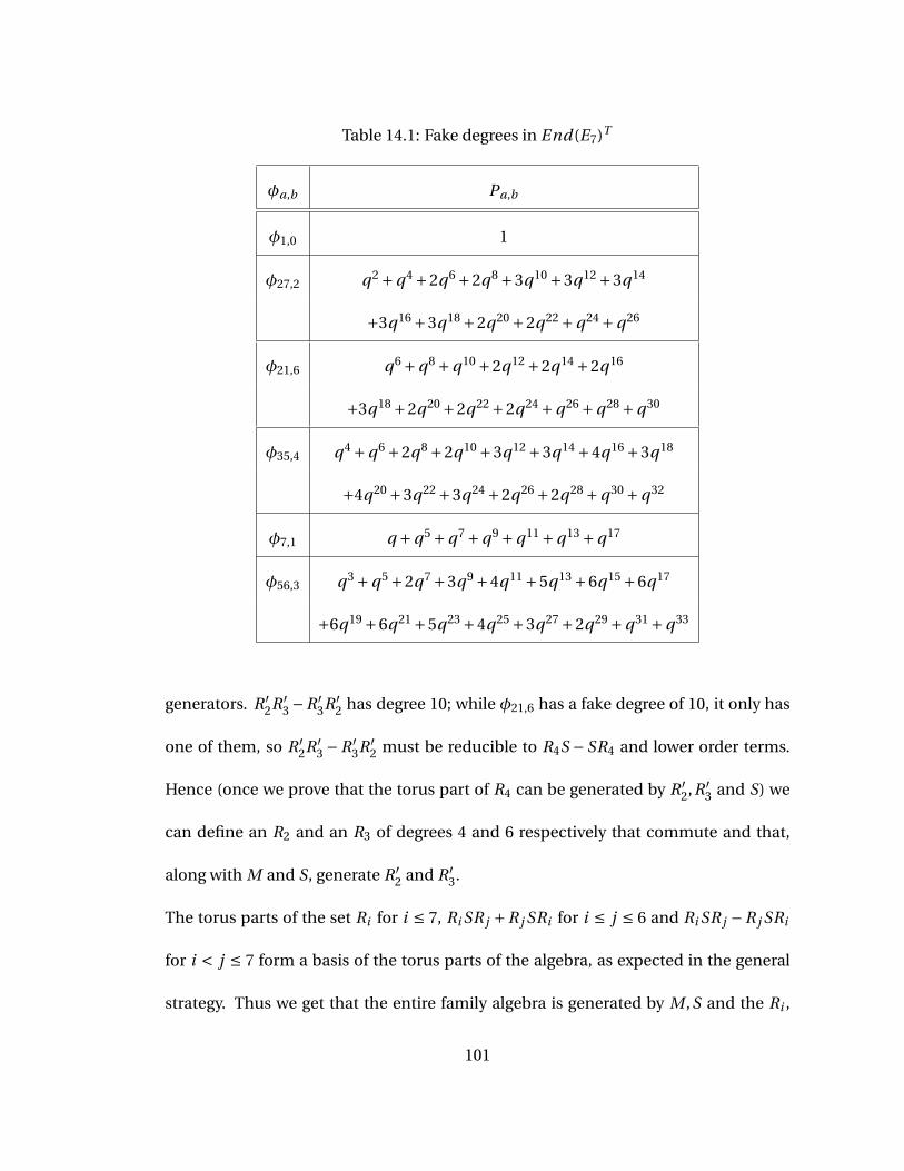
Table 14.1: Fake degrees in End(E7)T
φa,b Pa,b
φ1,0 1
φ27,2 q2 +q4 +2q6 +2q8 +3q10 +3q12 +3q14
+3q16 +3q18 +2q20 +2q22 +q24 +q26
φ21,6 q6 +q8 +q10 +2q12 +2q14 +2q16
+3q18 +2q20 +2q22 +2q24 +q26 +q28 +q30
φ35,4 q4 +q6 +2q8 +2q10 +3q12 +3q14 +4q16 +3q18
+4q20 +3q22 +3q24 +2q26 +2q28 +q30 +q32
φ7,1 q +q5 +q7 +q9 +q11 +q13 +q17
φ56,3 q3 +q5 +2q7 +3q9 +4q11 +5q13 +6q15 +6q17
+6q19 +6q21 +5q23 +4q25 +3q27 +2q29 +q31 +q33
generators. R ′2R ′
3 −R ′3R ′
2 has degree 10; while φ21,6 has a fake degree of 10, it only has
one of them, so R ′2R ′
3 −R ′3R ′
2 must be reducible to R4S − SR4 and lower order terms.
Hence (once we prove that the torus part of R4 can be generated by R ′2,R ′
3 and S) we
can define an R2 and an R3 of degrees 4 and 6 respectively that commute and that,
along with M and S, generate R ′2 and R ′
3.
The torus parts of the set Ri for i ≤ 7, Ri SR j +R j SRi for i ≤ j ≤ 6 and Ri SR j −R j SRi
for i < j ≤ 7 form a basis of the torus parts of the algebra, as expected in the general
strategy. Thus we get that the entire family algebra is generated by M ,S and the Ri ,
101
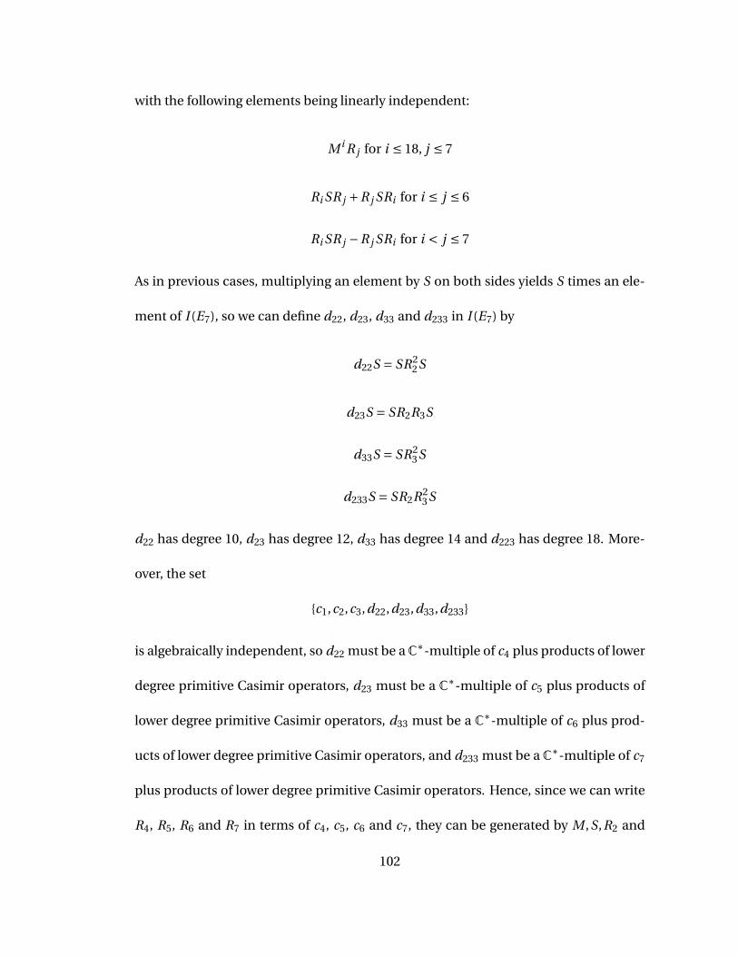
with the following elements being linearly independent:
M i R j for i ≤ 18, j ≤ 7
Ri SR j +R j SRi for i ≤ j ≤ 6
Ri SR j −R j SRi for i < j ≤ 7
As in previous cases, multiplying an element by S on both sides yields S times an ele-
ment of I (E7), so we can define d22, d23, d33 and d233 in I (E7) by
d22S = SR22S
d23S = SR2R3S
d33S = SR23S
d233S = SR2R23S
d22 has degree 10, d23 has degree 12, d33 has degree 14 and d223 has degree 18. More-
over, the set
{c1,c2,c3,d22,d23,d33,d233}
is algebraically independent, so d22 must be a C∗-multiple of c4 plus products of lower
degree primitive Casimir operators, d23 must be a C∗-multiple of c5 plus products of
lower degree primitive Casimir operators, d33 must be a C∗-multiple of c6 plus prod-
ucts of lower degree primitive Casimir operators, and d233 must be a C∗-multiple of c7
plus products of lower degree primitive Casimir operators. Hence, since we can write
R4, R5, R6 and R7 in terms of c4, c5, c6 and c7, they can be generated by M ,S,R2 and
102
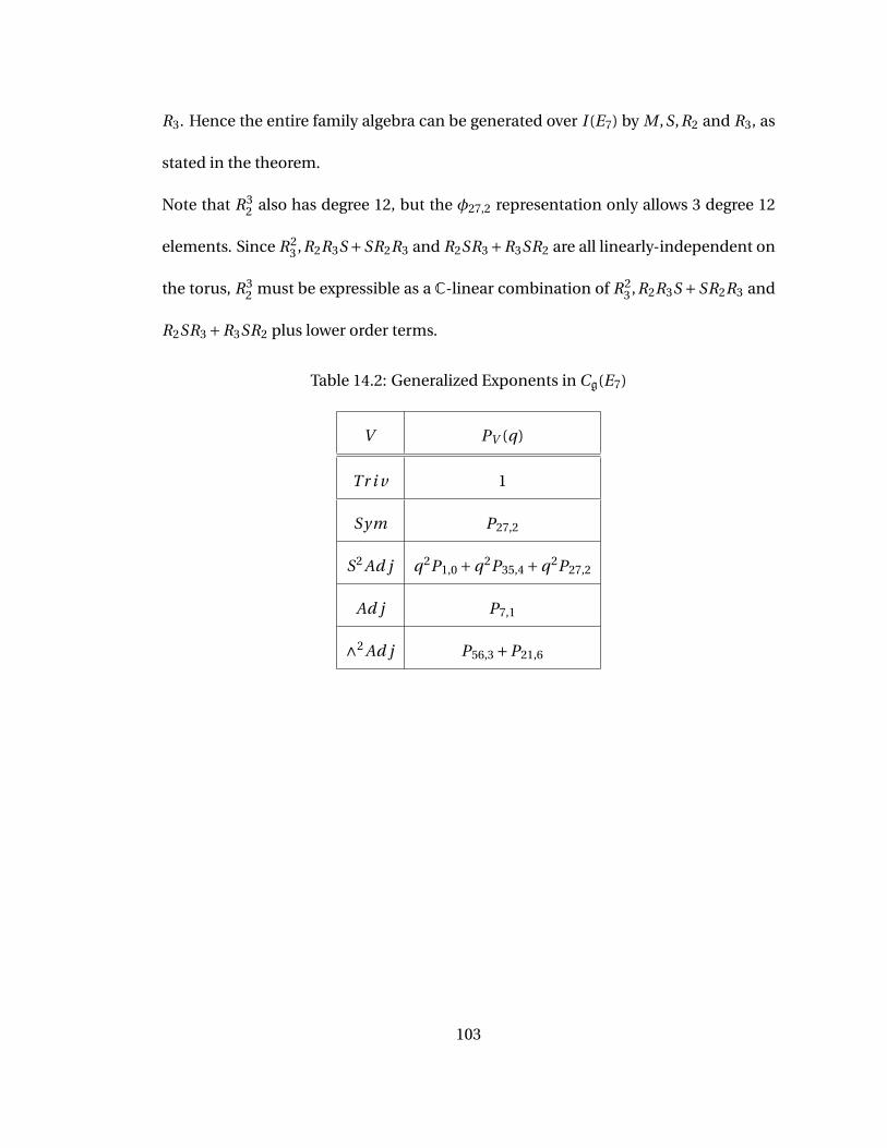
R3. Hence the entire family algebra can be generated over I (E7) by M ,S,R2 and R3, as
stated in the theorem.
Note that R32 also has degree 12, but the φ27,2 representation only allows 3 degree 12
elements. Since R23 ,R2R3S +SR2R3 and R2SR3+R3SR2 are all linearly-independent on
the torus, R32 must be expressible as a C-linear combination of R2
3 ,R2R3S +SR2R3 and
R2SR3 +R3SR2 plus lower order terms.
Table 14.2: Generalized Exponents in Cg(E7)
V PV (q)
Tr i v 1
Sym P27,2
S2 Ad j q2P1,0 +q2P35,4 +q2P27,2
Ad j P7,1
∧2 Ad j P56,3 +P21,6
103
Chapter 15
E8
The reference representation of E8 is the adjoint representation, bearing a symmet-
ric bilinear form (the Killing form) and an antisymmetric trilinear form (the structure
constants). Because the reference representation is the adjoint representation, there
is no nice description of the invariant forms other than as themselves.
Alternatively, we can write E8 as a module over D8. E8 decomposes as E8 = D8 ⊕ S,
where S is one of the two spinor representations of D8; it doesn’t matter which one.
The Lie bracket is extended by [X , s] = X .s for X ∈ D8 and s ∈ S, and for s, t ∈ S, [s, t ] is
defined by ⟨X , [s, t ]⟩D4 = −⟨X .t , s⟩S . The Lie bracket also provides the action of E8 on
itself.
The existence of the bilinear form forces all odd-degree Casimir elements to vanish,
and we are left with the degrees of the primitive Casimir elements being 2,8,12,14,
18,20,24, and 30, with corresponding exponents 1,7,11,13,17, 19,23, and 29.
104
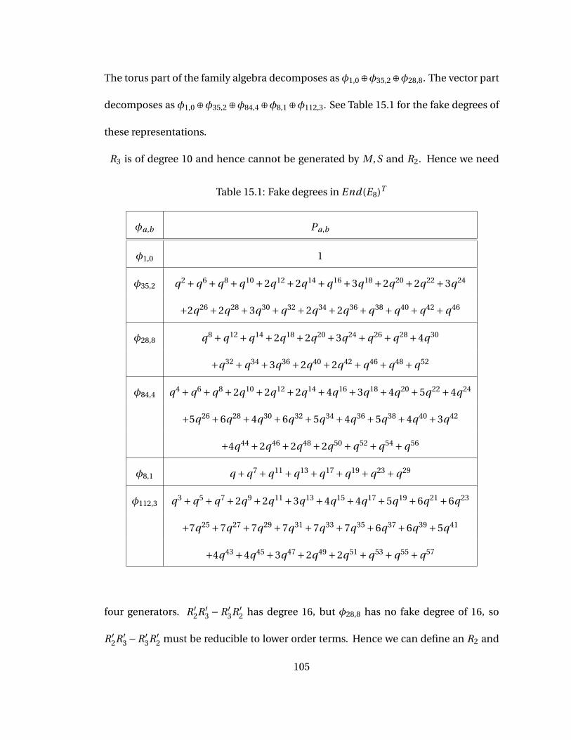
The torus part of the family algebra decomposes as φ1,0⊕φ35,2⊕φ28,8. The vector part
decomposes as φ1,0 ⊕φ35,2 ⊕φ84,4 ⊕φ8,1 ⊕φ112,3. See Table 15.1 for the fake degrees of
these representations.
R3 is of degree 10 and hence cannot be generated by M ,S and R2. Hence we need
Table 15.1: Fake degrees in End(E8)T
φa,b Pa,b
φ1,0 1
φ35,2 q2 +q6 +q8 +q10 +2q12 +2q14 +q16 +3q18 +2q20 +2q22 +3q24
+2q26 +2q28 +3q30 +q32 +2q34 +2q36 +q38 +q40 +q42 +q46
φ28,8 q8 +q12 +q14 +2q18 +2q20 +3q24 +q26 +q28 +4q30
+q32 +q34 +3q36 +2q40 +2q42 +q46 +q48 +q52
φ84,4 q4 +q6 +q8 +2q10 +2q12 +2q14 +4q16 +3q18 +4q20 +5q22 +4q24
+5q26 +6q28 +4q30 +6q32 +5q34 +4q36 +5q38 +4q40 +3q42
+4q44 +2q46 +2q48 +2q50 +q52 +q54 +q56
φ8,1 q +q7 +q11 +q13 +q17 +q19 +q23 +q29
φ112,3 q3 +q5 +q7 +2q9 +2q11 +3q13 +4q15 +4q17 +5q19 +6q21 +6q23
+7q25 +7q27 +7q29 +7q31 +7q33 +7q35 +6q37 +6q39 +5q41
+4q43 +4q45 +3q47 +2q49 +2q51 +q53 +q55 +q57
four generators. R ′2R ′
3 − R ′3R ′
2 has degree 16, but φ28,8 has no fake degree of 16, so
R ′2R ′
3 −R ′3R ′
2 must be reducible to lower order terms. Hence we can define an R2 and
105

an R3 of degrees 6 and 10 respectively that commute and that, along with M and S,
generate R ′2 and R ′
3.
The torus parts of the set Ri for i ≤ 8, Ri SR j +R j SRi for i ≤ j ≤ 7 and Ri SR j −R j SRi
for i < j ≤ 8 form a basis of the torus parts of the algebra, as expected in the general
strategy. Thus we get that the entire family algebra is generated by M ,S and the Ri ,
with the following elements being linearly independent:
M i R j for i ≤ 18, j ≤ 7
Ri SR j +R j SRi for i ≤ j ≤ 6
Ri SR j −R j SRi for i < j ≤ 7
As in previous cases, multiplying an element by S on both sides yields S times an ele-
ment of I (E8), so we can define d22, d23, d222, d223 and d2223 in I (E8) by
d22S = SR22S
d23S = SR2R3S
d222S = SR32S
d223S = SR22R3S
d2223S = SR32R3S
d22 has degree 14, d23 has degree 18, d222 has degree 20, d223 has degree 24, and d2223
has degree 30. Moreover, the set c1,c2,c3,d22,d23,d222, d223 and d2223 is algebraically
106
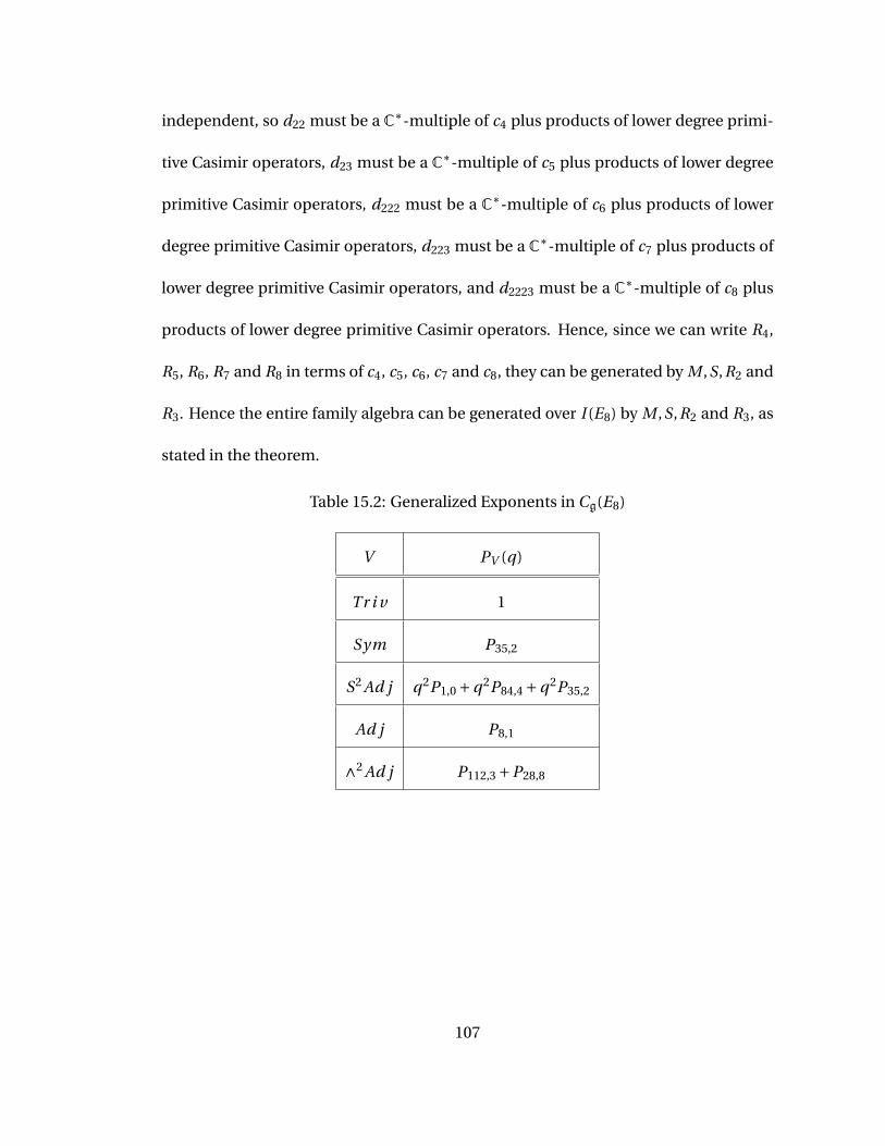
independent, so d22 must be a C∗-multiple of c4 plus products of lower degree primi-
tive Casimir operators, d23 must be a C∗-multiple of c5 plus products of lower degree
primitive Casimir operators, d222 must be a C∗-multiple of c6 plus products of lower
degree primitive Casimir operators, d223 must be a C∗-multiple of c7 plus products of
lower degree primitive Casimir operators, and d2223 must be a C∗-multiple of c8 plus
products of lower degree primitive Casimir operators. Hence, since we can write R4,
R5, R6, R7 and R8 in terms of c4, c5, c6, c7 and c8, they can be generated by M ,S,R2 and
R3. Hence the entire family algebra can be generated over I (E8) by M ,S,R2 and R3, as
stated in the theorem.
Table 15.2: Generalized Exponents in Cg(E8)
V PV (q)
Tr i v 1
Sym P35,2
S2 Ad j q2P1,0 +q2P84,4 +q2P35,2
Ad j P8,1
∧2 Ad j P112,3 +P28,8
107
Bibliography
Be79 Benson, C. T., The generic degrees of the irreducible characters of E8,
Comm. Algebra 7 (1979), 1199-1209
Br95 Broer, B., The sum of generalized exponents and Chevalley’s restric-
tion theorem for modules of covariants, Indag. Math. N.S.6, (1995),
385-396
Ca85 Carter, R. W., Finite Groups of Lie Type: Conjugacy Classes and Com-
plex Characters, John Wiley and Sons, New York, 1985
Cv08 Cvitanovic, P., Group Theory: Birdtracks, Lie’s, and Exceptional
Groups, Princeton University Press, Princeton, NJ, 2008
DLT94 J. Desarmenien, B. Leclerc, J.-Y. Thibon, Hall-Littlewood Functions
and Kostka-Foulkes Polynomials in Representation Theory, Sim.
Lothar. Combin. no 32 (1994), Art. B32c
He80 Hesselink, W. H., Characters of the Nullcone, Math. Ann. 252 (1980),
179-182
108
Ki00 Kirillov, A. A., Family Algebras, Electronic Research Announcements
of the American Mathematical Society, Vol. 6, Mar 1 (2000), 7-20
Ko63 Kostant, B., Lie Group Representations on Polynomial Rings, Ameri-
can Journal of Mathematics, 85 (1963), 327-404
Kn96 Knapp, A., Lie Groups: Beyond an Introduction, Birkhäuser, Boston,
MA, 1996
Lu77 Lusztig, G.Irreducible representations of finite classical groups, In-
vent. Math. 43 (1977) 125–175
Lu79 Lusztig, G., Unipotent representations of a finite Chevalley group of
type E8, Quart. J. Math. Oxford 30 (1979), 315-338
Lu80 Lusztig, G., On the unipotent characters of the exceptional groups
over finite fields, Invent. Math. 60 (1980), 173-192
Mo12 Mostert, P., The q-analogue of the Kostant partition Function and
multiplicities of the zero weight spaces for rank 2 simple Lie algebras,
(2012) unpublished
PW27 Peter, F., Weyl, H., Die Vollständigkeit der primitiven Darstellungen
einer geschlossenen kontinuierlichen Gruppe, Math. Ann. 97 (1927),
737–75
109
RSV99 T. van Ritbergen, A. N. Schellekens, J.A.M. Vermaseren, Group The-
ory Factors for Feynman Diagrams, Int. J. Mod. Phys. A14 (1999), 41-
96
Ro97 Rosenfeld, Boris A., Geometry of Lie Groups, Mathematics and its
Applications 393, Dordrecht: Kluwer Academic Publishers Group,
xviii-393
Ro01 Rojkovskaia, N., Quantum Family Algebras, thesis, 2001
So64 Solomon, L., Invariants of Euclidean Reflection Groups, Trans. Amer.
Math. Soc., 113, (1964), 274-286
Su77 Surowski, D. B., Representatives of a subalgebra of the generic algebra
corresponding to the Weyl group of type F4, Comm. Algebra 5, (1977),
873-888
Su78 Surowski, D. B., Degrees of irreducible characters of B N -pairs of
types E6 and E7, Trans. Amer. Math. Soc., 243 (1978), 235-249
110
![arXiv:1610.09010v3 [math.RT] 26 May 2017Hecke algebras, the Brauer and BMW algebras, walled Brauer algebras, Jones–Temperley–Lieb algebras, as well as centralizer algebras for](https://img.pdfslide.us/doc/110x75/5e54aa9ed50abe21bd3f9542/arxiv161009010v3-mathrt-26-may-2017-hecke-algebras-the-brauer-and-bmw-algebras.jpg)