This paper was posted at http://climatesci.org on May 5, 2009.

Falling Ocean Heat Falsifies Global Warming Hypothesis By William DiPuccio

The Global Warming Hypothesis

Albert Einstein once said, “No amount of experimentation can ever prove me right; a single experiment can prove me wrong.” Einstein’s words express a foundational principle of science intoned by the logician, Karl Popper: Falsifiability. In order to verify a hypothesis there must be a test by which it can be proved false. A thousand observations may appear to verify a hypothesis, but one critical failure could result in its demise. The history of science is littered with such examples.

A hypothesis that cannot be falsified by empirical observations, is not science. The current hypothesis on anthropogenic global warming (AGW), presented by the U.N.’s Intergovernmental Panel on Climate Change (IPCC), is no exception to this principle. Indeed, it is the job of scientists to expose the weaknesses of this hypothesis as it undergoes peer review. This paper will examine one key criterion for falsification: ocean heat.

Ocean heat plays a crucial role in the AGW hypothesis, which maintains that climate change is dominated by human-added, well-mixed green house gasses (GHG). IR radiation that is absorbed and re-emitted by these gases, particularly CO2, is said to be amplified by positive feedback from clouds and water vapor. This process results in a gradual accumulation of heat throughout the climate system, which includes the atmosphere, cryosphere, biosphere, lithosphere, and, most importantly, the hydrosphere. The increase in retained heat is projected to result in rising atmospheric temperatures of 2-6ºC by the year 2100.

In 2005 James Hansen, Josh Willis, and Gavin Schmidt of NASA coauthored a significant article (in collaboration with twelve other scientists), on the “Earth’s Energy Imbalance: Confirmation and Implications” (Science, 3 June 2005, 1431-35). This paper affirmed the critical role of ocean heat as a robust metric for AGW. “Confirmation of the planetary energy imbalance,” they maintained, “can be obtained by measuring the heat content of the ocean, which must be the principal reservoir for excess energy” (1432).

Monotonic Heating. Since the level of CO2 and other well-mixed GHG is on the rise, the overall accumulation of heat in the climate system, measured by ocean heat, should be fairly steady and uninterrupted (monotonic) according to IPCC models, provided there are no major volcanic eruptions. According to the hypothesis, major feedbacks in the climate system are positive (i.e., amplifying), so there is no mechanism in this hypothesis that would cause a suspension or reversal of overall heat accumulation. Indeed, any suspension or reversal would suggest that the heating caused by GHG can be overwhelmed by other human or natural processes in the climate system.

A reversal of sufficient magnitude could conceivably reset the counter back to “zero” (i.e., the initial point from which a current set of measurements began). If this were to take place, the process of heat accumulation would have to start again. In either case, a suspension or reversal of heat accumulation (excepting major volcanic eruptions) would mean that we are dealing with a form of cyclical rather than monotonic heating.

Most scientists who oppose the conclusions of the IPCC have been outspoken in their advocacy of cyclical heating and cooling caused primarily by natural processes, and modified by long-term human climate forcings such as land use change and aerosols. These natural forcings include ocean cycles (PDO, AMO), solar cycles (sunspots, total irradiance), and more speculative causes such as orbital oscillations, and cosmic rays.

Temperature is not Heat!

Despite a consensus among scientists on the use of ocean heat as a robust metric for AGW, near-surface air temperature (referred to as “surface temperature”) is generally employed to gauge global warming. The media and popular culture have certainly equated the two. But this equation is not simply the product of a naïve misunderstanding. NASA’s Goddard Institute for Space Studies (GISS), directed by James Hansen, and the British Hadley Centre for Climate Change, have consistently promoted the use of surface temperature as a metric for global warming. The highly publicized, monthly global surface temperature has become an icon of the AGW projections made by the IPCC.

However, use of surface air temperature as a metric has weak scientific support, except, perhaps, on a multi-decadal or century time-scale. Surface temperature may not register the accumulation of heat in the climate system from year to year. Heat sinks with high specific heat (like water and ice) can absorb (and radiate) vast amounts of heat. Consequently the oceans and the cryosphere can significantly offset atmospheric temperature by heat transfer creating long time lags in surface temperature response time. Moreover, heat is continually being transported in the atmosphere between the poles and the equator. This reshuffling can create fluctuations in average global temperature caused, in part, by changes in cloud cover and water vapor, both of which can alter the earth’s radiative balance.

Hype generated by scientists and institutions over short-term changes in global temperature (up or down) has diverted us from the real issue: heat accumulation. Heat is not the same as temperature. Two liters of boiling water contain twice as much heat as one liter of boiling water even though the water in both vessels is the same temperature. The larger container has more thermal mass which means it takes longer to heat and cool.

Temperature measures the average kinetic energy of molecular motion at a specific point. But it does not measure the total kinetic energy of all the molecules in a substance. In the example above, there is twice as much heat in 2 liters of boiling water because there is twice as much kinetic energy. On average, the molecules in both vessels are moving at the same speed, but the larger container has twice as many molecules.

Temperature may vary from point to point in a moving fluid such as the atmosphere or ocean, but its heat remains constant so long as energy is not added or removed from the system. Consequently, heat-not temperature-is the only sound metric for monitoring the total energy of the climate system. Since heat is a function of both mass and energy, it is normally measured in Joules per kilogram (or calories per gram):

Q = mc∆T

Where Q is heat (Joules)

m is mass (kg)

c is the specific heat constant of the substance (J/kg/°C)

∆T is the change in temperature (°C)

The Thermal Mass of the Oceans

Water is a more appropriate metric for heat accumulation than air because of its ability to store heat. For this reason, it is also a more robust metric for assessing global warming and cooling. Seawater has a much higher mass than air (1030 kg/m3 vs. 1.20 kg/m3at 20ºC), and a higher specific heat (4.18 kJ/kg/°C vs. 1.01 kJ/kg/°C for air at 23°C and 41% humidity). One kilogram of water can retain 4.18x the heat of an equivalent mass of air. This amounts to a thermal mass which is nearly 3558x that of air per unit volume.

For any given area on the ocean’s surface, the upper 2.6m of water has the same heat capacity as the entire atmosphere above it! Considering the enormous depth and global surface area of the ocean (70.5%), it is apparent that its heat capacity is greater than the atmosphere by many orders of magnitude. Consequently, as Hansen, et. al. have concluded, the ocean must be regarded as the main reservoir of atmospheric heat and the primary driver of climate fluctuations.

Heat accumulating in the climate system can be determined by profiling ocean temperature, and from precise measurements of sea surface height as they relate to thermal expansion and contraction of ocean water. These measurements are now possible on a global scale with the ARGO buoy array and from satellite measurements of ocean surface heights. ARGO consists of a world-wide network of over 3000 free-drifting platforms that measure temperature and salinity in the upper 2000m of ocean. The robotic floats rise to the surface every 10 days and transmit data to a satellite which also determines their location.

Pielke’s Litmus Test

In 2007 Roger Pielke, Sr. suggested that ocean heat should be used not just to monitor the energy imbalance in the climate system, but as a “litmus test” for falsifying the IPCC’s AGW hypothesis (Pielke, “A Litmus Test…”, climatesci.org, April 4, 2007). Dr. Pielke is a Senior Research Scientist in CIRES (Cooperative Institute for Research in Environmental Sciences), at the University of Colorado in Boulder, and Professor Emeritus of the Department of Atmospheric Science, Colorado State University, Fort Collins. One of the world’s foremost atmospheric scientists, he has published nearly 350 papers in peer-reviewed journals, 50 chapters in books, and co-edited 9 books.

Pielke’s test compares the net anthropogenic radiative forcing projected by GISS computer models (Hansen, Willis, Schmidt et al.) with actual ocean heat as measured by the ARGO array. To calculate the annual projected heat accumulation in the climate system or oceans, radiative forcing (Watts/m2) must be converted to Joules (Watt seconds) and multiplied by the total surface area of the oceans or earth:

[#1] Qannum = (Ri Pyear Aearth) .80

or, [#2] Qannum = (Ri Pyear Aocean) .85

Where Qannum is the annual heat accumulation in Joules

Ri is the mean global anthropogenic radiative imbalance in W/m2

P is the period of time in seconds/year (31,557,600)

Aocean is the total surface area of the oceans in m2 (3.61132 x 1014)

Aearth is the total surface area of the earth in m2 (5.10072 x 1014)

.80 & .85 are reductions for isolating upper ocean heat (see below)

Radiative Imbalance. The IPCC and GISS calculate the global mean net anthropogenic radiative forcing at ~1.6 W/m2(-1.0, +.8), (see, 2007 IPCC Fourth Assessment Summary for Policy Makers, figure SPM.2 and Hanson, Willis, Schmidt et al., page 1434, Table 1). This is the effective total of all anthropogenic forcings on the climate system. Projected heat accumulation is not calculated from this number, but from the mean global anthropogenic radiative imbalance (Ri). According to Hanson, Willis, Schmidt et al., the imbalance represents that fraction of the total net anthropogenic forcing which the climate system has not yet responded to due to thermal lag (caused primarily by the oceans). The assumption is that since the earth has warmed, a certain amount of energy is required to maintain the current global temperature. Continuing absorption will cause global temperatures to rise further until a new balance is reached.

Physically, the climate system responds to the entire 1.6 W/m2 forcing, not just a portion of it. But while energy is being absorbed, it is also being lost by radiation. The radiative imbalance is better described as the difference between the global mean net anthropogenic radiative forcing and its associated radiative loss. The global radiative imbalance of .75 W/m2 (shown below) would mean that the earth system is radiating .85 W/m2 in response to 1.6 W/m2of total forcing (1.6 - .85 = .75). For a more detailed discussion of radiative equilibrium see, Pielke Sr., R.A., 2003: “Heat storage within the Earth system.” Bulletin of the American Meteorological Society, 84, 331-335.

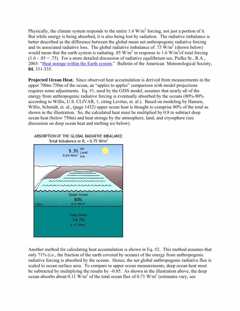
Projected Ocean Heat. Since observed heat accumulation is derived from measurements in the upper 700m-750m of the ocean, an “apples to apples” comparison with model projections requires some adjustments. Eq. #1, used by the GISS model, assumes that nearly all of the energy from anthropogenic radiative forcing is eventually absorbed by the oceans (80%-90% according to Willis, U.S. CLIVAR, 1, citing Levitus, et. al.). Based on modeling by Hansen, Willis, Schmidt, et. al., (page 1432) upper ocean heat is thought to comprise 80% of the total as shown in the illustration. So, the calculated heat must be multiplied by 0.8 to subtract deep ocean heat (below 750m) and heat storage by the atmosphere, land, and cryosphere (see discussion on deep ocean heat and melting ice below).

Another method for calculating heat accumulation is shown in Eq. #2. This method assumes that only 71% (i.e., the fraction of the earth covered by oceans) of the energy from anthropogenic radiative forcing is absorbed by the oceans. Hence, the net global anthropogenic radiative flux is scaled to ocean surface area. To compare to upper ocean measurements, deep ocean heat must be subtracted by multiplying the results by ~0.85. As shown in the illustration above, the deep ocean absorbs about 0.11 W/m2 of the total ocean flux of 0.71 W/m2 (estimates vary, see

discussion on deep ocean heat, below). Since this equation is not used by climate models, it is not included in the following tables. But, it is displayed in the graph below as a possible lower limit of projected heat accumulation.

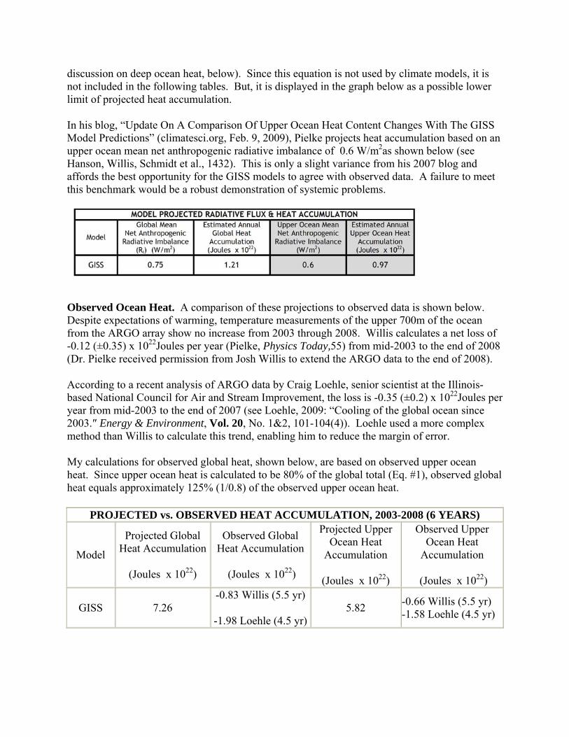
In his blog, “Update On A Comparison Of Upper Ocean Heat Content Changes With The GISS Model Predictions” (climatesci.org, Feb. 9, 2009), Pielke projects heat accumulation based on an upper ocean mean net anthropogenic radiative imbalance of 0.6 W/m2as shown below (see Hanson, Willis, Schmidt et al., 1432). This is only a slight variance from his 2007 blog and affords the best opportunity for the GISS models to agree with observed data. A failure to meet this benchmark would be a robust demonstration of systemic problems.

Observed Ocean Heat. A comparison of these projections to observed data is shown below. Despite expectations of warming, temperature measurements of the upper 700m of the ocean from the ARGO array show no increase from 2003 through 2008. Willis calculates a net loss of -0.12 (±0.35) x 1022Joules per year (Pielke, Physics Today,55) from mid-2003 to the end of 2008 (Dr. Pielke received permission from Josh Willis to extend the ARGO data to the end of 2008).

According to a recent analysis of ARGO data by Craig Loehle, senior scientist at the Illinois-based National Council for Air and Stream Improvement, the loss is -0.35 (±0.2) x 1022Joules per year from mid-2003 to the end of 2007 (see Loehle, 2009: “Cooling of the global ocean since 2003.″ Energy & Environment, Vol. 20, No. 1&2, 101-104(4)). Loehle used a more complex method than Willis to calculate this trend, enabling him to reduce the margin of error.

My calculations for observed global heat, shown below, are based on observed upper ocean heat. Since upper ocean heat is calculated to be 80% of the global total (Eq. #1), observed global heat equals approximately 125% (1/0.8) of the observed upper ocean heat.

PROJECTED vs. OBSERVED HEAT ACCUMULATION, 2003-2008 (6 YEARS)

Model

Projected Global Heat Accumulation

(Joules x 1022)

Observed Global Heat Accumulation

(Joules x 1022)

Projected Upper Ocean Heat

Accumulation

(Joules x 1022)

Observed Upper Ocean Heat

Accumulation

(Joules x 1022)

GISS 7.26 -0.83 Willis (5.5 yr)

-1.98 Loehle (4.5 yr)5.82 -0.66 Willis (5.5 yr)

-1.58 Loehle (4.5 yr)

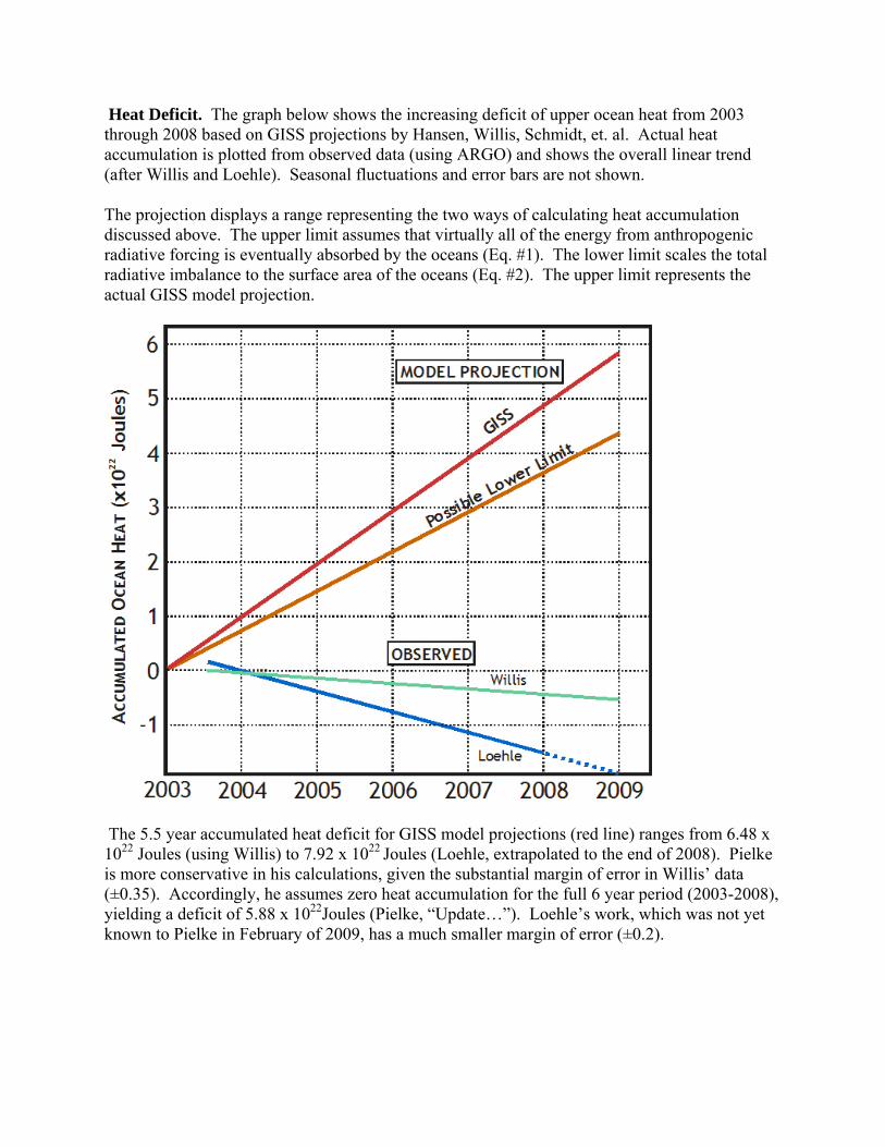
Heat Deficit. The graph below shows the increasing deficit of upper ocean heat from 2003 through 2008 based on GISS projections by Hansen, Willis, Schmidt, et. al. Actual heat accumulation is plotted from observed data (using ARGO) and shows the overall linear trend (after Willis and Loehle). Seasonal fluctuations and error bars are not shown.

The projection displays a range representing the two ways of calculating heat accumulation discussed above. The upper limit assumes that virtually all of the energy from anthropogenic radiative forcing is eventually absorbed by the oceans (Eq. #1). The lower limit scales the total radiative imbalance to the surface area of the oceans (Eq. #2). The upper limit represents the actual GISS model projection.

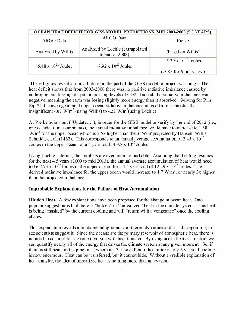
The 5.5 year accumulated heat deficit for GISS model projections (red line) ranges from 6.48 x 1022 Joules (using Willis) to 7.92 x 1022 Joules (Loehle, extrapolated to the end of 2008). Pielke is more conservative in his calculations, given the substantial margin of error in Willis’ data (±0.35). Accordingly, he assumes zero heat accumulation for the full 6 year period (2003-2008), yielding a deficit of 5.88 x 1022Joules (Pielke, “Update…”). Loehle’s work, which was not yet known to Pielke in February of 2009, has a much smaller margin of error (±0.2).

OCEAN HEAT DEFICIT FOR GISS MODEL PREDICTIONS, MID 2003-2008 (5.5 YEARS)

ARGO Data

Analyzed by Willis

ARGO Data

Analyzed by Loehle (extrapolated to end of 2008)

Pielke

(based on Willis)

-6.48 x 1022 Joules -7.92 x 1022 Joules -5.39 x 1022 Joules

(-5.88 for 6 full years )

These figures reveal a robust failure on the part of the GISS model to project warming. The heat deficit shows that from 2003-2008 there was no positive radiative imbalance caused by anthropogenic forcing, despite increasing levels of CO2. Indeed, the radiative imbalance was negative, meaning the earth was losing slightly more energy than it absorbed. Solving for Riin Eq. #1, the average annual upper ocean radiative imbalance ranged from a statistically insignificant -.07 W/m2 (using Willis) to -.22 W/m2(using Loehle).

As Pielke points out (”Update…”), in order for the GISS model to verify by the end of 2012 (i.e., one decade of measurements), the annual radiative imbalance would have to increase to 1.50 W/m2 for the upper ocean which is 2.5x higher than the .6 W/m2projected by Hansen, Willis, Schmidt, et. al. (1432). This corresponds to an annual average accumulation of 2.45 x 1022

Joules in the upper ocean, or a 4 year total of 9.8 x 1022 Joules.

Using Loehle’s deficit, the numbers are even more remarkable. Assuming that heating resumes for the next 4.5 years (2009 to mid 2013), the annual average accumulation of heat would need to be 2.73 x 1022 Joules in the upper ocean, for a 4.5 year total of 12.29 x 1022 Joules. The derived radiative imbalance for the upper ocean would increase to 1.7 W/m2, or nearly 3x higher than the projected imbalance.

Improbable Explanations for the Failure of Heat Accumulation

Hidden Heat. A few explanations have been proposed for the change in ocean heat. One popular suggestion is that there is “hidden” or “unrealized” heat in the climate system. This heat is being “masked” by the current cooling and will “return with a vengeance” once the cooling abates.

This explanation reveals a fundamental ignorance of thermodynamics and it is disappointing to see scientists suggest it. Since the oceans are the primary reservoir of atmospheric heat, there is no need to account for lag time involved with heat transfer. By using ocean heat as a metric, we can quantify nearly all of the energy that drives the climate system at any given moment. So, if there is still heat “in the pipeline”, where is it? The deficit of heat after nearly 6 years of cooling is now enormous. Heat can be transferred, but it cannot hide. Without a credible explanation of heat transfer, the idea of unrealized heat is nothing more than an evasion.

Deep Ocean Heat. Is it possible that “lost” heat has been transferred to the deep ocean-below the 700 meter limit of our measurements? This appears unlikely. According to Hansen, Willis, Schmidt et al., model simulations of ocean heat flow show that 85% of heat storage occurs above 750 m on average (with the range stretching from 78 to 91%) (1432). Moreover, if there is “buried” heat, widespread diffusion and mixing with bottom waters may render it statistically irrelevant in terms of its impact on climate.

The absence of heat accumulation in deep water is corroborated by a recent study of ocean mass and altimetric sea level by Cazenave, et. al. Deep water heat should produce thermal expansion, causing sea level to rise. Instead, steric sea level (which measures thermal expansion plus salinity effects) peaked near the end of 2005, then began to decline nearly steadily. It appears that ocean volume has actually contracted slightly.

Melting Ice. Another possibility is that meltwater from glaciers, sea ice, and ice caps is offsetting heat accumulation. Perhaps the ocean temperature has plateaued as the ice undergoes a phase change from solid to liquid (heat of fusion).

This explanation sounds plausible at first, but it is not supported by observed data or best estimates. In a 2001 paper published in Science, Levitus, et. al. calculates that the absorption of heat due to melting ice amounts to only 6.85% of the total increase in ocean heat during the 41 year period from about 1955 to 1996:

Observed increase in ocean heat (1955-1996) = 1.82 x 1023 J

Observed/estimated heat of fusion (1950’s-1990’s) = 1.247 x 1022 J

This work is quoted by Hansen, Willis, Schmidt, et. al. and further supported by their calculations (1432), which are even more conservative. Given a planetary energy imbalance of approximately +0.75 W/m2, their simulations show that only 5.3% (0.04 W/m2) of the energy is used to warm the atmosphere, the land, and melt ice. The balance of energy is absorbed by the ocean above 750 m (~0.6 W/m2), with a small amount of energy penetrating below 750 m (~0.11 W/m2).

The absorption of heat by melting ice is so small that even if it were to quadruple, the impact on ocean heat would be miniscule.

Cold Biasing. The ARGO array does not provide total geographic coverage. Ocean areas beneath ice are not measured. However, this would have a relatively small impact on total ocean heat since it comprises less than 7% of the ocean. As mentioned above, quality controlled water temperature below 700m is not available, though the floats operate to a depth of 2000m. Above 700m, the analysis performed by Willis includes a quality check of raw data which revealed a cold bias in some instruments. This bias was removed (Willis, CLIVAR, 1).

Loehle warns that the complexities of instrumental drift could conceivably create such artifacts (Loehle, 101), but concludes that his analysis is consistent with satellite and surface data which show no warming for the same period (e.g., see Douglass, D.H., J.R. Christy, 2009: “Limits on

CO2 climate forcing from recent temperature data of Earth.” Energy & Environment, Vol. 20, No. 1&2, 178-189 (13)). So it is unlikely that cold biasing could account for the observed changes in ocean heat.

In brief, we know of no mechanism by which vast amounts of “missing” heat can be hidden, transferred, or absorbed within the earth’s system. The only reasonable conclusion-call it a null hypothesis-is that heat is no longer accumulating in the climate system and there is no longer a radiative imbalance caused by anthropogenic forcing. This not only demonstrates that the IPCC models are failing to accurately predict global warming, but also presents a serious challenge to the integrity of the AGW hypothesis.

Analysis and Conclusion

Though other criteria, such as climate sensitivity (Spencer, Lindzen), can be used to test the AGW hypothesis, ocean heat has one main advantage: Simplicity. While work on climate sensitivity certainly needs to continue, it requires more complex observations and hypotheses making verification more difficult. Ocean heat touches on the very core of the AGW hypothesis: When all is said and done, if the climate system is not accumulating heat, the hypothesis is invalid.

Writing in 2005, Hansen, Willis, Schmidt et al. suggested that GISS model projections had been verified by a solid decade of increasing ocean heat (1993 to 2003). This was regarded as further confirmation the IPCC’s AGW hypothesis. Their expectation was that the earth’s climate system would continue accumulating heat more or less monotonically. Now that heat accumulation has stopped (and perhaps even reversed), the tables have turned. The same criteria used to support their hypothesis, is now being used to falsify it.

It is evident that the AGW hypothesis, as it now stands, is either false or fundamentally inadequate. One may argue that projections for global warming are measured in decades rather than months or years, so not enough time has elapsed to falsify this hypothesis. This would be true if it were not for the enormous deficit of heat we have observed. In other words, no matter how much time has elapsed, if a projection misses its target by such a large magnitude (6x to 8x), we can safely assume that it is either false or seriously flawed.

Assuming the hypothesis is not false, its proponents must now address the failure to skillfully project heat accumulation. Theories pass through stages of development as they are tested against observations. It is possible that the AGW hypothesis is not false, but merely oversimplified. Nevertheless, any refinements must include causal mechanisms which are testable and falsifiable. Arm waiving and ad hoc explanations (such as large margins of error) are not sufficient.

One possibility for the breakdown may relate back to climate sensitivity. It is assumed that most feedbacks are positive, amplifying the slight warming (.3º-1.2ºC) caused by CO2. This may only be partially correct. Perhaps these feedbacks undergo quasi-cyclical changes in tandem with natural fluctuations in climate. The net result might be a more punctuated increase in heat accumulation with possible reversals, rather than a monotonic increase. The outcome would be a

much slower rate of warming than currently projected. This would make it difficult to isolate and quantify anthropogenic forcing against the background noise of natural climate signals.

On the other hand, the current lapse in heat accumulation demonstrates a complete failure of the AGW hypothesis to account for natural climate variability, especially as it relates to ocean cycles (PDO, AMO, etc.). If anthropogenic forcing from GHG can be overwhelmed by natural fluctuations (which themselves are not fully understood), or even by other types of anthropogenic forcing, then it is not unreasonable to conclude that the IPCC models have little or no skill in projecting global and regional climate change on a multi-decadal scale. Dire warnings about “runaway warming” and climate “tipping points” cannot be taken seriously. A complete rejection of the hypothesis, in its current form, would certainly be warranted if the ocean continues to cool (or fails to warm) for the next few years.

Whether the anthropogenic global warning hypothesis is invalid or merely incomplete, the time has come for serious debate and reanalysis. Since Dr. Pielke first published his challenge in 2007, no critical attempts have been made to explain these failed projections. His blogs have been greeted by the chirping of crickets. In the mean time costly political agendas focused on carbon mitigation continue to move forward, oblivious to recent empirical evidence. Open and honest debate has been marginalized by appeals to consensus. But as history has often shown, consensus is the last refuge of poor science.

References

Cazenave, A., et al., 2008: “Sea level budget over 2003-2008: A reevaluation from GRACE space gravimetry, satellite altimetry and Argo,” Glob. Planet. Change, doi:10.1016/j.gloplacha.2008.10.004.

Douglass, D.H., J.R. Christy, 2009: “Limits on CO2 climate forcing from recent temperature data of Earth.” Energy & Environment, Vol. 20, No. 1&2, 178-189 (13).

Hansen, J., L. Nazarenko, R. Ruedy, Mki. Sato, J. Willis, A. Del Genio, D. Koch, A. Lacis, K. Lo, S. Menon, T. Novakov, Ju. Perlwitz, G. Russell, G.A. Schmidt, and N. Tausnev, 2005: “Earth’s energy imbalance: Confirmation and implications.” Science, 308, 1431-1435.

IPCC, 2007: Summary for Policymakers. In: Climate Change 2007: The Physical Science Basis. Contribution of Working Group I to the Fourth Assessment Report of the Intergovernmental Panel on Climate Change[Solomon, S., D. Qin, M. Manning, Z. Chen, M. Marquis, K.B. Averyt, M.Tignor and H.L. Miller (eds.)]. Cambridge University Press, Cambridge, United Kingdom and New York, NY, USA. See www.ipcc.ch/pdf/assessment-report/ar4/wg1/ar4-wg1-spm.pdf

Levitus, S., J.I. Antonov, J. Wang, T.L. Delworth, K.W. Dixon, and A.J. Broccoli, 2001: “Anthropogenic warming of Earth’s climate system.” Science, 292, 267-268.

Loehle, Craig, 2009: “Cooling of the global ocean since 2003.″ Energy & Environment, Vol. 20, No. 1&2, 101-104(4).

Pielke Sr., R.A., 2008: “A broader view of the role of humans in the climate system.” Physics Today, 61, Vol. 11, 54-55.

Pielke Sr., R.A., 2003: “Heat storage within the Earth system.” Bulletin of the American Meteorological Society, 84, 331-335.

Pielke Sr., R.A., “A Litmus Test For Global Warming - A Much Overdue Requirement“, climatesci.org, April 4, 2007.

Pielke Sr., R.A., “Update On A Comparison Of Upper Ocean Heat Content Changes With The GISS Model Predictions“, climatesci.org, Feb. 9, 2009.

Willis, J.K., D. Roemmich, and B. Cornuelle, 2004: “Interannual variability in upper ocean heat content, temperature, and thermosteric expansion on global scales.” J. Geophys. Res., 109, C12036.

Willis, J. K., 2008: “Is it Me, or Did the Oceans Cool?”, U.S. CLIVAR, Sept, 2008, Vol. 6, No. 2.

* William DiPuccio was a weather forecaster for the U.S. Navy, and a Meteorological/Radiosonde Technician for the National Weather Service. More recently, he served as head of the science department for St. Nicholas Orthodox School in Akron, Ohio (closed in 2006). He continues to write science curriculum, publish articles, and conduct science camps.