Falling Behind: Bank Data on the Role of Income and

1

October 2018

Falling Behind: Bank Data on the Role of Income and Savings in Mortgage DefaultBy Diana Farrell, Kanav Bhagat, and Chen Zhao

IntroductionFor many American households, buying a home represents one of their largest lifetime expenditures. And because most homeowners finance

their home purchase with a mortgage, buying a home is also one of their largest sources of debt. In our report Mortgage Modifications

after the Great Recession: New Evidence and Implications for Policy, we measured the impact of mortgage payment and principal reduction

on default and consumption. We found that a 10 percent mortgage payment reduction decreased default rates by 22 percent, whereas for

borrowers who remained underwater, principal reduction had no effect on default or consumption. This finding implies that short term

liquidity was a key factor driving mortgage default.

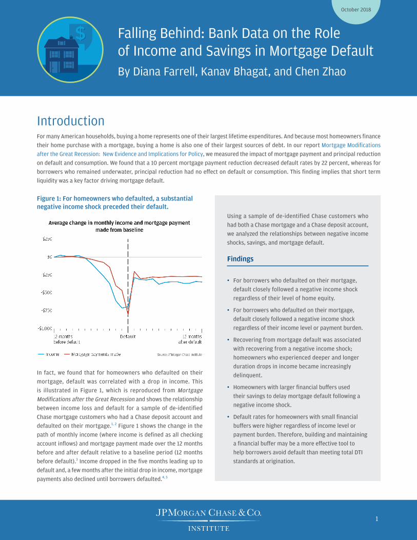
Figure 1: For homeowners who defaulted, a substantial negative income shock preceded their default.

Using a sample of de-identified Chase customers who

had both a Chase mortgage and a Chase deposit account,

we analyzed the relationships between negative income

shocks, savings, and mortgage default.

Findings

• For borrowers who defaulted on their mortgage,

default closely followed a negative income shock

regardless of their level of home equity.

• For borrowers who defaulted on their mortgage,

default closely followed a negative income shock

regardless of their income level or payment burden.

• Recovering from mortgage default was associated

with recovering from a negative income shock;

homeowners who experienced deeper and longer

duration drops in income became increasingly

delinquent.

• Homeowners with larger financial buffers used

their savings to delay mortgage default following a

negative income shock.

• Default rates for homeowners with small financial

buffers were higher regardless of income level or

payment burden. Therefore, building and maintaining

a financial buffer may be a more effective tool to

help borrowers avoid default than meeting total DTI

standards at origination.

In fact, we found that for homeowners who defaulted on their

mortgage, default was correlated with a drop in income. This

is illustrated in Figure 1, which is reproduced from Mortgage

Modifications after the Great Recession and shows the relationship

between income loss and default for a sample of de-identified

Chase mortgage customers who had a Chase deposit account and

defaulted on their mortgage.1, 2 Figure 1 shows the change in the

path of monthly income (where income is defined as all checking

account inflows) and mortgage payment made over the 12 months

before and after default relative to a baseline period (12 months

before default).3 Income dropped in the five months leading up to

default and, a few months after the initial drop in income, mortgage

payments also declined until borrowers defaulted.4, 5

https://www.jpmorganchase.com/corporate/institute/report-mortgage-modifications-after-recession.htm

JPMorgan Chase InstituteFalling Behind: Bank Data on the Role of Income and Savings in Mortgage Default

2

In this follow-up research to our Mortgage Modifications after the Great Recession report, we further examined the relationship between

income shocks and mortgage default. We found that the relationship between negative income shocks and mortgage default illustrated

in Figure 1 held for homeowners across all levels of home equity and regardless of income level or total debt-to-income ratio (DTI) at

origination. Deeper and longer duration negative income shocks were associated with increasing delinquency, whereas to the extent

their income recovered quickly, homeowners promptly resumed making their mortgage payments. Homeowners with savings used their

financial buffer to delay mortgage default following a negative income shock. Finally, we examined the relationships between financial

buffers, income, payment burden, and default rates. Homeowners with larger financial buffers had lower default rates regardless of their

income level or payment burden.

Taken together, these findings suggest that providing borrowers with an incentive to build and maintain a post-purchase financial

buffer may be a more effective approach to default prevention than underwriting standards based on meeting ability-to-repay rules

at origination.


3

Finding One

For borrowers who defaulted on their mortgage, default closely followed a negative income shock regardless of their level of home equity.

In Mortgage Modifications after the Great Recession, we separately examined above water and underwater households and found that

for both groups, default followed shortly after a negative income shock. But was the relationship between income and mortgage default

different for borrowers with substantial negative equity? To answer this question, we divided our sample into more granular loan-to-value

(LTV) bands. Specifically, we divided the above water households into those with an LTV below 80 percent and those with an LTV between

80 and 100 percent. Similarly, we divided the underwater households into those with an LTV between 100 and 130 percent and those with

an LTV above 130 percent in order to isolate borrowers with a large amount of negative equity.

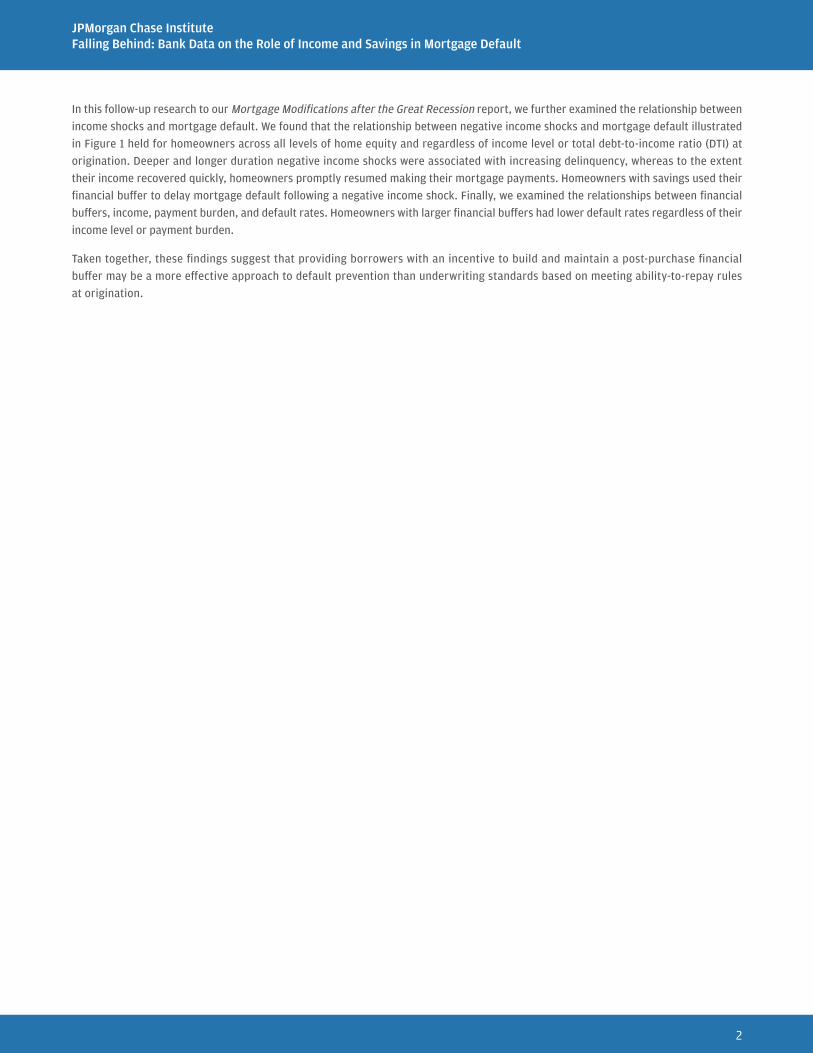
The results for each LTV group are illustrated in the four panels of Figure 2, each of which is analogous to Figure 1, showing the change in the

path of monthly income and mortgage payment made over the 12 months before and after default relative to a baseline month (12 months

before default). Figure 2 only includes households for whom we observe LTV at default.6 In each panel of Figure 2, the pattern is similar to the

pattern in Figure 1: income steadily dropped in the months leading up to default, regardless of the borrower’s home equity.

The similarity in the relationship between income shock and default for various LTVs provides further evidence that underwater borrowers,

including those who were deeply underwater, did not default only because they owed more on their mortgage than their house was worth.

If some borrowers were defaulting simply because they were underwater, our data would show a smaller drop in inflows around default for

borrowers with high amounts of negative equity, such as those with an LTV above 130 percent. Instead, the income drop experienced by

borrowers with an LTV above 130 percent is similar in magnitude to the income drop experienced by lower LTV borrowers. Therefore, our

data are inconsistent with this simple type of strategic default.7

Figure 2: Default followed a negative income shock for borrowers across the LTV distribution, providing suggestive evidence against a simple model of strategic default where deeply underwater borrowers stop making mortgage payments only because they are underwater.


4

Finding Two

For borrowers who defaulted on their mortgage, default closely followed a negative income shock regardless of their income level or payment burden.

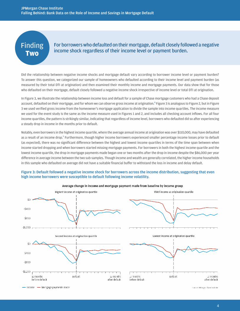
Did the relationship between negative income shocks and mortgage default vary according to borrower income level or payment burden?

To answer this question, we categorized our sample of homeowners who defaulted according to their income level and payment burden (as

measured by their total DTI at origination) and then examined their monthly income and mortgage payments. Our data show that for those

who defaulted on their mortgage, default closely followed a negative income shock irrespective of income level or total DTI at origination.

In Figure 3, we illustrate the relationship between income loss and default for a sample of Chase mortgage customers who had a Chase deposit

account, defaulted on their mortgage, and for whom we can observe gross income at origination.8 Figure 3 is analogous to Figure 2, but in Figure

3 we used verified gross income from the homeowner’s mortgage application to divide the sample into income quartiles. The income measure

we used for the event study is the same as the income measure used in Figures 1 and 2, and includes all checking account inflows. For all four

income quartiles, the pattern is strikingly similar, indicating that regardless of income level, borrowers who defaulted did so after experiencing

a steady drop in income in the months prior to default.

Notably, even borrowers in the highest income quartile, where the average annual income at origination was over $110,000, may have defaulted

as a result of an income drop.9 Furthermore, though higher income borrowers experienced smaller percentage income losses prior to default

(as expected), there was no significant difference between the highest and lowest income quartiles in terms of the time span between when

income started dropping and when borrowers started missing mortgage payments. For borrowers in both the highest income quartile and the

lowest income quartile, the drop in mortgage payments made began one or two months after the drop in income despite the $86,000 per year

difference in average income between the two sub-samples. Though income and wealth are generally correlated, the higher income households

in this sample who defaulted on average did not have a suitable financial buffer to withstand the loss in income and delay default.

Figure 3: Default followed a negative income shock for borrowers across the income distribution, suggesting that even high income borrowers were susceptible to default following income volatility.


5

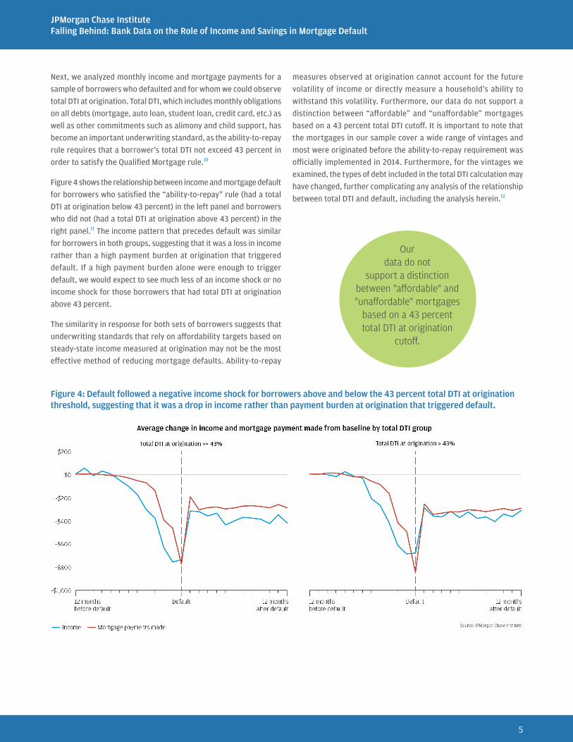
Next, we analyzed monthly income and mortgage payments for a

sample of borrowers who defaulted and for whom we could observe

total DTI at origination. Total DTI, which includes monthly obligations

on all debts (mortgage, auto loan, student loan, credit card, etc.) as

well as other commitments such as alimony and child support, has

become an important underwriting standard, as the ability-to-repay

rule requires that a borrower’s total DTI not exceed 43 percent in

order to satisfy the Qualified Mortgage rule.10

Figure 4 shows the relationship between income and mortgage default

for borrowers who satisfied the “ability-to-repay” rule (had a total

DTI at origination below 43 percent) in the left panel and borrowers

who did not (had a total DTI at origination above 43 percent) in the

right panel.11 The income pattern that precedes default was similar

for borrowers in both groups, suggesting that it was a loss in income

rather than a high payment burden at origination that triggered

default. If a high payment burden alone were enough to trigger

default, we would expect to see much less of an income shock or no

income shock for those borrowers that had total DTI at origination

above 43 percent.

The similarity in response for both sets of borrowers suggests that

underwriting standards that rely on affordability targets based on

steady-state income measured at origination may not be the most

effective method of reducing mortgage defaults. Ability-to-repay

measures observed at origination cannot account for the future

volatility of income or directly measure a household’s ability to

withstand this volatility. Furthermore, our data do not support a

distinction between “affordable” and “unaffordable” mortgages

based on a 43 percent total DTI cutoff. It is important to note that

the mortgages in our sample cover a wide range of vintages and

most were originated before the ability-to-repay requirement was

officially implemented in 2014. Furthermore, for the vintages we

examined, the types of debt included in the total DTI calculation may

have changed, further complicating any analysis of the relationship

between total DTI and default, including the analysis herein.12

Our data do not

support a distinction between "affordable" and "unaffordable" mortgages

based on a 43 percent total DTI at origination

cutoff.

Figure 4: Default followed a negative income shock for borrowers above and below the 43 percent total DTI at origination threshold, suggesting that it was a drop in income rather than payment burden at origination that triggered default.


6

Finding Three

Recovering from mortgage default was associated with recovering from a negative income shock; homeowners who experienced deeper and longer duration drops in income became increasingly delinquent.

In the previous findings, we presented evidence that default closely

followed a negative income shock for borrowers across the income

spectrum. We now turn to the question of what happened in the

months following default. How should we interpret the partial recovery

in income after default that is evident in Figure 1? For borrowers who

defaulted, was there a continued connection between their paths of

income and their state of delinquency in the months that followed

default? To answer these questions, we categorized homeowners

who defaulted according to their status in the month after they

defaulted (less delinquent, similarly delinquent, or more delinquent)

and then observed the path of their incomes.13 We found that the

income of homeowners who became more delinquent exhibited larger

negative shocks and recovered to a lesser extent than the incomes of

homeowners who resumed making mortgage payments.

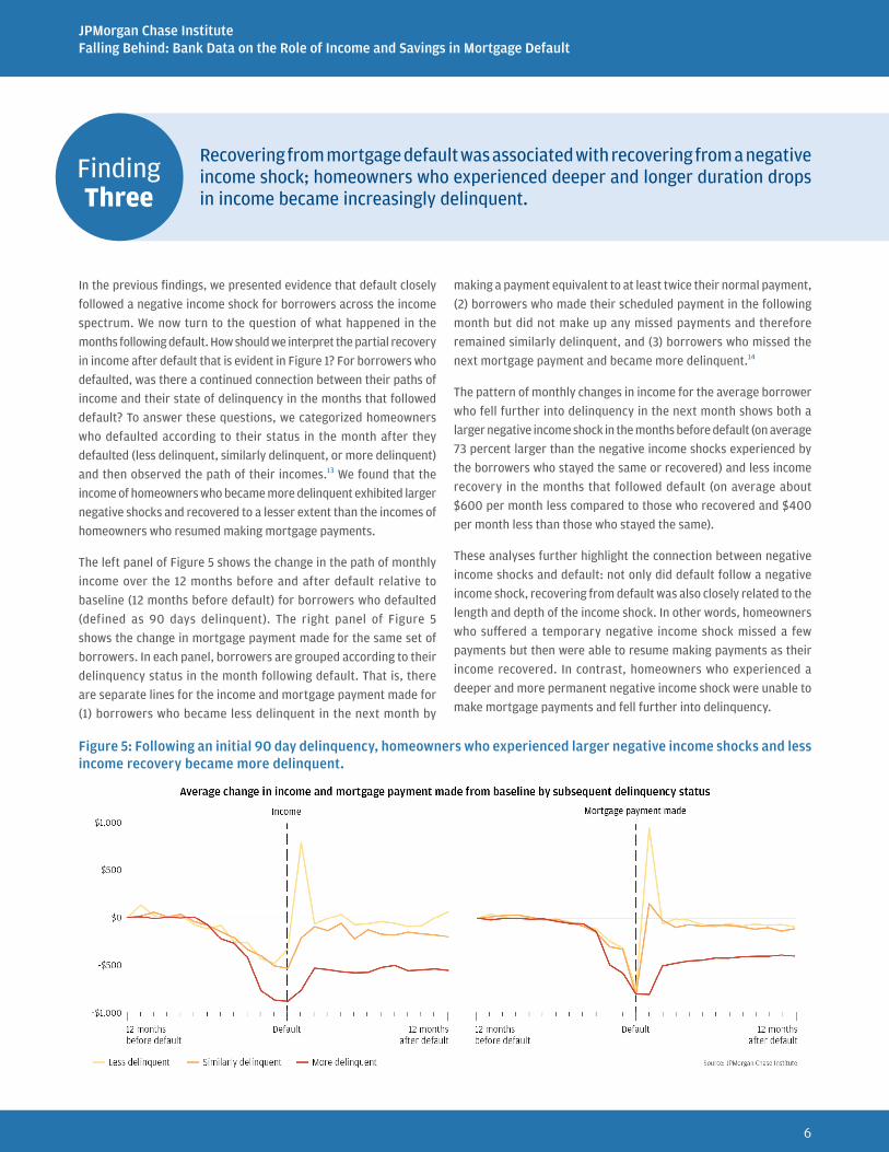
The left panel of Figure 5 shows the change in the path of monthly

income over the 12 months before and after default relative to

baseline (12 months before default) for borrowers who defaulted

(defined as 90 days delinquent). The right panel of Figure 5

shows the change in mortgage payment made for the same set of

borrowers. In each panel, borrowers are grouped according to their

delinquency status in the month following default. That is, there

are separate lines for the income and mortgage payment made for

(1) borrowers who became less delinquent in the next month by

making a payment equivalent to at least twice their normal payment,

(2) borrowers who made their scheduled payment in the following

month but did not make up any missed payments and therefore

remained similarly delinquent, and (3) borrowers who missed the

next mortgage payment and became more delinquent.14

The pattern of monthly changes in income for the average borrower

who fell further into delinquency in the next month shows both a

larger negative income shock in the months before default (on average

73 percent larger than the negative income shocks experienced by

the borrowers who stayed the same or recovered) and less income

recovery in the months that followed default (on average about

$600 per month less compared to those who recovered and $400

per month less than those who stayed the same).

These analyses further highlight the connection between negative

income shocks and default: not only did default follow a negative

income shock, recovering from default was also closely related to the

length and depth of the income shock. In other words, homeowners

who suffered a temporary negative income shock missed a few

payments but then were able to resume making payments as their

income recovered. In contrast, homeowners who experienced a

deeper and more permanent negative income shock were unable to

make mortgage payments and fell further into delinquency.

Figure 5: Following an initial 90 day delinquency, homeowners who experienced larger negative income shocks and less income recovery became more delinquent.


7

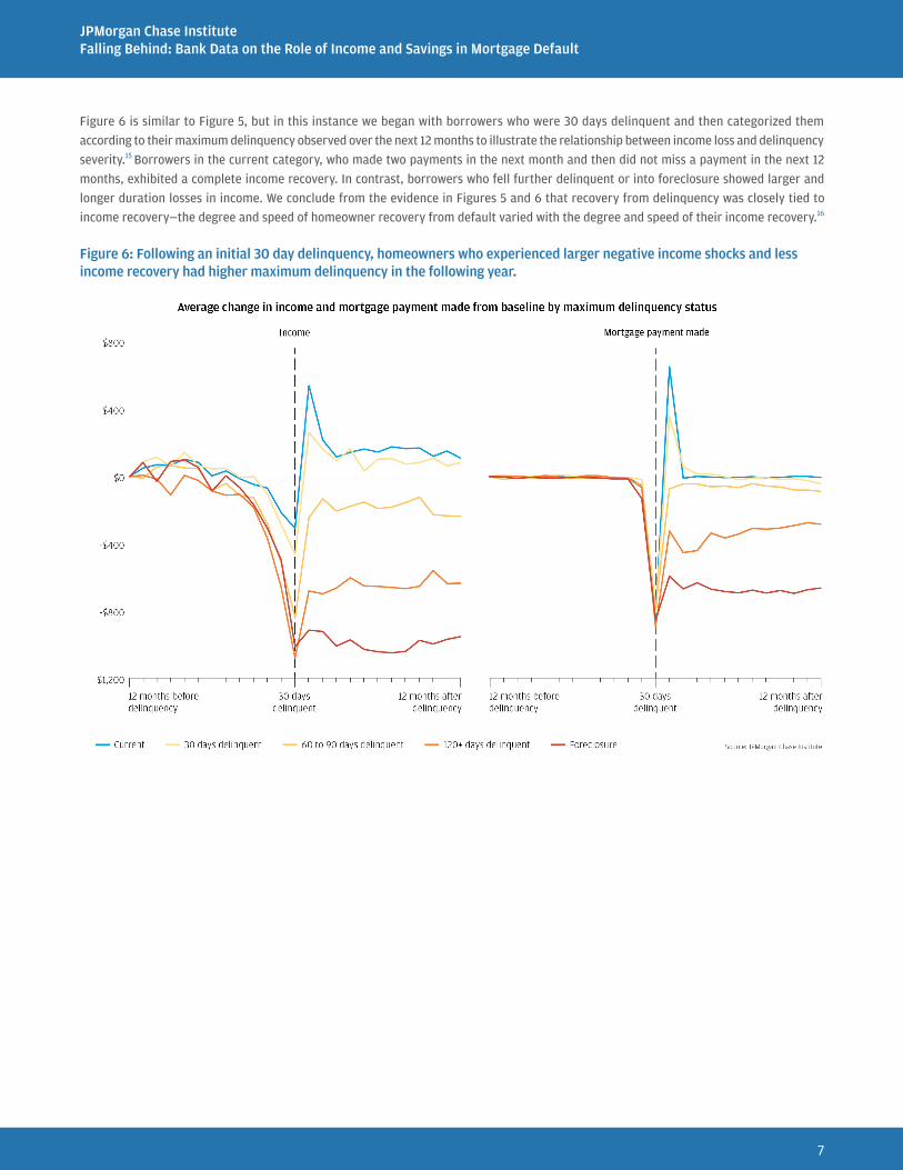
Figure 6 is similar to Figure 5, but in this instance we began with borrowers who were 30 days delinquent and then categorized them

according to their maximum delinquency observed over the next 12 months to illustrate the relationship between income loss and delinquency

severity.15 Borrowers in the current category, who made two payments in the next month and then did not miss a payment in the next 12

months, exhibited a complete income recovery. In contrast, borrowers who fell further delinquent or into foreclosure showed larger and

longer duration losses in income. We conclude from the evidence in Figures 5 and 6 that recovery from delinquency was closely tied to

income recovery—the degree and speed of homeowner recovery from default varied with the degree and speed of their income recovery.16

Figure 6: Following an initial 30 day delinquency, homeowners who experienced larger negative income shocks and less income recovery had higher maximum delinquency in the following year.


8

Finding Four

Homeowners with larger financial buffers used their savings to delay mortgage default following a negative income shock.

In the previous findings we presented evidence that mortgage default closely followed an income shock and that the extent to which

borrowers recovered from default was closely tied to the extent to which their income recovered. What might help borrowers delay

default? Intuition suggests that having savings might help delay default after an income shock, so we turn to an examination of the role

of financial buffers.

We begin with a sample of de-identified Chase customers with a deposit account who defaulted on their mortgage and then split this

sample by above-median and below-median deposit account balance.17 We measure deposit account balances as the sum of checking

and savings account balances and will use the term “financial buffer” to refer to this measure.

Figure 7 shows the change in the path of monthly income, mortgage payment made, and deposit account balance over the 12 months

before and after default relative to baseline (12 months before default) for homeowners in the below-median (less than $794) deposit

account balance group in the left panel and above-median (greater than $794) deposit account balance group in the right panel. The

baseline deposit account balance is the average over the 6-month period 18 to 13 months prior to default.

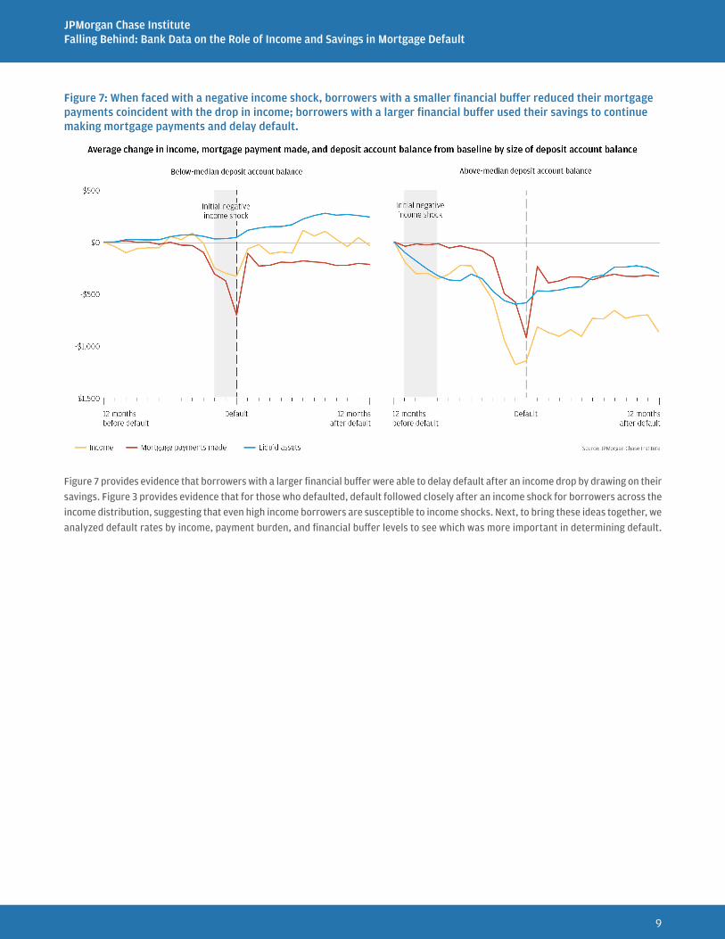
The average borrower in the sub-sample with a below-median deposit account balance (left panel of Figure 7) had a monthly mortgage

payment of about $780 and an average daily balance of about $400 in their deposit accounts at baseline, which means they were holding

less than one mortgage payment equivalent in reserve.18 For this sub-sample, the drop in mortgage payment made coincided with

their drop in income. On average, these borrowers had little in reserves, and therefore a negative income shock led directly to reduced

mortgage payments in the very same month. Three months after income first dropped, these borrowers entered default (defined as 90

day delinquency).

In contrast, the average borrower in the above-median deposit account balance sub-sample (right panel of Figure 7) had a financial

buffer of 2.2 months of mortgage payment equivalents. The average monthly mortgage payment for this group was about $1,000 and

the average daily balance in their deposit accounts was about $2,200 at baseline. The amount of time between the initial negative income

shock and the first drop in mortgage payment made in the right panel of Figure 7 is notably different than in the left panel. Homeowners

in the right panel experienced a negative income shock (-$350) of a similar magnitude to homeowners in the left panel (-$330). However,

the borrowers with above-median deposit account balances did not default until eight months later. Instead, they used the cash in their

deposit account (their financial buffer) to continue making mortgage payments and delay default, and their deposit account balance

declined accordingly as the negative income shock hit. Because this sample is composed of homeowners with a mortgage who defaulted,

the eventual default is by construction. However, the above-median deposit account balance gave this group an opportunity to withstand

the initial negative income shock without reducing their mortgage payment. This implies that having a financial buffer may help borrowers

prevent default altogether when experiencing income shocks that are temporary in nature.


9

Figure 7: When faced with a negative income shock, borrowers with a smaller financial buffer reduced their mortgage payments coincident with the drop in income; borrowers with a larger financial buffer used their savings to continue making mortgage payments and delay default.

Figure 7 provides evidence that borrowers with a larger financial buffer were able to delay default after an income drop by drawing on their

savings. Figure 3 provides evidence that for those who defaulted, default followed closely after an income shock for borrowers across the

income distribution, suggesting that even high income borrowers are susceptible to income shocks. Next, to bring these ideas together, we

analyzed default rates by income, payment burden, and financial buffer levels to see which was more important in determining default.


10

Finding Five

Default rates for homeowners with small financial buffers were higher regardless of income level or payment burden. Therefore, building and maintaining a financial buffer may be a more effective tool to help borrowers avoid default than meeting total DTI standards at origination.

What was the relationship between default rates, income, payment burden, and financial buffers? To answer this question, we expanded our

sample to include all mortgage customers who had a deposit account with Chase (no longer requiring default). We found that homeowners

with a small financial buffer were more likely to default regardless of their income level or payment burden.

We first examined default rates by income level and size of financial buffer using a sub-sample of mortgage customers for whom we could

observe verified income at origination and who had a deposit account balance with Chase in January 2013. We dropped homeowners who

defaulted (defined as being 90 or more days past due) during 2013 to introduce a 12 month gap between our observation of deposit account

balance and delinquency status to mitigate the risk that we are observing deposit account balances just after a draw down due to a negative

income shock but just prior to default.19 We normalized deposit account balance by dividing by the homeowner’s average scheduled mortgage

payment and use this “number of mortgage payment equivalents held in reserve” to quantify their financial buffer.20

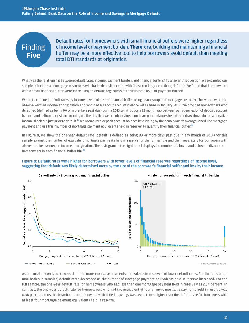
In Figure 8, we show the one-year default rate (default is defined as being 90 or more days past due in any month of 2014) for this

sample against the number of equivalent mortgage payments held in reserve for the full sample and then separately for borrowers with

above- and below-median income at origination. The histogram in the right panel displays the number of above- and below-median income

homeowners in each financial buffer bin.21

Figure 8: Default rates were higher for borrowers with lower levels of financial reserves regardless of income level, suggesting that default was likely determined more by the size of the borrower’s financial buffer and less by their income.

As one might expect, borrowers that held more mortgage payments equivalents in reserve had lower default rates. For the full sample

(and both sub samples) default rates decreased as the number of mortgage payment equivalents held in reserve increased. For the

full sample, the one-year default rate for homeowners who had less than one mortgage payment held in reserve was 2.54 percent. In

contrast, the one-year default rate for homeowners who had the equivalent of four or more mortgage payments held in reserve was

0.36 percent. Thus the default rate for borrowers with little in savings was seven times higher than the default rate for borrowers with

at least four mortgage payment equivalents held in reserve.


11

This result suggests that providing homeowners with an incentive to hold a financial

buffer of several mortgage payment equivalents could be a useful measure aimed

at preventing default. Furthermore, because almost half of homeowners had little

to no financial buffer (54 percent of this sample had fewer than four mortgage

payment equivalents held in reserve) and these homeowners have much higher

default rates (84 percent of total defaults are from homeowners with fewer

than four mortgage payment equivalents held in reserve), incenting these

homeowners to build a larger but still modest financial buffer could prevent

a large number of defaults. The marginal impact of each additional mortgage

payment held in reserve beyond four or five was small, which suggests that

only a relatively modest amount of savings could have a substantial impact on

default rates. In other words, the returns to incenting homeowners with very

little in reserve to save more could be very large.

The default rate for borrowers with little

savings was seven times higher than the default rate for borrowers

with at least four mortgage payment equivalents held in reserve, and 84 percent of total defaults were from homeowners with fewer than four

mortgage payment equivalents held in reserves.

A comparison of default rates for the above- and below-median income sub-samples

shown in Figure 8 indicates that, for borrowers with less than one mortgage payment

equivalent held in reserve, the default rate for the below-median income sample was 1.5

percentage points higher than the default rate for the above-median income sample. However,

for borrowers with at least one mortgage payment equivalent held in reserve, the difference in default rates

between the two sub-samples was considerably narrower (0.4 percentage points). This is particularly notable given the nearly $80,000

income gap between the average above-median income borrower and the average below-median income borrower. The fact that default

rates were similar for borrowers with more than one mortgage payment in reserve suggests that the lack of a financial buffer might have

been a more important determinant of mortgage default than income level.

An additional observation from Figure 8: within each income group, there was substantial variation in financial buffer size. In fact, the

histogram in the right panel shows that the proportion of borrowers in each bin was not that different across income groups, implying that

the correlation between income and savings was fairly weak. While one might have expected that higher income borrowers would make

up a larger proportion of observations as financial buffer increased, that was not evident in our data.22

As noted above, the data in Figure 8 suggest that it was the variation in financial buffers across borrowers within each income group

that determined default rate more so than the income level of a borrower—for the below-median income borrowers with less than one

mortgage payment in reserve, increasing their deposit account balance by the equivalent of one mortgage payment (moving along the line

to the right) had a greater impact on reducing the likelihood of default than increasing their income and moving into the above-median

income group (moving to the lower line). The average borrower in the below-median income group earned $42,000 per year. Practically

speaking, they would likely find it more feasible to save a few mortgage payments over time than to move to the above-median income

group (average income of $122,000 per year).


12

Next we investigated a commonly used metric of affordability in the mortgage underwriting process—total DTI at origination—and examined

how mortgage default rates varied for borrowers with different levels of total DTI at origination and financial buffers. Again, we began with

a sample of mortgage customers who had a deposit account with Chase and then subset this sample to those for whom we could observe

total DTI at origination. We found that homeowners with smaller balances in their deposit accounts were more likely to default regardless

of their total DTI at origination.

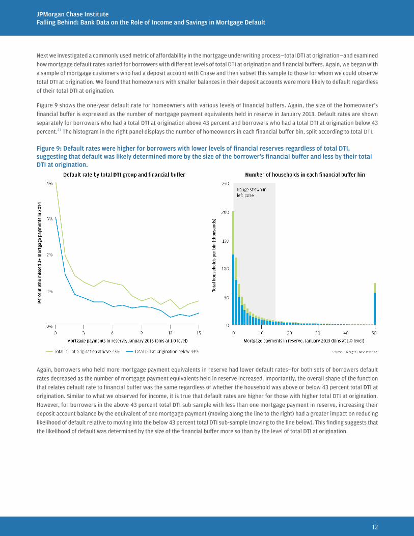
Figure 9 shows the one-year default rate for homeowners with various levels of financial buffers. Again, the size of the homeowner’s

financial buffer is expressed as the number of mortgage payment equivalents held in reserve in January 2013. Default rates are shown

separately for borrowers who had a total DTI at origination above 43 percent and borrowers who had a total DTI at origination below 43

percent.23 The histogram in the right panel displays the number of homeowners in each financial buffer bin, split according to total DTI.

Figure 9: Default rates were higher for borrowers with lower levels of financial reserves regardless of total DTI, suggesting that default was likely determined more by the size of the borrower’s financial buffer and less by their total DTI at origination.

Again, borrowers who held more mortgage payment equivalents in reserve had lower default rates—for both sets of borrowers default

rates decreased as the number of mortgage payment equivalents held in reserve increased. Importantly, the overall shape of the function

that relates default rate to financial buffer was the same regardless of whether the household was above or below 43 percent total DTI at

origination. Similar to what we observed for income, it is true that default rates are higher for those with higher total DTI at origination.

However, for borrowers in the above 43 percent total DTI sub-sample with less than one mortgage payment in reserve, increasing their

deposit account balance by the equivalent of one mortgage payment (moving along the line to the right) had a greater impact on reducing

likelihood of default relative to moving into the below 43 percent total DTI sub-sample (moving to the line below). This finding suggests that

the likelihood of default was determined by the size of the financial buffer more so than by the level of total DTI at origination.


13

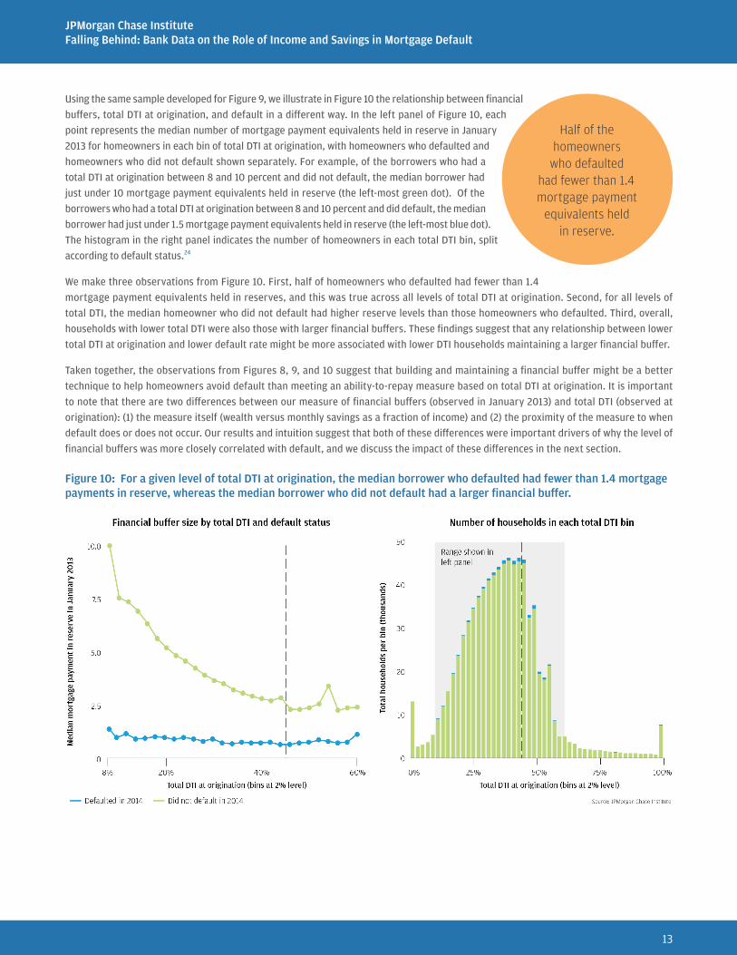
Using the same sample developed for Figure 9, we illustrate in Figure 10 the relationship between financial

buffers, total DTI at origination, and default in a different way. In the left panel of Figure 10, each

point represents the median number of mortgage payment equivalents held in reserve in January

2013 for homeowners in each bin of total DTI at origination, with homeowners who defaulted and

homeowners who did not default shown separately. For example, of the borrowers who had a

total DTI at origination between 8 and 10 percent and did not default, the median borrower had

just under 10 mortgage payment equivalents held in reserve (the left-most green dot). Of the

borrowers who had a total DTI at origination between 8 and 10 percent and did default, the median

borrower had just under 1.5 mortgage payment equivalents held in reserve (the left-most blue dot).

The histogram in the right panel indicates the number of homeowners in each total DTI bin, split

according to default status.24

Half of the homeowners

who defaulted had fewer than 1.4 mortgage payment

equivalents held in reserve.

We make three observations from Figure 10. First, half of homeowners who defaulted had fewer than 1.4

mortgage payment equivalents held in reserves, and this was true across all levels of total DTI at origination. Second, for all levels of

total DTI, the median homeowner who did not default had higher reserve levels than those homeowners who defaulted. Third, overall,

households with lower total DTI were also those with larger financial buffers. These findings suggest that any relationship between lower

total DTI at origination and lower default rate might be more associated with lower DTI households maintaining a larger financial buffer.

Taken together, the observations from Figures 8, 9, and 10 suggest that building and maintaining a financial buffer might be a better

technique to help homeowners avoid default than meeting an ability-to-repay measure based on total DTI at origination. It is important

to note that there are two differences between our measure of financial buffers (observed in January 2013) and total DTI (observed at

origination): (1) the measure itself (wealth versus monthly savings as a fraction of income) and (2) the proximity of the measure to when

default does or does not occur. Our results and intuition suggest that both of these differences were important drivers of why the level of

financial buffers was more closely correlated with default, and we discuss the impact of these differences in the next section.

Figure 10: For a given level of total DTI at origination, the median borrower who defaulted had fewer than 1.4 mortgage payments in reserve, whereas the median borrower who did not default had a larger financial buffer.


14

Implications From the preceding analyses, we draw implications for policy along

three dimensions: default prevention, helping homeowners facing a

negative income shock, and mortgage design.

Default prevention Establishing and maintaining a financial buffer was an important

component of avoiding default in the face of a negative income shock,

even for higher income homeowners. The default rate for borrowers with

less than the one mortgage payment equivalent held in reserve (2.54

percent) was seven times higher than the default rate for borrowers

with at least four mortgage payments in reserve (0.36 percent).

The public and private sector should consider ways to provide new

borrowers with an incentive to build and maintain a reserve fund

associated with their mortgage that could be drawn down in the face

of a negative income shock to avoid default. Designed carefully, such

a program could provide a method of reducing defaults that aligns

interests across the relevant mortgage stakeholders (borrower,

servicer, investor, GSEs, and insurer).

Previous research has shown that liquidity is a more important

determinant of default than debt level. As such, some lenders may want

to consider the trade-offs between down payment size and residual

cash reserves at origination. For example, a buyer who purchases a

$250,000 home and makes a 21 percent down payment but is left with

no savings may be more vulnerable to default compared to a buyer

who puts down 20.2 percent, has a monthly mortgage payment that is

$10 higher, and is left with the equivalent of 2 mortgage payments that

can be held as a financial buffer and used in the event of a temporary

negative income shock to avoid default.25 Paired with a reserve fund

as described above, some additional flexibility around down payment

and LTV limits at origination could lead to lower default rates.

A policy based on maintaining a minimum post-purchase financial

buffer may be a better approach to default prevention than

underwriting standards based on measuring the borrower’s static

ability-to-repay at origination. Meeting the ability-to-repay rule

requiring that a borrower’s total DTI at origination not exceed 43

percent to satisfy the Qualified Mortgage rule was not enough to

help borrowers faced with a negative income shock avoid default.

While total DTI measured at origination may have some predictive

power for default, the considerable heterogeneity in housing costs

and incomes makes it difficult to find a single level of total DTI that

indicates affordability across all households and regions. Research has

shown evidence that had the 43 percent total DTI limit been in effect

after 2004, it would have resulted in a minimal reduction in five-year

default rates for mortgages originated between 2005 and 2008. Thus

there is little evidence that potential homeowners just below the 43

percent total DTI threshold should be treated differently than potential

homeowners just above the 43 percent total DTI threshold.

A policy that provides

an economic incentive for borrowers to build and

maintain a financial buffer of a few mortgage payments

could be an effective default prevention

approach.

A financial buffer that is maintained through the early life of the

mortgage (when lower home equity levels leave homeowners who

face financial difficulty with fewer choices) may prove more effective

at avoiding default relative to meeting an ability-to-repay minimum

standard that is only observed at origination. Placing a limit on total

DTI as part of the underwriting process is inherently limited as a default

prevention tool precisely because (1) total DTI will likely change over

the life of the mortgage and (2) it creates no additional incentive for

the homeowner to build savings to counter a negative income shock. In

contrast, a policy that provides an economic incentive for borrowers to

build and maintain a financial buffer of a few mortgage payments could

be a more effective default prevention approach, precisely because the

reserves would be available in the event of a negative income shock.

Helping homeowners facing a negative income shockAs discussed in our previous research, mortgage modification programs

that aim to reduce default rates should focus on providing homeowners

who are struggling to make their monthly mortgage payments with

material payment reduction, regardless of their previous income level

or home equity. Furthermore, the amount of payment reduction should

not be predicated on reaching a predetermined affordability target.

The results in this brief further highlight the important connection

between a negative income shock and default and underscore the

importance of early intervention. By responding to missed mortgage

payments earlier, mortgage stakeholders and homeowners can together

estimate to the best of their ability the depth and potential duration of

their financial difficulty and arrive at a solution before arrearages build

and default ensues. Temporary forbearance could be used to mitigate

the impact of transitory income shocks, whereas more permanent

modifications may be appropriate for longer duration drops in income.

Considering the broad definition of income we used in our analysis,

there may be many reasons why a homeowner with a mortgage suffers

the type of negative income shock that we see associated with default,

including job loss, a reduction in hours within a job, or a loss of transfers.

For the homeowners who are experiencing a job loss, unemployment

insurance can act as a complement to traditional housing policy

programs. Research has shown that increasing unemployment benefits


https://cepr.org/sites/default/files/Johnson%2C%20Stephanie.pdf



15

after the Great Recession reduced mortgage defaults and foreclosures.

In contrast, the Federal programs designed to help homeowners with

a mortgage who were facing financial difficulty and/or negative equity

suffered from low take-up rates, suggesting these programs may have

been less impactful. Closer coordination between housing policymakers

and the federal and state policymakers charged with determining the

amount and duration of unemployment insurance benefits could better

ensure that the marginal tax dollar aimed at helping homeowners facing

a negative income shock avoid default is invested efficiently.

Research estimates that increases in unemployment insurance payment

amounts or duration helped avoid 1.3 million mortgage foreclosures

between 2008 and 2013 and therefore acted as an automatic stabilizer

for the housing market during this period.26 This result is consistent with

our findings regarding the impact of mortgage payment reductions on

default rates, and can be generalized—policies that either reduce monthly

payments or replace monthly income for homeowners struggling to make

their monthly mortgage payments will reduce subsequent default rates.

In contrast, the various federal programs implemented to help

unemployed or underemployed homeowners with a mortgage suffered

from relatively low subscription rates and therefore had a much smaller

impact on foreclosures. The Hardest Hit Fund (HHF) was established

in 2010 to help homeowners hit hardest by the economic and housing

market downturn and offered mortgage payment assistance for

unemployed or underemployed homeowners. By the end of 2016, only

292,000 homeowners had received assistance through the HHF. The

Home Affordable Unemployment Program (UP) was introduced in 2010

to provide assistance to homeowners who were unable to make their

mortgage payments as a result of unemployment. As of the end of

2016, only 46,485 homeowners were participating in the UP program.27

Similarly, the mortgage modification programs (e.g., the Home

Affordable Modification Program or HAMP) designed to aid homeowners

in the post-Great Recession period suffered from low uptake and had

a smaller impact on foreclosures. Between March 2009 and June 2010

about 55 percent (almost 675,000) of HAMP trial modifications were

cancelled because homeowners could not provide the requisite income

verification documentation. By April 2015, more than one million

homeowners had been denied a HAMP modification because they did

not provide the financial and/or hardship verification documentation

required to complete the evaluation of their request in a timely

manner.28 Research estimates that the HAMP program helped avoid

600,000 foreclosures between March 2009 and December 2012.

Research has also shown that the refinancing programs introduced

during the same period (e.g., the Home Affordable Refinance Program)

suffered from frictions that reduced their uptake to less than 50 percent

of eligible borrowers, and resulted in modest reductions to foreclosure

rates. Similarly, changing refinancing programs to require income

verification and upfront payment of closing costs reduced refinancing

rates by 50 percent.

While state-level unemployment insurance programs have varying

eligibility requirements, unemployment benefits directly target

households that would be ineligible for the various mortgage programs

that require income documentation.29 Unemployment insurance has the

added advantage relative to mortgage programs in that it offers relief to

homeowners that have lost a job without requiring input from mortgage

servicers, investors, various government agencies (e.g., FNMA, FHLMC,

FHA, etc.) or second lien holders. Taken together, these facts suggest that

unemployment insurance can act as a complement to traditional housing

policy programs to help homeowners facing a negative income shock.

Mortgage design Our analysis has implications for housing policymakers as they consider

the trade-offs between fixed-rate mortgages (FRMs) and adjustable-

rate mortgages (ARMs). The connection between negative income

shocks and default suggests that ARMs, which automatically adjust their

interest rates and monthly payments in accordance with the Federal

Reserve’s interest rate target range, can serve as a way to help stabilize

the economy during a recession.30 Additional empirical research is

needed to better understand the impact of ARMs on consumer spending

and default as policy rates normalize to higher levels.

As discussed in our previous research, accommodative monetary

policy is automatically transmitted to homeowners with ARMs, while

the transmission channel to homeowners with FRMs is harder to

activate and requires the borrower meet various pre-conditions that

limit its effectiveness. For borrowers with an FRM, this is true for

both the refinancing process and the mortgage modification process.

With respect to finding the optimal mortgage design, research suggests

that ARMs that include a feature that allows the borrower to reduce or

defer payments in the face of a negative income shock or during a recession

would reduce defaults and stabilize consumption across business cycles.

These ideas should be weighed in the broader context of providing

borrowers with mortgages that are simple and easy to understand.

Once armed with an assessment of the impact of ARMs on default and

consumption during an economic expansion, housing policymakers can

make the determination as to whether to consider the promotion and

standardization of ARMs for the appropriate set of borrowers (given

demographic and other characteristics).

Unemployment insurance can act

as a complement to traditional housing policy

programs aimed at homeowners facing

job loss.

https://www.aeaweb.org/articles?id=10.1257/aer.20140989


https://www.journals.uchicago.edu/doi/abs/10.1086/691701

https://chicagounbound.uchicago.edu/cgi/viewcontent.cgi?referer=http://www.google.com/url?sa=t&rct=j&q=&esrc=s&source=web&cd=1&ved=2ahUKEwiRtPuUh7bdAhWOl-AKHUlsD90QFjAAegQIABAC&url=http%3A%2F%2Fchicagounbound.uchicago.edu%2Fcgi%2Fviewcontent.cgi%3Farticle%3D1044%26context%3Dhousing_law_and_policy&usg=AOvVaw2hkv55oSRLjxvHnVWEZ3wo&httpsredir=1&article=1044&context=housing_law_and_policy

https://papers.ssrn.com/sol3/papers.cfm?abstract_id=3231596

https://www.jpmorganchase.com/corporate/institute/report-response-to-mortgage-resets.htm

https://www.jpmorganchase.com/corporate/institute/report-response-to-mortgage-resets.htm


http://people.bu.edu/guren/gkm_mortgage_design.pdf

https://papers.ssrn.com/sol3/papers.cfm?abstract_id=3135366


16

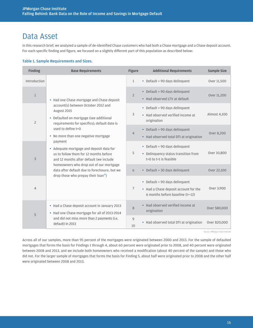
Data AssetIn this research brief, we analyzed a sample of de-identified Chase customers who had both a Chase mortgage and a Chase deposit account.

For each specific finding and figure, we focused on a slightly different part of this population as described below:

Table 1. Sample Requirements and Sizes.

Finding Base Requirements Figure Additional Requirements Sample Size

Introduction

• Had one Chase mortgage and Chase deposit

account(s) between October 2012 and

August 2015

• Defaulted on mortgage (see additional

requirements for specifics); default date is

used to define t=0

• No more than one negative mortgage

payment

• Adequate mortgage and deposit data for

us to follow them for 12 months before

and 12 months after default (we include

homeowners who drop out of our mortgage

data after default due to foreclosure, but we

drop those who prepay their loan31)

1 • Default = 90 days delinquent Over 11,500

1 2• Default = 90 days delinquent

• Had observed LTV at defaultOver 11,200

2

3

• Default = 90 days delinquent

• Had observed verified income at

origination

Almost 4,100

4• Default = 90 days delinquent

• Had observed total DTI at originationOver 8,200

3

5


• Delinquency status transition from

t=0 to t=1 is feasible

Over 10,800

6 • Default = 30 days delinquent Over 22,100

4 7


• Had a Chase deposit account for the

6 months before baseline (t=-12)

Over 3,900

5

• Had a Chase deposit account in January 2013

• Had one Chase mortgage for all of 2013-2014

and did not miss more than 2 payments (i.e.

default) in 2013

8• Had observed verified income at

originationOver 580,000

9• Had observed total DTI at origination Over 820,000

10

Source: JPMorgan Chase Institute

Across all of our samples, more than 95 percent of the mortgages were originated between 2000 and 2013. For the sample of defaulted

mortgages that forms the basis for Findings 1 through 4, about 60 percent were originated prior to 2008, and 40 percent were originated

between 2008 and 2013, and we include both homeowners who received a modification (about 40 percent of the sample) and those who

did not. For the larger sample of mortgages that forms the basis for Finding 5, about half were originated prior to 2008 and the other half

were originated between 2008 and 2013.


17

Endnotes

1 Our primary unit of analysis is the primary account holder (mortgage loan and Chase deposit account) and throughout this report, we will interchangeably use the terms “customers,” “accounts,” “homeowners,” and “households” to refer to this same concept.

2 About 60 percent of the mortgages in this sample were originated before 2008. The remaining 40 percent were originated between 2008 and 2013. For both groups, income dropped prior to default and the sizes of the drops in income and mortgage payment made were similar to each other.

3 Throughout this report we use a broad measure of income that includes all checking account inflows. As such, it combines labor and capital income, government support, and transfers from savings or retirement accounts, family members, and friends, etc. It includes inflows from all channels, including electronic transfers, paper check deposits, cash deposits, etc.

4 For this analysis, we defined default as a loan being 90 or more days past due. Note that not all borrowers were current at baseline (12 months before default), and therefore the cumulative amount of missed mortgage payments over the 12 months prior to default may not sum to three mortgage payments.

5 While we do not show the results, the relationship between income and mortgage payments made for homeowners who defaulted is robust to the definition of default. The pattern showing a drop in income followed by a drop in mortgage payment made a few months later was evident regardless of how we define default (e.g., 30, 60, 90, 120, 150 or 180 days delinquent).

6 The below 80 percent LTV group has over 5,400 Chase customers, the 80 to 100 percent group has almost 3,700 Chase customers, the 100 to 130 percent group has almost 1,700 Chase customers, and the over 130 percent group has over 400 Chase customers. Our mortgage default rates and LTV distributions closely match those from research based on a broader sample of mortgages.

7 Other research finds evidence of strategic default between 2006 and 2009 at LTVs above 174% for a set of nonprime borrowers originated in 2006 (the height of the house price boom) from Arizona, California, Florida, and Nevada with a CLTV at or above 100%. Our sample of borrowers is different—it was originated over more years and a broader set of states and has an LTV distribution more closely aligned with the broader set of mortgage holders and therefore few borrowers with an LTV above 160%. We examined default behavior between 2012 and 2015.

8 The ranges of monthly verified gross income at origination for each quartile are as follows: lowest income quartile (0, $3,089), second income quartile ($3,089, $4,596), third income quartile ($4,596, $6,728), and highest income quartile ($6,728, $12,189).

9 We conducted the same analysis of inflows and mortgage payment shown in Figure 3 using several alternative sources of income data to segment the sample into income quartiles, including estimated income based on Chase account activity and data, average monthly checking account inflows during the six months before baseline, and zip-code level income data from the IRS Statistics of Income. Using these alternate sources of income data, we observed the same patterns as shown in Figure 3.

10 As described in https://files.consumerfinance.gov/f/201301_cfpb_final-rule_ability-to-repay.pdf.

11 The below-43 percent total DTI group has almost 4,800 Chase customers and the above-43 percent group has over 3,500 Chase customers.

12 The total DTI calculation continues to evolve. For example, in 2017 Fannie Mae and Freddie Mac changed their policy with respect to student loan payments, as described in https://www.fanniemae.com/content/announcement/sel1706.pdf and http://www.freddiemac.com/singlefamily/guide/bulletins/pdf/bll1723.pdf.

13 Default is again defined as being 90 days past due. Borrowers who were less delinquent in the next month made the equivalent of two (or more) mortgage payments in the next month and became 60 (or fewer) days past due. Borrowers who were similarly delinquent in the next month made their next regularly scheduled payment, but did not make up their arrearages and remained 90 days past due. Borrowers who were more delinquent in the next month made no payment and became 120 days past due.

14 The Less Delinquent group includes almost 2,600 Chase customers, the Similarly Delinquent group contains over 2,600 Chase customers, and the More Delinquent group contains over 5,700 Chase customers.

15 The Current group includes over 6,700 Chase customers, the 30 days delinquent group contains over 7,200 Chase customers, the 60 to 90 days delinquent group contains over 3,900 Chase customers, the 120+ days delinquent group contains over 2,000 Chase customers, and the Foreclosure group contains over 2,100 Chase customers.

16 We also examined results similar to Figure 6 using various initial stages of delinquency (e.g., 60 days, 90 days, 120 days, and 150 days delinquent). In each case, homeowners who experienced deeper and longer negative income shocks became more delinquent in the month that followed, while those who experienced a recovery in income were able to resume making mortgage payments.

17 We require that customers have their Chase mortgage account for two years around default (t=-12 to t=12) and their Chase deposit account for two and a half years around default (t=-18 to t=12) (see Data Asset section) so that we can observe deposit account levels for six months before baseline (t=-12). We segment the customer into above-median and below-median deposit account groups based on their average checking plus savings account totals from t=-18 to t=-13 in order to reduce mean reversion in the results. In order to meet minimum aggregation standards, throughout this report medians are calculated as the average of the 11 observations closest to the median.

18 We normalize deposit account balances by dividing by the borrowers scheduled mortgage payment and express this as the number of mortgage payment equivalents held in reserve.

http://www.nber.org/papers/w21630

https://onlinelibrary.wiley.com/doi/abs/10.1111/jofi.12523

https://files.consumerfinance.gov/f/201301_cfpb_final-rule_ability-to-repay.pdf

https://files.consumerfinance.gov/f/201301_cfpb_final-rule_ability-to-repay.pdf

https://www.fanniemae.com/content/announcement/sel1706.pdf

https://www.fanniemae.com/content/announcement/sel1706.pdf

http://www.freddiemac.com/singlefamily/guide/bulletins/pdf/bll1723.pdf

http://www.freddiemac.com/singlefamily/guide/bulletins/pdf/bll1723.pdf


18

19 We also examined results by observing deposit account balances in January 2014 and found a similar relationship between default rates, income level, and deposit account balances as that shown in Figure 8.

20 The number of equivalent mortgage payments held in reserve = (average daily balance in checking account + average daily balance in savings account) / scheduled mortgage payment as observed in January 2013.

21 We truncate the x-axis of the left panel of Figure 8 at 15 mortgage payments in reserve as there are fewer customers in each bin beyond 15 mortgage payments and having a financial buffer of more than 15 mortgage payments had little to no impact on default rates.

22 It could be the case that the higher income borrowers in our sample are more likely to have liquid assets held outside of their Chase checking and savings accounts that we are unable to observe. However, that would likely mean that the curve for the above-median income group would shift closer to the curve for the below-median income group, which would imply that income had a smaller impact on default.

23 We truncate the x-axis of the left panel of Figure 9 at 15 mortgage payments in reserve as there are fewer customers in each bin beyond 15 mortgage payments and having a financial buffer of more than 15 mortgage payments had little to no impact on default rates.

24 We limit the x-axis in the left panel of Figure 10 to capture the vast majority of the observations shown in the histogram in the right panel. Specifically, we include observations where the total DTI at origination was between 8 percent and 60 percent, which covers 93 percent of our sample.

25 A $197,500 30-year fixed rate mortgage with a 4.55% interest rate has a monthly principal and interest payment of $1,007, whereas a $199,525 mortgage with a 4.55% interest rate has a monthly principal and interest payment of $1,017.

26 This is a partial equilibrium estimate calculated using constant layoff rates, mortgage leverage, and home values.

27 Source: Making Home Affordable Program Performance Report through the Fourth Quarter of 2016, https://www.treasury.gov/initiatives/financial-stability/reports/Documents/MHA%20Quarterly%20Report%20Q4%202016_C.pdf.

28 As noted in the SIGTARP July 29, 2015 Quarterly Report to Congress (see https://www.sigtarp.gov/Quarterly%20Reports/July_29_2015_Report_to_Congress.pdf) and the MHA Q4 2016 Performance Report (see https://www.treasury.gov/initiatives/financial-stability/reports/Documents/MHA%20Quarterly%20Report%20Q4%202016_C.pdf).

29 Research (see http://www.nber.org/papers/w10488 and https://ideas.repec.org/p/crd/wpaper/13001.html) shows that the take-up rates for unemployment insurance among the eligible unemployed vary between 63 and 83 percent.

30 This assumes that the ARM is beyond the fixed rate period and that the Federal Reserve lowers interest rates in response to the recession.

31 A robustness check of just those borrowers who prepaid their mortgage after defaulting showed a similar pattern whereby default closely followed a negative income shock of a similar magnitude.

https://www.treasury.gov/initiatives/financial-stability/reports/Documents/MHA%20Quarterly%20Report%20Q4%202016_C.pdf



https://www.sigtarp.gov/Quarterly%20Reports/July_29_2015_Report_to_Congress.pdf

https://www.sigtarp.gov/Quarterly%20Reports/July_29_2015_Report_to_Congress.pdf




http://www.nber.org/papers/w10488

https://ideas.repec.org/p/crd/wpaper/13001.html

https://ideas.repec.org/p/crd/wpaper/13001.html


19

AcknowledgementsWe thank our research team, specifically Yuan Chen, Annie Gao, and Melissa O’Brien for their hard work and contribution to this report.

We would also like to acknowledge the invaluable input of academic experts Michael Barr, Peter Ganong, and Pascal Noel, and

industry expert Michael Fratantoni from the Mortgage Bankers Association, all of whom provided thoughtful commentary, as well as

the contribution of other Institute researchers, including Chris Wheat, Amar Hamoudi, Chex Yu, Max Liebeskind, and Kerry Zhang. In

addition, we would like to thank Michael Weinbach and the Chase Mortgage Banking team for their support, especially Peter Muriungi,

Tina Shell, Bill Zaboski, Murdock Martin, and Andrew Lewis, as well as other experts within JPMorgan Chase, including Chris Henry,

Subra Subramanian, Matt Jozoff, and John Sim. We are deeply grateful for their generosity of time, insight, and support.

This effort would not have been possible without the critical support of our partners from the JPMorgan Chase Consumer & Community

Bank and Corporate Technology teams of data experts, including Samuel Assefa, Connie Chen, Anoop Deshpande, Senthilkumar Gurusamy,

Ram Mohanraj, Karen Narang, Stella Ng, Rob Rappa, Ashwin Sangtani, Michael Harasimowicz, and Anmol Karnad, and JPMorgan Chase

Institute team members Sruthi Rao, Kelly Benoit, Courtney Hacker, Jolie Spiegelman, Elizabeth Ellis, Maggie Tarasovitch, Carla Ricks,

Sarah Kuehl, Alyssa Flaschner, and Gena Stern.

Finally, we would like to acknowledge Jamie Dimon, CEO of JPMorgan Chase & Co., for his vision and leadership in establishing the Institute

and enabling the ongoing research agenda. Along with support from across the Firm—notably from Peter Scher, Max Neukirchen, Joyce

Chang, Patrik Ringstroem, Lori Beer, and Judy Miller—the Institute has had the resources and support to pioneer a new approach to

contribute to global economic analysis and insight.

Suggested CitationFarrell, Diana, Kanav Bhagat, and Chen Zhao. 2018. “Falling Behind: Bank Data on the Role of Income and Savings in Mortgage Default”

JPMorgan Chase Institute.

This material is a product of JPMorgan Chase Institute and is provided to you solely for general information purposes. Unless otherwise specifically stated, any views or opinions expressed herein are solely those of the authors listed, and may differ from the views and opinions expressed by J.P. Morgan Securities LLC (JPMS) Research Department or other departments or divisions of JPMorgan Chase & Co. or its affiliates. This material is not a product of the Research Department of JPMS. Information has been obtained from sources believed to be reliable, but JPMorgan Chase & Co. or its affiliates and/or subsidiaries (collectively J.P. Morgan) do not warrant its completeness or accuracy. Opinions and estimates constitute our judgment as of the date of this material and are subject to change without notice. The data relied on for this report are based on past transactions and may not be indicative of future results. The opinion herein should not be construed as an individual recommendation for any particular client and is not intended as recommendations of particular securities, financial instruments, or strategies for a particular client. This material does not constitute a solicitation or offer in any jurisdiction where such a solicitation is unlawful.

©2018 JPMorgan Chase & Co. All rights reserved. This publication or any portion hereof may not be reprinted, sold, or redistributed without the written consent of J.P. Morgan.