Embed Size (px)
Citation preview

Fall 2006 EE 5301 - VLSI Design Automation I III-1
EE 5301 – VLSI Design Automation IEE 5301 – VLSI Design Automation I
Kia Bazargan
University of Minnesota
Part III: PartitioningPart III: Partitioning
Fall 2006 EE 5301 - VLSI Design Automation I III-2
References and Copyright
• Textbooks referred (none required) [Mic94] G. De Micheli
“Synthesis and Optimization of Digital Circuits”McGraw-Hill, 1994.
[CLR90] T. H. Cormen, C. E. Leiserson, R. L. Rivest“Introduction to Algorithms”MIT Press, 1990.
[Sar96] M. Sarrafzadeh, C. K. Wong“An Introduction to VLSI Physical Design”McGraw-Hill, 1996.
[She99] N. Sherwani“Algorithms For VLSI Physical Design Automation”Kluwer Academic Publishers, 3rd edition, 1999.

Fall 2006 EE 5301 - VLSI Design Automation I III-3
References and Copyright (cont.)
• Slides used: (Modified by Kia when necessary) [©Sarrafzadeh] © Majid Sarrafzadeh, 2001;
Department of Computer Science, UCLA [©Sherwani] © Naveed A. Sherwani, 1992
(companion slides to [She99]) [©Keutzer] © Kurt Keutzer, Dept. of EECS,
UC-Berekeleyhttp://www-cad.eecs.berkeley.edu/~niraj/ee244/index.htm
[©Gupta] © Rajesh Gupta UC-Irvinehttp://www.ics.uci.edu/~rgupta/ics280.html
[©Kang] © Steve Kang UIUChttp://www.ece.uiuc.edu/ece482/
Fall 2006 EE 5301 - VLSI Design Automation I III-4
Partitioning
• Decomposition of a complex system into smaller subsystems Done hierarchically Partitioning done until each subsystem has
manageable size Each subsystem can be designed independently
• Interconnections between partitions minimized Less hassle interfacing the subsystems Communication between subsystems usually
costly
[©Sherwani]
Fall 2006 EE 5301 - VLSI Design Automation I III-5
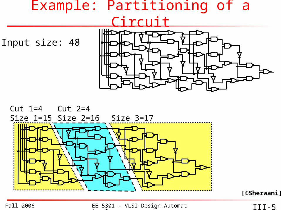
Example: Partitioning of a Circuit
[©Sherwani]
Input size: 48
Cut 1=4Size 1=15
Cut 2=4Size 2=16 Size 3=17
Fall 2006 EE 5301 - VLSI Design Automation I III-6
Hierarchical Partitioning
• Levels of partitioning: System-level partitioning:
Each sub-system can be designed as a single PCB
Board-level partitioning:Circuit assigned to a PCB is partitioned into sub-circuitseach fabricated as a VLSI chip
Chip-level partitioning:Circuit assigned to the chip is divided into manageable sub-circuitsNOTE: physically not necessary
[©Sherwani]

Fall 2006 EE 5301 - VLSI Design Automation I III-7
Delay at Different Levels of Partitions
AB
C
PCB1
[©Sherwani]
D
x
10x
20xPCB2

Fall 2006 EE 5301 - VLSI Design Automation I III-8
Partitioning: Formal Definition• Input:
Graph or hypergraph Usually with vertex weights (sizes) Usually weighted edges
• Constraints Number of partitions (K-way partitioning) Maximum capacity of each partition
ORmaximum allowable difference between partitions
• Objective Assign nodes to partitions subject to constraints
s.t. the cutsize is minimized
• Tractability Is NP-complete

Fall 2006 EE 5301 - VLSI Design Automation I III-9
Kernighan-Lin (KL) Algorithm• On non-weighted graphs• An iterative improvement technique• A two-way (bisection) partitioning algorithm• The partitions must be balanced (of equal
size)• Iterate as long as the cutsize improves:
Find a pair of vertices that result in the largest decrease in cutsize if exchanged
Exchange the two vertices (potential move) “Lock” the vertices If no improvement possible, and
still some vertices unlocked, thenexchange vertices that result in smallest increase in cutsizeW. Kernighan and S. Lin, Bell System Technical Journal, 1970.

Fall 2006 EE 5301 - VLSI Design Automation I III-10
Kernighan-Lin (KL) Algorithm• Initialize
Bipartition G into V1 and V2, s.t., |V1| = |V2| 1 n = |V|
• Repeat for i=1 to n/2
o Find a pair of unlocked vertices vai V1 and vbi V2 whoseexchange makes the largest decrease or smallest increasein cut-cost
o Mark vai and vbi as locked
o Store the gain gi.
Find k, s.t. i=1..k gi=Gaink is maximized If Gaink > 0 then
move va1,...,vak from V1 to V2 and vb1,...,vbk from V2 to V1.
• Until Gaink 0

Fall 2006 EE 5301 - VLSI Design Automation I III-11
Kernighan-Lin (KL) Example
a
b
c
d
e
f
g
h
4 { a, e } -2 5
0 -- 0 5
1 { d, g } 3 2
2 { c, f } 1 1
3 { b, h } -2 3
Step No. Vertex Pair Gain Cut-cost
[©Sarrafzadeh]

Fall 2006 EE 5301 - VLSI Design Automation I III-12
Kernighan-Lin (KL) : Analysis
Add “dummy” nodesReplace vertex of weight with vertices of size 1
• Time complexity? Inner (for) loop
o Iterates n/2 timeso Iteration 1: (n/2) x (n/2)o Iteration i: (n/2 – i + 1)2.
Passes? Usually independent of n O(n3)
• Drawbacks? Local optimum Balanced partitions only No weight for the vertices High time complexity Hyper-edges? Weighted edges?
Fall 2006 EE 5301 - VLSI Design Automation I III-13
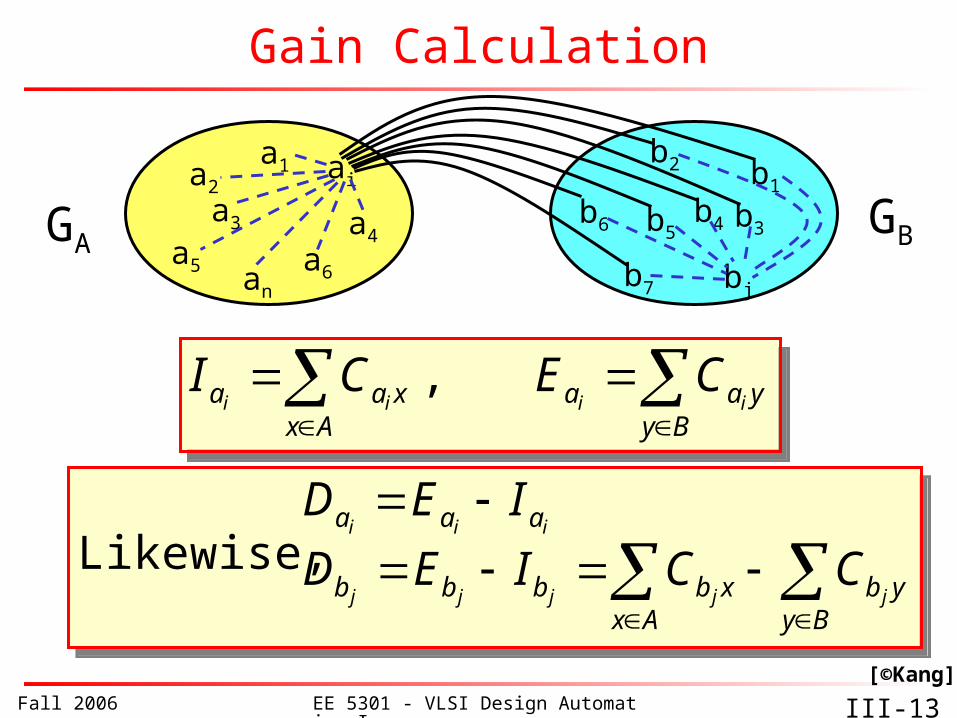
Internalcost
Gain Calculation
GAGB
a1a2
an
ai
a3
a5 a6
a4
b2
bj
b4 b3
b1
b6
b7
b5
Ax Byybxbbbb
aaa
jjjjj
iii
CCIED
IED Likewise,
Ax Byybxbbbb
aaa
jjjjj
iii
CCIED
IED Likewise,
[©Kang]
Externalcost
By
yaaAx
xaa iiiiCECI ,
By
yaaAx
xaa iiiiCECI ,

Fall 2006 EE 5301 - VLSI Design Automation I III-14
• Lemma: Consider any ai A, bj B.If ai, bj are interchanged, the gain is
• Proof: Total cost before interchange (T) between A and B
Total cost after interchange (T’) between A and B
Therefore
Gain Calculation (cont.)
jiji baba CDDg 2 jiji baba CDDg 2
[©Kang]
others) allfor cost (jiji baba CEET
others) allfor cost (jiji baba CIIT
jijjii babbaa CIEIETTg 2ia
Djb
D

Fall 2006 EE 5301 - VLSI Design Automation I III-15
Gain Calculation (cont.)• Lemma:
Let Dx’, Dy’ be the new D values for elements of A - {ai} and B - {bj}. Then after interchanging ai & bj,
• Proof: The edge x-ai changed from internal in Dx to external in Dx’
The edge y-bj changed from internal in Dx to external in Dx’
The x-bj edge changed from external to internal
The y-ai edge changed from external to internal
• More clarification in the next two slides
}{ , 22
}{ , 22
jyaybyy
ixbxaxx
bByCCDD
aAxCCDD
ij
ji
}{ , 22
}{ , 22
jyaybyy
ixbxaxx
bByCCDD
aAxCCDD
ij
ji
[©Kang]

Fall 2006 EE 5301 - VLSI Design Automation I III-16
Clarification of the Lemma
ai
bj
x

Fall 2006 EE 5301 - VLSI Design Automation I III-17
Clarification of the Lemma (cont.)• Decompose Ix and Ex to separate edges from ai and
bj:
• Write the equations before the move
• ... And after the move
ji xbxxax CECI
ji
ij
xbxa
xaxbxxx
CC
CCIED
)()(
ji
ji
xbxax
xbxax
CCD
CCD
22
ij xaxxbx CECI

Fall 2006 EE 5301 - VLSI Design Automation I III-18
Example: KL
• Step 1 - InitializationA = {2, 3, 4}, B = {1, 5, 6}A’ = A = {2, 3, 4}, B’ = B = {1, 5, 6}
• Step 2 - Compute D valuesD1 = E1 - I1 = 1-0 = +1
D2 = E2 - I2 = 1-2 = -1
D3 = E3 - I3 = 0-1 = -1
D4 = E4 - I4 = 2-1 = +1
D5 = E5 - I5 = 1-1 = +0
D6 = E6 - I6 = 1-1 = +0 [©Kang]
5
6
4 2 1
3
Initial partition
45
6 2
3
1

Fall 2006 EE 5301 - VLSI Design Automation I III-19
Example: KL (cont.) Step 3 - compute gains
g21 = D2 + D1 - 2C21 = (-1) + (+1) - 2(1) = -2
g25 = D2 + D5 - 2C25 = (-1) + (+0) - 2(0) = -1
g26 = D2 + D6 - 2C26 = (-1) + (+0) - 2(0) = -1
g31 = D3 + D1 - 2C31 = (-1) + (+1) - 2(0) = 0
g35 = D3 + D5 - 2C35 = (-1) + (0) - 2(0) = -1
g36 = D3 + D6 - 2C36 = (-1) + (0) - 2(0) = -1
g41 = D4 + D1 - 2C41 = (+1) + (+1) - 2(0) = +2
g45 = D4 + D5 - 2C45 = (+1) + (+0) - 2(+1) = -1
g46 = D4 + D6 - 2C46 = (+1) + (+0) - 2(+1) = -1
The largest g value is g41 = +2 interchange 4 and 1 (a1, b1) = (4, 1)
A’ = A’ - {4} = {2, 3}B’ = B’ - {1} = {5, 6} both not empty
[©Kang]

Fall 2006 EE 5301 - VLSI Design Automation I III-20
Example: KL (cont.)• Step 4 - update D values of node connected to vertices (4, 1)
D2’ = D2 + 2C24 - 2C21 = (-1) + 2(+1) - 2(+1) = -1D5’ = D5 + 2C51 - 2C54 = +0 + 2(0) - 2(+1) = -2D6’ = D6 + 2C61 - 2C64 = +0 + 2(0) - 2(+1) = -2
• Assign Di = Di’, repeat step 3 :g25 = D2 + D5 - 2C25 = -1 - 2 - 2(0) = -3g26 = D2 + D6 - 2C26 = -1 - 2 - 2(0) = -3g35 = D3 + D5 - 2C35 = -1 - 2 - 2(0) = -3g36 = D3 + D6 - 2C36 = -1 - 2 - 2(0) = -3
• All values are equal;arbitrarily choose g36 = -3 (a2, b2) = (3, 6)A’ = A’ - {3} = {2}, B’ = B’ - {6} = {5}
New D values are:D2’ = D2 + 2C23 - 2C26 = -1 + 2(1) - 2(0) = +1D5’ = D5 + 2C56 - 2C53 = -2 + 2(1) - 2(0) = +0
• New gain with D2 D2’, D5 D5’ g25 = D2 + D5 - 2C52 = +1 + 0 - 2(0) = +1 (a3, b3) = (2, 5)
[©Kang]
Fall 2006 EE 5301 - VLSI Design Automation I III-21
Example: KL (cont.)
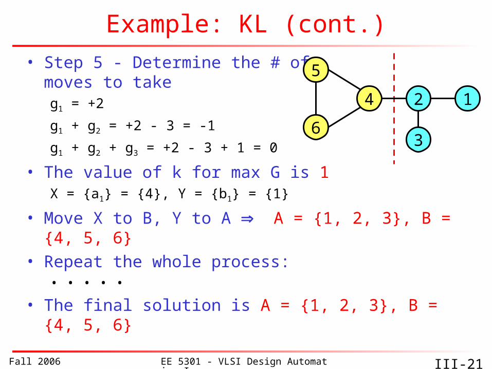
• Step 5 - Determine the # ofmoves to takeg1 = +2
g1 + g2 = +2 - 3 = -1
g1 + g2 + g3 = +2 - 3 + 1 = 0
• The value of k for max G is 1X = {a1} = {4}, Y = {b1} = {1}
• Move X to B, Y to A A = {1, 2, 3}, B = {4, 5, 6}• Repeat the whole process:
• • • • •
• The final solution is A = {1, 2, 3}, B = {4, 5, 6}
5
6
4 2 1
3

Fall 2006 EE 5301 - VLSI Design Automation I III-22
Fiduccia-Mattheyses (FM) Algorithm
• Modified version of KL• A single vertex is moved across the cut
in a single move Unbalanced partitions
• Vertices are weighted• Concept of cutsize extended to
hypergraphs• Special data structure to improve time
complexity to O(n2) (Main feature)
• Can be extended to multi-way partitioningC. M. Fiduccia and R. M. Mattheyses, 19th DAC, 1982.
Fall 2006 EE 5301 - VLSI Design Automation I III-23
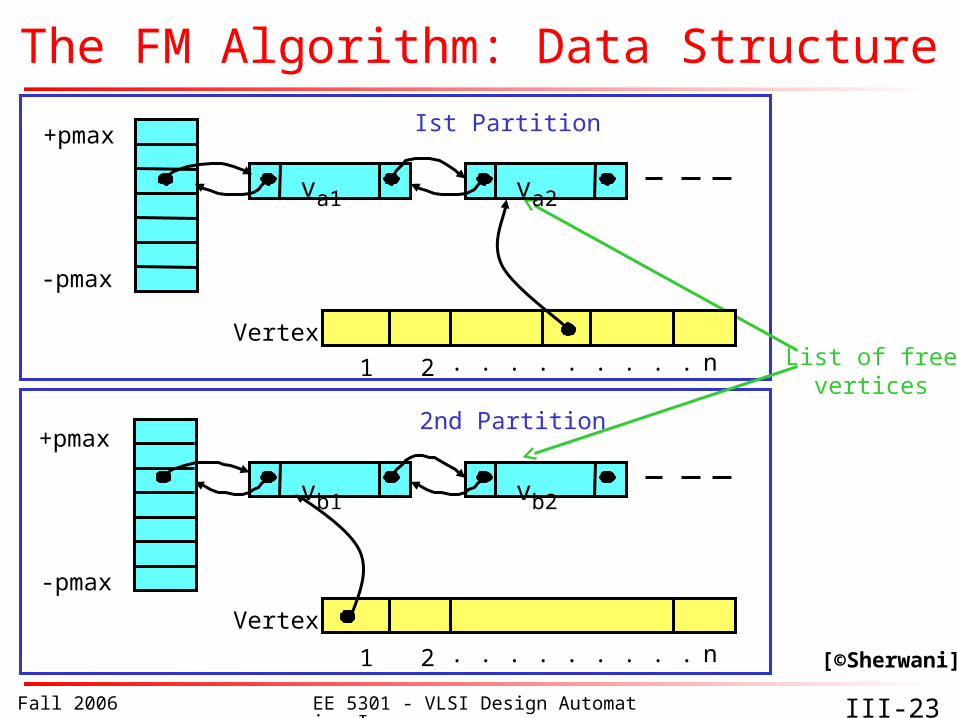
The FM Algorithm: Data Structure
-pmax
+pmax
+pmax
-pmax
2nd Partition
Ist Partition
List of freevertices
[©Sherwani]
va1 va2
vb1 vb2
Vertex
1 2 . . . . . . . . . n
Vertex
1 2 n. . . . . . . . .

Fall 2006 EE 5301 - VLSI Design Automation I III-24
The FM Algorithm: Data Structure• Pmax
Maximum gain pmax = dmax . wmax, where
dmax = max degree of a vertex (# edges incident to it)wmax is the maximum edge weight
What does it mean intuitively?
• -Pmax .. Pmax array Index i is a pointer to the list of unlocked vertices
with gain i.
• Limit on size of partition A maximum defined for the sum of vertex weights
in a partition(alternatively, the maximum ratio of partition sizes might be defined)
Fall 2006 EE 5301 - VLSI Design Automation I III-25
The FM Algorithm• Initialize
Start with a balance partition A, B of G(can be done by sorting vertex weights in decreasing order, placing them in A and B alternatively)
• Iterations Similar to KL A vertex cannot move if violates the balance
condition Choosing the node to move:
pick the max gain in the partitions Moves are tentative (similar to KL) When no moves possible or no more unlocked
vertices available, the pass ends When no move can be made in a pass, the algorithm
terminates

Fall 2006 EE 5301 - VLSI Design Automation I III-26
For multi terminal nets, K-L may decompose them into many 2-terminal nets, but not efficient!
Consider this example: If A = {1, 2, 3} B = {4, 5, 6}, graph model shows
the cutsize = 4 but in the real circuit, only 3 wires cut
Reducing the number of nets cut is more realistic than reducing the number of edges cut
Why Hyperedges?
[©Kang]
1
2
3
5
6
4
m
q
k
p
1
3
2
4
5
6
m
m
m
q
q
q
k
p
Fall 2006 EE 5301 - VLSI Design Automation I III-27
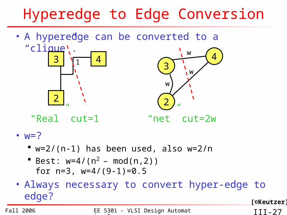
Hyperedge to Edge Conversion
• A hyperedge can be converted to a “clique”.
• w=? w=2/(n-1) has been used, also w=2/n Best: w=4/(n2 – mod(n,2))
for n=3, w=4/(9-1)=0.5
• Always necessary to convert hyper-edge to edge?
3
2
4
w
w
w
3 1
2
4
“Real” cut=1 “net” cut=2w
[©Keutzer]

Fall 2006 EE 5301 - VLSI Design Automation I III-28
FM Gain Calculation: Direct Hyperedge Calc
• FM is able to calculate gain directly using hyperedges ( not necessary to convert hyperedges to edges)
• Definition: Given a partition (A|B), we define the terminal
distribution of n as an ordered pair of integers (A(n),B(n)), which represents the number of cells net n has in blocks A and B respectively (how fast can be computed?)
Net is critical if there exists a cell on it such that if it were moved it would change the net’s cut state (whether it is cut or not).
Net is critical if A(n)=0,1 or B(n)=0,1[©Keutzer]

Fall 2006 EE 5301 - VLSI Design Automation I III-29
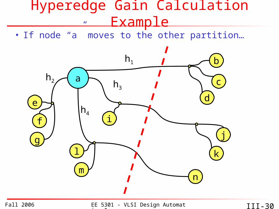
FM Gain Calc: Direct Hyperedge Calc (cont.)• Gain of cell depends only on its critical nets:
If a net is not critical, its cutstate cannot be affected by the move
A net which is not critical either before or after a move cannot influence the gains of its cells
• Let F be the “from” partition of cell i and T the “to”:
• g(i) = FS(i) - TE(i), where: FS(i) = # of nets which have cell i as their only F
cell TE(i) = # of nets connected to i and have an
empty T side
[©Keutzer]
Fall 2006 EE 5301 - VLSI Design Automation I III-30
Hyperedge Gain Calculation Example
• If node “a” moves to the other partition…
a
b
c
de
f
g
i
j
kl
mn
h1
h3
h2
h4

Fall 2006 EE 5301 - VLSI Design Automation I III-31
Subgraph Replication to Reduce Cutsize
• Vertices are replicated to improve cutsize• Good results if limited number of
components replicated
[©Sherwani]
A’
B’
A
B
A’A
BB’
C. Kring and A. R. Newta, ICCAD, 1991.

Fall 2006 EE 5301 - VLSI Design Automation I III-32
Clustering• Clustering
Bottom-up process Merge heavily connected
components into clusters Each cluster will be a new
“node” “Hide” internal connections (i.e.,
connecting nodes within a cluster)
“Merge” two edges incident to an external vertex, connecting it to two nodes in a cluster
• Can be a preprocessing step before partitioning Each cluster treated as a single
node
3
416
25
64
3
1
1
1
3
46
1,2
5
43
12
3,46
1,2
5
3
12
Fall 2006 EE 5301 - VLSI Design Automation I III-33
Other Partitioning Methods
• KL and FM have each held up very well• Min-cut / max-flow algorithms
Ford-Fulkerson – for unconstrained partitions
• Ratio cut• Genetic algorithm• Simulated annealing

Fall 2006 EE 5301 - VLSI Design Automation I III-34
To Probe Further...• B. Kernighan and S. Lin, "An Efficient Heuristic Procedure for
Partitioning of Electrical Circuits", Bell System Technical Journal", pp291-307, 1970.
• C. M. Fiduccia and R. M. Mattheyses. "A linear-time heuristic for improving network partitions“, Proceedings of the Design Automation Conference, pp 174-181, 1982.
• George Karypis, Rajat Aggarwal, Vipin Kumar and Shashi Shekhar, "Multilevel hypergraph partitioning: application in VLSI domain", Design Automation Conference, pp. 526-529, 1997.
• George Karypis and Vipin Kumar, "Multilevel k-way hypergraph partitioning", Design Automation Conference, pp. 343-348, 1999.
• A. E. Caldwell, A. B. Kahng and I. L. Markov, "Hypergraph Partitioning With Fixed Vertices", Design Automation Conference (DAC), pp. 355-359, 1999.
• A. E. Caldwell, A. B. Kahng, I. L. Markov, "Design and Implementation of Move-Based Heuristics for VLSI Hypergraph Partitioning", ACM Journal on Experimental Algorithms, Vol. 5, 2000.