WP/15/89

Fair Weather or Foul? The Macroeconomic Effects of El Niño

by Paul Cashin, Kamiar Mohaddes and Mehdi Raissi

© 2015 International Monetary Fund WP/15/89

IMF Working Paper

Asia and Pacific Department

Fair Weather or Foul? The Macroeconomic Effects of El Niño*1

Prepared by Paul Cashin, Kamiar Mohaddes** and Mehdi Raissi

Authorized for distribution by Paul Cashin

April 2015

Abstract

This paper employs a dynamic multi-country framework to analyze the international macroeconomic transmission of El Niño weather shocks. This framework comprises 21 country/region-specific models, estimated over the period 1979Q2 to 2013Q1, and accounts for not only direct exposures of countries to El Niño shocks but also indirect effects through third-markets. We contribute to the climate-macroeconomy literature by exploiting exogenous variation in El Niño weather events over time, and their impact on different regions cross-sectionally, to causatively identify the effects of El Niño shocks on growth, inflation, energy and non-fuel commodity prices. The results show that there are considerable heterogeneities in the responses of different countries to El Niño shocks. While Australia, Chile, Indonesia, India, Japan, New Zealand and South Africa face a short-lived fall in economic activity in response to an El Niño shock, for other countries (including the United States and European region), an El Niño occurrence has a growth-enhancing effect. Furthermore, most countries in our sample experience short-run inflationary pressures as both energy and non-fuel commodity prices increase. Given these findings, macroeconomic policy formulation should take into consideration the likelihood and effects of El Niño weather episodes.

JEL Classification Numbers: C32, F44, O13, Q54.

Keywords: El Niño weather shocks, oil and non-fuel commodity prices, global macroeconometric modeling, international business cycle.

Authors’ E-Mail Addresses: pcashin@imf.org; km418@cam.ac.uk; mraissi@imf.org.

* We are grateful to Tiago Cavalcanti, Hamid Davoodi, Govil Manoj, Rakesh Mohan, Sam Ouliaris, HashemPesaran, Vicki Plater, Ajay Shah, Ian South, Garima Vasishtha, Rick van der Ploeg, Yuan Yepez and seminar participants at the IMF's Asia and Pacific Department Discussion Forum, the IMF's Institute for Capacity Development, Oxford University, and the 13th Research Meeting of the National Institute of Public Finance and Policy and the Department of Economic Affairs of the Ministry of Finance in India for constructive comments and suggestions. The views expressed in this paper are those of the authors and do not necessarily represent those of the International Monetary Fund or IMF policy. ** Faculty of Economics and Girton College, University of Cambridge, United Kingdom.

This Working Paper should not be reported as representing the views of the IMF.

The views expressed in this Working Paper are those of the author(s) and do not necessarily represent those of the IMF or IMF policy. Working Papers describe research in progress by the author(s) and are published to elicit comments and to further debate.

2

Contents Page

I. Introduction . . . . . . . . . . . . . . . . . . . . . . . . . . . . . . . . . . . . . . . . . . . . . . . . . . . . . . . . . 3

II. The Southern Oscillation . . . . . . . . . . . . . . . . . . . . . . . . . . . . . . . . . . . . . . . . . . . . . . . 6

III. Modelling the Climate-Macroeconomy Relationship in a Global Context . . . . . . . . . 8 A. The Global VAR (GVAR) Methodology . . . . . . . . . . . . . . . . . . . . . . . . . . . . .9 B. Model Specification . . . . . . . . . . . . . . . . . . . . . . . . . . . . . . . . . . . . . . . . . . . . 12

IV. Empirical Results . . . . . . . . . . . . . . . . . . . . . . . . . . . . . . . . . . . . . . . . . . . . . . . . . . . . 14 A. The Effects of El Niño on Real Output . . . . . . . . . . . . . . . . . . . . . . . . . . . . . .16 B. The Effects of El Niño on Real Commodity Prices. .. . . . . . . . . . . . . . . . . . . 21 C. The Effects of El Niño on Inflation . . . . . . . . . . . . . . . . . . . . . . . . . . . . . . . . 22 D. Robustness Checks . . . . . . . . . . . . . . . . . . . . . . . . . . . . . . . . . . . . . . . . . . . . . 25

V. Concluding Remarks . . . . . . . . . . . . . . . . . . . . . . . . . . . . . . . . . . . . . . . . . . . . . . . . . 25

References . . . . . . . . . . . . . . . . . . . . . . . . . . . . . . . . . . . . . . . . . . . . . . . . . . . . . . . . . . . . . . . 27

Tables 1. Countries and Regions in the GVAR Model . . . . . . . . . . . . . . . . . . . . . . . . . . . . . . . 12 2. Lag Orders of the Country-Specific VARX*(p,q) Models Together with the Number

of Cointegrating Relations (r) . . . . . . . . . . . . . . . . . . . . . . . . . . . . . . . . . . . . . . . . . . .15 3. The Effects of an El Niño Shock on Real GDP Growth (in percent) . . . . . . . . . . . . .17 4. Share of Primary Sector in GDP (in percent), Averages over 2004-2013 . . . . . . . . . 17 5. Trade Weights, Averages over 2009–2011 . . . . . . . . . . . . . . . . . . . . . . . . . . . . . . . . 20 6. The Effects of an El Niño Shock on Real Commodity Prices (in percent) . . . . . . . . .22 7. The Effects of an El Niño Shock on Inflation (in percent). . . . . . . . . . . . . . . . . . . . . 24

Figures 1. Growth and Inflation Following the 1997/98 El Niño Episode . . . . . . . . . . . . . . . . . . 4 2. Southern Oscillation . . . . . . . . . . . . . . . . . . . . . . . . . . . . . . . . . . . . . . . . . . . . . . . . . . . 7 3. Global Climatological Effects of El Nino . . . . . . . . . . . . . . . . . . . . . . . . . . . . . . . . . . .7 4. Southern Oscillation Index (Anomalies), 1979M4–2014M12 . . . . . . . . . . . . . . . . . . .7 5. Food Weight in CPI Basket and Inflation Responses . . . . . . . . . . . . . . . . . . . . . . . . .24

3

I. INTRODUCTION

A rapidly growing literature investigates the relationship between climate (temperature,

precipitation, storms, and other aspects of the weather) and economic performance

(agricultural production, labor productivity, commodity prices, health, conflict, and economic

growth)—see the recent surveys by Dell et al. (2014) and Tol (2009). This is important as a

careful understanding of the climate-economy relationship is essential to the effective design

of appropriate institutions and macroeconomic policies, as well as enabling forecasts of how

future changes in climate will affect economic activity. However, a key challenge in studying

such a relationship is "identification", i.e. distinguishing the effects of climate on economic

activity from many other characteristics potentially covarying with it. We contribute to the

climate-economy literature by exploiting the exogenous variation in weather-related events

(with a special focus on El Niño1) over time, and their impact on different regions

cross-sectionally, to causatively identify the effects of El Niño weather shocks on growth,

inflation, energy and non-fuel commodity prices within a compact model of the global

economy.

Our focus on El Niño weather events is motivated by growing concerns about their effects not

only on the global climate system, but also on commodity prices and the macroeconomy of

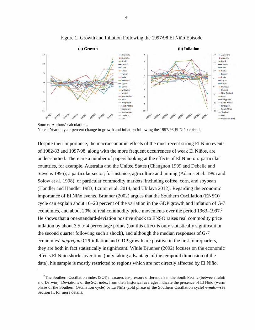
different countries—see Figure 1 for the evolution of growth and inflation across countries

following the most recent strong El Niño episode which started in 1997Q2 and ended in

1998Q1. These extreme weather conditions can constrain the supply of rain-driven

agricultural commodities, create food-price and generalized inflation, and may trigger social

unrest in commodity-dependent countries that primarily rely on imported food. It has been

suggested, by both historians and economists, that El Niño shocks may even have played a

role in a substantial number of civil conflicts, see Hsiang et al. (2011). To analyze the

macroeconomic transmission of El Niño shocks, both nationally and internationally, we

employ a dynamic multi-country framework (combining time series, panel data, and factor

analysis techniques), which takes into account economic interlinkages and spillovers that exist

between different regions. It also controls for macroeconomic determinants of energy and

non-fuel commodity prices, thereby disentangling the El Niño shock from many other

possible sources of omitted variable bias. This is crucial, given the global dimension of

commodity-price dynamics, and the interrelated macroeconomic performance of most

countries.

1El Niño is a band of above-average ocean surface temperatures that periodically develops off the Pacific coast

of South America, and causes major climatological changes around the world.

4

Figure 1. Growth and Inflation Following the 1997/98 El Niño Episode

(a) Growth (b) Inflation

Source: Authors’ calculations.

Notes: Year on year percent change in growth and inflation following the 1997/98 El Niño episode.

Despite their importance, the macroeconomic effects of the most recent strong El Niño events

of 1982/83 and 1997/98, along with the more frequent occurrences of weak El Niños, are

under-studied. There are a number of papers looking at the effects of El Niño on: particular

countries, for example, Australia and the United States (Changnon 1999 and Debelle and

Stevens 1995); a particular sector, for instance, agriculture and mining (Adams et al. 1995 and

Solow et al. 1998); or particular commodity markets, including coffee, corn, and soybean

(Handler and Handler 1983, Iizumi et al. 2014, and Ubilava 2012). Regarding the economic

importance of El Niño events, Brunner (2002) argues that the Southern Oscillation (ENSO)

cycle can explain about 10–20 percent of the variation in the GDP growth and inflation of G-7

economies, and about 20% of real commodity price movements over the period 1963–1997.2

He shows that a one-standard-deviation positive shock to ENSO raises real commodity price

inflation by about 3.5 to 4 percentage points (but this effect is only statistically significant in

the second quarter following such a shock), and although the median responses of G-7

economies’ aggregate CPI inflation and GDP growth are positive in the first four quarters,

they are both in fact statistically insignificant. While Brunner (2002) focuses on the economic

effects El Niño shocks over time (only taking advantage of the temporal dimension of the

data), his sample is mostly restricted to regions which are not directly affected by El Niño.

2The Southern Oscillation index (SOI) measures air-pressure differentials in the South Pacific (between Tahiti

and Darwin). Deviations of the SOI index from their historical averages indicate the presence of El Niño (warm

phase of the Southern Oscillation cycle) or La Niña (cold phase of the Southern Oscillation cycle) events—see

Section II. for more details.

5

We contribute to the literature that assesses the macroeconomic effects of weather shocks in

several dimensions, including a novel multi-country methodology. Our modelling framework

accounts for the effects of common factors (whether observed or unobserved), and ensures

that the El Niño-economy relationship is identified from idiosyncratic local characteristics

(using both time-series and cross-section dimensions of the data). To the extent that El Niño

events are exogenously determined, reverse causation is unlikely to be a concern in our

empirical analysis. Nevertheless, we allow for a range of endogenous control regressors,

where country-specific variables are affected by El Niño shocks and possibly simultaneously

determined by other observed or unobserved factors. We also have a different macroeconomic

emphasis—while Brunner (2002) mainly focuses on the effects of El Niño on commodity

prices, we concentrate on the implications of El Niño for national economic growth and

inflation, in addition to global energy and non-fuel commodity prices. Moreover, we study the

effects of El Niño shocks on 21 individual countries/regions (some of which are directly

affected by El Niño) in an interlinked and compact model of the world economy, rather than

focusing on an aggregate measure of global growth and inflation (which Brunner 2002 takes

to be those of G-7 economies). Furthermore, we explicitly take into account the economic

interlinkages and spillovers that exist between different regions in our interconnected

framework (which may also shape the responses of different macroeconomic variables to El

Niño shocks), rather than undertaking a country-by-country analysis. Finally, we contribute to

the Global VAR (GVAR) literature that mostly relies on reduced-form impulse-response

analysis by introducing El Niño as a dominant and causal variable in our framework.

Our framework comprises 21 country/region-specific models, among which is a single

European region. These individual-economy models are solved in a global setting where core

macroeconomic variables of each economy are related to corresponding foreign variables and

a set of global factors—including a measure of El Niño intensity as a dominant unit. The

model has the following variables: real GDP, inflation, real exchange rate, short-term and

long-term interest rates, real energy and non-fuel commodity prices, and the Southern

Oscillation index (SOI) anomalies as a measure of the magnitude of El Niño. This framework

accounts for not only direct exposures of countries to El Niño shocks but also indirect effects

through third-markets; see Dees et al. (2007) and Pesaran et al. (2007). We estimate the 21

individual VARX* models over the period 1979Q2–2013Q1. Having solved the Global VAR

model, we examine the effect of El Niño shocks on the macroeconomic variables of different

countries (especially those that are most susceptible to this weather phenomenon).3

3The GVAR methodology is a novel approach to global macroeconomic modeling as it combines time series,

panel data, and factor analysis techniques to address the curse of dimensionality problem in large models, and is

6

Contrary to the findings of earlier studies, the results of our dynamic multi-country model of

the world economy indicate that the economic consequences of El Niño shocks are large,

statistically significant, and highly heterogeneous across different regions. While Australia,

Chile, Indonesia, India, Japan, New Zealand and South Africa face a short-lived fall in

economic activity in response to a typical El Niño shock, for other countries, an El Niño event

has a growth-enhancing effect; some (for instance the United States) due to direct effects

while others (for instance the European region) through positive spillovers from major trading

partners.4 Overall, the larger the geographical area of a country, the smaller the primary

sector’s share in national GDP, and the more diversified the economy is, the smaller is the

impact of El Niño shocks on GDP growth. Furthermore, most countries in our sample

experience short-run inflationary pressures following an El Niño shock (depending mainly on

the share of food in their CPI baskets), while global energy and non-fuel commodity prices

increase. Therefore, we argue that macroeconomic policy formulation should take into

consideration the likelihood and effects of El Niño weather episodes.

The rest of the paper is organized as follows. Section II. gives a brief description of the

Southern Oscillation cycle. Section III. describes the GVAR methodology and outlines our

modelling approach. Section IV. investigates the macroeconomic effects of El Niño shocks.

Finally, Section V. concludes and offers some policy recommendations.

II. THE SOUTHERN OSCILLATION

During "normal" years, a surface high pressure system develops over the coast of Peru and a

low pressure system builds up in northern Australia and Indonesia (see Figure 2a). As a result,

trade winds move strongly from east to west over the Pacific Ocean. These trade winds carry

warm surface waters westward and bring precipitation to Indonesia and Australia. Along the

coast of Peru, cold nutrient-rich water wells up to the surface, and thereby boosts the fishing

industry in South America.

However, in an El Niño year, air pressure drops along the coast of South America and over

large areas of the central Pacific. The "normal" low pressure system in the western Pacific

also becomes a weak high pressure system, causing the trade winds to be reduced and

able to account for spillovers and the effects of ubserved and unobserved common factors (e.g. commodity-price

shocks and global finacial cycle)—see Section III.A. for additional details.

4Changnon (1999) also argues that an El Niño event can benefit the economy of the United States on a net

basis—amounting to 0.2% of GDP during the 1997/98 period.

7

Figure 2. Southern Oscillation

(a) Southern Oscillation (b) El Niño Conditions

Source: Pidwirny (2006).

Figure 3. Global Climatological Effects of El Nino

Source: National Atmospheric and Oceanic Administration’s (NOAA) Climate Prediction Center.

Figure 4. Southern Oscillation Index (Anomalies), 1979M4–2014M12

(a) SOI (b) SOI Anomalies

Source: Authors’ construction based on data from the Australian Bureau of Meteorology and the U.S. National

Oceanic and Atmospheric Administration’s National Climatic Data Centre.

Notes: Dashed-lines indicate thresholds for identifying El Niño and La Niña events.

8

allowing the equatorial counter current (which flows west to east) to accumulate warm ocean

water along the coastlines of Peru (Figure 2b). This phenomenon causes the thermocline (the

separation zone between the mixed-layer above, much influenced by atmospheric fluxes, and

the deep ocean) to drop in the eastern part of Pacific Ocean, cutting off the upwelling of cold

deep ocean water along the coast of Peru. Overall, the development of an El Niño brings

drought to the western Pacific (including Australia), rains to the equatorial coast of South

America, and convective storms and hurricanes to the central Pacific. The global

climatological effects of El Niño are summarized in Figure 3, showing the effects across two

different seasons. These changes in weather patterns have significant effects on agriculture,

fishing, and construction industries, as well as on national and global commodity prices.

Moreover, due to linkages of the Southern Oscillation with other climatic oscillations around

the world, El Niño effects reach far beyond the realm of the Pacific Ocean region.5

One of the ways of measuring El Niño intensity is by using the Southern Oscillation index

(SOI), which is calculated based on air-pressure differentials in the South Pacific (between

Tahiti and Darwin). Sustained negative SOI values below -8 indicate El Niño episodes, which

typically occur at intervals of three to seven years and last about two years. Figure 4 shows

that the 1982–83 and 1997–98 El Niños were quite severe (and had large adverse

macroeconomic effects in many regions of the world), whereas other El Niños in our sample

period were relatively moderate: 1986-88, 1991-92, 1993, 1994-95, 2002-03, 2006-07, and

2009-10. SOI "anomalies", which we use in our model, are defined as the deviation of the SOI

index from their historical averages and divided by their historical standard deviations.

Sustained negative SOI anomaly values below -1 indicate El Niño episodes (Figure 4b).

III. MODELLING THE CLIMATE-MACROECONOMY RELATIONSHIP IN A GLOBAL

CONTEXT

We employ the Global VAR (GVAR) methodology to analyze the international

macroeconomic transmission of El Niño shocks. This framework takes into account both the

temporal and cross-sectional dimensions of the data; real and financial drivers of economic

activity; interlinkages and spillovers that exist between different regions; and the effects of

unobserved or observed common factors (e.g. energy and non-fuel commodity prices). This is

crucial as the impact of El Niño shocks cannot be reduced to one country but rather involve

5La Niña weather events (cold phases of the Southern Oscillation cycle) produce the opposite climate varia-

tions from El Niño occurances. Since the effects of La Niña on fisheries along the coast of South America, where

El Niño was named, are benign, they received relatively little attention.

9

multiple regions, and may be amplified or dampened depending on the degree of openness of

the countries and their trade structure. Before describing the data and our model specification,

we provide a short exposition of the GVAR methodology below.

A. The Global VAR (GVAR) Methodology

We consider N + 1 countries in the global economy, indexed by i = 0, 1, ..., N . With the

exception of the United States, which we label as 0 and take to be the reference country; all

other N countries are modelled as small open economies. This set of individual VARX*

models is used to build the GVAR framework. Following Pesaran (2004) and Dees et al.

(2007), a VARX* (pi, qi) model for the ith country relates a ki × 1 vector of domestic

macroeconomic variables (treated as endogenous), xit, to a k∗i × 1 vector of country-specific

foreign variables (taken to be weakly exogenous), x∗it:

Φi (L, pi)xit = ai0 + ai1t+Λi (L, qi)x∗it + uit, (1)

for t = 1, 2, ..., T , where ai0 and ai1 are ki × 1 vectors of fixed intercepts and coefficients on

the deterministic time trends, respectively, and uit is a ki × 1 vector of country-specific

shocks, which we assume are serially uncorrelated with zero mean and a non-singular

covariance matrix, Σii, namely uit ∼ i.i.d. (0,Σii). For algebraic simplicity, we abstract from

observed global factors in the country-specific VARX* models. Furthermore,

Φi (L, pi) = I −∑pi

i=1 ΦiLi and Λi (L, qi) =

∑qii=0 ΛiL

i are the matrix lag polynomial of the

coefficients associated with the domestic and foreign variables, respectively. As the lag orders

for these variables, pi and qi, are selected on a country-by-country basis, we are explicitly

allowing for Φi (L, pi) and Λi (L, qi) to differ across countries.

The country-specific foreign variables are constructed as cross-sectional averages of the

domestic variables using data on bilateral trade as the weights, wij:

x∗it =N∑j=0

wijxjt, (2)

where j = 0, 1, ...N, wii = 0, and∑N

j=0wij = 1. For empirical application, the trade weights

10

are computed as three-year averages:6

wij =Tij,2009 + Tij,2010 + Tij,2011Ti,2009 + Ti,2010 + Ti,2011

, (3)

where Tijt is the bilateral trade of country i with country j during a given year t and is

calculated as the average of exports and imports of country i with j, and Tit =∑N

j=0 Tijt (the

total trade of country i) for t = 2009, 2010 and 2011, in the case of all countries.

Although estimation is done on a country-by-country basis, the GVAR model is solved for the

world as a whole, taking account of the fact that all variables are endogenous to the system as

a whole. After estimating each country VARX*(pi, qi) model separately, all the k =∑N

i=0 ki

endogenous variables, collected in the k × 1 vector xt = (x′0t,x

′1t, ...,x

′Nt)′, need to be solved

simultaneously using the link matrix defined in terms of the country-specific weights. To see

this, we can write the VARX* model in equation (1) more compactly as:

Ai (L, pi, qi) zit = ϕit, (4)

for i = 0, 1, ..., N, where

Ai (L, pi, qi) = [Φi (L, pi)−Λi (L, qi)] , zit = (x′it,x

′∗it)′,

ϕit = ai0 + ai1t+ uit. (5)

Note that given equation (2) we can write:

zit = Wixt, (6)

where Wi = (Wi0,Wi1, ...,WiN), with Wii = 0, is the (ki + k∗i )× k weight matrix for

country i defined by the country-specific weights, wij . Using (6) we can write (4) as:

Ai (L, p)Wixt = ϕit, (7)

where Ai (L, p) is constructed from Ai (L, pi, qi) by setting

p = max (p0, p1, ..., pN , q0, q1, ..., qN) and augmenting the p− pi or p− qi additional terms in

the power of the lag operator by zeros. Stacking equation (7), we obtain the Global VAR(p)

6The main justification for using bilateral trade weights, as opposed to financial weights, is that the former

have been shown to be the most important determinant of national business cycle comovements (see Baxter and

Kouparitsas (2005)).

11

model in domestic variables only:

G (L, p)xt = ϕt, (8)

where

G (L, p) =

A0 (L, p)W0

A1 (L, p)W1

.

.

.

AN (L, p)WN

, ϕt =

ϕ0t

ϕ1t

.

.

.

ϕNt

. (9)

For an early illustration of the solution of the GVAR model, using a VARX*(1, 1) model, see

Pesaran (2004), and for an extensive survey of the latest developments in GVAR modeling,

both the theoretical foundations of the approach and its numerous empirical applications, see

Chudik and Pesaran (2014). The GVAR(p) model in equation (8) can be solved recursively

and used for a number of purposes, such as forecasting or impulse response analysis.

Chudik and Pesaran (2013) extend the GVAR methodology to a case in which common

variables are added to the conditional country models (either as observed global factors or as

dominant variables). In such circumstances, equation (1) should be augmented by a vector of

dominant variables, ωt, and its lag values:

Φi (L, pi)xit = ai0 + ai1t+Λi (L, qi)x∗it +Υi (L, si)ωt + uit, (10)

where Υi (L, si) =∑si

i=0 ΥiLi is the matrix lag polynomial of the coefficients associated

with the common variables. Here, ωt can be treated (and tested) as weakly exogenous for the

purpose of estimation. The marginal model for the dominant variables can be estimated with

or without feedback effects from xt. To allow for feedback effects from the variables in the

GVAR model to the dominant variables via cross-section averages, we define the following

model for ωt:

ωt =

pw∑l=1

Φωlωi,t−l +

pw∑l=1

Λωlx∗i,t−l + ηωt (11)

It should be noted that contemporaneous values of star variables do not feature in equation

(11) and ωt are "causal". Conditional (10) and marginal models (11) can be combined and

12

solved as a complete GVAR model as explained earlier.

B. Model Specification

Key countries in our sample include those likely to be directly affected by El Niño—mainly

countries in the Asia and Pacific region as well as those in the Americas, see Table 1 and

Section II.. To investigate the possible indirect effects of El Niño (through trade, commodity

price and financial channels), we also include other major economies, such as European

countries, in the model. However, the main focus of the present study is not Europe, given

that it is not likely to be directly affected by an El Niño shock. Therefore, for this empirical

application, we create a region consisting of 13 European countries. The time series data for

the Europe block are constructed as cross-sectionally weighted averages of the domestic

variables, using Purchasing Power Parity GDP weights, averaged over the 2009-2011 period.

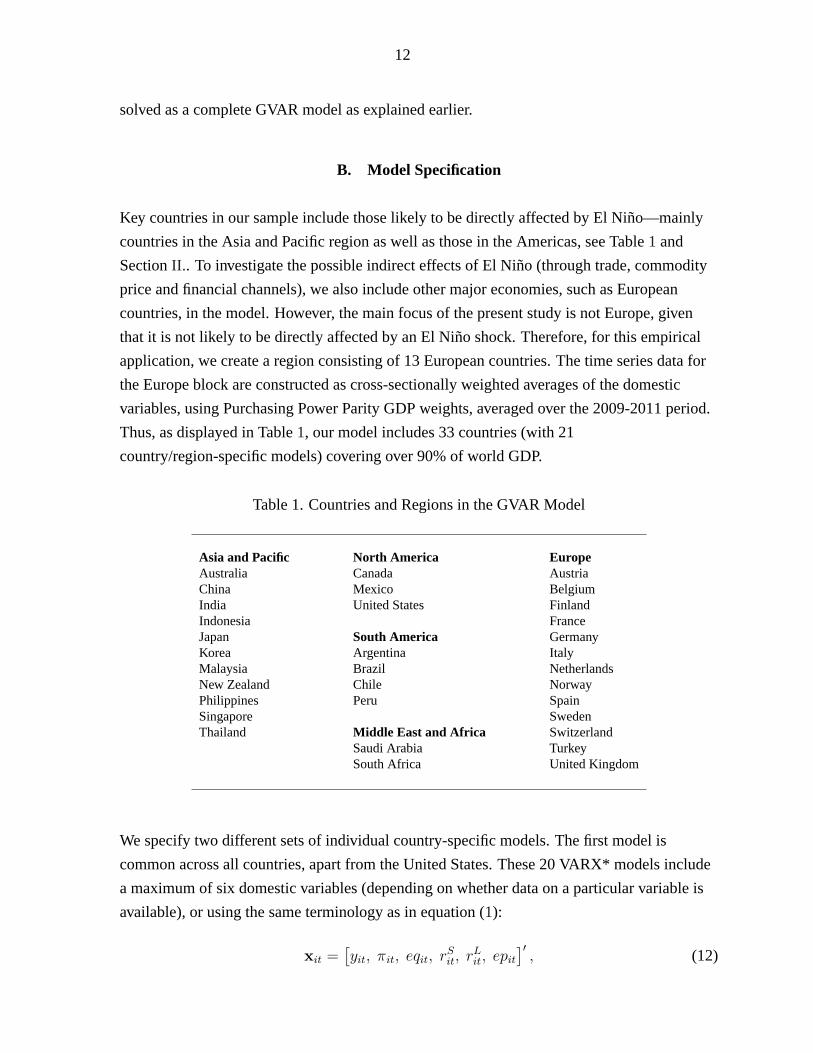
Thus, as displayed in Table 1, our model includes 33 countries (with 21

country/region-specific models) covering over 90% of world GDP.

Table 1. Countries and Regions in the GVAR Model

Asia and Pacific North America Europe

Australia Canada Austria

China Mexico Belgium

India United States Finland

Indonesia France

Japan South America Germany

Korea Argentina Italy

Malaysia Brazil Netherlands

New Zealand Chile Norway

Philippines Peru Spain

Singapore Sweden

Thailand Middle East and Africa Switzerland

Saudi Arabia Turkey

South Africa United Kingdom

We specify two different sets of individual country-specific models. The first model is

common across all countries, apart from the United States. These 20 VARX* models include

a maximum of six domestic variables (depending on whether data on a particular variable is

available), or using the same terminology as in equation (1):

xit =[yit, πit, eqit, r

Sit, r

Lit, epit

]′, (12)

13

where yit is the log of the real Gross Domestic Product at time t for country i, πit is inflation,

eqit is the log of real equity prices, rSit (rLit) is the short (long) term interest rate, and epit is the

real exchange rate. In addition, all domestic variables, except for that of the real exchange

rate, have corresponding foreign variables computed as in equation (2):

x∗it =[y∗it, π

∗it, eq

∗it, r

∗Sit , r

∗Lit

]′. (13)

Following the GVAR literature, the twenty-first model (United States) is specified differently,

mainly because of the dominance of the United States in the world economy. First, given the

importance of U.S. financial variables in the global economy, the U.S.-specific foreign

financial variables, eq∗US,t, r∗SUS,t, and r∗LUS,t, are not included in this model. The appropriateness

of exclusion of these variables was also confirmed by statistical tests, in which the weak

exogeneity assumption was rejected for eq∗US,t, r∗SUS,t, and r∗LUS,t. Second, since eit is expressed

as the domestic currency price of a United States dollar, it is by construction determined

outside this model. Thus, instead of the real exchange rate, we included e∗US,t − p∗US,t as a

weakly exogenous foreign variable in the U.S. model.7

Given our interest in analyzing the macroeconomic effects of El Niño shocks, we need to

include the Southern Oscillation index anomalies (SOIt) in our framework. We model SOIt

as a dominant variable because there is no reason to believe that any of the macroeconomic

variables described above influences it. In other words, SOIt is included as a weakly

exogenous variable in each of the 21 country/region-specific VARX* models, with no

feedback effects from any of the macro variables to SOIt (hence a unidirectional causality).

Moreover, there is some anecdotal evidence that SOIt influences global commodity

markets—for example, hot and dry summers in southeast Australia increases the frequency

and severity of bush fires, which reduces Australia’s wheat exports and thereby drives up

global wheat prices, see Bennetton et al. (1998). We test this hypothesis formally by

including the price of various commodities in our model. A key question is how should these

commodity prices be included in the GVAR model? The standard approach to modelling

commodity markets in the GVAR literature (see Cashin et al. 2014) is to include the log of

nominal oil prices in U.S. dollars as a "global variable" determined in the U.S. VARX* model;

that is the price of oil is included in the U.S. model as an endogenous variable while it is

treated as weakly exogenous in the model for all other countries.8 The main justification for

7Weak exogeneity test results for all countries and variables are available upon request.

8An exception is Mohaddes and Pesaran (2015) which explicitly models the oil market as a dominant unit in

14

this approach is that the U.S. is the world’s largest oil consumer and a demand-side driver of

the price of oil. However, it seems more appropriate for oil prices to be determined in global

commodity markets rather in the U.S. model alone, given that oil prices are also affected by,

for instance, any disruptions to oil supply in the Middle East.

Furthermore, given that El Niño events potentially affect the global prices of food, beverages,

metals and agricultural raw materials, we also need to include the prices of these non-fuel

commodities in our model. However, rather than including the individual prices of non-fuel

commodities (such as wheat, coffee, timber, and nickel) we use a measure of real non-fuel

commodity prices in logs, pnft , constructed by the International Monetary Fund, with the

weight of each of the 38 non-fuel commodities included in the index being equal to average

world export earnings.9 Therefore, our commodity market model includes both the real crude

oil price (poilt ) and the real non-fuel commodity price as endogenous variables, where the

former can be seen as a good proxy for fuel prices in general. In addition, to capture the

effects of global economic conditions on world commodity markets, we include seven weakly

exogenous variables in this model. More specifically, real GDP, the rate of inflation, short and

long-term interest rates, real equity prices, and the real exchange rate are included as weakly

exogenous variables (constructed using purchasing power parity GDP weights, averaged over

2009-2011), as is the SOIt.

IV. EMPIRICAL RESULTS

We obtain data on xit for the 33 countries included in our sample (see Table 1) from the

GVAR website: https://sites.google.com/site/gvarmodelling, see Smith and Galesi (2014) for

more details. Oil price data is also from the GVAR website, while data on non-fuel

commodity prices are from the International Monetary Fund’s International Financial

Statistics. Finally, the Southern Oscillation index (SOI) anomalies data are from National

Oceanic and Atmospheric Administration’s National Climatic Data Centre. We use quarterly

observations over the period 1979Q2–2013Q1 to estimate the 21 country-specific

VARX*(pi, qi) models. However, prior to estimation, we determine the lag orders of the

domestic and foreign variables, pi and qi. For this purpose, we use the Akaike Information

Criterion (AIC) applied to the underlying unrestricted VARX* models. Given data

the GVAR framework.

9See http://www.imf.org/external/np/res/commod/table2.pdf for the details on these commodities and their

weights.

15

constraints, we set the maximum lag orders to pmax = qmax = 2. The selected VARX* orders

are reported in Table 2. Moreover, the lag order selected for the univariate SOIt model is 1

and for the commodity price model is (1, 2), both based on the AIC.

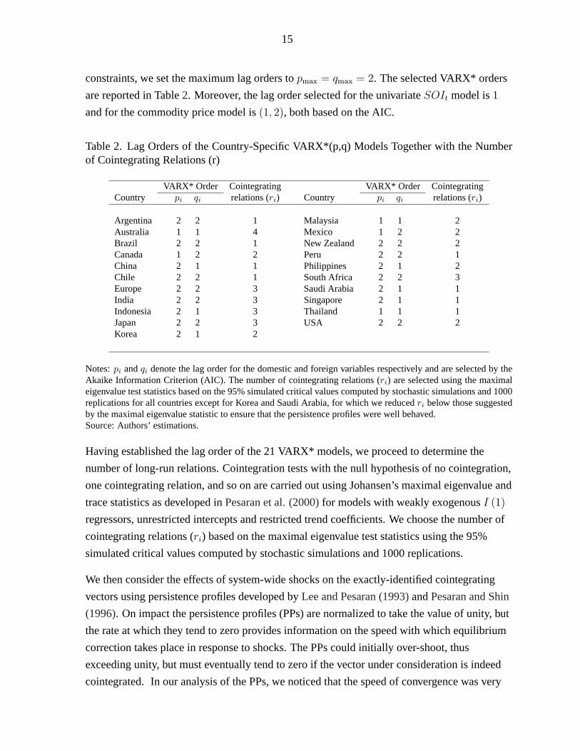
Table 2. Lag Orders of the Country-Specific VARX*(p,q) Models Together with the Number

of Cointegrating Relations (r)

VARX* Order Cointegrating VARX* Order Cointegrating

Country pi qi relations (ri) Country pi qi relations (ri)

Argentina 2 2 1 Malaysia 1 1 2

Australia 1 1 4 Mexico 1 2 2

Brazil 2 2 1 New Zealand 2 2 2

Canada 1 2 2 Peru 2 2 1

China 2 1 1 Philippines 2 1 2

Chile 2 2 1 South Africa 2 2 3

Europe 2 2 3 Saudi Arabia 2 1 1

India 2 2 3 Singapore 2 1 1

Indonesia 2 1 3 Thailand 1 1 1

Japan 2 2 3 USA 2 2 2

Korea 2 1 2

Notes: pi and qi denote the lag order for the domestic and foreign variables respectively and are selected by the

Akaike Information Criterion (AIC). The number of cointegrating relations (ri) are selected using the maximal

eigenvalue test statistics based on the 95% simulated critical values computed by stochastic simulations and 1000

replications for all countries except for Korea and Saudi Arabia, for which we reduced ri below those suggested

by the maximal eigenvalue statistic to ensure that the persistence profiles were well behaved.

Source: Authors’ estimations.

Having established the lag order of the 21 VARX* models, we proceed to determine the

number of long-run relations. Cointegration tests with the null hypothesis of no cointegration,

one cointegrating relation, and so on are carried out using Johansen’s maximal eigenvalue and

trace statistics as developed in Pesaran et al. (2000) for models with weakly exogenous I (1)

regressors, unrestricted intercepts and restricted trend coefficients. We choose the number of

cointegrating relations (ri) based on the maximal eigenvalue test statistics using the 95%

simulated critical values computed by stochastic simulations and 1000 replications.

We then consider the effects of system-wide shocks on the exactly-identified cointegrating

vectors using persistence profiles developed by Lee and Pesaran (1993) and Pesaran and Shin

(1996). On impact the persistence profiles (PPs) are normalized to take the value of unity, but

the rate at which they tend to zero provides information on the speed with which equilibrium

correction takes place in response to shocks. The PPs could initially over-shoot, thus

exceeding unity, but must eventually tend to zero if the vector under consideration is indeed

cointegrated. In our analysis of the PPs, we noticed that the speed of convergence was very

16

slow for Korea and for Saudi Arabia where the system-wide shocks never really died out, so

we reduced ri by one for each country resulting in well behaved PPs overall. The final

selection of the number of cointegrating relations are reported in Table 2.

A. The Effects of El Niño on Real Output

In general, identification of shocks in economics is not a straightforward task, however, in our

application it is clear that the El Niño shock, a negative unit shock (equal to one standard

error) to SOI anomalies, SOIt, is identified by construction (as ωt are "causal"). Table 3

reports the estimated median impulse responses of real GDP growth to an El Niño shock,

where the median responses on impact as well as the cumulated effects after the first, second,

third, and fourth quarters are reported. The results show that an El Niño event has a

statistically significant effect on real GDP growth for most of the countries in our

sample—there are only four countries for which the median effects are not statistically

significant at two or one standard deviations.10

As noted earlier, El Niño causes hot and dry summers in southeast Australia (Figure 3);

increases the frequency and severity of bush fires; reduces wheat export, and drives up global

wheat prices. Exports and global prices of other commodities (food and raw agricultural

materials) are also affected by drought in Australia, further reducing output growth (the

primary sector constitutes 10% of Australia’s GDP, Table 4). New Zealand often experiences

drought in parts of the country that are normally dry and floods in other places, resulting in

lower agricultural output (the El Niño of 1997/98 was particularly severe in terms of output

loss for New Zealand). Therefore, it is not surprising that we observe a statistically-significant

drop in GDP growth of 0.37% for Australia and 0.29% for New Zealand, three and one

quarters after an El Niño shock, respectively.11

Moreover, El Niño conditions usually coincide with a period of weak monsoon and rising

temperatures in India (see Figure 3) which adversely affects India’s agricultural sector and

increases domestic food prices. This is confirmed by our econometric analysis where India’s

GDP growth falls by 0.15% after the first quarter. The negative effect of El Niño is rather

muted in India, due to a number of mitigating factors. One such factor is the declining share

10Note that significance (for a particular variable and country) does not have to be seen on impact as the effects

of El Niño in most regions are felt during one specific season and hence could happen in a particular quarter rather

than all quarters.

11See Kamber et al. (2013) for an analysis of the economic effects of drought in New Zealand.

17

Table 3. The Effects of an El Niño Shock on Real GDP Growth (in percent)

Country Impact Cumulated Responses After

1 Quarter 2 Quarters 3 Quarters 4 Quarters

Argentina -0.08 0.03 0.29∗ 0.64∗∗ 1.08∗∗

Australia -0.03 -0.18∗∗ -0.30∗∗ -0.37∗ -0.41

Brazil -0.06 0.04 0.20 0.42∗ 0.68∗

Canada 0.00 0.13∗∗ 0.33∗ 0.58∗∗ 0.85∗∗

China -0.01 0.03 0.16∗ 0.36∗ 0.56∗

Chile -0.19∗ -0.10 0.16∗ 0.42∗ 0.70∗

Europe 0.02 0.09 0.27∗∗ 0.49∗∗ 0.69∗∗

India -0.03 -0.15∗ -0.23 -0.25 -0.25

Indonesia -0.35∗∗ -0.61∗ -0.91∗ -1.02 -1.01

Japan -0.10∗ -0.12 0.01∗ 0.20∗ 0.37∗

Korea 0.11 0.29∗ 0.44 0.58 0.67

Malaysia 0.08 0.06 0.13 0.27 0.43

Mexico 0.03 0.37∗∗ 0.71∗ 1.12∗ 1.57∗∗

New Zealand -0.16∗∗ -0.29∗ -0.37 -0.42 -0.43

Peru -0.07 -0.28 -0.35 -0.34 -0.33

Philippines 0.06 0.09 0.11 0.17 0.21

South Africa -0.11∗∗ -0.24∗ -0.47∗∗ -0.63∗ -0.72

Saudi Arabia -0.09 -0.17 -0.14 0.00 0.18

Singapore 0.09 0.28∗ 0.54∗ 0.87∗ 1.18∗

Thailand 0.47∗∗ 0.78∗∗ 1.11∗∗ 1.49∗∗ 1.81∗∗

USA 0.05∗ 0.10 0.23∗ 0.39∗ 0.55∗

Notes: Figures are median impulse responses to a one standard deviation reduction in SOI anomalies. The impact

is in percentage points and the horizon is quarterly. Symbols ** and * denote significance at 5–95% and 16–84%

bootstrapped error bounds respectively.

Source: Authors’ estimations.

Table 4. Share of Primary Sector in GDP (in percent), Averages over 2004-2013

Asia and Pacific North America

Australia 10 Canada 10

China 11 Mexico 12

India 21 United States 3

Indonesia 25

Japan 1 South America

Korea 3 Argentina 11

Malaysia 22 Brazil 7

New Zealand 6 Chile 18

Philippines 14 Peru 20

Singapore 0

Thailand 15 Africa

South Africa 10

Notes: Primary sector is the sum of agriculture, forestry, fishing and mining.

Source: Haver.

18

of agricultural output in Indian GDP over time—the share of India’s primary sector in GDP

was 28% in 1997 and has dropped to 20% in 2013. The increase in the contribution of Rabi

crops (sown in winter and harvested in the spring) and the decline in the contribution of

Kharif crops (sown in the rainy monsoon season) over the past few decades is another

mitigating factor as sowing of Rabi crops is not “directly” affected by the monsoon.12 Note

also that the total irrigated area for major crops in India has increased from 22.6 million

hectares in 1950-51 to 86.4 million hectares in 2009-10. Moreover, due to more developed

agricultural markets and policies, rising agriculture yield, and climatological early warning

systems, farmers are better able to switch to more drought-resistant and short-duration crops

(with government assistance), at reasonably short notice. Furthermore, any severe rainfall

deficiency in India could have implications for public agricultural spending and government

finances. However, one should note that an El Niño year has not always resulted in weak

monsoons in India, see Saini and Gulati (2014).

Drought in Indonesia is also harmful for the local economy, and pushes up world prices for

coffee, cocoa, and palm oil, among other commodities. Furthermore, mining equipment in

Indonesia relies heavily on hydropower; with deficient rain and low river currents, then less

nickel (which is used to strengthen steel) can be produced by the world’s top exporter of

nickel. Indonesian GDP growth falls by 0.91% at the end of the second quarter, and metal

prices increase as global supply drops. This large growth effect is expected given that the

share of the primary sector (agricultural and mining) in Indonesian GDP is around 25 percent

(see Table 4).

Looking beyond the Asia and Pacific region, South Africa also experiences hot and dry

summers during an El Niño episode (Figure 3), which has adverse effects on its agricultural

production (the primary sector makes up 10% of South Africa’s GDP) with the empirical

results suggesting a fall in GDP growth by 0.63% after the third quarter. Moreover, El Niño

typically brings stormy winters in Chile and affects metal prices through supply chain

disruption—heavy rain in Chile will reduce access to its mountainous mining regions, where

large copper deposits are found. Therefore, we would expect an increase in metal prices and a

reduction in output growth, which we estimate to be −0.19% on impact. More frequent

typhoon strikes and cooler weather during summers are expected for Japan, which could

depress consumer spending and growth. Our analysis suggests an initial drop of only 0.10%

in Japanese output growth. However, we also observe that for both Chile and Japan, the

12In 1980-81 the ratio of Kharif to Rabi crop production was 1.5. In 2013-14 it is estimated at 0.95 (see, India

Economic Survey 2014-15).

19

overall effect after four quarters is positive, by 0.70% and 0.37% respectively. This is most

likely due to positive spillovers from their major trading partners. For instance, trade with

China, Europe, and the U.S. constitutes over 57% of each country’s total trade (see Table 5).

The construction sector also sees a large boost following typhoons in Japan, which can partly

explain the increase in growth after an initial decline. Finally, for northern Brazil, there is a

high probability of a low rainfall year when El Niño is in force. Drought in northern parts of

Brazil can drive up world prices for coffee, sugar, and citrus. However, south-eastern Brazil

gets plentiful rain in the spring/summer of an El Niño year, which leads to higher agricultural

output. We do not observe any significant effects for Brazil in the first two quarters,

suggesting perhaps that the loss in agricultural output from drought in the northern part is to

some extent mitigated by above average yields in the south. More importantly, trade spillovers

from other Latin American countries and systemic countries (China, Europe, and the U.S.)

seem to suggest a positive overall effect on Brazil from an El Niño event in the third and

fourth quarters following the shock.

El Niño years feature below-normal rainfall for the Philippines. However, the authorities have

extensive early-warning systems in place, including conservation management of the water

supply for Manila. As a result, we do not observe any significant growth effects. Moreover,

the fisheries industry in Peru suffers because of the change in upwelling of nutrient-rich water

along the coast. As Peru is the world’s largest exporter of fishmeal used in animal feed, a

lower supply from Peru has ramifications for livestock prices worldwide. However, at the

same time agricultural output in Peru rises due to the wetter weather. Although the median

growth effect for Peru is negative (−0.33% after four quarters), it is in fact statistically

insignificant, so the positive growth effect from agricultural output (being 5.8% of GDP)

offsets the negative impact on the fisheries industry (constituting 0.6% of GDP).

While an El Niño event results in lower growth for some economies, others may actually

benefit due to lower temperatures, more rain, and less natural disasters. For instance, plentiful

rains can help boost soybeans production in Argentina, which exports 95% of the soybeans it

produces, and for which the primary sector is around 11% of GDP (Table 4). Canada enjoys

warmer weather in an El Niño year, and in particular a greater return from its fisheries. In

addition, the increase in oil prices means larger oil revenues for Canada, which is the world’s

fifth-largest oil producer (averaging 3,856 million barrels per day in 2012). For Mexico we

observe less hurricanes on the east coast and more hurricanes on the west coast, which brings

generally stability to the oil sector and boosts exports (oil revenue is around 8% of GDP in

Mexico). For the United States, El Niño typically brings wet weather to California (benefiting

crops such as limes, almonds and avocados), warmer winters in the Northeast, increased

20

Table 5. Trade Weights, Averages over 2009–2011

Arge

ntin

a

Aust

ralia

Braz

il

Cana

da

Chin

a

Chile

Euro

pe

Indi

a

Indo

nesia

Japa

n

Kore

a

Mal

aysia

Mex

ico

New

 Zea

land

Peru

Philip

pine

s

Sout

h Af

rica

Saud

i Ara

bia

Sing

apor

e

Thai

land

USA

Argentina 0.00 0.00 0.11 0.00 0.01 0.05 0.01 0.00 0.01 0.00 0.00 0.00 0.00 0.00 0.03 0.00 0.01 0.00 0.00 0.00 0.00Australia 0.01 0.00 0.01 0.00 0.04 0.01 0.03 0.04 0.03 0.06 0.04 0.04 0.00 0.24 0.00 0.02 0.02 0.01 0.03 0.05 0.01Brazil 0.32 0.01 0.00 0.01 0.03 0.08 0.04 0.02 0.01 0.01 0.02 0.01 0.01 0.00 0.06 0.00 0.02 0.02 0.01 0.01 0.02Canada 0.02 0.01 0.02 0.00 0.02 0.02 0.04 0.01 0.01 0.02 0.01 0.01 0.03 0.02 0.07 0.01 0.01 0.01 0.01 0.01 0.20China 0.13 0.25 0.19 0.08 0.00 0.24 0.25 0.16 0.14 0.27 0.28 0.16 0.09 0.16 0.19 0.12 0.18 0.15 0.14 0.16 0.18Chile 0.06 0.00 0.03 0.00 0.01 0.00 0.01 0.01 0.00 0.01 0.01 0.00 0.01 0.00 0.06 0.00 0.00 0.00 0.00 0.00 0.01Europe 0.21 0.15 0.28 0.12 0.23 0.19 0.00 0.30 0.11 0.14 0.12 0.13 0.08 0.16 0.20 0.13 0.38 0.19 0.14 0.15 0.22India 0.02 0.04 0.03 0.01 0.03 0.02 0.05 0.00 0.05 0.01 0.03 0.03 0.01 0.02 0.01 0.01 0.06 0.08 0.04 0.02 0.02Indonesia 0.01 0.03 0.01 0.00 0.02 0.00 0.01 0.04 0.00 0.04 0.04 0.05 0.00 0.02 0.00 0.03 0.01 0.02 0.10 0.05 0.01Japan 0.02 0.16 0.05 0.03 0.15 0.09 0.08 0.04 0.16 0.00 0.14 0.14 0.03 0.09 0.05 0.17 0.08 0.14 0.08 0.20 0.07Korea 0.02 0.07 0.04 0.01 0.10 0.06 0.04 0.04 0.08 0.08 0.00 0.05 0.03 0.04 0.04 0.07 0.03 0.11 0.07 0.04 0.03Malaysia 0.01 0.03 0.01 0.00 0.04 0.00 0.02 0.03 0.07 0.04 0.02 0.00 0.01 0.03 0.00 0.04 0.01 0.01 0.15 0.07 0.01Mexico 0.03 0.01 0.03 0.04 0.01 0.03 0.02 0.01 0.00 0.01 0.02 0.01 0.00 0.01 0.03 0.00 0.00 0.00 0.01 0.00 0.15New Zealand 0.00 0.04 0.00 0.00 0.00 0.00 0.00 0.00 0.00 0.00 0.00 0.00 0.00 0.00 0.00 0.01 0.00 0.00 0.00 0.00 0.00Peru 0.01 0.00 0.01 0.01 0.00 0.03 0.01 0.00 0.00 0.00 0.00 0.00 0.00 0.00 0.00 0.00 0.00 0.00 0.00 0.00 0.00Philippines 0.01 0.00 0.00 0.00 0.01 0.00 0.01 0.00 0.01 0.02 0.01 0.02 0.00 0.01 0.00 0.00 0.00 0.01 0.03 0.02 0.01South Africa 0.01 0.01 0.01 0.00 0.01 0.00 0.03 0.03 0.01 0.01 0.01 0.01 0.00 0.00 0.00 0.00 0.00 0.02 0.00 0.01 0.01Saudi Arabia 0.00 0.01 0.02 0.00 0.02 0.00 0.03 0.07 0.02 0.04 0.05 0.01 0.00 0.02 0.00 0.03 0.04 0.00 0.03 0.03 0.02Singapore 0.00 0.05 0.01 0.00 0.03 0.00 0.03 0.05 0.14 0.03 0.04 0.15 0.00 0.04 0.00 0.12 0.01 0.04 0.00 0.06 0.02Thailand 0.01 0.04 0.01 0.00 0.03 0.01 0.02 0.02 0.05 0.05 0.02 0.07 0.01 0.03 0.01 0.06 0.02 0.03 0.05 0.00 0.01USA 0.10 0.09 0.16 0.67 0.19 0.17 0.27 0.13 0.09 0.17 0.13 0.12 0.68 0.12 0.23 0.16 0.11 0.16 0.11 0.11 0.00

Notes: Trade weights are computed as shares of exports and imports, displayed in columns by country (such that

a column, but not a row, sum to 1).

Source: International Monetary Fund’s Direction of Trade Statistics, 2009-2011.

21

rainfall in the South, diminished tornadic activity in the Midwest, and a decrease in the

number of hurricanes that hit the East coast (see Figure 3). Therefore, not surprisingly, Table

3 shows an increase in GDP growth of 1.08%, 0.85%, 1.57%, and 0.55% in the fourth quarter

following an El Niño shock for Argentina, Canada, Mexico, and the U.S., respectively. These

estimates also take into account the positive spillover effects that an increase in U.S. GDP

growth has on the Canadian and Mexican economies, given the extensive trade exposure of

these two economies to the United States (trade weights are 67 and 68 percent respectively,

see Table 5) as well as other third-market effects. The positive growth effect of 0.55% for the

U.S. might seem large at first glance, however, it is not far from the estimated net benefits of

$15 billion following the severe El Niño event of 1997-1998, which is equivalent to 0.2% of

GDP, see Changnon (1999). These net benefits are calculated based on a direct cost-benefit

analysis—$4 billion (cost) and $19 billion (benefit)—and a larger shock associated with the

1997-98 El Niño event, but they do not take into account the indirect growth effects through

third markets, which is captured in our GVAR framework.

Although El Niño is associated with dry weather in northern China and wet weather in

southern China (Figure 3), it is not clear that we should observe any direct positive or negative

effects on China’s output growth. In fact Table 3 shows that initially there are no

statistically-significant effects following an El Niño shock, but Chinese GDP growth increases

by 0.56% in the fourth quarter following an El Niño shock. This is mainly due to positive

spillovers from trade with other major economies—Chinese trade with the U.S. is about 19%

of the total, and given that the U.S. is benefiting from an El Niño event, so does China.

Moreover, a number of economies which are not directly affected by El Niño do benefit from

the shock, mainly due to positive indirect spillovers from commercial trade and financial

market links. For instance, Europe experiences an increase in real GDP growth of 0.69% in

the fourth quarter following an El Niño event, and Singapore by 1.18% (mainly due to an

increase in the shipping industry following the increase in demand from U.S. and other major

economies).

B. The Effects of El Niño on Real Commodity Prices

The higher temperatures and droughts following an El Niño event, particularly in Asia-Pacific

countries, not only increases the prices of non-fuel commodities (by 5.31% after four quarters,

see Table 6), but also leads to higher demand for coal and crude oil as lower electricity output

is generated from both thermal power plants and hydroelectric dams. In addition, farmers

increase their water demand for irrigation purposes, which further increases the fuel demand

22

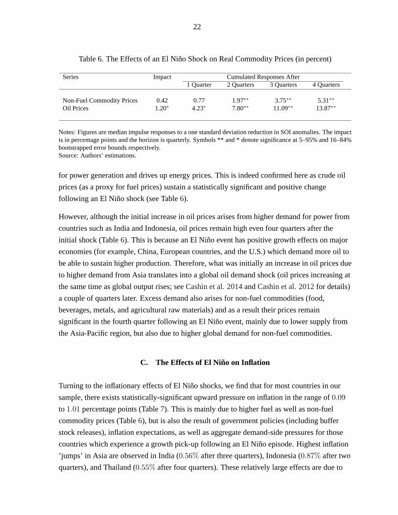
Table 6. The Effects of an El Niño Shock on Real Commodity Prices (in percent)

Series Impact Cumulated Responses After

1 Quarter 2 Quarters 3 Quarters 4 Quarters

Non-Fuel Commodity Prices 0.42 0.77 1.97∗∗ 3.75∗∗ 5.31∗∗

Oil Prices 1.20∗ 4.23∗ 7.80∗∗ 11.09∗∗ 13.87∗∗

Notes: Figures are median impulse responses to a one standard deviation reduction in SOI anomalies. The impact

is in percentage points and the horizon is quarterly. Symbols ** and * denote significance at 5–95% and 16–84%

bootstrapped error bounds respectively.

Source: Authors’ estimations.

for power generation and drives up energy prices. This is indeed confirmed here as crude oil

prices (as a proxy for fuel prices) sustain a statistically significant and positive change

following an El Niño shock (see Table 6).

However, although the initial increase in oil prices arises from higher demand for power from

countries such as India and Indonesia, oil prices remain high even four quarters after the

initial shock (Table 6). This is because an El Niño event has positive growth effects on major

economies (for example, China, European countries, and the U.S.) which demand more oil to

be able to sustain higher production. Therefore, what was initially an increase in oil prices due

to higher demand from Asia translates into a global oil demand shock (oil prices increasing at

the same time as global output rises; see Cashin et al. 2014 and Cashin et al. 2012 for details)

a couple of quarters later. Excess demand also arises for non-fuel commodities (food,

beverages, metals, and agricultural raw materials) and as a result their prices remain

significant in the fourth quarter following an El Niño event, mainly due to lower supply from

the Asia-Pacific region, but also due to higher global demand for non-fuel commodities.

C. The Effects of El Niño on Inflation

Turning to the inflationary effects of El Niño shocks, we find that for most countries in our

sample, there exists statistically-significant upward pressure on inflation in the range of 0.09

to 1.01 percentage points (Table 7). This is mainly due to higher fuel as well as non-fuel

commodity prices (Table 6), but is also the result of government policies (including buffer

stock releases), inflation expectations, as well as aggregate demand-side pressures for those

countries which experience a growth pick-up following an El Niño episode. Highest inflation

’jumps’ in Asia are observed in India (0.56% after three quarters), Indonesia (0.87% after two

quarters), and Thailand (0.55% after four quarters). These relatively large effects are due to

23

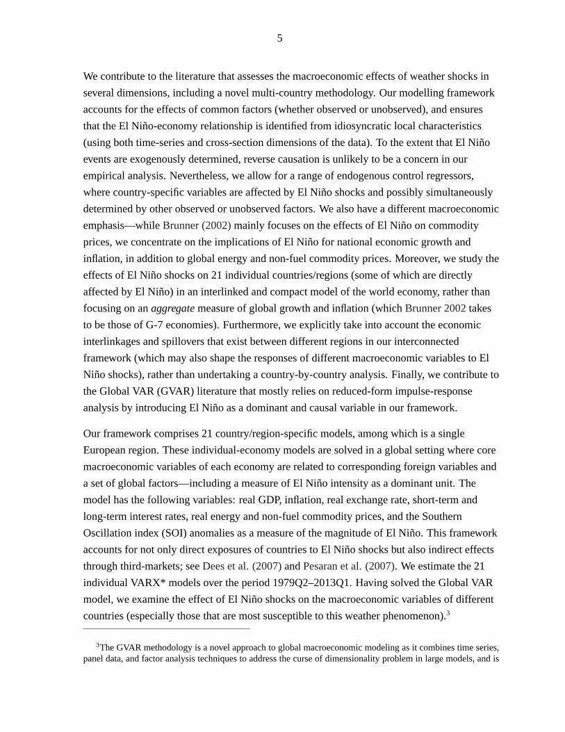
the high weight placed on food in the CPI basket of these countries: 47.6%, 32.7% and 33.5%,

respectively. To examine this further we plot the weight of food in the CPI basket of the 20

countries in our sample and the European region against the median impulse responses of

inflation to an El Niño shock in those countries. Figure 5 shows a clear positive relationship

between the two variables, with a correlation of 0.5, thereby providing further support to the

null hypothesis that inflation responses are larger in economies that have higher share of food

in their CPI baskets.

Note that production of perishables (i.e. fruits and vegetables) in India is affected less by

monsoon than food grains, while the prices of fruits and vegetables are relatively more

volatile. Moreover, inflation in food grains has historically been affected by government

procurement policies and administered minimum support prices in agriculture. During the last

decade, inflation increased sharply after the 2009 drought in India, however, in the previous

episodes of drought in 2002 and 2004, inflation remained subdued. In 2009, drought

conditions were accompanied by a steep increase in minimum support prices, resulting in high

food grain inflation and consequently higher CPI inflation.13 Overall, government policies,

tight monetary stances, high water reservoir levels, and excess food grain stocks could partly

offset the inflationary impact of El Niño shocks on prices in India. For other Asian

economies, which generally place lower weight on food in the CPI index, we notice a smaller

increase in inflation: China by 0.11% (32.5), Japan by 0.10% (24), Korea by 0.44% (13.9),

Malaysia by 0.28% (30.3), and Philippines by 0.19% (39), with the numbers in brackets

representing the weight of food as a percentage of total consumption in the CPI basket.

Inflation in the U.S. and Europe increases by smaller amounts 0.14 and 0.09 percentage

points, respectively, but perhaps surprisingly Mexico sees an increase of 1.01% after two

quarters (with a 21 percent food share in its CPI basket). Finally, in South America inflation

in the fourth quarter following an El Niño event increases by between 0.39% and 0.97%, but it

is only statistically significant for Chile with an increase of 0.39%. There are only two

countries that experience a reduction in inflation following an El Niño event—New Zealand

by 0.61% after four quarters and Singapore by 0.07% on impact. For the former, this can be

explained by very large disinflation pressures during the initial occurrences of the El Niño

(recessions, wage and price freezes, and structural reforms), and its well-anchored inflation

expectations14—with an inflation target range of 1–3% on average over the medium-term and

13During the years 2002, 2004 and 2009 (all years of poor monsoons), CPI inflation averaged 4.1%, 3.9%, and

12.3% in India, respectively.

14See also Buckle et al. (2002) for similar findings.

24

Table 7. The Effects of an El Niño Shock on Inflation (in percent)

Country Impact Cumulated Responses After

1 Quarter 2 Quarters 3 Quarters 4 Quarters

Argentina 0.51 0.79 0.57 0.92 0.64

Australia -0.01 0.02 0.02 0.01 0.00

Brazil -0.30 -0.21 1.01 1.49 0.97

Canada -0.05∗ -0.10 -0.08 -0.07 -0.07

China 0.00 -0.02 0.00 0.06∗ 0.11∗

Chile 0.14∗∗ 0.14 0.29∗∗ 0.32 0.39∗

Europe 0.00 0.00 0.02 0.06∗ 0.09∗

India 0.15∗ 0.16 0.42∗∗ 0.56∗∗ 0.60

Indonesia 0.25∗ 0.61∗∗ 0.87∗ 0.95 0.91

Japan 0.03∗ 0.05 0.04 0.06 0.10∗∗

Korea 0.01 0.12∗∗ 0.22∗∗ 0.34∗∗ 0.44∗∗

Malaysia 0.05∗ 0.09 0.16∗ 0.23∗ 0.28∗

Mexico 0.22 0.60∗ 1.01∗ 1.12 1.04

New Zealand -0.06 -0.23∗∗ -0.39∗∗ -0.55∗∗ -0.61∗

Peru -0.06 -0.73 -0.48 -0.38 0.65

Philippines 0.11 0.06 0.19∗ 0.22 0.27

South Africa 0.10∗∗ -0.01∗∗ 0.02 0.06 0.09

Saudi Arabia 0.01 -0.03∗ -0.02 -0.01 -0.02

Singapore -0.07∗∗ -0.06 -0.06 -0.06 -0.06

Thailand 0.01 0.21∗∗ 0.35∗∗ 0.46∗∗ 0.55∗∗

USA 0.01 0.02 0.10∗ 0.14∗ 0.15

Notes: Figures are median impulse responses to a one standard deviation reduction in SOI anomalies. The impact

is in percentage points and the horizon is quarterly. Symbols ** and * denote significance at 5–95% and 16–84%

bootstrapped error bounds respectively.

Source: Authors’ estimations.

Figure 5. Food Weight in CPI Basket and Inflation Responses

Source: Authors’ calculations based on data from Haver and impulse response estimates in Table 7.

25

an average CPI inflation of around 2.5% since 1990.

D. Robustness Checks

To make sure that our results are not driven by the type of weights used to create

country-specific foreign variable or solve the GVAR model as a whole, we experimented

using Trade in Value Added (TiVA) weights (to account for supply chain factors) and found

the impulse responses to be very similar to those with trade weights, wij , as used above.

Therefore, as is now standard in the literature, we only report the results with the weights

calculated as the average of exports and imports of country i with j (Table 5). We also

estimated our model with the foreign variables computed using trade weights averaged over

2007-2009 and 2000-2013, and obtained very similar results to the benchmark weights

(2009-2011) used in the earlier analysis. Moreover, we estimated a version of the model

splitting the European region into Euro Area and 5 separate country VARX* models, thereby

having a total of 26 country/region-specific VARX* models, and found the results to be robust

to these changes. These results are not reported here, but are available on request.

V. CONCLUDING REMARKS

This paper contributed to the climate-macroeconomy literature by exploiting exogenous

variation in El Niño weather events over time to causatively identify the effects of El Niño

shocks on growth, inflation, energy and non-fuel commodity prices. To analyze the

international macroeconomic transmission of El Niño shocks we estimated a Global VAR

(GVAR) model for 21 countries/regions over the period 1979Q2–2013Q1. Our modelling

framework took into account real and financial drivers of economic activity; interlinkages and

spillovers that exist between different regions; and the effects of unobserved or observed

common factors (e.g. energy and non-fuel commodity prices). This is crucial as the impact of

El Niño shocks cannot be reduced to one country, but rather involves multiple regions, and

may be amplified or reduced depending on the degree of openness of the countries and their

trade structure.

We showed that there are considerable heterogeneities in the responses of different countries

to El Niño shocks. While Australia, Chile, Indonesia, India, Japan, New Zealand and South

Africa face a short-lived fall in economic activity following an El Niño weather shock, the

United States, Europe and China actually benefit (possibly indirectly through third-market

26

effects) from such a climatological change. We also found that most countries in our sample

experience short-run inflationary pressures following an El Niño episode, as global energy

and non-fuel commodity prices increase.

The sensitivity of growth and inflation in different countries, as well as global commodity

prices, to El Niño developments raises the question of which policies and institutions are

needed to counter the adverse effects of such shocks. These measures could include changes

in the cropping pattern and input use (e.g. seeds of quicker-maturing crop varieties), rainwater

conservation, judicious release of food grain stocks, and changes in imports

policies/quantities—these measures would all help to bolster agricultural production in

low-rainfall El Niño years. On the macroeconomic policy side, any uptick in inflation arising

from El Niño shocks could be accompanied by a tightening of the monetary stance (if

second-round effects emerge), to help anchor inflation expectations. Investment in agriculture

sector, mainly in irrigation, as well as building more efficient food value chains should also be

considered in the longer-term. Our results also have policy implications for the design of

appropriate bands around inflation targets in countries that are directly affected by El Niño

shocks. This depends on the share of food in their CPI basket and structural-food inflation, as

well as their susceptibility to El Niño shocks.

The research in this paper can be extended in a number of directions. A more complete model

for the climate, including perhaps temperature, precipitation, storms, and other aspects of the

weather, could be developed and integrated within our compact model of the world economy.

This framework could then be utilized to investigate the effects of climate change and/or

global weather shocks on economic activity. Modelling the global climate, however, is in

itself a major task and we shall therefore leave it as a task for future research.

27

REFERENCES

Adams, R. M., K. J. Bryant, B. A. Mccarl, D. M. Legler, J. O’Brien, A. Solow, and

R. Weiher (1995). Value of Improved Long-Range Weather Information. Contemporary

Economic Policy 13(3), 10–19.

Baxter, M. and M. A. Kouparitsas (2005). Determinants of Business Cycle Comovement: A

Robust Analysis. Journal of Monetary Economics 52(1), pp. 113–157.

Bennetton, J., P. Cashin, D. Jones, and J. Soligo (1998). An Economic Evaluation of

Bushfire Prevention and Suppression. Australian Journal of Agricultural and Resource

Economics 42(2), 149–175.

Brunner, A. D. (2002). El Nino and World Primary Commodity Prices: Warm Water or Hot

Air? Review of Economics and Statistics 84(1), 176–183.

Buckle, R. A., K. Kim, H. Kirkham, N. McLellan, and J. Sharma (2002). A Structural VAR

Model of the New Zealand Business Cycle. New Zealand Treasury Working Paper

02/26.

Cashin, P., K. Mohaddes, and M. Raissi (2012). The Global Impact of the Systemic

Economies and MENA Business Cycles. IMF Working Paper WP/12/255.

Cashin, P., K. Mohaddes, M. Raissi, and M. Raissi (2014). The Differential Effects of Oil

Demand and Supply Shocks on the Global Economy. Energy Economics 44, 113–134.

Changnon, S. A. (1999). Impacts of 1997-98 El Niño Generated Weather in the United

States. Bulletin of the American Meteorological Society 80, 1819–1827.

Chudik, A. and M. H. Pesaran (2013). Econometric Analysis of High Dimensional VARs

Featuring a Dominant Unit. Econometric Reviews 32(5-6), 592–649.

Chudik, A. and M. H. Pesaran (2014). Theory and Practice of GVAR Modeling. Journal of

Economic Surveys, forthcoming.

Debelle, G. and G. Stevens (1995). Monetary Policy Goals for Inflation in Australia. Reserve

Bank of Australia Research Discussion Paper 9503.

Dees, S., F. di Mauro, M. H. Pesaran, and L. V. Smith (2007). Exploring the International

28

Linkages of the Euro Area: A Global VAR Analysis. Journal of Applied

Econometrics 22, 1–38.

Dell, M., B. F. Jones, and B. A. Olken (2014). What Do We Learn from the Weather? The

New Climate-Economy Literature. Journal of Economic Literature 52(3), 740–98.

Handler, P. and E. Handler (1983). Climatic Anomalies in the Tropical Pacific Ocean and

Corn Yields in the United States. Science 220(4602), 1155–1156.

Hsiang, S. M., K. C. Meng, and M. A. Cane (2011). Civil Conflicts are Associated with the

Global Climate. Nature 476, 438–441.

Iizumi, T., J.-J. Luo, A. J. Challinor, G. Sakurai, M. Yokozawa, H. Sakuma, M. E. Brown,

and T. Yamagata (2014). Impacts of El Niño Southern Oscillation on the Global Yields

of Major Crops. Nature Communications 5.

Kamber, G., C. McDonald, and G. Price (2013). Drying Out: Investigating the Economic

Effects of Drought in New Zealand. Reserve Bank of New Zealand Analytical Note

Series AN2013/02.

Lee, K. and M. H. Pesaran (1993). Persistence Profiles and Business Cycle Fluctuations in a

Disaggregated Model of UK Output Growth. Ricerche Economiche 47, 293–322.

Mohaddes, K. and M. H. Pesaran (2015). Oil Supply Shocks and the Global Economy: A

Counterfactual Analysis. Cambridge Working Papers in Economics, forthcoming.

Pesaran, M. H. (2004). General Diagnostic Tests for Cross Section Dependence in Panels.

IZA Discussion Paper No. 1240.

Pesaran, M. H. and Y. Shin (1996). Cointegration and Speed of Convergence to Equilibrium.

Journal of Econometrics 71, 117–143.

Pesaran, M. H., Y. Shin, and R. J. Smith (2000). Structural Analysis of Vector Error

Correction Models with Exogenous I(1) Variables. Journal of Econometrics 97,

293–343.

Pesaran, M. H., L. Vanessa Smith, and R. P. Smith (2007). What if the UK or Sweden had

Joined the Euro in 1999? An Empirical Evaluation Using a Global VAR. International

Journal of Finance & Economics 12(1), 55–87.

29

Pidwirny, M. (2006). El Niño, La Niña and the Southern Oscillation. In Fundamentals of

Physical Geography, 2nd Edition.

Saini, S. and A. Gulati (2014). El Niño and Indian Droughts - A Scoping Exercise. Indian

Council for Research on International Economic Relations Working Paper 276.

Smith, L. V. and A. Galesi (2014). GVAR Toolbox 2.0. University of Cambridge: Judge

Business School.

Solow, A., R. Adams, K. Bryant, D. Legler, J. O’Brien, B. McCarl, W. Nayda, and R. Weiher

(1998). The Value of Improved ENSO Prediction to U.S. Agriculture. Climatic

Change 39(1), 47–60.

Tol, R. S. J. (2009). The Economic Effects of Climate Change. Journal of Economic

Perspectives 23(2), 29–51.

Ubilava, D. (2012). El Niño, La Niña, and World Coffee Price Dynamics. Agricultural

Economics 43(1), 17–26.