Fair Value Measurement Illustrative Examples - …€¦ · advanced stage of development that would compete with the project if completed and the project would be expected to improve

Fair Value Measurement Illustrative Examples

SB-FRS 113 STATUTORY BOARD FINANCIAL

REPORTING STANDARD

SB-FRS 113 IE

2

CONTENTS

from paragraph

HIGHEST AND BEST USE AND VALUATION PREMISE Example 1—Asset group Example 2—Land Example 3—Research and development project USE OF MULTIPLE VALUATION TECHNIQUES Example 4—Machine held and used Example 5—Software asset PRINCIPAL (OR MOST ADVANTAGEOUS) MARKET Example 6—Level 1 principal (or most advantageous) market TRANSACTION PRICES AND FAIR VALUE AT INITIAL RECOGNITION Example 7—Interest rate swap at initial recognition RESTRICTED ASSETS Example 8—Restriction on the sale of an equity instrument Example 9—Restrictions on the use of an asset MEASURING LIABILITIES Example 10—Structured note Example 11—Decommissioning liability Example 12—Debt obligation: quoted price Example 13—Debt obligation: present value technique MEASURING FAIR VALUE WHEN THE VOLUME OR LEVEL OF ACTIVITY FOR AN ASSET OR A LIABILITY HAS SIGNIFICANTLY DECREASED Example 14—Estimating a market rate of return when the volume or level of activity for an asset has significantly decreased FAIR VALUE DISCLOSURES Example 15—Assets measured at fair value Example 16—Reconciliation of fair value measurements categorised within Level 3 of the fair value hierarchy Example 17—Valuation techniques and inputs Example 18—Valuation processes

IE2

IE3

IE7

IE9

IE10

IE11

IE15

IE18

IE19

IE23

IE24

IE27

IE28

IE29

IE30

IE34

IE35

IE40

IE43

IE48

IE49

IE59

IE60

IE61

IE63

IE65

SB-FRS 113 IE

3

Example 19—Information about sensitivity to changes in significant unobservable inputs APPENDIX Amendments to guidance on other SB-FRSs

IE66

SB-FRS 113 IE

4

Illustrative Examples These examples accompany, but are not part of, SB-FRS 113. They illustrate aspects of SB-FRS 113 but are not intended to provide interpretative guidance. IE1 These examples portray hypothetical situations illustrating the judgements that might apply

when an entity measures assets and liabilities at fair value in different valuation situations. Although some aspects of the examples may be present in actual fact patterns, all relevant facts and circumstances of a particular fact pattern would need to be evaluated when applying SB-FRS 113.

Highest and best use and valuation premise IE2 Examples 1–3 illustrate the application of the highest and best use and valuation premise

concepts for non-financial assets.

Example 1—Asset group IE3 An entity acquires assets and assumes liabilities in a business combination. One of the groups

of assets acquired comprises Assets A, B and C. Asset C is billing software integral to the business developed by the acquired entity for its own use in conjunction with Assets A and B (ie the related assets). The entity measures the fair value of each of the assets individually, consistently with the specified unit of account for the assets. The entity determines that the highest and best use of the assets is their current use and that each asset would provide maximum value to market participants principally through its use in combination with other assets or with other assets and liabilities (ie its complementary assets and the associated liabilities). There is no evidence to suggest that the current use of the assets is not their highest and best use.

IE4 In this situation, the entity would sell the assets in the market in which it initially acquired the

assets (ie the entry and exit markets from the perspective of the entity are the same). Market participant buyers with whom the entity would enter into a transaction in that market have characteristics that are generally representative of both strategic buyers (such as competitors) and financial buyers (such as private equity or venture capital firms that do not have complementary investments) and include those buyers that initially bid for the assets. Although market participant buyers might be broadly classified as strategic or financial buyers, in many cases there will be differences among the market participant buyers within each of those groups, reflecting, for example, different uses for an asset and different operating strategies.

IE5 As discussed below, differences between the indicated fair values of the individual assets relate

principally to the use of the assets by those market participants within different asset groups:

(a) Strategic buyer asset group. The entity determines that strategic buyers have related assets that would enhance the value of the group within which the assets would be used (ie market participant synergies). Those assets include a substitute asset for Asset C (the billing software), which would be used for only a limited transition period and could not be sold on its own at the end of that period. Because strategic buyers have substitute assets, Asset C would not be used for its full remaining economic life. The indicated fair values of Assets A, B and C within the strategic buyer asset group (reflecting the synergies resulting from the use of the assets within that group) are CU360,1 CU260 and CU30, respectively. The indicated fair value of the assets as a group within the strategic buyer asset group is CU650.

(b) Financial buyer asset group. The entity determines that financial buyers do not have

related or substitute assets that would enhance the value of the group within which the assets would be used. Because financial buyers do not have substitute assets, Asset

1 In these examples, monetary amounts are denominated in ‘currency units (CU)’.

SB-FRS 113 IE

5

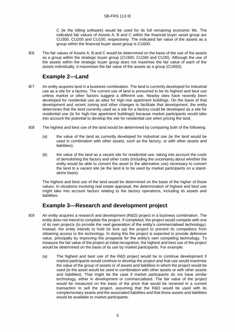
C (ie the billing software) would be used for its full remaining economic life. The indicated fair values of Assets A, B and C within the financial buyer asset group are CU300, CU200 and CU100, respectively. The indicated fair value of the assets as a group within the financial buyer asset group is CU600.

IE6 The fair values of Assets A, B and C would be determined on the basis of the use of the assets

as a group within the strategic buyer group (CU360, CU260 and CU30). Although the use of the assets within the strategic buyer group does not maximise the fair value of each of the assets individually, it maximises the fair value of the assets as a group (CU650).

Example 2—Land IE7 An entity acquires land in a business combination. The land is currently developed for industrial

use as a site for a factory. The current use of land is presumed to be its highest and best use unless market or other factors suggest a different use. Nearby sites have recently been developed for residential use as sites for high-rise apartment buildings. On the basis of that development and recent zoning and other changes to facilitate that development, the entity determines that the land currently used as a site for a factory could be developed as a site for residential use (ie for high-rise apartment buildings) because market participants would take into account the potential to develop the site for residential use when pricing the land.

IE8 The highest and best use of the land would be determined by comparing both of the following:

(a) the value of the land as currently developed for industrial use (ie the land would be used in combination with other assets, such as the factory, or with other assets and liabilities).

(b) the value of the land as a vacant site for residential use, taking into account the costs

of demolishing the factory and other costs (including the uncertainty about whether the entity would be able to convert the asset to the alternative use) necessary to convert the land to a vacant site (ie the land is to be used by market participants on a stand-alone basis).

The highest and best use of the land would be determined on the basis of the higher of those values. In situations involving real estate appraisal, the determination of highest and best use might take into account factors relating to the factory operations, including its assets and liabilities.

Example 3—Research and development project IE9 An entity acquires a research and development (R&D) project in a business combination. The

entity does not intend to complete the project. If completed, the project would compete with one of its own projects (to provide the next generation of the entity’s commercialised technology). Instead, the entity intends to hold (ie lock up) the project to prevent its competitors from obtaining access to the technology. In doing this the project is expected to provide defensive value, principally by improving the prospects for the entity’s own competing technology. To measure the fair value of the project at initial recognition, the highest and best use of the project would be determined on the basis of its use by market participants. For example:

(a) The highest and best use of the R&D project would be to continue development if

market participants would continue to develop the project and that use would maximise the value of the group of assets or of assets and liabilities in which the project would be used (ie the asset would be used in combination with other assets or with other assets and liabilities). That might be the case if market participants do not have similar technology, either in development or commercialised. The fair value of the project would be measured on the basis of the price that would be received in a current transaction to sell the project, assuming that the R&D would be used with its complementary assets and the associated liabilities and that those assets and liabilities would be available to market participants.

SB-FRS 113 IE

6

(b) The highest and best use of the R&D project would be to cease development if, for

competitive reasons, market participants would lock up the project and that use would maximise the value of the group of assets or of assets and liabilities in which the project would be used. That might be the case if market participants have technology in a more advanced stage of development that would compete with the project if completed and the project would be expected to improve the prospects for their own competing technology if locked up. The fair value of the project would be measured on the basis of the price that would be received in a current transaction to sell the project, assuming that the R&D would be used (ie locked up) with its complementary assets and the associated liabilities and that those assets and liabilities would be available to market participants.

(c) The highest and best use of the R&D project would be to cease development if market

participants would discontinue its development. That might be the case if the project is not expected to provide a market rate of return if completed and would not otherwise provide defensive value if locked up. The fair value of the project would be measured on the basis of the price that would be received in a current transaction to sell the project on its own (which might be zero).

Use of multiple valuation techniques IE10 The SB-FRS notes that a single valuation technique will be appropriate in some cases. In other

cases multiple valuation techniques will be appropriate. Examples 4 and 5 illustrate the use of multiple valuation techniques.

Example 4—Machine held and used IE11 An entity acquires a machine in a business combination. The machine will be held and used in

its operations. The machine was originally purchased by the acquired entity from an outside vendor and, before the business combination, was customised by the acquired entity for use in its operations. However, the customisation of the machine was not extensive. The acquiring entity determines that the asset would provide maximum value to market participants through its use in combination with other assets or with other assets and liabilities (as installed or otherwise configured for use). There is no evidence to suggest that the current use of the machine is not its highest and best use. Therefore, the highest and best use of the machine is its current use in combination with other assets or with other assets and liabilities.

IE12 The entity determines that sufficient data are available to apply the cost approach and,

because the customisation of the machine was not extensive, the market approach. The income approach is not used because the machine does not have a separately identifiable income stream from which to develop reliable estimates of future cash flows. Furthermore, information about short-term and intermediate-term lease rates for similar used machinery that otherwise could be used to project an income stream (ie lease payments over remaining service lives) is not available. The market and cost approaches are applied as follows:

(a) The market approach is applied using quoted prices for similar machines adjusted for

differences between the machine (as customised) and the similar machines. The measurement reflects the price that would be received for the machine in its current condition (used) and location (installed and configured for use). The fair value indicated by that approach ranges from CU40,000 to CU48,000.

SB-FRS 113 IE

7

(b) The cost approach is applied by estimating the amount that would be required currently to construct a substitute (customised) machine of comparable utility. The estimate takes into account the condition of the machine and the environment in which it operates, including physical wear and tear (ie physical deterioration), improvements in technology (ie functional obsolescence), conditions external to the condition of the machine such as a decline in the market demand for similar machines (ie economic obsolescence) and installation costs. The fair value indicated by that approach ranges from CU40,000 to CU52,000.

IE13 The entity determines that the higher end of the range indicated by the market approach is most

representative of fair value and, therefore, ascribes more weight to the results of the market approach. That determination is made on the basis of the relative subjectivity of the inputs, taking into account the degree of comparability between the machine and the similar machines. In particular: (a) the inputs used in the market approach (quoted prices for similar machines) require

fewer and less subjective adjustments than the inputs used in the cost approach. (b) the range indicated by the market approach overlaps with, but is narrower than, the

range indicated by the cost approach. (c) there are no known unexplained differences (between the machine and the similar

machines) within that range.

Accordingly, the entity determines that the fair value of the machine is CU48,000.

IE14 If customisation of the machine was extensive or if there were not sufficient data available to apply the market approach (eg because market data reflect transactions for machines used on a stand-alone basis, such as a scrap value for specialised assets, rather than machines used in combination with other assets or with other assets and liabilities), the entity would apply the cost approach. When an asset is used in combination with other assets or with other assets and liabilities, the cost approach assumes the sale of the machine to a market participant buyer with the complementary assets and the associated liabilities. The price received for the sale of the machine (ie an exit price) would not be more than either of the following:

(a) the cost that a market participant buyer would incur to acquire or construct a substitute

machine of comparable utility; or (b) the economic benefit that a market participant buyer would derive from the use of the

machine.

Example 5—Software asset IE15 An entity acquires a group of assets. The asset group includes an income-producing software

asset internally developed for licensing to customers and its complementary assets (including a related database with which the software asset is used) and the associated liabilities. To allocate the cost of the group to the individual assets acquired, the entity measures the fair value of the software asset. The entity determines that the software asset would provide maximum value to market participants through its use in combination with other assets or with other assets and liabilities (ie its complementary assets and the associated liabilities). There is no evidence to suggest that the current use of the software asset is not its highest and best use. Therefore, the highest and best use of the software asset is its current use. (In this case the licensing of the software asset, in and of itself, does not indicate that the fair value of the asset would be maximised through its use by market participants on a stand-alone basis.)

IE16 The entity determines that, in addition to the income approach, sufficient data might be available

to apply the cost approach but not the market approach. Information about market transactions for comparable software assets is not available. The income and cost approaches are applied as follows:

SB-FRS 113 IE

8

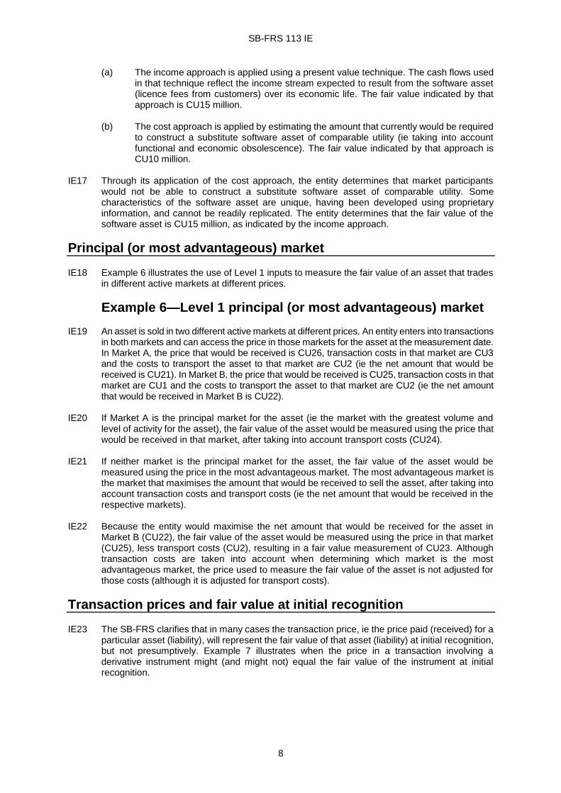
(a) The income approach is applied using a present value technique. The cash flows used in that technique reflect the income stream expected to result from the software asset (licence fees from customers) over its economic life. The fair value indicated by that approach is CU15 million.

(b) The cost approach is applied by estimating the amount that currently would be required

to construct a substitute software asset of comparable utility (ie taking into account functional and economic obsolescence). The fair value indicated by that approach is CU10 million.

IE17 Through its application of the cost approach, the entity determines that market participants

would not be able to construct a substitute software asset of comparable utility. Some characteristics of the software asset are unique, having been developed using proprietary information, and cannot be readily replicated. The entity determines that the fair value of the software asset is CU15 million, as indicated by the income approach.

Principal (or most advantageous) market IE18 Example 6 illustrates the use of Level 1 inputs to measure the fair value of an asset that trades

in different active markets at different prices.

Example 6—Level 1 principal (or most advantageous) market IE19 An asset is sold in two different active markets at different prices. An entity enters into transactions

in both markets and can access the price in those markets for the asset at the measurement date. In Market A, the price that would be received is CU26, transaction costs in that market are CU3 and the costs to transport the asset to that market are CU2 (ie the net amount that would be received is CU21). In Market B, the price that would be received is CU25, transaction costs in that market are CU1 and the costs to transport the asset to that market are CU2 (ie the net amount that would be received in Market B is CU22).

IE20 If Market A is the principal market for the asset (ie the market with the greatest volume and

level of activity for the asset), the fair value of the asset would be measured using the price that would be received in that market, after taking into account transport costs (CU24).

IE21 If neither market is the principal market for the asset, the fair value of the asset would be

measured using the price in the most advantageous market. The most advantageous market is the market that maximises the amount that would be received to sell the asset, after taking into account transaction costs and transport costs (ie the net amount that would be received in the respective markets).

IE22 Because the entity would maximise the net amount that would be received for the asset in

Market B (CU22), the fair value of the asset would be measured using the price in that market (CU25), less transport costs (CU2), resulting in a fair value measurement of CU23. Although transaction costs are taken into account when determining which market is the most advantageous market, the price used to measure the fair value of the asset is not adjusted for those costs (although it is adjusted for transport costs).

Transaction prices and fair value at initial recognition IE23 The SB-FRS clarifies that in many cases the transaction price, ie the price paid (received) for a

particular asset (liability), will represent the fair value of that asset (liability) at initial recognition, but not presumptively. Example 7 illustrates when the price in a transaction involving a derivative instrument might (and might not) equal the fair value of the instrument at initial recognition.

SB-FRS 113 IE

9

Example 7—Interest rate swap at initial recognition IE24 Entity A (a retail counterparty) enters into an interest rate swap in a retail market with Entity B

(a dealer) for no initial consideration (ie the transaction price is zero). Entity A can access only the retail market. Entity B can access both the retail market (ie with retail counterparties) and the dealer market (ie with dealer counterparties).

IE25 From the perspective of Entity A, the retail market in which it initially entered into the swap is

the principal market for the swap. If Entity A were to transfer its rights and obligations under the swap, it would do so with a dealer counterparty in that retail market. In that case the transaction price (zero) would represent the fair value of the swap to Entity A at initial recognition, ie the price that Entity A would receive to sell or pay to transfer the swap in a transaction with a dealer counterparty in the retail market (ie an exit price). That price would not be adjusted for any incremental (transaction) costs that would be charged by that dealer counterparty.

IE26 From the perspective of Entity B, the dealer market (not the retail market) is the principal market

for the swap. If Entity B were to transfer its rights and obligations under the swap, it would do so with a dealer in that market. Because the market in which Entity B initially entered into the swap is different from the principal market for the swap, the transaction price (zero) would not necessarily represent the fair value of the swap to Entity B at initial recognition. If the fair value differs from the transaction price (zero), Entity B applies SB-FRS 39 Financial Instruments: Recognition and Measurement or SB-FRS 109 Financial Instruments to determine whether it recognises that difference as a gain or loss at initial recognition.

Restricted assets IE27 The effect on a fair value measurement arising from a restriction on the sale or use of an asset

by an entity will differ depending on whether the restriction would be taken into account by market participants when pricing the asset. Examples 8 and 9 illustrate the effect of restrictions when measuring the fair value of an asset.

Example 8—Restriction on the sale of an equity instrument IE28 An entity holds an equity instrument (a financial asset) for which sale is legally or contractually

restricted for a specified period. (For example, such a restriction could limit sale to qualifying investors.) The restriction is a characteristic of the instrument and, therefore, would be transferred to market participants. In that case the fair value of the instrument would be measured on the basis of the quoted price for an otherwise identical unrestricted equity instrument of the same issuer that trades in a public market, adjusted to reflect the effect of the restriction. The adjustment would reflect the amount market participants would demand because of the risk relating to the inability to access a public market for the instrument for the specified period. The adjustment will vary depending on all the following:

(a) the nature and duration of the restriction; (b) the extent to which buyers are limited by the restriction (eg there might be a large

number of qualifying investors); and (c) qualitative and quantitative factors specific to both the instrument and the issuer.

Example 9—Restrictions on the use of an asset IE29 A donor contributes land in an otherwise developed residential area to a not-for-profit

neighbourhood association. The land is currently used as a playground. The donor specifies that the land must continue to be used by the association as a playground in perpetuity. Upon review of relevant documentation (eg legal and other), the association determines that the fiduciary responsibility to meet the donor’s restriction would not be transferred to market participants if the association sold the asset, ie the donor restriction on the use of the land is specific to the association. Furthermore, the association is not restricted from selling the land.

SB-FRS 113 IE

10

Without the restriction on the use of the land by the association, the land could be used as a site for residential development. In addition, the land is subject to an easement (ie a legal right that enables a utility to run power lines across the land). Following is an analysis of the effect on the fair value measurement of the land arising from the restriction and the easement:

(a) Donor restriction on use of land. Because in this situation the donor restriction on the

use of the land is specific to the association, the restriction would not be transferred to market participants. Therefore, the fair value of the land would be the higher of its fair value used as a playground (ie the fair value of the asset would be maximised through its use by market participants in combination with other assets or with other assets and liabilities) and its fair value as a site for residential development (ie the fair value of the asset would be maximised through its use by market participants on a stand-alone basis), regardless of the restriction on the use of the land by the association.

(b) Easement for utility lines. Because the easement for utility lines is specific to (ie a

characteristic of) the land, it would be transferred to market participants with the land. Therefore, the fair value measurement of the land would take into account the effect of the easement, regardless of whether the highest and best use is as a playground or as a site for residential development.

Measuring liabilities IE30 A fair value measurement of a liability assumes that the liability, whether it is a financial liability

or a non-financial liability, is transferred to a market participant at the measurement date (ie the liability would remain outstanding and the market participant transferee would be required to fulfil the obligation; it would not be settled with the counterparty or otherwise extinguished on the measurement date).

IE31 The fair value of a liability reflects the effect of non-performance risk. Non-performance risk

relating to a liability includes, but may not be limited to, the entity’s own credit risk. An entity takes into account the effect of its credit risk (credit standing) on the fair value of the liability in all periods in which the liability is measured at fair value because those that hold the entity’s obligations as assets would take into account the effect of the entity’s credit standing when estimating the prices they would be willing to pay.

IE32 For example, assume that Entity X and Entity Y each enter into a contractual obligation to pay

cash (CU500) to Entity Z in five years. Entity X has a AA credit rating and can borrow at 6 per cent, and Entity Y has a BBB credit rating and can borrow at 12 per cent. Entity X will receive about CU374 in exchange for its promise (the present value of CU500 in five years at 6 per cent). Entity Y will receive about CU284 in exchange for its promise (the present value of CU500 in five years at 12 per cent). The fair value of the liability to each entity (ie the proceeds) incorporates that entity’s credit standing.

IE33 Examples 10–13 illustrate the measurement of liabilities and the effect of non-performance risk

(including an entity’s own credit risk) on a fair value measurement.

Example 10—Structured note IE34 On 1 January 20X7 Entity A, an investment bank with a AA credit rating, issues a five-year fixed

rate note to Entity B. The contractual principal amount to be paid by Entity A at maturity is linked to an equity index. No credit enhancements are issued in conjunction with or otherwise related to the contract (ie no collateral is posted and there is no third-party guarantee). Entity A designated this note as at fair value through profit or loss. The fair value of the note (ie the obligation of Entity A) during 20X7 is measured using an expected present value technique. Changes in fair value are as follows:

(a) Fair value at 1 January 20X7. The expected cash flows used in the expected present

value technique are discounted at the risk-free rate using the government bond curve at 1 January 20X7, plus the current market observable AA corporate bond spread to

SB-FRS 113 IE

11

government bonds, if non-performance risk is not already reflected in the cash flows, adjusted (either up or down) for Entity A’s specific credit risk (ie resulting in a credit-adjusted risk-free rate). Therefore, the fair value of Entity A’s obligation at initial recognition takes into account non-performance risk, including that entity’s credit risk, which presumably is reflected in the proceeds.

(b) Fair value at 31 March 20X7. During March 20X7 the credit spread for AA corporate

bonds widens, with no changes to the specific credit risk of Entity A. The expected cash flows used in the expected present value technique are discounted at the risk-free rate using the government bond curve at 31 March 20X7, plus the current market observable AA corporate bond spread to government bonds, if non-performance risk is not already reflected in the cash flows, adjusted for Entity A’s specific credit risk (ie resulting in a credit-adjusted risk-free rate). Entity A’s specific credit risk is unchanged from initial recognition. Therefore, the fair value of Entity A’s obligation changes as a result of changes in credit spreads generally. Changes in credit spreads reflect current market participant assumptions about changes in non-performance risk generally, changes in liquidity risk and the compensation required for assuming those risks.

(c) Fair value at 30 June 20X7. As of 30 June 20X7 there have been no changes to the AA

corporate bond spreads. However, on the basis of structured note issues corroborated with other qualitative information, Entity A determines that its own specific creditworthiness has strengthened within the AA credit spread. The expected cash flows used in the expected present value technique are discounted at the risk-free rate using the government bond yield curve at 30 June 20X7, plus the current market observable AA corporate bond spread to government bonds (unchanged from 31 March 20X7), if non-performance risk is not already reflected in the cash flows, adjusted for Entity A’s specific credit risk (ie resulting in a credit-adjusted risk-free rate). Therefore, the fair value of the obligation of Entity A changes as a result of the change in its own specific credit risk within the AA corporate bond spread.

Example 11—Decommissioning liability IE35 On 1 January 20X1 Entity A assumes a decommissioning liability in a business combination.

The entity is legally required to dismantle and remove an offshore oil platform at the end of its useful life, which is estimated to be 10 years.

IE36 On the basis of paragraphs B23–B30 of the SB-FRS, Entity A uses the expected present value

technique to measure the fair value of the decommissioning liability. IE37 If Entity A was contractually allowed to transfer its decommissioning liability to a market

participant, Entity A concludes that a market participant would use all the following inputs, probability-weighted as appropriate, when estimating the price it would expect to receive:

(a) labour costs; (b) allocation of overhead costs; (c) the compensation that a market participant would require for undertaking the activity

and for assuming the risk associated with the obligation to dismantle and remove the asset. Such compensation includes both of the following:

(i) profit on labour and overhead costs; and (ii) the risk that the actual cash outflows might differ from those expected, excluding

inflation;

(d) effect of inflation on estimated costs and profits; (e) time value of money, represented by the risk-free rate; and

SB-FRS 113 IE

12

(f) non-performance risk relating to the risk that Entity A will not fulfil the obligation, including Entity A’s own credit risk.

IE38 The significant assumptions used by Entity A to measure fair value are as follows:

(a) Labour costs are developed on the basis of current marketplace wages, adjusted for expectations of future wage increases, required to hire contractors to dismantle and remove offshore oil platforms. Entity A assigns probability assessments to a range of cash flow estimates as follows:

Cash flow estimate (CU)

Probability assessment

Expected cash flows (CU)

100,000 25% 25,000

125,000 50% 62,500

175,000 25% 43,750

CU131,250

The probability assessments are developed on the basis of Entity A’s experience with fulfilling obligations of this type and its knowledge of the market.

(b) Entity A estimates allocated overhead and equipment operating costs using the rate it

applies to labour costs (80 per cent of expected labour costs). This is consistent with the cost structure of market participants.

(c) Entity A estimates the compensation that a market participant would require for

undertaking the activity and for assuming the risk associated with the obligation to dismantle and remove the asset as follows:

(i) A third-party contractor typically adds a mark-up on labour and allocated internal

costs to provide a profit margin on the job. The profit margin used (20 per cent) represents Entity A’s understanding of the operating profit that contractors in the industry generally earn to dismantle and remove offshore oil platforms. Entity A concludes that this rate is consistent with the rate that a market participant would require as compensation for undertaking the activity.

(ii) A contractor would typically require compensation for the risk that the actual cash

outflows might differ from those expected because of the uncertainty inherent in locking in today’s price for a project that will not occur for 10 years. Entity A estimates the amount of that premium to be 5 per cent of the expected cash flows, including the effect of inflation.

(d) Entity A assumes a rate of inflation of 4 per cent over the 10-year period on the basis

of available market data. (e) The risk-free rate of interest for a 10-year maturity on 1 January 20X1 is 5 per cent.

Entity A adjusts that rate by 3.5 per cent to reflect its risk of non-performance (ie the risk that it will not fulfil the obligation), including its credit risk. Therefore, the discount rate used to compute the present value of the cash flows is 8.5 per cent.

IE39 Entity A concludes that its assumptions would be used by market participants. In addition, Entity

A does not adjust its fair value measurement for the existence of a restriction preventing it from transferring the liability. As illustrated in the following table, Entity A measures the fair value of its decommissioning liability as CU194,879.

Expected cash flows (CU)

SB-FRS 113 IE

13

1 January 20X1

Expected labour costs 131,250

Allocated overhead and equipment costs (0.80 × CU131,250) 105,000

Contractor’s profit mark-up [0.20 × (CU131,250 + CU105,000)] 47,250

Expected cash flows before inflation adjustment 283,500

Inflation factor (4% for 10 years) 1.4802

Expected cash flows adjusted for inflation 419,637

Market risk premium (0.05 × CU419,637) 20,982

Expected cash flows adjusted for market risk 440,619

Expected present value using discount rate of 8.5% for 10 years 194,879

Example 12—Debt obligation: quoted price IE40 On 1 January 20X1 Entity B issues at par a CU2 million BBB-rated exchange-traded five-year

fixed rate debt instrument with an annual 10 per cent coupon. Entity B designated this financial liability as at fair value through profit or loss.

IE41 On 31 December 20X1 the instrument is trading as an asset in an active market at CU929 per

CU1,000 of par value after payment of accrued interest. Entity B uses the quoted price of the asset in an active market as its initial input into the fair value measurement of its liability (CU929 × [CU2 million ÷ CU1,000] = CU1,858,000).

IE42 In determining whether the quoted price of the asset in an active market represents the fair

value of the liability, Entity B evaluates whether the quoted price of the asset includes the effect of factors not applicable to the fair value measurement of a liability, for example, whether the quoted price of the asset includes the effect of a third-party credit enhancement if that credit enhancement would be separately accounted for from the perspective of the issuer. Entity B determines that no adjustments are required to the quoted price of the asset. Accordingly, Entity B concludes that the fair value of its debt instrument at 31 December 20X1 is CU1,858,000. Entity B categorises and discloses the fair value measurement of its debt instrument within Level 1 of the fair value hierarchy.

Example 13—Debt obligation: present value technique IE43 On 1 January 20X1 Entity C issues at par in a private placement a CU2 million BBB-rated five-

year fixed rate debt instrument with an annual 10 per cent coupon. Entity C designated this financial liability as at fair value through profit or loss.

IE44 At 31 December 20X1 Entity C still carries a BBB credit rating. Market conditions, including

available interest rates, credit spreads for a BBB-quality credit rating and liquidity, remain unchanged from the date the debt instrument was issued. However, Entity C’s credit spread has deteriorated by 50 basis points because of a change in its risk of non-performance. After taking into account all market conditions, Entity C concludes that if it was to issue the instrument at the measurement date, the instrument would bear a rate of interest of 10.5 per cent or Entity C would receive less than par in proceeds from the issue of the instrument.

IE45 For the purpose of this example, the fair value of Entity C’s liability is calculated using a present

value technique. Entity C concludes that a market participant would use all the following inputs (consistently with paragraphs B12–B30 of the SB-FRS) when estimating the price the market participant would expect to receive to assume Entity C’s obligation:

(a) the terms of the debt instrument, including all the following:

SB-FRS 113 IE

14

(i) coupon of 10 per cent; (ii) principal amount of CU2 million; and (iii) term of four years.

(b) the market rate of interest of 10.5 per cent (which includes a change of 50 basis points

in the risk of non-performance from the date of issue). IE46 On the basis of its present value technique, Entity C concludes that the fair value of its liability

at 31 December 20X1 is CU1,968,641. IE47 Entity C does not include any additional input into its present value technique for risk or profit

that a market participant might require for compensation for assuming the liability. Because Entity C’s obligation is a financial liability, Entity C concludes that the interest rate already captures the risk or profit that a market participant would require as compensation for assuming the liability. Furthermore, Entity C does not adjust its present value technique for the existence of a restriction preventing it from transferring the liability.

Measuring fair value when the volume or level of activity for an asset or a liability has significantly decreased IE48 Example 14 illustrates the use of judgement when measuring the fair value of a financial asset

when there has been a significant decrease in the volume or level of activity for the asset when compared with normal market activity for the asset (or similar assets).

Example 14—Estimating a market rate of return when the volume or level of activity for an asset has significantly decreased

IE49 Entity A invests in a junior AAA-rated tranche of a residential mortgage-backed security on 1

January 20X8 (the issue date of the security). The junior tranche is the third most senior of a total of seven tranches. The underlying collateral for the residential mortgage-backed security is unguaranteed non-conforming residential mortgage loans that were issued in the second half of 20X6.

IE50 At 31 March 20X9 (the measurement date) the junior tranche is now A-rated. This tranche of

the residential mortgage-backed security was previously traded through a brokered market. However, trading volume in that market was infrequent, with only a few transactions taking place per month from 1 January 20X8 to 30 June 20X8 and little, if any, trading activity during the nine months before 31 March 20X9.

IE51 Entity A takes into account the factors in paragraph B37 of the SB-FRS to determine whether

there has been a significant decrease in the volume or level of activity for the junior tranche of the residential mortgage-backed security in which it has invested. After evaluating the significance and relevance of the factors, Entity A concludes that the volume and level of activity of the junior tranche of the residential mortgage-backed security have significantly decreased. Entity A supported its judgement primarily on the basis that there was little, if any, trading activity for an extended period before the measurement date.

IE52 Because there is little, if any, trading activity to support a valuation technique using a market

approach, Entity A decides to use an income approach using the discount rate adjustment technique described in paragraphs B18–B22 of the SB-FRS to measure the fair value of the residential mortgage-backed security at the measurement date. Entity A uses the contractual cash flows from the residential mortgage-backed security (see also paragraphs 67 and 68 of the SB-FRS).

SB-FRS 113 IE

15

IE53 Entity A then estimates a discount rate (ie a market rate of return) to discount those contractual cash flows. The market rate of return is estimated using both of the following:

(a) the risk-free rate of interest. (b) estimated adjustments for differences between the available market data and the junior

tranche of the residential mortgage-backed security in which Entity A has invested. Those adjustments reflect available market data about expected non-performance and other risks (eg default risk, collateral value risk and liquidity risk) that market participants would take into account when pricing the asset in an orderly transaction at the measurement date under current market conditions.

IE54 Entity A took into account the following information when estimating the adjustments in

paragraph IE53(b):

(a) the credit spread for the junior tranche of the residential mortgage-backed security at the issue date as implied by the original transaction price.

(b) the change in the credit spread implied by any observed transactions from the issue

date to the measurement date for comparable residential mortgage-backed securities or on the basis of relevant indices.

(c) the characteristics of the junior tranche of the residential mortgage-backed security

compared with comparable residential mortgage-backed securities or indices, including all the following:

(i) the quality of the underlying assets, ie information about the performance of the

underlying mortgage loans such as delinquency and foreclosure rates, loss experience and prepayment rates;

(ii) the seniority or subordination of the residential mortgage-backed security

tranche held; and (iii) other relevant factors.

(d) relevant reports issued by analysts and rating agencies. (e) quoted prices from third parties such as brokers or pricing services.

IE55 Entity A estimates that one indication of the market rate of return that market participants would

use when pricing the junior tranche of the residential mortgage-backed security is 12 per cent (1,200 basis points). This market rate of return was estimated as follows:

(a) Begin with 300 basis points for the relevant risk-free rate of interest at 31 March 20X9. (b) Add 250 basis points for the credit spread over the risk-free rate when the junior tranche

was issued in January 20X8. (c) Add 700 basis points for the estimated change in the credit spread over the risk-free

rate of the junior tranche between 1 January 20X8 and 31 March 20X9. This estimate was developed on the basis of the change in the most comparable index available for that time period.

(d) Subtract 50 basis points (net) to adjust for differences between the index used to

estimate the change in credit spreads and the junior tranche. The referenced index consists of subprime mortgage loans, whereas Entity A’s residential mortgage-backed security consists of similar mortgage loans with a more favourable credit profile (making it more attractive to market participants). However, the index does not reflect an appropriate liquidity risk premium for the junior tranche under current market conditions. Thus, the 50 basis point adjustment is the net of two adjustments:

SB-FRS 113 IE

16

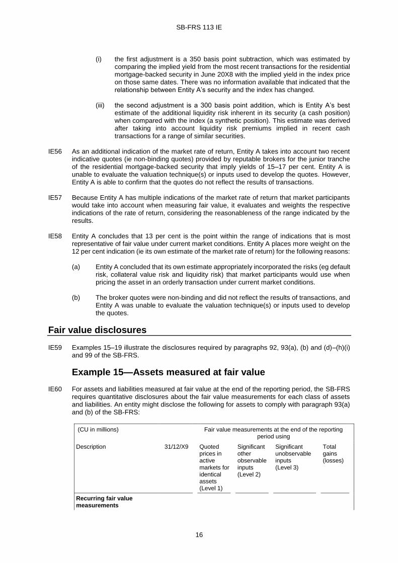
(i) the first adjustment is a 350 basis point subtraction, which was estimated by

comparing the implied yield from the most recent transactions for the residential mortgage-backed security in June 20X8 with the implied yield in the index price on those same dates. There was no information available that indicated that the relationship between Entity A’s security and the index has changed.

(iii) the second adjustment is a 300 basis point addition, which is Entity A’s best

estimate of the additional liquidity risk inherent in its security (a cash position) when compared with the index (a synthetic position). This estimate was derived after taking into account liquidity risk premiums implied in recent cash transactions for a range of similar securities.

IE56 As an additional indication of the market rate of return, Entity A takes into account two recent

indicative quotes (ie non-binding quotes) provided by reputable brokers for the junior tranche of the residential mortgage-backed security that imply yields of 15–17 per cent. Entity A is unable to evaluate the valuation technique(s) or inputs used to develop the quotes. However, Entity A is able to confirm that the quotes do not reflect the results of transactions.

IE57 Because Entity A has multiple indications of the market rate of return that market participants

would take into account when measuring fair value, it evaluates and weights the respective indications of the rate of return, considering the reasonableness of the range indicated by the results.

IE58 Entity A concludes that 13 per cent is the point within the range of indications that is most

representative of fair value under current market conditions. Entity A places more weight on the 12 per cent indication (ie its own estimate of the market rate of return) for the following reasons:

(a) Entity A concluded that its own estimate appropriately incorporated the risks (eg default

risk, collateral value risk and liquidity risk) that market participants would use when pricing the asset in an orderly transaction under current market conditions.

(b) The broker quotes were non-binding and did not reflect the results of transactions, and

Entity A was unable to evaluate the valuation technique(s) or inputs used to develop the quotes.

Fair value disclosures IE59 Examples 15–19 illustrate the disclosures required by paragraphs 92, 93(a), (b) and (d)–(h)(i)

and 99 of the SB-FRS.

Example 15—Assets measured at fair value IE60 For assets and liabilities measured at fair value at the end of the reporting period, the SB-FRS

requires quantitative disclosures about the fair value measurements for each class of assets and liabilities. An entity might disclose the following for assets to comply with paragraph 93(a) and (b) of the SB-FRS:

(CU in millions) Fair value measurements at the end of the reporting period using

Description 31/12/X9 Quoted prices in active markets for identical assets (Level 1)

Significant other observable inputs (Level 2)

Significant unobservable inputs (Level 3)

Total gains (losses)

Recurring fair value measurements

SB-FRS 113 IE

17

Trading equity securities(a):

Real estate industry 93 70 23

Oil and gas industry 45 45

Other 15 15

Total trading equity securities 153 130 23

Other equity securities:(a)

Financial services industry 150 150

Healthcare industry 163 110 53

Energy industry 32 32

Private equity fund investments(b) 25 25

Other 15 15

Total other equity securities 385 275 110

Debt securities:

Residential mortgage-backed securities 149 24 125

Commercial mortgage-backed securities 50 50

Collateralised debt obligations 35 35

Risk-free government securities 85 85

Corporate bonds 93 9 84

Total debt securities 412 94 108 210

continued...

SB-FRS 113 IE

18

...continued

(CU in millions) Fair value measurements at the end of the reporting period using

Description 31/12/X9

Quoted prices in active markets for identical assets (Level 1)

Significant other observable inputs (Level 2)

Significant unobservable inputs (Level 3)

Total gains (losses)

Hedge fund investments:

Equity long/short 55 55

Global opportunities 35 35

High-yield debt securities 90 90

Total hedge fund investments 180 90 90

Derivatives:

Interest rate contracts 57 57

Foreign exchange contracts 43 43

Credit contracts 38 38

Commodity futures contracts

78 78

Commodity forward contracts 20 20

Total derivatives 236 78 120 38

Investment properties:

Commercial—Asia 31 31

Commercial—Europe 27 27

Total investment properties 58 58

Total recurring fair value measurements 1,424 577 341 506

Non-recurring fair value measurements

Assets held for sale(c) 26 26 15

Total non-recurring fair value measurements 26 26 15

SB-FRS 113 IE

19

Example 16—Reconciliation of fair value measurements categorised within Level 3 of the fair value hierarchy

IE61 For recurring fair value measurements categorised within Level 3 of the fair value hierarchy,

the SB-FRS requires a reconciliation from the opening balances to the closing balances for each class of assets and liabilities. An entity might disclose the following for assets to comply with paragraph 93(e) and (f) of the SB-FRS:

SB-FRS 113 IE

Fair value measurements using significant unobservable inputs (Level 3)

(CU in millions)

Other equity securities

Debt securities Hedge fund investments

Derivatives Investment properties

Healthcare industry

Energy industry

Private equity fund

Residential mortgage-

backed securities

Commercial mortgage-

backed securities

Collateralised debt

obligations

High-yield debt

securities

Credit contracts

Asia Europe Total

Opening balance 49 28 20 105 39 25 145 30 28 26 495

Transfers into Level 3 60 (a), (b) 60

Transfers out of Level 3

(5) (b), (c)

(5)

Total gains or losses for the period

Included in profit or loss 5 (23) (5) (7) 7 5 3 1 (14)

Included in other comprehensive income 3 1 4

Purchases, issues, sales and settlements

Purchases 1 3 16 17 18 55

Issues

Sales (12) (62) (74)

Settlements (15) (15)

Closing balance 53 32 25 125 50 35 90 38 31 27 506

Change in unrealised gains or losses for the period included in profit or loss for assets held at the end of the reporting period 5 (3) (5) (7) (5) 2 3 1

(9)

continued...

SB-FRS 113 IE

21

...continued

(a) Transferred from Level 2 to Level 3 because of a lack of observable market data, resulting from a decrease in market activity for the securities.

(b) The entity's policy is to recognise transfers into and transfers out of Level 3 as of the date of the event or change in circumstances that caused the transfer.

(c) Transferred from Level 3 to Level 2 because observable market data became available for the securities.

(Note: A similar table would be presented for liabilities unless another format is deemed more appropriate by the entity.)

SB-FRS 113 IE

IE62 Gains and losses included in profit or loss for the period (above) are presented in financial income and in non-financial income as follows:

(CU in millions)

Financial income

Non-financial income

Total gains or losses for the period included in profit or loss

(18)

4

Change in unrealised gains or losses for the period included in profit or loss for assets held at the end of the reporting period

(13)

4


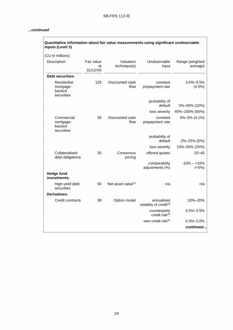
Example 17—Valuation techniques and inputs IE63 For fair value measurements categorised within Level 2 and Level 3 of the fair value hierarchy,

the SB-FRS requires an entity to disclose a description of the valuation technique(s) and the inputs used in the fair value measurement. For fair value measurements categorised within Level 3 of the fair value hierarchy, information about the significant unobservable inputs used must be quantitative. An entity might disclose the following for assets to comply with the requirement to disclose the significant unobservable inputs used in the fair value measurement in accordance with paragraph 93(d) of the SB-FRS:

SB-FRS 113 IE

23

Quantitative information about fair value measurements using significant unobservable inputs (Level 3)

(CU in millions)

Description Fair value at

31/12/X9

Valuation technique(s)

Unobservable input

Range (weighted average)

Other equity securities:

Healthcare industry

53 Discounted cash flow

weighted average cost of capital

7%–16% (12.1%)

long-term revenue growth rate

2%–5% (4.2%)

long-term pre-tax operating margin

3%–20% (10.3%)

discount for lack of marketability(a)

5%–20% (17%)

control premium(a) 10%–30% (20%)

Market comparable companies

EBITDA multiple(b) 10–13 (11.3)

revenue multiple(b) 1.5–2.0 (1.7)


5%–20% (17%)


Energy industry 32 Discounted cash flow

weighted average cost of capital

8%–12% (11.1%)

long-term revenue growth rate

3%–5.5% (4.2%)

long-term pre-tax operating margin

7.5%–13% (9.2%)


5%–20% (10%)


Market comparable companies

EBITDA multiple(b) 6.5–12 (9.5)

revenue multiple(b) 1.0–3.0 (2.0)


5%–20% (10%)


Private equity fund investments

25 Net asset value(c) n/a n/a

continued...

SB-FRS 113 IE

24

...continued

Quantitative information about fair value measurements using significant unobservable inputs (Level 3)

(CU in millions)


31/12/X9


Unobservable input


Debt securities:

Residential mortgage-backed securities


constant prepayment rate

3.5%–5.5% (4.5%)

probability of default

5%–50% (10%)

loss severity 40%–100% (60%)

Commercial mortgage-backed securities


constant prepayment rate

3%–5% (4.1%)

probability of default

2%–25% (5%)

loss severity 10%–50% (20%)

Collateralised debt obligations

35 Consensus pricing

offered quotes 20–45

comparability adjustments (%)

-10% – +15% (+5%)

Hedge fund investments:

High-yield debt securities

90 Net asset value(c) n/a n/a

Derivatives:

Credit contracts 38 Option model annualised volatility of credit(d)

10%–20%

counterparty credit risk(e)

0.5%–3.5%

own credit risk(e) 0.3%–2.0%

continued...

SB-FRS 113 IE

25

...continued

Quantitative information about fair value measurements using significant unobservable inputs (Level 3) (CU in millions)


31/12/X9


Unobservable input


Investment properties:

Commercial—Asia


long-term net operating income

margin

18%–32% (20%)

cap rate 0.08–0.12 (0.10)

Market comparable

approach

price per square metre (USD)

$3,000–$7,000 ($4,500)

Commercial—Europe


long-term net operating income

margin

15%–25% (18%)

cap rate 0.06–0.10 (0.08)

Market comparable

approach

price per square metre (EUR)

€4,000–€12,000 (€8,500)


(c) The entity has determined that the reported net asset value represents fair value at the end of the reporting period.

(d) Represents the range of the volatility curves used in the valuation analysis that the entity has determined market participants would use when the pricing contracts.

(e) Represents the range of the credit default swap spread curves used in the valuation analysis that the entity has determined market participants would use when pricing the contracts.

IE64 In addition, an entity should provide additional information that will help users of its financial

statements to evaluate the quantitative information disclosed. An entity might disclose some or all the following to comply with paragraph 92 of the SB-FRS:

(a) the nature of the item being measured at fair value, including the characteristics of the

item being measured that are taken into account in the determination of relevant inputs. For example, for residential mortgage-backed securities, an entity might disclose the following:

(i) the types of underlying loans (eg prime loans or sub-prime loans) (ii) collateral (iii) guarantees or other credit enhancements (iv) seniority level of the tranches of securities (v) the year of issue (vi) the weighted-average coupon rate of the underlying loans and the securities

SB-FRS 113 IE

26

(vii) the weighted-average maturity of the underlying loans and the securities (viii) the geographical concentration of the underlying loans (ix) information about the credit ratings of the securities.

(b) how third-party information such as broker quotes, pricing services, net asset values

and relevant market data was taken into account when measuring fair value.

Example 18—Valuation processes IE65 For fair value measurements categorised within Level 3 of the fair value hierarchy, the SB-FRS

requires an entity to disclose a description of the valuation processes used by the entity. An entity might disclose the following to comply with paragraph 93(g) of the SB-FRS:

(a) for the group within the entity that decides the entity’s valuation policies and

procedures:

(i) its description; (ii) to whom that group reports; and (iii) the internal reporting procedures in place (eg whether and, if so, how pricing, risk

management or audit committees discuss and assess the fair value measurements);

(b) the frequency and methods for calibration, back testing and other testing procedures of

pricing models; (c) the process for analysing changes in fair value measurements from period to period; (d) how the entity determined that third-party information, such as broker quotes or pricing

services, used in the fair value measurement was developed in accordance with the SB-FRS; and

(e) the methods used to develop and substantiate the unobservable inputs used in a fair

value measurement.

Example 19—Information about sensitivity to changes in significant unobservable inputs

IE66 For recurring fair value measurements categorised within Level 3 of the fair value hierarchy,

the SB-FRS requires an entity to provide a narrative description of the sensitivity of the fair value measurement to changes in significant unobservable inputs and a description of any interrelationships between those unobservable inputs. An entity might disclose the following about its residential mortgage-backed securities to comply with paragraph 93(h)(i) of the SB-FRS:

The significant unobservable inputs used in the fair value measurement of the entity’s residential mortgage-backed securities are prepayment rates, probability of default and loss severity in the event of default. Significant increases (decreases) in any of those inputs in isolation would result in a significantly lower (higher) fair value measurement. Generally, a change in the assumption used for the probability of default is accompanied by a directionally similar change in the assumption used for the loss severity and a directionally opposite change in the assumption used for prepayment rates.

SB-FRS 113 IE

27

Appendix Amendments to guidance on other SB-FRSs The following amendments to guidance on other SB-FRSs are necessary in order to ensure consistency with SB-FRS 113 Fair Value Measurement and the related amendments to other SB-FRSs. Amended paragraphs are shown with new text underlined and deleted text struck through.

* * * * *

The amendments contained in this appendix when SB-FRS 113 was issued in 2011 have been incorporated into the guidance on the relevant SB-FRSs published in this volume.

Documents

Fair Value Measurement Illustrative Examples - …€¦ · advanced stage of development that would compete with the project if completed and the project would be expected to improve