FAIR ALLOCATION OF A WIRELESS FADING CHANNEL: AN AUCTION APPROACH

FAIR ALLOCATION OF A WIRELESS FADING CHANNEL:AN AUCTION APPROACH

JUN SUN AND EYTAN MODIANO ∗

Abstract. We study the use of auction algorithm in allocating a wireless fadingchannel among a set of non-cooperating users in both downlink and uplink communi-cation scenarios. For the downlink case, we develop a novel auction-based algorithm toallow users to fairly compete for a wireless fading channel. We use the all-pay auctionmechanism whereby user bid for the channel, during each time-slot, based on the fadestate of the channel, and the user that makes the higher bid wins use of the channel.Under the assumption that each user has a limited budget for bidding, we show theexistence of a unique Nash equilibrium strategy. We show that the strategy achievesa throughput allocation for each user that is proportional to the user’s budget and es-tablish that the aggregate throughput received by the users using the Nash equilibriumstrategy is at least 3/4 of what can be obtained using an optimal centralized allocationscheme that does not take fairness into account. We also provide a distributed algorithmthat enables user’s bidding strategy to converge to the Nash equilibrium strategy.

For the uplink case, we present a game-theoretical model of a wireless communicationsystem with multiple competing users sharing a multiaccess fading channel. With aspecified capture rule and a limited amount of energy available, a user opportunisticallyadjusts its transmission power based on its own channel state to maximize the user’sown individual throughput. We derive an explicit form of the Nash equilibrium powerallocation strategy. Furthermore, this Nash equilibrium power allocation strategy isunique under certain capture rule. We also quantify the loss of efficiency in throughputdue to user’s selfish behavior. Moreover, as the number of users in the system increases,the total system throughput obtained by using a Nash equilibrium strategy approachesthe maximum attainable throughput.

Key words. Stochastic processes, Mathematical programming/optimization.

AMS(MOS) subject classifications. Primary 91A80, 91A10, 93E03, 93A14.

1. Introduction. The limited bandwidth and high demand in a com-munication network necessitate a systematic procedure in place for fair al-location. This is where the economic theory of pricing and auction can beapplied in the field of communications and networks research, for pricingand auction are natural ways to allocate resources with limited supply. Re-cently, in the networks area, much work is done to address the allocationof a limited resource in a complex, large scaled system such as the internet.They approach the problem from a classical economic perspective whereusers have utility functions and cost functions, both measured in the samemonetary unit. Pricing is used as a tool to balance users’ demand forbandwidth.

Here, we are interested in solving a specific engineering problem ofscheduling transmission among a set of users while achieving fairness in

∗Laboratory for Information and Decision Systems, Massachusetts Institute of Tech-nology, Cambridge, MA 02139. The work was supported by NASA Space Communica-tion Project grant number NAG3-2835.

1

2 JUN SUN AND EYTAN MODIANO

a specific wireless environment. We use game theoretical concepts suchas Nash equilibrium as a tool for modelling the interaction among users.Both the objective and the constraint of the optimization problem thateach user faces have physical meanings based on underlying system. Ourfocus in this paper will be on the use of the all-pay auction in allocating awireless fading channel for both the uplink and the downlink.

A fundamental characteristic of a wireless network is that the channelover which communication takes place is often time-varying. This variationof the channel quality is due to constructive and destructive interferencebetween multipaths and shadowing effects (fading). In a single cell with onetransmitter (base station or satellite) and multiple users communicatingthrough time-varying fading channels, the transmitter can send data athigher rates to users with better channels. In time slotted system such asthe HDR system, time slots are allocated among users according to theirchannel qualities.

The problem of resource allocation in wireless networks has receivedmuch attention in recent years. In [1] the authors try to maximize thedata throughput of an energy and time constrained transmitter sendingover a fading channel. A dynamic programming formulation that leads toan optimal transmission schedule is presented. Other works address thesimilar problem, without consideration to fairness, include [7] and [8]. In[5], the authors consider scheduling policies for maxmin fairness allocationof bandwidth, which maximizes the allocation for the most poorly treatedsessions while not wasting any network resources, in wireless ad-hoc net-works. In [14], the authors designed a scheduling algorithm that achievesproportional fairness, a notion of fairness originally proposed by Kelly [6].In [9], the authors present a slot allocation scheme that maximizes expectedsystem performance subject to the constraint that each user gets a fixedfraction of time slots. The authors did not use a formal notion of fairness,but argue that their system can explicitly set the fraction of time assignedto each user. Hence, while each user may get to use the channel an equalfraction of the time, the resulting throughput obtained by each user maybe vastly different.

The following simple example illustrates the different allocations thatmay result from the different notions of fairness. We consider the com-munication system with one transmitter and two users, A and B, and theallocations that use different notions of fairness discussed in the previousparagraph. We assume that the throughput is proportional to the thechannel condition. The channel coefficient, which is a quantitative mea-sure of the channel condition ranging from 0 to 1 with 1 as the best channelcondition, for user A and user B in the two time slots are (0.1, 0.2) and(0.3, 0.9) respectively. The throughput result for each individual user andfor total system under different notions of fairness constraint are given inTable I. When there is no fairness constraint, to maximize the total systemthroughput would require the transmitter to allocate both time slots to user

FAIR ALLOCATION OF A WIRELESS FADING CHANNEL 3

B. To achieve maxmin fair allocation, the transmitter would allocate slotone to user B and slot two to user A, thus resulting in a total throughput of0.5. If the transmitter wants to maximize the total throughput subject tothe constraint that each user gets one time slot (i.e., the approach of [9]),the resulting allocation, denoted as time fraction fair, is to give user A slotone and user B slot two. As a result, the total throughput is 1.0. In the

Throughput Throughput Total

for user A for user B throughput

No fair constraint 0 1.2 1.2Maxmin fair 0.2 0.3 0.5Time fraction 0.1 0.9 1.0

Table 1Throughput results using different notions of fairness.

above example, the transmitter selects an allocation to ensure an artificiallychosen notion of fairness. From Table I, we can see that from the user’sperspective, no notion is truly fair as both users want slot two. In order toresolve this conflict, we use a new approach which allows users to competefor time slots. In this way, each user is responsible for its own action andits resulting throughput. We call the fraction of bandwidth received byeach user competitive fair. Using this notion of competitive fairness, theresulting throughput obtained for each user can serve as a reference pointfor comparing various other allocations. Moreover, the competitive fair al-location scheme can provide fundamental insight into the design of a fairscheduler that make sense.

In our model, users compete for time-slots. For each time-slot, eachuser has a different valuation (i.e., its own channel condition). And eachuser is only interested in getting a higher throughput for itself. Naturally,these characteristics give rise to an auction. In this paper we consider theall-pay auction mechanism. Using the all-pay auction mechanism, userssubmit a “bid” for the time-slot and the transmitter allocates the slotto the user that made the highest bid. Moreover, in the all-pay auctionmechanism, the transmitter gets to keep the bids of all users (regardlessof whether or not they win the auction). Each user is assumed to have aninitial amount of money. The money possessed by each user can be viewedas fictitious money that serves as a mechanism to differentiate the QoSgiven to the various users. This fictitious money, in fact, could correspondto a certain QoS for which the user paid in real money. As for the solutionof the slot auction game, we use the concept of Nash equilibrium, which isa set of strategies (one for each player) from which there are no profitableunilateral deviation.

In the downlink communication scenario, we consider a communica-tion system with one transmitter and two users. For each time slot, channel


states are independent and identically distributed with known probabilitydistribution. Each user wants to maximize its own expected total through-put subject to an average money constraint.

We have the following main results for the downlink case:• We find a unique Nash equilibrium when both channel states are

uniformly distributed over [0, 1].• We show that the Nash equilibrium strategy pair provides an al-

location scheme that is fair in the sense that the price per unit ofthroughput is the same for both users.

• We show that the Nash equilibrium strategy of this auction leads toan allocations at which total throughput is no worse than 3/4 of thethroughput obtained by an algorithm that attempts to maximizetotal system throughput without a fairness constraint.

• We provide an estimation algorithm that enables users to accu-rately estimate the amount of money possessed by their opponentso that users do not need prior knowledge of each other’s money.

The all-pay auction can be used to model the uplink power allocationas well. In the second part of this paper, we present a distributed uplinkpower allocation scheme that based on the all-pay auction. Specifically, weconsider a communication system consisting of multiple users competing toaccess a satellite, or a base-station. Each user has an average power con-straint. Time is slotted. During each time slot, each user chooses a powerlevel for transmission based on the channel state of current slot, which isonly known to itself. Depending on the capture model and the receivedpower of that user’s signal, a transmitted packet may be captured even ifmultiple users are transmitting at the same slot. If the objective of eachuser in the system is to find a power allocation strategy that maximizes itsprobability of getting captured based its average power constraint, we havea power allocation game that resembles the all-pay auction. Comparingwith the all-pay auction, the average power constraint in the power alloca-tion game corresponds to the average money constraint and transmissionpower corresponds to money. Both power and money is taken away oncea bidding or a transmission is taken place. In this uplink scenario, usingthe technique to solve for Nash equilibrium in the all-pay auction, we geta similar Nash equilibrium strategy in the uplink game.

The game theoretical formulation of the uplink power allocation prob-lem stems from the desire for a distributive algorithm in a wireless uplink.Due to the variation of channel quality in a fading channel, one can ex-ploit the channel variation opportunistically by allowing the user with bestchannel condition to transmit, which require the presence of a centralizedscheduler who knows each user’s channel condition. As the number of usersin the network increases, the delay in conveying user’s channel conditionsto the scheduler will limit the system’s performance. Hence, a distributivemulti-access scheme with no centralized scheduler becomes an attractivealternative. However, in a distributive environment, users may want to


change their communication protocols in order to improve their own per-formance, making it impossible to ensure a particular algorithm will beadopted by all users in the network. Rather than following some mandatedalgorithm, in this paper users are assumed to act selfishly (i.e., choose theirown power allocation strategies) to further their own individual interests.

With each user wants to maximize its own expected throughput, weobtain a Nash equilibrium power allocation strategy which determines theoptimal transmission power control strategy for each user. The obtainedoptimal power control strategy specifies how much power a user needs touse to maximize its own throughput for any possible channel state. Usersget different average throughput based on their average power constraint.Hence, this transmission scheme can be viewed as mechanism for providingquality of service (QoS) differentiation; whereby users are given differentenergy for transmission. The obtained Nash equilibrium power allocationstrategy is unique under certain capture rule. When all users have the sameenergy constraint, we obtained a symmetric Nash equilibrium.

Due to the selfish behavior of individual users, the overall systemthroughput will be less than that of a system where users employ the samemandated algorithm. This loss in efficiency is also quantified. In the multi-ple users’ case, as the number of user in the system increases, the symmetricNash equilibrium strategy approaches the optimal algorithm specified bya system designer (i.e., algorithm that results in the largest total systemthroughput). In this case, there is no loss of efficiency when users employthe symmetric Nash equilibrium.

Game theoretical approaches to resource allocation problems havebeen explored by many researchers recently (e.g., [2][19]). In [2], the au-thors consider a resource allocation problem for a wireless channel, withoutfading, where users have different utility values for the channel. They showthe existence of an equilibrium pricing scheme where the transmitter at-tempts to maximize its revenue and the users attempt to maximize theirindividual utilities. In [19], the authors explore the properties of a conges-tion game where users of a congested resource anticipate the effect of theiraction on the price of the resource. Again, the work of [19] focuses on awireline channel without the notion of wireless fading. Our work attemptsto apply game theory to the allocation of a wireless fading channel. In par-ticular, we show that auction algorithms are well suited for achieving fairallocation in this environment. Other papers dealing with the applicationof game theory to resource allocation problems include [3][23][24].

This paper is organized as follows. In Section 2, we describe the don-wlink communication system and the Nash equilibrium bidding strategy.Section 2.1 presents the problem formulation for the downlink case. InSection 2.2, the unique Nash equilibrium strategy pair and the resultingthroughput for each user are provided for the case that each user can useonly one bidding function. In Section 2.3, we show the unique Nash equi-librium strategy pair for the case that each user can use multiple bidding


functions. In Section 2.4, we compare the throughput results of the Nashequilibrium strategy with two other centralized allocation algorithms. InSection 2.5, an estimation algorithm that enables the users to estimatethe amount of money possessed by their opponent is developed. Section3 presents the Nash equilibrium power allocation function for a uplinkrandom access system. Section 3.1 describe the uplink communication sce-nario. In Section 3.2, the Nash equilibrium power allocation strategy isobtained for the two users case. In Section 3.3, we present a symmet-ric Nash equilibrium power allocation function for multiple users with thesame average power constraint. Finally, Section 4 concludes the paper.

2. Downlink Transmission.

2.1. Downlink Problem Formulation. We consider a communica-tion environment with a single transmitter sending data to two users overtwo different fading channels. We assume that there is always data to besent to the users. Time is assumed to be discrete, and the channel state fora given channel changes according to a known probabilistic model indepen-dently over time. The two channels are also assumed to be independent ofeach other. The transmitter can transmit to only one user during a partic-ular slot with a constant power P . The channel fade state thus determinesthe throughput that can be obtained.

For a given power level, we assume for simplicity that the throughput isa linear function of the channel state. This can be justified by the Shannoncapacity at low signal-to-noise ratio, or by using a fixed modulation scheme[1]. For general throughput function, the method used in this paper appliesas well. Let Xi be a random variable denoting the channel state for thechannel between the transmitter and user i, i = 1, 2. When transmittingto user i, the throughput will then be P · Xi. Without loss of generality,we assume P = 1 throughout this paper.

We now describe the all-pay auction rule used in this paper. Let αand β be the average amount of money available to user 1 and user 2respectively during each time slot. We assume that the values of α and βare known to both users. Both users know the distribution of X1 and X2.We also assume that the exact value of the channel state Xi is revealed touser i only at the beginning of each time slot. During each time slot, thefollowing actions take place:

1. Each user submits a bid according to the channel condition re-vealed to it.

2. The transmitter chooses the one with higher bid to transmit.3. Once a bid is submitted by the user, it is taken by the transmitter

regardless of whether the user gets the slot or not, i.e., no refundfor the one who loses the bid.

The formulation of our auction is different from the type of auctionused in economic theory in several ways. First, we look at a case wherethe number of object in the auction goes to infinity. While in the current


auction research, the number of object is finite [20][21][22]. Second, in ourauction formulation, the money used for bidding does not have a directconnection with the value of the time slot. Money is merely a tool for usersto compete for time slots, and it has no value after the auction. Therefore,it is desirable for each user to spend all of its money. However, in auctiontheory, an object’s value is measured in the same unit as the money usedin the bidding process, hence their objective is to maximize the differencebetween the object’s value and its cost. Lastly, in our formulation, thevaluation of each commodity (time-slot) changes due to the fading channelmodel; a notion that is not common in economic theory.

Besides the all-pay auction, first-price auction and second-price auc-tion are two other commonly used auction mechanisms. In the first-priceauction, each bidder submits a single bid without seeing the others’ bids,and the object is sold to the bidder who makes the highest bid. The winnerpays its bid. In the second price auction, each user independently submitsa single bid without seeing the others’ bids, and the object is sold to thebidder who makes the highest bid. However, the price it pays is the sec-ond -highest bidder’s bid [20]. We choose to use the all-pay auction in thispaper to illustrate the auction approach to resource allocation in wirelessnetworks. We believe that other auction mechanisms can be similarly ap-plied and their application to the wireless channel allocation problem is adirection for future research.

The objective for each user is to design a bidding strategy, whichspecifies how a user will act in every possible distinguishable circumstance,to maximize its own expected throughput per time slot subject to theexpected or average money constraint. Once a user, say user 1, choosesa function, say f

(i)1 , for its strategy in the ith slot, it bids an amount of

money equal to f(i)1 (x) when it sees its channel condition in the ith slot is

X1 = x.Formally, let F1 and F2 be the set of continuous and bounded real-

valued functions with finite first and second derivative over the support ofX1 and X2 respectively. Then, the strategy space for user 1, say S1, anduser 2, say S2, are defined as follows:

S1 ={

f(1)1 , · · · , f

(n)1 ∈ F1

∣∣∣ 1n

n∑

i=1

E[f (i)1 (X1)] = α

}

S2 ={

f(1)2 , · · · , f

(n)2 ∈ F2

∣∣∣ 1n

n∑

i=1

E[f (i)2 (X2)] = β

} (2.1)

For each user, a strategy is a sequence of bidding functions f (1), · · · , f (n).Without loss of generality, we restrict each user to have n different biddingfunctions, where n can be chosen as an arbitrarily large number. Notethat users choose a strategy for a block of n time slots instead of just for a


single time slot, one bidding function for each slot. In order to maximizethe overall throughput (over infinite horizon), each user chooses biddingfunctions to maximize the expected total throughput over this block of n

slots. The term E[f (i)1 (X1)] denotes the expected amount of money spent

by user 1 if it uses bidding function f(i)1 for the ith slot in the block.

We first consider a special class of strategies in which each user canuse only a single bidding function. More specifically, by setting f1 = f

(1)1 =

· · · = f(n)1 and f2 = f

(1)2 = · · · = f

(n)2 , we have the following:

S1 ={

f1 ∈ F1

∣∣∣ E[f1(X1)] = α}

S2 ={

f2 ∈ F2

∣∣∣ E[f2(X2)] = β} (2.2)

By considering first the set of strategies in S1 and S2, we are able to findthe Nash equilibrium strategy pair within the set S1 and S2.

Given a strategy pair (f1, f2), where f1 ∈ S1 and f2 ∈ S2, the expectedthroughput or payoff function for user 1 is defined as the following assumingthe constant power P = 1:

G1(α, β) = EX1,X2 [X1 · 1f1(X1)≥f2(X2)] (2.3)

where

1f1(X1)≥f2(X2) ={

1 if f1(X1) ≥ f2(X2)0 otherwise

Similarly, the throughput function for user 2 assuming P = 1:

G2(α, β) = EX1,X2 [X2 · 1f2(X2)>f1(X1)] (2.4)

Throughout this paper, for simplicity, we let the channel state Xi beuniformly distributed over [0, 1]. However, our approach can be extendedto the case where the channel state has a general distribution. Due to spacelimitations, we omit the more complex analysis for general channel statedistribution.

2.2. Unique Nash equilibrium strategy with a single biddingfunction. We present in this section a unique Nash equilibrium strategypair (f∗1 , f∗2 ). A strategy pair (f∗1 , f∗2 ) is said to be in Nash equilibrium iff∗1 is the best response for user 1 to user 2’s strategy f∗2 , and f∗2 is the bestresponse for user 2 to user 1’s strategy f∗1 . We consider here the case whereboth users choose their strategies from the strategy space S1 and S2 (i.e.,the single bidding function strategy) and the value of α and β are knownto both users.

To get the Nash equilibrium strategy pair, we first argue that an equi-librium bidding function must be nondecreasing. To see this, consider an


arbitrary bidding function f such that f(a) > f(b) for some a < b. If user1 chooses f as its bidding function, user 1 will be better off if it bids f(b)when the channel state is a and f(a) when the channel state is b. This way,its odds of winning the slot when the channel state is b, which is more valu-able to it, will be higher than before, and it has an incentive to change itsstrategy (i.e., f is not an equilibrium strategy). Hence, we conclude that,for each user, an equilibrium bidding function must be nondecreasing.

We further restrict users’ bidding functions to be strictly increasingfor technical reason which will be explained later. There is no loss of gen-erality in this assumption because any continuous, bounded, nondecreasingfunction can be approximated by a strictly increasing function arbitrarilyclosely.

Next, we show some useful properties associated with the equilibriumstrategy pair (f∗1 , f∗2 ).

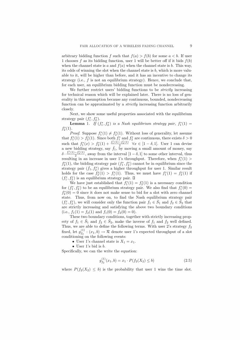
Lemma 1. If (f∗1 , f∗2 ) is a Nash equilibrium strategy pair, f∗1 (1) =f∗2 (1).

Proof. Suppose f∗1 (1) 6= f∗2 (1). Without loss of generality, let assumethat f∗1 (1) > f∗2 (1). Since both f∗1 and f∗2 are continuous, there exists δ > 0such that f∗1 (x) > f∗2 (1) + f∗1 (1)−f∗2 (1)

2 ∀x ∈ [1 − δ, 1]. User 1 can devisea new bidding strategy, say f1, by moving a small amount of money, sayδ · f∗1 (1)−f∗2 (1)

2 , away from the interval [1− δ, 1] to some other interval, thusresulting in an increase in user 1’s throughput. Therefore, when f∗1 (1) >f∗2 (1), the bidding strategy pair (f∗1 , f∗2 ) cannot be in equilibrium since thestrategy pair (f1, f

∗2 ) gives a higher throughput for user 1. Similar result

holds for the case f∗2 (1) > f∗1 (1). Thus, we must have f∗1 (1) = f∗2 (1) if(f∗1 , f∗2 ) is an equilibrium strategy pair.

We have just established that f∗1 (1) = f∗2 (1) is a necessary conditionfor (f∗1 , f∗2 ) to be an equilibrium strategy pair. We also find that f∗1 (0) =f∗2 (0) = 0 since it does not make sense to bid for a slot with zero channelstate. Thus, from now on, to find the Nash equilibrium strategy pair(f∗1 , f∗2 ), we will consider only the function pair f1 ∈ S1 and f2 ∈ S2 thatare strictly increasing and satisfying the above two boundary conditions(i.e., f1(1) = f2(1) and f1(0) = f2(0) = 0).

These two boundary conditions, together with strictly increasing prop-erty of f1 ∈ S1 and f2 ∈ S2, make the inverse of f1 and f2 well defined.Thus, we are able to define the following terms. With user 2’s strategy f2

fixed, let g(1)f2

: (x1, b) → R denote user 1’s expected throughput of a slotconditioning on the following events:

• User 1’s channel state is X1 = x1.• User 1’s bid is b.

Specifically, we can the write the equation:

g(1)f2

(x1, b) = x1 · P (f2(X2) ≤ b) (2.5)

where P (f2(X2) ≤ b) is the probability that user 1 wins the time slot.


Consequently, using a strategy f1, user 1’s throughput is given by:

G1(α, β) =∫ 1

0

g(1)f2

(x1, f1(x1)) · pX1(x1) dx1 =∫ 1

0

g(1)f2

(x1, f1(x1)) dx1.

(2.6)

where the last equality results from the uniform distribution assumption.With user 1’s strategy f1 fixed, similar terms for user 2 can be defined.

g(2)f1

(x2, b) = x2 · P (f1(X1) ≤ b)

Then, user 2’s throughput is given by:

G2(α, β) =∫ 1

0

g(2)f1

(x2, f2(x2)) · pX2(x2) dx2 =∫ 1

0

g(2)f1

(x2, f2(x2)) dx2.

(2.7)

Due to the uniformly distributed channel state, P (f2(X2) ≤ b) is given by

P (f2(X2) ≤ b) = P (X2 ≤ f−12 (b)) = f−1

2 (b)

where f−12 is well defined. Thus, we can rewrite Eq. (3.4) as

g(1)f2

(x1, b) = x1 · f−12 (b).

Hence we have,

G1(α, β) =∫ 1

0

x1 · f−12 (f1(x1)) dx1 (2.8)

G2(α, β) =∫ 1

0

x2 · f−11 (f2(x2)) dx2 (2.9)

The following lemma gives a necessary and sufficient condition of a

Nash equilibrium strategy pair. For convenience, we denote∂g

(1)f2

(x1,b)

∂b |||b=b∗

(i.e., the marginal gain at b = b∗) as Dg(1)f2

(x1, b∗).

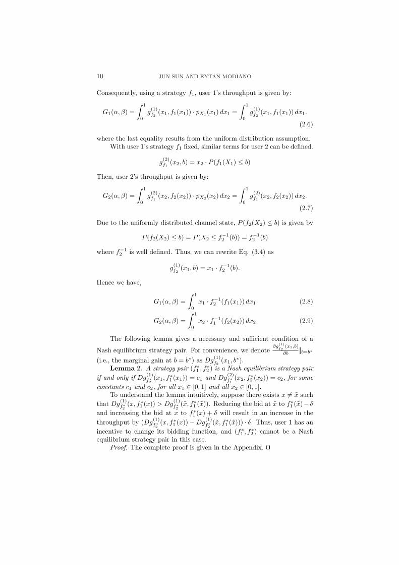
Lemma 2. A strategy pair (f∗1 , f∗2 ) is a Nash equilibrium strategy pairif and only if Dg

(1)f∗2

(x1, f∗1 (x1)) = c1 and Dg

(2)f∗1

(x2, f∗2 (x2)) = c2, for some

constants c1 and c2, for all x1 ∈ [0, 1] and all x2 ∈ [0, 1].To understand the lemma intuitively, suppose there exists x 6= x such

that Dg(1)f∗2

(x, f∗1 (x)) > Dg(1)f∗2

(x, f∗1 (x)). Reducing the bid at x to f∗1 (x)− δ

and increasing the bid at x to f∗1 (x) + δ will result in an increase in thethroughput by (Dg

(1)f∗2

(x, f∗1 (x))−Dg(1)f∗2

(x, f∗1 (x))) · δ. Thus, user 1 has anincentive to change its bidding function, and (f∗1 , f∗2 ) cannot be a Nashequilibrium strategy pair in this case.

Proof. The complete proof is given in the Appendix.


With Lemma 2, we are able to find the unique Nash equilibrium strat-egy pair. The exact form of the equilibrium bidding strategies are presentedin the following Theorem.

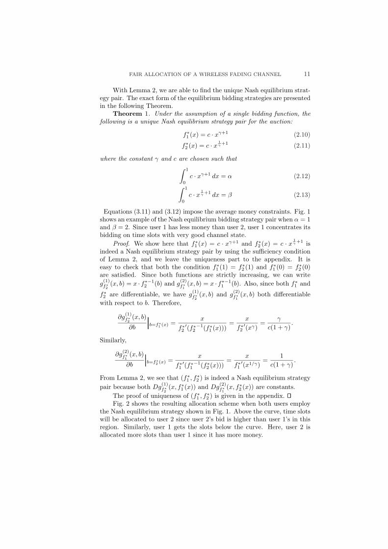
Theorem 1. Under the assumption of a single bidding function, thefollowing is a unique Nash equilibrium strategy pair for the auction:

f∗1 (x) = c · xγ+1 (2.10)

f∗2 (x) = c · x 1γ +1 (2.11)

where the constant γ and c are chosen such that∫ 1

0

c · xγ+1 dx = α (2.12)∫ 1

0

c · x 1γ +1 dx = β (2.13)

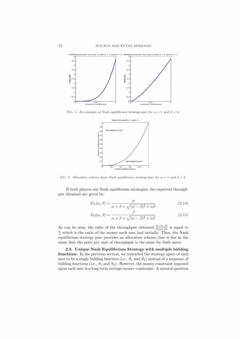
Equations (3.11) and (3.12) impose the average money constraints. Fig. 1shows an example of the Nash equilibrium bidding strategy pair when α = 1and β = 2. Since user 1 has less money than user 2, user 1 concentrates itsbidding on time slots with very good channel state.

Proof. We show here that f∗1 (x) = c · xγ+1 and f∗2 (x) = c · x 1γ +1 is

indeed a Nash equilibrium strategy pair by using the sufficiency conditionof Lemma 2, and we leave the uniqueness part to the appendix. It iseasy to check that both the condition f∗1 (1) = f∗2 (1) and f∗1 (0) = f∗2 (0)are satisfied. Since both functions are strictly increasing, we can writeg(1)f∗2

(x, b) = x · f∗−12 (b) and g

(2)f∗1

(x, b) = x · f∗−11 (b). Also, since both f∗1 and

f∗2 are differentiable, we have g(1)f∗2

(x, b) and g(2)f∗1

(x, b) both differentiablewith respect to b. Therefore,

∂g(1)f∗2

(x, b)

∂b

∣∣∣∣∣∣∣∣∣b=f∗1 (x) =

x

f∗2′(f∗2

−1(f∗1 (x)))=

x

f∗2′(xγ)

=γ

c(1 + γ).

Similarly,

∂g(2)f∗1

(x, b)

∂b

∣∣∣∣∣∣∣∣∣b=f∗2 (x) =

x

f∗1′(f∗1

−1(f∗2 (x)))=

x

f∗1′(x1/γ)

=1

c(1 + γ).

From Lemma 2, we see that (f∗1 , f∗2 ) is indeed a Nash equilibrium strategypair because both Dg

(1)f∗2

(x, f∗1 (x)) and Dg(2)f∗1

(x, f∗2 (x)) are constants.The proof of uniqueness of (f∗1 , f∗2 ) is given in the appendix.Fig. 2 shows the resulting allocation scheme when both users employ

the Nash equilibrium strategy shown in Fig. 1. Above the curve, time slotswill be allocated to user 2 since user 2’s bid is higher than user 1’s in thisregion. Similarly, user 1 gets the slots below the curve. Here, user 2 isallocated more slots than user 1 since it has more money.


0 0.5 10

0.5

1

1.5

2

2.5

3

3.5

4

4.5

5Bidding function for user 1 with α = 1 and β = 2

channel coefficient

mone

y (bid

)

0 0.5 10

0.5

1

1.5

2

2.5

3

3.5

4

4.5

5Bidding function for user 2 with α = 1 and β = 2

channel coefficient

mone

y (bid

)

Fig. 1. An example of Nash equilibrium strategy pair for α = 1 and β = 2.

0 0.2 0.4 0.6 0.8 10

0.1

0.2

0.3

0.4

0.5

0.6

0.7

0.8

0.9

1Result of the bid with α = 1 and β = 2

channel coefficient of user 1

channel coeffic

ient of user

2

slots assigned to user 2

slots assigned to user 1

Fig. 2. Allocation scheme from Nash equilibrium strategy pair for α = 1 and β = 2.

If both players use Nash equilibrium strategies, the expected through-put obtained are given by:

G1(α, β) =α

α + β +√

(α− β)2 + αβ(2.14)

G2(α, β) =β

α + β +√

(α− β)2 + αβ(2.15)

As can be seen, the ratio of the throughput obtained G1(α,β)G2(α,β) is equal to

αβ which is the ratio of the money each user had initially. Thus, the Nashequilibrium strategy pair provides an allocation scheme that is fair in thesense that the price per unit of throughput is the same for both users.

2.3. Unique Nash Equilibrium Strategy with multiple biddingfunctions. In the previous section, we restricted the strategy space of eachuser to be a single bidding function (i.e., S1 and S2) instead of a sequence ofbidding functions (i.e., S1 and S2). However, the money constraint imposedupon each user is a long term average money constraint. A natural question


to ask is the following: Is it profitable for an individual user to change itsbidding functions over time while satisfying the long term average moneyconstraint? Therefore, in this section, we allow the users to use a strategywithin a broader class of strategy space, S1 and S2, and explore whetherthere is an incentive for a user to do so (i.e., whether there exists a Nashequilibrium strategy so that it can increase its throughput).

To choose a strategy (i.e., a sequence of bidding functions) from thestrategy space S1 or S2, a user encounters two problems. First, it mustdecide how to allocate its money among these n bidding functions so thatthe average money constraint is still satisfied. Second, once the moneyallocated to the ith bidding function is specified, a user has to choose abidding function for the ith slot. The second problem is already solvedin the previous section (see Theorem 1). In this section, we will focuson the first problem that a user encounters, specifically, the problem ofhow to allocate money between the bidding functions while satisfying thefollowing condition: The total expected amount of money for the sequenceof n bidding functions is n · α for user 1 and n · β for user 2.

More precisely, the strategy space or possible actions that can be takenby users are the following:

S1 = {α1, · · · , αn | α1 + · · ·+ αn = n · α}S2 = {β1, · · · , βn | β1 + · · ·+ βn = n · β}

The objective of each user is still to maximize its own throughput. Whenuser 1 and user 2 allocate αi and βi for their ith bidding function whichis given in Theorem 1, the payoff functions are G1(αi, βi) for user 1 andG2(αi, βi) for user 2.

The following lemma gives us a Nash equilibrium strategy pair for theauction game described in this section.

Lemma 3. Given that user 2’s strategy is to allocate its money evenlyamong its bidding functions (i.e., βi = β, i = 1 · · ·n), user 1’s best responseis to allocate its money evenly as well (i.e., αi = α, i = 1 · · ·n); and viceversa. Therefore, a Nash equilibrium strategy pair for this auction is forboth users to allocate their money evenly.

Proof. Without loss of generality, we consider the case that n = 2where each user’s strategy can consist of two different bidding functions.Suppose that user 2 allocates β for both bidding functions f

(1)2 and f

(2)2 ,

and user 1 allocates α1 for bidding function f(1)1 and α2 for bidding function

f(2)1 where α1+α2 = 2α and α1 6= α2. We now show that the throughput for

user 1, G1(α1, β) + G1(α2, β), is maximized when α1 = α2 = α. Considerthe function G1(α1, β) with β fixed. The equation

G1(α1, β) =α1

α1 + β +√

(α1 − β)2 + α1β


becomes

F (t) =t

1 + t +√

(1− t)2 + t

where t = α1β . F (t) is concave for t ≥ 0. Thus, we have G1(α1, β) +

G1(α2, β) maximized when α1 = α2 = α.We have already obtained a Nash equilibrium strategy pair from the

above Lemma. The following theorem states that this Nash equilibriumstrategy pair is in fact unique within the strategy space considered.

Theorem 2. For the auction in this section, a unique Nash equilib-rium strategy for both users is to allocate their money evenly among thebidding functions.

Proof. The complete proof is in the Appendix.In this section, users are given more freedom in choosing their strate-

gies (i.e., they can choose n different bidding functions). However, as The-orem 2 shows, the unique Nash equilibrium strategy pair is for each user touse a single bidding function from its strategy space. Thus, the throughputresult obtained in this broader strategy space-S1 and S2–is the same as thethroughput result from previous section. Therefore, there is no incentivefor a user to use different bidding functions.

2.4. Comparison with Other Allocation Schemes. To this end,we have a unique Nash equilibrium strategy pair and the resulting through-put when both players choose to use the Nash equilibrium strategy. In-evitably, due to the fairness constraint, total system throughput will de-crease as compared to the maximum throughput attainable without anyfairness constraint. Hence we would like to compare the total throughputof the Nash equilibrium strategy to that of an unconstrained strategy. Weaddress this question by first considering an allocation scheme that maxi-mizes total throughput subject to no constraint. Then, we investigate thethroughput of another centralized allocation scheme that maximize the to-tal throughput subject to the constraint that the resulting throughput ofindividual user is kept at certain ratio.

2.4.1. Maximizing Throughput with No Constraint. To max-imize throughput without any constraints, the transmitter sends data tothe user with a better channel state during each time slot. Then the ex-pected throughput is E[max{X1, X2}]. Since X1 and X2 are independentuniformly distributed in [0, 1], we have E[max{X1, X2}] = 2

3 . Using theNash equilibrium playing strategy, the total expected system throughput,G1(α, β) + G2(α, β), is 1

2 in the worst case (i.e., one users gets all of thetime slots while the other user is starving). Thus, the channel allocationscheme proposed in this paper can achieve at least 75 percent of the maxi-mum attainable throughput. This gives us a lower bound of the throughputperformance of the allocation scheme derived from the Nash equilibriumpair.


2.4.2. Maximizing Throughput with A Constant ThroughputRatio Constraint. Now, we investigate an allocation scheme with a fair-ness constraint that requires the resulting throughput of the users to bekept at a constant ratio. Specifically, let G1 and G2 denote the expectedthroughput for user 1 and user 2 respectively. We have the following opti-mization problem:

max G1 + G2 subj.G1

G2= a (2.16)

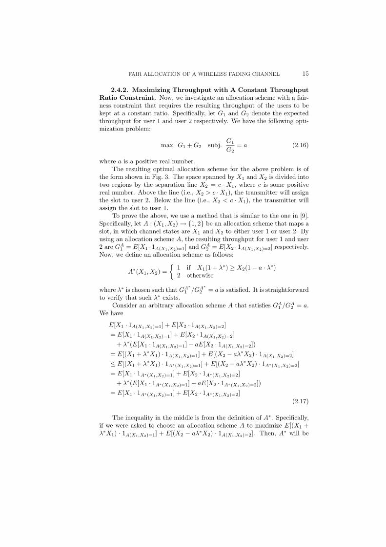
where a is a positive real number.The resulting optimal allocation scheme for the above problem is of

the form shown in Fig. 3. The space spanned by X1 and X2 is divided intotwo regions by the separation line X2 = c · X1, where c is some positivereal number. Above the line (i.e., X2 > c ·X1), the transmitter will assignthe slot to user 2. Below the line (i.e., X2 < c · X1), the transmitter willassign the slot to user 1.

To prove the above, we use a method that is similar to the one in [9].Specifically, let A : (X1, X2) → {1, 2} be an allocation scheme that maps aslot, in which channel states are X1 and X2 to either user 1 or user 2. Byusing an allocation scheme A, the resulting throughput for user 1 and user2 are GA

1 = E[X1 ·1A(X1,X2)=1] and GA2 = E[X2 ·1A(X1,X2)=2] respectively.

Now, we define an allocation scheme as follows:

A∗(X1, X2) ={

1 if X1(1 + λ∗) ≥ X2(1− a · λ∗)2 otherwise

where λ∗ is chosen such that GA∗1 /GA∗

2 = a is satisfied. It is straightforwardto verify that such λ∗ exists.

Consider an arbitrary allocation scheme A that satisfies GA1 /GA

2 = a.We have

E[X1 · 1A(X1,X2)=1] + E[X2 · 1A(X1,X2)=2]= E[X1 · 1A(X1,X2)=1] + E[X2 · 1A(X1,X2)=2]

+ λ∗(E[X1 · 1A(X1,X2)=1]− aE[X2 · 1A(X1,X2)=2])= E[(X1 + λ∗X1) · 1A(X1,X2)=1] + E[(X2 − aλ∗X2) · 1A(X1,X2)=2]≤ E[(X1 + λ∗X1) · 1A∗(X1,X2)=1] + E[(X2 − aλ∗X2) · 1A∗(X1,X2)=2]= E[X1 · 1A∗(X1,X2)=1] + E[X2 · 1A∗(X1,X2)=2]

+ λ∗(E[X1 · 1A∗(X1,X2)=1]− aE[X2 · 1A∗(X1,X2)=2])= E[X1 · 1A∗(X1,X2)=1] + E[X2 · 1A∗(X1,X2)=2]

(2.17)

The inequality in the middle is from the definition of A∗. Specifically,if we were asked to choose an allocation scheme A to maximize E[(X1 +λ∗X1) · 1A(X1,X2)=1] + E[(X2 − aλ∗X2) · 1A(X1,X2)=2]. Then, A∗ will be


1X2X2X

1X

= c

0 1 user 1

user 2

1

Fig. 3. The optimal allocation scheme to achieve constant throughput ratio fairness.

an optimal scheme from its definition. Thus, we are able to show thatA∗(X1, X2) is an optimal solution to the optimization problem in (2.16).

To find the slope c in Fig.3, we first write the throughput for eachuser:

GA∗1 =

∫ 1

0

∫ cx1

0

x1 dx1 dx2 =13c (2.18)

and

GA∗2 =

∫ c

0

∫ 1c x2

0

x2 dx1dx2 +∫ 1

c

x2 dx2 =12− 1

6c2 (2.19)

Since GA1 /GA

2 = a, we get c = −1+√

1+3a2

a .Using the Nash equilibrium strategy pair, the ratio of the resulting

throughput pair G1(α,β)G2(α,β) is the same as the ratio of money individual user

possess (αβ ). For the optimization problem described in (2.16), by setting

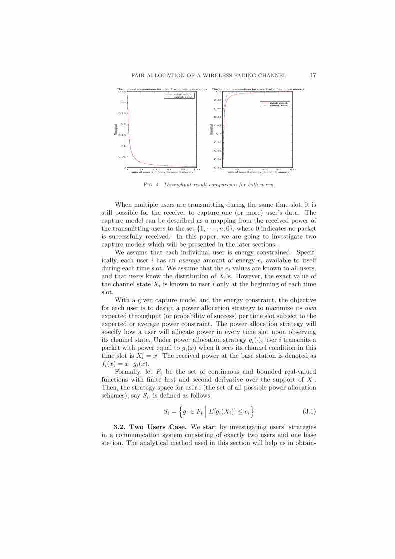
a = α/β, we compare the resulting throughput with the throughput ob-tained when both users employ the Nash equilibrium strategy. Fig. ??and Fig. ?? show the comparison. For both users, the Nash equilibriumthroughput result is very close to the throughput obtained by solving theconstrained optimization problem (within 97 percent to be precise).

3. Uplink Transmission.

3.1. Uplink Problem Formulation. The uplink communication en-vironment that we consider here consists of multiple users who are sendingdata to a single base station or satellite over multiple fading channels. Weassume that each user always has data to be sent to the base station. Timeis assumed to be discrete, and the channel state for a given user changesaccording to a known probabilistic model independently over time. Thechannels between the users and the base station are assumed to be inde-pendent of each other. Let Xi be a random variable denoting the channelstate for the channel between user i and the base station.


0 20 40 60 80 1000

0.05

0.1

0.15

0.2

0.25

0.3

0.35Throughput comparison for user 1 who has less money

ratio of user 2 money to user 1 money

Throu

ghpu

t

nash equil.const. ratio

0 20 40 60 80 1000.32

0.34

0.36

0.38

0.4

0.42

0.44

0.46

0.48

0.5Throughput comparison for user 2 who has more money

ratio of user 2 money to user 1 money

Throu

ghpu

t

nash equil.const. ratio

Fig. 4. Throughput result comparison for both users.

When multiple users are transmitting during the same time slot, it isstill possible for the receiver to capture one (or more) user’s data. Thecapture model can be described as a mapping from the received power ofthe transmitting users to the set {1, · · · , n, 0}, where 0 indicates no packetis successfully received. In this paper, we are going to investigate twocapture models which will be presented in the later sections.

We assume that each individual user is energy constrained. Specif-ically, each user i has an average amount of energy ei available to itselfduring each time slot. We assume that the ei values are known to all users,and that users know the distribution of Xi’s. However, the exact value ofthe channel state Xi is known to user i only at the beginning of each timeslot.

With a given capture model and the energy constraint, the objectivefor each user is to design a power allocation strategy to maximize its ownexpected throughput (or probability of success) per time slot subject to theexpected or average power constraint. The power allocation strategy willspecify how a user will allocate power in every time slot upon observingits channel state. Under power allocation strategy gi(·), user i transmits apacket with power equal to gi(x) when it sees its channel condition in thistime slot is Xi = x. The received power at the base station is denoted asfi(x) = x · gi(x).

Formally, let Fi be the set of continuous and bounded real-valuedfunctions with finite first and second derivative over the support of Xi.Then, the strategy space for user i (the set of all possible power allocationschemes), say Si, is defined as follows:

Si ={

gi ∈ Fi

∣∣∣ E[gi(Xi)] ≤ ei

}(3.1)

3.2. Two Users Case. We start by investigating users’ strategiesin a communication system consisting of exactly two users and one basestation. The analytical method used in this section will help us in obtain-


ing equilibrium power allocation scheme in the multiple users case. Webegin our analysis with the assumption that channel state Xi is uniformlydistributed over [0, 1] for all i. The Nash equilibrium power allocation strat-egy with general channel state distribution is presented in the subsequentsection.

Suppose user 1 and user 2 choose their power allocation strategies tobe g1 and g2 respectively. Given a time slot with channel state realization(x1, x2), user 1 and user 2 will transmit their packets using power levelsg1(x1) and g2(x2) respectively. The corresponding received power at thebase station are f1(x1) = x1 · g1(x1) and f2(x2) = x2 · g2(x2). As in[12] and [13], the capture model used in this section is the following: if[x1 ·g1(x1)]/[x2 ·g2(x2)] ≥ K where K ≥ 1, user 1’s packet will be captured.Likewise, user 2’s packet will be captured if [x2 · g2(x2)]/[x1 · g1(x1)] ≥ K.Thus, given a power allocation strategy pair (g1, g2), where g1 ∈ S1 andg2 ∈ S2, the expected throughput for user 1 is defined as the following:

G1(e1, e2) = EX1,X2 [1f1(X1)≥K·f2(X2)] (3.2)

where

1f1(X1)≥f2(X2) ={

1 if f1(X1) ≥ K · f2(X2)0 otherwise

Similarly, the throughput function for user 2:

G2(e1, e2) = EX1,X2 [1f2(X2)>K·f1(X1)] (3.3)

3.2.1. Nash equilibrium strategy. In this part, we present a Nashequilibrium power allocation strategy pair (g∗1 , g∗2). The derivation of theNash equilibrium is similar to the derivation of the Nash equilibrium in theall-pay auction part. We consider here the case where both users choosetheir strategies from the strategy space S1 and S2 and the value of e1 ande2 are known to both users.

To get the Nash equilibrium strategy pair, we first argue that at equi-librium the received power function f∗i (xi) must be strictly increasing inxi.

Lemma 4. Given a Nash equilibrium power allocation strategy pair(g∗1 , g∗2) and its corresponding received power function (f∗1 , f∗2 ), the receivedpower function f∗1 (x1) must be strictly increasing in x1. Similarly, f∗2 (x2)must be strictly increasing in x2.

Proof. For an arbitrary received power function f which is not strictlyincreasing, we can always find another received power function that willresult in a larger throughput gain. To see this, consider time slots withchannel state in the small intervals (a − δ, a + δ) and (b − δ, b + δ) wherea < b. When δ is small, the received power function is close to f(a) for timeslots in the interval (a− δ, a + δ). Likewise, the received power function isclose to f(b) for time slots in the interval (b− δ, b + δ).


For received power function f such that f(a) = a·g(a) > f(b) = b·g(b)for some a < b. The total amount of transmission power used in time slotswith channel state in the two intervals is given by:

[g(a) + g(b)]2δ = [f(a)

a+

f(b)b

]2δ.

Now, if user 1 employs a new power allocation strategy g such that g(b) =f(a)

b and g(a) = f(b)a , user 1 will achieve the same expected throughput

as before. However, the amount of power used [g(b) + g(a)]2δ is less than[g(a) + g(b)]2δ, and the extra power can be used to get higher throughput.Hence, both equilibrium received power function f∗1 (x1) and f∗2 (x2) mustbe strictly increasing in x1 and x2 respectively.

With one user’s power allocation strategy, say g2, fixed, we now seekthe optimal power allocation scheme for user 1. From Lemma 4, we seethat the inverse of f1 and f2 are well defined. With user 2’s strategy g2

fixed, let u(1)g2 : (x1, b) → R denote user 1’s expected throughput of a slot

conditioning on the following events:• User 1’s channel state is X1 = x1.• User 1’s allocated power is b.

For convenience, we will drop the term g2 in the expression u(1)g2 (x1, b), and

simply write it as u1(x1, b). Specifically, we can the write the equation:

u1(x1, b) = P (f2(X2) ·K ≤ x1 · b) (3.4)

where P (f2(X2) ·K ≤ x1 ·b) is the probability that user 1’s packet gets cap-tured in a time slot. Consequently, using a strategy g1, user 1’s throughputis given by:

G1(e1, e2) =∫ 1

0

u1(x1, g1(x1)) · pX1(x1) dx1 =∫ 1

0

u1(x1, g1(x1)) dx1

(3.5)

where the last equality results from the uniform distribution assumption.With user 1’s strategy g1 fixed, similar terms for user 2 can be defined.

u2(x2, b) = u(2)g1

(x2, b) = P (f1(X1) ·K ≤ x2 · b)Then, user 2’s throughput is given by:

G2(e1, e2) =∫ 1

0

u2(x2, g2(x2)) · pX2(x2) dx2 =∫ 1

0

u2(x2, g2(x2)) dx2

(3.6)

Due to the uniformly distributed channel state, P (f2(X2) ·K ≤ x1 · b)is given by

P (f2(X2) ·K ≤ x1 · b) = P (X2 ≤ f−12 (

1K

x1 · b)) = f−12 (

1K

x1 · b)


where f−12 is well defined. Thus, we can rewrite Eq. (3.4) as

u1(x1, b) = f−12 (

1K

x1 · b).

Hence we have,

G1(e1, e2) =∫ 1

0

f−12 (

1K

x1 · g1(x1)) dx1 (3.7)

G2(e1, e2) =∫ 1

0

f−11 (

1K

x2 · g2(x2)) dx2 (3.8)

We begin our analysis of the Nash equilibrium strategy pair by firstconsidering the power allocation on the boundary points 0 and 1. Fora pair of power allocation functions (g∗1 , g∗2) to be a Nash equilibrium, itis straightforward to see that g∗1(0) = g∗2(0) = 0 since it does not makesense to allocate power for a slot with zero channel state. Likewise, wemust have g∗1(1) ≤ K · g∗2(1) and g∗2(1) ≤ K · g∗1(1) since allocating powerg1(1) = Kg2(1) or g1(1) = Kg2(1) + ε, where ε > 0, will result in the samethroughput for user 1. We call these properties the boundary conditions ofa Nash equilibrium strategy pair.

With the boundary conditions satisfied, the following lemma gives anecessary and sufficient condition for a pair of power allocation strategiesto be a Nash equilibrium strategy pair. For convenience, we denote themarginal gain for user 1 when X1 = x1 and the allocated power b = b∗ as

∂u1(x1, b)∂b

|||b=b∗4= Du1(x1, b

∗).

Lemma 5. Given a power allocation strategy pair (g∗1 , g∗2) that satisfiesthe boundary conditions, (g∗1 , g∗2) is a Nash equilibrium strategy pair if andonly if Du1(x1, g

∗1(x1)) = c1 and Du2(x2, g

∗2(x2)) = c2, for some constants

c1 and c2, for all x1 ∈ [0, 1] and all x2 ∈ [0, 1].Note that the above lemma does not depend on the assumption of

the uniformly distributed channel state. Thus, it is quite general and willbe used in the subsequent section where channel states are not uniformlydistributed. The proof is similar to the proof of Lemma 2.

With Lemma 5, we are able to find the Nash equilibrium strategy pair.The exact form of the equilibrium power allocation strategies are presentedin the following Theorem.

Theorem 3. Given the average power constraint e1 and e2, the Nashequilibrium power allocation strategy pair has the following form:

g∗1(x) = c1 · xγ (3.9)

g∗2(x) = c2 · x1γ (3.10)


where the constants c1, c2 and γ are chosen such that

∫ 1

0

c1 · xγ dx = e1 (3.11)∫ 1

0

c2 · x1γ dx = e2 (3.12)

Equations (3.11) and (3.12) impose the average power constraints.The proof of the above theorem is similar to the proof of Theorem 1.

From the above theorem, we see that equations (3.9) and (3.10) specifythe Nash equilibrium power allocation strategy pair. Since there are twoequations with three unknowns, the resulting Nash equilibrium may not beunique in general. However, if a packet with stronger received power canalways be captured (i.e., K = 1), the Nash equilibrium power allocationstrategy is unique.

Corollary 1. For K = 1, the unique Nash equilibrium power alloca-tion pair has the following form:

g∗1(x) = c · xγ , g∗2(x) = c · x 1γ (3.13)

where the constants c and γ are chosen such that the average power con-straints are satisfied.

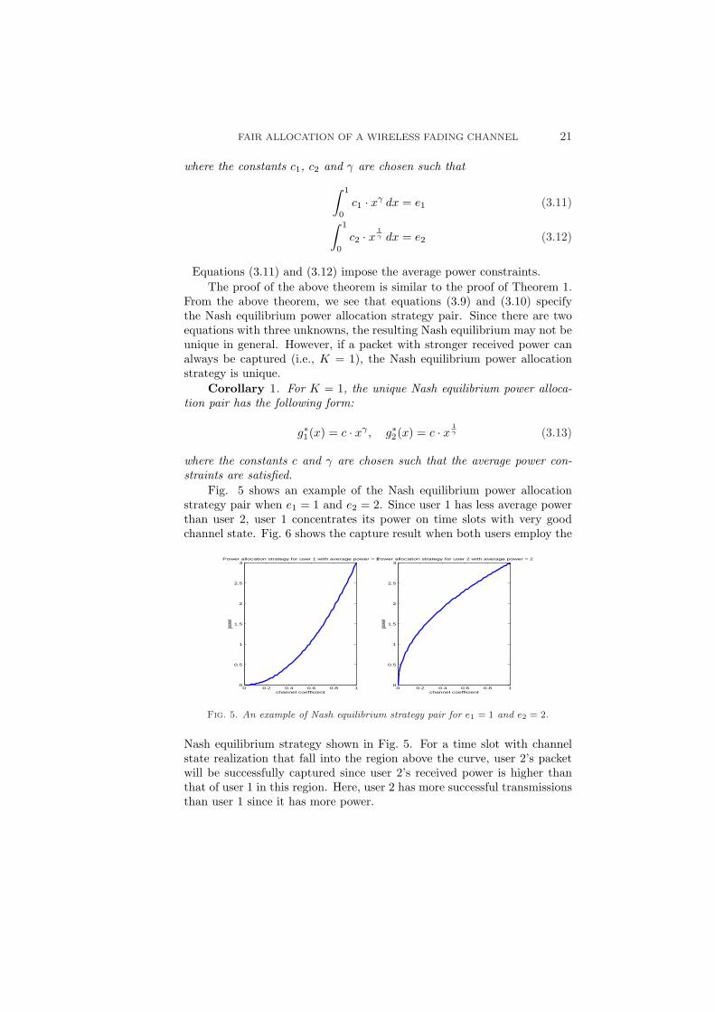
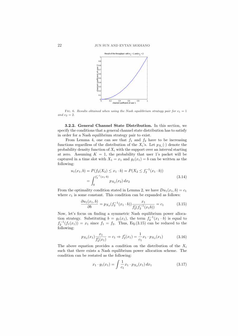
Fig. 5 shows an example of the Nash equilibrium power allocationstrategy pair when e1 = 1 and e2 = 2. Since user 1 has less average powerthan user 2, user 1 concentrates its power on time slots with very goodchannel state. Fig. 6 shows the capture result when both users employ the

0 0.2 0.4 0.6 0.8 10

0.5

1

1.5

2

2.5

3Power allocation strategy for user 1 with average power = 1

channel coefficient

powe

r

0 0.2 0.4 0.6 0.8 10

0.5

1

1.5

2

2.5

3Power allocation strategy for user 2 with average power = 2

channel coefficient

powe

r

Fig. 5. An example of Nash equilibrium strategy pair for e1 = 1 and e2 = 2.

Nash equilibrium strategy shown in Fig. 5. For a time slot with channelstate realization that fall into the region above the curve, user 2’s packetwill be successfully captured since user 2’s received power is higher thanthat of user 1 in this region. Here, user 2 has more successful transmissionsthan user 1 since it has more power.


0 0.2 0.4 0.6 0.8 10

0.1

0.2

0.3

0.4

0.5

0.6

0.7

0.8

0.9

1

Result of the throughput with e1 = 1 and e

2 = 2

channel coefficient of user 1

ch

an

ne

l co

eff

icie

nt

of

use

r 2

Fig. 6. Results obtained when using the Nash equilibrium strategy pair for e1 = 1and e2 = 2.

3.2.2. General Channel State Distribution. In this section, wespecify the conditions that a general channel state distribution has to satisfyin order for a Nash equilibrium strategy pair to exist.

From Lemma 4, one can see that f1 and f2 have to be increasingfunctions regardless of the distribution of the Xi’s. Let pXi(·) denote theprobability density function of Xi with the support over an interval startingat zero. Assuming K = 1, the probability that user 1’s packet will becaptured in a time slot with X1 = x1 and g1(x1) = b can be written as thefollowing:

u1(x1, b) = P (f2(X2) ≤ x1 · b) = P (X2 ≤ f−12 (x1 · b))

=∫ f−1

2 (x1·b)

0

pX2(x2) dx2

(3.14)

From the optimality condition stated in Lemma 2, we have Du1(x1, b) = c1

where c1 is some constant. This condition can be expanded as follows:

∂u1(x1, b)∂b

= pX2(f−12 (x1 · b)) x1

f ′2(f−12 (x1b))

= c1 (3.15)

Now, let’s focus on finding a symmetric Nash equilibrium power alloca-tion strategy. Substituting b = g1(x1), the term f−1

2 (x1 · b) is equal tof−12 (f1(x1)) = x1 since f1 = f2. Thus, Eq.(3.15) can be reduced to the

following:

pX2(x1)x1

f ′2(x1)= c1 ⇒ f ′2(x1) =

1c1

x1 · pX2(x1) (3.16)

The above equation provides a condition on the distribution of the Xi

such that there exists a Nash equilibrium power allocation scheme. Thecondition can be restated as the following:

x1 · g1(x1) =∫

1c1

x1 · pX2(x1) dx1 (3.17)


From the above condition, for example, we see that if pX2(·) is a strictly in-creasing polynomial, there exist a Nash equilibrium power allocation strat-egy.

3.3. Multiple Users Equilibrium Strategies. In this section, weexplore the Nash equilibrium power allocation strategies when n users arecompeting to access the single base station. User i’s power allocationfunction is denoted as gi(·). Given a time slot with channel state real-ization ~x = (x1, · · · , xn), the transmitting power for each user is gi(xi).The corresponding received power at the base station is again denoted asfi(xi) = xi ·gi(xi). The new capture rule used in this section is given as thefollowing: a packet from user 1 will be successfully received if the followingholds:

f1(x1) ≥ (1 + ∆) max(f2(x2), · · · , fn(xn))

Similar capture model can be found in [15] (i.e., protocol model). Thequantity ∆ models situations where a guard zone is specified to preventinterference. Note also that the capture rule used in the two users’ casecan be viewed as a special case the above capture rule.

We start with each user facing the same average power constraint (i.e.,e1 = e2 = · · · = en). Since users are identical, it is reasonable to seek asymmetric Nash equilibrium power allocation strategy. Specifically, the setof strategies (g1 = g, · · · , gn = g) is said to be a symmetric Nash equi-librium strategies if gi = g is the best power allocation strategy for useri when all other users are also employing the power allocation strategyg. For a power allocation function g to be a symmetric Nash equilibriumstrategy, f(x) = xg(x) must be a strictly increasing function using a sim-ilar argument as in the two users case. The following theorem shows theexistence and the form of a symmetric Nash equilibrium power allocationstrategy.

Theorem 4. Given that each user has the same average power con-straint, there exists a symmetric Nash equilibrium power allocation strategywith the following form:

gi(xi) = c · xn−1i ∀ i ∈ {1, · · · , n} (3.18)

where c is chosen such that the average power constraint is satisfied.Proof. The complete proof is given in the Appendix.With the symmetric Nash equilibrium power allocation strategy given

in Eq.(3.18), the expected throughput for each user is given by:

P (f(X1) ≥ (1 + ∆) max(f(X2), · · · , f(Xn)))= P (Xn

1 ≥ (1 + ∆) max(Xn2 , · · · , Xn

n ))

= P (X1 ≥ (1 + ∆)1n max(X2, · · · , Xn))

(3.19)


To quantify the loss of efficiency due to users’ selfish behavior, we consider asystem where all users implement the same power allocation policy providedby a system designer such that the overall system throughput is maximized.To find such scheme, we solve the following optimization problem as in thetwo users’ case:

maxv∈S1

P (X1v(X1) ≥ (1 + ∆) ·max(X2v(X2), · · · , Xnv(Xn))

By symmetry, we have the following upper bound for the above probability:

P (X1v(X1) ≥ (1 + ∆) ·max(X2v(X2), · · · , Xnv(Xn)) <1n

As in the two users’ case, we consider a series of functions, vm(x) = xm form ≥ 1. As m →∞, we have

P (Xm+11 ≥ (1 + ∆) ·max(Xm+1

2 , · · · , Xm+1n ))

= P (X1 ≥ (1 + ∆)1

m+1 max(X2, · · · , Xn)) → 1n

Thus, there indeed exists a power allocation scheme that will achieve themaximum possible throughput. In other words, it is possible to have apacket successfully captured in every time slot. Now, when users behaveselfishly, the expected throughput for each user is given as follows fromEq.(3.19):

P (X1 ≥ (1 + ∆)1n max(X2, · · · , Xn)) (3.20)

As n increases, the above equation goes to 1/n which is the maximumattainable throughput. Therefore, as the number of users becomes large,the symmetric Nash equilibrium power allocation scheme is optimal in thesense that the throughput obtained approaches the maximum attainablethroughput.

For the special case where ∆ = 0, the capture rule becomes that theuser with the largest received power get captured. With this simple rule, aNash equilibrium strategy can be derived with general channel state distri-bution (i.e., Xi has probability density function pXi(·)). From Eq.(4.23),we have

pZ(f−1(x1 · b)) x1

f ′(f−1(x1 · b)) = c

f ′(x1) =1cx1pZ(x1)

(3.21)

where

pZ(z) = (n− 1)pX1(z)[∫ z

0

pX1(x) dx]n−2.


Hence, we can write the received power function as the following:

f(x) =1c

∫xpZ(x) dx

From the above equation, one can get the optimal power allocation functionby using g(x) = f(x)

x .

4. Conclusion. We apply an auction algorithm to the problem of fairallocation of a wireless fading channel. Using the all-pay auction mecha-nism, we are able to obtain a unique Nash equilibrium strategy. Our strat-egy allocated bandwidth to the users in accordance with the amount ofmoney that they possess. Hence, this scheme can be viewed as a mecha-nism for providing quality of service (QoS) differentiation; whereby usersare given fictitious money that they can use to bid for the channel. By al-locating users different amounts of money, the resulting QoS differentiationcan be achieved.

We also show that the Nash equilibrium strategy of this auction leadsto an allocation at which total throughput is no worse than 3/4 the maxi-mum possible throughput when fairness constraints are not imposed (i.e.,slots are allocated to the user with the better channel). In this paper, wefocused on finding a Nash equilibrium strategy when both channels areuniformly distributed. However, as we mentioned earlier, our analysis canbe extended to channel state with general distribution. An interesting ex-tension could be to find the exact form of a Nash equilibrium with generalchannel state distribution.

In the uplink communication scenario, we consider a communicationsystem with multiple users competing, in a non-cooperative manner, for theaccess of a single satellite, or base station. With a specified capture ruleand an average power constraint, users opportunistically adjust their trans-mission power based on their channel state to maximize their throughput.A Nash equilibrium power allocation strategy is characterized, and the re-sulting throughput efficiency loss, due to selfish behavior, is quantified. Asthe number of users increases, the Nash equilibrium power allocation strat-egy approaches the optimal power allocation strategy that can be achievedin a cooperative environment.

Appendix.

Proof of Lemmma 2. Proof: We first show that if (f∗1 , f∗2 ) is a Nashequilibrium strategy pair, Dg

(1)f∗2

(x1, f∗1 (x1)) and Dg

(2)f∗1

(x2, f∗2 (x2)) must be

constants for all x1 ∈ [0, 1] and x2 ∈ [0, 1]. From user 1’s perspectivewith f∗2 fixed, consider a small variation of the function f∗1 . Specifically, letfδ = f∗1 +δ(f−f∗1 ) where f is an arbitrary function in S1. Since both f andf∗1 are in S1, they are both bounded (i.e., |f(x1)| ≤ B and |f∗1 (x1)| ≤ Bfor all x1 ∈ [0, 1]). Therefore, we have |fδ(x1) − f∗1 (x1)| ≤ 2Bδ for all


x1 ∈ [0, 1]. Using the Lagrange’s form of Taylor’s theorem, we get for anyx1 ∈ [0, 1], there exists a real number c[x1] ∈ [f∗1 (x1), fδ(x1)] such that

g(1)f∗2

(x1, fδ(x1)) = g(1)f∗2

(x1, f∗1 (x1))

+ δ(f(x1)− f∗1 (x1))∂g

(1)f∗2

(x1, b)

∂b

∣∣∣∣∣∣∣∣∣b=f∗1 (x1)

+12δ2(f(x1)− f∗1 (x1))2

∂2g(1)f∗2

(x1, b)

∂b2

∣∣∣∣∣∣∣∣∣b=c[x1]

(4.1)

The last term is bounded by K · δ2 for some K since both f and f∗1 arebounded, and g

(1)f∗2

(x1, b) has finite second derivative. Therefore, for smallenough δ, it is negligible comparing with the other terms.

Now we show that if Dg(1)f∗2

(x1, f∗1 (x1)) is not a constant for all x1 ∈

[0, 1], we can find a strategy fδ which gives user 1 a higher throughput thanf∗1 . To do that, we can write the following equations:

∫ 1

0

g(1)f∗2

(x1, fδ(x1)) dx1 −∫ 1

0

g(1)f∗2

(x1, f∗1 (x1)) dx1

= δ

∫ 1

0

(f(x1)− f∗1 (x1))∂g

(1)f∗2

(x1, b)

∂b

∣∣∣∣∣∣∣∣∣b=f∗1 (x1) dx1 + o(δ)

(4.2)

Now, since Dg(1)f∗2

(x1, f∗1 (x1)) is not a constant for all x1 ∈ [0, 1], we can

find a f such that the above equation is positive which implies that there isan incentive for user 1 to use fδ. Hence, (f∗1 , f∗2 ) is not a Nash equilibriumstrategy pair. Similarly, we can show that Dg

(2)f∗1

(x2, f∗2 (x2)) is a constant

for all x2 ∈ [0, 1] if (f∗1 , f∗2 ) is a Nash equilibrium strategy pair.For the converse, consider again Eq.(4.2). Since Dg

(1)f∗2

(x1, f∗1 (x1)) =

∂g(1)f∗2

(x1,b)

∂b

∣∣∣∣∣∣∣∣∣b=f∗1 (x1) equals to a constant c1 for all x1 ∈ [0, 1]. We have

δ

∫ 1

0

(f(x1)− f∗1 (x1))∂g

(1)f∗2

(x1, b)

∂b

∣∣∣∣∣∣∣∣∣b=f∗1 (x1) dx1

= δc1

∫ 1

0

(f(x1)− f∗1 (x1)) dx1 = 0

(4.3)

for all f ∈ S1 (i.e.,∫ 1

0f(x1) dx1 = α). Thus, there is no incentive for user 1

to use strategy f . Therefore, (f∗1 , f∗2 ) is a Nash equilibrium strategy pair.

Proof of Theorem 1 (the Uniqueness ). Consider any Nash equi-librium strategy pair (f1, f2) under the all-pay auction rule. From previousdiscussion, we know that the inverse functions, f−1

2 and f−11 , are well de-

fined. With user 2’s strategy f2 fixed, we have

g(1)f2

(x1, b) = x1 · P (f2(X2) ≤ b) = x1 · f−12 (b)


Similarly, with user1’s strategy f1 fixed, we get

g(2)f1

(x2, b) = x2 · P (f1(X1) ≤ b) = x2 · f−11 (b)

From Lemma 2, we know that Dg(1)f2

(x1, f1(x1)) and Dg(2)f1

(x2, f2(x2)) aretwo constants for all x1 ∈ [0, 1] and x2 ∈ [0, 1] since (f1, f2) is a Nashequilibrium strategy pair.

Now, consider the set of channel state pair (x1, x2) such that f1(x1) =f2(x2) (i.e., two users’ bids are equal). It forms a separation line in spacespan by X1 and X2. Mathematically, this line can be defined as h : [0, 1] →[0, 1] such that x2 = h(x1) = f−1

2 (f1(x1)). By the all-pay auction rule, aslot with channel state (x1, x

′2) will be assigned to user 2 if (x1, x

′2) is

above the line x2 = h(x1) and to user 1 if (x1, x′2) is below the separation

line. Fig.2 shows an example of h(x1). The following lemma shows theuniqueness of h(x1). We then derive the uniqueness of the strategy pair(f1, f2) from the lemma.

Lemma 6. If Dg(1)f2

(x1, f1(x1)) and Dg(2)f1

(x2, f2(x2)) are two con-stants, c1 and c2 respectively, for all x1 ∈ [0, 1] and x2 ∈ [0, 1], thenh(x1) = x

c1/c21 .

Proof. Since Dg(1)f2

(x1, f1(x1)) = c1, from g(1)f2

(x1, b) = x1 · f−12 (b), we

have

Dg(1)f2

(x1, f1(x1)) =∂g

(1)f2

(x1, b)∂b

∣∣∣∣∣∣∣∣∣b=f1(x1) =

x1

f ′2(f−12 (f1(x1)))

= c1

f ′2(h(x1)) =x1

c1(4.4)

Similarly, for user 2, we get

Dg(2)f1

(x2, f2(x2)) =∂g

(2)f1

(x2, b)∂b

∣∣∣∣∣∣∣∣∣b=f2(x2) =

x2

f ′1(f−11 (f2(x2)))

= c2

f ′1(h−1(x2)) =

x2

c2(4.5)

We also know that f1(x1) = f2(h(x1)) and f ′1(x1) = f ′2(h(x1)) ·h′(x1).Thus, we have

f ′1(h−1(x2)) = f ′2(h(h−1(x2))) · h′(h−1(x2))

= f ′2(x2) · h′(x1) = f ′2(h(x1)) · h′(x1)(4.6)

By combining the equations f ′1(h−1(x2)) = x2

c2and f ′1(h

−1(x2)) =f ′2(h(x1)) · h′(x1), we get

x2

c2= f ′2(h(x1)) · h′(x1).


Next we substitute Eq.(4.4) and x2 = h(x1) in the above equation to obtain,

x1 · dh(x1)dx1

=c1

c2h(x1) ⇒ dh(x1)

h(x1)=

c1

c2

dx1

x1

ln |h(x1)| = c1

c2ln |x1|+ c3 ⇒ h(x1) = ec3 · x

c1c21

Combined with fact that h(1) = 1, we get h(x1) = xc1c21 .

Now, we are in a position to derive the exact form of the Nash equilib-rium strategy pair. From the equations f ′1(h

−1(x2)) = x2c2

and x2 = h(x1),

we get f ′1(x1) = h(x1)c2

= xc1c21 /c2. Combined with the condition that

f1(0) = 0, we have f1(x) = 1c1+c2

xc1c2

+1. Following the similar method,

we get f2(x) = 1c1+c2

xc2c1

+1. Let γ = c1c2

and c = 1c1+c2

, the Nash equilib-rium strategy pair for the all-pay auction must have the following form:

f∗1 (x1) = c · xγ+11 , f∗2 (x2) = c · x

1γ +1

1 (4.7)

The constant γ and c are chosen such that equations (3.11) and (3.12)are satisfied. The uniqueness of the above Nash equilibrium strategy comesfrom the fact that there is a unique pair of c and γ that satisfy equations(3.11) and (3.12).

Proof of Theorem 2. Proof. Again, we consider n = 2 case forsimplicity. For α1+α2 = 2α and β1+β2 = 2β, this theorem stated that thepair (α1, β1) and (α2, β2) cannot be in equilibrium if α1 6= α2 and β1 6= β2.We will show this by contradiction. Suppose the pair (α1, β1) and (α2, β2)are in equilibrium for α1 6= α2 and β1 6= β2. That is, for given β1 and β2,α1 and α2 are chosen such that user 1’s throughput G1(α1, β1)+G1(α2, β2)is the maximum. This implies the following:

∂G1(α, β1)∂α

∣∣∣∣∣∣∣∣∣α=α1 =

∂G1(α, β2)∂α

∣∣∣∣∣∣∣∣∣α=α2 . (4.8)

To see this, if ∂G1(α,β1)∂α

∣∣∣∣∣∣∣∣∣α=α1 > ∂G1(α,β2)

∂α

∣∣∣∣∣∣∣∣∣α=α2 , we will have G1(α1+δ, β1)+

G1(α2 − δ, β2) > G1(α1, β1) + G1(α2, β2) by first order expansion, thuscontradicting the statement that G1(α1, β1) + G1(α2, β2) is the maximumthroughput for user 1 for given β1 and β2.

Similarly, for given α1 and α2, if β1 and β2 maximize G2(α1, β1) +G2(α2, β2) then,

∂G2(α1, β)∂β

∣∣∣∣∣∣∣∣∣β=β1 =

∂G2(α2, β)∂β

∣∣∣∣∣∣∣∣∣β=β2 . (4.9)

By taking the derivative of equations (2.14) and (2.15), we get the


following:

∂G1(α, β1)∂α

∣∣∣∣∣∣∣∣∣α=α1 = − β1(−2

√α2

1 − α1β1 + β21 + α1 − 2β1)

2(α1 + β1 +√

α21 − α1β1 + β2

1)2√

α21 − α1β1 + β2

1

(4.10)

∂G2(α1, β)∂β

∣∣∣∣∣∣∣∣∣β=β1 = − α1(−2

√α2

1 − α1β1 + β21 + β1 − 2α1)

2(α1 + β1 +√

α21 − α1β1 + β2

1)2√

α21 − α1β1 + β2

1

(4.11)

Substituting Eq.(4.10) into Eq.(4.8) and Eq.(4.11) into Eq.(4.9), wethen have the following after combining Eq.(4.8) and Eq.(4.9):

β1(−2√

α21 − α1β1 + β2

1 + α1 − 2β1)β2(−2

√α2

2 − α2β2 + β22 + α2 − 2β2)

=α1(−2

√α2

1 − α1β1 + β21 + β1 − 2α1)

α2(−2√

α22 − α2β2 + β2

2 + β2 − 2α2)

(4.12)

To simplify the above equation, we multiply α22

α21

on both sides, and let

γ1 = β1α1

, γ2 = β2α2

. We get

γ1(−2√

1− γ1 + γ21 + 1− 2γ1)

γ2(−2√

1− γ2 + γ22 + 1− 2γ2)

=−2

√1− γ1 + γ2

1 + γ1 − 2−2

√1− γ2 + γ2

2 + γ2 − 2(4.13)

or, after rearranging terms, the following:

γ1(−2√

1− γ1 + γ21 + 1− 2γ1)

−2√

1− γ1 + γ21 + γ1 − 2

=γ2(−2

√1− γ2 + γ2

2 + 1− 2γ2)−2

√1− γ2 + γ2

2 + γ2 − 2(4.14)

We define

f(γ) =γ(−2

√1− γ + γ2 + 1− 2γ)

−2√

1− γ + γ2 + γ − 2.

Then Eq.(4.14) becomes f(γ1) = f(γ2). Now we show that this impliesγ1 = γ2 by observing that

∂f(γ)∂γ

= − (γ + 1)(2√

1− γ + γ2 − 1 + 2γ)√1− γ + γ2(−2

√1− γ + γ2 + γ − 2)

,

and it is easy to check that ∂f∂γ > 0 ∀γ ≥ 0. Now, we have β1

α1= β2

α2. We

further show that α1 = α2 and β1 = β2. Observe that for fixed β1 and β2,


we can write

G1(α, β1) =α

α + β1 +√

(α− β1)2 + αβ1

=αβ1

1 + αβ1

+√

(1− αβ1

)2 + αβ1

, F (α

β1)

(4.15)

where

F (σ) =σ

1 + σ +√

(1− σ)2 + σ.

Thus, we have

∂G1(α, β1)∂α

∣∣∣∣∣∣∣∣∣α=α1 =

1β1

∂F (σ)∂σ

∣∣∣∣∣∣∣∣∣σ=

α1β1

(4.16)

∂G1(α, β2)∂α

∣∣∣∣∣∣∣∣∣α=α2 =

1β2

∂F (σ)∂σ

∣∣∣∣∣∣∣∣∣σ=

α2β2

(4.17)

From Eq.(4.8), we have

1β1

∂F (σ)∂σ

∣∣∣∣∣∣∣∣∣σ=

α1β1

=1β2

∂F (σ)∂σ

∣∣∣∣∣∣∣∣∣σ=

α2β2

(4.18)

It is easy to verify that ∂F (σ)∂σ 6= 0 ∀σ ≥ 0. Therefore, since β1

α1= β2

α2,

the above equation implies that β1 = β2 which contradicts our originalassumption of β1 6= β2. Therefore, the pair (α1, β1) and (α2, β2) cannot bein equilibrium if α1 6= α2 and β1 6= β2.

Proof of Theorem 4. Proof. With all users i 6= 1 using a fixed powerallocation strategy g, we now explore the optimal power allocation strategyfor user 1 which is denoted by g∗1 . Let u

(1)g : (x1, b) → R denote user 1’s

expected throughput during a slot conditioning on the following events:• User 1’s channel state is X1 = x1.• User 1’s allocated power is b.

As before, we will drop the term g in the expression u(1)g (x1, b), and simply

write it as u1(x1, b). Specifically, we can the write the equation:

u1(x1, b) =P ((1 + ∆) max(f2(X2), · · · , fn(Xn)) ≤ x1 · b)=P ((1 + ∆)Y ≤ x1 · b)

where Y = max(f2(X2), · · · , fn(Xn)). Since all users i 6= 1 use the samestrategy g, we have Y = max(f(X2), · · · , f(Xn)) where f(Xi) = Xi · g(Xi)for all i 6= 1. Moreover, since f is strictly increasing, we can write:

Y = max(f(X2), · · · , f(Xn)) = f(max(X2, · · · , Xn))


Denoting Z = max(X2, · · · , Xn), we have the following:

u1(x1, b) = P ((1 + ∆)Y ≤ x1 · b) = P (Z ≤ f−1(1

1 + ∆x1 · b))

=∫ f−1( 1

1+∆ x1·b)

0

pZ(z) dz

(4.19)

where pZ(·) denote the probability density function of the random variableZ. The optimization problem that user 1 faces can be written as thefollowing:

maxG1(e) =∫ 1

0

u1(x1, g1(x1)) · pX1(x1) dx1 =∫ 1

0

u1(x1, g1(x1)) dx1

subj.∫ 1

0

g1(x1) dx1 ≤ e

(4.20)

Writing the Lagrangian function, we have∫ 1

0

u1(x1, g1(x1)) dx1 − λ(∫ 1

0

g1(x1) dx1 − e)

=∫ 1

0

[u1(x1, g1(x1))− λg1(x1)] dx1 + λe

(4.21)

Therefore, for each fixed x1, we want to choose a g1(x1) to maximize theterm u1(x1, g1(x1)) − λg1(x1). For convenience, let b = g1(x1). Then, wehave

maxb

L(b) = maxb

u1(x1, b)− λb = maxb

∫ f−1( 11+∆ x1·b)

0

pZ(z) dz − λb (4.22)

Maximizing L(b) with respect to b yields the first order condition:

∂L(b)∂b

= pZ(f−1(1

1 + ∆x1 · b))

x11+∆

f ′(f−1( 11+∆x1 · b))

− λ = 0 (4.23)

Since Z = max(X2, · · · , Xn) and Xi’s are i.i.d, we have

pZ(z) = (n− 1)zn−2.

Now, consider b = g1(x1) = cxm1 . Since we are seeking a symmetric Nash

equilibrium power allocation strategy, user i 6= 1 will adopt the same strat-egy as user 1. Thus, we have f(x) = x · g(x) = x · cxm = cxm+1. Thesecond term in Eq.(4.23) can be written as the following:

f ′(f−1(1

1 + ∆x1 · b)) = f ′(f−1(

c

1 + ∆x1 · xm

1 ))

= f ′((1

1 + ∆x1 · xm

1 )1

m+1 ) = c(m + 1)(1

1 + ∆)

mm+1 xm

1

(4.24)


Similarly,

pZ(f−1(1

1 + ∆x1 · b)) = pZ((

11 + ∆

)1

m+1 x1) = (n− 1)(1

1 + ∆)

n−2m+1 xn−2

1

(4.25)

Eq.(4.23) can be re-written in the following form:

(n− 1)(1

1 + ∆)

n−2m+1 xn−2

1

x11+∆

c(m + 1)( 11+∆ )

mm+1 xm

1

− λ = 0 (4.26)

Since the above equality has to hold for all x1 ∈ [0, 1], the following mustbe true

xn−21 · x1 · x−m

1 = 1

Thus, we have m = n− 1 and gi(x) = cxn−1 for all i = 1, · · · , n.

REFERENCES

[1] A. Fu, E. Modiano, and J. Tsitsiklis, “Optimal energy allocation for delay-constrained data transmission over a time-varying channel,” IEEE INFOCOM2003, San Francisco, CA, April 2003.

[2] P. Marbach and R. Berry, “Downlink resource allocation and pricing for wirelessnetworks,” IEEE INFOCOM 2002, New York, NY, June 2002.

[3] P. Marbach, “Priority service and max-min fairness,” IEEE INFOCOM 2002, NewYork, NY, June 2002.

[4] P. Viswanath, D. Tse, and R. Laroia, “Opportunistic beamforming using dumbantennas,” IEEE Tran. on Information Theory, vol. 48, no. 6, pp. 1277-1294,June 2002.

[5] L. Tassiulas and S. Sarkar, “Maxmin fair scheduling in wireless networks,” IEEEINFOCOM 2002, New York, NY, June 2002.

[6] F. P. Kelly, A. K. Maulloo, and D. K. H. Tan, “Rate control for communicationnetworks: Shadow prices, proportional fairness and stability,” Journal of Op-eration Research Society, 49(1998), 237-252.

[7] A. El Gamal, E. Uysal, and B. Prabhakar, “Energy-efficient transmission over awireless link via lazy packet scheduling,” IEEE INFOCOM 2001, Anchorage,April 2001.

[8] B. Collins and R. Cruz, “Transmission policies for time varying channels withaverage delay constraints,” Proceeding, 1999 Allerton Conf. on Commun.,Control, and Comp., Monticello, IL, 1999.

[9] X. Liu, E. K. P. Chong, and N. B. Shroff, “Opportunistic transmission schedul-ing with resource-sharing constraints in wireless networks,” IEEE Journal ofSelected Areas in Communications, vol. 19, no. 10, pp. 2053-2064, October2001.

[10] A. MacKenzie and S. Wicker, “Stability of multipacket slotted Aloha with selfishusers and perfect information,” IEEE INFOCOM 2003, San Francisco, CA,Mar. 2003.

[11] X. Qin and R. Berry, “Exploiting Multiuser Diversity for Medium Access Controlin Wireless Networks,” IEEE INFOCOM 2003, San Francisco, CA, Mar. 2003.

[12] S. Ghez, S. Verdu, and S. Schwartz, “Stability properties of slotted Aloha withmultipacket reception capability,” IEEE Tran. on Automatic Control, vol. 33,no. 7, pp. 640-649, July 1988.


[13] N. Abramson, “The throughput of packet broadcasting channels,” IEEE Tran. onCommunications, vol. COM-25, pp. 117-128, 1977.

[14] P. Viswanath, D. Tse, and R. Laroia, “Opportunistic beamforming using dumbantennas,” IEEE Tran. on Information Theory, vol. 48, no. 6, pp. 1277-1294,June 2002.

[15] P. Gupta and P. R. Kumar, “The capacity of wireless networks,” IEEE Tran. onInformation Theory, vol. 46, no. 2, pp. 388-404, Mar. 2000.

[16] W. Luo and A. Ephremides, “Power levels and packet lengths in random multipleaccess,” IEEE Tran. on Information Theory, vol. 48, no. 1, pp. 46-58, Jan.2002.

[17] E. Altman, V. Borkar and A. A. Kherani, “Optimal random access in networkswith two-way traffic,” The 15th IEEE International Symposium on Personal,Indoor and Mobile Radio Communications (PIMRC 2004), Barcelona, Spain,5-8, Sept., 2004.

[18] D. Bertsekas and R. Gallager, Data Networks, Prentice Hall, 1991.[19] R. Johari and J. Tsitsiklis, “ Network resource allocation and a congestion game,”

submitted May 2003.[20] P. Klemperer, “Auction theory: A guide to the literature,” Journal of Economics

Surveys, vol. 13(3), pp. 227-286, July 1999.[21] Y-K. Che and I. Gale, “Standard auctions with financially constrained bidders,”

Review of Economic Studies, vol 65, pp. 1-21, January 1998.[22] T. R. Palfrey, “Multiple-object, discriminatory auctions with bidding constraints:

A game-theoretic analysis,” Management Scienece, vol 26, pp. 935-946, Septem-ber 1980.

[23] D. Famolari, N. Mandayam, and D. Goodman, “A new framework for power controlin wireless data networks: games, utility, and pricing,” Allerton Conference onCommunication, Control, and Computing, Monticello, IL, September 1998.

[24] T. Basar and R. Srikant, “Revenue-maximizing pricing and capacity expansion ina many-users regime,” IEEE INFOCOM 2002, vol. 1, pp. 23-27, June 2002.

Documents

FAIR ALLOCATION OF A WIRELESS FADING CHANNEL: AN AUCTION APPROACH