Embed Size (px)
Citation preview

Failures and Interventions
on Agricultural Markets
at the International, National
and Regional Scale
Dissertation
zur Erlangung des Doktorgrades
der Fakultat fur Agrarwissenschaften
der Georg-August-Universitat Gottingen
vorgelegt von
Thomas Kopp
geboren in Grafelfing
Gottingen, Marz 2015

D7
1. Referent: Prof. Dr. Bernhard Brummer, Professur fur Landwirtschaftliche
Marktlehre, Fakultat fur Agrarwissenschaften
2. Korreferent: Prof. Dr. Stephan von Cramon-Taubadel, Professur fur Agrar-
politik, Fakultat fur Agrarwissenschaften
Tag der mundlichen Prufung: 13. Mai 2015

Kopp, T. (2015): Failures and Interventions on Agricultural Markets at the
International, National and Regional Scale. Dissertation at the Department of
Agricultural Economics and Rural Development, Georg-August University of
Gottingen.


Acknowledgements
This thesis would not have been possible without the support and encouragement
of many different persons. Therefore, I am very glad that I have here the possibility
to express my deep gratitude. As there are too many to name them all, I would
like to highlight some persons.
First of all I would like to thank my supervisor Prof. Dr. Bernhard Brummer for his
guidance and trust. I always felt that I could conduct this research independently,
and at the same time rely on his support, which contributed to the eventual success
of this work.
I also thank my second examiners Prof. Dr. Stephan von Cramon-Taubadel and
Prof. Dr. Meike Wollni for their readiness to take over this task.
I would like to take this opportunity to also thank my co-authors for fruitful collab-
orations. Dr. Soren Prehn has already been my teacher before I even considered
doing a PhD. Prof. Dr. Zulkifli Alamsyah and Ibu Raja Sharah Fatricia did not
only co-author the second paper but also provided fundamental support during the
data collection phase in Jambi.
I would like to thank all my friends and colleagues at Gottingen University. These
include the colleagues from our working group for listening to many many presen-
tations of mine and giving valuable feedback. I especially mention Dr. Tinoush Ja-
mali Jaghdani for his help with questionnaire design and data bank set-up. Credit
also goes to Dr. Elisabeth Waldmann, Dr. Juliane Manitz, Benjamin Safken and
Holger Reulen for support in statistical questions. I thank my co-discussants Dr.
Friederike Greb and Dr. Vijesh Krishna, as well as the participants at the Doctoral
Seminar of the Department for Agricultural Economics and Rural Development for
valuable input and comments on my presentations.
I also thank my colleagues from the CRC990 for a lot of support and companionship
i

ii
during the hardships of the data collection phase (and some fun time in between).
A particular thank you goes to Anna-Mareike Holtkamp, Stefan Moser, Michael
Euler, and Dr. Vijesh Krishna for close cooperation during these days in the
villages, as well as the staff of the CRC office in Jambi, especially Rizky Febrianty
who was probably one of the most stressed out people in the initial phase of the
project.
Moreover, I thank all the research- and student assistants whose work was essential
for conducting my research and compiling this dissertation: these are the assistants
in Jambi to whom I am grateful for their hard work and many overtime hours
during the data collection: Meriussoni Zai, Viverani Desmera, Anna-Carina Kruse,
Khoiriana, Muhammad Beni Saputra, Nesar Budi Cahyo Laksono, Nursanti, Redha
Illahi, Reny Dwijayanti, Rini Atopia, Rio Handoko, Rio Yudha, and Sri Muryati.
My gratitude also goes to my assistants in Gottingen for their diligent work of data
entry: Rakhma Sujarwo, Angga Yudhistira, Fuad Nurdiansyah, and Krystal Lin.
Jurij Berger assisted me during the compilation of the final manuscript.
For proofreading and valuable comments I would like to thank Dr. Daniel Castro,
Katharina Trapp, Steffen Lange, Nikolai Deuschle, and especially Adam Walker
for his reliable and brilliant English language proofreading, as well as often being
available on very short notice.
I would like to thank my friends in Germering, Berlin and Gottingen, as well as my
friends from the video project Ecapio from whom I drew more energy than they
probably assume.
My research has been made possible by generous funding by the German Research
Foundation (DFG) within the Collaborative Research Centre 990 ‘Ecological and
Socioeconomic Functions of Tropical Rainforest Transformation Systems in Suma-
tra, Indonesia’ (EFForTS).
Most of all I would like to thank Mariana who always supported me during these
years. She was my backing in difficult phases, went with me during the long phase
of separation during the initial phase, and tolerates frequent instances of mental
absence.
Last but not least, a special thank you goes to my family: my parents, Ulla and
Hans Kopp who always supported me during my studies and enabled me to get to
this stage, as well as my brother Roland who will always be my brother.

iii
For Elisabeth Meyer.
I miss you.


Contents
Acknowledgements i
Contents v
List of Figures vii
List of Tables viii
1 Introduction 1
1.1 Distortions on agricultural markets . . . . . . . . . . . . . . . . . . . 2
1.2 Relevance and contribution . . . . . . . . . . . . . . . . . . . . . . . 4
1.3 Theoretical background . . . . . . . . . . . . . . . . . . . . . . . . . 5
1.4 Application of the theoretical framework . . . . . . . . . . . . . . . . 10
2 Traders and Credit Constrained Farmers: Market Power along
Indonesian Rubber Value Chains 21
2.1 Introduction . . . . . . . . . . . . . . . . . . . . . . . . . . . . . . . . 22
2.2 Data . . . . . . . . . . . . . . . . . . . . . . . . . . . . . . . . . . . . 24
2.3 Background: rubber in Jambi . . . . . . . . . . . . . . . . . . . . . . 24
2.4 Methodology . . . . . . . . . . . . . . . . . . . . . . . . . . . . . . . 29
2.5 Results and discussion . . . . . . . . . . . . . . . . . . . . . . . . . . 35
2.6 Conclusions . . . . . . . . . . . . . . . . . . . . . . . . . . . . . . . . 41
3 Have Indonesian Rubber Processors Formed a Cartel? Analysis
of Intertemporal Marketing Margin Manipulation 45
3.1 Introduction . . . . . . . . . . . . . . . . . . . . . . . . . . . . . . . . 46
3.2 Background . . . . . . . . . . . . . . . . . . . . . . . . . . . . . . . . 49
3.3 Methodology . . . . . . . . . . . . . . . . . . . . . . . . . . . . . . . 51
3.4 Data . . . . . . . . . . . . . . . . . . . . . . . . . . . . . . . . . . . . 57
v

vi
3.5 Results . . . . . . . . . . . . . . . . . . . . . . . . . . . . . . . . . . . 58
3.6 Discussion . . . . . . . . . . . . . . . . . . . . . . . . . . . . . . . . . 62
3.7 Conclusions . . . . . . . . . . . . . . . . . . . . . . . . . . . . . . . . 67
4 Preference Erosion - the Case of Everything But Arms and Sugar 71
4.1 Introduction . . . . . . . . . . . . . . . . . . . . . . . . . . . . . . . . 73
4.2 Political background . . . . . . . . . . . . . . . . . . . . . . . . . . . 75
4.3 Methodological issues . . . . . . . . . . . . . . . . . . . . . . . . . . 80
4.4 Data . . . . . . . . . . . . . . . . . . . . . . . . . . . . . . . . . . . . 87
4.5 Results and interpretation . . . . . . . . . . . . . . . . . . . . . . . . 88
4.6 Conclusion . . . . . . . . . . . . . . . . . . . . . . . . . . . . . . . . 91
5 Discussion of Results and Open Questions 95
5.1 Overview . . . . . . . . . . . . . . . . . . . . . . . . . . . . . . . . . 96
5.2 Welfare- and policy implications across scales . . . . . . . . . . . . . 98
5.3 Limitations . . . . . . . . . . . . . . . . . . . . . . . . . . . . . . . . 100
5.4 Relevance and wider implications . . . . . . . . . . . . . . . . . . . . 104
Bibliography 109
Appendix 123
(1) Appendix to chapter two . . . . . . . . . . . . . . . . . . . . . . . . . 123
(2) Appendix to chapter three . . . . . . . . . . . . . . . . . . . . . . . . . 126
(3) Questionnaire . . . . . . . . . . . . . . . . . . . . . . . . . . . . . . . . 128
List of Figures
2.1 Global rubber production in 2012. . . . . . . . . . . . . . . . . . . . . . 25
2.2 Trade flows of rubber in the Jambi Province. . . . . . . . . . . . . . . . 26
2.3 Position of respondents in the value chain, starting from the factory. . 27
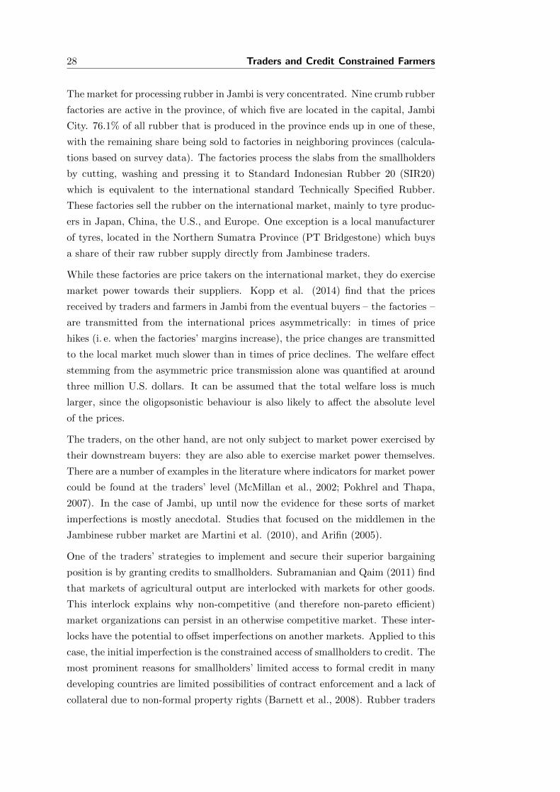
2.4 Lerner Indices of Jambinese rubber traders. . . . . . . . . . . . . . . . 39
3.1 Marketing channels for rubber. . . . . . . . . . . . . . . . . . . . . . . . 49
3.2 Intuition of asymmetric price transmission. . . . . . . . . . . . . . . . . 52
3.3 Symmetric error correction (continuous line) and asymmetric error cor-
rection (dotted line). . . . . . . . . . . . . . . . . . . . . . . . . . . . . 54
3.4 Welfare effect during adjustment process after shock at t=0 . . . . . . 56
3.5 Time series of buying and selling prices. . . . . . . . . . . . . . . . . . 58
3.6 Distribution of ect values. . . . . . . . . . . . . . . . . . . . . . . . . . 60
3.7 Penalized splines. . . . . . . . . . . . . . . . . . . . . . . . . . . . . . . 61
3.8 Results of one-dimensional grid search. . . . . . . . . . . . . . . . . . . 62
3.9 Correction of shocks over time. . . . . . . . . . . . . . . . . . . . . . . 64
4.1 Price development. . . . . . . . . . . . . . . . . . . . . . . . . . . . . . . 79
4.2 Welfare effects of policy changes. . . . . . . . . . . . . . . . . . . . . . . 79
4.3 Development of PM in ACP countries. . . . . . . . . . . . . . . . . . . . 83
4.4 Aggregate exports in millions of Euros. . . . . . . . . . . . . . . . . . . 88
5.1 Network structures. . . . . . . . . . . . . . . . . . . . . . . . . . . . . . 101
vii

List of Tables
1.1 Matrix of distortions and scales. . . . . . . . . . . . . . . . . . . . . . . 3
2.1 Spearman’s rank correlation coefficients between buying and selling
prices, and the traders’ positions in the value chains. . . . . . . . . . . . 27
2.2 Regression of estimated dry rubber contents on credits given. . . . . . . 35
2.3 Variables entering the production function. . . . . . . . . . . . . . . . . 35
2.4 Possible determinants of market power. . . . . . . . . . . . . . . . . . . 36
2.5 Regression results of revenue function. . . . . . . . . . . . . . . . . . . . 38
2.6 Determinants of market power that is exercised by traders. . . . . . . . 40
3.1 Estimates of long-run relation. . . . . . . . . . . . . . . . . . . . . . . . 60
3.2 Results of Akaike Information Critereon. . . . . . . . . . . . . . . . . . . 61
3.3 Results of all models discussed. . . . . . . . . . . . . . . . . . . . . . . . 63
4.1 Development of EU sugar policies. . . . . . . . . . . . . . . . . . . . . . 80
4.2 Estimation results. . . . . . . . . . . . . . . . . . . . . . . . . . . . . . . 89
viii


Chapter 1
Introduction
1

2 Introduction
1.1 Distortions on agricultural markets
For a long time, economic thought has been based on the assumption that efficient,
perfectly competitive markets are the normal case (Cassels, 1937), and that the best
policy is not to intervene in markets. This early assumption has, in many instances,
proven to not hold. Malfunctions do exist in various forms, and policy interference
is common. Agricultural markets are especially prone to malfunctioning due to a
number of characteristics specific to the sector. These include the wide geographical
spread of many small firms (Hallet, 1981) and relatively high levels of uncertainty
(Runge and Myers, 1985). Both lead to a greater volatility of output in agriculture
than in other sectors of the economy (Nedergaard, 2006). Hagedorn identifies a
systematic “economic disadvantage for the farm sector” (Hagedorn, 1983, p. 310):
the introduction of a new technology at the individual farm level does not lead to
an advantage in the market, but rather diverts disadvantages from the farm. This
is in contrast to the industrial sector, where a new technology usually enables the
generation of profits. The reason is a great homogeneity between producers and –
again – their large number (Hagedorn, 1983).
Gaining a deeper understanding of these distortions is crucial. A clear comprehen-
sion of the underlying mechanisms that result in a malfunction in a certain market
is the exclusive basis from which the best reaction can be developed. Likewise, it
is important to understand the effects of a certain policy, identifying the groups
of stakeholders who are actually affected, and anticipating their reaction. Agricul-
tural policies are influenced at an above-average level by lobby groups due to the
characteristics laid out above. The large number of rather homogenous producers
share very similar interests, fostering political coordination. The sector has in-
deed been successful in organising itself, as well as in influencing political processes
(Hagedorn, 1983). With deeper knowledge on these processes, an estimate of the
consequences to a society’s welfare from any distortion in agricultural markets can
be predicted, and eventually normatively assessed.
Two kinds of distortions observed on the markets of agricultural goods are discussed
in this work: a) the distortions that stem from a malfunction of the market, and b)
the ones that are policy-driven and have the target of changing the market outcome
(independent of whether market failure is present or not). The lack of market
functioning refers to non-competitive markets, i. e. the presence of market power on
either the demand side (mono-/oligopsony) or the supply side (mono-/oligopoly),
as well as to market failure.1
The market distortions are categorised according to their nature and along the
1Examples for each aspect of the theoretical framework are provided below.

1.1 Distortions on agricultural markets 3
scale dimension. A brief overview of the theoretical framework along which the
analyses are organized is presented in Table 1.1.
Table 1.1: Matrix of distortions and scales.
Scale
Micro Meso
Kind Market Malfunctioning on Sector-wide
of functioning disaggregated level malfunctioning
Distortion Policy Specific Sector-wide
Intervention measures interventions
Source: own production.
This introducing chapter provides the theoretical framework for the thesis, gives a
short summary of each of the three scientific articles, and puts them into a greater
context to highlight their relevance.
Target of this work
While there is a body of literature on market malfunctioning on the micro- and
the meso-/macro-scale, the scale dimension itself is often not explicitly expounded.
However, it makes sense to differentiate not only between the kinds of distortions,
but also along the scale dimension, since effects of micro-distortions (restricted to
one product, one market-segment, one geographic area, etc.) usually have imme-
diate effects at the local scale, but less tractable impacts at a more aggregated
scale. Likewise, the effects of distortions on a greater scale may trickle down to
the individual stakeholder at a quick rate, or on the other extreme, hardly be
recorded. A comprehensive report of market distortions must therefore account for
the differences in scale. This is not a negligible undertaking, since the functioning
of a market can be critically influenced by lower-level processes or constrained by
higher-level requirements. Examples can be found for every kind of distortion on
every level of aggregation. For the different combinations, examples are provided
in the course of this elaboration.
The choices made on the household level in a rural context are, for example, in-
fluenced by the social, economic, and legal environment. This framework of con-
straints and opportunities is present at all scales, be it local (customary) or national
law, socioeconomic indicators on a local scale or at the national level, such as tax-
ation, energy policy, or output prices on a global level (World Bank, 2007).

4 Introduction
The reconciliation of the meso-/macro-perspective with the understanding of mi-
croeconomic dynamics has been a challenge for economists of different sub-disciplines
during the last few decades (Kojima and Ozawa, 1984: foreign direct investment;
Chetty et al., 2011: labour supply; Robinson, 1991: structural adjustment; Bloom
and Canning, 2005: economic growth; Robilliard and Robinson, 2003: rural house-
hold income).
The target of this work is to discuss three of the four possibilities of the matrix
shown in Table 1.1 at one example, respectively. The key questions that each of
the papers attempt to answer by scrutinising the different kinds of distortions are
as follows: are market malfunctions present (chapters two and three)? What are
the distributional consequences: who wins and who loses? What are the net costs
to society? The replies to these questions are addressed in each of the papers, using
the examples of the rubber market in Jambi (Indonesia) and the European Union’s
(EU) sugar market order and will be condensed in chapter five.
1.2 Relevance and contribution
The agricultural sector is home to some of the most prominent examples of mal-
functioning markets. These markets malfunction due to a variety of reasons, such
as externalities or market concentration, for example. With the ‘industrialisation’
of the agricultural sector during the second half of the 20th century (e. g. mech-
anisation, increased application of synthetic fertilisers and pesticides, separation
of crop and livestock), its effects on the environment have increased tremendously
(Conway and Pretty, 1991). This can be observed both in industrialised and in
economically less developed countries. The industrialisation in agriculture led to an
increase of water and air pollution due to pesticides, fertilisers, residuals from on-
farm processing, and climate gas emissions, amongst others (Conway and Pretty,
1991). These externalities have the potential to affect the health of individuals
and the environment, and therefore the welfare of a given society. Market concen-
tration can be observed at many levels (e. g. the German beer industry, EU sugar
processors, or global dairy production) and often reduces total welfare (see below).
This is especially relevant in the context of economically less developed countries,
where markets exhibit imperfections on various levels. Since many farmers have
little bargaining power with their buyers, the increase of the total wealth to be
distributed (due to rising prices for agricultural products) does not necessarily lead
to increasing rural incomes. The resulting increased levels of inequality in rural
areas, which is contrary to the target of many rural development policies, lead in
turn to a higher pressure on the surrounding environment. A good example of this

1.3 Theoretical background 5
is poor households who engage in logging activities in areas covered by rainforest
(Dauvergne, 1993).
Policy intervention is also widespread in the agricultural sector – as a reply to
market failure, or as a measure of redistribution. The biggest part of the EU
budget, for example, has always been reserved for the Common Agricultural Policy.
One factor of it has been the Common Market Order for sugar.
Both kinds of distortions – failures and interventions – always create winners and
losers. This is independent of the total societal welfare. A distortion can cause an
increase, decrease or have no effect on welfare. This does not only depend on the
actual distributional effects of the distortion, but also on the underlying definition
of welfare, for example whether a certain amount of money is valued depending on
the income level of the group that holds it in their hands.
This dissertation contributes to the literature by presenting a review of distortions
of different scopes and scales. It includes two papers that broaden the horizon
concerning the (mal-)functioning of one specific market, covering the complex net-
works and interactions in great detail, and one piece that illustrates with a powerful
example how interventions can pile up until a complex system of (partly conflict-
ing) policies is built by policymakers under the pressure of the public, influenced
by lobbyists and constrained by obligations from multilateral agreements.
1.3 Theoretical background
Non-competitive markets
Gabszewicz and Thisse (2000) summarise the four conditions which have to be met
for a market to be competitive:
• The number of firms active in the market is sufficient in the sense that the
decisions of one firm do not have an influence on the market price (firm size
and number)
• No barriers exist for new (existing) firms to enter (leave) the market (free
entry/exit)
• Goods are homogeneous, leading to perfect substitutability between the prod-
ucts provided by two firms active on that market (product homogeneity)
• Every participant of the market has all information on the market prices of
all goods traded (perfect information)

6 Introduction
The discussion of underlying reasons for malfunctions on one specific agricultural
market presented in part 1.4 of this introduction goes along the lines of Gab-
szewicz’s and Thisse’s (2000) conceptualisation of these four characteristics of per-
fectly competitive markets.
Models that are based on the assumption of competitive markets have been criti-
cised for ’widen[ing] rather than to narrow the gap that has always existed between
the worlds of theory and of practice’ (Cassels, 1937). The first one to challenge
the assumption of competitive markets was Cournot in the book “Recherches sur
les principles mathemathiques de la theorie des richesses“ from 1838, in which he
introduced the concept of market power (Gabszewicz and Thisse, 2000). After
Cournot, there had been relative silence on the issue for nearly a century until the
‘Imperfect Competition Revolution’ took place in the 1920s and ‘30s (Gabszewicz
and Thisse, 2000). It was started by Piero Sraffa who rejected the concept of com-
petitive markets, stating that these are the exception rather than the rule (Sraffa,
1926). The reasons for his rejection are inconsistencies in the theory, as well as
contradictions with observations made in the real world. These inconsistencies and
contradictions refer to the fact that only a minority of enterprises/industries have
cost structures which fulfil the assumptions that the supply functions in economic
theory rely upon:
Business men [. . . ] would consider absurd the assertion that the limit to
their production is to be found in the internal conditions of production
in their firm, which do not permit of the production of a greater quantity
without an increase in cost. The chief obstacle against which they have
to contend when they want gradually to increase their production does
not lie in the cost of production [. . . ] but in the difficulty of selling
the larger quantity of goods without reducing the price. (Sraffa, 1926,
p. 543)
Instead, Sraffa understands the market not as a competition between identical
firms, but rather as one between many monopolies. Joan Robinson followed up on
that, and suggested a more general theory which incorporates perfect competition
as one special case (Robinson, 1959, first edition: 1933). At the same time, Edward
H. Chamberlin (1958, first edition: 1933) arrived at similar conclusions: consumers’
preferences towards single brands and willingness to substitute with similar (not
identical) products of another brand result in elastic demands faced by every sin-
gle firm, i. e. their decisions on production quantities influence the prices of their
products.

1.3 Theoretical background 7
As an empirical approach for analysing and quantifying market power, Structure-
Conduct-Performance (SCP) analyses of markets have been available since the
1940s (Schmalensee, 1989; Perloff et al., 2007). The ‘structure’ refers to the ob-
servable distribution of firms in a market, such as firm concentration and market
shares, as captured, for example, by the Herfindahl-Hirschman Index (Hirschman,
1964). The ‘performance’ indicates the proximity of the market outcome to the one
under perfect competition. ‘Conduct ’ stands for the behaviour of all stakeholders
active in the market, which is determined by the structure and results in the per-
formance. It is hence this unobservable element of the theory which connects the
observable characteristics of a market with the economic outcome.
More recent works have turned toward the modelling of decisions of economic
agents. Gabszewicz and Thisse (2000) observe an expansion of these game-theoretical
approaches since the 1970s. They summarise the game-theoretical implications of
the four conditions (that are presented above) which are to be fulfilled by a market
to be perfectly competitive. Perloff et al. (2007) differentiate between static and
dynamic models of game theory. While the static models assume that future devel-
opments have no effect on current decisions, the dynamic ones model the strategy
of agents who maximize not only current profits, but also the present value of future
profits. In the dynamic models framework, the current decisions can be based on
two motivations. The first one is the target to change the ‘fundamentals’ (i. e. the
future competitive environment), for example via investments into marketing, the
capital stock, etc. The alternative motivation is based on ‘strategic’ considerations.
They refer to actions that have the target to affect the belief of other firms about
the own behaviour in the future, such as the credibility of threats (Perloff et al.,
2007).
The analysis in chapter two is based on an SCP approach. Ideas for a more sophisti-
cated extension to the analysis conducted in chapter three with a game-theoretical
framework are laid out in chapter five.
Market failure
While Arthur C. Pigou did not invent the concept of externalities and market fail-
ure, he was the first to formally represent them in an economic model (Groenewe-
gen, 2009; Pigou, 1932). His concept of market failure associated with externalities
has been at the core of welfare economics ever since. Pigou assumed perfect com-
petition (Marcuzzo, 2009), so in his view market failure can be found in otherwise
perfectly competitive markets.
Externalities exist if the production or consumption of a good generates effects

8 Introduction
on other individuals which are not reflected in the product price. These effects
can increase other individuals’ utility or income (‘positive externalities’) or impose
costs on them (‘negative externalities’). The externalities do not need to take effect
at the point of time of their emission but may kick in with some delay. Typical
examples for negative externalities include soil and air pollution (delayed effect), or
noise (immediate effect), and for positive externalities bee-keeping and pollination
(immediate effect) or technology spillovers (delayed effect).
Another failure – apart from externalities – that can often be observed in rural areas
of economically less developed countries, is the lack of a (formal) capital market.
The reasons for the absence of a capital market lie firstly in the relatively high fixed
costs of establishing branches of formal lending institutions in rural areas; this is
primarily due to the fact that there are few potential customers per branch due to
low population density. Secondly, collateral is often not available, for example due
to a lack of formal land titles. Thirdly, the difficulty of acquiring information on
the potential borrowers, paired with low contract enforceability, increases the risk
of defaults.
It is important to note that failure in one market can be transmitted to another
market (Subramanian and Qaim, 2011). This is especially true for situations in
which markets are interlinked, as for example through complex networks of recipro-
cal exchanges in rural societies of low income countries (Ellis, 2000). One example
for these reciprocal exchanges can be found in the credit market. Ellis (2000) notes
that, especially in Asia, private sector money lending can often be found but is
often interlocked with other markets, which puts the borrower in a disadvantaged
negotiation position on the other market with the provider of his or her credit.
Other market characteristics leading to market failure include high transaction
costs, the existence of public goods due to non-excludability of consumers, govern-
ment corruption, the failure of the government to provide a stable currency, rule
of law, and the protection of property rights.2
Pigou’s concept of market failure also incorporates the maldistribution of income
and the creation of business cycles which result in instability in incomes and con-
sumption (Medema, 2009). Other authors, however, employ different definitions
of market failure. Following Koester (2011), for example, only divergences be-
tween the public and private willingness to pay qualify as failures of the market
mechanism while distributional considerations are not part of the concept.
2While these sources of market failure are mentioned here for the sake of completeness, theyare of limited relevance in the subsequent chapters, and are therefore not elaborated upon moreextensively at this point.
1.3 Theoretical background 9
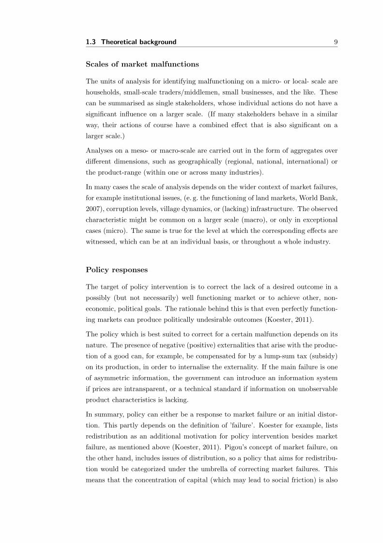
Scales of market malfunctions
The units of analysis for identifying malfunctioning on a micro- or local- scale are
households, small-scale traders/middlemen, small businesses, and the like. These
can be summarised as single stakeholders, whose individual actions do not have a
significant influence on a larger scale. (If many stakeholders behave in a similar
way, their actions of course have a combined effect that is also significant on a
larger scale.)
Analyses on a meso- or macro-scale are carried out in the form of aggregates over
different dimensions, such as geographically (regional, national, international) or
the product-range (within one or across many industries).
In many cases the scale of analysis depends on the wider context of market failures,
for example institutional issues, (e. g. the functioning of land markets, World Bank,
2007), corruption levels, village dynamics, or (lacking) infrastructure. The observed
characteristic might be common on a larger scale (macro), or only in exceptional
cases (micro). The same is true for the level at which the corresponding effects are
witnessed, which can be at an individual basis, or throughout a whole industry.
Policy responses
The target of policy intervention is to correct the lack of a desired outcome in a
possibly (but not necessarily) well functioning market or to achieve other, non-
economic, political goals. The rationale behind this is that even perfectly function-
ing markets can produce politically undesirable outcomes (Koester, 2011).
The policy which is best suited to correct for a certain malfunction depends on its
nature. The presence of negative (positive) externalities that arise with the produc-
tion of a good can, for example, be compensated for by a lump-sum tax (subsidy)
on its production, in order to internalise the externality. If the main failure is one
of asymmetric information, the government can introduce an information system
if prices are intransparent, or a technical standard if information on unobservable
product characteristics is lacking.
In summary, policy can either be a response to market failure or an initial distor-
tion. This partly depends on the definition of ’failure’. Koester for example, lists
redistribution as an additional motivation for policy intervention besides market
failure, as mentioned above (Koester, 2011). Pigou’s concept of market failure, on
the other hand, includes issues of distribution, so a policy that aims for redistribu-
tion would be categorized under the umbrella of correcting market failures. This
means that the concentration of capital (which may lead to social friction) is also

10 Introduction
understood as a market failure, which requires measures of redistribution from the
richer members of society to the poorest. Political goals in the agricultural sector
include, amongst many others, the conservation of a traditional lifestyle in rural
areas and self sufficiency of a particular region (Koester, 2011). Another possible
justification for a policy intervention is to rectify the (possibly unintended) side-
effects of older interventions, or the adjustment of a policy in anticipation of a
changed context. According to Constanza et al. (2001), one requirement that a
planned intervention has to fulfil is its social acceptance, i. e. the distributional con-
sequences, as well as its compatibility with international agreements. Many policy
instruments employed in agricultural markets have side effects, i. e. the influence
on markets other than the one primarily targeted with the intervention (Koester,
2011). As will be demonstrated later, this is not always given, and might therefore
require additional regulation. It will be of particular concern in chapter four.
Scales of policy interventions
Policy interventions in the agricultural sector can take two forms: a) regulative
laws – such as bans and rules – which are hereafter referred to as micro policies
or b) incentive based measures (Constanza et al., 2001). The latter market-wide
interventions are less specific and referred to as macro-policies hereafter. They
include measures such as subsidies, taxes, and quotas which are applied to pro-
duction, imports, or exports and have the potential to affect prices, as well as the
quantities that are produced and traded (Koester, 2011).
The micro policies (rules and bans) are very specific measures that are applied on
farm level. They concern production requirements and have to be followed by every
single farmer on each of his/her fields. Basically, all cross compliance regulations
of the Common Agricultural Policy (CAP), such as the fertilisation ordinance, the
direct payments obligation regulation (humus balance, green corridors, nitrogen
balance, crop rotation) fall into this category. It also includes measures that are
constrained by narrow geographical boundaries, such as the Bavarian corn root-
worm management regulation (“Maiswurzelbohrerbekampfungsverordnung”).
Both kinds of policies can have the target of redistribution or of correcting market
failure.
1.4 Application of the theoretical framework
Instead of providing systematic analyses of all cases (all possible combinations, all
aspects) included in the general framework, this work gives exemplary illustrations
for three of the general issues. Firstly, two cases of market failure are presented,

1.4 Application of the theoretical framework 11
both taking place in the Jambi Province on Sumatra, Indonesia. More specifically,
the illustrations relate to the rubber sector. Chapter two focuses on the underlying
dynamics at the micro-scale (village level), while chapter three delves into the
implications of a great concentration of this sector on a meso-level, i.e., at the
processor stage. These two cases are followed by one of policy intervention on a
meso-scale: The fourth chapter discusses the Sugar Market Order of the European
Union.3
The analyses carried out are based on quantitative research methods. Three ap-
proaches are applied as required by the different scales and scopes of the analyses:
in the first paper production functions are estimated, the second one follows a price
transmission approach, and in the third paper a gravity model is employed. More
information on the methodology is provided in the following subsections that are
dedicated to the individual articles. The different methodological approaches rep-
resented in the following three chapters also require the employment of different
kinds of data, so little can be generalised here: the most fundamental data that all
papers are based upon are information on trade flows, including traded quantities,
values, prices, and buyer-seller pairs. More exhaustive information on data and
their collection is provided in the respective sections.
Failures on the rubber market in Jambi, Indonesia
The Jambinese rubber value chain
Rubber production in Indonesia is predominately carried out by small scale farm-
ers. Their output consists of slabs of coagulated rubber of around 50kg.4 In the
Jambi Province on Sumatra Island, the vast majority of the rubber is delivered
to processors via a network of small- and medium-sized traders. The processors
– crumb rubber factories – clean and press the slabs into rubber blocks, follow-
ing the international product standard ‘Technically Specified Rubber’ (TSR). This
rubber is then exported all over the world for further processing, mainly in the tyre
industry.
Jambi is one example of a province that crucially depends on its agricultural sec-
tor. It also represents a typical rubber production area. 52% of the workforce is
employed in the agricultural sector and 48% of arable land is dedicated to rubber
production, of which 99.6% is cultivated by smallholders (Regional Account and
3The analysis of the EU CMO for sugar cannot be called a macro policy in the strict economicmeaning, since the focus is only on one sector of the economy. Nevertheless, the analysis is on avery aggregated level, and includes all countries that are active on the international sugar market.
4References to the information provided in these paragraphs can be found in chapters two andthree.

12 Introduction
Statistical Analysis Division, 2012). Although Jambi is not, on average, an excep-
tionally poor province, the rural population is still disadvantaged compared to the
populations in other parts of Indonesia.
The Jambinese rubber market is dominated by market power on the demand side
on all scales. The market structures tend to be oligopsonistic or monopsonis-
tic competition – the demand-side equivalents of monopolistic competition and
oligopoly. The processors exercise market power towards their suppliers (traders
and some large farmers), and the traders in the villages towards farmers and smaller
traders. Violations of all four preconditions for a competitive market as defined
by Gabszewicz and Thisse (2000) can be found at the different scales: symmetric
information, small firms, absence of entrance barriers, and product homogeneity.
Analysis on the micro scale has been carried out at the level of single individuals
via a representative survey of traders. The units of analysis at the meso-level are
the average price of five rubber processing firms and international prices.
Paper one: village level traders (micro scale)
When looking at the market performance on the micro scale, one can observe that
the prices paid by traders for their rubber input are below marginal value prod-
ucts (MVP). Varian (1987) describes first-degree price discrimination (or ‘perfect
discrimination’) of a monopolist as the selling of a product to each consumer at
the maximum price that he or she is willing to pay. By doing so, the monopolist
receives the whole possible rent, and the consumer none (note that under perfect
discrimination, the pareto-efficient quantity of a good is produced and sold). In
the case of demand sided market power, perfect discrimination means that the
monopsonist pays the lowest price for an input that each provider of this input
is willing to accept. Varian observes that “there are very few real-life examples
of perfect price discrimination” (Varian, 1987, p. 431). It might be the case that
the Jambinese rubber market is one of these rare examples, since most traders pay
different prices to each of their providers.
The structure of the Jambinese rubber market at the village level varies for different
geographic regions, but generally lies on the continuum between oligopsony and
monopsonistic competition. Bhaskar et al. (2002, p. 156) define monopsonistic
competition as an “oligopsony with free entry, so that [. . . ] profits are driven
to zero.” It is the demand-side equivalent to monopolistic competition as first
described by Chamberlin (1958). In some villages, true monopsonies can be found.
The results of the analysis carried out in chapter two show that the traders’ input
prices for rubber lie significantly below this input’s MVPs which is a strong indi-
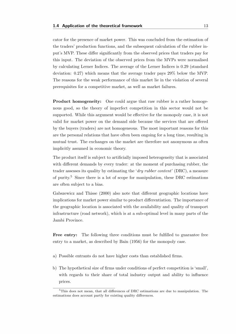
1.4 Application of the theoretical framework 13
cator for the presence of market power. This was concluded from the estimation of
the traders’ production functions, and the subsequent calculation of the rubber in-
put’s MVP. These differ significantly from the observed prices that traders pay for
this input. The deviation of the observed prices from the MVPs were normalised
by calculating Lerner Indices. The average of the Lerner Indices is 0.29 (standard
deviation: 0.27) which means that the average trader pays 29% below the MVP.
The reasons for the weak performance of this market lie in the violation of several
prerequisites for a competitive market, as well as market failures.
Product homogeneity: One could argue that raw rubber is a rather homoge-
nous good, so the theory of imperfect competition in this sector would not be
supported. While this argument would be effective for the monopoly case, it is not
valid for market power on the demand side because the services that are offered
by the buyers (traders) are not homogeneous. The most important reasons for this
are the personal relations that have often been ongoing for a long time, resulting in
mutual trust. The exchanges on the market are therefore not anonymous as often
implicitly assumed in economic theory.
The product itself is subject to artificially imposed heterogeneity that is associated
with different demands by every trader: at the moment of purchasing rubber, the
trader assesses its quality by estimating the ‘dry rubber content ’ (DRC), a measure
of purity.5 Since there is a lot of scope for manipulation, these DRC estimations
are often subject to a bias.
Gabszewicz and Thisse (2000) also note that different geographic locations have
implications for market power similar to product differentiation. The importance of
the geographic location is associated with the availability and quality of transport
infrastructure (road network), which is at a sub-optimal level in many parts of the
Jambi Province.
Free entry: The following three conditions must be fulfilled to guarantee free
entry to a market, as described by Bain (1956) for the monopoly case.
a) Possible entrants do not have higher costs than established firms.
b) The hypothetical size of firms under conditions of perfect competition is ‘small’,
with regards to their share of total industry output and ability to influence
prices.
5This does not mean, that all differences of DRC estimations are due to manipulation. Theestimations does account partly for existing quality differences.

14 Introduction
c) The products of the established firms do not have an advantage based on product
differentiation, such as brand loyalty.
For the monopsonistic case, condition b) is changed slightly (total industry output
becomes input), and conditions a) and c) are exchanged: condition a) requires pos-
sible entrants to face the same output prices as established firms, and in order to
fulfill c), the suppliers of the input should feel no loyalty towards the established
firms, but be able to freely switch to an entrant. In Jambi, condition a) is not
likely to be fulfilled because the access to rubber factories for selling is limited,
since supply is often larger than the factories can handle (see chapter three) and
the traders who have established personal relations are advantaged. It is difficult to
assess condition b) in general, since the concentration of the trading varies across
villages. Condition c) is certainly not fulfilled: the differentiation of demand is
based upon the ongoing personal relationship between seller and buyer (see elabo-
ration above). These close ties are amplified by the linkage of the trading business
with the credit market (see next point).
Credit constraint (failure): Since Jambinese farmers are constrained to receive
credit from formal lending institutions for the reasons laid out above (Ellis, 2000;
Subramanian and Qaim, 2011), traders assume the role of informal providers of
credit. For cultural reasons, the credit that traders provide to their suppliers
comes (predominantly) at a zero interest rate. Whether a farmer is indebted with
a trader, and - if yes - the size of the credit significantly affect the estimation of the
DRCs of the delivered rubber. As we will see, however, credits do not actually affect
the Lerner Index. This indicates that the correlation between DRC estimation and
credit given reflects only the traders’ own costs of providing liquidity in the form
of credit. This does not mean, however, that the DRC estimation is free from
manipulation on other grounds (see below).
Imperfect information: The costs for obtaining information on the prices that
different traders are paying for rubber are relative low for individual farmers. They
can be obtained via their personal networks, supported by mobile telecommunica-
tion technology. However, since the estimation of the DRC content is done on an
ad hoc basis and characterised by some arbitrariness, the farmer does not know
about it before selling to a new trader. The DRC estimations of his or her current
trader, on the other hand, can be predicted based on previous experience. The
farmer might have an idea of the distribution of possible DRC estimations given
by different alternative traders, but as demonstrated by Gabszewicz and Thisse
(2000), this information does not help and the trader can offer the monopson price.

1.4 Application of the theoretical framework 15
Market power (performance): Due to the nature of the product, the rubber
supply of an individual farmer, and thus the total supply on the market, is very
inelastic.6 This means that market-wide, there is a lot of scope for pricing be-
low marginal revenues. In a Bertrand-fashioned competition, traders are setting
the prices, and not the quantities (Bertrand, 1883, referred to in Gabszewicz and
Thisse, 2000). In essence, all the rubber that is available at a certain price will be
purchased.
For the analysis on the level of individual traders, the loyalty of providers needs to
be considered. They prefer continuing the business relationships with the traders
with whom they have established relations. This results in a willingness to accept
a certain price disadvantage. If the disadvantage exceeds a certain level, the farmer
might switch to another trader. From the trader’s perspective, the aggregation of
these behaviours of individual suppliers results in an upward-sloping supply curve
faced by the trader.
The aspect of perfect discrimination that was mentioned above could be imple-
mented via the manipulation of the DRC estimations which is different for every
farmer. However, it must be made clear that the estimation of the DRC is not
only determined by market power. The DRC reflects the de facto quality differ-
ences and is also systematically underestimated in order to recover credit costs,
and only partly according to non-observable characteristics of the farmer (which
would reflect his or her individual willingness to sell at a certain price).
Paper two: processors (meso scale)
As the second study (chapter three) reveals, the five crumb rubber factories lo-
cated in Jambi City exercise market power vis–a–vis their providers. A time series
analysis of co-movements of input- and output-prices shows that these processors
engage in asymmetric price transmission. Their market power manifests itself in
an intertemporal manipulation of marketing margins.
A look at the structure of the processing industry reveals at least monopsonistic
competition, in which “competition takes place among the few”, as Gabszewicz
and Thisse (2000) put it, or possibly even an oligopsony.
The identification of underlying dynamics is straightforward in this case. According
to Gabszewicz and Thisse (2000), established firms might find it profitable to erect
barriers against entry. These barriers can be of a technological nature, but may
also exist on a legal basis. This is the case for the Jambinese market of rubber
6This is only true for the short-term perspective. The production decisions (e. g. cultivationof rubber vs. oil palm) of farmers are taken as given and not subject to change within the timehorizon of this analysis.

16 Introduction
processing, where entry to the market (i. e. construction of another factory) is not
only very costly but actually impossible in the literal sense. While the barriers
to entering (or leaving) a market are frequently associated with high fixed costs,
in this case they are based on legislative grounds. The Jambinese factories have
an amount of political power which is great enough to deter the government from
permitting the establishment of new factories. Since these barriers are a success
of political lobbying, they are high investments/sunk costs. These costs would –
of course – not be incurred by new entrants if the market was free. In effect, this
artificially constrains the demand for the rubber (the number of factories is below
its optimal level), resulting in a price for the raw rubber input that is below the
optimal level.
The international rubber prices are provided by the Jambinese government, and
can be accessed via a mobile phone query (smartphones are not required). While
this is not very well known throughout the population in Jambi, it might not be
relevant for the suppliers’ assessment of the factory-prices anyway, since the facto-
ries’ processing costs are unknown to the suppliers. The prices that the different
factories pay for the rubber input is transparent to the providers, so the market
mechanism can be assumed to function in this respect.
The condition of product homogeneity is also fulfilled. The processing of rubber
in Jambi is homogenous in input and output, since no extra services are provided
to suppliers and all factories sell the same product, according to the international
standard TSR.
As mentioned above, the results of this analysis show that the rent that is redis-
tributed from the suppliers to the factories due to intertemporal marketing margin
manipulation is substantial: around three million U.S. Dollars are annually redis-
tributed from Jambinese farmers to factories. Compared to a non-oligopsonistic
market situation, the farmers have missed out on an income from rubber production
of 7%. The total redistribution that has been generated in the process could not
be quantified in this analysis (due to missing information on the price elasticities
on the supply and demand sides), but can be assumed to be substantial.
Methods and data
Paper one: The collection of the data required for this analysis was exercised
as a survey with agricultural traders in the Jambi Province from September until
December 2012. The targeted sample consists of all traders in 40 villages that are
representative for the rubber- and palm oil-producing regions in the province. A
response rate of 71% was achieved. The data obtained include prices and quantities

1.4 Application of the theoretical framework 17
of inputs and outputs, credit sizes given to individual farmers, as well as many other
business-related and personal characteristics of the respondents (see Appendix (3)).
Based on these data, a translog production function was estimated which was used
to calculate the MVP and subsequently the Lerner Indices. The Lerner Index
captures deviations of prices from the MVP. In a subsequent step, determinants of
this measure of market power were estimated.
Paper two: This paper employs an approach of time series analysis in order to
circumvent the problem of aggregating data over time which ignores the dynamic
nature of price setting processes. The analysis of price transmission enables the
assessment of the integration of markets. At the core of the empirical part of
this study lies the estimation of an Auto-Regressive Asymmetric Threshold Error
Correction Model. In order to understand the nature of the error correction process
without the need for restrictive a priori assumptions, the non-parametric estimation
technique of penalised splines is employed. The analysis is carried out based on
price data because they are – as in many other cases, too – the only data that are
available at the high frequency required for time series analysis. More specifically,
the factories’ buying and selling prices from 2009-2012 were used. The buying
prices were provided by GAPKINDO, the rubber processors’ association who collect
these data for their own purposes, and the selling prices stem from a Jakarta-based
marketing company which publishes the results of rubber auctions on a daily basis.
Policy interventions
Paper three: policy interventions on the EU sugar market (meso scale)
The third paper provides an example of a policy intervention designed to tackle a
market outcome that was not politically desired (or market failure, if one follows
Pigou’s definition of the same, which includes aspects of distribution). A gravity
analysis of monodirectional trade flows of sugar from all sugar producing countries
to the EU showed that countries that had been enjoying preferential access to the
protected European sugar market had been negatively affected by the reduction of
the intervention price for sugar between the years 2006 and 2009.
Behind the European sugar regime stands the political will to support producers
in the EU and in economically less developed third countries. The initial pol-
icy targeted the redistribution of rents from EU consumers to producers for sev-
eral reasons, including self-sufficiency (i. e. independence from imports from non-
community countries) and the support of rural livelihoods. As laid out above, a
policy intervention is justified if it enables the achievement of overall economic or

18 Introduction
sectoral policy targets (Koester, 2011). These measures of redistribution were then
also applied to formerly colonised countries, and subsequently also to the poor-
est countries in the world as a response to the non-desired market outcome of a
development gap between the Global North and South.7 These policies were im-
plemented via the Common Market Order (CMO) for sugar, followed by the Sugar
Protocol (SP), which is an annex to preferential trade agreements with the African,
Caribbean, and Pacific (ACP) countries, a conglomeration of formerly European
colonised countries, and eventually the Everything But Arms (EBA) agreement
with the Least Developed Countries (LDC) on earth.
The CMO for sugar consisted of an intervention price and a quota. So the bill for
the producer support was paid by European consumers, and partly by the European
taxpayer who had the burden to pay export subsidies because the sugar produced
under the quota, together with the imports from ACP countries and LDCs were a
multiple of what the domestic demand would absorb. The expected huge amount
of exports – caused partly by the introduction of unlimited access for the LDCs
– was the reason why the intervention price had to be strongly reduced over the
years from 2006 until 2009.
This reduction affected not only the European farmers, but also the ones that
were profiting from the high intervention price, too, namely the sugar producers
located in ACP countries. Since their preferential access lost part of its value,
this process is termed ‘Preference Erosion’. The work presented in chapter four
quantifies this erosion of preferences, as well as the impact of the changed CMO
on the other affected, non-European stakeholders. These are the LDCs, as well as
countries that are members of both the LDC and ACP groups. The results show
that Preference Erosion did occur. The ACP countries were indeed negatively
affected by the expected consequences of the introduction of the EBA.
Methods and data of paper three
The quantitative analysis is based on the empirically successful gravity model,
whose microeconomic foundation has been developed by Bergstrand (1985). The
estimation is carried out with the scale-independent Negative Binomial Quasi Gen-
eralised Pseudo Maximum Likelihood estimator in order to account for excess ze-
ros in the underlying data. These data include the monodirectional trade flows
in terms of values from all sugar producing countries to the EU, as well as other
variables required by the gravity specification, such as bilateral distance and mu-
tual resistance terms. Instead of capturing the policy via a dummy variable, the
7The terms ‘Global North’ and ‘Global South’ are used in this work as defined in Bendix et al.,2013.

1.4 Application of the theoretical framework 19
‘preference margin’ is employed in order to solve the problem of identification. It
measures the use that a country is making of its tariff-free quota. The data that
this analysis is based on stem from various sources. The allocated quotas and trade
quantities/values were provided by the European commission, the data indicating
political systems and distance between countries were generated by research in-
stitutes and information on total production quantities and exchange rates were
extracted from databases of international agencies.

Chapter 2
Traders and Credit Constrained
Farmers: Market Power along
Indonesian Rubber Value
Chains
21

Traders and Credit Constrained Farmers: Market Power
along Indonesian Rubber Value Chains
Thomas Kopp1 and Bernhard Brummer1
1Georg August University, Gottingen, Germany
Abstract
While traders of agricultural products are known to often exercise market
power, this power has rarely been quantified for developing countries. In
order to derive a measure, we estimate the traders’ revenue functions and
calculate the Marginal Value Products directly from them. We subsequently
find determinants affecting their individual market power. An exceptional
data set with detailed information on the business practices of rubber traders
in Jambi, Indonesia is employed. Results show that market power at the
traders’ level exists and is substantial. This market power is amplified in
situations of extreme remoteness, and weakens with increasing market size.
2.1 Introduction
It is widely recognized that traders and middlemen of agricultural raw products
are able to exercise a certain amount of market power, contradicting standard
economic theory of perfect arbitrage and zero profits (Aker, 2010; Subramanian
and Qaim, 2011; Piyapromdee et al., 2014). Osborne (2005) argues that the body
of literature on intermediaries of agricultural markets is extensive when looking at
the markets of industrialised economies. Southern markets, however, have rarely
been studied in this respect although it is to be expected that monopsonistic pricing
might be much more pronounced there: ‘traders in a typical source market engage
in imperfectly competitive behaviour in purchasing from farmers’ (Osborne, 2005,
p. 1).
Some newer studies address this gap in the literature and pay attention to the role
of traders. Most of these studies aim to find reasons behind the bad integration
of agricultural markets in economically less developed countries, while only a few
22

2.1 Introduction 23
base their analysis on information stemming from traders. Fafchamps and Gabre-
Madhin (2006) use data from a trader survey to quantify transaction costs, focusing
on the cost of information. Fafchamps and Hill (2008) record prices paid at several
stages of the value chain (including the farm gate) to collect evidence of market
power, leading to imperfect price transmission. The abovementioned study by Aker
(2010) analyses the effects of increased mobile telecommunication on the dispersion
of prices. Even fewer studies estimate traders’ production functions. Fafchamps
and Minten (2002) estimate production functions to quantify the effect of social
capital on the traders’ levels of productivity.
No study was found to use traders’ production functions for finding evidence of
market power. This might be due to several reasons: firstly, it is difficult to measure
the prices of the various outputs (i. e. services) offered by these individuals, such as
changing the location of a good, or of providing credit. Besides that, in many cases
the data on firms’ individual output prices is not available at the level of detail
required (Mairesse and Jaumandreu, 2005).
Our study investigates traders’ market power by comparing the marginal value
products (MVPs) of the agricultural raw input to their observed market price.
A unique set of original survey data on Indonesian rubber traders – including
detailed output prices on an individual level – enables us to estimate the traders’
revenue functions and calculate the MVPs directly from them. The comparison
to the observed market price is operationalised by calculating Lerner Indices (the
normalised difference between market and observed prices) which are shown to be
significantly different from zero. The traders exercise monopsonistic market power.
In a subsequent step, we search for determinants that influence this market power.
Our results suggest that market imperfections such as high transaction costs (typ-
ical for remote areas) increase the imbalance. Factors that reduce the traders’
ability to exercise power are the size of the market, such as the agricultural area
dedicated to cash crop production, and the number of traders operating in the area.
This paper is structured as follows: the data used in this study is introduced in
section two. Section three provides background information on the Jambinese rub-
ber market and the business practices of the subjects of this analysis – the traders
and middlemen. The empirical methods are discussed in section four. Section five
presents the results, before conclusions are drawn in section six.

24 Traders and Credit Constrained Farmers
2.2 Data
The data that this study is based on were generated during a survey taking place
from September to December 2012 in five districts of the Jambi Province on Suma-
tra, Indonesia in a joint project between the universities of Gottingen, Jambi, and
Bogor.1 These five districts are the primary production areas of rubber in Jambi.
In these five districts, 40 villages were selected randomly, stratified on a sub-district
level (Faust et al., 2013). The total population of rubber traders in these 40 villages
could be determined by a snowball-like search in the survey phase and totals to 313
individuals. Out of these, 221 were interviewed, which is equivalent to a response
rate of 71%. All prices, values, and quantities refer to September 2012. Since the
figures mainly stem from accounting documents of the respondents, a high level of
accuracy can be assumed (if no accounting was available, we relied on recall data).
The traders were asked about details of the three most important suppliers and
buyers whom they source from and deliver to, respectively. It is safe to assume
that this covers all their buyers because 99% of the respondents sell to only one or
two.
2.3 Background: rubber in Jambi
Why did we select rubber and the Jambi province? The fact that raw rubber has a
high value per volume compared to other raw products and is not perishable makes
it an extensively traded good that can be moved along complex value chains. Jambi
is representative of a rubber producing province in Indonesia, the second largest
producer in the world (see figure 2.1).2 Rubber is also important for the Jambi
province in particular and is seen by policy makers as one key for reducing unem-
ployment and poverty (Feintrenie et al., 2010). This all makes it an interesting case
study for the application of the proposed method of estimating revenue functions
in order to find evidence for market power.
Today, rubber is the main commodity produced by smallholders in Jambi. Jambi
is a key producer of palm oil too, but a lot of this production takes place in the
form of large scale plantation agriculture while rubber is predominantly produced
by smallholders. Martini et al. (2010) argue that a mixed portfolio of rubber
and palm oil would be the best strategy for smallholders to insure against price
volatilities on both markets and provide an income which can keep up with wages
1Collaborative Research Centre 990: http://www.uni-goettingen.de/en/310995.html. Wethank Jenny Aker (Tufts University), Todd Benson (IFPRI, Kampala), and Ruth Vargas Hill(IFPRI, Washington) who were so kind to provide the blank questionnaires they used for theirrespective trader surveys.
2Figure based on data from FaoStat (accessed on 08.10.2014).

2.3 Background: rubber in Jambi 25
Figure 2.1: Global rubber production in 2012.
earned from providing labour in the cities. It can be observed, however, that
the Jambinese population generally seems to prefer rubber. With 250 000 rubber
producing households, 31% of all Jambinese livelihoods rely on rubber (Statistics
of Jambi Province, 2013). Policy makers also agree that rubber cultivation plays a
key role for Jambi’s future economic and social development. In contrast to palm
oil, its primary production mode is smallholder agriculture because of the labour
intensity. Rubber production’s compatibility with food production increases food
security as rubber can be intercropped with food crops such as rice, vegetables, and
fruit (Feintrenie et al., 2010). This is especially true in the current time of land
pressure. However, at present this is rarely exercised (Euler et al., 2012). Even
larger scale rubber plantations have weaker negative environmental externalities
than palm oil monocultures, for example on biodiversity (Fitzherbert et al., 2008)
and the probability of flooding (Adnan and Atkinson, 2011).
In Jambi, the stakeholders in rubber trade (middlemen and agents of other traders)
are heterogeneous along several dimensions and form complex networks (see Figure
2.2). Traders can either be independent entrepreneurs or agents working for a larger
trader. The latter are referred to as Anak Ular (‘children of the snake’) which
indicates their low popularity and perceived powerful position. The traders in our
sample differ considerably in business size (trading between 300 kg and 200 tons
per week, and buying regularly from 3 to 800 providers) and other characteristics,
such as ethnicity, age, etc.
The buying procedure works as follows: the trader either lives in the village, or
comes to the village at a fixed point in time (e. g. one day per week) to buy rubber.
In either case, the rubber provided by the farmers comes in the form of a slab
of coagulated rubber of 50-100 kg. The rubber is then typically weighed by the
trader’s employees before the trader assesses its quality by calculating the Dry

26 Traders and Credit Constrained Farmers
Figure 2.2: Trade flows of rubber in the Jambi Province.
Source: Own production, based on original survey data. Borders of Jambi andSumatra from Center for International Forestry Research, surface of Jambi fromNASA/EOSDIS.
Rubber Content (DRC). The ideal DRC would be 100%, but is most commonly
graded down for several reasons. First is the basi content which refers to the
contamination with water. Most farmers increase their rubber slabs’ weight by
storing them in water pools to make the slabs soak up water like a sponge. The
second contamination is in the form of tatal (‘rubbish’) from the harvesting process,
such as leaves, bark or dirt from coagulation boxes. Finally, the chemical that
has been used for coagulation also affects the quality. While the highest quality is
achieved with acetic acid, many farmers use cheap alternatives such as battery acid,
triple super phosphate fertilizer, vinegar, or even floor cleaner (Akiefnawati et al.,
2010). It has to be noted that the terms basi and tatal are used interchangeably
and some people may never have heard of one of them. However, all three kinds
of quality determinants are known, and most commonly referred to in the way
explained above. In this work, we use the term DRC to refer to all quality aspects
combined. Traditionally the farmers produced sheets of unsmoked rubber, but
had to switch to the production of thick slabs due to policy changes in the early
1970s, after which only the export of Technically Specified Rubber was allowed

2.3 Background: rubber in Jambi 27
and lower grades were prohibited (Pitt, 1980). The disadvantage from the farmers’
perspective is that the quality of unsmoked rubber sheets is less variable than the
quality of slabs, which are therefore more prone to manipulation.
The downstream trading network (i. e. for selling the rubber) is very dense and
complicated as one can observe in Figure 2.2 (above). When moving along the
value chain from the village trader, the product passes on average 3.1 other traders
before reaching the factory (dispersion: see Figure 2.3). While the prices that the
middlemen receive for the product traded depend on their position in the chain, the
prices that they pay do not (see Table 2.1). The fact that the prices received from
selling rubber downstream are not transmitted to the providers shows that some
traders are not operating at their marginal costs. This is already a first indicator
of the traders acting as price setters.
Figure 2.3: Position of respondents in the value chain, starting from the factory.
Source: Own production, based on original survey data. Number three indicates,for example, that the produce passes two other traders before reaching the factory.Decimal values are possible, because averages were taken for traders who sell alongmore than one downstream channel, if these differ in length.
Table 2.1: Spearman’s rank correlation coefficients between buying and sellingprices, and the traders’ positions in the value chains.
Variable A Variable B p-value (H0: Variable A andVariable B are independent)
selling price pos in chain 0.0871buying price pos in chain 0.3748
28 Traders and Credit Constrained Farmers
The market for processing rubber in Jambi is very concentrated. Nine crumb rubber
factories are active in the province, of which five are located in the capital, Jambi
City. 76.1% of all rubber that is produced in the province ends up in one of these,
with the remaining share being sold to factories in neighboring provinces (calcula-
tions based on survey data). The factories process the slabs from the smallholders
by cutting, washing and pressing it to Standard Indonesian Rubber 20 (SIR20)
which is equivalent to the international standard Technically Specified Rubber.
These factories sell the rubber on the international market, mainly to tyre produc-
ers in Japan, China, the U.S., and Europe. One exception is a local manufacturer
of tyres, located in the Northern Sumatra Province (PT Bridgestone) which buys
a share of their raw rubber supply directly from Jambinese traders.
While these factories are price takers on the international market, they do exercise
market power towards their suppliers. Kopp et al. (2014) find that the prices
received by traders and farmers in Jambi from the eventual buyers – the factories –
are transmitted from the international prices asymmetrically: in times of price
hikes (i. e. when the factories’ margins increase), the price changes are transmitted
to the local market much slower than in times of price declines. The welfare effect
stemming from the asymmetric price transmission alone was quantified at around
three million U.S. dollars. It can be assumed that the total welfare loss is much
larger, since the oligopsonistic behaviour is also likely to affect the absolute level
of the prices.
The traders, on the other hand, are not only subject to market power exercised by
their downstream buyers: they are also able to exercise market power themselves.
There are a number of examples in the literature where indicators for market power
could be found at the traders’ level (McMillan et al., 2002; Pokhrel and Thapa,
2007). In the case of Jambi, up until now the evidence for these sorts of market
imperfections is mostly anecdotal. Studies that focused on the middlemen in the
Jambinese rubber market are Martini et al. (2010), and Arifin (2005).
One of the traders’ strategies to implement and secure their superior bargaining
position is by granting credits to smallholders. Subramanian and Qaim (2011) find
that markets of agricultural output are interlocked with markets for other goods.
This interlock explains why non-competitive (and therefore non-pareto efficient)
market organizations can persist in an otherwise competitive market. These inter-
locks have the potential to offset imperfections on another markets. Applied to this
case, the initial imperfection is the constrained access of smallholders to credit. The
most prominent reasons for smallholders’ limited access to formal credit in many
developing countries are limited possibilities of contract enforcement and a lack of
collateral due to non-formal property rights (Barnett et al., 2008). Rubber traders

2.4 Methodology 29
are traditionally providers of informal credit. Observations of our survey showed
that no collateral is needed because the credit agreement is based on trust, stem-
ming from ongoing personal interaction and close ties within the village community.
This confirmed the observations made by Akiefnawati et al. (2010). However, this
credit also increases the traders’ bargaining power tremendously, since it is ex-
pected that an indebted farmer sells his or her produce exclusively to the provider
of his or her credit. This strategy has also been reported in the cases of Benin and
Malawi: the credit’s ‘[. . . ] main purpose is not to exploit farmers’ need for cash
in order to finance agricultural production, but rather a means for traders to se-
cure future deliveries’ (Fafchamps and Gabre-Madhin, 2006, p. 36). This behaviour
could also be documented for the case of Jambi: 94.1% of the rubber traders who
provide credit answered ‘yes’ to the question ‘Does a farmer have to sell his/her
rubber/palm oil to you if he/she wants to take a credit from you?’. 72.9% replied
with ‘no’ when they were asked: ‘If a farmer/other trader owes you money, can
she sell her produce to another trader?’ (All figures for this and the following
paragraph are based on original survey data; for more information on the data see
above).
The credit not only attaches the farmers to the traders, but these traders also
manipulate the DRC level of the delivered rubber if the farmer is indebted. This
would be an implicit interest since, for cultural reasons, the traders do not officially
charge any interest on the credit. In interviews, 11.8% of the responding traders
stated that they manipulate the basi estimation for suppliers who are indebted.
This seems to be a small share, but given that this practice is understood as
immoral, it can be expected that the figure given here is underestimating the
true share because respondents might not ‘admit’ in interviews that they follow
this practice. However, it is reasonable to understand this hidden interest as the
traders’ own capital costs which they pass on to the farmers.
It is the target of this analysis to empirically verify whether Jambinese rubber
traders do indeed exercise market power towards their suppliers and – if so – what
determines the extent of it. The key question is whether factor prices of the rubber
input equal their marginal value products.
2.4 Methodology
The intuition of our empirical approach to test for market power at the traders’
level is to estimate the revenue functions of the traders. We use these estimated
functions to directly calculate the marginal value product (MVP) of raw rubber
which would– in the situation of perfect competition – be equal to the observed

30 Traders and Credit Constrained Farmers
market prices that the traders pay for this input. If the latter ones were smaller,
this would be an indication of market imperfection. In a second stage, we find
determinants for deviations from the MVP by calculating Lerner Indices for each
trader, and regressing them on characteristics of the transactions (characteristics
of the geographic location, of the traders, and of the trader-provider relationships).
Model development
Berndt (1996) argues that in situations of exogenous input quantities and endoge-
nous input prices, the production (or revenue) functions need to be employed.3
The advantage over estimating a cost function is that input prices do not enter
the model which we wish to avoid, since these are the observed prices that are to
be compared to the MVPs deducted from the estimated revenue functions. ‘Pro-
duction’ is, in this case, understood as improving the value of the raw rubber that
the traders buy, for example by changing its location, i. e. providing the service of
transportation. Since the selling prices of rubber which the traders are confronted
with vary substantially between the traders – depending on whom they sell to –
the standard approach of generating the output quantity by dividing the revenue
by an industry-average of the prices would not account for these price differences
and therefore lead to a serious bias (Mairesse and Jaumandreu, 2005). Instead we
weight the output by the selling prices, resulting in the estimation of a revenue
function. Mairesse and Jaumandreu (2005) find that it does not systematically
change the estimated results if the LHS of a production function is deflated by the
output prices or not (apart from the desired effect from the weighting).
A potential problem in the estimation of traders’ production functions is one of
endogeneity: traders who are generally more efficient might handle larger volumes,
which would cause a correlation between the error term and this input quantity.
However, in Jambi it is not the trader’s choice how much rubber he or she trades,
since they usually buy everything they can get. According to Zellner et al. (1966),
the problem does not apply if the choice of how much input is used is not made
by the trader. The same is true for the credit: the amount of the credit that the
traders provide is determined by their providers’ needs rather than their own choice.
The credit is, as in other settings, too (e. g. Benin and Malawi, see Fafchamps and
Gabre-Madhin, 2006), used as an instrument to attach providers to them. Thus
the output/revenue per input is not correlated to the total quantity moved by the
3The reason why we do not estimate a value added function is that knowing which factors affectthe value-added would not facilitate any conclusions on market power. It would be interestingto assess how the value added is distributed amongst all stakeholders of the value chain, but thisis not feasible within the scope of this study since it would require detailed data on the coststructures of all stakeholders.

2.4 Methodology 31
trader.
Application
We base the specification of our model on the following transcendental revenue
function in logarithmic form (Boisvert, 1982):4
lnY = lnα0 +
N∑i=1
(αi lnxi) +1
2
N∑i=1
N∑j=1
(αij lnxi lnxj) + ε (2.1)
Y on the LHS represents the value of the output while the xi on the RHS refer
to the quantities of the inputs. N denotes the total number of inputs and ε the
error term. For the reasons laid out above, the output enters in the form of gross
revenue. The raw rubber that the traders buy is included as an intermediary input.
Other variables that are included in the RHS are the bilateral distance between the
trader and his or her buyer as a proxy for trade costs, the weekly hours that the
traders work themselves, and their total transport capacity as a proxy for capital.
Concerning the costs of hired labour, it cannot be deduced from theory if they are
to be modelled in terms of working hours or total costs: the price of labour might
account for unobserved quality differences which would argue for using the total
costs. However, price differences might also be due to regional differences which
would be a reason for using the amount of working hours. The latter two variables
cannot enter the regression together due to double counting. We therefore estimate
three models: one without hired labour (1), one with the total labour costs (2),
and one with total hours worked (3). An F-Test is then employed to compare (2)
and (3) with (1). If the reduced model is shown to represent the data best, its
results are used further on. If the models that include the hired labour are better
than the one without it, the Vuong’s Closeness Test for non-nested models (Vuong,
1989) will be employed to determine whether to use (2) or (3).
The traders produce – from their suppliers’ point of view – two services: changing
the location of the product and providing credit. However, since from the traders’
perspective their sole motivation of providing credit is to expand their market base
and to attach providers to them, this is to be understood as a (quasi-fixed) input.
Thus, the credit enters the regression on the RHS, together with the other inputs.
The DRC does not enter the revenue function, since the input amount is equal to the
output amount. This means that on the LHS the quantity is already deflated by the
4We also estimated a Cobb Douglas function. An F-test showed that it does not represent thedata as good as the translog specification. Results are available on demand.

32 Traders and Credit Constrained Farmers
output quality which is equal to the (weighted) average input quality. Accordingly,
there is no need to control for this in the revenue function.
Before taking the logarithms of all variables, they are mean-scaled which enables the
interpretation of the results as elasticities. One common challenge in the estimation
of revenue functions is the occurrence of zeros in the input variables which results in
missing values when the log is taken. This is the case – for example – if a very small
trader does not make use of hired labour. These missing zeros are handled following
Battese (1997): the observations with ln 0 are replaced by 0. An additional dummy
variable, which represents the zero-inputs, is set to one in these cases, and to zero
otherwise.
The variable indicating the credit that the respective trader provides is zero in-
flated and left censored (about 50% of the respondents did not give any credit in
September 2012). So instead of normalising and taking the logs of this variable,
the inverse sine hyperbolic transformation was employed, as suggested by Burbidge
et al. (1988). Since the size of the credit given by traders is not exclusively deter-
mined by their choice, but also based on their providers’ needs, it is also plausible
to represent the credit as a dummy variable (one if credit was given). This speci-
fication was tested against the alternative of treating the credit given just like the
other inputs via an LR test which gave a prob> chi2 of 0.0771. It was therefore
decided to employ the unrestricted model.5
Requirements and properties of the revenue function
We test whether the estimated revenue function satisfies the required properties at
each data point. These are the homogeneity condition (Boisvert, 1982), as well as
the curvature properties for satisfying the conditions of positive and diminishing
marginal products for every single observation (Morey, 1986). The condition of
positive marginal products is checked by taking the partial derivatives with respect
to each of the inputs. If they are > 0 at every data point, the first condition is
fulfilled. The decreasing marginal products are clarified by taking the second-order
partial derivatives with respect to each of the inputs which is the diagonal of the
bordered Hessian matrix (Morey, 1986). These need to be < 0 at every observation
in order to satisfy the condition. As it will turn out, the application of a standard
OLS estimator produces estimates which violate the constraints 760 times. We
thus impose the inequality constraints mentioned above, following the approach
suggested by Henningsen and Henning (2009) using the R-packages micEcon and
frontier.6 For the first step, we estimate the unrestricted translog revenue function
5The results of the alternative model can be made available upon request.6A list of the imposed constraints can be found in Appendix (1).
2.4 Methodology 33
before imposing the monotonicity constraint by minimum distance in the second
step. In the third step, the non-restricted parameters are estimated conditionally
on the restricted parameters. Imposing the constraints on every single point in the
data is not desirable, because this would eradicate the flexibility of the transcen-
dental logarithmic (translog) revenue function, and one would be left with a Cobb
Douglas function. In order to keep the advantage of the translog specification, we
impose the constraints for only one arbitrarily chosen point, as suggested by Ryan
and Wales (2000) and applied by Chua et al. (2005). We select the sample mean
to be this point. Imposing the monotonicity condition already significantly reduces
the number of data points that violate the revenue function’s curvature properties
to twelve cases (quasi-concavity achieved in 94.3% of all observations).
Calculation of Marginal Value Products
In order to calculate the MVPs, Equation (2.1) is differentiated with respect to
ln(xR):7
∂ lnY
∂ lnxR= αR + αRR lnxR +
M∑j=1
(αRj lnxj)
(2.2)
Substituting the assumption of perfect competition ∂Y∂xR
= pcR and the equality8
∂Y∂xR
= ∂ lnY∂ lnxR
YxR
into (2.2) yields
pcR =
αR + αRR lnxR +
M∑j=1
(αRj lnxj)
Y
xR(2.3)
with pcR representing the price under perfect competition. In the subsequent step,
the Lerner Index is calculated for each trader. The original formula normalises the
positive difference between marginal costs and observed prices (i. e. prices minus
marginal costs, since the former ones tend to be larger) by the observed prices
(Lerner, 1934). Since we are comparing the marginal revenues and factor prices,
we calculate the index as LI =pcR−p
∗
p∗ with p∗ standing for the observed price.
Determinants
In the second stage regression, the calculated Lerner Indices from stage one are
regressed on several characteristics of the traders’ environment in order to find
determinants of the market prices’ deviations from the competitive prices. These
7note: M = N\R8Steps: with (a) ∂ ln y/∂y = 1/y and (b) ∂ lnx/∂x = 1/x, the equality is given by (a) / (b).

34 Traders and Credit Constrained Farmers
characteristics are differentiated between proximate causes (variable, such as mar-
ket and trader characteristics), and ultimate causes (stable over time, such as char-
acteristics of the geographic location). The former ones include the trader density
in the survey village, the traders’ ‘size’ (their wealth and trading quantity), their
respective positions in the value chain, their access to information, their access to
capital (credits), and their status (agent or independent trader). Unobserved trader
heterogeneity is controlled for by adding a dummy for each trader. Ultimate causes
include the general remoteness, size of village population, the quantity of rubber
production, availability of lending institutions or an auction market, as well as the
participation in the governmental ‘transmigration’ program. The heterogeneity of
the providers, from whom the traders under consideration source the rubber, is
controlled for with the following variables: the provider’s status as farmer/other
trader, the typical size and quality of delivery, their ethnicity, and the credit that
has been taken. We test for heteroscedasticity with the Breusch-Pagan Test, which
is confirmed. We thus use robust standard errors.
Since output quality is equal to the (weighted) average input quality, the hypothet-
ical input price is for rubber of average quality. However, there is heterogeneity
between farmers whom the traders buy from. As mentioned above, traders are
accused of manipulating the estimation of the DRC for indebted suppliers. This
accusation could be verified by a regression of the estimated DRC on the size
of credits which were given out to farmers (Table 2.2). In case of zero-credits,
log credits takes the value 0 and the dummy of credits given is also set to 0, follow-
ing Battese (1997). As can be seen, the credit that is given does indeed influence
the DRC. The low R2 can be explained by the fact that the main determinant of
the DRC estimation is still the quality. However, the variables representing the
credits are significant. To account for this in the estimation of the possible deter-
minants of market power, we generated the credit adjusted quality as the residuals
from regression (4) in Table 2.2. The variables that enter the estimation of the
revenue function are listed in Table 2.3.
In order to identify drivers of market power in the Jambinese rubber markets, each
trader was asked for detailed information on three arbitrarily selected providers.
These, together with characteristics of the trader him/herself, as well as charac-
teristics of the market that they are operating within are used in the second stage
regression (Table 2.4). The value of the respondent’s house is an indicator of his/her
wealth. The variable ‘Informal credit ’ refers to a money-lender or a rubber-trading
warehouse that provides credit to suppliers. ‘General remoteness’ represents the
average distance between the respondent’s location and the crumb rubber factories
that can be accessed by the Jambinese traders. The number of households of each

2.5 Results and discussion 35
Table 2.2: Regression of estimated dry rubber contents on credits given.
(1) (2) (3) (4)VARIABLES Credit Size Dummy Dummy Village
and Credit DummiesSize Added
log credits 0.0711* -0.170 0.168**(0.0407) (0.153) (0.0757)
dummy credit given 1.211** 3.516 -2.588**(0.572) (2.154) (1.050)
Constant 5.388*** 5.307*** 5.307*** 10.000***(0.324) (0.327) (0.327) (1.829)
Observations 666 666 666 666R-squared 0.005 0.007 0.009 0.803
Standard errors in parenthesesCoefficients of village dummies in (4) are not reported
*** p<0.01, ** p<0.05, * p<0.1
Table 2.3: Variables entering the production function.
Variable Label Mean Std. Dev.
YR Value of rubber sold (IDR) 1.29E+08 2.74E+08x1 Quantity of rubber traded (kg) 10324.5 19175.12x2 Respondent’s weekly working hours 17.70894 19.08984x3 Transport capacity (kg) 2292.569 4293.935x4 Distance to buyer (km) 62.34715 97.34556x5 Monthly costs of hired labour (IDR) 1824851 3812094x6 Weekly working hours of hired labour 22.01606 43.53851x7 Credit given to all providers (IDR) 1.88E+08 1.35E+09
village, as well as the agricultural area that is not dedicated to rice production
were drawn from the PODES2008 dataset.
2.5 Results and discussion
First stage regression
The results of the first stage regression are presented in Table 2.5.9 It has to be
kept in mind that this estimation was done at the trader level, i. e. each observation
9x R = rubber input, x 1 =respondent’s working hours, x 2 =transport capacity,x 3 =distance to buyer, x 4 =hired labor, costs, x 5 =hired labor, hours, x 6 =all credit given.

36 Traders and Credit Constrained Farmers
Table 2.4: Possible determinants of market power.
Variable Label Mean Std. Dev.
Lerner Index Lerner Index 0.502913 0.338702number traders karet Number of rubber traders in village 12.445 5.533log house cost Value of respondent’s house 18.483 1.335providing farms Number of farms that respondent buys from 34.005 40.646providing traders Number of other traders that respondent buys from 1.294 7.445pos in chain traders Respondent’s position in the value chain 3.061 0.564transmigrasi village Dummy for ’Transmigrasi’ village 0.317 0.465general remoteness General remoteness of respondent 161.614 15.269dist to closestfactory Distance to closest rubber factory 21.223 14.469households in village Number of households in village 676.147 385.153no podes2008 data no info on village characteristics 0.0367 0.188agric area non rice Agricultural area, non-rice 5626.314 5734.092formal credit available Availability of formal credit institutions 0.312 0.464informal credit available Availability of informal credit institutions 0.037 0.188credit mio Debt of provider with respondent (in mio. Rupiah) 1.383 5.576quality credit adjusted Credit-adjusted quality of delivered rubber 93.510 7.044little information Respondent’s access to information is restricted 0.464 0.499discuss prices Respondent discusses prices with other stakeholders 0.649 0.478price agreements Respondent agrees on prices with other stakeholders 0.212 0.409ethnic resp java Respondent’s ethnicity is Javanese 0.425 0.495
is equivalent to one trader in the sample.
The DRC does not enter this estimation because the estimation is executed at the
trader level. The quality of the output is equal to the average input of the input.
The manipulation of the basi estimation is just one strategy of pushing down the
input price towards the monopson price.
Model choice
The F-Tests indicate that the model which omits hired labour is superior to the
models including hired labour in the form of working hours or total costs, respec-
tively; both null hypotheses of the restricted model to represent the data better
cannot be rejected (test results are 90.3% and 65.7%, respectively). This obser-
vation is robust against changes in all model specifications which we have exper-
imented with.10 We thus assume that model (1) of Table 2.5 represents the data
best. Column (2) shows the results of the estimation based on the same choice of
regressors as column (1), with the constraints on the curvature properties being
imposed. Standard errors are not reported because their calculation would be bi-
ased since the regression is subject to constraints. For the second stage we use all
10Results for other specifications are available on demand.

2.5 Results and discussion 37
coefficients from column (2). The data used in the revenue function estimation have
been cleaned for outliers (9 observations out of 218 were dropped). If the outliers
are included, the estimated coefficients are not very different, but fewer are statis-
tically significant. The F-Tests indicate that the model which omits hired labour
is superior to the models including hired labour in the form of working hours or
total costs, respectively; both null hypotheses of the restricted model to represent
the data better cannot be rejected (test results are 90.3% and 65.7%, respectively).
This observation is robust against changes in all model specifications which we
have experimented with.11 We thus assume that model (1) of Table 2.5 represents
the data best. Column (2) shows the results of the estimation based on the same
choice of regressors as column (1), with the constraints on the curvature properties
being imposed. Standard errors are not reported because their calculation would
be biased since the regression is subject to constraints. For the second stage we use
all coefficients from column (2). The data used in the revenue function estimation
have been cleaned for outliers (9 observations out of 218 were dropped). If the
outliers are included, the estimated coefficients are not very different, but fewer
are statistically significant.
It comes as a surprise that the production factor ‘hired labour ’ does not play a role
in the revenue generating process. The explanation for this lies with the fact that
the hired labour input is relatively unimportant, compared with the other inputs,
since many traders do not rely on paid labour at all.
Calculation of price deviation
Figure 2.4 shows the distribution of the calculated Lerner Indices. They indicate
the percentage-deviation of the price that is paid from the MVP. If these values
are equal, the Lerner Index takes the value 0. The average of the Lerner Indices
is 0.29 (standard deviation: 0.27) which means that the average trader pays 29%
below the MVP. The fact that the prices that most traders pay for their rubber
input is far below this input’s MVP is a clear indication for market power.
Second stage regression
Table 2.6 shows the results of the second stage regression that evaluates determi-
nants of the level of market power exercised by the surveyed traders. The number
of observations is larger than in Table 2.5 because, in this case, the regression was
done on a further disaggregated level. This was accomplished by integrating up
to three different providers who the traders source from as separate observations.
11Results for other specifications are available on demand.

38 Traders and Credit Constrained Farmers
Table 2.5: Regression results of revenue function.
(1) (2)Elasticities Unconstrained Constrainedat sample mean specification specification
ln x1 Rubber 1.0268*** 1.0236(0.0732)
ln x2 RespWork 0.0485*** 0.0156(0.0001)
ln x3 TranspCapacity -0.0214 0.0137(0.274)
ln x4 Distance 0.0105 0.0118(0.4426)
ln x7 Credit 0.0019* 0.00030.0735
Constant -1.274*** 0.0764(0.0732)
Observations 209 209R-squared 0.987 0.986
Standard errors in parenthesesCross terms and dummies not reported. For full results, see Appendix (1).
*** p<0.01, ** p<0.05, * p<0.1
However, the number of observations is still smaller than in Table 2.2 as not all
respondents bought rubber from each of the three providers under consideration in
September 2012.
Discussion
The deviation from the hypothetical price under perfect competition is influenced
by a number of factors. Generally, the results are robust to changes in model
specification, differing mainly in the levels of significance and the magnitudes of the
estimated coefficients. The rather large value of theR2 value (87%) shows that most
of the variance of the dependent variable is explained. This is especially remarkable
considering that one key determinant of the exact price is unobserved: the true
quality of the delivered rubber is approximated by the credit-adjusted quality. As
expected, with a greater market (more rubber traders, as well as a larger area of
plantation agriculture) the Lerner Index decreases which is a sign of increasing
competition. Surprisingly, villages that are bigger in terms of population are more
prone to market power exercised by rubber traders. This does not contradict the
previous result, since the agricultural (non-rice) area is a better predictor for market
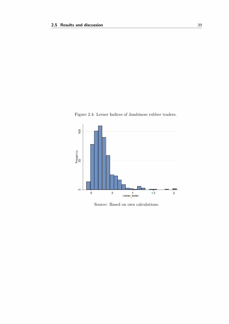
2.5 Results and discussion 39
Figure 2.4: Lerner Indices of Jambinese rubber traders.
Source: Based on own calculations.

40 Traders and Credit Constrained Farmers
Table 2.6: Determinants of market power that is exercised by traders.
Determinants Lerner Index
number traders karet -0.0339***(0.0001)
log house cost -0.0086(0.387)
providing farms -0.0013**(0.0344)
providing traders 0.0056***(0.0001)
pos in chain decimals 0.1310***(0.0001)
transmigrasi village -0.1190(0.494)
general remoteness 0.0041**(0.0313)
dist to closest auction market 0.0048***(0.0001)
households in village 0.0004***(0.0001)
no podes2008 data 0.4060**(0.0155)
agric area non rice -3.32e-06**(0.0466)
formal credit available -0.4400***(0.0001)
informal credit available -0.0701(0.541)
credit mio -0.0011*(0.0639)
quality credit adjusted -0.0062(0.144)
little information 0.1570***(0.0001)
discusses prices 0.1480***(0.000110)
price agreements -0.2480**(0.0115)
ethnic resp java -0.0100(0.915)
Constant -0.0026(0.996)
Observations 466R-squared 0.869
Standard errors in parenthesesTrader dummies not reported. Full results are available on demand.
*** p<0.01, ** p<0.05, * p<0.1

2.6 Conclusions 41
size than population size. One explanation for the positive relationship between
village size and market power could be that anonymity can be expected to be
greater in larger settlements, which reduces the general level of mutual trust and
fairness. Another factor that reduces the Lerner Index (i. e. increases competition)
is the proximity to an auction market. Also, the more remote the location of a
trader is, the more successful he or she is in exercising his or her market power.
Traders who buy from many other traders (and relatively fewer farmers) can be
considered to be in a relatively good bargaining position which is indicated by an
increasing Lerner Index. According to the data, the availability of at least one
formal credit institution reduces the market power of traders which supports the
arguments laid out in the theoretical part. However, it seems that farmers who
do get more credit from the traders are also the ones who receive better prices
compared to the ones without credits. The reason behind this is that farmers
taking relatively little credit receive a higher interest rate due to the fixed costs
of providing credit. In the context of this study, these fixed costs consist of the
time the trader invests to generate and continue personal ties with the debtor,
as well as the time spent observing him or her. While traders’ general access to
information is negatively related to their ability to exercise market power, the ones
who discuss the prices which they pay with other traders generate higher margins.
This is another indicator pointing towards collusion.
2.6 Conclusions
The results of this study indicate that agricultural traders in Indonesia, more specif-
ically the Jambinese rubber traders, possess monopsonistic market power. This
could be shown via an innovative approach that was enabled by an exceptional set
of data: we had access to detailed sales data on a single-transaction level. Such
data are at a much more disaggregated level than in any other examples in the lit-
erature. These data enabled the estimation of a revenue function, which was used
to directly calculate hypothetical rubber prices under the assumption of perfect
competition. The hypothetical prices were compared to the observed prices that
middlemen for rubber pay to their providers via calculating Lerner Indices. These
proved to be significantly different from zero – a clear indication of market power.
In a second stage, the Lerner Indices were regressed on different characteristics
of the market, of the traders and of the relationships between traders and their
providers. If local markets are smaller (less agricultural output, fewer traders),
the traders have more opportunities to exercise market power, as well as having
a more remote location. Improving infrastructure could reduce the influence of
42 Traders and Credit Constrained Farmers
‘remoteness’ on the functioning of the Jambinese rubber markets, as does the
establishment of auction markets in a larger number. Since the availability of
formal credit institutions is also negatively related to the exercise of market power,
the support of farmers through micro credit might also help.
If our explanation of the influence of village size on market power is correct (and
the verification of this certainly calls for further research), policy makers should
focus on measures improving trust and comradeship between villagers.


Chapter 3
Have Indonesian Rubber
Processors Formed a Cartel?
Analysis of Intertemporal
Marketing Margin
Manipulation
45
Have Indonesian Rubber Processors Formed a Cartel?
Analysis of Intertemporal Marketing Margin
Manipulation
Thomas Kopp1, Zulkifli Alamsyah2, Raja Sharah Fatricia2 and Bernhard
Brummer1
1Georg August University, Gottingen, Germany 2Jambi University, Jambi,
Indonesia
Abstract
In Indonesia the agricultural sector plays a key role for inclusive economic de-
velopment in rural areas. In the Jambi province, rubber is the most valuable
export crop produced by small scale agriculture. The observed concentration
in the crumb rubber processing industry raises concerns about the distribu-
tion of export earnings along the value chain. In this study we investigate the
price transmission between international prices and the factories’ purchasing
prices. We make use of the non-parametric estimation technique of penalized
splines in order to understand the error correction process without the need
for restrictive a priori assumptions. We then estimate an Auto-Regressive
Asymmetric Threshold Error Correction Model to find evidence for asymmet-
ric price transmission, and to quantify the extent of the threshold effect. In
a second step we calculate the rents that are redistributed. The analysis is
based on daily price information over a period of four years (2009-2012). Our
results suggest that factories transmit prices asymmetrically, which has sub-
stantial welfare implications: around three million U.S. Dollars are annually
redistributed from Jambinese farmers to factories.
3.1 Introduction
For Indonesia the agricultural sector is of great importance. In 2011 it contributed
15% to the GDP and employed 36% of the workforce.1 The most valuable export
1WorldBank World Development Indicators. Accessed March 2015, available at http:
//databank.worldbank.org.
46

3.1 Introduction 47
crop is natural rubber. With an annual output of three million metric tons, In-
donesia is the second largest producer of natural rubber in the world, accounting
for 27% of global production.2 More than 15 million people generate their main
income from rubber cultivation (Fathoni, 2009).
In the future, it is likely that the importance of rubber for Indonesia will increase
for two reasons. Firstly, the total demand for any kind of rubber will increase,
due to economic growth in the emerging economies; and secondly the ever-rising
price of crude oil will make synthetic rubber more expensive and thus increases the
demand for its substitute natural rubber.
Rubber is predominately produced on the islands of Sumatra and West Kalimantan.
They contribute 72% to the total production of the country (Arifin, 2005). The
province of Jambi (Sumatra) is one example of a province that depends crucially
on its agricultural sector. It also represents a typical rubber production area.
52% of the workforce is employed in the agricultural sector and 0.6 million ha
(out of 1.4 million ha) are dedicated to rubber production, of which 99.6% are
cultivated by smallholders (Regional Account and Statistical Analysis Division,
2012). Although Jambi is on average not an exceptionally poor province, the rural
population is still disadvantaged compared to the populations in other parts of
Indonesia. The average income is 17.5 million Indonesian Rupiah (1 600 USD)3
per year (Arifin, 2005; Regional Account and Statistical Analysis Division, 2012),
which is far below the national average of 26.8 million Rupiah (2 450 USD) per
year.4 Other development indicators show a similar picture, for example the life
expectancy at birth is 71 years in Jambi, compared to 76 years in Jakarta (Regional
Account and Statistical Analysis Division, 2012).
As rubber is predominantly cultivated by smallholders, rubber does have the po-
tential to be one key to economic and social development in rural areas, improving
the socio economic situation of millions. In total, 252 000 Jambinese households
(out of 619 000) depend on rubber cultivation (Regional Account and Statistical
Analysis Division, 2012). This means that roughly one million people in Jambi are
affected.
It follows that malfunctions in this market can have a tremendous effect on the
livelihoods of small scale farmers and their families if imperfections in the rubber
market are disadvantageous for this group. It should therefore be a primary policy
target to ensure that these markets function properly.
2FAO FAOSTAT. Accessed March 2015, available at http://faostat3.fao.org/home/E.3Exchange rate (December 2013) from Oanda Corporation.4WorldBank: WorldBank World Development Indicators. Accessed March 2015, available at
http://databank.worldbank.org.

48 Have Indonesian Rubber Processors Formed a Cartel?
However, this does not seem to be the case. The Jambinese rubber sector is char-
acterized by strong oligopsonistic market power. On the processing side we can
observe a strong concentration of the demand for the product of the farmers, as
there are only nine crumb rubber factories in Jambi, vis-a-vis 252 000 farmers.
These factories do not appear to be in tight competition, but are rather collaborat-
ing closely. All of them are organized in the association of the rubber processing
sector, Gapkindo. A report prepared for the development agency USAID by Per-
amune and Budiman (2007) found that Gapkindo is a very efficiently organized
and politically powerful lobbying-institution that represents the interests of rubber
processors and brokers. Its main target is ‘the development of rubber processing
industries’ and to ‘network among members’ (Peramune and Budiman, 2007, p. 32).
There are strong indications that some individual firms exploit their network to
behave in a way that resembles a classical cartel or oligopsony (ibid.). Within the
scope of this analysis it cannot clearly be distinguished between a cartel and an
oligopoly since the data required for a game theoretical approach or the determi-
nation of the cartel price (cost structures of the factories, demand structure) are
not available. The establishment of the link between the evidence for asymmetric
price transmission and the occurrence of market power is based on Meyer and von
Cramon-Taubadel (2004).
In order to shed light on the price formation process in the rubber value chain,
we are employing a price transmission approach. In particular we study the ver-
tical transmission between the output- and input prices of the five crumb rub-
ber factories in Jambi City from 01 January 2009 until 31 December 2012 via an
Asymmetric Threshold Error Correction Model (ATECM), as introduced by von
Cramon-Taubadel (1998). To specify the error correction model correctly and with-
out having to rely on a priori assumptions, we employ the non-parametric technique
of penalized splines before estimating a set of candidate parametric models and test
which one represents the data best, as suggested by Serra et al. (2006). In addition
to demonstrating the existence and extent of market power, we also quantify a part
of the resulting redistribution of welfare from the suppliers to the factories. These
welfare implications are shown to be substantial.
To the best of our knowledge, this is the first paper combining the approaches
of non-parametric and parametric estimation techniques of estimating asymmetric
price transmission processes with a welfare perspective to quantify the distribu-
tional consequences of this intertemporal marketing margin manipulation. The
dataset of daily prices on such a disaggregated and local level is unique.
The paper is organized as follows: section two provides the background of the
rubber market in the Jambi province and introduces the typical marketing chain

3.2 Background 49
for natural rubber originating from smallholder production in this area. In section
three the intuition behind asymmetric price transmission is discussed. Section four
is dedicated to the model development, and section five presents the statistical
results. The subsequent section six derives the resulting welfare implications before
section seven concludes.
3.2 Background
Rubber marketing in the Jambi Province
The Jambinese rubber sector is displayed in Figure 3.1.5 Most farmers sell to a
village trader who then has the choice between three different kinds of stakeholders
to sell to: a factory, a warehouse or another trader, for example on the district
level. This choice is influenced by various factors, including the remoteness of the
trader, her capital, access to credit and information, etc. (Sujarwo et al., 2014).
Figure 3.1: Marketing channels for rubber.
Source: author’s calculations, based on own survey data (2012) and Euler et al.(2012). The percentages indicate which marketing channel is employed and for howoften.
There are approximately 16 000 traders in the Jambi province and nine factories of
which five are located in the capital Jambi City (citealpRegionalAccountandSta-
tisticalAnalysisDivision2012 and own survey data, 2012).
5Farmers’ marketing channels do not add up to 100, because they sell a minor share on auctionmarkets (6%) where the buyer is unknown, as well as to farmers’ associations (1%). The missing13% of the district traders stem from the fact that they can also sell to another trader, which wasomitted from this graph.
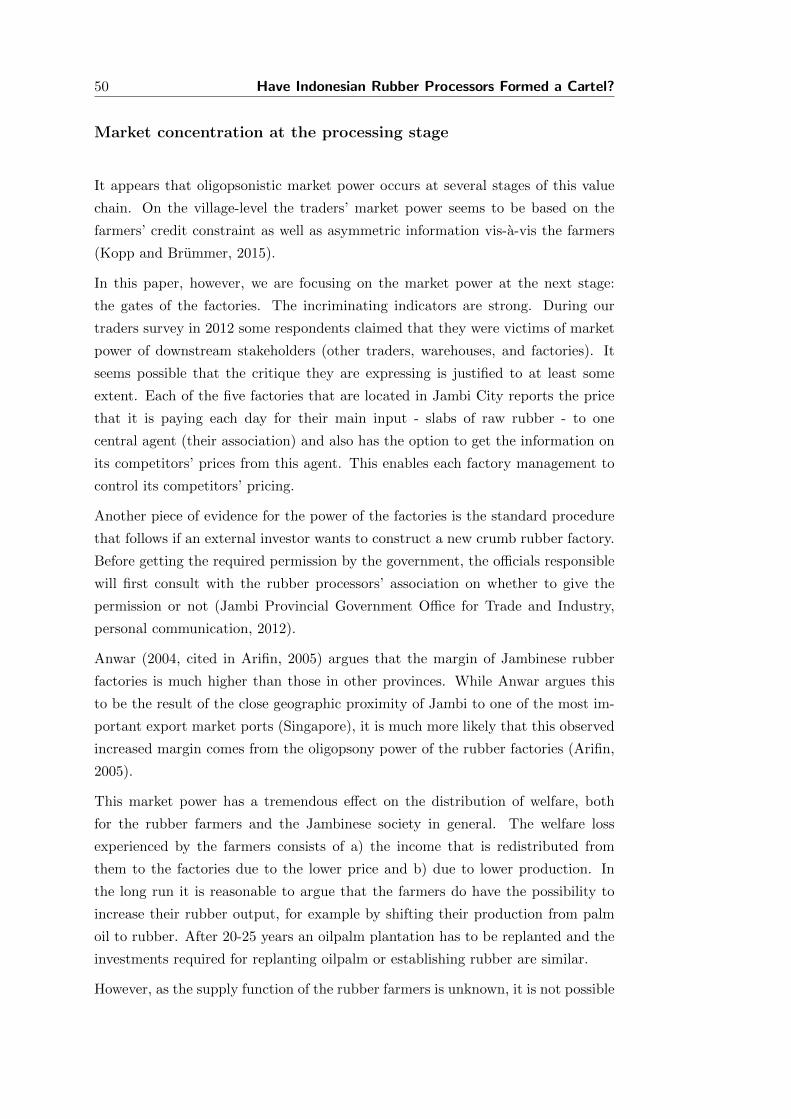
50 Have Indonesian Rubber Processors Formed a Cartel?
Market concentration at the processing stage
It appears that oligopsonistic market power occurs at several stages of this value
chain. On the village-level the traders’ market power seems to be based on the
farmers’ credit constraint as well as asymmetric information vis-a-vis the farmers
(Kopp and Brummer, 2015).
In this paper, however, we are focusing on the market power at the next stage:
the gates of the factories. The incriminating indicators are strong. During our
traders survey in 2012 some respondents claimed that they were victims of market
power of downstream stakeholders (other traders, warehouses, and factories). It
seems possible that the critique they are expressing is justified to at least some
extent. Each of the five factories that are located in Jambi City reports the price
that it is paying each day for their main input - slabs of raw rubber - to one
central agent (their association) and also has the option to get the information on
its competitors’ prices from this agent. This enables each factory management to
control its competitors’ pricing.
Another piece of evidence for the power of the factories is the standard procedure
that follows if an external investor wants to construct a new crumb rubber factory.
Before getting the required permission by the government, the officials responsible
will first consult with the rubber processors’ association on whether to give the
permission or not (Jambi Provincial Government Office for Trade and Industry,
personal communication, 2012).
Anwar (2004, cited in Arifin, 2005) argues that the margin of Jambinese rubber
factories is much higher than those in other provinces. While Anwar argues this
to be the result of the close geographic proximity of Jambi to one of the most im-
portant export market ports (Singapore), it is much more likely that this observed
increased margin comes from the oligopsony power of the rubber factories (Arifin,
2005).
This market power has a tremendous effect on the distribution of welfare, both
for the rubber farmers and the Jambinese society in general. The welfare loss
experienced by the farmers consists of a) the income that is redistributed from
them to the factories due to the lower price and b) due to lower production. In
the long run it is reasonable to argue that the farmers do have the possibility to
increase their rubber output, for example by shifting their production from palm
oil to rubber. After 20-25 years an oilpalm plantation has to be replanted and the
investments required for replanting oilpalm or establishing rubber are similar.
However, as the supply function of the rubber farmers is unknown, it is not possible

3.3 Methodology 51
to derive how much the supplied quantity and thus the total welfare loss would be in
the case of a general improvement of the price level. Therefore we will concentrate
on the farmers’ welfare loss due to the redistribution based on a below competitive
market price in times of price hikes. We are going to show that this oligopsonistic
market power is exercised and how large the welfare loss to the farmers is, that
results from intertemporal marketing margin manipulation.
3.3 Methodology
One way of finding empirical evidence for the existence of market power is by
testing for a non-constant transmission of price changes (Kinnucan and Forker,
1987; McCorriston et al., 2001; Meyer and von Cramon-Taubadel, 2004). We are
aware that the literature of New Empirical Industrial Organization provides with
structural models a more direct approach to indications of market power (Bresna-
han, 1982). However, these approaches require detailed information on the firms’
demand and supply structures, which is data on a level of detail that we do not
have access to. The asymmetry that we are discussing here implies that positive
changes of an agent’s selling price are passed on to her provider at a lower speed
than negative price changes. This means that when the agent’s margin increases
– that is in times of international price hikes – the buying price is corrected less
rapidly than when the margin decreases.6
The assumption behind the asymmetric price transmission between the interna-
tional rubber price and the Jambinese price for raw rubber is that the factories
are price takers at the international market. While Indonesia as a whole can be
assumed to have an influence on international rubber prices, this is unlikely to be
true for the five Jambinese factories under consideration. At the domestic market,
however, it can be assumed that they are price setters. Both these assumptions
are going to be tested. One can therefore understand the shocks that arise in the
first one as exogenous and the ones in the latter as reactions to that shock. In
Figure 3.2, the two lines represent the input- and output-prices. The margin of the
factory is the squared area. Negative shocks are transmitted faster than positive
ones, which means that in the case of a negative shock the margin of the processor
stays constant, while after a positive shock the margin increases (striped area).
The assumption behind the asymmetric price transmission between the interna-
tional rubber price and the Jambinese price for raw rubber is that the factories
6If asymmetries in the short-run dynamics occur (not only in the adjustment parameter) itwould also be interesting to analyse these dynamics via impulse response functions. As we willsee however, there are no asymmetries in the short-run dynamics, so the generation of impulseresponse functions would not increase the quality of information.
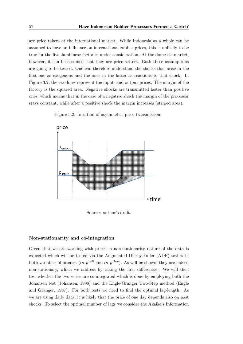
52 Have Indonesian Rubber Processors Formed a Cartel?
are price takers at the international market. While Indonesia as a whole can be
assumed to have an influence on international rubber prices, this is unlikely to be
true for the five Jambinese factories under consideration. At the domestic market,
however, it can be assumed that they are price setters. Both these assumptions
are going to be tested. One can therefore understand the shocks that arise in the
first one as exogenous and the ones in the latter as reactions to that shock. In
Figure 3.2, the two lines represent the input- and output-prices. The margin of the
factory is the squared area. Negative shocks are transmitted faster than positive
ones, which means that in the case of a negative shock the margin of the processor
stays constant, while after a positive shock the margin increases (striped area).
Figure 3.2: Intuition of asymmetric price transmission.
Source: author’s draft.
Non-stationarity and co-integration
Given that we are working with prices, a non-stationarity nature of the data is
expected which will be tested via the Augmented Dickey-Fuller (ADF) test with
both variables of interest (ln pSell and ln pBuy). As will be shown, they are indeed
non-stationary, which we address by taking the first differences. We will then
test whether the two series are co-integrated which is done by employing both the
Johansen test (Johansen, 1998) and the Engle-Granger Two-Step method (Engle
and Granger, 1987). For both tests we need to find the optimal lag-length. As
we are using daily data, it is likely that the price of one day depends also on past
shocks. To select the optimal number of lags we consider the Akaike’s Information

3.3 Methodology 53
Criterion (AIC), Schwarz’s Bayesian information criterion (SBIC), and Hannan
and Quinn information criterion (HQIC).
Error correction model
We assume a multiplicative mark-up model. The intuition behind using a mul-
tiplicative instead of an additive model is that the margin is assumed to be a
percentage markup. This has been concluded from qualitative interviews with
representatives of the rubber factories. We have tested both approaches, and the
results confirmed that taking the logarithm represents the data better. pBuyt refers
to the buying price at time t and pSellt to the selling price. The long-run (‘co-
integrating’) relationship in its logarithmic form is given by
ln pBuyt = β0 + β1 ln pSellt + ε (3.1)
which we estimate with the Johansen method. The reason for doing so (despite
our general approach of the Engle-Granger two-step method) is that the Johansen
approach delivers better results when estimating the co-integrating relationship
(Gonzalo, 1994). From the residuals of this relation we can generate the error
correction term (ect) which is defined as follows:
ectt := ln pBuyt − β0 − β1 ln pSellt (3.2)
In the case of a positive price shock on the international level (i. e. a positive
deviation from the long-run equilibrium in which the factories’ margin increases)
the ect will be < 0 and if the price is shocked negatively, the ect is > 0. The error
correcting process (symmetric case) is expressed as
∆ ln pBuyt = ξ0 + α ectt−1 +M∑ω=1
(γω∆ ln pBuyt−ω + λω∆ ln pSellt−ω
)+ ε (3.3)
M is the number of lags, ξ0 a constant, and γω and λω the coefficients of short-run
dynamics. ε represents an error term. Figure 3.3 (continuous line) illustrates the
error correcting process by graphing the ect from the previous period against the
change of the buying price in the current period. In the 2nd quadrant the correction
of positive price shocks is represented while the correction of negative shocks can
be seen in the 4th quadrant.
For the thoughts laid out in the theoretical section above, the model is extended
to a threshold error correction process, which is the generalization of a simple

54 Have Indonesian Rubber Processors Formed a Cartel?
asymmetric adjustment. The existence of any threshold is tested for with a SupLM
test as suggested by Hansen and Seo (2002). Based on model (3) the ect is split up
into N regimes by N − 1 thresholds, which are located at Ψλ for λ ∈ [1, . . . , N − 1]
and ectςt := ectt if Ψς−1 < ectt ≤ Ψς for ς ∈ [1, . . . , N ]:
∆ ln pBuyt = ξ0 +N∑ς=1
αςectςt−1 +
M∑ω=1
(γω∆ ln pBuyt−ω + λω∆ ln pSellt−ω
)+ ε (3.4)
For an ‘asymmetric’ process, which is the simplest form of a threshold error cor-
rection (N=2 and Ψ1=0), the error correction is displayed in Figure 3.3 (dotted
line).
Figure 3.3: Symmetric error correction (continuous line) and asymmetric errorcorrection (dotted line).
Source: author’s draft.
Non-parametric estimation
Most authors in the literature on threshold error correction models use a parametric
estimation technique (Hansen and Seo, 2002, Lloyd et al., 2006, and Ihle et al.,
2012). The drawback of this procedure is that one has to make certain a priori
assumptions for specifying the model, such as the number of thresholds. In order
to overcome this limitation, we employ a non-parametric approximation. While
using non-parametric estimation techniques to detect unknown relationships is a
widely used technique in the statistical and financial literature (Krivobokova et al.,
2010; Escribano, 2004), in the agricultural economics literature this has not been

3.3 Methodology 55
employed a lot. An exception is the work by Serra et al. (2006) who use a local
polynomial fitting approach in order to understand the error correction process
without the need for restrictive a priori assumptions. Contrary to that, we are
working with penalized splines (Eilers and Marx, 1996). Regression splines consist
of the sum of a number of polynomial functions. The spline is fitted to match the
data by giving each of these functions an individual shape. Penalizing the splines
refers to the method of including a penalty-term, which smoothes the spline by
penalizing excessive zigzagging (i. e. big differences between neighboring values) of
the spline (Wood, 2003).
Candidate models for parametric estimation
In order to get to know the exact slope-coefficients which are necessary for cal-
culating the distributional effects, we will continue with a parametric regression
approach, based on the insights from the non-paramethric methods. Several ap-
proaches are employed to model the error correction process before the model that
represents the data best will be chosen via a testing procedure described below.
To start with, we estimate a simple linear error correction model (M1) which cor-
responds to the model described in equation 3.3. The second model (M2) is an
asymmetric error correction model which corresponds to equation 3.4 with the
specifications N=2 and Ψ1=0. For the third model (M3) we assume a one-threshold
model with no restriction on the location of the threshold. The intuition of model
three (M3) is that the price gets corrected quickly during price drops (regime 3)
and moderate hikes (regime 2) when the factories generate a normal margin. In
times of large price increases (regime 1) however, the prices get corrected much
slower: the factories generate a greater margin. M3 corresponds to equation 3.4
with N=2 and an unknown value of Ψ1.7.
The exact location of this threshold can be found via a grid search approach. We
test each possible value of the ect as the threshold value Ψ1, estimate the model
and save the log-likelihood value. We then select the model with the highest log-
likelihood.
Threshold determination and model choice
We find the threshold of model M3 via the grid search following the method laid
out above. At the same time, no assumptions have been made about the location
of the threshold.
7It was also experimented with a smooth-transition type of model as employed by Hassounehet al. (2012). The results did not show statistical significance, but can be made available ondemand.

56 Have Indonesian Rubber Processors Formed a Cartel?
After estimating the different models described (M1-M3), we will test which of
them represents the data best. As we compare models with different specifications
concerning the number of regimes (one and two), we rely on an information criterion
again. We employ the AIC which is in this case superior to other information
criteria as laid out by Burnham and Anderson (2002).
Distributional effects
The quantification of the distributional effects stemming from asymmetric price
transmission is based on the forgone profit for smallholders due to slower price
transmission in times of tremendous price hikes, compared to a baseline scenario of
the fastest adjustment possible which is assumed to be the adjustment that occurs
in times of price decreases (see Figure 3.4). As discussed above, we do not focus
on the total welfare effect because the price elasticities of the supply and demand
are unknown. The part of the welfare effect which stems from the intertemporal
marketing margin manipulation is calculated as the difference between the price
that is theoretically possible in times of price hikes and the price that is actually
paid, multiplied by the quantity. The generation of impulse response functions
would not increase the quality of information, since the short-run dynamics were
not proven to be asymmetric.
Figure 3.4: Welfare effect during adjustment process after shock at t=0
(a) time = t+1 (b) time= t+10
Source: author’s draft.
In order to quantify the effect that the intertemporal marketing margin manip-
ulation had on all Jambinese farmers, we calculate the differences between two
hypothetical scenarios of the local price development after 14 periods (the time af-
ter which a farmer sells his/her produce is around two weeks) following each shock
to the global price during 2009-2012. The two scenarios differ in the assumed
3.4 Data 57
adjustment parameter, following the results from the asymmetric error correction
model.
We start with the following equation
ln pBuyt = ln pBuyt−1 + ∆ ln pBuyt + ε (3.5)
in which we substitute ∆ ln pBuyt from a simplified version (without lagged prices)8
of equation 3.3 and then ectt from equation 3.2 in order to calculate the adjusted
price after one period:9
ln pBuyt = ln pBuyt−1 + α(
ln pBuyt−1 − β0 − β1 ln pSellt−1
)+ ε (3.6)
Iterating this procedure 14 times generates the price after 14 periods after the
shock in period 1. In the computation we omit the error term, assuming it to be
zero. The difference pdiff between the two scenarios is given as
pdiff = exp
(ln p
Buy(α+)t+14
)− exp
(ln p
Buy(α−)t+14
)(3.7)
The total redistribution (RED) based on intertemporal marketing margin manip-
ulation is then the sum of all price differences, multiplied by the quantity sold at
time t+ 14:
RED =
T∑t=1
(pdifft qt+14
)(3.8)
3.4 Data
The daily buying prices from the five factories in Jambi City were provided by
Gapkindo. There is one price for each factory available for each day from 1 January
2009 until 31 December 2012, except for Sundays and public holidays. Out of these
five series, an unweighted average for the Jambi-buying price was generated. The
selling prices were drawn from PT. Kharisma (2013), a marketing company located
in Jakarta. These prices represent the average results of the auctioning of Standard
Indonesian Rubber (SIR20) on each day when rubber was sold (four or five days per
week, except for two weeks of Christmas holidays and two weeks during Ramadan).
8We can make this simplification of equation 3.3 since the short-run dynamics are not asym-metric.
9The adjustment of pSell to pBuy is close to zero, since pSell was shown above to be clearlythe leading price, and not reacting to pBuy)

58 Have Indonesian Rubber Processors Formed a Cartel?
In combination, this gives us 706 days for which we have both selling and buying
prices. The price series are graphed in Figure 3.5.
Figure 3.5: Time series of buying and selling prices.
Source: author’s production. Values are the logarithm of the prices in IndonesianRupiah. 1.00 USD = 10.93 Indonesian Rupiah (December, 2013). The green barindicates the existence of data, so the holes in the green bar represent days withoutdata. In the graph, the last point before a gap was connected with the first oneafter it.
3.5 Results
Non-stationarity and co-integrating relationship
The initial suspicion could be confirmed. The series are indeed both non-stationary
(the H0 of non-stationarity cannot be rejected at a confidence level of 10%). To
avoid the problem of spurious regressions, we take the first differences. As the
results of the ADF test show (H0 can be rejected at a 1% confidence level), this
solves the problem. The SBIC suggests a lag-length of the order two, the HQIC
three lags, and the AIC opts for four lags. Following Ivanov and Kilian (2005),
who suggest to trust the AIC in situations of large sample sizes (>250) and data
of relatively high frequency (>weekly), we use four lags. The second reason for
choosing the lag order suggested by the AIC is the danger of biasing the results by
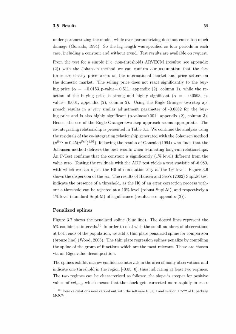
3.5 Results 59
under-parametrizing the model, while over-parametrizing does not cause too much
damage (Gonzalo, 1994). So the lag length was specified as four periods in each
case, including a constant and without trend. Test results are available on request.
From the test for a simple (i. e. non-threshold) ARVECM (results: see appendix
(2)) with the Johansen method we can confirm our assumption that the fac-
tories are clearly price-takers on the international market and price setters on
the domestic market. The selling price does not react significantly to the buy-
ing price (α = −0.0153, p-value= 0.511, appendix (2), column 1), while the re-
action of the buying price is strong and highly significant (α = −0.0593, p-
value= 0.001, appendix (2), column 2). Using the Engle-Granger two-step ap-
proach results in a very similar adjustment parameter of -0.0582 for the buy-
ing price and is also highly significant (p-value=0.001: appendix (2), column 3).
Hence, the use of the Engle-Granger two-step approach seems appropriate. The
co-integrating relationship is presented in Table 3.1. We continue the analysis using
the residuals of the co-integrating relationship generated with the Johansen method
(pBuy = 0.45(pSell)1.07), following the results of Gonzalo (1994) who finds that the
Johansen method delivers the best results when estimating long-run relationships.
An F-Test confirms that the constant is significantly (1% level) different from the
value zero. Testing the residuals with the ADF test yields a test statistic of -6.980,
with which we can reject the H0 of non-stationarity at the 1% level. Figure 3.6
shows the dispersion of the ect. The results of Hansen and Seo’s (2002) SupLM test
indicate the presence of a threshold, as the H0 of an error correction process with-
out a threshold can be rejected at a 10% level (robust SupLM), and respectively a
1% level (standard SupLM) of significance (results: see appendix (2)).
Penalized splines
Figure 3.7 shows the penalized spline (blue line). The dotted lines represent the
5% confidence intervals.10 In order to deal with the small numbers of observations
at both ends of the population, we add a thin plate penalized spline for comparison
(bronze line) (Wood, 2003). The thin plate regression splines penalize by compiling
the spline of the group of functions which are the most relevant. These are chosen
via an Eigenvalue decomposition.
The splines exhibit narrow confidence intervals in the area of many observations and
indicate one threshold in the region [-0.05; 0], thus indicating at least two regimes.
The two regimes can be characterized as follows: the slope is steeper for positive
values of ectt−1, which means that the shock gets corrected more rapidly in cases
10These calculations were carried out with the software R 3.0.1 and version 1.7-22 of R packageMGCV.

60 Have Indonesian Rubber Processors Formed a Cartel?
Figure 3.6: Distribution of ect values.
Source: author’s production. The extreme values at the left end of the distributionare not outliers, but plausible values for the ect. They all occurred during onetremendous price hike from 17.-24. March 2011.
Table 3.1: Estimates of long-run relation.
ln pBuy OLS Johansen
ln pSell 1.067*** 1.067***(0.0071) (0.0186)
Constant -0.811*** -0.800(0.0723)
Observations 706 702R-squared 0.982
Standard errors in parentheses*** p<0.01, ** p<0.05, * p<0.1
Since the VEC is not linear, it does not report t-statistics. The Johansen resultshave four observations less, because they include lags, while the first step of theEngle-Granger method does not require the inclusion of lags.
of negative price-shocks than in the case of positive price-shocks. While in the area
[-0.1; 0] the splines are robust to changes in their specification,11 the confidence
intervals widen substantially at the rather extreme values in ]−∞;−0.1[∪]0.1;∞[,
which is caused by the small number of observations in these areas.
11Available on request.

3.5 Results 61
Figure 3.7: Penalized splines.
Source: author’s production.
Model choice
Table 3.2 presents the AIC values of the models M1-M3. Following this crite-
rion, M3 represents the data best. Executing an F-Test indicates that the two
slope-coefficients of Model 3 are different from each other with a significance of
6.58%. The following discussion is therefore based on the two-regime model with
one threshold at -0.0383844 (M3).
Table 3.2: Results of Akaike Information Critereon.
Model ln(L) k AIC Rank
M1 2223.7814 10 -4427.5628 3M2 2224.8331 11 -4427.6662 2M3 2226.7141 11 -4431.4282 1
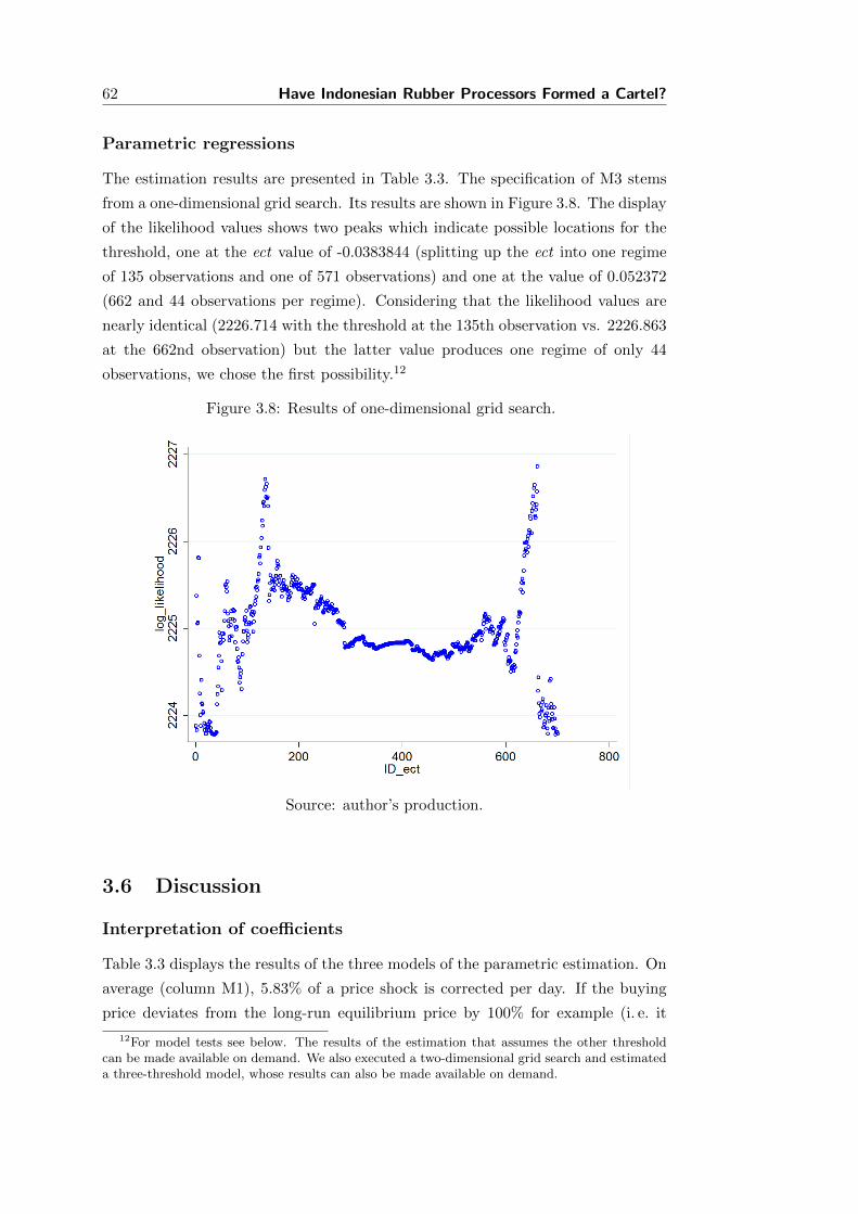
62 Have Indonesian Rubber Processors Formed a Cartel?
Parametric regressions
The estimation results are presented in Table 3.3. The specification of M3 stems
from a one-dimensional grid search. Its results are shown in Figure 3.8. The display
of the likelihood values shows two peaks which indicate possible locations for the
threshold, one at the ect value of -0.0383844 (splitting up the ect into one regime
of 135 observations and one of 571 observations) and one at the value of 0.052372
(662 and 44 observations per regime). Considering that the likelihood values are
nearly identical (2226.714 with the threshold at the 135th observation vs. 2226.863
at the 662nd observation) but the latter value produces one regime of only 44
observations, we chose the first possibility.12
Figure 3.8: Results of one-dimensional grid search.
Source: author’s production.
3.6 Discussion
Interpretation of coefficients
Table 3.3 displays the results of the three models of the parametric estimation. On
average (column M1), 5.83% of a price shock is corrected per day. If the buying
price deviates from the long-run equilibrium price by 100% for example (i. e. it
12For model tests see below. The results of the estimation that assumes the other thresholdcan be made available on demand. We also executed a two-dimensional grid search and estimateda three-threshold model, whose results can also be made available on demand.
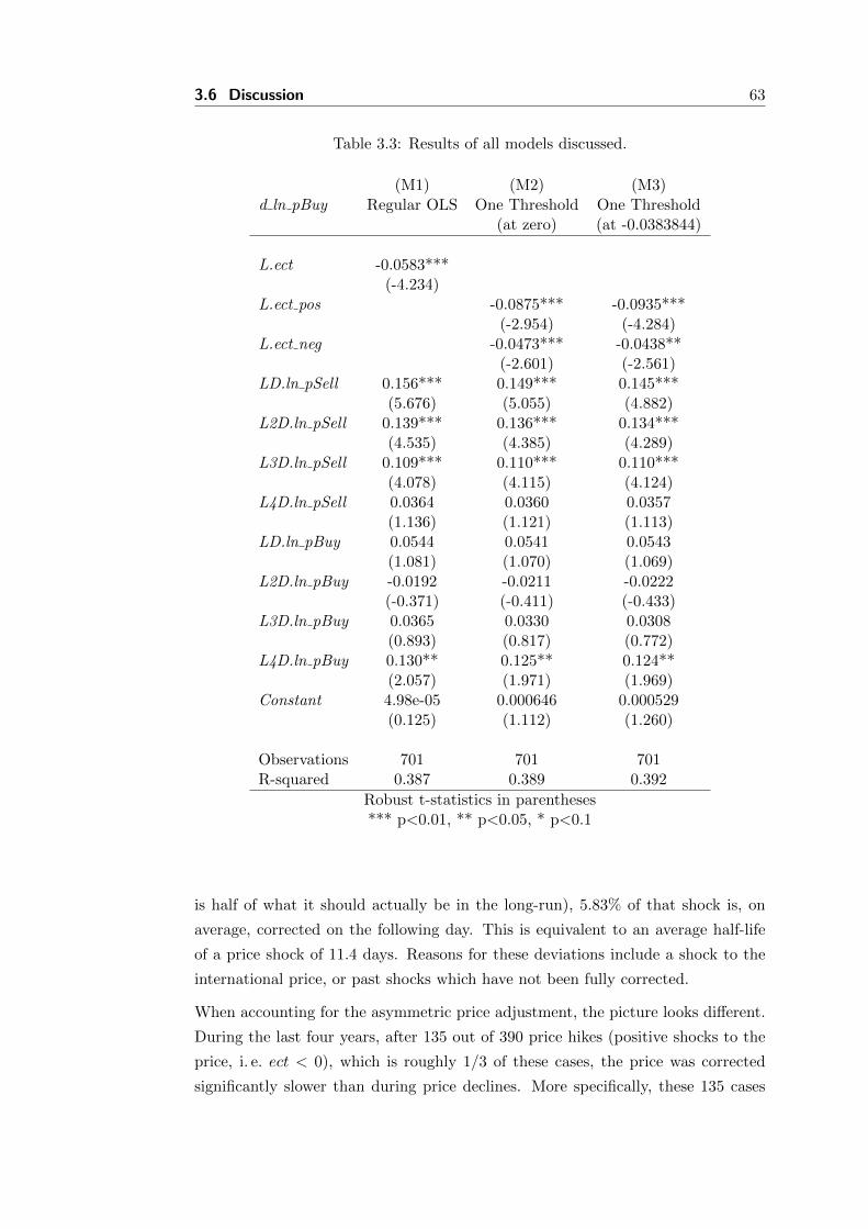
3.6 Discussion 63
Table 3.3: Results of all models discussed.
(M1) (M2) (M3)d ln pBuy Regular OLS One Threshold One Threshold
(at zero) (at -0.0383844)
L.ect -0.0583***(-4.234)
L.ect pos -0.0875*** -0.0935***(-2.954) (-4.284)
L.ect neg -0.0473*** -0.0438**(-2.601) (-2.561)
LD.ln pSell 0.156*** 0.149*** 0.145***(5.676) (5.055) (4.882)
L2D.ln pSell 0.139*** 0.136*** 0.134***(4.535) (4.385) (4.289)
L3D.ln pSell 0.109*** 0.110*** 0.110***(4.078) (4.115) (4.124)
L4D.ln pSell 0.0364 0.0360 0.0357(1.136) (1.121) (1.113)
LD.ln pBuy 0.0544 0.0541 0.0543(1.081) (1.070) (1.069)
L2D.ln pBuy -0.0192 -0.0211 -0.0222(-0.371) (-0.411) (-0.433)
L3D.ln pBuy 0.0365 0.0330 0.0308(0.893) (0.817) (0.772)
L4D.ln pBuy 0.130** 0.125** 0.124**(2.057) (1.971) (1.969)
Constant 4.98e-05 0.000646 0.000529(0.125) (1.112) (1.260)
Observations 701 701 701R-squared 0.387 0.389 0.392
Robust t-statistics in parentheses*** p<0.01, ** p<0.05, * p<0.1
is half of what it should actually be in the long-run), 5.83% of that shock is, on
average, corrected on the following day. This is equivalent to an average half-life
of a price shock of 11.4 days. Reasons for these deviations include a shock to the
international price, or past shocks which have not been fully corrected.
When accounting for the asymmetric price adjustment, the picture looks different.
During the last four years, after 135 out of 390 price hikes (positive shocks to the
price, i. e. ect < 0), which is roughly 1/3 of these cases, the price was corrected
significantly slower than during price declines. More specifically, these 135 cases

64 Have Indonesian Rubber Processors Formed a Cartel?
were at times of extreme price hikes, i. e. ect < −0.0383844. It takes 16.5 days
to correct half of a strong positive price change and only 7.5 days in the case of
a negative or small positive shock (see Figure 3.9. The simulations are based on
equations 3.6 and 3.7, see below). The sign of the threshold value is counterintuitive
(negative ects refer to positive price changes) because the ect in the analysis was
defined as the long-run equilibrium price minus the actual price in that period. This
means, more plainly, that when the international price sinks, the factories’ buying
prices adjust twice as fast as when the international price rises strongly. The time
needed to correct 99% of a shock is 49 days in the case of a negative shock and 107
days in the case of a strong positive shock. The lagged values of pSellt are positive
and significant while the lags of pBuyt are insignificant which supports the results
from the Johansen test above that pSellt is the leading price.
Figure 3.9: Correction of shocks over time.
Source: author’s calculations. In Indonesian Rupiah; 1.00 USD = 10.93 IndonesianRupiah.
There are two reasons explaining why the price shocks are not transmitted in an
instant (9.4% per period is a very quick error correction, considering that we are
working with daily data). Firstly, technical reasons in the factories are an issue,
such as the communication between the selling and buying departments. The
second reason is more of a methodological issue. For the analysis, the average
of the prices of five crumb rubber factories was generated. Since changing their
prices identically would be too much of an obvious indication of collusion, there
are always small differences between the five prices. These small differences impact

3.6 Discussion 65
the average in a way that leads to an apparent short delay in the transmission time
that is the average between the firms.
Market power or not?
As asymmetries in price adjustments can be the result of different kinds of pro-
cesses, other than market power (von Cramon-Taubadel, 1998), this kind of anal-
ysis cannot provide a definite ’proof’ of market power. Meyer and von Cramon-
Taubadel (2004) show that asymmetric price transmission (APT) is not necessarily
caused by market power. In their literature review, they present an overview of
reasons for asymmetric price transmission other than market power, arguing that
the proof of asymmetric price transmission is not necessarily equivalent to a proof
of market power. For the case of our study however, all these alternative explana-
tions that can lead to APT can be ruled out, leading us to the conclusion that the
APT observed in the rubber processing sector in Jambi is indeed caused by market
power, based on cartelistic or oligopsonistic behavior.
a) ‘Menu costs’ or the costs associated with changing the price: the prices that the
factories are paying to their suppliers are changing every single day. There is no
reason to believe that the costs of changing the price depend on the direction
of the price change.
b) Fixed costs forcing a firm to operate close to its production capacity: as the
agricultural input (the slabs of coagulated rubber) is extremely durable; the
factories always have a stock available that is big enough to keep the factory
running for more than a week.
c) Perishability generates an incentive to sell the product quickly: processed crumb
rubber is not perishable.
d) A strong inflation in times of rising prices leads to data that exhibit asymmetry:
while the inflation of the Indonesian Rupiah is greater than that of the U.S.
Dollar, it is not great enough to have any impact on a daily basis which is the
horizon of our data.
e) Policy interventions, price support, etc. can also lead to asymmetric price trans-
mission, but has not occurred in Jambi (or on a national level in Indonesia)
during the timeframe under consideration. Neither were new factories built or
a new national/provincial government elected. The other input prices have also
stayed constant (energy has been subsidized at a constant level, and the mini-
mum wage did not change during the time of analysis). Hassouneh et al. (2010)
suggest searching for a regime-switch which we do not find.

66 Have Indonesian Rubber Processors Formed a Cartel?
f) Processing time: though a delayed reaction (caused by processing time) in com-
bination with high inflation can show misleading signs of APT, this does not
apply here because of two reasons: 1.) While it is true that inflation is high in
Indonesia (4.3% in 2012),13 we are working with daily data. During the typical
reaction times the price hike due to inflation is close to zero. 2.) Besides that,
we are observing a potentially monopsonistic setting, implying that the shock
that hits the leading (selling) price occurs after the processing. If factories who
set their buying price (and take their selling price) would want to set the buy-
ing price according to what they receive for that specific load of rubber after
processing, they would have to anticipate the price after the processing already
at the time of purchasing. This would be impossible.
g) Non-cooperative game: there are cases where it looks like price-fixing has hap-
pened, while in fact there is no outspoken agreement. It occurs in situations in
which firms possess a credible threat of punishing another firm which deviates
from the cartel-solution (Perloff et al., 2007). However, only rarely could it be
argued that these companies would have an agreement that is not the subject
of debate, especially given the fact that in all other respects they are such close
companions. Besides, even if there is indeed no explicit agreement on pricing,
the oligopsony-hypothesis would still hold.
An explanation why cartels adjust (increase) their buying prices at all – i. e. why
they do not always pay a low price to the farmers – is that even cartels face
restrictions concerning their price setting. There is always one margin that cannot
be exceeded without risking government interference. This is the margin that is
realized in times of constant or falling prices but secretly increased when the prices
rise.
Distributional consequences
The 252 000 Jambinese rubber producing smallholders produce 281 000 tons of
rubber per year on average (Regional Account and Statistical Analysis Division,
2012) and we assume them to sell, on average, the same amount every day at which
they sell. Entering all numbers into Equations 3.6 to 3.8 yields a forgone revenue
of 31.7 billion IDR (2.9 million USD) for the Jambinese rubber farmers in times
of rising prices in every year. This is only the amount that is redistributed from
farmers all over Jambi to the factories, due to the asymmetric price transmission
of the factories. The total welfare loss due to the below free-market prices can be
13Inflation in 2009: 4.8%, 2010: 5.1%, 2011: 5.4%. All from World Bank Database, 2015,dataset ‘Inflation, consumer prices (annual %).

3.7 Conclusions 67
assumed to be substantial, too. For a single farmer, this amount represents 2.25%
of his or her annual revenue. Considering that around 32% of the revenue turns
into profit (calculation based on Euler et al., 2012), the calculation of the forgone
profit is based on the following: profit π is equal to rs with r being the revenue,
and s the profit share of the revenue (32%). π = r − c with c representing the
costs. The possible increased revenue (if the price transmission was symmetrical)
r′ is equal to r(1 + x) with x being the percentage share of the possible increase
of the revenue (2.25%). Then π′ = r′ − c. The potential increase of profit can be
calculated as
(π′ − π
)/π = (r (1 + x)− c− (r + c)) / (rs) (3.9)
Increasing the revenue by 2.25% would have lead to an increased profit of 7.03%.
So effectively each farmer could have generated 6.97% more profit when the prices
were increasing by more than the threshold value.
3.7 Conclusions
The indications that the five rubber processing businesses in Jambi City, Sumatra
possess over proportional market power and use it to rig the prices which they
are paying to their suppliers are strong. In this paper we found evidence for an
asymmetric transmission of prices, which has led to a great redistribution of revenue
from the farmers to the processors during the four years of observation. Compared
to a non-monopsonistic market situation, the farmers have missed out on an income
from rubber production of 7%. The net welfare loss that has been generated in
the process could not be quantified in this analysis (due to missing information on
the price elasticities on the supply and demand sides), but can be assumed to be
substantial. It is likely that these kinds of processes occur all over Indonesia.
The group has achieved its advantage by correcting price changes on the inter-
national market (where its members act as price takers) asymmetrically. If the
international price drops, the buying price decreases much quicker than it adjusts
in times of great price hikes. All alternative explanations for asymmetric price
transmission - other than market power - could be ruled out for the rubber pro-
cessing sector in Jambi. Risk managing strategies would lead to a generally lower
price level, but not to a different reaction depending on the direction of price
changes.
One policy recommendation that could be drawn from our results is to involve all
stakeholders (including representatives of farmers) in the consultations before the

68 Have Indonesian Rubber Processors Formed a Cartel?
decision on granting permits for the construction of a new crumb rubber factory. If
more factories were competing for the input of raw rubber, the general price level
would be expected to increase.
Another issue that has been touched upon only briefly is the behavior between
the Jambinese rubber processors. It would be interesting to know if there is a
rather random selection of the stakeholder who applies price changes first, or one
clear Stackelberg leader determining the price with others who are following. With
this sort of game-theoretical approach one would be able to get an even more
detailed picture of the roles of the different stakeholders within the cartel, and the
functioning of it as a whole. This calls for research at a more disaggregated level.


Chapter 4
Preference Erosion - the Case
of Everything But Arms and
Sugar
71
Preference Erosion – the Case of Everything But Arms
and Sugar
Thomas Kopp1, Soren Prehn2 and Bernhard Brummer1
1Georg August University, Gottingen, Germany, 2Leibniz Institute of
Agricultural Development in Transition Economies, Halle (Saale), Germany
Abstract
While the European Union’s Everything But Arms (EBA) agreement has
granted unlimited preferential access to the European market for the Least De-
veloped Countries (LDCs) since 2001, the sugar sector has been exempted for
the first years. Only from 2009 on, the LDCs were entitled to export an unlim-
ited amount of sugar to the EU, receiving the intervention price. The expected
increase in sugar imports led the EU to substantially reduce the intervention
price, besides other measures. This caused a disadvantage for countries which
had been granted preferential access to the European market already: the
African, Caribbean, and Pacific (ACP) countries. Our paper quantifies this
erosion of preferences, employing a gravity framework. In terms of method-
ology we are addressing two fundamental problems well known in the gravity
literature. The occurrence of excess zeros in the dependent variable of such
disaggregated data is tackled with the employment of the scale-independent
Negative Binomial Quasi Generalised Pseudo Maximum Likelihood estimator.
The problem of identification is addressed by modeling the policy change with
the continuous Preference Margin instead of using dummy variables. We find
that preference erosion did occur. The ACP countries were indeed negatively
affected by the consequences following the introduction of the EBA.
Acknowledgments: We thank Maria Cipollina, Valentina Raimondi, and Luca
Salvatici for generously sharing working paper versions of upcoming papers.
72

4.1 Introduction 73
4.1 Introduction
The European Union’s Everything But Arms (EBA) agreement was designed to
make the poorest countries better off by granting them preferential access to the
common European market. But this noble goal might be overshadowed by some
unwanted by-effects for other countries. In this work we are taking a close look
at a potentially important phenomenon: preference erosion (PE), exemplified with
the case of sugar.
The European Union (EU) sugar market used to be regulated and strongly pro-
tected. It accounted for around two thirds of all protection that concerns trade
between the EU and less developed countries (Conforti et al., 2007). African,
Caribbean, and Pacific (ACP) countries have had preferential access to this pro-
tected market. But due to commitments following the negotiations of the World
Trade Organization’s Uruguay Round, as well as a lost panel against three big
sugar producing countries, there was a lot of pressure on the European Common
Market Organization (CMO) for sugar in the midst of the last decade to reduce
its subsidized sugar exports. In 2004 the WTO found that the EU were guilty of
subsidizing more sugar exports than it had committed itself to for two reasons: first
because the sugar that is supposedly exported without subsidies in fact enjoys an
indirect cross-subsidization1 via the sugar which is directly subsidized and secondly
it was found that the EU’s interpretation of one footnote of the agreement (con-
cerning exports equivalent to the size of the ACP-imports) was wrong (Hoekman
and Howse, 2008). Besides, the preferential agreements with the ACP countries
do not conform to WTO law in general. On one hand granting preferential ac-
cess to Least Developed Countries2 (LDCs) is explicitly allowed but it is forbidden
to discriminate within the group of all developing countries. Within the group of
ACP countries however, there is a growing number of countries which are not ’least
developed’. In order to comply, the ACP agreements had to be transformed into
Regional Trade Agreements (RTAs), which – again due to WTO law – must be
reciprocal.
In order to keep giving trade advantages to the poorest countries on earth and
conforming to WTO regulations, the Everything But Arms (EBA) agreement has
been introduced in 2001 which gives preferential access to the group of the Least
Developed Countries via unlimited zero tariff imports. The introduction of the EBA
and the associated great increase of inflows of sugar, i. e. oversupply, augmented
the pressure on the CMO already in the time in which the ACP program was still
1As defined in Tangermann (1997).2The term refers to a group of 48 countries, which are defined by the United Nations Organi-
sation as particularly less developed.

74 Preference Erosion
running.3 There was no other way for the EU but to lower the intervention price for
sugar. The following decrease of the price was tremendous and heavily affected the
ACP countries which had profited from the high price before. Preference erosion
did occur (Calı et al., 2013).
Sugar is a powerful example to show the negative impacts of the EBA for two rea-
sons: firstly, it is a very intensively traded good: one third of the world production4
is sold to the world market. Secondly, the EU sugar market was strongly protected.
During the last decade, the domestic price constituted on various times three times
the world market price (Conforti et al., 2007). According to studies analyzing the
overall impact of preferential trade systems, their impact is – general speaking –
narrow. This does not mean, however, there are no countries that would not ben-
efit a lot from them (for sugar typical examples include Fiji and Mauritius); hence
an approach is called for that focuses on individual countries. The fact that sugar
exporters in other countries can profit from the artificially high EU price makes
it a very special case. The study of Cipollina and Salvatici (2010) for example
explicitly leaves sugar out because it does not fit into their model.
During our analysis we are solving two basic problems, one of theoretical nature and
an empirical one: the first is an bias due to omitted variables: in order to account
for multilateral resistance (MR) between countries as suggested by Anderson and
van Wincoop (2003), we incorporate bilateral fixed effects (Feenstra, 2002). The
problem of identification states that if, as in many examples throughout the liter-
ature, one or a set of dummies accounts for the policy change under investigation,
this might capture other characteristics of the combination of the two countries
who signed the Preferential Trade Agreement (PTA; EU and ACP/LDC), too.
Another issue of using this kind of dummies is one of collinearity. We are solv-
ing the problem of identification by using the ’Preference Margin’, a continuous
variable to account for the changed policy instead of dummy variables (Cipollina
and Salvatici, 2010), as well as by including trade flows of countries which are not
affected by the policy changes into the analysis. To take into account the fact that
the preferences for sugar are given in the form of tariff rate quotas, an innovative
approach for calculating the preference margin is applied (Raimondi et al., 2012).
The abovementioned empirical problem stems from the fact that we are using data
on highly disaggregated level (HS6). As we are analyzing the effect of trade prefer-
ences, this is to be preferred over aggregated data because the trade preferences are
3As it turned out however, the sugar inflow did not increase as much as anticipated for tworeasons: first was the limited capability of the LDCs to increase their production and secondlythe record high sugar price on the world market.
4Global production in 2005: 150 million metric tons.

4.2 Political background 75
also applied on product level (Anderson and Yotov, 2010). However, these highly
disaggregated data also constitute a problem well known in the literature of gravity
analysis: the regular occurrence of zero values for the trade flows (Chen and Li,
2014). This is expected to produce biased estimates because the zeros cannot be
assumed to be distributed randomly. The problem of ’excess zeros’ has been ac-
knowledged by a number of authors, including Cipollina and Salvatici (2007), and
especially for the agricultural sector which is a ’micro sector’ according to Prehn
et al. (2012). During the last years, a lot of progress has been made to tackle this
problem (Santos Silva and Tenreyro, 2006; Prehn et al., 2012). However, only few
of them (Prehn et al., 2012) address the issue of scale-dependence, i. e. if used for
estimating a continuous dependent variable the results depend on the unit chosen.
So far, no paper accounts for it in an empirical application. This paper is the
first one to make use of the newly developed scale-independent Negative Binomial
Quasi Generalised Pseudo Maximum Likelihood Estimator (NB-QGPML, Bosquet
and Boulhol, 2014).
In summary, this study builds on most recent data and employs the approach of
calculating a Preference Margin (PM) in a way that has been introduced only
recently which addresses the issue of identification. It is also the first paper to use
the new version of the Negative Binomial QGPML Estimator to solve the problem
of scale-dependence.
To the best of our knowledge, this is the first paper empirically assessing the erosion
of preferences granted to ACP countries after the introduction of another prefer-
ential trade agreement for the example of sugar. As we will show, PE occurred
after the adoption of the EBA agreement because of the associated change in the
Common Market Organization for sugar, namely the tremendous decrease of the
intervention price.
The paper is structured as follows: section two provides the political background
and the explanation of PE while section three is devoted to methodological issues.
In section four we describe the data, before presenting results in section five. Section
six concludes.
4.2 Political background
The EU Sugar Policy in the Global Context
The sugar market has been amongst the markets in the EU which are subject to
greatest regulation. The policy instruments of the Common Market Organization
(CMO) concerning sugar had primarily been by a quota system, a high inner Eu-

76 Preference Erosion
ropean intervention price, and a correspondingly strong emphasis on protection
against the international market via prohibitive import tariffs (Cardwell, 2004).
The EU enjoys the right to protect its sugar sector so fiercely because it has declared
sugar a ’sensitive product’ for which the WTO grants exceptions from many rules.5
The exact target value for the intervention price used to be calculated with the aim
that the costs of sugar production in the least efficient sugar producing regions of
the EU could be covered.6 These intervention prices could assume a multiple of
the world price (e. g. the triple in 2006).
When the sugar–CMO was introduced in 1968, the initial target was for the EU
to become a self-supporter and to sustain the (at that time) key sector of agricul-
ture. In the following decades, the sugar market structure changed fundamentally,
featuring most prominently a great increase in mechanization and productivity,
accompanied by the centralization into a small number of big companies (Gotor,
2009). At the turn of the century, the EU graduated from a net-importer to a
net-exporter, exporting around 4.5 million metric tons.7 This was partly driven by
the fact that the intervention prices were up to three times the world market prices,
which enabled the EU to become the second greatest exporter of white sugar. To be
able to export all that white sugar, subsidies were used.8 The money that the EU
spent on protecting the sugar sector (namely paying the export subsidies) amounts
to 40% of total value of all sugar produced by non-OECD countries.9 The domestic
supply is controlled via production quotas that are categorised as A-, B-, and C-
quotas. While the A-quota limits the production for use in the EU and is subject
to the intervention price minus 2% and the B-quota sugar is entitled to an export
subsidy (the international market price plus the subsidy gives the intervention price
minus 37.5%).10 The C-’quota’ is technically not a quota: it refers to the sugar
that is produced additionally to each farm’s quota and is getting exported without
subsidies. A prohibitive tariff shields the EU from cheaper imports to prevent an
oversupply.
During the same time, the EU has also been the fourth greatest importer of raw
sugar because of the preferential access which was granted to other countries by a
number of PTAs that had been developed parallel to the CMO. WTO legislation
5Countries have the right to declare a small number of agricultural goods of their choice to be’sensitive products’ for political or historical reasons.
6In 2009 the price that factories received was 631.90 Euro/ton for white sugar and 523.70Euro/ton for raw sugar while the price for sugar beet was 47.00 Euro/ton for A-quota sugar and32.00 Euro/ton for B-quota sugar (Gotor, 2009).
7Since 2011, the EU is a net importer again.8See below for a detailed description of the quota system.9All numbers of this paragraph were taken from Hoekman and Howse (2008).
10The 2% and 37.5% that are subtracted are used to finance the export-subsidies.

4.2 Political background 77
allows PTAs to be established between countries of different stages of economic
development and grant agents in poor countries cheaper or tariff-free access to the
markets of relative rich countries. These preferences are only of value if markets are
protected strongly: if they are liberalized or the global price equals the domestic
one, the advantages from preferences are limited (Conforti et al., 2007).
Thus, preferential market access is essential for a great number of sugar producing
countries. The most important PTAs were a series of agreements with the African,
Caribbean, and Pacific (ACP) countries. When the European Union was funded,
many of its initial members had these kinds of agreements in place with their
former colonies, accounting for traditional trade relations. With the founding of the
EU these preferences were bundled within the Generalized System of Preferences
(GSP). One annex, called Sugar Protocol (SP), granted tariff-free access within a
certain quota to 19 ACP countries and India and are of enormous value to them
(Conforti et al., 2007).
One critical issue of the preferences to ACP countries is the fact that they were
not in line with the agreements made in the WTO’s Uruguay negotiation round:
while it is allowed to grant preferences to LDCs, the selection of the 19 ACP
countries rather represent former colonial ties between the EU member states and
these countries. As most of these countries are not least, and some not even ’less
developed’, this agreement could not be continued. Instead it was planned to
transform it into several RTAs, the so-called Economic Partnership Agreements
(EPAs) of the EU. They are, also following WTO rules, reciprocal.
It was also within the PTA framework that the Everything But Arms (EBA) agree-
ment was initiated in 2001. The target was to be further able to give preferential
access to poor countries without violating WTO law.11 It guaranteed for the group
of the Least Developed Countries unlimited, tariff-free access to the European mar-
ket for all goods except arms and ammunition.
With the EBA, a big further supply of sugar on the EU market was expected, as a
few of these countries possess a great comparative advantage in sugar production.
This tightened a conflict with other sugar producing member states of the WTO: as
a result of the Uruguay negotiation round (1995) the EU agreed to a maximum of
subsidised sugar exports of 1.2735 millions of tons of sugar within the B-quota per
year. In 2004 however, the WTO court found that the EU subsidised the export of
much more sugar than it had committed itself to (Hoekman and Howse, 2008). The
successful arguments of the suing countries Australia, Brazil, and Thailand claimed
11On the sixth WTO ministerial conference in 2005, non-reciprocal schemes of preferentialaccess were formally agreed to be tolerated.
78 Preference Erosion
that this exaggerated subsidization of exports arose for two reasons: the C-sugar
that was not supposed to receive subsidies had been ’cross-subsidized’ via the A-
and B-subsidies. This resulted in 2.8 millions of tons which ’should be treated
as subsidized exports and be subject to reduction commitments’ (Gotor, 2009).
Secondly, the EU’s interpretation of a footnote in the Uruguay Round’s results was
found to be incorrect: the EU claimed that the sugar entering the EU under the
PTAs with ACP countries (and is then re-exported) should not be included in the
sum of exports which were subsidized. Both the WTO Panel and the Appellate
Body rejected this understanding. The two factors combined lead to an export of
4.1 millions of tons of subsidized sugar in 2001, which constitutes 2.8 millions more
than the EU had committed itself to (Chaplin and Matthews, 2006).12
Thus, as the EU exported already more than that amount, the expected increase
of the sugar supply due to the implementation of the EBA had to be compensated.
This is why sugar was classified as one of the rare exceptions to the EBA: imports
were not fully liberalized right away, but was delayed by four years to come into
effect. Then duty-free quotas were introduced which gradually increased until 2009
since when there are no more quantitative restrictions.
But on a longer perspective, only one solution was possible: a tremendous reduction
of the intervention price. From 631.9 Euro/ton in 2004 and before, it was gradually
reduced to 404.4 Euro/ton in 2009 (see Figure 4.1). An overview of the evolution
of EU sugar policies is provided in Table 4.1.
The Erosion of Preferences
This affected not only the European farmers, but also another group that had
profited from the protected European sugar market before: the countries from
the ACP region. These countries were signatories of a series of PTAs with the EU,
starting in the 1960’s. Two sub-agreements which ruled their imports of sugar need
consideration here, namely the SP and Special Preferential Sugar (SPS). Both gave
a tariff-free quota to the ACP countries (plus India), which potentially improved the
welfare of a few of them. A prominent example is Mauritius which used to highly
depend on the preferential sugar export for decades: 90% of its sugar exports went
to the EU.
This process of the reduction in the advantages from preferences is called preference
erosion. When predicting the outcomes on the affected countries, a differentiation
within this heterogeneous group is essential: an ACP country faced a cut in prices
which would definitely result in a welfare loss (see Figure 4.2a, the red shaded area
12Figures from 2001; taken from Hoekman and Howse (2008).

4.2 Political background 79
Figure 4.1: Price development.
Source: own calculations.
Figure 4.2: Welfare effects of policy changes.
Source: own draft.
indicates the welfare loss). An LDC on the other hand is predicted to unambigu-
ously profit from the EBA, because it has now access to a market with a price which
is considerably higher than the one obtained on the world market (see Figure 4.2b,
the blue area represents the welfare gain). For countries that are both signatory
of the EBA and the SP/SPS the expected impacts are ambiguous: as they had
already been able to sell at the European price before, the decrease in the price
means a loss in profit for every ton of sugar sold. Meanwhile they face no more
quantitative restrictions and can thus export more sugar to the Union which might

80 Preference Erosion
overcompensate the losses from the lower price (see Figure 4.2c, the red shaded
area is the welfare loss, the blue one the gain).13
Table 4.1: Development of EU sugar policies.
Time Event Parties affected
1968 Introduction of CMO for sugar (intervention EU producers andprice, import tariffs, quota system) consumers, world price
1968 GSP, incl. SP ACP producers2001 EBA introduction (sugar, rice, bananas exempted) LDC producers2004 WTO ruling against EU EU governments2005 EBA starts to include tariff free quotas for sugar LDC producers
(gradually increases during the subsequent four years)2008 Reduction of intervention price EU, ACP, and
LDC producersEU consumers
2009 EBA valid for all products LDC producers
Source: own production.
4.3 Methodological issues
Estimation strategy
The erosion of preferences can be caused by three factors: a shrinking of the quota
which a country is allocated a preferential tariff for, an increase of the preferential
tariff rate, or a decrease of the price that is paid. Concerning the preferential
admission to the sugar market for ACP countries, the quota allocations stayed
rather constant, and the preferential tariff was always zero. It is the fixed price
within the Union that has decreased.
Since at the time of the introduction of the EBA the EU’s CMO was altered in
parallel (see Table 4.1 and Figure 4.1), disentangling the effects of all policy changes
poses a challenge for the empirical analysis. In order to find empirical evidence
13It is possible that traders speculate in anticipation of the increased export opportunitiesof Least Development Countries due to the EBA and the associated end of export restrictions.However, the data do not indicate this. During the timeframe under consideration, the stocksof sugar in the LDCs did constantly decrease. This can be explained by the high costs of sugarstorage due to the risk of agglutination in relation to its price per volume. (For this reason,most agricultural commodities are not suited for speculative storage.) In the countries underconsideration, storage facilities are generally not great, which makes speculative storage of varyingquantities difficult. Speculation would also require speculative capital, which is difficult to find inLDCs, due to imperfect capital markets (not that the sugar would have to be kept in the respectivecountry in order to fulfill the rules of origin at the time of selling). What countries do is ‘strategicstorage’ of constant quantities in order to ensure security of supply. This is, however, independentof the price.

4.3 Methodological issues 81
for the theoretically expected impacts, we firstly calculate the Preference Margin
(PM ). The PM is then included in a gravity model that is specified to predict the
trade flows of sugar to the EU from all its trading partners. The participation of
LDCs in the EBA scheme is indicated by the dummy D eba that takes the value one
for the participating countries and zero for non-participants.14 The participation
in the SP scheme is also captured by dummies. In this case, however, two dummies
are employed in order to account for the reduced value of the preferences after
2007: D sp until 2007 is one if a country has signed the SP (or the SPS) and if
the observation is made in the years until 2007. D sp after 2007 becomes one for
SP (and SPS) signatories for observations from 2008 onwards. The interaction
terms PM eba, PM sp until 2007, and PM sp after 2007 were added to distinguish
between the effect of the PM on the different groups.15
Preference Margin
Most studies that analyse the impact of certain policies on trade values via gravity
models based on panel data use dummies to capture the effect of the policy (e. g.
Baldwin and Taglioni, 2007). It makes sense, however, to capture the effect of our
interest, the changing policies manifested in the CMO, not only by the means of
dummy variables that indicate whether a country did or did not sign a certain
agreement. This would not account for the differences in how extensively a coun-
try makes use of their quotas, and might also capture other effects, resulting in
endogeneity problems. The reason is that in many cases the fixed effect dummies
(see below) are collinear with the policy dummies (Cipollina et al., 2013), i.e. it
captures other effects that are caused by the relationship of the two countries that
are connected by the PTA. In order to control for this, we add a continuous policy
variable, called Preference Margin, an approach initially suggested by Carrere et
al. (2010). Various methods were developed by different authors for calculating
the PM and been applied to various scenarios. One possible approach for calcu-
lating the PM has been suggested by Nicita (2011) who develops one relative and
one potential PM. Other methods have been employed by Cipollina et al. (2014),
Fugazza and McLaren (2014), and Nicita and Rollo (2013). However, since their
approaches require data that are difficult to achieve (such as on countries’ import
demand elasticities), and for the disadvantage of not accounting for non-fulfillment
of quotas, we employ the measure introduced by Raimondi et al. (2012). These
14A discussion on why policy dummies are required despite the use of the PM is provided inthe next section.
15This specification was chosen in order to account for all possible interdependencies betweenthe policy variables (the PM and dummies indicating membership in the LDC- and ACP-groups).In order to demonstrate the robustness of the other estimates against changes in the interactionterms, Appendix 2 shows the results of all other possible interactions.

82 Preference Erosion
authors develop the PM as suggested by Carrere et al. (2010) further to account
for preferences that are given in the form of tariff rate quotas, and explicitly in-
clude the possibility of out-of-quota imports, i. e. for situations in which countries
export more sugar than they get allocated within their quota. The PM is therefore
calculated following Raimondi et al. (2012) who also assume economies of scale in
the exporting countries:
PMkj = γ
(T kMFN − T kj in
)1 + T kj in
+ λT kMFN −
(Tkj out(Qkj−Qkj)+Tk
j inQkj)Qkj
1 +(Tk
j out(Qkj−Qkj)+Tkj inQkj)
Qkj
(4.1)
Qkj indicates the export quantity of country j in year k and Qkj the quota. For
the time at which all LDCs got unlimited tariff free access to the European market,
the quotas were set to their actual exports into the EU. T kMFN refers to the MFN
tariff the EU is applying in year k. As the MFN tariff has always been prohibitive,
we calculated the applied tariff as the percentage difference between pWorld and
pEU . This procedure has been suggested by Cipollina and Salvatici (2010) in order
to not over-estimate the PM. T kMFN therefore accounts for the reduced value of
preferences caused by the lower intervention price. T kj in stands for the in-quota
tariff while T kj out represents the out-of-quota tariff. γ = 1 if Qkj ≤ Qkj and λ = 1
if Qkj > Qkj . Both take the value zero otherwise. Since T kj in is always zero in our
analysis and T kj out is equal to T kMFN , the equation can be simplified to
PMkj = γT kMFN + λ
T kMFN −(Tk
MFN (Qkj−Qkj))Qkj
1 +(Tk
MFN (Qkj−Qkj))Qkj
(4.2)
The Preference Margin has been calculated according to equation (4.2). The de-
velopments of the PM in each ACP country are displayed in Figure 4.3.16 As the
EU price deteriorated from 2008 onwards due to the EBA, the existing preferences
of the non-EBA countries decreased in value. However, since the world price has
steadily increased during the time of our analysis (exception: 2006) (see Figure 4.1),
the PM has already declined before 2008. The decline in PM values after 2008
is therefore caused both by the reduced EU intervention price, and the increased
international price.17 In order to disentangle the effect, the dummies indicating
16For the purpose of illustrating the development of the preferences for ACP countries, weadded 100% since the PM is only the percentage difference ’between the tariff faced by an MFNexporter and the tariff faced by the preferred country’ (Raimondi et al., 2012). This is the formin which it enters the regression, also following Raimondi et al. (2012).
17The fluctuation in the years before are owed to the fact that the SPS quotas were not constantover time, which meant that some countries every now and then over-exhausted their allocatedquota (e. g. Kenya in 2001, 2003, and 2005 or India from 2001 to 2003).

4.3 Methodological issues 83
the EBA and SP membership are included in the regression.
Figure 4.3: Development of PM in ACP countries.
Source: own calculations.
Gravity Model
For showing the importance of preferences for countries exporting sugar to the EU,
and that the value exported by ACP countries declined tremendously after the
2007 policy changes, a gravity model is employed. The gravity model had firstly
been introduced by Jan Tinbergen (1962). It is based on the Newtonian gravity
equation in physics, which expresses the gravitational force between two bodies as
the product of their masses over the squared distance between them. In economical
applications the physical mass of bodies is translated into a country’s GDP and
the physical distance proxies the trade costs of moving a product from country i to
j. The basic form commonly employed in the literature is given in its logarithmic
form by
lnV kij = β0 + α1 lnGDP ki + α2 lnGDP kj + α3 ln distij + εkij (4.3)
with V kij representing the bilaterally traded value from country i to j in year k,

84 Preference Erosion
GDP ki and GDP kj referring to their respective economic ’weight’, and distij the
distance between them.
The variables of our interest include the Preference Margin (assuming economies of
scale) PMki and the dummies representing the policy changes in the sugar market.
They refer to the introduction of EBA for the LDCs, and the associated erosion
of preferences for sugar protocol signatories from 2008 onwards. The following set
of dummies is constructed: d ebaki is set to unity if the country receives prefer-
ences within the EBA agreement. d sp until 2007ki assumes the value one if the
country belongs to the ACP group if the observation stems from 2000 to 2007,
and d sp after 2008ki , if later. Finally, we add cross-terms by multiplying PMki
with the abovementioned dummies (yielding d PM ebaki , d PM sp until 2007ki
and d PM sp after 2008ki .18
Since we focus on one subsector in agriculture (sugar), proxying the exporter’s
economic size via the GDP would lead to biased estimates. Instead we use the
annually produced sugar quantity (sugarprodki ).
Multilateral Resistance Terms (MRTs) gained their first credit after being intro-
duced by James E. Anderson (1979). In the last decade they played a crucial role
when the ’Border Puzzle’ was solved. The puzzle is that intra-country could be ob-
served to be larger than inter-country trade in many instances which could initially
not be explained. Anderson and van Wincoop (2003) propose to include the MRTs
in an explicit form. The MRTs refer to the level to which every single country
is reluctant to trading. Bilateral trade flows are accordingly not only influenced
by barriers that exist between the two, but also on the economic integration of
each of them with the rest of the world. The exporter-specific effects thus capture
the general trading regime of countries towards all their trade partners. Since the
MRTs cannot be observed, they are captured via Fixed Effects (FEs), as suggested
by Feenstra (2002). The dummies exporter j (respectively importer i) are set to one
if the exporter is j (respectively importer is i). Since we are focussing exclusively
on mono-directional trade flows (namely into the EU), the dummy importer i would
always assume the value zero which is why it is left out of the equation.
This also means that the multilateral resistance terms and the country FEs are
equivalent to each other and can be condensed therefore into one single variable.
In effect, country Fixed Effects are employed to capture the bilateral Fixed Effects.
18It was also experimented with including the cross-terms for countries that were signatories ofboth the SP and EBA agreement (also differentiated by until 2007 and after 2007), but as thereare only four countries in this category the results became rather irrelevant. They can be madeaccessible on demand. The use of cross-terms of indicator and continuous variables which dividecontinuous variables into ‘blocks’ to differentiate between treatment and non-treatment groups isexplained by Bates and Watts, 1988.

4.3 Methodological issues 85
This procedure has also been exercised, for example, by Agostino et al. (2010).
Since the the exporter dummies capture all time invariant country characteristics,
including the geographical distance to the EU, ln distij does not enter the estima-
tion.
Year dummies are capturing global macroeconomic shocks which affect all con-
cerned trading partners similarly. As only mono-directional trade-flows into the
EU are entering this analysis, these time dummies capture the economic size (i. e.
sugar production in this case) of the EU which can thus be dropped.
The model is augmented as follows in order to control for other determinants of
trade flows whose omission could lead to biased estimates: the polity variable refers
to the political system existing in the exporting country. This variable’s inclusion
has been suggested by Agostino et al. (2010) and ranges from -10 (’autocracy’) to
+10 (’democracy’). Adding the exchange rate between the trading partners is also
common practice in the gravity literature, because currency depreciation gives the
exports of a given economy a more competitive position in the rest of the world
since they become cheaper (Anderson and Van Wincoop, 2003).19 The gravity
model to be estimated is specified as follows:
lnV kij = β0 + α1D ebaki + α2D sp until 2007ki + α3D sp after 2007ki
+α4 lnPMki + α5 lnPM ebaki + α6 lnPM sp until 2007ki
+α7 lnPM sp after 2007ki + α8 ln exrateki + α9 ln sugprodki
+α10polityki +
∑Ii=1 (γiexporteri) +
∑Kk=1 (δkyeark) + εki
(4.4)
V kij represents the mono-directional trade flows of sugar from countryi into the EU;
the most important exogenous variables are the variables that capture the policy,
as described above. Sugprodki stands for the size of the sugar sector of the exporter;
polityki is an index for the political system and exrateki controls for the exchange
rate. exporteri is the fixed effect dummy that captures the constant characteristics
of every country; yeark captures general macroeconomic shocks and εki is the error
term.
The equation does not include some terms that are commonly used throughout the
gravity literature, such as ‘colonial ties’, ‘common language’, ‘common boarder’,
‘common language’ and the like. The challenge that this application faces is that
the EU is considered as a single trading partner, but comprises a great diversity
19It was experimented with various other natural or manmade time-variant barriers that couldinfluence the TCs, such as the KOF index of globalization, the population share of secondary stu-dents enrolled, the length of telephone lines per 100 people, indices on the rule of law, governmenteffectiveness, economic freedom, and corruption, but there was too little variation in the series asto produce significant estimates.
86 Preference Erosion
in languages. Besides that, the great majority of colonising activities have been
exercised by current EU members on the terrain of current LDCs. Including these
variables would result in perfect collinearity.
Estimation Techniques
Santos Silva and Tenreyro (2006) have shown that the until-then commonly used
OLS estimator is unsuitable for estimating trade flows in gravity estimations. The
problem is that gravity models are usually specified in a logarithmic form.20 Be-
sides that, trade data on a highly disaggregated level (as it is the case in our
data) includes excess zero-values. Out of the 850 observations in our sample, 192
(23%) take the value zero. Some authors just drop the observations which are
zero, others use ln(Vij + 1) as the dependent variable. But as a zero-value is likely
to be the true result of an economic decision, both approaches will consequently
produce biased estimates (Cipollina and Salvatici, 2007). Prehn et al. (2012)
emphasize the effect especially for the agricultural sector because of the highly dis-
aggregated data commonly used in these types of analyses. Alternatively, Santos
Silva and Tenreyro (2006) suggest using the Pseudo Maximum Likelihood estima-
tor instead (PML), developed by Gourieux et al. (1984). They suggest assuming
either a Poisson distribution (PPML) or a Gamma distribution (GPML). In re-
cent years the Negative Binomial Quasi Generalised PML (NB-QGPML), which
converges towards the Poisson- and Gamma-Distributions, has been increasingly
used, for example by Head et al. (2009) and Westerlund and Willhelmsson (2011).
This procedure estimates the gravity model in two steps, with firstly estimating a
dispersion parameter. However, this estimator has shown to be scale-dependent:
Bosquet and Boulhoul (2014) show that if the NB-QGPML is applied to data with
a continuous dependent variable, the size of the dispersion parameter depends on
the unit chosen for the dependent variable, i. e. whether the dependent variable
is measured for example in dollars or thousands of dollars. If the chosen unit is
large (like thousands or millions), the NB-QGPML converges towards the GPML,
while it converges towards PPML if the unit is small (e. g. dollars). As Bosquet
and Boulhoul (2014) prove, the problem in the traditional NB-QGPML estimation
is that the first-step equation is constrained by implicitly relying on the nominal
variance assumption. They solve this problem by relying on the GLM variance
assumption when constructing their version of the NB-QGPML estimator (hence-
forth NB-QGPMLGLM ). This means that the conditional variance is assumed to
be a linear combination of the conditional mean and the square of the conditional
20The problem stems from Jensen’s inequality, which states that the log of the expected valueis unequal to the expected value of the log.

4.4 Data 87
mean.21 Hence we estimate the model as depicted in equation (4.4), without tak-
ing the logarithm of the dependent variable. The qualities of the three estimation
procedures are compared to each other via the McFadden Pseudo R2. The final
model to be estimated is given in equation (4.5).
V kij = exp(β0 + α1D ebaki + α2D sp until 2007ki + α3D sp after 2007ki
+α4 lnPMki + α5 lnPM ebaki + α6 lnPM sp until 2007ki
+α7 lnPM sp after 2007ki + α8 ln exrateki + α9 ln sugprodki
+α10polityki +
∑Ii=1 (γiexporteri) +
∑Kk=1 (δkyeark) +) ∗ εki
(4.5)
4.4 Data
The sizes of the allocated quota per country for calculating the PM were provided
by the EU commission. The quotas are defined on a yearly basis from July to June
due to the European sugar season. We denoted for example ’2001’ to the time
span from July 1st 2001 to June 31st 2002. The MFN tariff comes from the WTO
database. The dependent variable of the regression analysis, sugar imports to the
EU (HS code 1701-11: ’raw sugar not containing added flavouring or colouring
matter’) were drawn from the Eurostat database.22 These monthly data were
aggregated in a way to represent the sugar year in which the quotas are allocated
(July until June of the following year). As suggested by the theory above, it looks
like the total sugar exports from ACP countries to the EU decreased, while the
impact on countries that signed the EBA is not obvious (see Figure 4.4). The data
required for constructing the policy dummies were gathered from the EUR-Lex
database which provides all EU legislation, commission reports, and so on. Data
on sugar production (’sugar, centrifugal’, scale: 1 ton) were taken from FAOstat.
The exchange rate enters the estimation as ’PPP conversion factor (GDP) to market
exchange rate ratio’ which is the ratio between the PPP conversion factor and the
exchange rate. It accounts for the differences of prices for a representative bundle of
goods and services between the country under consideration and the US. These data
were extracted from the World Bank database ’World Development Indicators’. In
order to create a benchmark against which the policy changes are to be measured,
our panel database does not only include the countries that signed any PTA with
21On the website of Clement Bosquet, the STATA code for the estimator is provided: https:
//sites.google.com/site/clementbosquet/supplemental-material.22The EU is treated as one single country in the model because of the legislative framework
which governs the sugar sector (the Common Agricultural Policy). It constitutes one single inte-grated market where stakeholders in each member state operate within the identical institutionalframework. For the empirical analysis this should not introduce a bias, since it is the effect onthird countries that are under consideration.

88 Preference Erosion
the EU but also every country that has exported sugar in the respective years, as
suggested by Hornok (2011).23 Our analysis considers the time beginning in the
sugar year 2000/2001 and ending when the intervention price did not play a great
role anymore because the international prices outperformed the EU reference price:
2010/2011 (see Figure 4.1).
Figure 4.4: Aggregate exports in millions of Euros.
Source: own calculations.
4.5 Results and interpretation
Column 1 of Table 4.2 shows the coefficients of a PML estimation assuming a
Gamma distribution and the estimation of column 2 assumes a Poisson distribution.
Results of the NB-QGPMLGLM are reported in column 3. The results generated
with the NB-QGPMLGLM lie closer to the results of the estimator assuming a
Gamma distribution (column 2) than to the ones generated assuming the Poisson
23The countries that exported less than ten tons during the timeframe under considerationwere excluded from the analysis in order to eliminate a potential source of errors in the data, aswell as outliers which export for example very small quantities of a highly differentiated product,since the target of the analysis is to find general evidence for the homogenous product sugar. Thedecision for ten tons as the minimum for being considered as a commercial producer is arbitrary,of course. However, the results of the estimation are robust to changes of this value (if 100 (1000)tons are taken as a minimum, the number of observations decreases from 850 to 783 (634), andif no minimum is set it increases to 940). A list of all countries entering the regression, includingtheir status as EBA and/or SP signatory are provided in the Appendix.

4.5 Results and interpretation 89
Table 4.2: Estimation results.
(1) (2) (3)Exogenous Variables PML-Gamma PML-Poisson NB-QGPMLGLM
D eba 4.856*** 1.732*** 1.756***(0.001) (0.001) (0.001)
D sp until 2007 -3.674** -2.549*** -2.563***(0.035) (0.001) (0.001)
D sp after 2007 -5.959*** -3.217*** -3.210***(0.001) (0.001) (0.001)
log PM 2.429*** 0.691*** 0.723***(0.003) (0.007) (0.004)
log PM EBA -1.454 -0.512** -0.524**(0.316) (0.018) (0.019)
log PM SP until 2007 -2.303*** -0.660*** -0.692***(0.007) (0.005) (0.007)
log PM SP after 2007 -1.383 -0.161 -0.539(0.172) (0.686) (0.203)
log exrate 0.0223 -0.264*** -0.229***(0.984) (0.001) (0.001)
log sugprod 3.637 0.853*** 0.780***(0.638) (0.001) (0.001)
polity -0.0103 -0.0257*** -0.0180*(0.909) (0.002) (0.056)
Constant -34.9 6.219** 7.196***(0.756) (0.016) (0.008)
Observations 850 850 850McFadden Pseudo R2 0.22 0.96 0.97
Robust pval in parenthesesStandard errors adjusted for 84 clusters in countryNR
*** p<0.01, ** p<0.05, * p<0.1Coefficients of year- and country-dummies are not reported but can
be made available upon request.
distribution (column 1), which indicates that over-dispersion is not strong 24. The
following interpretation is based on the estimates from the supposedly most efficient
estimator, the NB QGPMLGLM in column 3, which has the highest Pseudo R2
value.
The dummies that indicate the signature of the EBA and the SP need to be inter-
preted in combination with the constant. They are always above zero and signifi-
cant at a level of 1%. The SP members however performed worse in term of sugar
24Dispersion parameter = 3.352e-08.

90 Preference Erosion
exports to the EU than the average during the timeframe under consideration.
This can be explained by the relatively good starting position at the beginning of
the decade. From then on, they faced no increase in their quotas, but decreasing
EU prices and an increasing world price. The LDCs’ position, on the other hand,
has improved during this time.
In order to assess the hypothesis that preference erosion has occurred, the effect of
the preferences which were granted during the period until 2007 has to be compared
to the following period. In order to do so, we calculate the difference between the
average, ceteris paribus effects of the preferences for ACP countries in both periods
diff cp.25. The calculation of the actual effect of the dummy variables is based on
Santos Silva and Tenreyro (2006).
diff cp = (exp (α2 − α3)− 1) ∗ 100% (4.6)
The result of equation 4.6 is 91.0%.26 The advantage obtained from the preferences
granted to ACP countries has been larger for the time until 2007 than after. Before
the regime switched in 2007/2008, the effect from being a signatory of the SP was
91.0 percentage points higher than afterwards, which means that preference erosion
has occurred. One important factor contributing to this high value is the reduction
of the intervention price. After the introduction of the EBA, the ACP countries
were indeed negatively affected.
The overall effect of the PM has to be interpreted together with the interaction
terms, too. Summing the coefficients up indicate a positive overall effect of pref-
erences, as expected (Equations 4.7 and 4.8).27 However, the role the PM played
for the LDCs and ACP countries was below-average, as α5 and α6 are below zero.
LDCs and ACP countries react less elastic to changes in the preferences they re-
ceive, compared to non-members who have preferences for other reasons. One
possible explanation is that in ACP countries and LDCs the sugar is produced
from sugar cane, a perennial crop which means that changes in the institutional
framework translate slower into production decisions than in areas where sugar is
produced from beet, which is an annual crop.
EffectPMLDC = (α4 + α5) = 0.20 (4.7)
25The value of ACP-preferences in the first period minus the value of ACP-preferences in thesecond period.
26(exp ((−2.563)− (−3.210))− 1) ∗100%.270.723− 0.524 and 0.723− 0.692, respectively. Since these are logarithms of continuous vari-
ables, they can be interpreted as elasticities without having to be transformed such as the coeffi-cients of the dummy variables in Equation 4.6.

4.6 Conclusion 91
EffectPMACP = (α4 + α6) = 0.03 (4.8)
Considering the control variables, a significantly positive value can be found for
sugar production, as predicted by theory. The sign of the variable indicating the
exchange rate is negative, as expected. The political systems of exporting coun-
tries seems to have a negative influence on the countries’ sugar export: the more
autocratic a regime is, the more sugar it exports into the EU. However, it needs
to be mentioned that the coefficient is significant only at a level of 10%, and of a
small magnitude.
4.6 Conclusion
This article evaluated the effects of the EBA agreement which has been established
between the European Union and the group of the Least Developed Countries
in 2001. The agreement was designed to increase the potential for the LDCs’
economic development by granting them tariff free access to the European market.
In particular we focused on the sugar market, which is subject to a great amount
of interventions, embraced in the Common Market Order for sugar. It included an
intervention price high above the world market price, high domestic protection, as
well as production quotas.
Other trade preferences had been in place since the creation of the CMO. The
beneficiaries were countries that the EU’s member states have colonial ties with,
referred to as the African, Caribbean, and Pacific countries. In the beginning of
the 21st century, different political and economic developments (including the EBA
agreement and a lost WTO trial) put great pressure on the CMO in its former
form which required a great reduction of the intervention price. This reduction
did not only hurt the European farmers, but also the producers in countries that
were also profiting from the high European intervention price: the beneficiaries of
preferential trade agreements, namely the ACP countries. This process is called
preference erosion and has been quantified in this article.
The empirical analysis was executed with a fixed effects gravity estimation to rep-
resent the mono-directional trade flows of sugar into the EU. The empirical chal-
lenges that typically arise with the application of a gravity model to a micro-sector
were addressed as follows. The problem of identification was tackled by adding
a continuous variable to capture the policy changes. The occurrence of excess
zeros in the dependent variable was addressed by applying the newly developed
NB QGPMLGLM estimator, which provides results that are superior to the usu-

92 Preference Erosion
ally employed approaches of PML regressions that assume either a Gamma or a
Poisson distribution. All three procedures were applied and compared. The study
builds on panel data from 76 sugar exporting countries in eleven years.
As prognosticated in the qualitative part, the discrimination to the advantage of
countries that had signed any preferential trade agreement had a positive effect for
these countries’ exports of sugar to the EU market. At the same time, preference
erosion did occur: countries that had already been enjoying preferences before 2007
were clearly worse off in the following years. This was caused by a dramatic drop
of the high EU intervention price, which had been up to three times of the world
market price until then. Before the regime switched in 2007/2008, the effect from
being a signatory of the SP was 91.0 percentage points higher than afterwards.
The cause for this reduction is partly the creation of the EBA, since this agreement
was expected to lead to a tremendous increase of the sugar supply in Europe.
Consequently, more sugar would have had to be sold on the world market with
subsidies than compatible with the WTO regulations.


Chapter 5
Discussion of Results and Open
Questions
95

96 Discussion of Results and Open Questions
5.1 Overview
This dissertation discussed market distortions on several scales. According to the
overarching theoretical framework, distortions arise either from market malfunc-
tions, or are introduced by policy makers. The final chapter first summarises the
results of the previous chapters. Afterwards, some limitations are highlighted, and
an outlook on future research opportunities to overcome these limitations is pre-
sented. The thesis concludes with the relevance and wider implications of the work
presented.
The malfunctions include non-competitive markets and failure of otherwise per-
fectly competitive markets. The former ones can be caused by a strong concentra-
tion of the market (due to the small size of a market, for example), by entrance or
exit barriers, heterogenous goods, and information asymmetries. Reasons for mar-
ket failure include the existence of externalities, failures on other markets that are
interlinked with the market under consideration (e. g. credit constraints incurred
by smallholders), high transaction costs, public goods, and government failure. De-
pending on different authors’ definitions, highly dispersed distributions of income
or wealth can also be understood as a failure of the market mechanism. In the
part of this work that delved into market malfunctions, the focus was set on the
demand side, where concentration is associated with the existence of monopsons,
oligopsons, or monopsonistic competition.
The second class of market distortions which are considered here are caused by
political interference. They can have different motivations: the correction of mar-
ket malfunctions as described above, or redistribution.1 The instrument that is
employed to correct for market failures depends on the observed failure. If, for
example, externalities are present, a tax (subsidy) can be used to internalise the
external costs (benefits). Redistribution can also be achieved in various ways. The
instrument that is currently under use to support European farmers is a direct
payment system at the individual farm level.
The scale dimension was introduced into the theoretical framework in order to
systematically combine the results from a micro- and macro-perspective. This is
important because the implications of micro processes for a greater scale - as well as
the trickling down of macro processes to the micro-scale - are not always obvious.
Distortions on a micro-scale, such as market failure on the market of one product,
or a policy applied at only one region can be expected to have immediate effects
at the local scale, but less tractable impacts at a more aggregated scale. Likewise,
the effects of distortions on a greater scale may trickle down to the individual
1Or the correction of previous interventions.

5.1 Overview 97
stakeholder at a quick rate or, as the other extreme, hardly be recorded.
This theoretical framework was applied to a) the local rubber market in Jambi,
Indonesia, which is characterised by strong monopsonistic market power on all
levels, and b) the European common market order for sugar which is regulated
heavily.
More specifically, chapters two and three provide an analysis of malfunctions within
the Indonesian rubber market, of which chapter two looks at a micro-scale and
chapter three at a meso-scale. The micro-scale analysis shows that village traders
of rubber in Jambi do exercise market power. The price that they pay to their
providers lies significantly below the input’s marginal value product. This market
power is amplified in situations of extreme remoteness, and weakens with increas-
ing market size. For the larger scale of the processing industry, market power does
exist as well, and is substantial. The factories engage in asymmetric price trans-
mission, which means that price changes on the world market are transmitted to
the input providers faster if the international price decreases than it does in times
of price hikes. The asymmetric transmission of prices alone leads to an annual re-
distribution of around three million U.S. Dollars in Jambi (the total redistribution
due to market power can be assumed to be much larger, but could not be assessed
with the available data).
Chapter four analyses the effects of policy intervention on a meso-scale. The anal-
ysis focuses on the results of a market intervention on third countries, namely the
reduction of the intervention price of the European sugar market. The price re-
duction was motivated by the effects of previous policies, as well as changes in
the institutional framework in which the common market organisation for sugar is
embedded. Relevant previous policies are the various preferential trade agreements
and the sugar CMO itself, and institutional changes refer to obligations resulting
from multilateral trade negotiations within the World Trade Organisation. Results
indicate that ACP countries were indeed negatively affected, i.e., that preference
erosion did occur. The loss they incurred due to the reduction of the interven-
tion price was larger than the gain they received due to the possibility to increase
exports to the EU.
The results of this dissertation are relevant for future decisions on whether or not
politically intervening on agricultural markets is necessary, and how that inter-
vention can take place. The key questions are when to intervene, and by what
measure.

98 Discussion of Results and Open Questions
5.2 Welfare- and policy implications across scales
The Indonesian rubber market
The findings of chapters two and three of this study are based on price transmission
analysis and structure-conduct-performance approaches, respectively. They show
how imperfections exist all along the value chain for rubber in Jambi on a micro-
and meso-scale. The processors exercise market power towards their suppliers, and
traders towards small scale farmers. The results of chapter three show that on
the processor level, the redistribution due to asymmetric price transmission alone
is worth around three million U.S. Dollars per year. From this perspective, it
can be concluded that over a greater time frame, rubber production is far below
the optimal level.2 Our findings suggest that the fundamental reasons for market
malfunctions in the rubber market in Jambi are information asymmetries, non-
homogeneity in demand, market concentration, and restrictions in entry and exit.
For an optimal, Jambi-wide combination of price and total quantity demanded, free
entry and exit on the processing stage need to be possible. Due to the high sunk cost
of investment into the construction of a rubber factory, it is not guaranteed that the
permit to build more factories would guarantee a welfare maximising number, i. e.
there might be a natural oligopsony. There is another option, which could be easier
to implement and have a higher chance of success. The Jambinese government could
announce the subsidisation of transport of rubber slabs to other markets (to other
provinces on Sumatra, or even neighbouring Java Island). This would work as a
threat to the processors and prices were likely to increase. If the information is well
spread, the prices would probably adjust so quick that the costs incurred by the
Jambinese government were very limited. This is, of course, the perspective from
the researcher’s desk, which does not take into account the economy of political
decision making. There is a practical problem in the implementation of such a
policy. If many producers were accepting the offer, it would quickly become very
expensive and the government might withdraw from the plan. If the stakeholders
currently exercising market power anticipate this scenario, the government’s threat
would become less credible, leading to no change in prices and high costs for the
government.
2This does not consider potential negative externalities generated by rubber monocultureplantations which is the predominate mode of production in Jambi (for a brief discussion of thisissue, see below).

5.2 Welfare- and policy implications across scales 99
The European sugar market
In chapter four the focus was set on the welfare effects associated with the changes
of the European sugar regime on non-EU stakeholders. The groups affected include
ACP and LDC producers, EU producers and consumers, the EU Budget, and non-
EU consumers. Out of these, the welfare effects for the ACP and LDC producers
were assessed. The results indicate that LDCs profited from the establishment of
the preferntial trade agreement, as expected. ACP countries, on the other hand,
unambiguously lost due the erosion of their preferences due to lower prices. The
most recent developments which are not discussed in chapter four are sketched out
below.
When assessing the organisation of the sugar regime and the implementation of
the recent changes from an ex-post perspective, one finds several aspects which
could have done better: if it had been anticipated that the former common market
order for sugar could not be sustained forever (as it was eventually proven), and
if decisions were made under the anticipation of all future developments, it would
have been more efficient to realise the desired level of support by paying transfers
that are decoupled from production quantity to the farmers both in the EU and the
South. Francois (2006) suggests that this should (and still could) be implemented
through increased financing of development cooperation, or direct payments to
producers in ACP countries. This support would have had to be paid from the EU
budget, instead of using a combination of consumers rent and tax money as has
been the case. Such an approach would not manipulate the quantity supplied, and
therefore be a measure of redistribution without efficiency losses.
In the recent years, some small progress towards that target has been made. Fol-
lowing the reform of the CMO for sugar, 40 million Euros were transferred to
ACP producers. This can only be considered a small step, since a total of 1.5 bil-
lion Euros were allocated to EU sugar producers as compensation after the reform
(Francois et al., 2006). With possible further liberalisation of the sugar market on
the horizon, which would result in further reductions of the intervention price in
the future, there is great scope for further losses to the producers both in the South
and in the EU.
Predictions based on the current status forecast great changes within the sector.
According to the commission of the European Union (EU Commission, 2013) it
is likely that the quota system will expire by 2017. Nolte et al. (2012) expect
the market to restructure fundamentally after this.3 Sugar production in the EU
3Their analysis is based on the assumption of an abolition of the quota system in 2015 but isequally valid if the quota system is abolished by 2017.

100 Discussion of Results and Open Questions
is predicted to concentrate in the comparatively most advantaged regions, and
ACP/LCD imports to decline slightly. While the price would still be higher than
the international price due to ongoing protection via tariffs, it is expected to be
below current levels.4 Whether anybody will be compensated, and - if yes - who,
remains an open question.
For the sugar growers in LDCs and ACP countries the abolishment of the quota
system (even if achieved at the cost of a lower price) is not necessarily a nega-
tive development. Due to the nature of the policy from the Southern producers’
perspective (export quota), it cannot be guaranteed that the advantages of the
current policy really reach the producers, since a quota-policy is often associated
with the unproductive activity of rent-seeking (Krueger, 1974). This is also the
case for trade preferences, where limited groups of stakeholders are able to ’ex-
tract [. . . ] a significant share of the rents from preferential access’ (Francois et al.,
2006, p. 213). Abbott (2002) finds that tariff-rate quotas such as the ones provided
within the European sugar regime are a failed market access instrument, due to
the challenges associated with the allocation of quotas. However, the same picture
cannot be expected across all countries in the ACP and LDC groups. In order to
get an understanding of the different dynamics in each of them, a micro-analysis
would be needed in the form of country specific case studies.
5.3 Limitations
Paper one
In chapter two, the exclusive focus is set on distortions and problems caused by
the agricultural traders in Jambi. What is not mentioned is their possible crucial
importance for the sector, since they are the ones facilitating the access of small
scale farmers in the periphery to the centralised processing industry. Their pres-
ence is therefore essential for the marketing of rubber, and their absence could
well result in a collapse of the market. However, more differentiation is needed
here as there might be traders that are more important to the functioning of the
market than others. Since the market can be understood as a ’network-structured
interaction between many agents’ (Easley and Kleinberg, 2010, p. 249), the traders’
relative importance can be assessed using network analysis. In this context, each
trader is represented by a node and the trade routes between them by links. Thus,
the market is simplified to a collection of nodes and links which can be analyzed
independently from the spatial location of the traders. The original geographical
4Unless the international price stays constantly at very high levels - which is unlikely. Thatwould have the potential to let the EU re-emerge as a significant exporter.
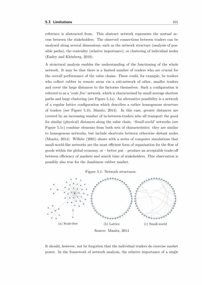
5.3 Limitations 101
reference is abstracted from. This abstract network represents the mutual ac-
cess between the stakeholders. The observed connections between traders can be
analysed along several dimensions, such as the network structure (analysis of pos-
sible paths), the centrality (relative importance), or clustering of individual nodes
(Easley and Kleinberg, 2010).
A structural analysis enables the understanding of the functioning of the whole
network. It may be that there is a limited number of traders who are crucial for
the overall performance of the value chains. These could, for example, be traders
who collect rubber in remote areas via a sub-network of other, smaller traders
and cover the large distances to the factories themselves. Such a configuration is
referred to as a ‘scale free’ network, which is characterised by small average shortest
paths and large clustering (see Figure 5.1a). An alternative possibility is a network
of a regular lattice configuration which describes a rather homogenous structure
of traders (see Figure 5.1b, Manitz, 2014). In this case, greater distances are
covered by an increasing number of in-between-traders who all transport the good
for similar (physical) distances along the value chain. ‘Small-world ’ networks (see
Figure 5.1c) combine elements from both sets of characteristics: they are similar
to homogenous networks, but include shortcuts between otherwise distant nodes
(Manitz, 2014). Wilhite (2001) shows with a series of computer simulations that
small-world-like networks are the most efficient form of organisation for the flow of
goods within the global economy, or – better put – produce an acceptable trade-off
between efficiency of markets and search time of stakeholders. This observation is
possibly also true for the Jambinese rubber market.
Figure 5.1: Network structures.
(a) Scale-free (b) Lattice (c) Small-world
Source: Manitz, 2014
It should, however, not be forgotten that the individual traders do exercise market
power. In the framework of network analysis, the relative importance of a single

102 Discussion of Results and Open Questions
trader in the network can be understood as an indicator of his or her bargaining
power (additional to other techniques such as the ones presented in this disserta-
tion). It can be assessed by a descriptive analysis of the fundamental structure of
the network, i. e. the position of individual nodes (traders) and their links. The
centrality, for example, captures the relative importance of nodes and comprises
the ’degree of centrality ’ (representing the number of connections from different
nodes) or - more sophisticated - the ’betweenness’ and ’closeness’: the betweenness
of one node indicates between how many nodes (on one path) it is positioned, and
the closeness the average distance to all other nodes in the network (Easley and
Kleinberg, 2010; Manitz, 2014). Most power arises from network-nodes that lie a)
on many paths along which the good can be traded and b) between many nodes
on each path (Easley and Kleinberg, 2010). In this application, the goal would be
to identify these most important traders, and see in what relation the margin they
receive stands to their function.
An analysis of the clustering within the network could provide insights on the
occurrence of groups of traders working together, which would indicate cooperation,
possibly collusion of the stakeholders that form these clusters. It is implemented
in the form of community detection algorithms that search for groups of nodes
that are disproportional highly interconnected, located in networks that exhibit an
otherwise relatively low number of links between the groups.
Paper two
The most important limitation of the paper presented in chapter three is that
it does not generate insights about the dynamics between the Jambinese rubber
processors. This is due to the fact that the analysis is carried out on an aggregate
level: the buying prices of the five factories enter as an average. Selling prices are
not differentiated between the factories either.
It is therefore not possible to draw conclusions regarding the relationship between
the five rubber processing factories. Their interactions could be of the nature of an
oligopsony or of monopsonistic competition. If it is an oligopsony, the individual
agents (factories) can either behave in a cooperative way (cartel case) or exhibit
non-cooperative behaviour. Each of the three cases would lead to a different equi-
librium, depending on the strategy each agent chooses to follow.
However, the observed equilibrium does not unambiguously indicate one under-
lying structure of the market. Under the assumption of a punishment model for
example, in which agents can pose a credible threat, even the non-cooperative be-
haviour within an oligopsony would lead to the cartel result. On the other hand,

5.3 Limitations 103
a cooperative behaviour does not necessarily result in the cartel solution (Perloff
et al., 2007).
In the case of the Jambinese rubber processors, a Bertrand framework concerning
the rubber input can be assumed: the processors set the prices for slabs of raw
rubber and the suppliers react by deciding upon the quantities that they sell to
each factory. If prices differ, the factory offering the highest price would be able
to purchase virtually all rubber that is offered at a particular point in time. A
cooperative behaviour is associated with a multilateral reduction of the price for the
raw rubber input, while non-cooperative behaviour is indicated by one stakeholders’
raise of his/her input price.
The focus of this work would be on strategic decisions and not so much on the
fundamentals (as laid out in the introduction to this work), since the fundamentals
are difficult to observe in contrast to input prices, which do not affect fundamentals.
Since the decisions in this competition concern prices, it is appropriate to allow for
continuous strategies, which means that the agents do not only have the choice on
whether to cooperate or not, but also on the extent of the (non-)cooperation, as
the decision variable – the input price – is continuous.
The target of the econometric analysis would be to determine the structure and the
strategies that produced the actual economic outcome. One approach is suggested
by Perloff et al. (2007) who present a method to estimate strategies directly. They
first theoretically reconstruct the different kinds of games that are played by two
stakeholders based on different assumptions on the nature of their relation. These
are solved to find the respective equilibria. Based on these theoretical findings
as well as empirical data, a model is estimated that enables the generation of
conclusions on which strategies are followed by the firms. The advantage of this
approach is that it enables the researcher ’to estimate firms’ strategies subject to
restrictions implied by game theory and test hypotheses based on these estimated
strategies’ (Perloff et al., 2007, p. 213). The data required for the Bertrand game
are time series data of input and output prices.
In their approach, Perloff et al. (2007) assume a sequence of static games, which
means that the agents only maximise current profits. This is in contrast to a
dynamic setting where agents also maximise future profits. The validity of this
assumption will need to be checked carefully. Another open question towards the
approach of Perloff et al. (2007), who consider two-player scenarios only, is whether
both theory and empirical estimation can be extended to an application with five
agents, as is the case in Jambi.
Alternatively it would also be possible to search for systematic differences and pat-
104 Discussion of Results and Open Questions
terns in the different agents’ reactions to international price changes with price
transmission analysis. These approaches include the analysis of spatial price trans-
mission between the five factories by estimating a spatial vector error correction
model, or to estimate a vertical price transmission model, consisting of the long run
equilibrium between each of the five factories’ prices and the world market price,
and then the vector error correction model.
Paper three
One possibly problematic assumption of this paper is that the EU is taken to
be one country. It is implicitly assumed to be a single point in which no trade
occurs. However, changing that would be a difficult thing to achieve, due to data
limitations. It is not very clear which EU member exactly imports the sugar
stemming from third countries. For the sake of the analysis which focuses on
the effects on third countries, this problem should be of limited relevance, however.
In the assessment part of the paper, the concept of welfare applied is not very
differentiated. It considers neither questions of inter- nor of intra-generational
justice, due to long-term externalities of agricultural production (see below).
This analysis is based on secondary data and therefore subject to the limitations
associated commonly with this kind of data. However, the most central variables –
trade flows and preferences (quotas) – were provided by Eurostat and the EU com-
mission which are assumed to be very reliable since the Eurostat data concerning
imports are generated from the European customs authorities. Other explanatory
variables such as the exchange rate and total sugar production are drawn from
official agencies, which in turn have to rely on data provided by the individual
countries, and are not necessarily accurate. The variables capturing the geograph-
ical distance between countries and the political system of the trade partners stem
from research institutes.
5.4 Relevance and wider implications
Greater welfare implications of rubber production
In chapters two and three, only malfunctioning on the demand side of this mar-
ket was scrutinised. When considering the supply side, the main failure might be
constituted by negative externalities stemming from the monoculture production
mode of rubber cultivation. These negative externalities have not been considered
in this work, but are of crucial importance when assessing the overall welfare effects
of rubber cultivation in Jambi. Some of them take effect on a local scale, such as

5.4 Relevance and wider implications 105
loss of biodiversity and reduced functionality of ecoservices (Barnes et al., 2014;
Rubiana et al., 2015), while others take effect on the global scale. Most notably,
global scale effects include the decomposition of existing carbon pools due to expo-
sure to aerobic conditions (Biagioni et al., 2015) as well as to erosion (Guillaume,
2015), reduced net primary production in above- and belowground tree biomass,
as well as a reduction in the long time accumulation of carbon (Kotowska et al.,
2015). The lowland peatlands of Southeast Asia are the largest in the tropics, and
are currently under threat. Indonesia’s handling of this situation has the potential
to produce serious effects, and is also likely to send a signal to other countries in a
similar position.
Since the costs are public, it is unlikely that the emissions which cause these costs
are taken into account via the market mechanisms. Therefore, private and social
costs fall apart, requiring an intervention from the government (Koester, 2011).
The appropriate response to this market failure would be taxes on the externalities
in order to reduce output to a welfare increasing level.
Two questions that emerge immediately at this point concern the valuation of
a ‘healthy environment’: what is the individual’s willingness to pay, and whose
willingness to pay is considered? The first question refers to the problem that it is
questionable whether the willingness to pay is actually an appropriate criterion for
the valuation of nature. Due to the long-term nature of effects that are experienced
far in the future, the current participants of the market may either not consider
them in their decisions, or have time preferences that favour the present (Coursey
et al., 1987). The view on a larger scale leads to the second question that considers
the temporal and geographical dimension of the individuals whose interests are
taken into account. Members of future generations, for example, have interests
that might be negatively affected by current decisions. Due to the global scale
of environmental and climatic processes, decision making practices on this issue
would also require the involvement of the global society.
Compared to other systems of political interventions (such as the one presented
in chapter four), the question here can be answered easier: the maximum levels
of pollution and usage of natural resources that enable future generations to offer
every individual the opportunity to enjoy the same quality of life that the cur-
rent generation has, are in fact known. Izrael and Semenov (2006) explain what
is required to reach the two degree target which is, in turn, necessary to avoid ir-
reversible changes of the climate, enabling future generations to live under similar
(climatic) conditions under which the current one does.
In a globalised world of international competition in the majority of goods, the
106 Discussion of Results and Open Questions
unilateral introduction of climate protecting regulations causes a competitive dis-
advantage. Therefore, as long as low environmental standards constitute a com-
parative advantage, countries are encouraged to engage in a race to the bottom
for the lowest standards. In order to avoid this competition, the externalities that
create effects on a global scale have to be regulated on an international level.
Other instances of market malfunctioning
In order to draw conclusions from past experiences such as the ones analysed in
this thesis, it is important to identify markets to which the concepts developed in
the individual papers of this thesis apply. The topics of market malfunctions that
were touched upon in this dissertation are also relevant in other instances. For
example, the analysis of possibly asymmetric transmission of prices can be used as
an indicator of market power in other cases. Examples of cartels can be found on
various levels. In the German food industry, from 2013 to 2014 alone, sanctions
were imposed in the beer industry (Bundeskartellamt, 2014b), on sausage makers
(Bundeskartellamt, 2014a), candy producers (Bundeskartellamt, 2013a), flour mills
(Bundeskartellamt, 2013b) and in the sugar industry (Bundeskartellamt, 2014b).
It would be interesting to see if any of these industries engaged in the asymmetric
transmission of prices. If firms have a strong market power both on the supply and
the demand side (for example the flour industry), challenges on a methodological
level are also present.
Other markets prone to preference erosion
Preference erosion as discussed in chapter four can be a serious concern whenever
external stakeholders enjoy preferential access to a protected market. There is a
lot of scope for preference erosion due to multilateral trade negotiations in which
countries participate that currently protect their markets via tariffs and also grant
preferences. However, Francois et al. (2006) find that even if all tariffs were
abolished, and preference erosion was expected to be maximal, the effects might
not be strongly felt because of an underuse of the preferences currently granted
for many products. The main reasons for this under-usage are the administrative
challenges facing the export countries, such as fulfilling the rules of origin.
Considering the trade between Indonesia and the European Union, the erosion
of other countries’ preferences is a more likely scenario. Success of the currently
ongoing negations concerning a free trade agreement between the EU and Indone-
sia (EU Commission: DG Trade, 2015) would cause preference erosion for ACP
countries that currently export palm oil to the EU under preferential treatment;
this is primarily because the EU prices have the potential to decrease. The EU,

5.4 Relevance and wider implications 107
however, argues that the ACP countries do not have much to lose. Since the most
favoured nation tariff is only 3.8%, the current preference margin enjoyed by the
ACP countries is relatively small (European Parliament, 2011, 2012).
Perhaps more relevant for Indonesia are the energy politics of the European Union,
more specifically the Renewables Directive, which formulates targets for the min-
imum share of energy from renewable sources for each member state (European
Parliament, 2009). In Germany, for example, this is realised via the Biofuel Quota
Act (Bundesgesetzblatt, 2006), amongst other measures. This law requires the
suppliers of car fuel to include a minimum amount of biofuel in the fuel they sell.
This increases the demand for energy-rich plants, such as the oil palm.
Based on the considerations from chapter four, one could argue that this leads
to the creation of production capacities in the palm oil sector that are only based
upon this European regulation. If the European policy changed, the demand would
decline and the production capacities would exceed this reduced demand.
However, since the central role of palm oil is one of an input in the production of
processed food, and the share of palm oil for energy production is rather small, the
overall impact of a changed energy policy would probably not cause too much harm.
Besides that, the EU constitutes only a relatively small market for Indonesian Palm
oil (in 2012, 14% of Indonesian palm oil exports went to the EU).5
Policy under constraints
The sugar case impressively shows the large number of policy constraints. For
sugar, these constraints are external (such as WTO membership) and internal (such
as limits with the European population’s acceptance of the size of the EU budget
and particularly its agricultural share). Under this consideration, it is intuitive
that any market based intervention has the potential to conflict with one or several
of these constraints, since these are exactly the two conditions that a policy has
to fulfil in order to be acceptable: social acceptance, especially the distributional
consequences, and compatibility with international agreements (Constanza et al.,
2001). Koester (2011) does not see these conditions as being fulfilled for many
parts of the Common Agricultural Policy, which conserves the status quo rather
than fostering innovation. The sugar policy in the timeframe under consideration is
representative of this. In the CMO for sugar, the external constraints are primarily
manifested by the introduction of a maximum amount of subsidised exports after
the Uruguay round of multilateral trade negotiations. This was followed by the
5Figures from Worldbank World Integrated Trade Solution. http://wits.worldbank.org, ac-cessed on 02.03.2015

108 Discussion of Results and Open Questions
lawsuit in which the WTO found the EU guilty of having trespassed this amount,
and eventually the necessary adjustment of the intervention price.
In general, these results call for policy makers to put effort into identifying all
stakeholders that are possibly affected by a planned intervention and do their best
in predicting the effects on each group before implementation. Furthermore, all
groups should be consulted before, and if possible included in the process of design-
ing the policy. This is especially relevant in the current context of the Indonesian
rubber market, when the failures described in chapters two and three are to be
addressed by policy in the near future.

Bibliography
Abbott, P. C. (2002). Tariff-rate quotas: failed market access instruments? Euro-
pean Review of Agriculture Economics, 29:109–130.
Adnan, N. A. and Atkinson, P. M. (2011). Exploring the impact of climate and
land use changes on streamflow trends in a monsoon catchment. International
Journal of Climatology, 31(6):815–831.
Agostino, M., Demaria, F., and Trivieri, F. (2010). Non-Reciprocal Trade Prefer-
ences and the Role of Compliance Costs in the Agricultural Sector: Exports to
the EU. Journal of Agricultural Economics, 61(3):652–679.
Aker, J. C. (2010). Information from markets near and far: Mobile phones and
agricultural markets in Niger. American Economic Journal: Applied Economics,
2:46–59.
Akiefnawati, R., Ayat, A., Alira, D., Suyitno, and Joshi, L. (2010). Enhancing
rubber production in communities around a village forest in Bungo District,
Jambi Province. In Leimona, B. and Joshi, L., editors, Eco-certified natural
rubber from sustainable rubber agroforestry in Sumatra, Indonesia., pages 25–31.
World Agroforestry Centre (ICRAF).
Anderson, J. E. (1979). A Theoretical Foundation for the Gravity Equation. Amer-
ican Economic Review, 69(1):106–116.
Anderson, J. E. and Van Wincoop, E. (2003). Gravity with Gravitas: A Solution
to the Border Puzzle. American Economic Review, 93(1):170–192.
Anderson, J. E. and Yotov, Y. V. (2010). The changing incidence of geography.
American Economic Review, 100(1):106–116.
Arifin, B. (2005). Supply-Chain of Natural Rubber in Indonesia. Jurnal Manajemen
Agribisnis, 2(1):1–16.
Bain, J. S. (1956). Barriers to new competition: their character and consequences
in manufacturing industries.
109
110 Bibliography
Baldwin, R. and Taglioni, D. (2007). Trade Effects of the Euro: a Comparison of
Estimators. Journal of Economic Integration, 22(4):780–818.
Barnes, A. D., Jochum, M., Mumme, S., Haneda, N. F., Farajallah, A., Widarto,
T. H., and Brose, U. (2014). Consequences of tropical land use for multitrophic
biodiversity and ecosystem functioning. Nature Communications, 5:5351.
Barnett, B. J., Barrett, C. B., and Skees, J. R. (2008). Poverty Traps and Index-
Based Risk Transfer Products. World Development, 36:1766–1785.
Bates, D. M. and Watts, D. G. (1988). Nonlinear Regression Analysis and Its
Applications. John Wiley & Sons, New York, USA.
Battese, G. E. (1997). A Note on the Estimation of Cobb-Douglas Production
Functions when some Explanatory Variables Have Zero Values. Journal of Agri-
cultural Economics, 48:250–252.
Bendix, D., Danielzik, C.-M., Doll, J., Holzwarth, S., Juergensohn, J., Kiesel, T.,
Kontzi, K., and Philipp, C. (2013). Mit Kolonialen Grußen. glokal e.V., Berlin,
2nd edition.
Bergstrand, J. H. (1985). The Gravity Equation in International Trade: Some
Microeconomic Foundations and Empirical Evidence. The Review of Economics
and Statistics, 67:474–481.
Berndt, E. R. (1996). The Practice of Econometrics: Classic and Contemporary.
Addison Wesley, Boston, har/dskt edition.
Bertrand (1883). Book Review on ”Theorie mathematique de la richesse sociale”
and ”Recherches sur les principes mathematiques de la richesse”. Journal des
Savants, pages 890–904.
Bhaskar, V., Manning, A., and To, T. (2002). Oligopsony and Monopsonistic
Competition in Labor Markets. Journal of Economic Perspectives, 16(2):155–
174.
Biagioni, S., Krashevska, V., Achnopha, Y., Saad, A., Sabiham, S., and Behling,
H. (2015). 8000 years of vegetation dynamics and environmental changes of
an unique inland peat ecosystem of the Jambi Province in Central Sumatra,
Indonesia. Under Review.
Bloom, D. E. and Canning, D. (2005). Health and Economic Growth: Reconciling
the Micro and Macro Evidence. Harvard School of Public Health, Cambridge,
MA: Working Paper.

Bibliography 111
Boisvert, R. N. (1982). The Translog Production Function - Properties, several In-
terpretations and Estimation Problems. Department of Agricultural Economics,
Cornell Univ: Working Paper.
Bosquet, C. and Boulhol, H. (2014). Applying the GLM Variance Assumption to
Overcome the Scale-Dependence of the Negative Binomial QGPML Estimator.
Econometric Reviews, 33(7):772–784.
Bresnahan, T. F. (1982). The oligopoly solution concept is identified. Economics
Letters, 10(1):87–92.
Bundesgesetzblatt (2006). Gesetz zur Einfuhrung einer Biokraftstoffquote durch
Anderung des Bundes-Immissionsschutzgesetzes und zur Anderung energie- und
stromsteuerrechtlicher Vorschriften (Biokraftstoffquotengesetz – BioKraftQuG).
Bundeskartellamt (2013a). Bußgeldverfahren gegen Hersteller von Sußwaren. Tech-
nical report, Bonn.
Bundeskartellamt (2013b). Bußgeldverfahren gegen Unternehmen der
Muhlenindustrie. Technical report, Bonn.
Bundeskartellamt (2014a). Bundeskartellamt imposes fines on sugar manufacturers.
Technical report, Bonn.
Bundeskartellamt (2014b). Bußgelder gegen Bierbrauer wegen verbotener Preisab-
sprachen. Technical report, Bonn.
Burbidge, J. B., Magee, L., and Robb, A. L. (1988). Alternative Transformations
to Handle Extreme Values of the Dependent Variable. Journal of the American
Statistical Association, 83:123–127.
Burnham, K. and Anderson, D. (2002). Model selection and multimodel inference:
a practical information-theoretic approach. Springer, Heidelberg, Germany.
Calı, M., Nolte, S., and Cantore, N. (2013). Sweet and sour changes in trade
regimes. The World Economy, 36(6):786–806.
Cardwell, M. (2004). The European Model of Agriculture. Oxford University Press
Oxford, New York.
Carrere, C., de Melo, J., and Tumurchudur, B. (2010). Disentangling market ac-
cess effects of preferential trading arrangements with an application for ASEAN
members under an ASEAN-EU FTA. The World Economy, 33:42–59.

112 Bibliography
Cassels, J. M. (1937). Monopolistic Competition and Economic Realism. Canadian
Journal of Economics, 3(3):376–393.
Chamberlin, E. H. (1958). The Theory of Monopolistic Competition – A Reorien-
tation of the Theory of Value. Harvard University Press, Cambridge, 7th edition.
Chaplin, H. and Matthews, A. (2006). Coping with the Fallout for Preference
Receiving Countries from EU Sugar Reform. The Estey Centre Journal of In-
ternational Law and Trade Policy, 7(1):15–31.
Chen, B. and Li, Y. (2014). Analyzing Bilateral Trade Barriers under Global Trade
Context: A Gravity Model Adjusted Trade Intensity Index Approach. Review
of Development Economics, 18(2):326–339.
Chetty, R., Guren, A., Manoli, D., and Weber, A. (2011). Are Micro and Macro
Labor Supply Elasticities Consistent? A Review of Evidence on the Intensive
and Extensive Margins. The American Economic Review, 101(3):471–475.
Chua, C. L., Kew, H., and Yong, J. (2005). Airline Code-Share Alliances and Costs:
Imposing Concavity on Translog Cost Function Estimation. Review of Industrial
Organization, 26:461–487.
Cipollina, M., De Benedictis, L., Vicarelli, C., and Salvatici, L. (2013). Dummies
for Policies or Policies for Dummies. A Montecarlo Gravity Experiment. Roma
Tre University, Dipartimento di Economia: Working Paper.
Cipollina, M., Laborde, D., and Salvatici, L. (2014). The Tide That Does Not
Raise All Boats. IFPRI Discussion Paper 01382.
Cipollina, M. and Salvatici, L. (2007). EU and developing countries: an analysis
of preferential margins on agricultural trade flows. TradeAg Project: Working
Paper 07/11.
Cipollina, M. and Salvatici, L. (2010). The trade impact of European Union agri-
cultural preferences. Journal of Economic Policy Reform, 13(1):87–106.
Conforti, P., Ford, D., Hallam, D., Rapsomanikis, G., and Salvatici, L. (2007).
The European Union preferential trade with developing countries. Total trade
restrictiveness and the case of sugar. Universita degli Studi del Molise, Economics
& Statistics: Working Paper.
Constanza, R., Cumberland, J., Daly, H., Goodland, R., and Norgaard, R. (2001).
Einfuhrung in die Okologische Okonomik. Lucius and Lucius, Stuttgart.

Bibliography 113
Conway, G. R. and Pretty, J. N. (1991). Unwelcome Harvest: Agriculture and
Pollution. Routledge, London, 5th edition.
Coursey, D., Hovis, J., and Schulze, W. (1987). The disparity between willingness
to accept and willingness to pay measures of value. The Quarterly Journal of
Economics, pages 679–690.
Dauvergne, P. (1993). The politics of deforestation in Indonesia. Pacific Affairs,
66(4):497–518.
Easley, D. and Kleinberg, J. (2010). Networks, crowds, and markets: Reasoning
about a highly connected world. Cambridge University Press, Cambridge.
Eilers, P. H. C. and Marx, B. D. (1996). Flexible smoothing with B-splines and
penalties. Statistical Science, 11(2):89–102.
Ellis, F. (2000). The Determinants of Rural Livelihood Diversification in Developing
Countries. Journal of Agricultural Economics, 51:289–302.
Engle, R. F. and Granger, C. W. J. (1987). Co-integration and Error Correction:
Representation, Estimation, and Testing. Econometrica, 55(2):251–276.
Escribano, A. (2004). Nonlinear Error Correction: the Case of Money Demand in
the United Kingdom (1878–2000). Macroeconomic Dynamics, 8:76–116.
EU Commission (2013). CAP Reform – an Explanation of the Main Elements.
Technical report, Brussels.
EU Commission: DG Trade (2015). Countries and regions: Indonesia. Technical
report, Brussels.
Euler, M., Krishna, V., Fathoni, Z., Hermanto, S., Schwarze, S., and Qaim, M.
(2012). Ecological and Socioeconomic Functions of Tropical Lowland Rain-
forest Transformation Systems (Sumatra, Indonesia), Household Survey 2012.
Gottingen, Germany; Jambi, Indonesia; Bogor, Indonesia; Georg-August Uni-
versity of Goettingen, Bogor Agricultural Uni.
European Parliament (2009). DIRECTIVE 2009/28/EC OF THE EUROPEAN
PARLIAMENT AND OF THE COUNCIL on the promotion of the use of en-
ergy from renewable sources and amending and subsequently repealing Directives
2001/77/EC and 2003/30/EC. Official Journal of the European Union, 140(16).
European Parliament (2011). Parliamentary questions - Preference erosion in ACP
countries. Technical report, Brussels.

114 Bibliography
European Parliament (2012). Parliamentary questions - Answer given by Mr De
Gucht on behalf of the Commission. Technical report, Brussels.
Fafchamps, M. and Gabre-Madhin, E. (2006). Agricultural markets in Benin and
Malawi. The African Journal of Agricultural and Resource Economics, 1:67–94.
Fafchamps, M. and Hill, R. V. (2008). Price Transmission and Trader Entry in
Domestic Commodity Markets. Economic Development and Cultural Change,
56(4):729–766.
Fafchamps, M. and Minten, B. (2002). Returns to social network capital among
traders. Oxford economic papers, 54:173–206.
Fathoni, Z. (2009). Evaluation of Market System and Market Integration for Rub-
ber Cultivation in Jambi Province - Indonesia. Masters Thesis, Bogor Agricul-
tural Institute, Bogor, Indonesia.
Faust, H., Schwarze, S., Beckert, B., Brummer, B., Dittrich, C., Euler, M., Gatto,
M., Hauser-Schaublin, B., Hein, J., Holtkamp, A. M., Ibanez, M., Klasen, S.,
Kopp, T., Krishna, V., Kunz, Y., Lay, J., Muß hoff, O., Qaim, M., Steinebach,
S., Vorlaufer, M., and M, W. (2013). Assessment of socio-economic functions of
tropical lowland transformation systems in Indonesia - Sampling Framework and
Methodological Approach. CRC990 Discusson Paper Series: Efforts Discussion
Paper 1.
Feenstra, R. C. (2002). Border Effects and the Gravity Equation: Consistent
Methods for Estimation. Scottish Journal of Political Economy, 49(5):491–506.
Feintrenie, L., Schwarze, S., and Levang, P. (2010). Are local people conservation-
ists? Analysis of transition dynamics from agroforests to monoculture planta-
tions in Indonesia. Ecology and Society, 15(4).
Fitzherbert, E. B., Struebig, M. J., Morel, A., Danielsen, F., Bruhl, C. A., Donald,
P. F., and Phalan, B. (2008). How will oil palm expansion affect biodiversity?
Trends in Ecology and Evolution, 23(10):538–545.
Francois, J., Hoekman, B., and Manchin, M. (2006). Preference erosion and mul-
tilateral trade liberalization. World Bank Economic Review, 20:197–216.
Fugazza, M. and McLaren, A. (2014). Market Access, Export Performance and
Survival: Evidence from Peruvian Firms. Review of International Economics,
22(3):599–624.
Bibliography 115
Gabszewicz, J. and Thisse, J.-F. (2000). Microeconomic theories of imperfect com-
petition. Cahiers d’economie politique, 37(1):47–99.
Gonzalo, J. (1994). Five alternative methods of estimating long-run equilibrium
relationships. Journal of Econometrics, 60(1):203–233.
Gotor, E. (2009). The Reform of the EU Sugar Trade Preferences toward Devel-
oping Countries in Light of the Economic Partnership Agreements. The Estey
Centre Journal of International Law and Trade Policy, 10(2):15–29.
Gourieroux, C., Monfort, A., and Trognon, A. (1984). Pseudo Maximum Likelihood
Methods: Theory. Econometrica, 52(3):681–700.
Groenewegen, P. (2009). English Marginalism: Jevons, Marshall, and Pigou. In
Samuels, W. J., Biddle, J. E., and Davis, J. B., editors, A Companion to The
Hisotry of Economic Thought, chapter 16, pages 249–261. Blackwell, Malden,
4th edition.
Guillaume, T. (2015). Losses of soil carbon by converting tropical forest to plan-
tations: Erosion and decomposition estimated by δ13C. Global Change Biology.
Hagedorn, K. (1983). Reflections on the methodology of agricultural policy re-
search. European Review of Agricultural Economics, 10(4):303–323.
Hallet, G. (1981). The Economics of Agricultural Policy. Basil Blackwell, Oxford,
2nd edition.
Hansen, B. E. and Seo, B. (2002). Testing for two-regime threshold cointegration
in vector error-correction models. Journal of Econometrics, Long Memory and
Nonlinear Time Series, 110(2):293–318.
Hassouneh, I., Radwan, A., Serra, T., and Gil, J. M. (2012). Food scare crises and
developing countries: The impact of avian influenza on vertical price transmission
in the Egyptian poultry sector. Food Policy, 37:264–274.
Hassouneh, I., Serra, T., and Gil, J. M. (2010). Price Transmission in the Spanish
Bovine Sector: The BSE Effect. Agricultural Economics, 41(1):33–42.
Head, K., Mayer, T., and Ries, J. (2009). How remote is the offshoring threat?
European Economic Review, 53(4):429–444.
Henningsen, A. and Henning, C. H. C. A. (2009). Imposing regional monotonicity
on translog stochastic production frontiers with a simple three-step procedure.
Journal of Productivity Analysis, 32:217–229.

116 Bibliography
Hirschman, A. (1964). The paternity of an index. The American Economic Review,
54:761–762.
Hoekman, B. and Howse, R. (2008). EC–Sugar. World Trade Review, 7(1):149–178.
Hornok, C. (2011). Gravity or Dummies? The Limits of Identification in Gravity
Estimations. CeFig: Working Paper 11/09.
Ihle, R., Brummer, B., and Thompson, S. R. (2012). Structural change in Euro-
pean calf markets: Decoupling and the blue tongue disease. European Review of
Agricultural Economics, 39:157–179.
Ivanov, V. and Kilian, L. (2005). A Practitioner’s Guide to Lag Order Selection
For VAR Impulse Response Analysis. Studies in Nonlinear Dynamics & Econo-
metrics, 9(1):1–36.
Izrael, Y. and Semenov, S. (2006). Critical levels of greenhouse gases, stabilization
scenarios, and implications for the global decisions. In Schellnhuber, H. J., edi-
tor, Avoiding dangerous climate change, pages 3–7. Cambridge University Press,
Cambridge.
Johansen, S. (1998). Likelihood-based inference in cointegrated vector autoregressive
models. Oxford University Press, Oxford.
Kinnucan, H. W. and Forker, O. D. (1987). Asymmetry in Farm-Retail Price Trans-
mission for Major Dairy Products. American Journal of Agricultural Economics,
69(2):285–292.
Koester, U. (2011). Grundzuge der landwirtschaftlichen Marktlehre. Franz Vahlen,
Munich.
Kojima, K. and Ozawa, T. (1984). Micro-and Macro-Economic Models of Direct
Foreign. Hitotsubashi Journal of Economics, 25(1):1–20.
Kopp, T., Alamsyah, Z., Fatricia, R. S., and Brummer, B. (2014). Have Indonesian
Rubber Processors Formed a Cartel? Analysis of Intertemporal Marketing Mar-
gin Manipulation. CRC990 Discussion Paper Series: Efforts Discussion Paper
3.
Kopp, T. and Brummer, B. (2015). Moving Rubber to a Better Place – and
Extracting Rents from Credit Constrained Farmers along the Way. CRC990
Discussion Paper Series: Efforts Discussion Paper 9.
Bibliography 117
Kotowska, M., Leuschner, C., Antono, T., Meriem, S., and Hertel, D. (2015).
Quantifying above- and belowground biomass carbon loss with forest conversion
in tropical lowlands of Sumatra (Indonesia). Under Review.
Krivobokova, T., Kneib, T., and Claeskens, G. (2010). Simultaneous Confidence
Bands for Penalized Spline Estimators. Journal of the American Statistical As-
sociation, 105(490):852–863.
Krueger, A. O. (1974). The Political Economy of the Rent-Seeking Society. The
American Economic Review, 64:291–303.
Lloyd, T. A., McCorriston, S., Morgan, C. W., and Rayner, A. J. (2006). Food
Scares, Market Power and Price Transmission: The UK BSE Crisis. European
Review of Agricultural Economics, 33(2):119–147.
Mairesse, J. and Jaumandreu, J. (2005). Panel-data estimates of the production
function and the revenue function: What difference does it make? Scandinavian
Journal of Economics, 107:651–672.
Manitz, J. (2014). Statistical Inference for Propagation Processes on Complex
Networks. Dissertation.
Marcuzzo, M. (2009). The “First” Imperfect Competition Revolution. In Samuels,
W. J., Biddle, J. E., and Davis, J. B., editors, A companion to the history of
economic thought, chapter 19. Blackwell, Malden, 4th edition.
Martini, E., Akiefnawati, R., Joshi, L., Dewi, S., Ekadinata, A., Feintrenie, L.,
and van Noordwijk, M. (2010). Rubber agroforests and governance at the in-
terface between conservation and livelihoods in Bungo district, Jambi province,
Indonesia. World Agroforestry Centre: Working Paper.
McCorriston, S., Morgan, C. W., and Rayner, A. J. (2001). Price transmission:
the interaction between market power and returns to scale. European Review of
Agricultural Economics, 28(2):143–159.
McMillan, M., Rodrik, D., and Welch, K. H. (2002). When Economic Reform
Goes Wrong: Cashews in Mozambique. National Bureau of Economic Research:
NBER Working Paper.
Medema, S. (2009). The economic role of government in the history of economic
thought. In Samuels, W. J., Biddle, Jeff, E., and Davis, J. B., editors, A com-
panion to the history of economic thought, chapter 27. Blackwell, Malden, 4th
edition.

118 Bibliography
Meyer, J. and von Cramon-Taubadel, S. (2004). Asymmetric Price Transmission:
A Survey. Journal of Agricultural Economics, 55(3):581–611.
Morey, E. R. (1986). An Introduction to Checking , Testing , and Imposing Curva-
ture Properties : The True Function and the Estimated Function. The Canadian
Journal of Economics, 19(2):207–235.
Nedergaard, P. (2006). Market failures and government failures: A theoretical
model of the common agricultural policy. Public Choice, 127:393–413.
Nicita, A. (2011). Measuring the relative strength of preferential market access.
United Nations UNCTAD Policy Issues in International Trade and Commodities
Study Series No 47.
Nicita, A. and Rollo, V. (2013). Tariff Preferences As A Determinant For Exports
From Sub-Saharan Africa. United Nations UNCTAD Policy Issues in Interna-
tional Trade and Commodities Study Series No. 60.
Nolte, S., Buysse, J., and Van Huylenbroeck, G. (2012). Modelling the effects of
an abolition of the EU sugar quota on internal prices, production and imports.
In European Review of Agricultural Economics, volume 39, pages 75–94.
Osborne, T. (2005). Imperfect competition in agricultural markets: Evidence from
Ethiopia. Journal of Development Economics, 76:405–428.
Peramune, M. R. and Budiman, A. (2007). A Value Chain Assessment of the Rub-
ber Industry in Indonesia. U.S. Agency for International Development. Project
Report, USAid.
Perloff, J. M., Karp, L. S., and Golan, A. (2007). Estimating Market Power and
Strategies. Cambridge University Press, New York, USA.
Pigou, A. (1932). The Economics of Welfare. Macmillan, London, 4th edition.
Pitt, M. (1980). Alternative Trade Strategies and Employment in Indonesia. In
Krueger, A. O., Lary, H. B., Monson, T., and Akrasanee, N., editors, Trade
and Employment in Developing Countries, 1: Individual Studies. University of
Chicago Press, Chicago.
Piyapromdee, S., Hillberry, R., and MacLaren, D. (2014). ’Fair trade’ coffee and
the mitigation of local oligopsony power. European Review of Agricultural Eco-
nomics, 41(4):537–559.

Bibliography 119
Pokhrel, D. M. and Thapa, G. B. (2007). Are marketing intermediaries exploiting
mountain farmers in Nepal? A study based on market price, marketing margin
and income distribution analyses. Agricultural Systems, 94:151–164.
Prehn, S., Brummer, B., and Glauben, T. (2012). Structural gravity estimation
& agriculture. Department for Agricultural Economics and Rural Development:
Working Paper.
Raimondi, V., Scoppola, M., and Olper, A. (2012). Preference erosion and the de-
veloping countries exports to the EU: a dynamic panel gravity approach. Review
of World Economics, 148(4):707–732.
Regional Account and Statistical Analysis Division (2012). Jambi in Figures 2011.
BPS Statistics of Jambi Province, Jambi, Indonesia.
Robilliard, A.-S. and Robinson, S. (2003). Reconciling household surveys and
national accounts data using a cross entropy estimation method. Review of
Income and Wealth, 49:395–406.
Robinson, J. (1959). The Economics of Imperfect Competition. Macmillan & Com-
pany Limited, New York, 2nd edition.
Robinson, S. (1991). Macroeconomics, financial variables, and computable general
equilibrium models. World Development, 19(11):1509–1525.
Rubiana, R., Rizali, A., Denmead, L. H., Alamsari, W., Hidayat, P. P., Hindayana,
D., Clough, Y., Tscharntke, T., and Buchori, D. (2015). Agricultural Land Use
Alters Species Composition but not Species Richness of Ant Communities. Under
Review.
Runge, C. and Myers, R. (1985). Shifting foundations of agricultural policy analy-
sis: welfare economics when risk markets are incomplete. Journal of Agricultural
Economics, 67(5):1010–1016.
Ryan, D. L. and Wales, T. J. (2000). Imposing local concavity in the translog and
generalized Leontief cost functions. Economics Letters, 67:253–260.
Santos Silva, J. M. C. and Tenreyro, S. (2006). The log of gravity. The Review of
Economics and Statistics, 88(4):641–658.
Schmalensee, R. (1989). Inter-Industry Studies of Structure and Performance. In
Handbook of Industrial Organization, volume 2, pages 952–1009.

120 Bibliography
Serra, T., Gil, J. M., and Goodwin, B. K. (2006). Local Polynomial Fitting and
Spatial Price Relationships: Price Transmission in EU Pork Markets. European
Review of Agricultural Economics, 33(3):415–436.
Sraffa, P. (1926). The Laws of Returns under Competitive Conditions. The Eco-
nomic Journal, 36:535–550.
Statistics of Jambi Province (2013). Jambi in Figures 2012. Regional Account and
Statistical Analysis Division, Jambi.
Subramanian, A. and Qaim, M. (2011). Interlocked village markets and trader
idiosyncrasy in rural India. Journal of Agricultural Economics, 62:690–709.
Sujarwo, R. M., Kopp, T., Nurmalina, R., Asmarantak, R. W., and Brummer, B.
(2014). Choice of Marketing Channels by Rubber Small Traders in the Jambi
Province, Indonesia. Tropentag 2014: Conference Proceedings.
Tangermann, S. (1997). A Developed Country Perspective of the Agenda for the
Next WTO Round of Agricultural Negotiations. Occasional Paper, page WTO
Series Number 5.
Tinbergen, J. (1962). Shaping the World Economy; Suggestions for an Interna-
tional Economic Policy. Twentieth Century Fund, New York.
Varian, H. (1987). Intermediate microeconomics: a modern approach. Norton &
Company, New York, 1st edition.
von Cramon-Taubadel, S. (1998). Estimating asymmetric price transmission with
the error correction representation: An application to the German pork market.
European Review of Agricultural Economics, 25:1–18.
Vuong, Q. H. (1989). Likelihood ratio tests for model selection and non-nested
hypotheses. Econometrica: Journal of the Econometric Society, 57:307–333.
Westerlund, J. and Wilhelmsson, F. (2011). Estimating the gravity model without
gravity using panel data. Applied Economics, 43(6):641–649.
Wilhite, A. (2001). Bilateral trade and ’small-world’networks. Computational Eco-
nomics, 18(1):49–64.
Wood, S. N. (2003). Thin plate regression splines. Journal of the Royal Statistical
Society. Series B (Statistical Methodology), 65(1):95–114.
World Bank (2007). World Development Report 2008: Agriculture for Development.
Oxford University Press, New York.

Bibliography 121
Zellner, A., Kmenta, J., and Dreze, J. (1966). Specification and Estimation of
Cobb-Douglas Production Function Models. Econometrica, 34:784–795.

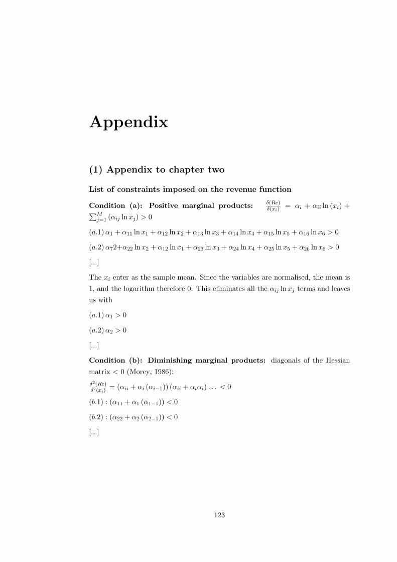
Appendix
(1) Appendix to chapter two
List of constraints imposed on the revenue function
Condition (a): Positive marginal products: δ(Re)δ(xi)
= αi + αii ln (xi) +∑Mj=1 (αij lnxj) > 0
(a.1)α1 + α11 lnx1 + α12 lnx2 + α13 lnx3 + α14 lnx4 + α15 lnx5 + α16 lnx6 > 0
(a.2)α72+α22 lnx2 + α12 lnx1 + α23 lnx3 + α24 lnx4 + α25 lnx5 + α26 lnx6 > 0
[...]
The xi enter as the sample mean. Since the variables are normalised, the mean is
1, and the logarithm therefore 0. This eliminates all the αij lnxj terms and leaves
us with
(a.1)α1 > 0
(a.2)α2 > 0
[...]
Condition (b): Diminishing marginal products: diagonals of the Hessian
matrix < 0 (Morey, 1986):
δ2(Re)δ2(xi)
= (αii + αi (αi−1)) (αii + αiαi) . . . < 0
(b.1) : (α11 + α1 (α1−1)) < 0
(b.2) : (α22 + α2 (α2−1)) < 0
[...]
123

124 Appendix
Detailed results of production function estimation
Elasticities at sample mean Unconstrained Constrained
ln x1 Rubber 1.0268*** 1.0236(0.0732)
ln x2 RespWork 0.0485*** 0.0156(0.0001)
ln x3 TranspCapacity -0.0214 0.0137(0.274)
ln x4 Distance 0.0105 0.0118(0.4426)
ln x7 Credit 0.0019* 0.0003(0.0735)
ln x1 square -0.014 -0.0056(0.3829)
ln x2 square 0.013 -0.0006(0.3673)
ln x3 square 0.0206* -0.0048(0.0.0909)
ln x4 square -0.0108 -0.0027(0.1225)
ln x7 square 0.0001* -0.0001(0.0698)
ln x1 ln x2 0.0082 -0.0001(0.3939)
ln x1 ln x3 0.0064 0.0005(0.5154)
ln x1 ln x4 0.0011 0.0019(0.9021)
ln x1 ln x7 0.0001 0.0001(0.5940)
ln x2 ln x3 -0.0372*** -0.0015(0.0002)
ln x2 ln x4 -0.0123* -0.0002(0.0002)
ln x2 ln x7 0.0001*** 0.0001(0.0001)

5.4 (1) Appendix to chapter two 125
ln x3 ln x4 0.0028 0.0011(0.7225
ln x3 ln x7 0.0001 0.0001(0.0509)
ln x4 ln x7 0.0001 -0.0027(0.3293)
dummy x2 -00732. -0.502***(0.3613) (0.0001)
dummy x3 -0.0035 0.0252(0.8839) (0.4793)
dummy x4 -0.087* 0.0928(0.0565) (0.1154)
dummy x7 1.276* -0.3314***(0.0728) (0.0001)
Constant -1.274*** 0.0764(0.0732)
Observations 209 209R-squared 0.987 0. 986
P values in parentheses*** p<0.01, ** p<0.05, * p<0.1

126 Appendix
(2) Appendix to chapter three
Error correction process (simple / symmetric adjustment)
Johansen Johansen Engle-GrangerTwo-Step
D ln pSell D ln pBuy D ln pBuy
L.ect -0.0153 -0.0593*** -0.0583***(0.511) (8.47e-08) (2.62e-05)
LD.ln pBuy -0.119 0.0548 0.0544(0.120) (0.134) (0.280)
L2D.ln pBuy 0.0987 -0.0192 -0.0192(0.190) (0.594) (0.711)
L3D.ln pBuy -0.0879 0.0365 0.0365(0.223) (0.289) (0.372)
L4D.ln pBuy 0.000486 0.130*** 0.130**(0.994) (5.45e-05) (0.0400)
LD.ln pSell 0.112** 0.155*** 0.157***(0.0151) (0) (2.00e-08)
L2D.ln pSell -0.0818* 0.138*** 0.139***(0.0776) (3.69e-10) (6.77e-06)
L3D.ln pSell 0.0467 0.109*** 0.109***(0.311) (7.39e-07) (5.06e-05)
L4D.ln pSell -0.0294 0.0360* 0.0364(0.507) (0.0883) (0.256)
Constant 0.000806 -0.000207 0.000500(0.340) (0.606) (0.247)
Observations 701 701 701
P values in parentheses*** p<0.01, ** p<0.05, * p<0.1
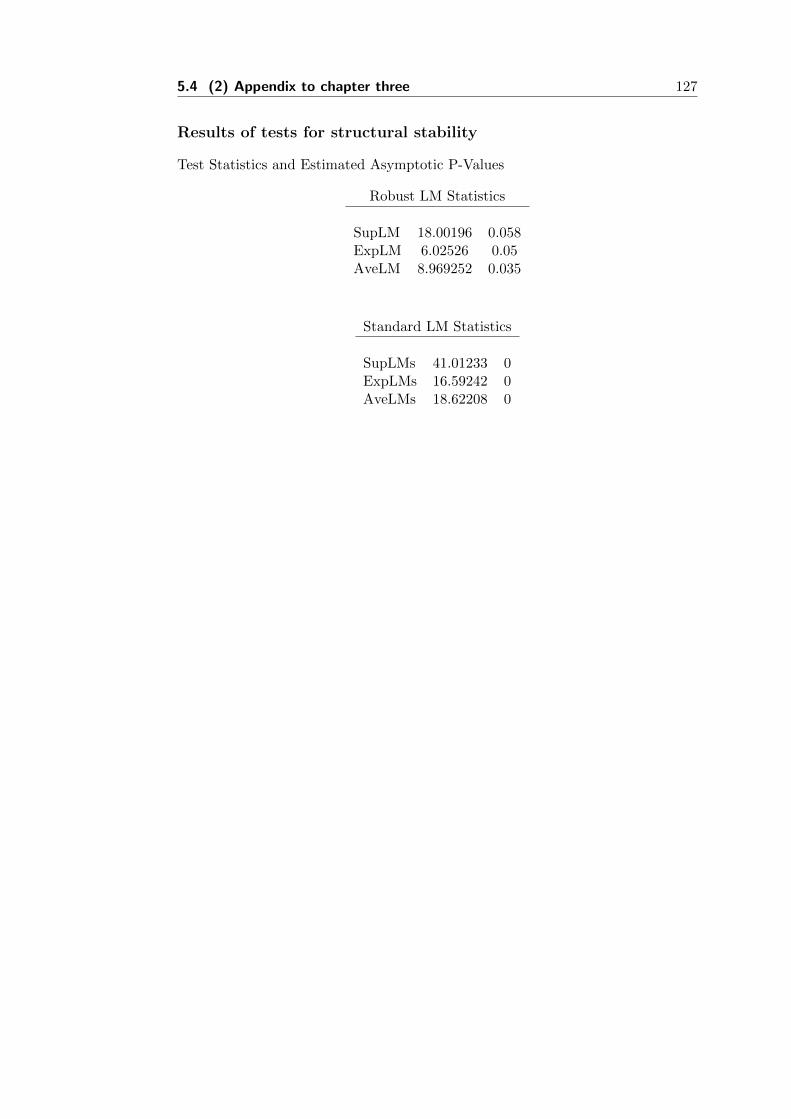
5.4 (2) Appendix to chapter three 127
Results of tests for structural stability
Test Statistics and Estimated Asymptotic P-Values
Robust LM Statistics
SupLM 18.00196 0.058ExpLM 6.02526 0.05AveLM 8.969252 0.035
Standard LM Statistics
SupLMs 41.01233 0ExpLMs 16.59242 0AveLMs 18.62208 0

128 Appendix
(3) Questionnaire
This is the questionnaire that was used for the data collection in Jambi, Indonesia.
The survey was conducted with the Bahasa Indonesia version of this question-
naire.

CRC – 990 – C01 – WP2 Kuesioner Lapangan Jambi 2012
Universitas Georg-August, Goettingen, 37073 Göttingen, Jerman
1
Trader Field Questionnaire
Introduction: Good morning. Our names are ________________ and ___________. We are doing a study on the role of traders in marketing of rubber and palm oil in Jambi province. The target of this study is to find out how the markets function on the local scale and to identify the deficiencies that constrain the business of all stakeholders involved. This will help us to increase the opportunities of everybody! I would like to ask for your permission to participate in our questionnaire which will take around 120-150 minutes. For taking your time we will give you this very nice T-Shirt when our questions are answered. You will also get this pen in the end. All the information you provide will be treated confidentially. That means that the data will be anonymised: your personal information will be detached from your other answers, so nobody will know which are the answers you gave. If you are interested, we will provide you with a copy of the results of our study (ready in around two years). We use your phone number only if we have further questions and won’t give it to anybody else. Do you want to participate in the survey? YA TIDAK Are you interested in receiving the results? YA TIDAK Instructions for Enumerator: Please tick the according answer like this: In case you ticked a wrong box please fill it completely like this: and tick the correct box like this: In case you filled a box completely but you want to tick it, please set a cross next to it, like this: If a trader is active in Palm Oil AND Rubber: Reply all questions that are marked “” only concerning Rubber!
1. Trader Identification and Enumerator Details 1.1. Respondent ID (from List):
……………………………..………
1.2. Name of respondent:
…………………
1.3. Name of village and district
……………………..
1.4. Name of enumerator who filled out this
questionnaire:
………………….
1.5. Name of other enumerator
………………….
1.6. Enumerator-Team:
A
1.7. Date of the interview: ………………….
1.8. Starting Time of Interview: ……………..
1.9. Gender of respondent:
MALE FEMALE
1.10. Status of respondent:
(all suppliers only
from same village)
(suppliers from this Kecamatan)
(suppliers from the whole Kabupaten)
Employee

CRC – 990 – C01 – WP2 Kuesioner Lapangan Jambi 2012
Universitas Georg-August, Goettingen, 37073 Göttingen, Jerman
2
1.11. If Employed: by what kind of business?
Pedagang Desa Pedagang Kecamatan Pedagang Kabupaten If Employed: answer all the future questions for your employer unless stated otherwise. 1.12. What is the name under which the
business operates? (if Trader, write
Pedagang)
………………………………….
1.13. Contact Information:
Phone number………………………
Email Address: ………………………
1.14. Does the respondent represent
somebody else?
YA TIDAK
1.15. Jika 1.14=YA: Who is represented?
……………………………………………
1.16. Jika 1.14=YA: Why is the originally
selected trader not answering?
Shop found, but trader could not be
found
Shop found, but respondent refused
Shop found, but appears to be out of
business
Shop not found
Others (specify)
………………………..
2. Characteristics of the Business 2.1. Ownership
2.1.1. How many shareholders are in the business? …………………………….
2.1.2. If there are more than one owner:
Which share do you own?
…………..%
2.1.3. If there are more than one owner: How
much do the other ones own (how
many percent each)?
1: …..% (Respondent)
2: …..%
3: ..…%
4: ...…%
5: ...…%
6: ...…%
7: …..%
2.1.4. Do you have a specific function in the
village?
YES TIDAK
2.1.5. Jika 2.1.4=YA: Which function?
………………………………..
2.1.6. What are your sources of income? trading : karet kelapa sawit
: masukan (Seperti: pupuk, atau benih, pestisida, etc.)
production : karet kelapa sawit labour salary in this business:
……………………..
Warung Toko Lease out land (how many ha? ….) other1: …………………………………….. other2: …………………………………….. other3: ……………………………………..
2.1.7. How much income do you generate
with each activity per bulan? Trading karet: Rp. .......... Trading kelapa Sawit Rp. ….. Trading inputs: …………………. Produksi Karet: Rp. ……….. Produksi Kelapa Sawit: Rp........... Salary: Rp........... Warung: Rp........... Toko: Rp. ……… Lease out land Rp. ….. Other1: Rp........... Other2: Rp........... Other3: Rp. ..........
2.1.8. How much time do you spend for
each activity per week? Trading: K …. hours/day | ……. days/week Trading: K.-S…. hours/day | ……. days/week Trading: input…. hours/day | ……. days/week Produksi K.: …. hours/day | ……. days/week Produksi K.-S:…. hours/day | ……. days/week Salary: .......... hari | ……… jam / week Warung: …. hours/day | ……. days/week Toko: …. hours/day | ……. days/week

CRC – 990 – C01 – WP2 Kuesioner Lapangan Jambi 2012
Universitas Georg-August, Goettingen, 37073 Göttingen, Jerman
3
Lease out land …. hours/day | ……. days/week Other1: …. hours/day | ……. days/week
Other2: …. hours/day | ……. days/week Other3: …. hours/day | ……. days/week
2.2. Overview Trading Activities
(Instruction for enumerator: many questions in this section can be understood as related to the produksi. always say that you are talking about the trading activities!) 2.2.1. What type of product do you trade
with?
2.2.2. What other products besides Rubber and Palm Oil do you market in your business? (not in warung) Lainnya 1: ………………………… Lainnya 2: …………………………
2.2.3. How many tons per month do you produce?
Karet ……ton Kelapa sawit …ton …………... (lainnya1): ……ton …………... (lainnya2): ……ton
2.2.4. How many tons per month do you buy from other producers / traders ?
Karet ……ton Kelapa sawit …ton …………... (lainnya1): ……ton …………... (lainnya2): ……ton
2.2.5. How long in total have you been a trader untuk karet?.……… years untuk kelapa sawit? ……….. years
2.2.6. Did you have any starting capital for your trading business?
2.2.7. What was the major source of start-up
capital for this business?
-family
members Loan from bank
BANSOS (Bantuan Social / Social
Help) (e.g. dari NGO) Help from the Government 2.2.8. If somebody wants to become a
trader, what is the minimum of capital this person must have? Rp. ……………
2.2.9. Where does your liquidity for buying rubber or palm oil come from?
2.2.10. Where does your liquidity for giving
credit to providers (farmers, other traders) come from?
fy) …………………….. 2.2.11. Do you keep written notes of the
following activities? Buying prices (Palm Oil/Rubber):
Selling prices (Palm Oil/Rubber): ry single transaction
Traded amounts (PalmOil/Rubber):
Credits given:
2.2.12. How many other traders are in the
dusun? Karet: ………………….. Sawit: …………………………
2.2.13. How many other traders are in the village? Karet: …….……………… Sawit: ……………………………
2.2.14. When was this village founded? ………
2.2.15. Is this a transmigrasi village?

CRC – 990 – C01 – WP2 Kuesioner Lapangan Jambi 2012
Universitas Georg-August, Goettingen, 37073 Göttingen, Jerman
4
2.3. Human Capital:
2.3.1. How many people work in the business (except of family members)? …………….. people
If more than five: fill out the following questions for the five most important ones
Person 1 activity: …………………….. Person 2 activity: …………………….. Person 3 activity: …………………….. Person 4 activity: …………………….. Person 5 activity: ……………………..
2.3.2. In which part of your business is each
of them employed? Person 1:
Production Trading Person 2:
Production Trading Person 3:
Production Trading Person 4:
Production Trading Person 5:
Production Trading 2.3.3. How many hours do they work?
Person 1 : …hours/week Person 2 : …hours/week Person 3 : …hours/week
Person 4 : …hours/week Person 5 : …hours/week
2.3.4. How are the workers paid?: Person 1: Salary: ….. per day:
Share of profit: ……. % Share of harvest: …… %
Person 2: Salary: ….. per day: Share of profit: ……. % Share of harvest: …… %
Person 3: Salary: ….. per day: Share of profit: ……. % Share of harvest: …… %
Person 4: Salary: ….. per day: Share of profit: ……. % Share of harvest: …… %
Person 5: Salary: ….. per day: Share of profit: ……. % Share of harvest: …… %
2.3.5. What did you spend on labour salary
in the last week? Person 1: ………….. Person 2: ………….. Person 3: ………….. Person 4: ………….. Person 5: …………..
2.4. Taking Credit
2.4.1. Which institutions are in your village where you can take a loan from? (multiple answers possible)
None Bank Microfinance scheme (Informal) money lender Warehouse Government program KUD
Else (specify) ……………………………
2.4.2. Specification of all the credits you took during the last 6 months
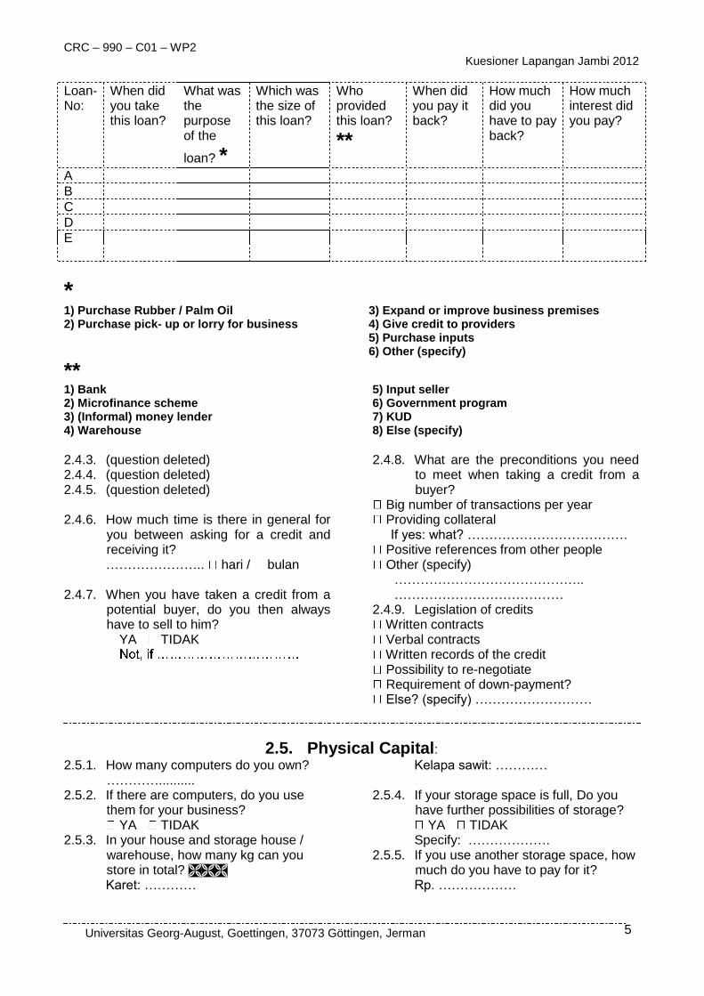
CRC – 990 – C01 – WP2 Kuesioner Lapangan Jambi 2012
Universitas Georg-August, Goettingen, 37073 Göttingen, Jerman
5
Loan- No:
When did you take this loan?
What was the purpose of the
loan? *
Which was the size of this loan?
Who provided this loan? **
When did you pay it back?
How much did you have to pay back?
How much interest did you pay?
A
B
C
D
E
* 1) Purchase Rubber / Palm Oil 3) Expand or improve business premises 2) Purchase pick- up or lorry for business 4) Give credit to providers
5) Purchase inputs 6) Other (specify)
**
1) Bank 2) Microfinance scheme 3) (Informal) money lender 4) Warehouse
5) Input seller 6) Government program 7) KUD 8) Else (specify)
2.4.3. (question deleted) 2.4.4. (question deleted) 2.4.5. (question deleted)
2.4.6. How much time is there in general for
you between asking for a credit and receiving it? ………………….. hari / bulan
2.4.7. When you have taken a credit from a potential buyer, do you then always have to sell to him?
YA TIDAK
2.4.8. What are the preconditions you need to meet when taking a credit from a buyer?
Big number of transactions per year Providing collateral
If yes: what? ………………………………. Positive references from other people Other (specify)
…………………………………….. ………………………………… 2.4.9. Legislation of credits
Written contracts Verbal contracts Written records of the credit Possibility to re-negotiate Requirement of down-payment? Else? (specify) ………………………
2.5. Physical Capital: 2.5.1. How many computers do you own?
………….......... 2.5.2. If there are computers, do you use
them for your business? YA TIDAK
2.5.3. In your house and storage house / warehouse, how many kg can you store in total? Karet: …………
Kelapa sawit: ………… 2.5.4. If your storage space is full, Do you
have further possibilities of storage? YA TIDAK
Specify: ………………. 2.5.5. If you use another storage space, how
much do you have to pay for it? Rp. ………………

CRC – 990 – C01 – WP2 Kuesioner Lapangan Jambi 2012
Universitas Georg-August, Goettingen, 37073 Göttingen, Jerman
6
2.5.6. Do you rent any vehicle on a regular basis? YA TIDAK 2.5.7. Do you own any motorized vehicle? YA TIDAK 2.5.8. Information on vehicles that you own: NO Type of
vehicle (name: Motorbike, car, truck, etc..) and brand.
Type of vehicle*
Capacity of this vehicle (tons) (if not for load: write “only people”)
When was it bought?
For how long more can you approximately use it?
What would be the price of selling this vehicle right now? (market value?)
Purpose: **
Do you rent it out? If yes: for
how many Rp/day?
1
2
3
4
5
6
7
8
9
*: 1) Motorcycle 2) Private Car 3) Pick Up 4) Truck
**: 1: picking up palm oil 2: picking up rubber 3: delivering palm oil 4: delivering rubber 5: picking up inputs 6: delivering inputs 7: others (specify): ………..
2.6. Land
2.6.1. How much land do you own?
………….. ha 2.6.2. Is it in one piece or fragmented?
one piece fragmented 2.6.3. If fragmented, how many pieces:

CRC – 990 – C01 – WP2 Kuesioner Lapangan Jambi 2012
Universitas Georg-August, Goettingen, 37073 Göttingen, Jerman
7
……………..……………..
2.6.4. Information on the fields
Field NO
Size (ha)
Do you have a land certificate for this? (Y / N / )
What is the land used for?
*
Is this land already producing?
Since when do you have it? (month / year)
How did you get it?
**
What would be the price of selling this field right now?
Who is working on the
land? ***
1
2
3
4
5
6
7
8
*:
1) Kelapa Sawit 2) Karet
3) Rice 4) Lainnya (specify)
**:
1) Bought 2) Inhereted
3) Transmigrasi 4) Else (specify)
***:
1) Family members 2) Labourers
3) Else (specify) 4) Respondent
2.6.5. Do you lease out any land?
YA TIDAK Since when? …….. months How much? ……………ha
2.6.6. Do you have any sharecropping arrangements in place?
YA TIDAK 2.6.7. Jika 2.6.6=YA: since when are are
they in place? Since ………. years
2.6.8. Jika 2.6.6=YA: How many ha and with how many people? ……….. ha ………… orang Is this included in the table above?
YA TIDAK
2.6.9. Jika 2.6.6=YA: Who takes the decision concerning:
What is cultivated? Respondent Petani
How to cultivate? Respondent Petani
When to sell? Respondent Petani
Whom to sell? Respondent Petani
2.6.10. Do you “offer” new sharecropping contracts?
YA TIDAK 2.6.11. Are you allowed to use land in
communal area (forest e.g.)? YA TIDAK
How much? ………….. ha

CRC – 990 – C01 – WP2 Kuesioner Lapangan Jambi 2012
Universitas Georg-August, Goettingen, 37073 Göttingen, Jerman
8
3. Business activities I
3.1. Palm Oil / Rubber Trade (towards downstream, i.e. buyers) 3.1.1. Rubber: What do you understand by KKK (“Kader Kering Karet”) and „Basi“?
KKK: ………………………………. Basi: ……………………………………
3.1.2. palm oil: What do you understand by “rendemin sawit”? rendomen……………………………….………………………………. ……………………………….……………………………….
3.1.3. Information on the firms that are your most important buyers of
Three most important buyers
1 2 3
a) Type of buyer *
b) Name of buyer (if factory / warehouse:name of factory / warehouse)
If gudang: is it acting as commission agent (facilitates, get’s share of traded value), or as a trader (buying & selling)?
What is the name of the person who you talk to?
What is the status of this person? - agen komisi - employee of the business named above - owner of the business named above - self-employed (toke) - self-employed (pedagang lebih besar)
What is the ethnic group of this person? 1: Jambi Kota 2a: Jambi Desa 2b: Jawa 3: Cina 4: Lainnya: …
Is this person employedor self-employed) ( E / S.-E.)
t) Are you registered in this institution as a trader (Y / T)
u) Is the institution that you deliver to also the institution where you get the money from? (Y / T)
c) When did the business relationship start?
d) When did it end? (leave blank if ongoing)
e) Where ist the firm located?
1. In the same village (Y / N)
2. Jambi City (Y/N)
3. Country (If not in Indonesia)
4. Province (If not in Jambi)
5. Regency (Kabupaten)
6. District (kecamatan)

CRC – 990 – C01 – WP2 Kuesioner Lapangan Jambi 2012
Universitas Georg-August, Goettingen, 37073 Göttingen, Jerman
9
7. Village
8. Dusun
h) Within how many days do you get paid? (Y=”immediately”)
i) Does the quality that you get paid vary every week? (Quality for rubber: basi content, KKK, etc., quality for oil palm: age of palm) (Y / T)
j) Does the quality that you get paid vary only between rainy and dry season? (Y / T)
k) Do you always get paid the same quality? (Y / T)
l) What price did you recive last week? (Rp./kg)
m) What price did you recive three months ago? (Rp./kg)
n) Is there a difference in price whether rubber has been stored in box or sack? (Ya / Tidak)
o) How many tons of Rubber/ Palm Oil did you sell to this firm in total in the last September?
K: …. ton K.-S.: ..… ton
K: …. ton K.-S.: ..… ton
K:…. ton K.-S.: ..… ton
How many rupiahs did you get paid for this amount?
K: Rp. …. K.-S.: Rp. ..…
K: Rp. …. K.-S.: Rp. ..…
K: Rp. …. K.-S.: Rp. ..…
p) How many separate deliveries of Palm Oil / Rubber did you execute to this firm within september?
K:…… kali K.-S.:…… kali
K:…… kali K.-S.:…… kali
K:…… kali K.-S.:…… kali
What was the quality of these deliveries? K: ............... K.-S.: ...........
K: ............... K.-S.: ...........
K: ............... K.-S.: ...........
q) In which ones of the last 6 months have you been indebted to this buyer?
r) Which arrangements do you have with this
buyer? ** (multiple answers possible)
s) How is this arrangement institutionalized?
*** (multiple answers possible)
* 1) Other trader 3) Factory 2) Warehouse (gudang)
4) Pasar lelang (Auction Market) 5) else (specify)
** 1) Sales guarantees 2) Price guarantees 3) Quantities delivered
4) Arrangements on delivering goods 5) Arrangements on picking up goods 6) Arrangements on paying of transport

CRC – 990 – C01 – WP2 Kuesioner Lapangan Jambi 2012
Universitas Georg-August, Goettingen, 37073 Göttingen, Jerman
10
7) Other (specify)
*** 1) Written contract 2) Verbal contract 3) Can be re-negotiated 4) Meeting daily
5) Meeting at least once a week 6) Meeting at least once a month 7) Meeting at least once in three months
3.1.4. If you’re not selling directly to a factory: Why do you not sell directly to the factory?“
………………………………………………………………………………………… …………………………………………………………………………………………
The following replies are written in Formular Number 1:
3.1.5. How many tons of Palm Oil / Rubber have you delivered in each of the last 12 month to the three buyers mentioned above?
3.1.6. How many Rupiah did you get for each of these deliveries?
3.2. Transaction costs of selling palm oil / rubber Introduction: Now I would like you to describe the costs you face in delivering a normal order of Palm Oil / Rubber to your current most important buyer that you identified earlier. I will ask you about a series of payments you might need to make related to transporting the Palm Oil / Rubber order from your business to the buyer. 3.2.1. What is the exact size of a normal
(average) delivery of Palm Oil / Rubber to one buyer? (How many kg?) …………………………………………. ………………………………………….
3.2.2. (question deleted) 3.2.3. Where is the location of the
transaction? (IF Auction Market: Write„PL“) ………………………………………. ……………………………………….
3.2.4. How much do you pay for benzin to transport one delivery of Palm Oil / Rubber to the buyer? (and how many liters?) ………………………………………. ………………………………………. ……………………………………….
………………………………………. 3.2.5. Do you buy karet / kelapa Sawit in the
whole village or only in some parts? in the whole village only in …. dusuns (parts of village)
3.2.6. If 3.2.5=NO: why? ……………………………………… ………………………………………
3.2.7. Are there traders who are active in the other parts?
YA TIDAK 3.2.8. What happens if one trader starts
doing business in the part of another one? …………………………………………… …………………………………………… …………………………………………… …………………………………………… ……………………………………………
3.3. Other Costs
3.3.1. When delivering kelapa sawit/karet, how often do you have to pay retribusi in average per trip? ……………… times
3.3.2. How much each time in average? Rp. …………………….
3.3.3. Who is responsible for paying them? responden

CRC – 990 – C01 – WP2 Kuesioner Lapangan Jambi 2012
Universitas Georg-August, Goettingen, 37073 Göttingen, Jerman
11
buyer Transporter else (specify) ...........................
3.3.4. Do you pay any other fees or taxes for
your Rubber / Palm Oil order? For example, to local authorities, district authorities, or the central revenue authority? Other examples might include an annual license fee or market dues.
YA TIDAK …………………………………………
………………………………………… ………………………………………… 3.3.5. Is there a fee you have to pay to the
factory / warehouse? YA TIDAK
3.3.6. IF 3.3.5=YA: How much? Rubber:
matrai: Rp. ………
warehouse comission: Rp. … buruh: Rp. ……… / kg unloading vehicle: Rp. …
else: ……………… Palm Oil:
matrai: Rp. ……… warehouse comission: Rp. … buruh: Rp. ……… / kg unloading vehicle: Rp. … else: ………………
3.3.7. Is there a person you have to pay at the factory?
YA TIDAK 3.3.8. If 3.3.7=YA: How much?
………… 3.3.9. Is there anything else you have to pay
for your delivery which was not mentioned yet? …………………………………………… …………………………………………… ……………………………………………
3.3.10. How many % of all palm oil / rubber deliveries were picked up by the buyer at your place in
the last half year? ………….. %
3.3.11. How many % of all your palm oil / rubber deliveries did you deliver to the buyer yourself in the last half year? …………… %
3.3.12. Of all the palm oil / rubber deliveries that you delivered up yourself, what was the most common way of transport during the last half year?
ID of vehicle
*
How often is this vehicle used?
Which Product is it used for? (K.-S. or K.)
How much do you pay per ton to have it loaded up the vehicle?
If hired / public:
Capacity of this vehicle (tons /load)
What are the daily costs of hiring this transportation?
Who pays for it?
* #) from Question 2.5.8 (put in which number) R) Rented
P) Public (specify O) Other (specify)
3.3.13. How many kg were delivered in total during the last half year?
Kelapa sawit: ………… Karet: …… 3.3.14. How many rupiah are the transport costs in the rainy season higher than in the dry season?
Rp. ………….

CRC – 990 – C01 – WP2 Kuesioner Lapangan Jambi 2012
Universitas Georg-August, Goettingen, 37073 Göttingen, Jerman
12
4. Trading activities II
4.1. Palm Oil / Rubber Trade (from upstream, i.e. farmers or other traders)
4.1.1. Do all providers deliver the same quality?
YA TIDAK 4.1.2. If Karet: Do all providers deliver the
same grade of cleanness (“kebesihan”)?
YA TIDAK 4.1.3. Quality: How do you measure quality
of rubber (KKK, Basi, etc.) / palm oil (rendemin)? …………………………………………… ………………………………………… …………………………………………… …………………………………………
4.1.4. Has all the incoming rubber been treated with the same coagulant?
YA TIDAK 4.1.5. If 4.1.3=YA: which one?
…………………………. 4.1.6. Do all farmers get the same price per
kg.? YA TIDAK
4.1.7. Does the quality, the cleanness and the coagulant used impact the payment? Kualitas: YA TIDAK Kebersihan: YA TIDAK Koagulan: YA TIDAK
4.1.8. If one of the above (4.1.7)=YES: how is this happening? ……………………………………..
4.1.9. Do you have the freedom to set the base-prices alone?
YA TIDAK 4.1.10. JIGA 4.1.9.=TIDAK: Who sets the
price? …………………………………. ………………………………….
4.1.11. JIGA 4.1.9.=YA: Do you talk with anybody about the next price?
YA TIDAK 4.1.12. JIGA 4.1.11=YA: Is it possible to say
who are the possible people to discuss the next price with?
friends fami ly members other traders warehouse other (specify)
……………………………….. ………………………………..
4.1.13. JIGA 4.1.11.=YA: How often do you do this? ……….. times per week / per month
4.1.14. Within how many days after delivery
do you pay? (Y=”immediately, right at the spot”)? ……………… days
4.1.15. JIGA 4.1.14=Y, where do YOU get the liquidity for the purchase from?
respondent’s own savings buyer further downstream other (specify)
………………………… 4.1.16. Is it possible for a farmer to get a cash
advance from you? YA TIDAK
4.1.17. What is the maximum amount of this? Rp. …………… ……….. % of average delivery
4.1.18. Do you sometimes pay in inkind? YA TIDAK
4.1.19. If 4.1.18=Ya: Which? Sepeda Sepeda Motor Motor TV telpon selular Lainnya (Specify): ………………
4.1.20. Is there a difference in the price depending on the rubber being stored in a sack or in a box?
YA TIDAK
4.1.21. [Show the list of Farmers Survey] Do you buy rubber/sawit from two of them? And who are the most important farmers / middlemen from whom you buy Rubber / Palm Oil? . If active in Rubber and Sawit, only talk about Karet! If two from the list are known: put their names in column 1 & 2 and the two most important provider in column 3.
CRC – 990 – C01 – WP2 Kuesioner Lapangan Jambi 2012
Universitas Georg-August, Goettingen, 37073 Göttingen, Jerman
13
If only one is known: Put his/her name in column 1 and the two most important providers in column 2 & 3. If none is known: Put the names of the three most important providers in column 1, 2, & 3.
Most important providers 1 2 3
Name of the farmer / middleman?
Is this provider a farmer or a middleman? (P / PP)
If farmer: Included in farmers’ survey/on the list? (Y / N) If yes: ID?
How much Rubber / Palm Oil did the person deliver the last time?
Does the quality from this provider vary every week? (quality of rubber: basi content, KKK, etc. Quality of palm oil: Age of palm)? (Y / T)
Does the quality that this person provides vary only between rainy and dry season? (Y / T)
Does this provider always deliver in the same quality? (Y / T)
What is the average price this person gets paid for (Rp / kg)
Berapa rata-rata kualitas yang didapat oleh orang tersebut? (Basi, KKK, etc.)
Which coagulant is used by this person?
If middleman: through how many hands did the product pass already, before arriving at this point (including the farmer)?
Have you ever had any problem with the quality of the Rubber / Palm Oil this individual supplied you?
What was the nature of the problem (Describe)?
Where is the firm located?
- Regency
- District
- Sub-District
- Village
- Dusun
- Is this a transmigrasi village? (Y / N)
Where does the person come from? *
How many ton of Rubber/Palm Oil did you buy from this provider in total in September?
K.-S.:. …. Tons K.:. ..… tons

CRC – 990 – C01 – WP2 Kuesioner Lapangan Jambi 2012
Universitas Georg-August, Goettingen, 37073 Göttingen, Jerman
14
What did you pay to the provider of Rubber / Palm Oil in total during September?
K.-S: Rp. …. K.: Rp.
How many separate deliveries did you receive from this provider in Rubber/Palm Oil in September?
K.-S.: … times K.: …times
What was the quality of these deliveries? K.-S.: ..................... .......................... K.: ................ ..........................
If Palm Oil: Is this farmer a plasma farmer? (YA / TIDAK)
Which arrangements do you have with this
pruducer? ** (multiple answers possible)
How is this arrangement institutionalized?
*** (multiple answers possible)
How much input has been sold to the providers per month?
- Input 1: .......................... Rp.: ……… Rp.:…… Rp.:……
- Input 2: .............................. Rp.: ……… Rp.:…… Rp.:……
- Input 3: ............................... Rp.: ……… Rp.:…… Rp.:……
* 1) Village where she / he is living at right now 2) From another village in Jambi
3) Transmigrant 4) other (Specify)
** 1) Sales guarantees 2) Price guarantees 3) Quantities delivered 4) Arrangements on delivering goods
5) Arrangements on picking up goods 6) Arrangements on paying of transport 7) Provision of inputs
*** 1) Written contract 2) Verbal contract 3) Can be re-negotiated 4) Meeting daily
5) Meeting at least once a week 6) Meeting at least once a month 7) Meeting at least once in three months
4.1.22. Which amount of Palm Oil / Rubber have you received from these 4 farmers / other traders
in total at every month during the last 12 montsh? FORMULAR NUMBER 2 4.1.23. How much money has been paid to these 4 farmers / other traders at every month during
the last 12 month for the respective amounts? FORMULAR NUMBER 2
4.2. Transaction costs of buying Palm Oil / Rubber
Introduction: I would now like you to describe the costs you face in buying a normal order of Palm Oil / Rubber from your most important providers (farmers or other middlemen) that you identified earlier. I will ask you about a series of payments you might need to make related to transporting the Palm Oil / Rubber order from the farmer to your business. 4.2.1. What is the exact size of a normal
(average) delivery of Palm Oil / Rubber from your most important provider? (How many kg?))
………………………… kg. 4.2.2. (question deleted)

CRC – 990 – C01 – WP2 Kuesioner Lapangan Jambi 2012
Universitas Georg-August, Goettingen, 37073 Göttingen, Jerman
15
4.2.3. Where is the location of the transaction? (IF Auction Market: write„PL“) ………………………………………. ……………………………………….
4.2.4. Road fees: Are there any paying road fees at traffic stops, road blocks, or weigh bridges during the transport of the Palm Oil / Rubber delivery to you?
YA TIDAK 4.2.5. How many are there usually?
……………………….. 4.2.6. Who is responsible for paying them?
responden seller Transporter else (specify) ...........................
4.2.7. How much do you pay for road fees for your Palm Oil / Rubber order in total in transporting it from the provider to your business?
………………………………………………. ………………………………………………. ………………………………………………. 4.2.8. Where do the transporters load the
order?
………………………………………………. 4.2.9. Do you pay any other fees or taxes for
your Rubber / Palm Oil order? For example, to local authorities, district authorities, or the central revenue authority? Other examples might include an annual license fee or market dues..
YES NO 4.2.10. Jika 4.2.9.=YA: Please specify: how
much is to be paid where? ………………………………………………. ………………………………………………. ………………………………………………. ………………………………………………. 4.2.11. How often do you have to pay
retribusi in average per trip? ………… times
4.2.12. How much each time in average? Rp. …………………….
4.2.13. How many % of all palm oil / rubber purchases was delivered to you by the produsen /
pedagang lain in the last half year? ………….. %
4.2.14. How many % of all your palm oil / rubber purchases did you pick up at the produsen / pedagang lain in the last half year? …………… %
4.2.15. Of all the palm oil / rubber purchases that you picked up yourself, what was the most common way of transport during the last half year?
ID of vehicle
*
What percentage of the TOTAL amount was transported with this vehicle?
How often is it used?
Do you pesonally go with the vehicle to pick up the rubber?
How much do you pay
per kg to
have it loaded up or down from a truck?
If hired / public
Capacity of this vehicle
(kg / road)
What are the daily costs of hiring this transportation?
Who pays for it?
* #) from Question 2.5.11 R) Rented
P) Public (specify O) Other (specify)

CRC – 990 – C01 – WP2 Kuesioner Lapangan Jambi 2012
Universitas Georg-August, Goettingen, 37073 Göttingen, Jerman
16
4.2.16. What is the minimum amount of kg of palm oil / rubber per delivery that you accept? ................ kg
4.2.17. How many single transactions of buying palm oil / rubber do you
execute per month? .......................
4.2.18. How many incidents of bad quality delivered did you encounter last month?
............... times
5. Providing credit
5.1. General 5.1.1. Do you provide rubber/palm oil
farmers with credit? YA TIDAK
IF 5.1.1=TIDAK: CONTINUE WITH SECTION 6!
5.1.2. Do you provide farmers with credit in order to buy inputs from you?
YA TIDAK 5.1.3. Do you provide farmers with credit that
is not used for purchasing inputs from you?
YA TIDAK
5.2. Preconditions for getting a credit from you5.2.1. Can everybody who wants get a credit
from you? YA TIDAK
5.2.2. If 5.2.1=TIDAK: Does a farmer have to sell their Rubber / Palm Oil to you when he wants to take a credit from you?
YA TIDAK 5.2.3. For how long must one have been a
good business partner to get a credit from you?
Minimum of weeks of selling Rubber / Palm Oil to you (time): ………………….
Minimum of Rubber / Palm Oil sales to you (amount): ….……….
No waiting time
5.2.4. Providing collateral?
YA TIDAK 5.2.5. Jika 5.2.4=YA: What can be used as
collateral? Land: YA TIDAK Lainnya: ………………….
5.2.6. Fill in forms?
5.2.7. Others? (specify) …………………………………………
5.2.8. Is there a maximum time until the credit has to be paid back?
YA TIDAK 5.2.9. If 2.7.14=YA: How long?
……………….

CRC – 990 – C01 – WP2 Kuesioner Lapangan Jambi 2012
Universitas Georg-August, Goettingen, 37073 Göttingen, Jerman
17
5.2.10. Has there been any conflict concerning credit within the last half year? (Both ongoing conflicts and solved ones) YA TIDAK
5.2.11. If 0=YES: Types of conflicts:
Conflict No.
How often
occured this?
Reason for conflict (non payment / other) What was done in case of
each type of conflict *
1
2
3
4
* 1) With third party as mediator / arbitrator 2) Solving directly face to face? 3) Keeping the collateral? 4) Stop deliveries? 5) Go to the police? 6) Go to court? 7) Take a lawyer? 8) What else can be done?
5.3. Size of Credits (All in Formular Number 3)
5.3.1. How much credit (in the form of cash AND inputs) was given to the 4 farmers/other traders from Question 4.1.21 in every month during the last 12 months (how many rupiah in total)?
5.3.2. How much will not be repaid? What do
you think, who will not repai within the next 6 months?
5.4. (Interest and) repayment
5.4.1. Explain: Many traders whom we’ve talked to before said that they also have to pay interest to the people who provide them with liquidity. Others said they don’t think so, but were not sure. Do you know how much interest you are paying?
YA TIDAK 5.4.2. If 5.4.1.=YA: How much is it?
……………………………………….. ………………………………………..
5.4.3. Explain: Of course it is difficult to
expect farmers to pay interest to you when they have borrowed money. But of course you somehow have to get back the interest you pay (implicitly) to somebody else. How do you do that?
…………………………………………………. …………………………………………………. ………………………………………………….
…………………………………………………. …………………………………………………. 5.4.4. Explain: There are traders who take
interest on the credit (implicitly) by reducing the estimated Dry Rubber Content (KKK). What are you doing?
…………………………………………………. ………………………………………………….
(Hinweis für enumerator: Ya Tidak)

CRC – 990 – C01 – WP2 Kuesioner Lapangan Jambi 2012
Universitas Georg-August, Goettingen, 37073 Göttingen, Jerman
18
5.4.5. If YES: How much do you decrease the Dry Rubber Content (KKK) in the following cases?
Debt
Rp. 100.000
Rp. ½ juta
Rp. 1 juta
Delivered Amount
50 kg
200 kg
500 kg
5.4.6. If No: If the farme does not repay his
debt in time: what do you think would be a fair interest rate? ……………. %
5.4.7. Do you get payback of the credit as share of the harvest to pay the debt?
a) Share of Harvest: YA TIDAK b) Fixed amount: YA TIDAK 5.4.8. Jika 5.4.7a)=YA: How much is this
share? ………….% 5.4.9. Jika 5.4.7b)=YA: How much is this
amount? …………. tons
5.4.10. What forms of repayment do you accept?
Substract sum from selling sum of Rubber or Palm Oil (von Verkaufssumme abziehen beim Handel)
Processed foodstuff
5.4.11. In which case can the loan be
increased?
… ……………… ………………………………………
5.4.12. In which case can debt be forgiven?
… ……………… ………………………………………
5.4.13. If a farmer/other trader is owing you
money, can they sell their produce to
another trader? YA TIDAK
Ya, if
………………………………………………
…………………..
5.4.14. Is it generally possible for a farmer
without debt to sell to another trader
than you?
YA TIDAK, because …………………………………………
6. Information gathering
6.1. On which things (that determine prices) do you get information?
World market Policies abroad Policies at home Harvests abroad Harvests at home NO
6.2. If any of 6.1=YES: Where do you get
this kind of information from? ……………………………………………….. ……………………………………………….. ……………………………………………….. ……………………………………………….. ……………………………………………….. 6.3. What are your two most important
sources of information? (On current
prices of input, outputs and services, as well as price-forecasts) 6.3.1. Media
Newspaper Radio Television Internet (websites apa?)
..………………………….. ..…………………………..
………………………….... 6.3.2. Human sources
Friends Own farming experience downstream buyers Input dealers Government agency

CRC – 990 – C01 – WP2 Kuesioner Lapangan Jambi 2012
Universitas Georg-August, Goettingen, 37073 Göttingen, Jerman
19
NGO project Other (Specify)
…..…………………………….. …..…………………………….. 6.3.3. How (human sources)?
meeting (formal) meeting (informal) Email Mobile phone (call) Mobile phone (sms) Mobile phone (other? …………….)
6.4. Do you own a smartphone /
blackberry? YA TIDAK 6.5. Do you own a USB-Modem?
YA TIDAK 6.6. Is there mobile phone reception in
your village? YES NO
6.7. Do you know the prices of your
competitors?
6.8. Do you know your farmers' costs?
6.9. Do you know your buyers’ revenue?
TIDAK 6.10. Do you know your buyers’ profit?
7. Characteristics of Respondent (Part II) 7.1. Age of respondent?
…………………… years 7.2. Religion?
…………………… 7.3. Household size (including yourself)?
…………………… people 7.4. Where have you been born? …………………… 7.5. What is your ethnicity?
Jambi Jawa Cina lainnya: ………………..
7.6. Where has your father been born? ……………………
7.7. What is his ethnicity? Jambi Jawa Cina lainnya: ………………..
7.8. Where has your mother been born? ……………………
7.9. What is her ethnicity? Jambi Jawa Cina lainnya: ………………..
7.10. Are you transmigrasi? YA TIDAK 7.11. For long have you lived in this place?
……….. years 7.12. If you don’t live here:
Where do you live? Village: …………….. Sub-District: ……………… District: ……………………. How often do you come to this place? …………… times / week
7.13. Education: What is your highest level attained?
Never went to school Less than 2 years More than 2 years primary school but didn't complete Completed primary Some secondary Completed secondary Post-secondary: …………….. College: ……………..
7.14. Are you active in any village group?
(E.g. Farmers-, Youth-, Women-Group) ……………………………… ……………………………… ………………………………
7.15. Are you member of any association? YA TIDAK
7.16. If yes: Which one? ………………………………
7.17. How much did your house cost (without land)? House: Rp. ……….. Land: Rp. ………………….

CRC – 990 – C01 – WP2 Kuesioner Lapangan Jambi 2012
Universitas Georg-August, Goettingen, 37073 Göttingen, Jerman
20
8. Business perspective
8.1. Information on buyers
8.1.1. How many other traders do you know? Karet: Di RT: ……………. Di Dusun: ……………. Di Desa: ……………. Di Kecamatan: ……………. Sawit: Di RT: ……………. Di Dusun: ……………. Di Desa: ……………. Di Kecamatan: …………….
8.1.2. Karet-traders di Desa ini: ………..
12 months ago: …………………… 18 months ago: …………………… 24 months ago: …………………… 30 months ago: …………………… 36 months ago: ……………………
8.1.3. Sawit-traders di Desa ini: ……………….. 12 months ago: …………………… 18 months ago: …………………… 24 months ago: …………………… 30 months ago: …………………… 36 months ago: ……………………
8.1.4. What do you think how will this
number develop over the next years? ……………………………………. ……………………………………. …………………………………….
8.1.5. SHOW LIST OF RESPONDENTS: do
you know any trader who is active in this village who is not on the list (including ones that don’t live here) What are their names? ……………………………………. ……………………………………. ……………………………………. …………………………………….
8.1.5.a. how much do you buy in this village (from list of respondents)?
……………… kg / month ……………………………………… ……………………………………… 8.1.6. How many buyers is delivered to?
………………… 8.1.7. How many buyers are there for you to
choose from? …………………
8.1.8. What do you have to do when you stop selling to one buyer? ……………………………………….. ……………………………………….. ………………………………………..
8.1.9. What do you have to do when you start selling to another buyer? ……………………………………….. ……………………………………….. ………………………………………..
8.1.10. Types of buyers
Considering all your Palm Oil / Rubber sales in the last 52 weeks, what percentage was sold to this kind of buyer?
Local Trader R: P.-O.:
Warehouse (Gudang)
R: P.-O.:

CRC – 990 – C01 – WP2 Kuesioner Lapangan Jambi 2012
Universitas Georg-August, Goettingen, 37073 Göttingen, Jerman
21
Factories R: P.-O.:
Exporters R: P.-O.:
Others Specify: 1: …………… R: P.-O.: 2: …………… R: P.-O.:
8.2. Location of buyers 8.2.1. Of the total amount of Palm Oil /
Rubber you bought in the last 52 weeks, what proportion was sold to firms in this village? …………….. %
8.2.2. What proportion was sold to firms in this district? …………….. %
8.2.3. What proportion was sold to firms in districts neighbouring this one?
……… % 8.2.4. What proportion was sold to firms in
other parts of Indonesia? …………%
8.2.5. What proportion was sold to firms in other countries? ………%
8.2.6. Which countries? ………………………………………
8.3. Information on farmers / providers
8.3.1. How many Palm Oil / Rubber providers do you buy from? Farmers: ………………… Other traders: …………….
8.3.2. Would you like to have more? YES NO
8.3.3. Do you always source from the same providers?
YES NO 8.3.4. If 8.3.3.=NO: How much do they
change? Between two months 80% overlap Between two months 50% overlap Between two months 30% overlap
8.3.5. What do you have to do when you start buying from a new provider (farmer / other trader)? ………………………………………… ………………………………………… …………………………………………
8.3.6. When you buy commodities, are you the only trader in the area?
8.3.7. Do you have any objection to see another trader at the same time in the same area?
8.3.8. Is it possible that they could disturb the
normal procedure of your business?
8.3.9. When there was any other trader active at the same time of your business, have you ever asked him to leave the area?
8.3.10. Has it ever happened that another
trader left by your request?
8.3.11. Have you ever used any other instrument to encourage somebody to leave?
8.3.12. If 8.3.11=YA: What did you do?
………………………………………….. .............................................................

CRC – 990 – C01 – WP2 Kuesioner Lapangan Jambi 2012
Universitas Georg-August, Goettingen, 37073 Göttingen, Jerman
22
8.3.13. Types of farmers and providers
Considering all of your Palm Oil / Rubber purchases in the last half year, what percentage was from each type of providers?
What was the typical amount of Palm Oil / Rubber you bought from this kind of provider in a single transaction?
Plasma smallholder farmers (less than 5 ha)
Free smallholder farmers (less than 5 ha)
Smallholders producing jungle rubber?
Smallholders producing in a small rubber plantation?
Large- scale farmers/ plantations
Farmers’ groups?
Other traders
NGO, government, or other projects
Others
8.4. Location of sellers 8.4.1. Of the total amount of Palm Oil /
Rubber you bought in the last 52 weeks, what proportion was bought from providers in this village? ………………… %
8.4.2. What proportion was bought from providers in this district?
………………… % 8.4.3. What proportion was bought from
providers in neighbouring districts? ………………… %
8.4.4. What proportion was bought from providers in other parts of Indonesia? ………………… %
8.5. Development Perspectives
8.5.1. How much profit did you make by trading one ton of rubber last week, after substracting all costs? Rp. ……………..
8.5.2. Is there an auction market in this village?
YES NO
9. Final remarks
9.1. Is there anything else you would like to share with us? ………………………………………………………………………………………………………… ………………………………………………………………………………………………………… …………………………………………………………………………………………………………
9.2. Are you interested in the results of this survey? (If he has an email address) YES NO
9.3. Do yo have demands towards the researchers? ………………………………………………………………………………………………………… ………………………………………………………………………………………………………… …………………………………………………………………………………………………………
CRC – 990 – C01 – WP2 Kuesioner Lapangan Jambi 2012
Universitas Georg-August, Goettingen, 37073 Göttingen, Jerman
23
ENDING TIME OF THE INTERVIEW: ………………….. GPS Data (filled in by Tom): S.: ………………………… E.: ……………………………
10. Notes: ………………………………………………………………………………………………………………… ………………………………………………………………………………………………………………… ………………………………………………………………………………………………………………… ………………………………………………………………………………………………………………… ………………………………………………………………………………………………………………… ………………………………………………………………………………………………………………… ………………………………………………………………………………………………………………… ………………………………………………………………………………………………………………… ………………………………………………………………………………………………………………… ………………………………………………………………………………………………………………… ………………………………………………………………………………………………………………… ………………………………………………………………………………………………………………… ………………………………………………………………………………………………………………… …………………………………………………………………………………………………………………

CRC – 990 – C01 – WP2 Kuesioner Lapangan Jambi 2012
Universitas Georg-August, Goettingen, 37073 Göttingen, Jerman
24
Instructions for Enumerator: Please thank the respondent for the time he or she spent to answer these questions. Now go out of the house and take a picture of him, together with you.Make sure the GPS works! If not: Switch off the camera, switch it on again, wait a little.
- Give respondend a T-Shirt
- Pay Rp. 50.000
- Let sign the following statement: I, ……………………………………………. have received the sum of Rp. 50.000 as compensation of participating in this survey ………………………….. ………………… …………………………. Signature Place Date Now go out of the house and take a picture of him, together with you. Make sure the GPS has a signal! If not: Switch off the camera, switch it on again, wait a little. Name of enumerator: ……………………………………..

Form 1: Selling Rubber / Palm Oil Palm Oil
Respondent ID ………………………… Rubber
Respondent Name …………………………
Date of Interview …………………………
Name of enumerator:………………………………
Is the information provided based on written notes (N) or recall (R)? ……………………...
If fotographs of books are available: Timestamp of the first picture: ……………………………………
4.1.5. How many tons of Palm Oil / Rubber have you delivered in each of the last 12 month to the three buyers mentioned above?
(in ton)
This Month 1 month
ago
2 months
ago
3 4 5 6 7 8 9 10 11 12
Buyer 1
Buyer 2
Buyer 3
4.1.6. How many Rupiah did you get for each of these deliveries?
(in Rupiah)
This Month 1 month
ago
2 months
ago
3 4 5 6 7 8 9 10 11 12
Buyer 1
Buyer 2
Buyer 3

Form 2: Buying Rubber and Palm Oil Palm Oil Rubber
Is the information provided based on written notes (N) or recall (R)? ……………………...
If fotographs of books are available: Timestamp of the first picture: ……………………………………
5.1.22. Which amount of Palm Oil / Rubber have you received from these 4 farmers / other traders in total at every month during the last 12 montsh?
(in tons)
This Month 1 month
ago
2 months
ago
3 4 5 6 7 8 9 10 11 12
Provider 1
Provider 2
Provider 3
Provider 4
5.1.23. How much money has been paid to these 4 farmers / other traders at every month during the last 12 month for the respective amounts?
(in Rupiah)
This Month 1 month
ago
2 months
ago
3 4 5 6 7 8 9 10 11 12
Provider 1
Provider 2
Provider 3
Provider 4

Form 3: Credit
6.3.1. How much credit (in the form of cash AND inputs) was given to the 4 farmers/other traders from Question 4.1.18 in every month during
the last 12 months (how many rupiah in total)? (In Rupiah)
This Month 1 month
ago
2 months
ago
3 4 5 6 7 8 9 10 11 12
Provider 1
Provider 2
Provider 3
Provider 4
Is the information provided based on written notes (N) or recall (R)? ……………………...
If fotographs of books are available: Timestamp of the first picture: ……………………………………
6.3.2. How much will not be repaid?
(in Rupiah)
This Month 1 month
ago
2 months
ago
3 4 5 6 7 8 9 10 11 12
Provider 1
Provider 2
Provider 3
Provider 4
Is the information provided based on written notes (N) or recall (R)? ……………………...
If fotographs of books are available: Timestamp of the first picture: ……………………………………

Curriculum Vitae
Personal Information
Name: Thomas Kopp
Date of birth: 03.12.1983
Place of birth: Grafelfing
Nationality: German
Education
since 02/2012 PhD student at Georg-August-Universitat Gottingen
09/2011 Master of Science in Agricultural Economics
10/2006–09/2011 Student of Agricultural Economics at Georg-August-Universitat
Gottingen
08/2009 Bachelor of Arts in Area Studies of Asia and Africa
10/2006–09/2009 Student of Area Studies of Asia and Africa at Humboldt Un-
versitat zu Berlin
10/2004-09/2005 Student of Environmental Engineering at Technische Univer-
sitat Berlin
06/2003 Abitur