Embed Size (px)
Citation preview

A Centered Index of Spatial Concentration: Axiomatic Approach with an Application to Population
and Capital Cities
Filipe R. Campante John F. Kennedy School of Government - Harvard University
Quoc-Anh Do School of Economics, Singapore Management University
Faculty Research Working Papers Series
January 2009
RWP09-005
The views expressed in the HKS Faculty Research Working Paper Series are those of the author(s) and do not necessarily reflect those of the John F. Kennedy School of Government or of Harvard University. Faculty Research Working Papers have not undergone formal review and approval. Such papers are included in this series to elicit feedback and to encourage debate on important public policy challenges. Copyright belongs to the author(s). Papers may be downloaded for personal use only.
A Centered Index of Spatial Concentration:Axiomatic Approach with an Application to Population
and Capital Cities∗
Filipe R. Campante†and Quoc-Anh Do‡
This version: December 2008
Abstract
We construct an axiomatic index of spatial concentration around a center or capitalpoint of interest, a concept with wide applicability from urban economics, economic ge-ography and trade, to political economy and industrial organization. We propose basicaxioms (decomposability and monotonicity) and refinement axioms (order preservation,convexity, and local monotonicity) for how the index should respond to changes in theunderlying distribution. We obtain a unique class of functions satisfying all these proper-ties, defined over any n-dimensional Euclidian space: the sum of a decreasing, isoelasticfunction of individual distances to the capital point of interest, with specific boundariesfor the elasticity coefficient that depend on n. We apply our index to measure the con-centration of population around capital cities across countries and US states, and also inUS metropolitan areas. We show its advantages over alternative measures, and exploreits correlations with many economic and political variables of interest.
Keywords : Spatial Concentration, Population Concentration, Capital Cities, Gravity, CRRA,Harmonic Functions, Axiomatics.JEL Classification: C43, F10, R23.
∗We owe special thanks to Joan Esteban, James Foster, and Debraj Ray for their help and very usefulsuggestions. We are also grateful to Philippe Aghion, Alberto Alesina, Davin Chor, Ed Glaeser, Jerry Green,Michael Kremer, David Laibson, Erzo F.P. Luttmer, Rohini Pande, Karine Serfaty de Medeiros, Anh T.T.Vu, and seminar participants at Clemson University, Ecole Polytechnique, ESOP (University of Oslo), GRIPS(Tokyo), Harvard’s theory and development lunches and development seminar, Paris School of Economics,Singapore Management University, University of Houston, University of Lausanne’s Faculty of Business andEconomics, and the Workshop on Conflicts and Inequality (PRIO, Oslo) for helpful comments, and to NganDinh, Janina Matuszeski, and C. Scott Walker for help with the data. The usual disclaimer applies. Theauthors gratefully acknowledge the financial support from the Taubman Center for Local and State Government(Campante) and the financial support and hospitality from the Weatherhead Center for International Affairs(Project on Justice, Welfare and Economics) (Do).†Harvard Kennedy School, Harvard University. 79 JFK St., Cambridge, MA 02138. Email: fil-
ipe [email protected].‡School of Economics, Singapore Management University, 90 Stamford Road, Singapore 178903. Email:

1 Introduction
Spatial concentration is a very important concept in the social sciences, and in economics in
particular – both in the sense of geographical space, as studied by urban economics, economic
geography or international trade, and in more abstract settings (e.g. product or policy spaces)
that are studied in a number of different fields, from industrial organization to political economy.
As a result, a number of methods have been developed to measure this concept, from relatively
ad hoc measures such as the Herfindahl index to theoretically grounded approaches such as the
“dartboard” method of Ellison and Glaeser (1997), and also including the adaptation of indices
used to capture related concepts such as inequality (Gini coefficient, entropy measures). These
measures are well-suited to analyzing the concentration of a given variable over a “uniform”
space, in which no point is considered to be of particular importance in an ex ante sense.
In practice, however, it is often the case that some points are indeed more important than
others. In other words, we might be interested in measuring the concentration of a given
variable around a point (e.g. a city or a specific site), rather than its concentration over some
area (e.g. a region or country). Examples of circumstances in which there is specific ex ante
knowledge of the importance of a given point are not hard to come by. For instance, the
study of urban sprawl puts a lot of emphasis on the concentration of population and economic
activity around a geographical center (Glaeser and Kahn 2004). By the same token, it is often
the case that capital cities can be naturally thought of as being particularly important points:
Ades and Glaeser (1995, p. 198-199) observe that, for a number of reasons, “spatial proximity
to power increases political influence”, and hence proximity to the capital city is related to
political power.1 Gravity equations in trade, as theoretically formalized by Anderson and van
Wincoop (2003), also involves the concept of multilateral resistance, expressible as a measure
of how remote a particular country is from the ensemble of other countries. The geographical
concentration of the world around each country, in this sense, is theoretically expected and
empirically verified to affect trade flows in and out of that country.2 In yet another context, it
is often the case that the relevant concept of competition faced by a firm or producer depends
on how concentrated around it are its competitors, and in economic geography the concept
1In fact, the political importance of the capital city is vividly illustrated by the rich history of relocationdecisions, often with an important political component (Campante and Do 2007).
2In an earlier version of this paper, available upon request, we detail the surprisingly close connection betweenour index and the formula of multilateral resistance.
1

of “market potential” (see Fujita et al. 1999) provides an analogous example essential in
understanding the importance of a particular location on the whole distribution of individuals
across space.
The concept of spatial concentration around a point is also important in non-geographical
contexts. For instance, within a product space in which distances measure the likelihood
that a country might move from one type of product to another (Hidalgo et al. 2007), one
might be interested in how concentrated a country’s economy is around a specific industry,
say, oil production. In yet another non-geographical context, within a policy space it can be
the case that the status quo policy has special clout, as in Baron & Diermeier (2001), and
the concentration of preferences around that status quo point may be of particular interest.
Empirically, one could immediately connect to the voting records of politicians, or to the
collection of opinions from, say, the World Value Surveys.
The standard indices of concentration are not suited to capture this type of situation,
and more generally they leave aside plenty of information on actual spatial distributions. For
instance, if we are measuring the concentration of the US auto industry around Detroit, it
matters whether car plants are in nearby Ohio or in distant Georgia; however, a standard index
of concentration computed at the state level would stay unchanged if all the plants in Ohio
were moved to Georgia and vice-versa.
This paper presents an axiomatic method for generating a measure that is suited for such
situations – what we call a centered index of spatial concentration. We choose an axiomatic
approach because we want to build a common language that can codify the concept of spatial
concentration around a point across a broad range of applications – ultimately, the concentration
of any variable in any space of economic interest. This search for generality leads us to look for
basic properties that are robust across different contexts, as opposed to model-specific.
Following this principle, we start by designating two basic properties that such an index
ought to display. The first property is Decomposability, whereby the index can be decomposed
into the measures obtained for any regions into which the space can be partitioned. This
facilitates computation and interpretation, and will ensure that the index is founded at the
individual level (in the sense that the index is the sum of the impact of every individual
observation in the distribution it describes).3 The second property is Monotonicity, whereby
3Here we follow Echenique and Fryer’s (2007) approach to their axiomatically-based segregation index. As
2

the index should increase when individual observations are moved closer to the point of interest
to which the index refers (henceforth the “capital point”, or simply the “capital”). We show that
these two properties already define a class of measures consisting of the sum of any decreasing,
integrable, real-valued function (which we call “impact function”) whose only argument is the
distance between individual observations and the capital.
We further refine the class of admissible CISC (Centered Index of Spatial Concentration) by
introducing three additional axioms. Order Preservation prescribes the very natural property
of invariance of ranking between different distributions of individuals when the unit, or scale, of
distance measure is arbitrarily changed – in other words, the ranking of two distributions should
not change based on whether distances are measured in miles, kilometers, or millimeters. We
show that this axiom implies that the impact function of an admissible CISC must be isoelastic
(constant relative risk aversion). The final two axioms impose boundaries on the elasticity
coefficient of the impact function. The axiom of Convexity in turn requires that the movement
of individual observations have a greater marginal impact on the measure of concentration the
closer the observations are to the capital – population movements in the outskirts of the capital
city should matter more for the concentration of population around the capital than the same
movements occurring in a distant corner of the country. Finally, Local Monotonicity specifies
that the index must not decrease when a uniform group of individuals move closer to each other.
We show that, in any n-dimensional Euclidian space, these two axioms imply that the elasticity
coefficient, Rh, must lie between 0 and n− 1. The limit case when Rh = n− 1 corresponds to a
particularly interesting index, dubbed Gravity-based CISC, that can be interpreted as eliciting
the “gravitational pull” of the capital separately from possible local impacts of other points.
The literature has grappled with the question of devising a centered measure of spatial
concentration. The simplest type of measure computes the share of observations that are within
a certain distance of the capital point of interest – for instance, Ades and Glaeser (1995) use the
share of a country’s population that lives in that country’s main city. These measures obviously
discard a lot of information, by attaching zero weight to all observations falling outside of the
designated boundary. Our measure, in contrast, incorporates that information while keeping
the flexibility of allowing for different weights according to the application, as parameterized
we will discuss later, this does not preclude interaction between individual observations in determining theindex.
3

by the elasticity coefficient.
Other approaches have emerged, for instance in the literature on urban sprawl, which has
tried to measure the “centrality” of “mononuclear” urban areas – namely, the degree to which
development in urban areas is concentrated around a central business district. Galster et al.
(2001), for instance, measure this centrality by the inverse of the sum of the distances of each
observation to the center. Another example is Busch and Reinhardt (1999), who measure the
concentration of population around a geographical center by adding up a negative exponential
function of distance. While certainly useful, the approaches in the literature have been ad hoc,
and hence limited by what an intuitive grasp of the properties of a given space will provide. This
intuitive grasp quickly reaches its limits when we move away from specific, concrete applications.
Our axiomatic approach, in contrast, guarantees basic desirable properties for our index in any
n-dimensional Euclidian space, which ensures wide applicability, to any situation that can be
mapped onto such a space. It provides a solid framework to analyze the properties of any
centered measure of spatial concentration, and compare them to our index. In particular, we
can guarantee that any other measure will violate one or more of the desirable properties that
we have spelled out. We can also show how our index relates naturally to the literature on the
measurement of inequality, segregation (e.g. Echenique and Fryer 2007), polarization (Duclos
et al. 2004), and even riskiness (Aumann and Serrano 2008).
The second part of the paper provides an example of empirical implementation of our mea-
sure, by computing an index of population concentration around capital cities across countries.
Since we are working in a two-dimensional space, we consider the two polar cases of our class
of admissible CISC – where the elasticity coefficients take the values of zero (linear), which
we denote L-CISC, and one (logarithmic), which corresponds to the Gravity-based CISC, or
G-CISC. We show that our index provides a more sensible ranking of countries than currently
used ad hoc alternatives, and that it uncovers a negative correlation between the size of popu-
lation and its concentration around the capital city that is not detected by those alternatives.
Throughout our empirical implementation, we also show that the picture that would emerge
from using a non-centered measure of concentration such as the location Gini coefficient as a
proxy for the centered notion would in fact be very distorted.
In addition, motivated by the aforementioned idea that political influence diminishes with
distance to the capital, we consider the correlation between population concentration and a
4

number of measures of quality of governance. We show that there is a positive correlation
between concentration and the checks that are faced by governments, and that this correlation
is present only in non-democratic countries.4 The statistical significance of this correlation is
substantially improved by using our index instead of the ad hoc alternatives.
We also illustrate how our index can shed light on the issue of the choice of where to
locate the capital city, which goes back at least to James Madison during the debates at the
US Constitutional Convention of 1787. We show that there is a pattern in which both very
autocratic and very democratic countries tend to have their capital cities in places with relatively
low concentration of population. Inspired by the Madisonian origins of this debate, we extend
our implementation by computing our index for US states, and finish it off by running the
computations for US metropolitan areas.
The remainder of the paper is organized as follows. Section 2 presents the axioms, charac-
terizes the unique class of indices satisfying them, and discusses other properties of the index,
as well as how it compares to alternative measures of concentration and to the measurement of
inequality, segregation, polarization, and riskiness. Section 3 contains the empirical implemen-
tation and correlation analysis, and Section 4 concludes.
2 The Centered Index of Spatial Concentration
2.1 Main definitions
We start by spelling out the definitions of the main mathematical objects and transformations
that are required in constructing our index. Since our main concern is the spatial concentration
of a variable – which can be thought of as population, economic activity, etc. – around a center,
we start with the definition of centered distributions and subdistributions in Euclidian spaces.
For mathematical convenience, we use smooth, positive, compact-support distributions in the
space Rn as an approximation of real world distributions (of population, economic activities,
preferences over policy, etc.).
Definition 1 (Centered distribution and subdistribution) A centered distribution is a
couple of (i) a positive integrable distribution µ of compact support on Rn, and (ii) one point
4This is consistent with Campante and Do (2007), who present a theory of revolutions and redistributionwhere concentration is key in increasing the redistributive pressures faced by non-democratic governments.
5

C in Rn. C is called the capital point of the distribution.5
A distribution µ is call normalized if∫dµ = 1.
A distribution ν is a subdistribution of the distribution µ if ν is positive, the support of ν is
a subset of the support of µ, and ν(A) ≤ µ(A) for every ν-measurable A. We denote ν ≺ µ.
In words, a subdistribution of the distribution µ is a distribution dominated and majored by
µ, or equivalently, ν ≺ µ if and only if ν is dominated by µ and both ν and µ− ν are positive
distributions.
This definition designates a special point of interest, the capital point (e.g. the capital
city). Note also that it defines a normalized distribution of unit size. This is because, generally
speaking, we want to be able to disentangle features of the distribution that are distinct from
concentration per se, and most importantly among these features is the size of the population
under consideration. We will see that it is always possible to normalize the distribution so that
it is re-scaled to a unit size, and we can focus without loss of generality on such normalized
distributions. This is what we will do in the remainder of the paper.
It is now straightforward to define the centered index of spatial concentration (henceforth
referred to as CISC), which is the object we are ultimately interested in:
Definition 2 (Centered Index of Spatial Concentration) A centered index of spatial con-
centration (CISC) I is a real, continuous function defined on the set of centered distributions,
denoted as I(µ,C).
Related to the concept of spatial concentration, we define the required transformations on
distributions, namely squeeze (homothety) and rotation. A squeeze brings observations from
parts of the distribution closer (when the scaling ratio is positive and less than one) to a center
point by the same proportion. A rotation turns parts of the distribution around the center
point by the same angle. These (along with reflection, unimportant for our purposes) are
fundamental similarity transformations, which preserve the “shape” of objects.
Definition 3 (Squeezes, or homothetic transformations) A squeeze of origin O ∈ Rn
and ratio ρ ∈ R, denoted S(O,ρ), brings any point X closer to O by a factor of ρ.
5We use the term “capital point”, and not “center”, to emphasize that said point need not be located at anyspatial concept of a center, such as a baricenter or the center of a circle.
6
Definition 4 (Rotations, or orthogonal transformations) 6 A rotation of origin O ∈ Rn
and rotation matrix M ∈ Rn,n, denoted R(O,M), moves any point X to a point X′ such that:
X′ −O = M(X−O),
where M satisfies MM t = Idn (M is orthogonal). It preserves the distance to the origin O.
2.2 Basic Properties: Decomposability and Monotonicity
We start with two basic properties that we want our index to display: decomposability and
monotonicity (with respect to the capital point of interest). Decomposability is a convenient
property oftentimes sought in the literature of inequality indices (e.g. Bourguignon 1979). In
our case, the idea is that, if the space under consideration is partitioned into any number of
different regions, we are able to compute the index separately for each region, and from those
indices obtain the overall measure for the entire population. More precisely, our first axiom
establishes decomposability:
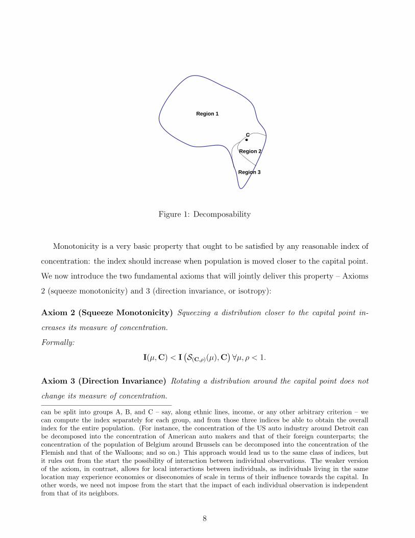
Axiom 1 (Decomposability) The concentration measure of the sum of two distributions with
disjoint supports is the sum of the concentration measures of each distribution.
Formally:
I(µ+ ν,C) = I(µ,C) + I(ν,C)∀µ, ν, Support(µ) ∩ Support(ν) = ∅. (1)
This axiom means that the measure of concentration of a distribution can be (additively) de-
composed into the measures of concentration of its subdistributions defined over non-overlapping
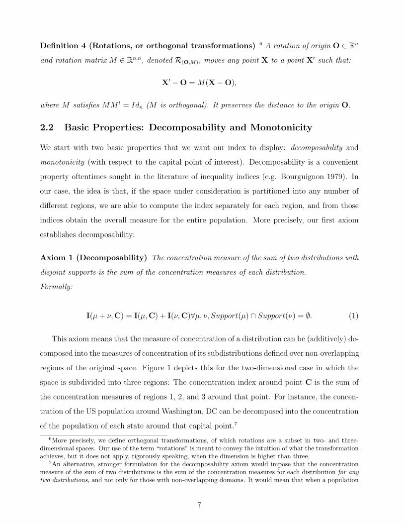
regions of the original space. Figure 1 depicts this for the two-dimensional case in which the
space is subdivided into three regions: The concentration index around point C is the sum of
the concentration measures of regions 1, 2, and 3 around that point. For instance, the concen-
tration of the US population around Washington, DC can be decomposed into the concentration
of the population of each state around that capital point.7
6More precisely, we define orthogonal transformations, of which rotations are a subset in two- and three-dimensional spaces. Our use of the term “rotations” is meant to convey the intuition of what the transformationachieves, but it does not apply, rigorously speaking, when the dimension is higher than three.
7An alternative, stronger formulation for the decomposability axiom would impose that the concentrationmeasure of the sum of two distributions is the sum of the concentration measures for each distribution for anytwo distributions, and not only for those with non-overlapping domains. It would mean that when a population
7
C
Region 2
Region 1
Region 3
Figure 1: Decomposability
Monotonicity is a very basic property that ought to be satisfied by any reasonable index of
concentration: the index should increase when population is moved closer to the capital point.
We now introduce the two fundamental axioms that will jointly deliver this property – Axioms
2 (squeeze monotonicity) and 3 (direction invariance, or isotropy):
Axiom 2 (Squeeze Monotonicity) Squeezing a distribution closer to the capital point in-
creases its measure of concentration.
Formally:
I(µ,C) < I(S(C,ρ)(µ),C
)∀µ, ρ < 1.
Axiom 3 (Direction Invariance) Rotating a distribution around the capital point does not
change its measure of concentration.
can be split into groups A, B, and C – say, along ethnic lines, income, or any other arbitrary criterion – wecan compute the index separately for each group, and from those three indices be able to obtain the overallindex for the entire population. (For instance, the concentration of the US auto industry around Detroit canbe decomposed into the concentration of American auto makers and that of their foreign counterparts; theconcentration of the population of Belgium around Brussels can be decomposed into the concentration of theFlemish and that of the Walloons; and so on.) This approach would lead us to the same class of indices, butit rules out from the start the possibility of interaction between individual observations. The weaker versionof the axiom, in contrast, allows for local interactions between individuals, as individuals living in the samelocation may experience economies or diseconomies of scale in terms of their influence towards the capital. Inother words, we need not impose from the start that the impact of each individual observation is independentfrom that of its neighbors.
8

Formally:
I(µ,C) = I(R(O,θ)(µ),C
)∀µ.
To illustrate the implications of these axioms, let us consider the population of a country
and how it is distributed over the country’s territory. Axiom 2 implies that, if the entire
population moves closer to the capital by a given proportion, say one half, then concentration
must increase. However, it applies only to moves along the respective rays going through the
capital and the original locations. (This is depicted, in two dimensions, in Figure 2.) Axiom
3, on the other hand, means that if the entire population of a country moves 20 miles to the
right, while keeping everyone’s initial distance to the capital unchanged, then concentration
must remain constant. In other words, the direction from the capital city to each location
is irrelevant to concentration. (This is depicted in Figure 3.)8 Taken together, these two
axioms mean that a movement that brings the population closer to the capital point, along any
direction, must increase concentration, while it must decrease concentration if the population
is moved farther away from the capital city. In other words, they deliver monotonicity with
respect to the capital.
Note that here the convenience of the decomposability property delivered by Axiom 1 comes
to the forefront: it means that Axioms 2 and 3 can be understood in terms of the movements
of individuals in the population, which can enhance the intuition behind them. Axiom 2 means
that, if we take a specific individual in the population who lives, say, 200 miles away from the
capital city, then if she moves to live some 10 miles towards the capital city, concentration
should increase. Axiom 3 in turn guarantees that, if that individual moves to another place
of equal distance (200 miles) to the capital city, then concentration should not change, or in
other words, the direction from the capital city to each individual’s location is irrelevant to
concentration. The two axioms together mean that if an individual moves closer to the capital,
along any direction, then concentration must increase.
These three basic axioms already have a powerful implication, as shown in Proposition
1. To understand this proposition, let us first introduce some notation for the impact of an
8In certain realistic cases, one could argue that not all directions are equal – say, because of the presence of aroad that makes it easier to move in some direction, or of a mountain that makes it harder to move in another.However, this concern does not invalidate our framework, as one could rescale the dimensions accordingly.Further discussion on such conditions will follow later in the text, but this highlights the advantages of workingwith general and abstract Euclidian spaces.
9

C
Figure 2: Squeeze Monotonicity
C
Figure 3: Rotation Invariance
10

individual at location x on the capital C, by defining the impact function h of the locations x,
C. Proposition 1 then states that the CISC must be the (integral) sum of the impacts of each
individual observation, and that the impact of each individual must be expressed as a function
of solely the distance to the capital point of interest, i.e. h(|x − C|). In addition, it must be
the case that h(d) is decreasing in d. More formally:
Proposition 1 Axioms 1, 2 and 3 define the following class of population concentration in-
dices:
I(µ,C) =
∫h(|x−C|)dµ, (2)
with h(d) being a decreasing function on R+ so that the right hand side’s integrand is integrable
on Rn.
Proof of Proposition 1. See Appendix.
This proposition establishes two separate properties. The first is additivity : the CISC is the
sum of the impacts of individual observations. The proof of the proposition shows that this is
directly related to Axiom 1. The second property, that the impact function is a (decreasing)
function of distance only, is clearly related to the property of monotonicity that is delivered by
Axioms 2 and 3.9 Finally, Proposition 1 also makes clear that normalization, or multiplication
of the population distribution µ of a factor k will change the CISC by exactly the same factor.
This enables us to disentangle concentration from population size; in other words, it justifies
our focus on normalized distributions, i.e. µ such that∫µ = 1, without loss of generality.
2.3 Refinement: Order Preservation, Convexity and Local Mono-tonicity
Proposition 1 shows that the first three axioms impose non-trivial restrictions on the class of
admissible indices. However, it still leaves us with a fairly large class. After all, any decreasing
function of the distance between individual points and the center C would be an admissible
impact function h(d): a few obvious suggestions of standard functional forms include a step
function, and logarithmic, exponential or polynomial (including linear) functions, among others.
9The three axioms interact closely in implying that the impact function, which from Axiom 1 alone could bedefined in general as a function of the locations x, C, and also the local population density µ(x), can be definedsimply as a function h(x,C).
11
In this section we will introduce three natural properties that would drastically restrict this
class of indices into a very manipulable set of measures.
2.3.1 Order Preservation: Isoelasticity
Let us start by considering a property that has to do with what happens when we change the
units in which distances are measured. Suppose we have two distributions, (µ,C), and (ν,C),
and the distances between points are measured in miles. If µ is deemed to be more concentrated
around C than ν, it stands to reason that this relative ranking should not change if distances
were instead measured in kilometers. In other words, changing the unit of distance measure
should not change the ordering of distributions by the CISC. This change in units is isomorphic
to a squeeze of the distribution around the capital point of interest by a factor of ρ, where ρ > 0
gives us the conversion rate between the different units. (Obviously, a “squeeze” in which ρ > 1
is actually an expansion around the capital point.) As a result, our property affirms that the
relative order of different distributions remains unchanged when they are squeezed or expanded
around the capital.
Axiom 4 (Order Preservation) The ordering of two distributions of equal population by
their CISC is not changed after re-scaling measures of distance.
Formally: Given two distributions µ and ν of the same total mass (∫dµ =
∫dν), if I(µ,C) ≥
I(ν,C), then I(S(C,ρ)(µ),C) ≥ I(S(C,ρ)(ν),C),∀ρ > 0.
As it turns out, adding this very natural axiom to the previous three has powerful implica-
tions in terms of pinning down a class of admissible CISCs. More precisely, Axiom 4 defines
a specific subclass of impact functions within the class defined by Proposition 1 – it is that of
isoelastic impact functions, as stated in the following Proposition:
Proposition 2 (Isoelasticity) Axiom 4 and Proposition 1 imply that the impact function
must be isoelastic (constant relative risk aversion), i.e. that it is h(d) ≡ αdγ + β or h(d) ≡
α log(d) + β.
Proof of Proposition 2. See Appendix.
In other words, if we define Rh(d)def≡ −h′′(d)d
h′(d), the elasticity of the marginal impact function
with respect to distance10 – or alternatively, the “coefficient of relative risk aversion” of the
10Technically, Proposition 2 also affirms the infinite differentiability of the impact function h, so the expressionof Rh(d) is meaningful.
12
impact function – then Proposition 2 establishes that our class of admissible CISCs must have
Rh(d) = Rh, a constant. (Obviously, we have Rh = 1− γ, and the log function is the limit case
when γ → 0.)
2.3.2 Convexity and Local Monotonicity: Boundary Restrictions
The class of admissible indices is further restricted by considering two additional properties
that a CISC should display. The first property takes a movement akin to the one considered in
Axiom 2, bringing an individual observation closer to the capital along the ray going through
her initial location, and asks what happens when we vary the initial point of this movement.
In other words, if we move an individual 10 miles closer to the capital, does it matter whether
she started 20 or 200 miles away? Or, to take a concrete example, if we want to measure the
concentration of Russia’s population around Moscow, should a given movement of individuals
matter more or less whether it happens in the outskirts of Moscow or in Vladivostok in the
far east corner of the country? It seems natural to assume that the former case should matter
more than the latter. We thus posit that the marginal movement is (at least weakly) more
important when the individual is close to the capital than when she is far away – that is to say,
as an individual moves towards the center, not only her level of impact, but also her marginal
impact on concentration is not decreasing. This requirement can be written as follows:
Axiom 5 (Convexity) The marginal change in the impact of an individual is not increasing
in his distance to the center.
Formally:
h′′(d) ≥ 0.
We also impose restrictions on how the index behaves with respect to any other point in the
space, besides the capital. Our next property has to do with changes of the index in response
to squeezes of the distribution around any arbitrary point in the space, not restricted to the
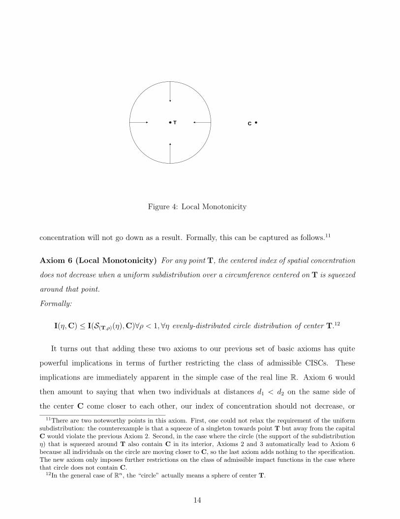
capital. Consider individual observations that are uniformly distributed around a given point
T . Similar to Axiom 2, we posit that our index of concentration should not decrease when those
individual observations are squeezed together around a given point T , as depicted in Figure
4. The intuitive idea is that, if individuals move closer to each other, we would expect that
13
T C
Figure 4: Local Monotonicity
concentration will not go down as a result. Formally, this can be captured as follows.11
Axiom 6 (Local Monotonicity) For any point T, the centered index of spatial concentration
does not decrease when a uniform subdistribution over a circumference centered on T is squeezed
around that point.
Formally:
I(η,C) ≤ I(S(T,ρ)(η),C)∀ρ < 1,∀η evenly-distributed circle distribution of center T.12
It turns out that adding these two axioms to our previous set of basic axioms has quite
powerful implications in terms of further restricting the class of admissible CISCs. These
implications are immediately apparent in the simple case of the real line R. Axiom 6 would
then amount to saying that when two individuals at distances d1 < d2 on the same side of
the center C come closer to each other, our index of concentration should not decrease, or
11There are two noteworthy points in this axiom. First, one could not relax the requirement of the uniformsubdistribution: the counterexample is that a squeeze of a singleton towards point T but away from the capitalC would violate the previous Axiom 2. Second, in the case where the circle (the support of the subdistributionη) that is squeezed around T also contain C in its interior, Axioms 2 and 3 automatically lead to Axiom 6because all individuals on the circle are moving closer to C, so the last axiom adds nothing to the specification.The new axiom only imposes further restrictions on the class of admissible impact functions in the case wherethat circle does not contain C.
12In the general case of Rn, the “circle” actually means a sphere of center T.
14
equivalently, that 0 ≥ h′(d1) ≥ h′(d2). Yet Axiom 5 implies that h′(d1) ≤ h′(d2) ≤ 0. Thus
h′(d) is constant, i.e. the impact function h must be linear: h(d) = αd + β, α < 0. We have
thus pinned down a unique class of admissible CISC, with a linear impact function, for the
special case of the real line.
Our axiomatic approach enables us to be much more general. Quite remarkably, we can
show (using harmonic function theory) that the basic intuition of the one-dimensional case
extends to any n-dimensional Euclidian space, as our Axioms 5 and 6 define a specific subclass
of impact functions within the class defined by Proposition 1:
Proposition 3 (Boundary Restrictions) Within the class of centered indices of spatial con-
centration on Rn defined in Proposition 1, Axioms 5 and 6 determine the following subclass of
indices:
I(µ,C) =
∫h(|x−C|)dµ, (3)
with h(d) being a decreasing function of distance and 0 ≤ Rh(d) ≤ n−1, where Rh(d)def≡ −h′′(d)d
h′(d).
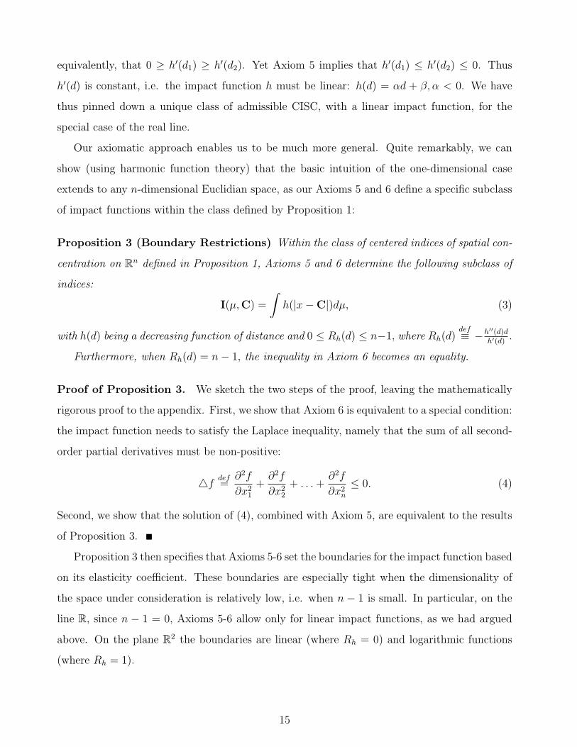
Furthermore, when Rh(d) = n− 1, the inequality in Axiom 6 becomes an equality.
Proof of Proposition 3. We sketch the two steps of the proof, leaving the mathematically
rigorous proof to the appendix. First, we show that Axiom 6 is equivalent to a special condition:
the impact function needs to satisfy the Laplace inequality, namely that the sum of all second-
order partial derivatives must be non-positive:
4f def=
∂2f
∂x21
+∂2f
∂x22
+ . . .+∂2f
∂x2n
≤ 0. (4)
Second, we show that the solution of (4), combined with Axiom 5, are equivalent to the results
of Proposition 3.
Proposition 3 then specifies that Axioms 5-6 set the boundaries for the impact function based
on its elasticity coefficient. These boundaries are especially tight when the dimensionality of
the space under consideration is relatively low, i.e. when n − 1 is small. In particular, on the
line R, since n − 1 = 0, Axioms 5-6 allow only for linear impact functions, as we had argued
above. On the plane R2 the boundaries are linear (where Rh = 0) and logarithmic functions
(where Rh = 1).
15
2.4 Characterization of the Class of Admissible CISCs
We are now ready to characterize our class of admissible CISCs. Proposition 1 establishes that
an index that satisfies decomposability and monotonicity has to be represented by the sum of
the impacts of individual observations, which are in turn captured by an impact function that
is a (decreasing) function of the distance to the capital point of interest only. Propositions 2
and 3 then establish that the key element of that impact function is Rh(d), which describes the
elasticity of the marginal impact of individual observations with respect to their distance from
the capital point. An index that satisfies order preservation must have a constant elasticity
(Proposition 2), and an index that satisfies convexity and local monotonicity must have that
elasticity bounded between zero and an upper limit dependent on the dimensionality of the space
under consideration (Proposition 3). When we combine the three propositions, we immediately
obtain the following Characterization Theorem:
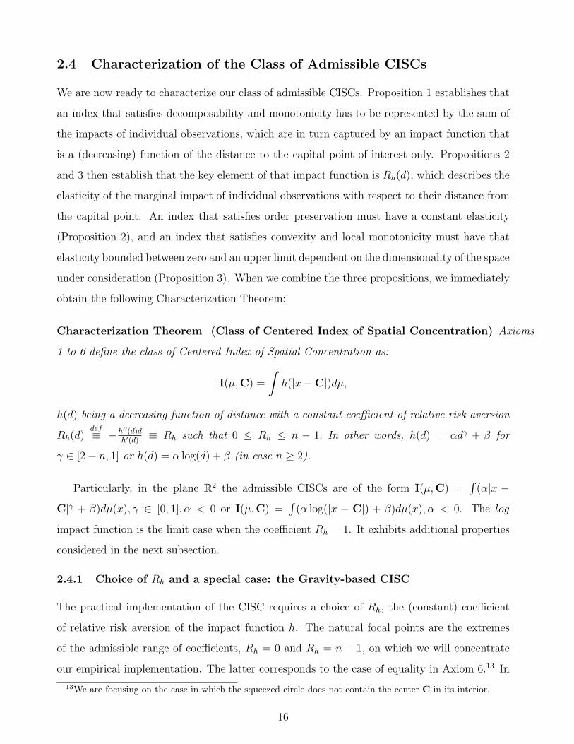
Characterization Theorem (Class of Centered Index of Spatial Concentration) Axioms
1 to 6 define the class of Centered Index of Spatial Concentration as:
I(µ,C) =
∫h(|x−C|)dµ,
h(d) being a decreasing function of distance with a constant coefficient of relative risk aversion
Rh(d)def≡ −h′′(d)d
h′(d)≡ Rh such that 0 ≤ Rh ≤ n − 1. In other words, h(d) = αdγ + β for
γ ∈ [2− n, 1] or h(d) = α log(d) + β (in case n ≥ 2).
Particularly, in the plane R2 the admissible CISCs are of the form I(µ,C) =∫
(α|x −
C|γ + β)dµ(x), γ ∈ [0, 1], α < 0 or I(µ,C) =∫
(α log(|x − C|) + β)dµ(x), α < 0. The log
impact function is the limit case when the coefficient Rh = 1. It exhibits additional properties
considered in the next subsection.
2.4.1 Choice of Rh and a special case: the Gravity-based CISC
The practical implementation of the CISC requires a choice of Rh, the (constant) coefficient
of relative risk aversion of the impact function h. The natural focal points are the extremes
of the admissible range of coefficients, Rh = 0 and Rh = n − 1, on which we will concentrate
our empirical implementation. The latter corresponds to the case of equality in Axiom 6.13 In
13We are focusing on the case in which the squeezed circle does not contain the center C in its interior.
16

other words, any local force of concentration at an arbitrary point T that moves people situated
evenly on a circle around T towards it does not affect the global measure of concentration
around C. The index thus measures the “gravitational pull” exerted by the capital point, while
disentangling from the data any impact of the presence of other local forces. It is invariant
to changes in the degree of attraction, or “gravity”, of any other points. An analogy comes
from the gravitational pull of the Sun over the Earth, which is measured focusing only on the
distance between the two bodies and their characteristics (mass), leaving aside the influence of
all other planets.14 We define this “Gravity-based CISC” (G-CISC) as follows.
Property 1 (Gravity) For any point T, the CISC does not change when a uniform subdis-
tribution over a circumference centered on T is squeezed around that point.
Proposition 4 (The Gravity-based CISC) Axioms 1-3 and Property 1 pin down the Gravity-
based CISC, or G-CISC, with the following impact function:
h(d) =
αd+ β ∀d > 0, α < 0 if n = 1α log d+ β ∀d > 0, α < 0 if n = 2αd2−n + β ∀d > 0, α > 0 if n ≥ 3
.
Proof of Proposition 4. Immediately follows from the Characterizaton Theorem.
Robustness to Measurement Errors The G-CISC brings an additional property that
is very convenient in applications. In practice, the information used to compute the index
typically comes in a grid format, where we only know the aggregate information of each cell.
This introduces a source of measurement error. The G-CISC is orthogonal to such measurement
error, thanks to the Property of Gravity. Indeed, if the population is symmetrically distributed
within each cell, the Property of Gravity implies that we could replace that population with
one mass point at the center.
14The analogy with gravity is actually deeper than what might seem at first sight: there is a connectionbetween the G-CISC and the concept of potential in physics, which refers to the potential energy stored withina physical system – e.g. gravitational potential is the stored energy that results in forces that could move objectsin space. In fact, our G-CISC can be interpreted, roughly speaking, as a measure of the potential associated withthe capital point of interest. This is because the G-CISC is the index that satisfies the Laplace equation, whichis stated as an inequality in the proof of Proposition 3, and potential is defined by a solution to that equation –those readers familiar with the physics of the concept will have noticed the connection from the use of harmonicfunction theory. To see this connection more clearly, note that in the “real life” three-dimensional space ofNewtonian mechanics, the potential of a point with respect to a mass is the sum of inverse distances from thatpoint to each location in the mass – and since the gravity force is the derivative of potential, it is proportionalto the inverse of the squared distance, as one may recall from the classical Newtonian representation. OurG-CISC in three-dimensional space is also the weighted sum of the inverse of distance, and thus coincides withthe concept of potential in physics.
17
2.5 Normalization
A crucial feature of the CISC defined in the Characterization Theorem is its flexibility: as long
as it is applied to a distribution µ that is defined over a Euclidian space of any dimension,
its desirable properties are ensured. This flexibility means that in any application it will be
possible to shape the index in order to make it most suitable to the specific goals of the analysis.
This can be done both by conveniently redefining the distribution under analysis, as we had
indicated by focusing on normalized, unit-size distributions in our theoretical discussion, and
by making use of the degrees of freedom afforded by the Characterization Theorem with regard
to the choice of parameters α and β.
In order to see this more clearly, and motivated by our empirical implementation, let us fix
ideas by focusing on a situation where our index is applied to the concentration of the population
of a given geographic unit of analysis (e.g. a country) around a point of interest (e.g. the capital
city), in two dimensions. Furthermore, we start by focusing our interest on the special case
of the G-CISC – which means that the impact function is given by h(d) = α log(d) + β. (It
is straightforward to extend the following analysis to other contexts.) In this context, we can
think of any given country as a centered distribution (µ,C). The first thing to note is that
there is often other information, in addition to population size, that we may want to disentangle
from population concentration per se, e.g. the geographical size of the country. In addition,
we would like to have an easily interpretable scale. A convenient way would be to restrict the
index to the [0, 1] interval, with 0 and 1 representing situations of minimum and maximum
concentration, respectively. The latter can be defined simply as a situation in which the entire
population is located in the center of interest; the former is a case in which it is located as far
from the center as possible, where “as far as possible” is suitably defined.
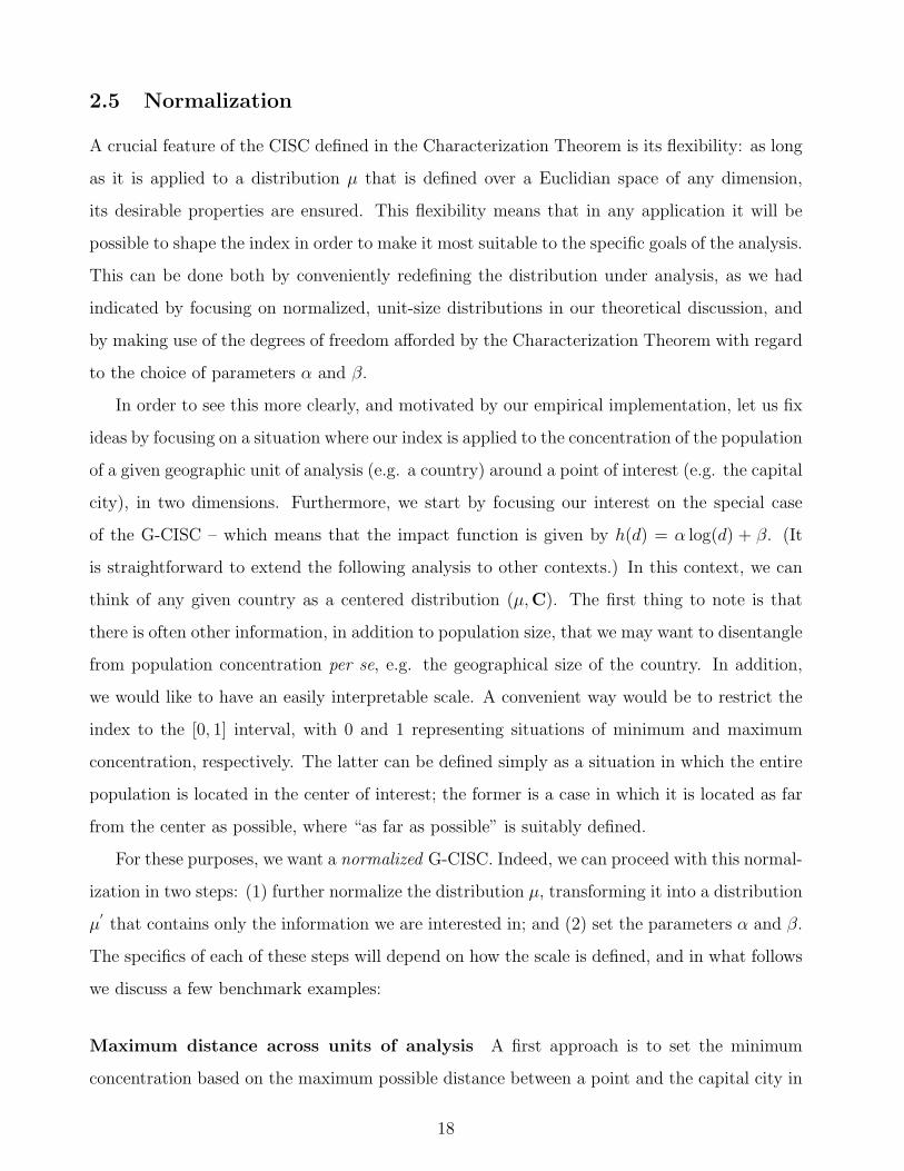
For these purposes, we want a normalized G-CISC. Indeed, we can proceed with this normal-
ization in two steps: (1) further normalize the distribution µ, transforming it into a distribution
µ′
that contains only the information we are interested in; and (2) set the parameters α and β.
The specifics of each of these steps will depend on how the scale is defined, and in what follows
we discuss a few benchmark examples:
Maximum distance across units of analysis A first approach is to set the minimum
concentration based on the maximum possible distance between a point and the capital city in
18
any of the countries for which the index is to be computed. In this case, the index is evaluated
at zero if the entire population lives as far away from the center as it is possible to live in any
country.15 (As a result, only one country, the one where this maximum distance is registered,
could conceivably display an index equal to zero.) This will be appropriate if we want to
compare each country’s concentration against a single benchmark.
In order to achieve this, the two steps are:
1. The standard normalization of the distribution to separate population size from concen-
tration is sufficient here: Normalize the distribution by dividing µ by population size,∫dµ, which means that we will be taking each country to have a population of size one.
2. Set:
(α, β) =
(− 1
log(d), 1
)where d ≡ maxxi,i |xi −Ci| is the maximum distance between a point and the center in
any country. This means that we take the (logarithm of the) largest distance between a
point and the capital in any country to equal to one.
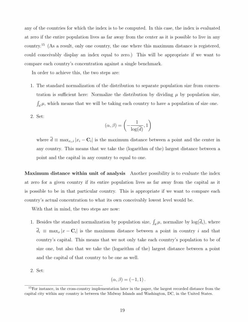
Maximum distance within unit of analysis Another possibility is to evaluate the index
at zero for a given country if its entire population lives as far away from the capital as it
is possible to be in that particular country. This is appropriate if we want to compare each
country’s actual concentration to what its own conceivably lowest level would be.
With that in mind, the two steps are now:
1. Besides the standard normalization by population size,∫dµ, normalize by log(di), where
di ≡ maxx |x−Ci| is the maximum distance between a point in country i and that
country’s capital. This means that we not only take each country’s population to be of
size one, but also that we take the (logarithm of the) largest distance between a point
and the capital of that country to be one as well.
2. Set:
(α, β) = (−1, 1) .
15For instance, in the cross-country implementation later in the paper, the largest recorded distance from thecapital city within any country is between the Midway Islands and Washington, DC, in the United States.
19

Our empirical implementation will illustrate both cases of normalization and their different
interpretations.
2.6 Comparison with Other Indices
Comparison with other Centered Indices The first obvious comparison is to other cen-
tered indices of spatial concentration used in the literature. Some widely used measures of
spatial concentration discard a lot of information, by attaching zero weight to observations
located at more than a certain distance from the capital point. One such example of partic-
ularly stark nature is the share of individual observations that is right on the capital point; a
typical application of such a measure is the share of population of a country that lives in the
capital city, or in the main city in that country, as in Ades and Glaeser (1995). The obvious
advantage of our approach is that it incorporates all of that information, with enough flexibility
to allow for different weights according to the application – as parameterized by the elasticity
of the marginal impact function with respect to distance (as in Proposition 2): the greater that
elasticity, the less weight is attached to observations that are farther away from the capital
point.
However, other widely used measures also incorporate that information. For instance, Gal-
ster et al. (2001) use the inverse of the sum of the distances of each observation to the center
as a measure of “centrality” in the context of studying urban sprawl. This measure is related
to a limit case in our framework where Rh = 0, i.e. the impact function h is linear, though the
inverse operation used by Galster et al. erases the nice properties of additivity and decompos-
ability. While certainly useful, such ad hoc approaches are limited by what an intuitive grasp
of the properties of a given space will provide. This intuitive grasp quickly reaches its limits
when we move away from specific, concrete applications. Our axiomatic approach, in contrast,
guarantees basic desirable properties for our index in any n-dimensional Euclidian space, which
ensures wide applicability, to any situation that can be mapped onto such a space. Our ap-
proach thus provides a single “language” to codify the concept of spatial concentration around
a capital point. In that sense, our CISC is analogous to the Gini coefficient as a measure of
inequality: it might be less suited than some other measure within a given specific application,
but it has robust properties that make it a good measure across a wide variety of applications,
and as such it provides a universal language to talk about the concept at hand. On the other
20

hand, it still retains considerable flexibility – in that it allows for different coefficients Rh and
different normalization procedures, as described in the previous subsection – that can help us
tailor the index to specific applications, without losing the desirable general properties.
Comparison with Non-Centered Indices of Concentration Besides the obvious distinc-
tion that our index is built on the concept of a particular “center”, it also contains considerably
more spatial information than non-centered indices. For instance, let us consider the many in-
dices of concentration that are based on measures first designed to deal with inequality – such
as the location Gini coefficient calculated on a distribution of cells.16 Such measures do not
take into account the actual spatial distribution. Indeed, consider a thought experiment where
half of the cells contain exactly one individual observation, and the other half contain zero
observations. Such indices do not make any distinction between a situation in which the former
cells are all in the East and all the latter cells are in the West, and another situation in which
both types are completely mingled together in a chess-board pattern. Generally speaking, this
type of measure fails to take into account the relative positions between the cells, which can
be highly problematic in many circumstances.17 In addition, these measures are also highly
non-linear with respect to individuals, because they contain a function of the cell distribution.
In that sense, they are not grounded at the individual level in the way our CISC is.
These differences are highlighted by the fact that we can actually derive a non-centered index
from our centered measure. We can do so by averaging the centric index over all possible centers
(i.e. all points) within the support of the distribution, a feasible task in most applications. On R
(say, applied to individual income distributions), this aggregative, non-centered index coincides
with the much familiar Gini index of inequality. For now, we leave further explorations on this
subject for future work. In any case it is not possible to follow the reverse path and obtain
a centered index from a given non-centered measure. This underscores the versatility of our
approach.
16For instance, the location Gini is used, inter alia, in the context of economic geography (Krugman 1991,Jensen and Kletzer 2005), studies of migration (Rogers and Sweeney 1998), political economy (Collier andHoeffler 2004).
17The same can be said of cruder measures of concentration, such as population density. A related index thatdoes use spatial information is the measure of compactness developed by Fryer and Holden (2007).
21

Comparison with Related Indices: Inequality, Segregation, Polarization, Riskiness
Finally, it is worth noting the links between our index and other indices designed to measure
other aspects of distributions, be they spatial or not. The connection with inequality measures
has already emerged from the very fact that such measures are used to capture spatial concen-
tration, and we have noted that a natural extension of our approach to a non-centered setting
highlights an interesting connection with the Gini coefficient. The connection can be pushed
further when we realize that a Lorenz-curve-type concentration curve could be formed from
spatial distributions: taking the example of population, we can sort individuals according to
the distance from the center within which they are located. These curves could be ranked when
one dominates another, which can be seen along the lines of Proposition 1: if one distribution
“Lorenz”-dominates another, the former’s corresponding index would be higher than the lat-
ter’s, for any functional form of the impact function satisfying the specification of Proposition
1. It is well-known, however, that this order is not complete. In that regard, our index im-
plies a population-weighted measure for a complete ranking of concentration curves, which in
two-dimensional space is based on the log-scale of distance. This connection is exactly akin
to the one emphasized by Echenique and Fryer (2007) with respect to their segregation index:
any index that intends to rank distributions that are not in a Lorenz-dominance relationship
implies choosing a weighting system, and our axioms give us a well-founded reason to prefer one
system to other alternatives. Another analogy could be drawn with the work on polarization
by Duclos, Esteban and Ray (2004) who also provide a particular order of the Lorenz curves
that emphasizes concentration around several “poles” rather than around one unique capital.
Another interesting connection is with the measurement of riskiness. A desirable property
of a measure of riskiness, as spelled out by Aumann and Serrano (2008) is that it respects first-
and second-order stochastic dominance. If we take our distribution to represent the probability
that some individual observation is randomly located at a certain point relative to the capital
point of interest (not unlike the “dartboard” approach in Ellison and Glaeser 1997), we can
take Axioms 2 and 3 to imply that the index respects FOSD. In other words, we can say that a
distribution FOSDs another distribution if, for any distance x from the capital point C, there is
a greater probability of an individual observation locating closer to C than x under the former
than under the latter; Axioms 2 and 3 guarantee that the former distribution will be measured
by the CISC as having greater concentration. We can even go further and state that our Axiom
22
6 captures a generalization of SOSD for Euclidian spaces with dimension greater than 1; it is
clearly equivalent for the case of a unidimensional space.
3 Application: Population Concentration around Capi-
tal Cities
Having established our CISC and discussed its properties, we now move on to illustrate its
applicability in practice. We focus on the distribution of population around capital points of
interest – capital cities across countries and across US states, and the political center (e.g. the
location of city halls) in US metropolitan areas. We will discuss descriptive statistics and basic
correlations with variables of interest, and also how the index can be used to shed light on
competing theories, using as an example the determinants of the location of capital cities.
3.1 Cross-country implementation
In our first application, we calculate population concentration around capital cities across coun-
tries in the world. We use the database Gridded Population of the World (GPW), Version 3
from the Socio-Economic Data Center (SEDC) at Columbia University. This dataset, published
in 2005, contains the information for the years 1990, 1995 and 2000, and is arguably the most
detailed world population map available. Over the course of more than 10 years, these data are
gathered from national censuses and transformed into a global grid of 2.5 arc-minute side cells
(approximately 5km), with data on population for each of the cells in this grid. 18
We present the two limit cases of our CISC in two-dimensional space. The first case, Rh = 1,
is the G-CISC, with the logarithmic impact function, and we compute two different normalized
versions of it. The first version (GCISC1) is normalized by the maximum distance across
countries, and the second version (GCISC2) is normalized by the maximum distance within
the country, both as described in section 2.5: the former captures concentration relative to
what it could possibly be in any country, while the latter captures concentration relative to
what it could possibly be in that specific country.19 The second case, Rh = 0, is the linear
18We limit our analysis to countries with more than one million inhabitants, since most of the examples withextremely high levels of concentration come from small countries and islands. The results with the full sampleare very much similar, however, and are available upon request.
19While the non-normalized measure may present some interest in itself, we do not report it because of itsextremely high correlation with population size, which prevents us from disentangling any independent effect.
23
impact function, which as a short-hand we will call L-CISC. In the interest of brevity, we will
only compute the version normalized by the maximum distance across countries, LCISC1.
We will compare our indices with two alternative measures of concentration. The first
alternative is the location Gini coefficient (“Gini Pop”), a non-centered measure that is often
used in the literature, and the second one is the share of the population living in the capital city
(“Capital Primacy”), which provides a benchmark for comparison with another very simple
centered index.20
3.1.1 Descriptive Statistics
Table 1 shows the basic descriptive statistics for the different measures, for the three years in
the sample, and Table 2 presents their correlation. The first remarkable fact is that there is
very little variation over that span of time: the autocorrelation is extremely high, and almost all
variation comes from the cross-country dimension. This suggests that the pattern of population
distribution is fairly constant within each country, and that a period of 10 years may be too
short to see important changes in that pattern. For this reason, we choose to focus on one of
the years; we choose 1990 because it is the one that has the highest quality of data, as judged
by the SEDC.21
[TABLES 1 AND 2 HERE]
Let us start by comparing the basic properties of our indices with those of the comparison
measures, noting that the appropriate benchmark for comparison in the case of G-CISC is
GCISC1, and not GCISC2, since both location Gini and Capital Primacy do not normalize
by the geographical size of each country. The striking fact that immediately jumps from Table 2
is that our index captures a very different concept from what the location Gini is capturing: they
are negatively correlated, both in the case of G-CISC and L-CISC. This underscores the point
that typical measures of concentration are ill-suited for getting at the idea of concentration
around a given point. This point becomes even more striking when we compare the list of
20We could have included other measures, notably the inverse of the average distance, as used for instance byGalster et al. (2001). We do not do so in the interest of brevity, but it is worth noting that the inverse of theaverage distance is extremely highly correlated with L-CISC, by construction, since the latter also uses averagedistances. In this sense, we can essentially reproduce any results to be obtained with such a measure, but withthe nice properties attached to the CISC.
21Our results are very similar when we use the other two years.
24

countries with very high and very low levels of concentration, which are displayed in Table
3. We can see that the list of the countries whose population is least concentrated around
their capital cities accords very well with what was to be expected: these are by-and-large
countries where the capital city is not the largest city. (The exceptions are Russia, on which
we will elaborate later, and the Democratic Republic of the Congo, formerly Zaire, whose
capital is located on the far west corner of the country.) By the same token, the list of highly
concentrated countries is quite intuitive as well, with Singapore leading the way. The same list
for the location Gini, in contrast, surely helps us understand why the correlation between the
two is negative. It ranks very highly countries that have big territories and unevenly distributed
populations. While this concept of concentration may of course be useful for many applications,
it is quite apparent that using non-centered measures of concentration can be very misleading
if the application calls for a centered notion of concentration.22
[TABLE 3 HERE]
In the case of the alternative centered measure of concentration, Capital Primacy, Table 2
shows that the correlation is positive, though not overwhelming.23 Table 3 shows, however, that
the ranking of countries that emerges from this measure is completely different from the ones
generated by both CISCs.24 This is not surprising, in light of the amount of information that is
being discarded by Capital Primacy, but another crucial problem with such a coarse measure
is clearly apparent from the table: its arbitrariness. Note that Kuwait, which is one of the
most concentrated countries in the world according to both CISCs, shows up as one of the least
concentrated ones as judged by Capital Primacy. This is so because the population of what
is officially considered as Kuwait City, the capital, is just over 30,000, while the population of
the metropolitan area is over two million. This difference of two orders of magnitude is simply
due to an arbitrary delimitation of what counts as the capital city. This clearly illustrates the
dramatic distortions that can result from discarding relevant information.
22It is also worth noting that a measure such as location Gini is quite sensitive to how “coarse” the grid thatis being used to compute the index is: the fewer cells there are, the lower the location Gini will tend to be. Ourindex, on the other hand, has the “unbiasedness” feature that we have already discussed.
23Note also that the maximum value of Capital Primacy is greater than one. This is due to the fact that thedata for capital city population and total population, used to compute the share, come from different sources;that data point corresponds to Singapore, which should obviously be thought of as having a measure of 1.
24Note that here we use the measure of Capital Primacy as computed for 1995. This is because there aremany fewer missing values for 1995 than there are for 1990.
25

We can also compare the two versions of our index, L-CISC and G-CISC, in order to
understand the consequences of changes in the elasticity coefficient. Table 2 shows that the
correlation between GCISC1 and LCISC1 is positive and quite high, which is reassuring since
they both purport to measure the same concept. Nevertheless, there are important empirical
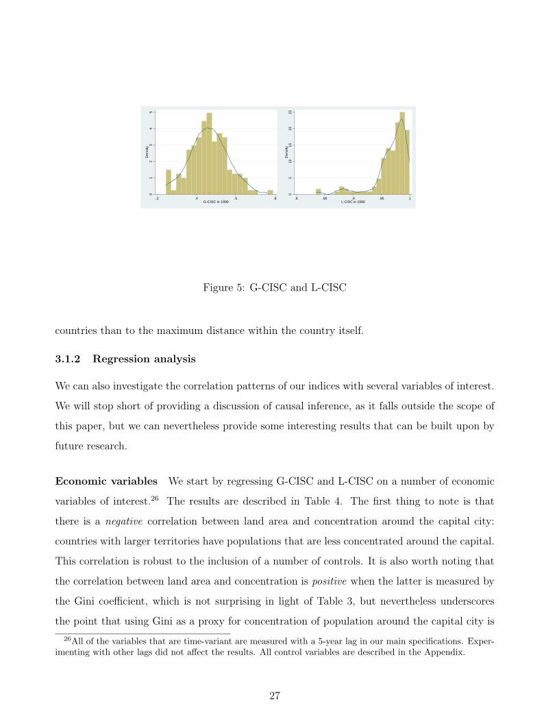
differences between the two. The first such difference can be seen from Figure 5, which plots
histograms of both indices. We can see from the figure that the distribution of LCISC1 is
very skewed, whereas GCISC1 has a more compelling bell-shaped distribution. This implies
that the latter is generally less sensitive to extreme observations. Another way to illustrate
this difference is to consider a specific comparison, between Brazil and Russia. Russia’s capital,
Moscow, is the country’s largest city, and is located at about 600km (slightly less than 400 miles)
from the country’s second largest city, St Petersburg. In contrast, Brazil’s capital, Brasılia, is
now the country’s sixth largest city, and is around 900km (more than 550 miles) away from
the country’s largest cities, Sao Paulo and Rio de Janeiro, whose combined metropolitan area
population is about ten times as large as Brasılia’s.25 Table 3 shows that Brazil is ranked to
have lower concentration than Russia with GCISC1, but not with LCISC1. This is because
LCISC1 gives a larger weight to people who are very far from the capital point of interest;
roughly speaking, it gives a relatively large weight to people who are in Vladivostok. This
example drives home the point that different choices of the elasticity coefficient lead to different
characterizations, thus illustrating the flexibility of our approach.
Finally, we also note an interesting pattern emerging from Table 3, regarding the “size-
normalized” version of our G-CISC, GCISC2: the countries with the most concentrated popu-
lations seem to be fairly small ones (in terms of territory). This does not arise from “mechanical”
reasons, first of all because the measure is normalized for size – the pattern suggests that the
population of relatively small countries is more concentrated than that of large ones, relative
to what it could be. In addition, while the measure for these countries may be less precise
because of the small size, and consequent smaller number of grids, we know that our index is
unbiased to classical measurement error. We will explore this pattern more systematically in
our regression results. We can also note that GCISC1 is typically much higher than GCISC2:
a country will have a more concentrated population relative to the maximum distance across
25According to official data, the metro area population of Sao Paulo, Rio de Janeiro, and Brasılia is around19 million, 12 million, and 3 million, respectively.
26
01
23
45
Den
sity
.2 .4 .6 .8G-CISC in 1990
05
1015
2025
Den
sity
.8 .85 .9 .95 1L-CISC in 1990
Figure 5: G-CISC and L-CISC
countries than to the maximum distance within the country itself.
3.1.2 Regression analysis
We can also investigate the correlation patterns of our indices with several variables of interest.
We will stop short of providing a discussion of causal inference, as it falls outside the scope of
this paper, but we can nevertheless provide some interesting results that can be built upon by
future research.
Economic variables We start by regressing G-CISC and L-CISC on a number of economic
variables of interest.26 The results are described in Table 4. The first thing to note is that
there is a negative correlation between land area and concentration around the capital city:
countries with larger territories have populations that are less concentrated around the capital.
This correlation is robust to the inclusion of a number of controls. It is also worth noting that
the correlation between land area and concentration is positive when the latter is measured by
the Gini coefficient, which is not surprising in light of Table 3, but nevertheless underscores
the point that using Gini as a proxy for concentration of population around the capital city is
26All of the variables that are time-variant are measured with a 5-year lag in our main specifications. Exper-imenting with other lags did not affect the results. All control variables are described in the Appendix.
27

deeply misleading.
[TABLE 4 HERE]
It is not that surprising that the measures that are not normalized for size will indicate a
negative correlation with territorial size. However, our GCISC2 index, which is normalized,
also displays a very significant and robust negative correlation, as anticipated from Table 3,
which suggests that such correlation is more than a mechanical artifact of the construction of
the indices.
The second robust correlation pattern displayed by the different versions of our CISC is as
follows: there is a negative correlation between the size of population, and how concentrated
it is around the capital. In other words, the smaller the country’s population is, the more
concentrated it is around the capital. One can speculate over the reasons behind this negative
correlation; perhaps countries with larger populations are more likely to have other centers of
attraction that lead to the equilibrium distribution of population being more dispersed around
the capital city. (We should note, however, that in the case of G-CISC the Property of Gravity,
which isolates the attraction exerted by the capital point of interest, ensures that the existence
of other centers of attraction will not be mechanically built into the index.) It is worth noting
that the relationship is weaker for GCISC2, where concentration is normalized by the territorial
size of the country. These patterns can and should be the subject of future research.27
Governance variables We have argued elsewhere (Campante and Do 2007) that population
concentration is an important determinant of redistributive pressures, particularly so in non-
democratic countries. The basic idea, as expressed in Ades and Glaeser (1995), is that proximity
to the capital city increases an individual’s political influence. This is particularly the case
with regard to “non-institutional” channels like demonstrations, insurgencies and revolutions,
as opposed to democratic elections. As such, a more concentrated population is more capable
of keeping a non-democratic government in check. With that idea in the background, we study
the correlation between our measures of concentration and a number of measures of the quality
27One tentative way of probing deeper into this link with population size is to consider the effects of openness.Introducing openness into the regression reduces the coefficient and significance of population size, which mayindicate that part of the negative relationship is indeed linked to the relative attraction of the capital city, whichmay be more pronounced in a more open, outward-oriented economy. The high correlation between opennessand population makes it hard to disentangle their effects, however.
28

of governance, compiled by Kaufman, Kraay and Mastruzzi (2006). These results are featured
in Table 5.
[TABLE 5 HERE]
The first panel, for the full sample, suggests that there is a positive correlation between
population concentration and governance (with the exception of political stability). The more
striking pattern emerges, however, when we split the sample between democracies and non-
democracies: it is clear that this relationship is present only in non-democratic countries. In this
sub-sample, a higher degree of concentration around the capital city predicts higher governance
quality as measured by five of the six variables – control of corruption, voice and accountability,
government effectiveness, rule of law, and quality of regulation – with an increase of around
30% of standard deviation for an increase of one standard deviation in G-CISC. Essentially no
effect is verified for more democratic countries. This is precisely in line with the idea that the
concentration of population represents a check on non-democratic governments.
The fact that political stability is the one measure of quality of governance that does not
seem to be positively correlated with population concentration is interesting in and of itself. In
fact, if we include the other governance variables as controls in a regression with stability as the
dependent variable, we see that population concentration has a negative and typically significant
correlation with stability – both for G-CISC and L-CISC. Moreover, this result is once again
verified only for non-democratic countries. This is consistent with the idea that, controlling for
the quality of governance in non-democratic polities, the concentration of population around
the capital city imposes checks on the incumbent government.28
Table 5 already shows that the significance of the coefficients is generally improved with
G-CISC, as opposed to L-CISC. This is not too surprising, in light of the more well-behaved
distribution displayed by the former. In fact, we can further establish this comparison, while
also considering how our measures of concentration fare when compared to the alternative
measures we have been using as benchmarks. For that purpose, we run a “horse race” in which
the measures are jointly included, as shown in Table 6 – for brevity, we only present one of the
28These results, which are available upon request, are verified both when stability is measured by the Kaufman,Kraay and Mastruzzi (2006) index, and also when it is measured by the average length of tenure experiencedby incumbent executives or parties in the previous twenty years. For details on this measure, see Campante,Chor, and Do (2009).
29

governance measures, namely control of corruption, and focus on the sample of non-democratic
countries. It is clear that both G-CISC and L-CISC dominate the alternative measures, and
that G-CISC seems to provide the clearest picture of the correlations linking the concentration
of population around the capital city and governance.29
[TABLE 6 HERE]
3.1.3 Where to Locate the Capital?
The idea that the capital city is a particularly important point from a political standpoint, and
the correlation between the concentration of population around the capital and the extent of the
checks on the government suggest that governments – and non-democratic ones in particular
– would have an incentive to pick suitable locations for their capital. This draws attention to
the endogeneity of the location of the capital city: not only is the concentration of population
a variable that is determined in equilibrium, but the concentration patterns can also influence
the choice of where to locate the capital. This is another idea that this application of our index
enables us to address.
While a full treatment of the different avenues of causality is beyond the scope of this paper,
we can nevertheless illustrate how our index can shed light on this topic. More generally, we can
illustrate how our index helps approach the issue of the choice of the capital point of interest.
Consider a country with a given spatial distribution of its population, and let us think of the
problem faced by a ruler with respect to where to locate the country’s capital.30 There are
centripetal forces that would lead the ruler to consider spots where the concentration would
be very high – economies of agglomeration, broadly speaking. But there are other centrifugal
forces, such as the aforementioned checks on his power, that would lead him to place the capital
in a low-concentration spot. The question is, which of these forces will prevail under which
circumstances?
Our index can provide an avenue for answering this question, which we illustrate using
G-CISC. For every country, we compute the concentration of population around every single
point in that country.31 We then specify the point where this concentration reaches its maxi-
29One can once again note that the location Gini goes in the opposite direction of the centered measures.30The history of changes in the location of capital cities, considered at some length in Campante and Do
(2007), is proof that this problem is very often explicitly considered.31More precisely, every single cell in the grid that covers the country.
30

mum value. Interestingly, for three fourths of the countries (in the year 1990) this maximum-
concentration location lies right within the capital city. This high rate is explained in part by
the choice to put the capital in a central location, and in part by the fact that being the capital
increases the location’s attractiveness to migrants and to economic activity in general. More
broadly, the maximum-concentration location is often at the largest city.32
We can then measure the gap between this site and the actual capital, as an indicator
of how far a country’s actual choice of capital is from the point that would maximize the
“agglomeration economies”. We regress this distance, normalized by the greatest distance
to any point in the country, on a set of political variables using OLS and Tobit regressions.
The results are presented in Table 7. When we limit ourselves to non-democratic countries,
we see that a higher level of autocracy predicts a greater distance between the capital city
and the concentration-maximizing location. Then when we limit ourselves to non-autocratic
countries, then a higher level of democracy also predicts a greater distance. When combined
together, both variables of autocracy and democracy predict a greater distance: this shows a
type of U-shaped relationship, in which the centrifugal forces are strongest in both extremes
of autocracy and democracy. This pattern is very robust to the inclusion of many dummy
variables, including regional dummies and legal origin dummies. We can speculate that, on the
autocratic side, more autocratic governments have greater incentive and/or ability to insulate
themselves from popular pressure by locating their capital cities in low-concentration spots.
On the democratic side, it is perhaps the case that additional democratic openness will lead to
greater decentralization, and a lower level of attraction exerted by the capital. We are far from
having a theory to fully account for that at this point, but the stylized fact is quite interesting
nonetheless, and we also leave it to future research.
[TABLE 7 HERE]
3.2 US State-level Implementation
Building on the previous section’s discussion on the location of the capital city, there is no
better country in which to take our empirical implementation to the regional level than the
32The exceptions are often illustrative. In China, it is close to Zhengzhou, the largest city in the province ofHenan, which is the country’s most populous; in India, similarly, it is in the state of Uttar Pradesh, which is alsothe most populous. In the US, it is Columbus, OH, right in the middle of the large population concentrationsof the East Coast and the Midwest.
31

United States, with its long tradition of dealing with the issue. Most famously, James Madison
elaborated at length on the choice of the site of the capital city, during the 1789 Constitutional
convention, arguing that one should “place the government in that spot which will be least
removed from every part of the empire,” and that “regard was also to be paid to the centre [sic]
of population.” He also pointed out that state capitals had sometimes been placed in “eccentric
places,” and that in those cases “we have seen the people struggling to place it where it ought
to be.”33
The force identified by Madison have been very much at play in the case of US states, and
our index enables us to get a snapshot of what the outcome has been. Regarding concentration
normalized by the size of the territory (GCISC2), shown in Table 8, Illinois is less concentrated
around its capital Springfield than any country in the world. Even with country size, its level
of concentration is still comparable with Canada, ranking 10 in the world. Not only for Illinois,
but many US States where the capital is not the largest city have the level of concentration
comparable to the least concentrated countries in the world. On the other hand, the amount of
variation is comparable to that of the cross-country implementation, as states such as Rhode
Island and Hawaii have levels of concentration that on a par with some of the most concentrated
countries in the world. In general, the broad lessons obtained at the cross-country level persist:
GCISC1 and LCISC1 generate similar rankings, and the Gini captures a completely different
concept.
[TABLE 8 HERE]
3.3 US Metropolitan Area Implementation
Finally, for the sake of completeness, we implement our indices in the context of US metropolitan
areas. There is a large literature discussing and measuring urban sprawl in this context, to which
we obviously will not do justice. In any event, the concept of sprawl is multidimensional, and
many different measures have been used to capture these multiple elements (Galster et al. 2001,
Glaeser and Kahn 2003). Our measure of spatial concentration captures what Galster et al.
(2001) call “centrality”, and following that paper we compute our indices taking city hall as
our capital point of interest. The results for 24 major metropolitan areas are in Table 9.
33These quotations were obtained from the website The Founders’ Constitution (on Article 1, Section 8,Clause 17), available at http://press-pubs.uchicago.edu/founders/.
32

[TABLE 9 HERE]
Some of the results are expected – the high levels of concentration in places such as Boston
and New York – while others may be somewhat more surprising to the naked eye – such as
the middling levels of concentration in Los Angeles, a city that is synonymous with urban
sprawl, or perhaps the extremely low level of concentration in San Francisco.34 From a broader
perspective, perhaps the most notable feature is how closely linked are the rankings for the
three versions of CISC, and how numerically close are GCISC1 and GCISC2 compared to the
country- and state-level contexts. The message is simple: when distances are relatively small,
as they are bound to be for cities when compared to countries or states, differences in elasticity
coefficients or normalization procedures are less important.35
4 Concluding Remarks
We have presented a general, axiomatic approach to building a centered measure of spatial
concentration. We show that requiring a few basic properties, meant to be robust across a
variety of applications, enables us to pin down a specific class of measures, defined over any
Euclidian space. We then go on to illustrate the empirical implementation of the measure,
and how this implementation highlights some of the advantages of our index over alternative
approaches.
We emphasize that our approach is a very general one, and unapologetically so. Our idea
was to build an index that is not model-specific, so that it can provide a common language to
operationalize the concept of centered spatial concentration over a broad scope of applications,
in geographical and also in more abstract spaces. We certainly hope that it can be widely
applied. Empirically, our illustrative implementation also opens up avenues for future research,
as the correlations that we are able to point out between our index and a number of variables
of interest can be exploited further, with particular attention to issues of causality that are left
outside the scope of this paper. An extension of our framework to an aggregate, non-centered
measure of concentration is left to future promising research.
34Both results are very much consistent with the findings in Galster et al. (2001).35It is important to keep in mind that we are talking about relative distances, and not their numerical value:
scale does not matter for the CISC!
33

References
[1] Ades, Alberto F. and Edward L. Glaeser (1995), “Trade and Circuses: Explaining UrbanGiants,” Quarterly Journal of Economics 110: 195-227.
[2] Anderson, James E. and Eric van Wincoop (2003), “Gravity with Gravitas: A Solution tothe Border Puzzle,” American Economic Review 93: 170-192.
[3] Armitage, David H. and Stephen J. Gardiner (2001), Classical Potential Theory. London:Springer-Verlag.
[4] Aumann, Robert J. and Roberto Serrano (2008), “An Economic Index of Riskiness,” Journalof Political Economy, 116: 810-836.
[5] Axler, Sheldon, Paul Bourdon and Wade Ramey (2001), Harmonic Function Theory. NewYork: Springer-Verlag.
[6] Busch, Marc L. and Eric Reinhardt (1999), “Industrial Location and Protection: The Po-litical and Economic Geography of U.S. Nontariff Barriers,” American Journal of PoliticalScience, 43: 1028-1050.
[7] Campante, Filipe R., Davin Chor, and Quoc-Anh Do (2009), “Instability and the Incentivesfor Corruption,” Economics & Politics, forthcoming.
[8] Campante, Filipe R. and Quoc-Anh Do (2007), “Inequality, Redistribution, and Popula-tion,” Harvard University (mimeo).
[9] Center for International Earth Science Information Network (CIESIN), Columbia Uni-versity; and Centro Internacional de Agricultura Tropical (CIAT), (2004), “Grid-ded Population of the World (GPW), Version 3”, Columbia University. Available athttp://beta.sedac.ciesin.columbia.edu/gpw.
[10] Collier, Paul and Anke Hoeffler (2004), “Greed and Grievance in Civil War,” Oxford Eco-nomic Papers, 56: 563-595.
[11] Duclos, Jean-Yves, Joan Esteban, and Debraj Ray (2004), “Polarization: Concepts, Mea-surement, Estimation,” Econometrica 72: 17371772.
[12] Echenique, Federico and Roland G. Fryer, Jr. (2007), “A Measure of Segregation Basedon Social Interactions,” Quarterly Journal of Economics 122: 441-485.
[13] Ellison, Glenn and Edward L. Glaeser (1997), “Geographic Concentration in U.S. Manu-facturing Industries: A Dartboard Approach,” Journal of Political Economy 105: 889-927.
[14] Esteban, Joan and Debraj Ray (1994), “On the Measurement of Polarization,” Economet-rica 62: 819-851.
[15] Fujita, Masahisa, Paul Krugman, and Anthony J. Venables (1999), The Spatial Economy:Cities, Regions, and International Trade. Cambridge, MA: MIT Press.
[16] Galster, George, Roy Hanston, Michael R. Ratcliffe, Harold Wolman, Stephen Coleman,and Jason Freihage (2001), “Wrestling Sprawl to the Ground: Defining and Measuring anElusive Concept,” Housing Policy Debate 12: 681-717.
[17] Glaeser, Edward L. and Matthew Kahn (2004), “Sprawl and Urban Growth”, in V. Hen-derson and J. Thisse (eds.), The Handbook of Regional and Urban Economics, Amsterdam:North Holland.
34

[18] Hidalgo, C. A., B. Klinger, A.-L. Barabasi, and R. Hausmann (2007), “The Product SpaceConditions the Development of Nations,” Science 317: 482-487.
[19] Jensen, J. Bradford and Lori Kletzer (2005), “Tradable Services: Understanding the Scopeand Impact of Services Offshoring,” Brookings Trade Forum, 6: 75-134.
[20] Krugman, Paul R. (1991), Geography and Trade, Cambridge, MA: MIT Press.
[21] Ransford, Thomas (1995), Potential Theory in the Complex Plane. Cambridge, UK andNew York: Press Syndicate of the University of Cambridge.
[22] Rogers, Andrei and Stuart Sweeney (1998), “Measuring the Spatial Focus of MigrationPatterns,” The Professional Geographer, 50: 232-242.
[23] Saff, Edward and Vilmos Totik (1997), Logarithmic Potentials with External Fields. Berlin:Springer-Verlag.
35
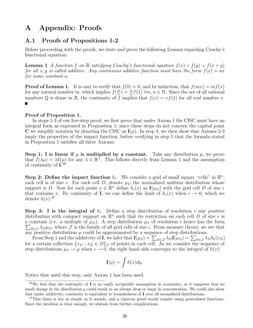
A Appendix: Proofs
A.1 Proofs of Propositions 1-2
Before proceeding with the proofs, we state and prove the following Lemma regarding Cauchy’sfunctional equation:
Lemma 1 A function f on R satisfying Cauchy’s functional equation f(x) + f(y) = f(x+ y)for all x, y is called additive. Any continuous additive function must have the form f(x) = axfor some constant a.
Proof of Lemma 1. It is easy to verify that f(0) = 0, and by induction, that f(mx) = mf(x)for any natural number m, which implies f(m
n) = m
nf(1) ∀m,n ∈ N. Since the set of all rational
numbers Q is dense in R, the continuity of f implies that f(x) = xf(1) for all real number x.
Proof of Proposition 1.In steps 1-3 of our five-step proof, we first prove that under Axiom 1 the CISC must have an
integral form as expressed in Proposition 1; since these steps do not concern the capital pointC we simplify notation by denoting the CISC as I(µ). In step 4, we then show that Axioms 2-3imply the properties of the impact function, before verifying in step 5 that the formula statedin Proposition 1 satisfies all three Axioms.
Step 1: I is linear if µ is multiplied by a constant. Take any distribution µ, we provethat I(λµ) = λI(µ) for any λ ∈ R+. This follows directly from Lemma 1 and the assumptionof continuity of I.36
Step 2: Define the impact function h. We consider a grid of small square “cells” in Rn,each cell is of size ε. For each cell D, denote µD the normalized uniform distribution whosesupport is D. Now for each point x ∈ Rn define hε(x) as I(µD) with the grid cell D of size εthat contains x. By continuity of I, we can define the limit of hε(x) when ε → 0, which wedenote h(x).37
Step 3: I is the integral of h. Define a step distribution of resolution ε any positivedistribution with compact support on Rn such that its restriction on each cell D of size ε isa constant (i.e. a multiple of µD). A step distribution µS of resolution ε hence has the form∑
D∈J λDµD, where J is the family of all grid cells of size ε. From measure theory, we see thatany positive distribution µ could be approximated by a sequence of step distributions.
From Step 1 and the additivity of I, we infer that I(µS) =∑
D∈J λDI(µD) =∑
D∈J λDhε(xD)for a certain collection xD : xD ∈ DJ of points in each cell. As we consider the sequence ofstep distributions µS → µ when ε→ 0, the right hand side converges to the integral of h(x):
I(µ) =
∫h(x)dµ.
Notice that until this step, only Axiom 1 has been used.
36We find that the continuity of I is an easily acceptable assumption in economics, as it supposes that nosmall change in the distribution µ could result in an abrupt drop or surge in concentration. We could also showthat under additivity, continuity is equivalent to boundedness of I over all normalized distributions.
37This claim is not as simple as it sounds, and a rigorous proof would require using generalized functions.Since the intuition is clear enough, we abstain from further complications.
36
Step 4: h depends only on the distance to C. Now consider two points x and x′
within the same distance from C. There exists a rotation R(C,M) that maps x to x′. Take adistribution µx in a neighborhood of x: its image through R(C,θ) is a neighborhood of x′, andis denoted µx′ . The Axiom of Direction Invariance implies that I(µx,C) = I(µx′ ,C). Whenwe let the distribution µx tend towards a mass point distribution at x, I(µx,C) → h(x) andI(µx′ ,C)→ h(x′). The impact function h must therefore be rotation-invariant as well: it couldbe then renamed as a function of the distance from each point x to C, i.e. h(|x−C|).
A similar consideration of a neighborhood of x shows that in order to satisfy the AxiomSqueeze Monotonicity, h(|x− C|) ≤ h(ρ|x− C|)∀0 ≤ ρ ≤ 1. It follows that h(d) needs to be adecreasing function.
Step 5: Check that the CISC satisfies Axioms 1-3. This final step is straightforward,as for all positive distributions µ,
∫h(|x−C|)dµ clearly satisfies additivity with respect to the
distribution µ, monotonicity when µ is squeezed towards C, and invariance when µ is rotatedaround C.
Proof of Proposition 2.We proceed to prove that Axiom 4 imposes the functional forms stated in Proposition 2
in four steps, before verifying that the converse is true. As stated in Proposition 1, h(r) isintegrable and decreasing in r; we do not need to assume that h is continuous, or reaches finitelimits at r → 0 and r → ∞. In what follows, we consider the case of population distributionson the real line R, noticing that the proof is identical for higher dimensions. Since we will nottouch on the position of the capital point C, we will once again simplify the notation of theCISC as I(µ).
Step 1: Find a particular property of h. First, order preservation means that for anytwo equal size distributions µ and ν (i.e.
∫dµ =
∫dν) if I(µ) = I(ν), then for all ρ positive:
I(S(C,ρ)(µ)) = I(S(C,ρ)(ν)). (This comes from the observation that I(µ) ≥ I(ν) and I(µ) ≤ I(ν)at the same time.)
For any numbers x > 1 > y, consider two population distributions µ and ν such that∫dµ =
∫dν and I(µ) = I(ν). µ consists of two blocks: µx on the range r ∈ [x − ε, x + ε] of
density µx(r) = Mε, and µy on the range r ∈ [y−ε, y+ε] of density µy(r) = 1−Mε: µ = µx+µy.ν consists of one single block on the range r ∈ [1−ε, 1+ε] of density ν(r) = 1. It is easy to verifythat
∫dµ =
∫dν. For the equality I(µ) = I(ν) one only needs to choose an appropriate Mε so
that MεI(µx) + (1 −Mε)I(µy) = I(ν). Notice that when ε → 0, the ratios I(µi)/I(ν), i = x, ytend to h(i)/h(1), i = x, y, also implying that there is a finite limit limε→0Mε = M. We couldthen rewrite the equality I(µ) = I(ν) at the limit when ε→ 0 as follows:
Mh(x) + (1−M)h(y) = h(1).
Now thanks to Axiom 4, by rescaling both µ and ν by a factor k > 0 we obtain a similarequality: Mh(kx) + (1 −M)h(ky) = h(k). Combining the two equalities and eliminating M ,we obtain:
h(kx)− h(ky)
h(x)− h(y)=h(ky)− h(k)
h(y)− h(1).
In other words, the left hand side does not depend on x. Given the symmetric roles that x andy play, it is immediate that the left hand side term does not depend on y either. It thus is afunction of only k:
h(kx)− h(ky)
h(x)− h(y)= g(k). (5)
37
This equation also holds for x, y > 1 or 0 < x, y < 1, since if ab
= cd
then ab
= cd
= a+cb+d
. Equation(5) concludes Step 1.
Step 2: Solve for g(k). Further investigation of equation (5) shows that: g(k)g(l) =g(kl) ∀k, l > 0. We also notice that since h is decreasing on [0,∞), the set of x’s where his discontinuous must be at most countable, thus we could find at least two points x and ywhere h is continuous. Then, by studying the neighborhood of any point k with the replace-ment (x, y) by (x/k, y/k) in equation 5, we reach the conclusion that g(k) is a continuousfunction of k.
Using Lemma 1 while noting that the function γ(x)def≡ log(g(ex)) is well-defined on R,
additive and continuous, we conclude that g must be of the form g(k) = kα.
Step 3: Show that h(x) is differentiable. We replace (x, y) in equation (5) by (knx, kn−1x), n =1, 2, . . . and rearrange the terms to deduce by induction that:
h(knx)− h(kn−1x) = kα(h(kn−1x)− h(kn−2x)) = . . . = kα(n−1)(h(kx)− h(x)),
from which we obtain by adding up all the differences:
h(knx)− h(x) =kαn − 1
kα − 1(h(kx)− h(x)) . (6)
We reason by absurd: suppose that h(x) is not differentiable at x, i.e. there exist two
sequences (1xi) and (2xi) both converging to x, but producing two different limits of f(xi)−f(x)xi−x :
these two series would also produce two different limits of f(xi)−f(x)xαi −x
def≡ Dα(xi, x) ≤ 0, namely
Dα1 and Dα2. Suppose Dα1 − Dα2 = ε > 0. For convenience, we only consider the casewhere members of both sequences are greater than x (the other case is identical, by a changeof variable). Given any δ > 0, there exist k1 and k2 in the interval (1, 1 + δ) such thatk1x ∈ (1xi) and k2x ∈ (2xi). For any η > 0, we could find natural numbers m and n suchthat knα2 + η ≥ kmα1 ≥ knα2 (by choosing a rational number m
nbigger than, yet as close to
log k2log k1
as possible). From equation (6), we obtain: h(km1 x) = Dα(k1x, x)(kαm1 − 1) + h(x) and
h(kn2x) = Dα(k2x, x)(kαn2 − 1) + h(x).Here we could choose δ small enough so that Dα(k1x, x) and Dα(k2x, x) are very close to
Dα1 and Dα2, such that Dα(k1x, x)−Dα(k2x, x) > 12ε > 0. It follows that:
0 > Dα(k1x, x)(kαm1 − 1) > Dα(k2x, x)(kαn2 + η − 1) +1
2ε(kαn2 + η − 1)
= Dα(k2x, x)(kαn2 − 1) +1
2ε(kαn2 + η − 1) +Dα(k2x, x)η
> Dα(k2x, x)(kαn2 − 1),
when we choose η to be very small compared to kαn2 . The last inequality implies that h(km1 x) >h(kn2x), in contradiction with km1 > kn2 and h being a decreasing function. We have thus provedby absurd that h is differentiable everywhere.
Step 4: Solve for h. This last step is straightforward: from equation (5), by fixing y = 1and bringing x towards 1 we obtain: h′(k) = kα−1h′(1). Consequently, the function h must havethe form: h(r) = arα + b or h(r) = a log r + b in case α = 0, with constants a, b (a < 0).
38
Step 5: Check that the CISC satisfies Axiom 4. In case h(r) = arα a squeeze of twonormalized distributions µ and ν towards C by a factor ρ would change the CISC of both bythe same factor. In case h(r) = a log r such a squeeze would add the same term to the CISC ofboth. Finally, the conclusion remains valid when one adds a constant to h(r).
A.2 Digression on Harmonic Function Theory
Before proving Proposition 3, we present a digression on harmonic function theory.
Definition 5 (Harmonic Function) A real function f(x1, x2, . . . , xn) is said to be harmonicon an open domain D of Rn if it satisfies the Laplace equation over that domain (provided thepartial derivatives are well defined):
4f def=
∂2f
∂x21
+∂2f
∂x22
+ . . .+∂2f
∂x2n
≡ 0.
We can also define super- and sub-harmonic functions: the Laplace equation, when consid-ered as an inequality, further refines the space C2 into the subspaces of super- and sub-harmonicfunctions. More precisely:
Definition 6 (Super-/Sub-harmonic functions) Given f(x1, x2, . . . , xn) a regular real-valuedfunction on an open domain D of Rn. It is said to be super-harmonic on D if 4f ≤ 0. It issaid to be sub-harmonic if −f is super-harmonic.
Axler et al. (2001) covers the basics of harmonic function theory. In particular, a harmonicfunction transformed through a summation, scalar multiplication, translation, squeeze, rotationor partial/directional differentiation is still a harmonic function. The essential property ofharmonic functions is its Mean Value Property, stated as follows:
Mean Value Property Given a ball B(T, r) within the open domain D ⊂ Rn, its sphereS(T, r) = ∂B(T, r), and a harmonic function f on D. The mean of f on the sphere is equalto the value of f at the center of the sphere:
MS(T,r)(f)def≡ 1
σS(S)
∫S
f(x)dσS = f(T), (7)
where σS is the uniform surface measure on the sphere S. Conversely, a function f satisfyingthis property over D must be harmonic on D.
In order to prove this property we will use Green’s identity, stated in the following lemma:
Lemma 2 (Green’s identity) Given a regular open domain Ω ⊂ Rn with regular boundary∂Ω, and regular functions u and v, as well as volume measure dν and surface measure dσ:∫
Ω
(u4v − v4u)dν =
∫∂Ω
(uDnv − vDnu)dσ,
where Dn is the Gateaux-derivative with respect to the normal vector that points outward of thedomain Ω.
Proof of Lemma 2. The divergence theorem intuitively states that the change in volume ofa vector field within a domain is equal to the net flow in into that domain:∫
Ω
∇ ·wdν =
∫∂Ω
w · ndσ,
where ∇ ·w =∑
i∂w∂xi
. Replace the field w by u∇v − v∇u, noting that u∇v · n = uDnv and
∇ · (u∇v) = u4v and we obtain Green’s identity.
Proof of the Mean Value Property.
39
Step 1: Proof of (7) for harmonic functions. First consider a C2 function f on thedomain D containing B(T, r), and apply Green’s identity with u = f and v = 1 on any ballB(T, t) with 0 < t ≤ r to obtain:∫
B(T,t)
4fdν =
∫S(T,t)
Dnfdσ
The right hand side integral is converted to an integral on the unit sphere S(T, 1):∫S(T,t)
Dnfdσ = tn−1
∫S(T,1)
∂
∂tf(T + tE)dσ(E) = tn−1 d
dt
∫S(T,1)
f(T + tE)dσ(E)
(the differentiation under the integral sign is possible in this case), while the left hand side is:∫B(T,t)
4fdν = tn∫
B(T,1)
4f(T + tE)dν(E).
Put together these equalities, noting that σ(S(T, 1)) = nν(B(T, 1)) we obtain:
tMB(T,t)(4f) = nd
dtMS(T,t)(f), (8)
where M denotes the mean of a function on a domain. From equation (8), when the functionf is harmonic (4f ≡ 0) MB(T,t)(f) is constant on t ∈ (0, r], thus by continuity is equal to itsvalue at t = 0:
MS(T,r)(f) = f(T).
Step 2: Proof of the converse. Notice that the mean value property implies that thefunction f must be of class C∞(D) (a formal proof could be found in Armitage and Gardiner(2001)). Therefore we obtain equation (8), which when integrated over t implies:
n(MS(T,r)(f)− f(T)) =
∫ r
0
tMB(T,t)(4f)dt.
As MB(T,t)(4f) → 4f(T) when t → 0+, the right hand side is approximated by 12r24f(T)
when r → 0+. We deduce:
4f(T) = 2 limr→0+
r−2(MS(T,r)(f)− f(T)). (9)
When f satisfies the Mean Value Property, the expression under the limit sign is 0, implyingthat 4f = 0 at all T, i.e. f is harmonic.
The Mean Value Property and its converse are adapted to the case of super-and sub-harmonic functions as inequalities of the Mean Value, stated as follow:
Mean Value Inequality Given a sphere S(T, r) whose ball B(T, r) lies completely withinthe open domain D ⊂ Rn, and a super-harmonic (sub-harmonic) function f on D. The meanof f on the sphere is less (greater) than or equal to the value of f at the center of the sphere,namely:
MS(T,r)(f) ≤ (≥)f(T), (10)
Conversely, if f satisfies the mean value inequality in (10) with a ≤ (≥) sign, then f is super-harmonic (sub-harmonic) on D.
40

Proof of the Mean Value Inequality. We present the proof for the super-harmonic case.For sub-harmonic functions the proof is almost identical.38
First, given a smooth super-harmonic function f on D. Equation (8) and the condition4f ≤ 0 implies that theMS(T,t)(f) is decreasing in t for t ≥ 0. Since its limit when t→ 0+ isf(T), it follows that MS(T,r)(f) ≤ f(T).
Conversely, when the Mean Value Inequality is satisfied, equation (9) implies that 4f ≤ 0at any point T, i.e. f is super-harmonic.
Intuitively, real-valued super- and sub-harmonic functions on Rn could be viewed as more“demanding” versions of concave and convex functions. As we will show, under the assumptionof directional invariance these concepts provide a strong refinement of the class of real functionson the plane, compared to the concepts of concavity and convexity.39
A.3 Proof of Proposition 3
Proof of Proposition 3. In steps 1-3 we prove that Axioms 5 and 6 are equivalent to theboundary restrictions on Rh(d), and in the last step we show when the inequality in Axiom 6becomes an equality.
Step 1: Lower bound of Rh(d). The lower bound comes directly from Axiom 5, and theclaim from Proposition 1 that h′ < 0.
Before proceeding to Step 2, we need the following result:
Lemma 3 For a smooth function h(|x−C|) in Rn\C, we have:
4h(|x−C|) = h′′(|x−C|) +(n− 1)
|x−C|h′(|x−C|).
Proof of Lemma 3. Straightforward algebra shows Lemma 3:
4h(|x−C|) =n∑1
∂2h(|x−C|)∂x2
i
=n∑1
∂(h′ · xi
|x−C|
)∂xi
=n∑1
(h′′ · x2
i
|x−C|2+ h′ ·
(1
|x−C|− x2
i
|x−C|3
))= h′′(|x−C|) +
(n− 1)
|x−C|h′(|x−C|).
Step 2: Upper bound of Rh(d). Given Proposition 1, Axiom 6 implies that for all T, thefollowing inequality holds:∫
S(T,r)
h(|x−C|)dη ≤∫
S(T,ρr)
h(|x−C|)dS(T,ρ)(η). (11)
38The proof presented here applies to sufficiently smooth functions. A more general proof for upper/lower-semicontinuous functions could be found in Ransford (1995).
39For isotropic functions on Rn concavity and convexity is of little interest, since these concepts are respectivelyequivalent to the function being increasing (decreasing) in the distance to center. Besides, an isotropic functionthat is both concave and convex on Rn must be constant.
41
Letting ρ → 0, this inequality becomes the Mean Value Inequality in (10) for all points Twithin the domain Rn\C. Thus the impact function h(|x−C|) must be super-harmonic onRn\C, implying 4h(|x−C|) ≤ 0. By Lemma 3, it follows that:
Rh(|x−C|) = −|x−C|h′′(|x−C|)h′(|x−C|)
≤ n− 1.
Step 3: Converse. Given a super-harmonic impact function h on Rn\C, equation (8)shows that the mean value of h over the sphere S(T, ρr) is decreasing in ρ, implying inequality(11) on that domain. It follows that the inequality in Axiom 6 is satisfied for all circumference ofcenter T and radius r such that the ball B(T, r) ⊂ Rn\C. The converse proof is completedwith the remark that when B(T, r) 6⊂ Rn\C, it means that C ∈ B(T, r), so squeezing auniform distribution on that circumference will automatically bring every point closer to C,thus by Axiom 2 the CISC will increase.
Step 4: When Rh(d) attains its upper bound. Rh(d) attains its upper bound if and onlyif 4h(|x −C|) = 0, i.e. when h(|x −C|) is harmonic on Rn C. The Mean Value Propertythen holds, implying that the inequality in Axiom 6 becomes an equality.
42

B Appendix: Data Description
Population Concentration Index: The measures G − CISC’s and L − CISC’s are cal-culated and normalized as explained in the text, using original gridded population mapsfrom the database Gridded Population of the World (GPW), Version 3 from the Socio-Economic Data Center, Columbia University (2005), containing maps in 1990, 1995 and2000 of a global grid of 2.5 arc-minute side cells (approximately 5km).
Alternative Indices of Concentration: The alternative indices of concentration are alsoproduced from the same dataset. The location Gini (noted in the Tables as “Gini Pop”) iscalculated as the Gini coefficient of inequality of a special sample, in which each “individ-ual” corresponds to a gridded cell on the map, and each individual’s “income” correspondsto the size of the population living within that cell. “Cap Prim” (Capital city primacy)is calculated as the share of the capital city population over the total population. “ShareLargest Point” and “Share Largest Urban Extent” are calculated as the ratio of respec-tively the largest settlement point and the largest urban extent over the total population.These population figures come directly from the SEDC.
Gap to concentration maximizing location: This variable is calculated for each countryby measuring the distance between the actual site of the capital city, and the site of thecapital that would maximize the G-CISC. The maximization is done with Matlab’s largescale search method (with analytical gradient matrix), from a grid of 50 initial guessesevenly distributed on the country’s map for large countries.
Kaufmann, Kraay and Mastruzzi (KKM): From KKM’s (2006) indices, including Voiceand Accountability, Control of Corruption, Rule of Law, Government Effectiveness, Polit-ical Stability, and Regulation Quality, themselves a composite of different agency ratingsaggregated by an unobserved components methodology. On a scale of −2.5 to 2.5. Dataare available for 1996-2002 at two-year intervals, and thereafter for 2002-2005 on an annualbasis. We use the data in 1996 for our measure of population concentration in 1990. KKMdata available at: http://info.worldbank.org/governance/kkz2005/pdf/2005kkdata.xls
Real GDP per capita: From the World Bank World Development Indicators (WDI). RealPPP-adjusted GDP per capita (in constant 2000 international dollars).
Population by year: From the World Bank World Development Indicators (WDI).
Democracy: Polity IV democracy score, on a scale of 0 to 10.
Autocracy: Polity IV autocracy score, on a scale of 0 to 10.
Polity: Polity IV composite score as Democracy minus Autocracy, on a scale of -10 to 10.
The reference date for the annual observations in the Polity IV dataset is 31 December ofeach year. We match these to the data corresponding to 1 January of the following year forconsistency with the DPI. Data available at: http://www.cidcm.umd.edu/inscr/polity/
Ethno-Linguistic Fractionalization: From Alesina et al. (2003). percentage of totalmerchandize exports.
a percentage of total merchandize exports.
Openness and Trade variables: From the WDI. Openness measure equals the sum ofimports and exports as a share of GDP.
43

Government Expenditure: From the WDI. Total government consumption expenditure asa share of GDP.
Legal Origin: From La Porta et al. (1999). Dummy variables for British, French, Scandina-vian, German, and socialist legal origin.
Region dummies: Following the World Bank’s classifications, dummy variables for: EastAsia and the Pacific; East Europe and Central Asia; Middle East and North America;South Asia; West Europe; North America; Sub-Saharan Africa; Latin America and theCaribbean.
44
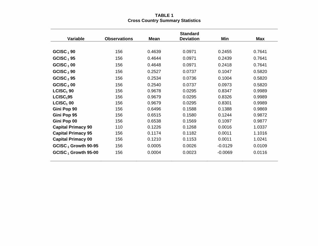
TABLE 1 Cross Country Summary Statistics
Variable Observations Mean Standard Deviation Min Max
GCISC 1 90 156 0.4639 0.0971 0.2455 0.7641 GCISC 1 95 156 0.4644 0.0971 0.2439 0.7641 GCISC 1 00 156 0.4648 0.0971 0.2418 0.7641 GCISC 2 90 156 0.2527 0.0737 0.1047 0.5820 GCISC 2 95 156 0.2534 0.0736 0.1004 0.5820 GCISC 2 00 156 0.2540 0.0737 0.0973 0.5820 LCISC1 90 156 0.9678 0.0295 0.8347 0.9989 LCISC195 156 0.9679 0.0295 0.8326 0.9989 LCISC1 00 156 0.9679 0.0295 0.8301 0.9989 Gini Pop 90 156 0.6496 0.1588 0.1388 0.9869 Gini Pop 95 156 0.6515 0.1580 0.1244 0.9872 Gini Pop 00 156 0.6538 0.1569 0.1097 0.9877 Capital Primacy 90 110 0.1226 0.1268 0.0016 1.0337 Capital Primacy 95 156 0.1174 0.1182 0.0011 1.1016 Capital Primacy 00 156 0.1210 0.1153 0.0011 1.0241 GCISC 1 Growth 90-95 156 0.0005 0.0026 -0.0129 0.0109 GCISC 1 Growth 95-00
156
0.0004
0.0023
-0.0069
0.0116
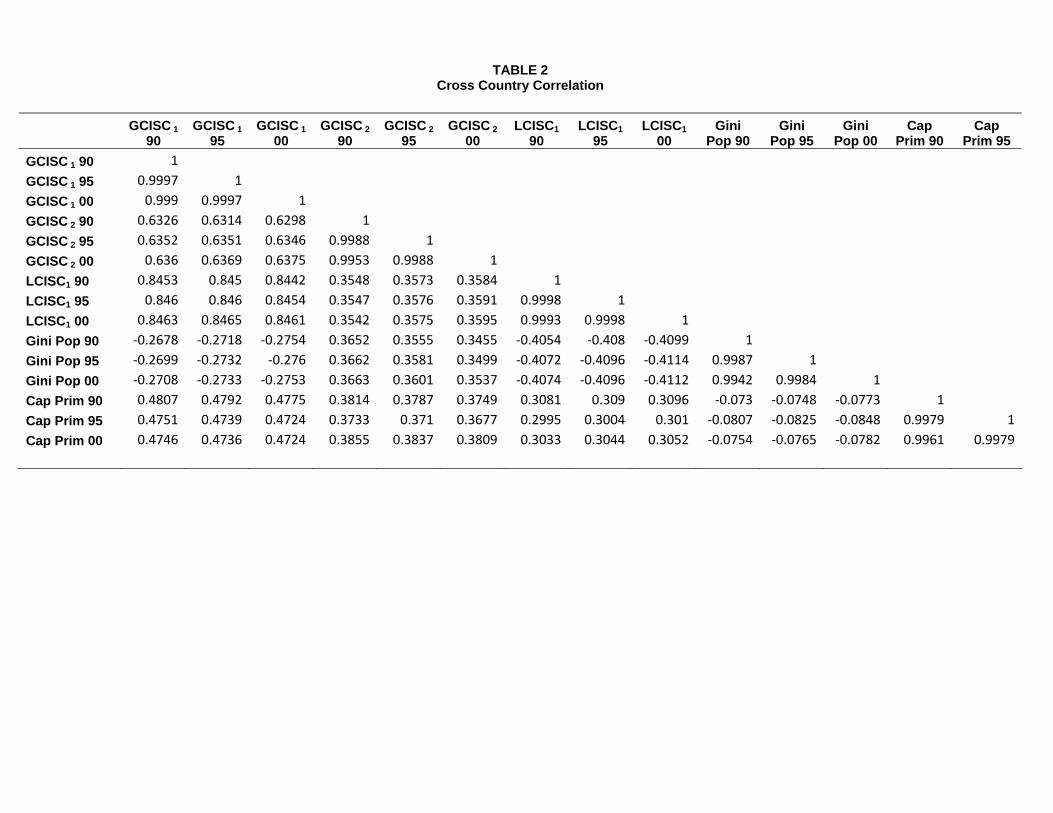
TABLE 2
Cross Country Correlation
GCISC 1
90 GCISC 1
95 GCISC 1
00 GCISC 2
90 GCISC 2
95 GCISC 2
00 LCISC1
90 LCISC1
95 LCISC1
00 Gini
Pop 90 Gini
Pop 95 Gini
Pop 00 Cap
Prim 90 Cap
Prim 95 GCISC 1 90 1 GCISC 1 95 0.9997 1
GCISC 1 00 0.999 0.9997 1 GCISC 2 90 0.6326 0.6314 0.6298 1 GCISC 2 95 0.6352 0.6351 0.6346 0.9988 1 GCISC 2 00 0.636 0.6369 0.6375 0.9953 0.9988 1 LCISC1 90 0.8453 0.845 0.8442 0.3548 0.3573 0.3584 1 LCISC1 95 0.846 0.846 0.8454 0.3547 0.3576 0.3591 0.9998 1 LCISC1 00 0.8463 0.8465 0.8461 0.3542 0.3575 0.3595 0.9993 0.9998 1 Gini Pop 90 ‐0.2678 ‐0.2718 ‐0.2754 0.3652 0.3555 0.3455 ‐0.4054 ‐0.408 ‐0.4099 1 Gini Pop 95 ‐0.2699 ‐0.2732 ‐0.276 0.3662 0.3581 0.3499 ‐0.4072 ‐0.4096 ‐0.4114 0.9987 1 Gini Pop 00 ‐0.2708 ‐0.2733 ‐0.2753 0.3663 0.3601 0.3537 ‐0.4074 ‐0.4096 ‐0.4112 0.9942 0.9984 1 Cap Prim 90 0.4807 0.4792 0.4775 0.3814 0.3787 0.3749 0.3081 0.309 0.3096 ‐0.073 ‐0.0748 ‐0.0773 1
Cap Prim 95 0.4751 0.4739 0.4724 0.3733 0.371 0.3677 0.2995 0.3004 0.301 ‐0.0807 ‐0.0825 ‐0.0848 0.9979 1
Cap Prim 00 0.4746 0.4736 0.4724 0.3855 0.3837 0.3809 0.3033 0.3044 0.3052 ‐0.0754 ‐0.0765 ‐0.0782 0.9961 0.9979
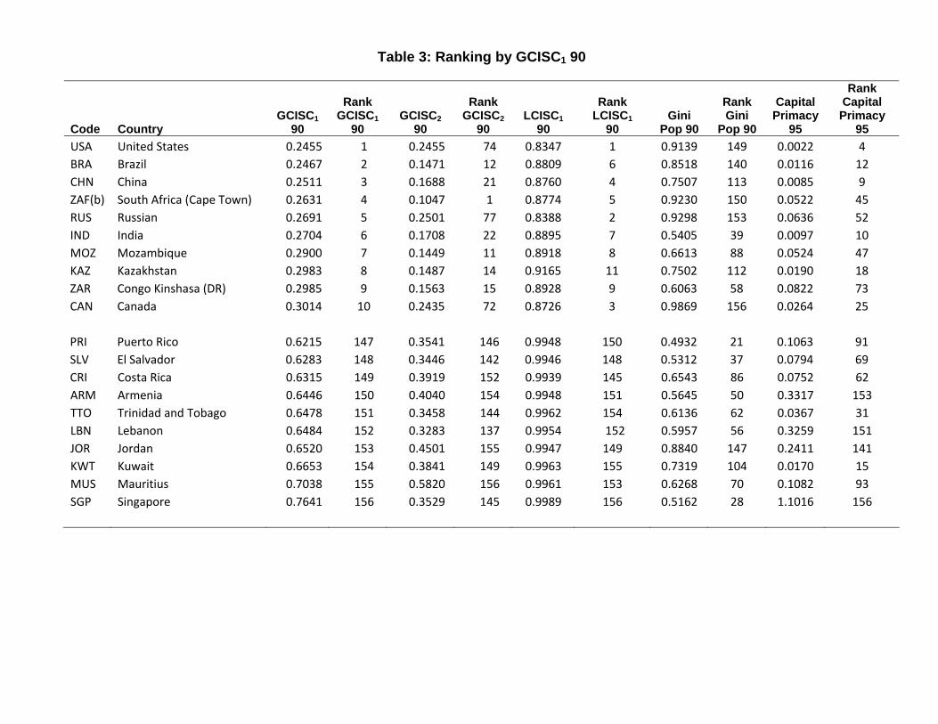
Table 3: Ranking by GCISC1 90
Code Country GCISC1
90
Rank GCISC1
90 GCISC2
90
Rank GCISC2
90 LCISC1
90
Rank LCISC1
90 Gini
Pop 90
Rank Gini
Pop 90
Capital Primacy
95
Rank Capital Primacy
95 USA United States 0.2455 1 0.2455 74 0.8347 1 0.9139 149 0.0022 4 BRA Brazil 0.2467 2 0.1471 12 0.8809 6 0.8518 140 0.0116 12 CHN China 0.2511 3 0.1688 21 0.8760 4 0.7507 113 0.0085 9 ZAF(b) South Africa (Cape Town) 0.2631 4 0.1047 1 0.8774 5 0.9230 150 0.0522 45 RUS Russian 0.2691 5 0.2501 77 0.8388 2 0.9298 153 0.0636 52 IND India 0.2704 6 0.1708 22 0.8895 7 0.5405 39 0.0097 10 MOZ Mozambique 0.2900 7 0.1449 11 0.8918 8 0.6613 88 0.0524 47 KAZ Kazakhstan 0.2983 8 0.1487 14 0.9165 11 0.7502 112 0.0190 18 ZAR Congo Kinshasa (DR) 0.2985 9 0.1563 15 0.8928 9 0.6063 58 0.0822 73 CAN Canada 0.3014 10 0.2435 72 0.8726 3 0.9869 156 0.0264 25
PRI Puerto Rico 0.6215 147 0.3541 146 0.9948 150 0.4932 21 0.1063 91 SLV El Salvador 0.6283 148 0.3446 142 0.9946 148 0.5312 37 0.0794 69 CRI Costa Rica 0.6315 149 0.3919 152 0.9939 145 0.6543 86 0.0752 62 ARM Armenia 0.6446 150 0.4040 154 0.9948 151 0.5645 50 0.3317 153 TTO Trinidad and Tobago 0.6478 151 0.3458 144 0.9962 154 0.6136 62 0.0367 31 LBN Lebanon 0.6484 152 0.3283 137 0.9954 152 0.5957 56 0.3259 151 JOR Jordan 0.6520 153 0.4501 155 0.9947 149 0.8840 147 0.2411 141 KWT Kuwait 0.6653 154 0.3841 149 0.9963 155 0.7319 104 0.0170 15 MUS Mauritius 0.7038 155 0.5820 156 0.9961 153 0.6268 70 0.1082 93 SGP Singapore 0.7641 156 0.3529 145 0.9989 156 0.5162 28 1.1016 156
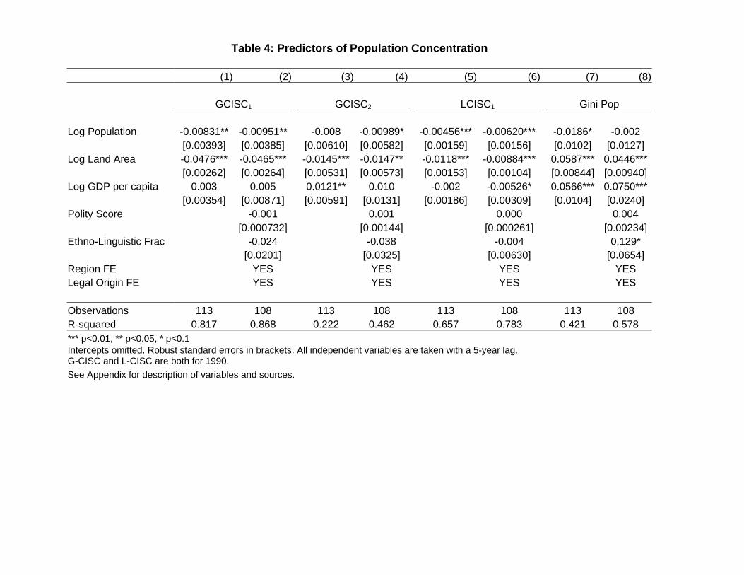
Table 4: Predictors of Population Concentration
(1) (2) (3) (4) (5) (6) (7) (8) GCISC1 GCISC2 LCISC1 Gini Pop Log Population -0.00831** -0.00951** -0.008 -0.00989* -0.00456*** -0.00620*** -0.0186* -0.002 [0.00393] [0.00385] [0.00610] [0.00582] [0.00159] [0.00156] [0.0102] [0.0127] Log Land Area -0.0476*** -0.0465*** -0.0145*** -0.0147** -0.0118*** -0.00884*** 0.0587*** 0.0446*** [0.00262] [0.00264] [0.00531] [0.00573] [0.00153] [0.00104] [0.00844] [0.00940]Log GDP per capita 0.003 0.005 0.0121** 0.010 -0.002 -0.00526* 0.0566*** 0.0750*** [0.00354] [0.00871] [0.00591] [0.0131] [0.00186] [0.00309] [0.0104] [0.0240] Polity Score -0.001 0.001 0.000 0.004 [0.000732] [0.00144] [0.000261] [0.00234]Ethno-Linguistic Frac -0.024 -0.038 -0.004 0.129* [0.0201] [0.0325] [0.00630] [0.0654] Region FE YES YES YES YES Legal Origin FE YES YES YES YES Observations 113 108 113 108 113 108 113 108 R-squared 0.817 0.868 0.222 0.462 0.657 0.783 0.421 0.578 *** p<0.01, ** p<0.05, * p<0.1 Intercepts omitted. Robust standard errors in brackets. All independent variables are taken with a 5-year lag. G-CISC and L-CISC are both for 1990. See Appendix for description of variables and sources.
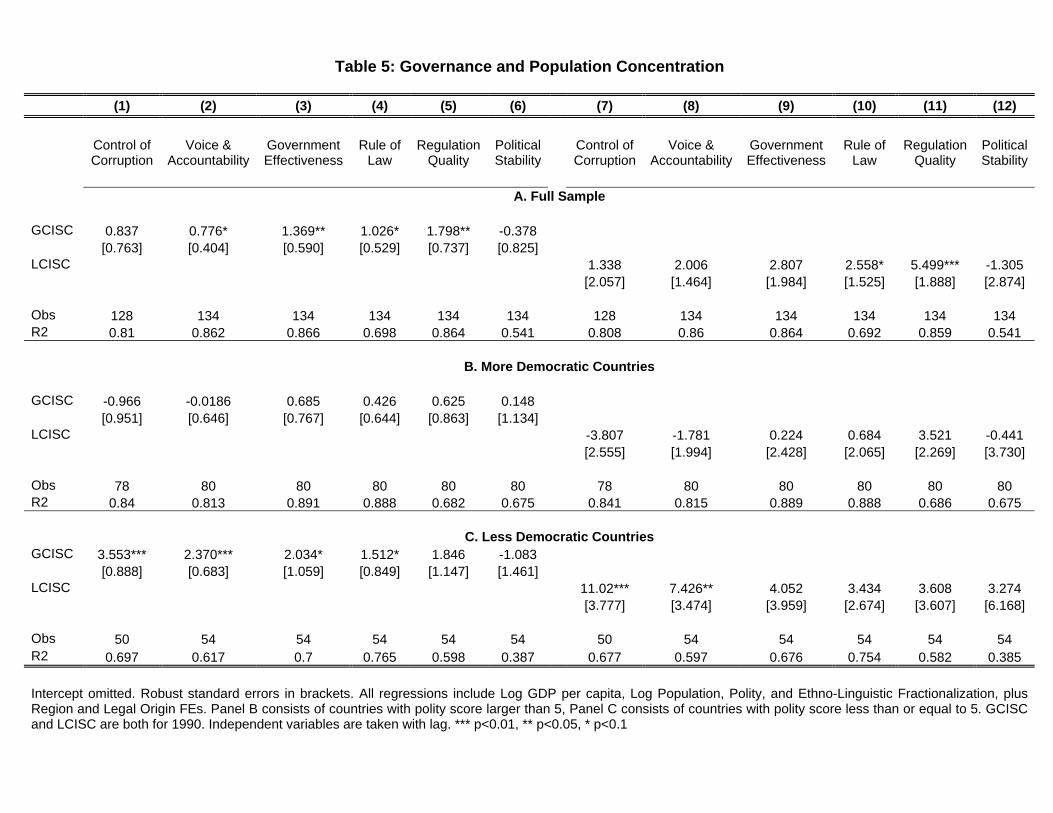
Table 5: Governance and Population Concentration
(1) (2) (3) (4) (5) (6) (7) (8) (9) (10) (11) (12)
Control of Corruption
Voice & Accountability
Government Effectiveness
Rule of Law
Regulation Quality
Political Stability Control of
Corruption Voice &
AccountabilityGovernment Effectiveness
Rule of Law
Regulation Quality
Political Stability
A. Full Sample GCISC 0.837 0.776* 1.369** 1.026* 1.798** -0.378 [0.763] [0.404] [0.590] [0.529] [0.737] [0.825] LCISC 1.338 2.006 2.807 2.558* 5.499*** -1.305 [2.057] [1.464] [1.984] [1.525] [1.888] [2.874] Obs 128 134 134 134 134 134 128 134 134 134 134 134 R2 0.81 0.862 0.866 0.698 0.864 0.541 0.808 0.86 0.864 0.692 0.859 0.541 B. More Democratic Countries GCISC -0.966 -0.0186 0.685 0.426 0.625 0.148 [0.951] [0.646] [0.767] [0.644] [0.863] [1.134] LCISC -3.807 -1.781 0.224 0.684 3.521 -0.441 [2.555] [1.994] [2.428] [2.065] [2.269] [3.730] Obs 78 80 80 80 80 80 78 80 80 80 80 80 R2 0.84 0.813 0.891 0.888 0.682 0.675 0.841 0.815 0.889 0.888 0.686 0.675 C. Less Democratic Countries GCISC 3.553*** 2.370*** 2.034* 1.512* 1.846 -1.083 [0.888] [0.683] [1.059] [0.849] [1.147] [1.461] LCISC 11.02*** 7.426** 4.052 3.434 3.608 3.274 [3.777] [3.474] [3.959] [2.674] [3.607] [6.168] Obs 50 54 54 54 54 54 50 54 54 54 54 54 R2 0.697 0.617 0.7 0.765 0.598 0.387 0.677 0.597 0.676 0.754 0.582 0.385 Intercept omitted. Robust standard errors in brackets. All regressions include Log GDP per capita, Log Population, Polity, and Ethno-Linguistic Fractionalization, plus Region and Legal Origin FEs. Panel B consists of countries with polity score larger than 5, Panel C consists of countries with polity score less than or equal to 5. GCISC and LCISC are both for 1990. Independent variables are taken with lag. *** p<0.01, ** p<0.05, * p<0.1
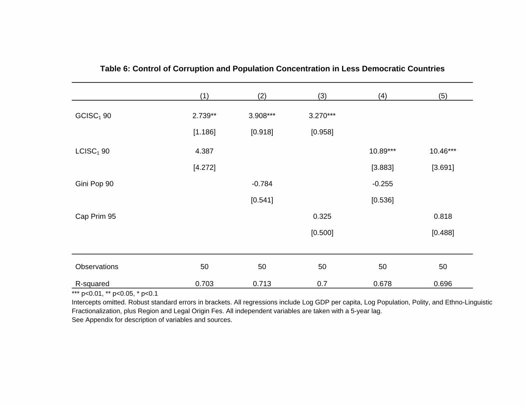
Table 6: Control of Corruption and Population Concentration in Less Democratic Countries
(1) (2) (3) (4) (5)
GCISC1 90 2.739** 3.908*** 3.270***
[1.186] [0.918] [0.958]
LCISC1 90 4.387 10.89*** 10.46***
[4.272] [3.883] [3.691]
Gini Pop 90 -0.784 -0.255
[0.541] [0.536]
Cap Prim 95 0.325 0.818
[0.500] [0.488]
Observations 50 50 50 50 50
R-squared 0.703 0.713 0.7 0.678 0.696 *** p<0.01, ** p<0.05, * p<0.1 Intercepts omitted. Robust standard errors in brackets. All regressions include Log GDP per capita, Log Population, Polity, and Ethno-Linguistic Fractionalization, plus Region and Legal Origin Fes. All independent variables are taken with a 5-year lag. See Appendix for description of variables and sources.
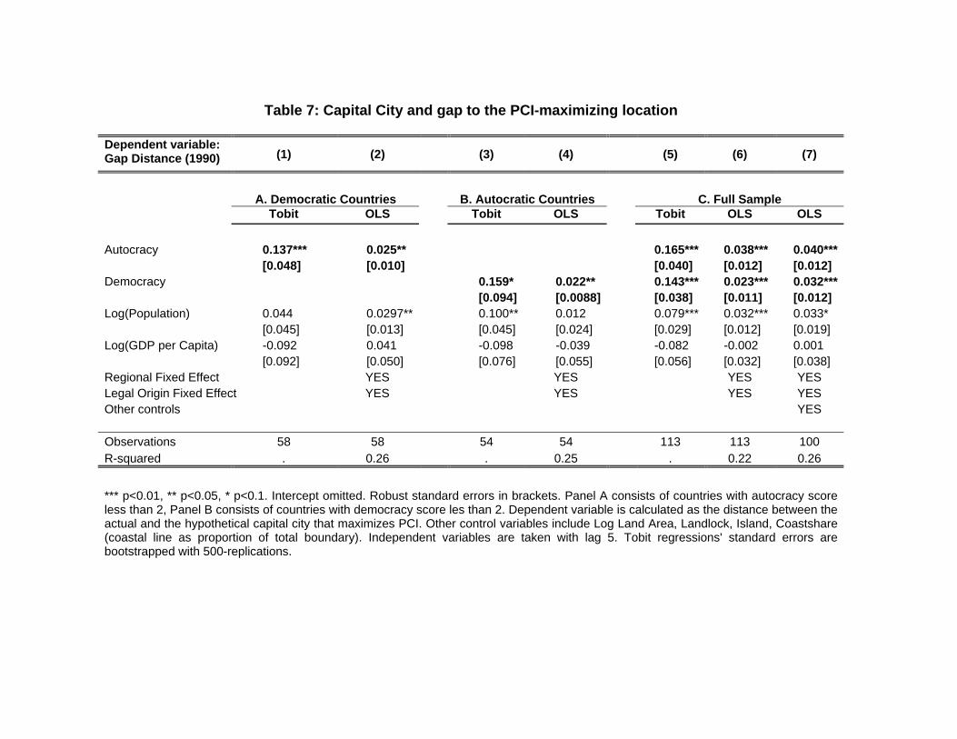
Table 7: Capital City and gap to the PCI-maximizing location Dependent variable: Gap Distance (1990) (1) (2) (3) (4) (5) (6) (7)
A. Democratic Countries B. Autocratic Countries C. Full Sample Tobit OLS Tobit OLS Tobit OLS OLS Autocracy 0.137*** 0.025** 0.165*** 0.038*** 0.040*** [0.048] [0.010] [0.040] [0.012] [0.012] Democracy 0.159* 0.022** 0.143*** 0.023*** 0.032*** [0.094] [0.0088] [0.038] [0.011] [0.012] Log(Population) 0.044 0.0297** 0.100** 0.012 0.079*** 0.032*** 0.033* [0.045] [0.013] [0.045] [0.024] [0.029] [0.012] [0.019] Log(GDP per Capita) -0.092 0.041 -0.098 -0.039 -0.082 -0.002 0.001 [0.092] [0.050] [0.076] [0.055] [0.056] [0.032] [0.038] Regional Fixed Effect YES YES YES YES Legal Origin Fixed Effect YES YES YES YES Other controls YES Observations 58 58 54 54 113 113 100 R-squared . 0.26 . 0.25 . 0.22 0.26
*** p<0.01, ** p<0.05, * p<0.1. Intercept omitted. Robust standard errors in brackets. Panel A consists of countries with autocracy score less than 2, Panel B consists of countries with democracy score les than 2. Dependent variable is calculated as the distance between the actual and the hypothetical capital city that maximizes PCI. Other control variables include Log Land Area, Landlock, Island, Coastshare (coastal line as proportion of total boundary). Independent variables are taken with lag 5. Tobit regressions' standard errors are bootstrapped with 500-replications.
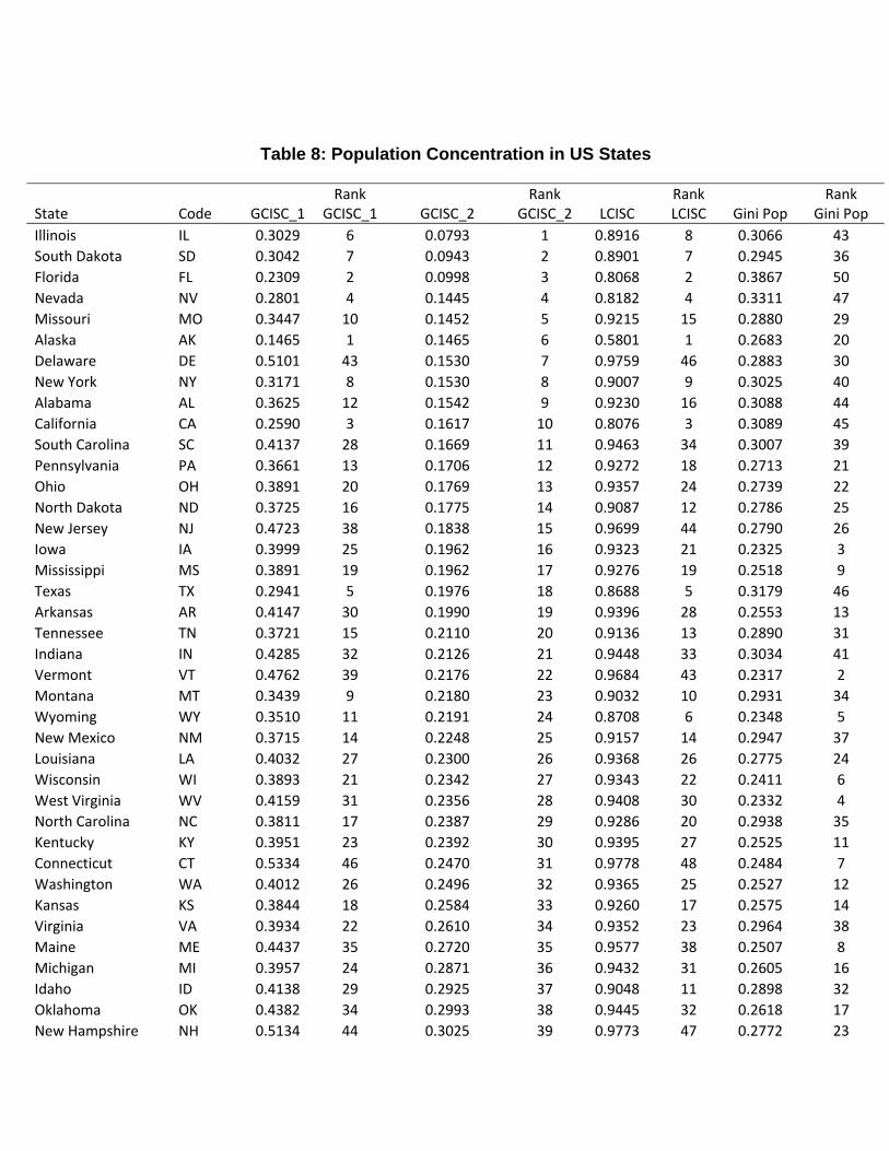
Table 8: Population Concentration in US States
State Code GCISC_1 Rank
GCISC_1 GCISC_2 Rank
GCISC_2 LCISC Rank LCISC Gini Pop
Rank Gini Pop
Illinois IL 0.3029 6 0.0793 1 0.8916 8 0.3066 43 South Dakota SD 0.3042 7 0.0943 2 0.8901 7 0.2945 36 Florida FL 0.2309 2 0.0998 3 0.8068 2 0.3867 50 Nevada NV 0.2801 4 0.1445 4 0.8182 4 0.3311 47 Missouri MO 0.3447 10 0.1452 5 0.9215 15 0.2880 29 Alaska AK 0.1465 1 0.1465 6 0.5801 1 0.2683 20 Delaware DE 0.5101 43 0.1530 7 0.9759 46 0.2883 30 New York NY 0.3171 8 0.1530 8 0.9007 9 0.3025 40 Alabama AL 0.3625 12 0.1542 9 0.9230 16 0.3088 44 California CA 0.2590 3 0.1617 10 0.8076 3 0.3089 45 South Carolina SC 0.4137 28 0.1669 11 0.9463 34 0.3007 39 Pennsylvania PA 0.3661 13 0.1706 12 0.9272 18 0.2713 21 Ohio OH 0.3891 20 0.1769 13 0.9357 24 0.2739 22 North Dakota ND 0.3725 16 0.1775 14 0.9087 12 0.2786 25 New Jersey NJ 0.4723 38 0.1838 15 0.9699 44 0.2790 26 Iowa IA 0.3999 25 0.1962 16 0.9323 21 0.2325 3 Mississippi MS 0.3891 19 0.1962 17 0.9276 19 0.2518 9 Texas TX 0.2941 5 0.1976 18 0.8688 5 0.3179 46 Arkansas AR 0.4147 30 0.1990 19 0.9396 28 0.2553 13 Tennessee TN 0.3721 15 0.2110 20 0.9136 13 0.2890 31 Indiana IN 0.4285 32 0.2126 21 0.9448 33 0.3034 41 Vermont VT 0.4762 39 0.2176 22 0.9684 43 0.2317 2 Montana MT 0.3439 9 0.2180 23 0.9032 10 0.2931 34 Wyoming WY 0.3510 11 0.2191 24 0.8708 6 0.2348 5 New Mexico NM 0.3715 14 0.2248 25 0.9157 14 0.2947 37 Louisiana LA 0.4032 27 0.2300 26 0.9368 26 0.2775 24 Wisconsin WI 0.3893 21 0.2342 27 0.9343 22 0.2411 6 West Virginia WV 0.4159 31 0.2356 28 0.9408 30 0.2332 4 North Carolina NC 0.3811 17 0.2387 29 0.9286 20 0.2938 35 Kentucky KY 0.3951 23 0.2392 30 0.9395 27 0.2525 11 Connecticut CT 0.5334 46 0.2470 31 0.9778 48 0.2484 7 Washington WA 0.4012 26 0.2496 32 0.9365 25 0.2527 12 Kansas KS 0.3844 18 0.2584 33 0.9260 17 0.2575 14 Virginia VA 0.3934 22 0.2610 34 0.9352 23 0.2964 38 Maine ME 0.4437 35 0.2720 35 0.9577 38 0.2507 8 Michigan MI 0.3957 24 0.2871 36 0.9432 31 0.2605 16 Idaho ID 0.4138 29 0.2925 37 0.9048 11 0.2898 32 Oklahoma OK 0.4382 34 0.2993 38 0.9445 32 0.2618 17 New Hampshire NH 0.5134 44 0.3025 39 0.9773 47 0.2772 23
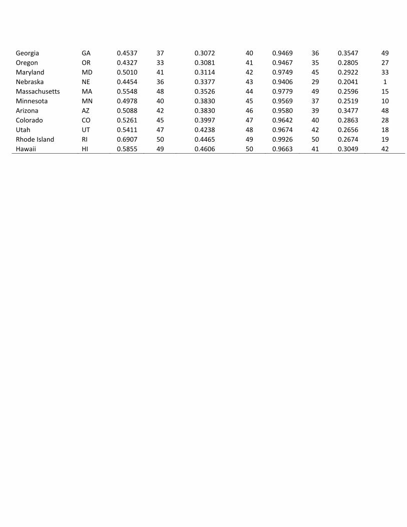
Georgia GA 0.4537 37 0.3072 40 0.9469 36 0.3547 49 Oregon OR 0.4327 33 0.3081 41 0.9467 35 0.2805 27 Maryland MD 0.5010 41 0.3114 42 0.9749 45 0.2922 33 Nebraska NE 0.4454 36 0.3377 43 0.9406 29 0.2041 1 Massachusetts MA 0.5548 48 0.3526 44 0.9779 49 0.2596 15 Minnesota MN 0.4978 40 0.3830 45 0.9569 37 0.2519 10 Arizona AZ 0.5088 42 0.3830 46 0.9580 39 0.3477 48 Colorado CO 0.5261 45 0.3997 47 0.9642 40 0.2863 28 Utah UT 0.5411 47 0.4238 48 0.9674 42 0.2656 18 Rhode Island RI 0.6907 50 0.4465 49 0.9926 50 0.2674 19 Hawaii HI 0.5855 49 0.4606 50 0.9663 41 0.3049 42
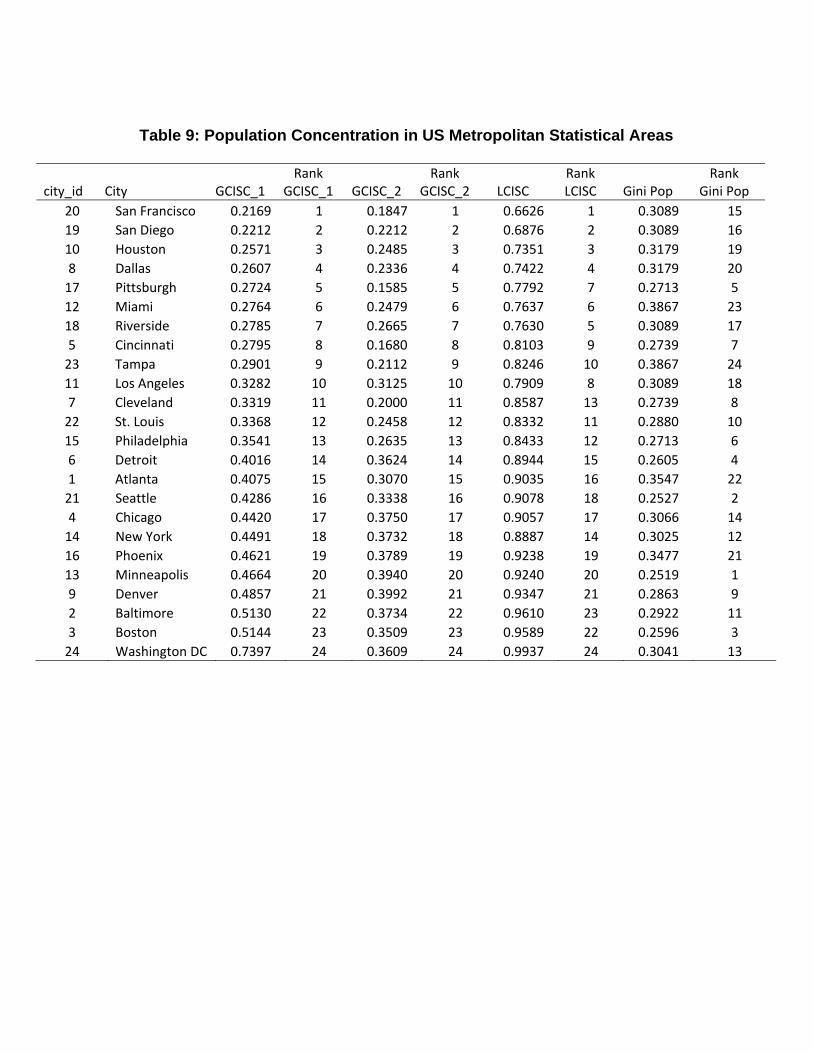
Table 9: Population Concentration in US Metropolitan Statistical Areas
city_id City GCISC_1 Rank
GCISC_1 GCISC_2 Rank
GCISC_2 LCISC Rank LCISC Gini Pop
Rank Gini Pop
20 San Francisco 0.2169 1 0.1847 1 0.6626 1 0.3089 15 19 San Diego 0.2212 2 0.2212 2 0.6876 2 0.3089 16 10 Houston 0.2571 3 0.2485 3 0.7351 3 0.3179 19 8 Dallas 0.2607 4 0.2336 4 0.7422 4 0.3179 20 17 Pittsburgh 0.2724 5 0.1585 5 0.7792 7 0.2713 5 12 Miami 0.2764 6 0.2479 6 0.7637 6 0.3867 23 18 Riverside 0.2785 7 0.2665 7 0.7630 5 0.3089 17 5 Cincinnati 0.2795 8 0.1680 8 0.8103 9 0.2739 7 23 Tampa 0.2901 9 0.2112 9 0.8246 10 0.3867 24 11 Los Angeles 0.3282 10 0.3125 10 0.7909 8 0.3089 18 7 Cleveland 0.3319 11 0.2000 11 0.8587 13 0.2739 8 22 St. Louis 0.3368 12 0.2458 12 0.8332 11 0.2880 10 15 Philadelphia 0.3541 13 0.2635 13 0.8433 12 0.2713 6 6 Detroit 0.4016 14 0.3624 14 0.8944 15 0.2605 4 1 Atlanta 0.4075 15 0.3070 15 0.9035 16 0.3547 22 21 Seattle 0.4286 16 0.3338 16 0.9078 18 0.2527 2 4 Chicago 0.4420 17 0.3750 17 0.9057 17 0.3066 14 14 New York 0.4491 18 0.3732 18 0.8887 14 0.3025 12 16 Phoenix 0.4621 19 0.3789 19 0.9238 19 0.3477 21 13 Minneapolis 0.4664 20 0.3940 20 0.9240 20 0.2519 1 9 Denver 0.4857 21 0.3992 21 0.9347 21 0.2863 9 2 Baltimore 0.5130 22 0.3734 22 0.9610 23 0.2922 11 3 Boston 0.5144 23 0.3509 23 0.9589 22 0.2596 3 24 Washington DC 0.7397 24 0.3609 24 0.9937 24 0.3041 13