Embed Size (px)
Citation preview
Faculty of Mechanical Engineering and Marine Technology
Chair of Modelling and Simulation
Ship dynamics in waves(Ship Theory II)
Prof. Dr.-Ing. habil. Nikolai Kornev
Rostock2012

2
Contents
1 Small ship motion in regular sea waves 11
1.1 Coupling of different ship oscillations . . . . . . . . . . . . . . 11
1.2 Classification of forces . . . . . . . . . . . . . . . . . . . . . . 12
1.3 Radiation force components . . . . . . . . . . . . . . . . . . . 17
1.3.1 Hydrodynamic damping . . . . . . . . . . . . . . . . . 18
1.3.2 Added mass component . . . . . . . . . . . . . . . . . 21
1.4 Hydrostatic component . . . . . . . . . . . . . . . . . . . . . . 24
1.5 Wave exciting force . . . . . . . . . . . . . . . . . . . . . . . . 24
1.6 Motion equations . . . . . . . . . . . . . . . . . . . . . . . . . 25
1.7 Haskind’s relation . . . . . . . . . . . . . . . . . . . . . . . . . 25
1.8 Exercises . . . . . . . . . . . . . . . . . . . . . . . . . . . . . . 27
2 Free oscillations with small amplitudes 31
2.1 Theory . . . . . . . . . . . . . . . . . . . . . . . . . . . . . . . 31
2.2 Exercise . . . . . . . . . . . . . . . . . . . . . . . . . . . . . . 34
3 Ship oscillations in small transverse waves (beam see) 37
3.1 Hydrostatic forces and moments . . . . . . . . . . . . . . . . . 38
3.2 Hydrodynamic Krylov - Froude force . . . . . . . . . . . . . . 40
3.3 Full Krylov - Froude force and moment . . . . . . . . . . . . . 42
3.4 Force and moment acting on the ship frame in accelerated flow 42
3.5 Full wave induced force and moment . . . . . . . . . . . . . . 43
3.6 Equations of ship heave and roll oscillations . . . . . . . . . . 43
3.7 Analysis of the formula (3.27) . . . . . . . . . . . . . . . . . . 46
3.8 Sway ship oscillations in beam sea . . . . . . . . . . . . . . . . 49
3.9 Ship oscillations at finite beam to wave length ratio and draughtto length ratio . . . . . . . . . . . . . . . . . . . . . . . . . . . 50
3.10 Effect of ship speed on rolling . . . . . . . . . . . . . . . . . . 53
3
4 Ship oscillations in small head waves 574.1 Exciting forces and ship oscillations . . . . . . . . . . . . . . . 574.2 Estimations of slamming and deck flooding . . . . . . . . . . . 61
5 Seasickness caused by ship oscillations 65
6 Ship oscillations in irregular waves 696.1 Representation of irregular waves . . . . . . . . . . . . . . . . 69
6.1.1 Wave ordinates as stochastic quantities . . . . . . . . . 706.1.2 Wave spectra . . . . . . . . . . . . . . . . . . . . . . . 73
6.2 Calculation of ship oscillations in irregular waves . . . . . . . 76
7 Experimental methods in ship seakeeping 797.1 Experiments with models . . . . . . . . . . . . . . . . . . . . . 79
7.1.1 Similarity criteria . . . . . . . . . . . . . . . . . . . . . 797.1.2 Geometric parameters . . . . . . . . . . . . . . . . . . 807.1.3 Free oscillation tests . . . . . . . . . . . . . . . . . . . 837.1.4 Forced oscillation at calm water conditions . . . . . . . 857.1.5 Seakeeping tests . . . . . . . . . . . . . . . . . . . . . . 86
7.2 Seakeeping tests with large scale ships . . . . . . . . . . . . . 87
8 Ship oscillation damping (stabilisation) 898.1 Introduction . . . . . . . . . . . . . . . . . . . . . . . . . . . . 898.2 Damping of roll oscillations . . . . . . . . . . . . . . . . . . . 90
8.2.1 Passive systems . . . . . . . . . . . . . . . . . . . . . . 908.2.2 Theory . . . . . . . . . . . . . . . . . . . . . . . . . . . 938.2.3 Active stabilizing system . . . . . . . . . . . . . . . . . 968.2.4 Bilge keel . . . . . . . . . . . . . . . . . . . . . . . . . 968.2.5 Rudders . . . . . . . . . . . . . . . . . . . . . . . . . . 98
8.3 Stabilizing systems for pitch oscillations . . . . . . . . . . . . 99
9 Parametric oscillations 101
10 Potential methods for calculation of forces acting on the os-cillating ships 10510.1 Strip theory . . . . . . . . . . . . . . . . . . . . . . . . . . . . 10510.2 Principles of Rankine source method for calculation of sea-
keeping . . . . . . . . . . . . . . . . . . . . . . . . . . . . . . . 10910.2.1 Frequency domain simulations . . . . . . . . . . . . . . 10910.2.2 Time domain simulation (TDS) . . . . . . . . . . . . . 115
4
List of Tables
2.1 Frequencies and periods of different oscillation types . . . . . . 332.2 Referred damping factors for different oscillation types . . . . 34
8.1 Comparison of different stabilizing systems (taken from [1]) . . 998.2 ... . . . . . . . . . . . . . . . . . . . . . . . . . . . . . . . . . . 100
5

6
List of Figures
1.1 Ship motion with 6 degree of freedom (from [2]) . . . . . . . . 121.2 Displacement of the center of effort due to change of the ship
draught (from [3]) . . . . . . . . . . . . . . . . . . . . . . . . . 131.3 Illustration to derivation of damping coefficient . . . . . . . . 191.4 Added mass and damping coefficient of the semi circle frame
at heave oscillations. Here A is the frame area. . . . . . . . . . 201.5 Added mass and damping coefficient of the box frame at heave
oscillations. Here A is the frame area. . . . . . . . . . . . . . . 211.6 Added mass and damping coefficient of the semi circle frame
at sway oscillations. Here A is the frame area. . . . . . . . . . 211.7 Added mass and damping coefficient of the box frame at sway
oscillations. Here A is the frame area. . . . . . . . . . . . . . . 211.8 Added mass and damping coefficient of the box frame at roll
(heel) oscillations. Here A is the frame area. . . . . . . . . . . 221.9 Mirroring for the case ω → 0 . . . . . . . . . . . . . . . . . . . 231.10 Mirroring for the case ω →∞ . . . . . . . . . . . . . . . . . . 231.11 Bild aus Buch von Newman . . . . . . . . . . . . . . . . . . . 29
3.1 . . . . . . . . . . . . . . . . . . . . . . . . . . . . . . . . . . . 383.2 Illustration of hydrostatic force . . . . . . . . . . . . . . . . . 393.3 Illustration of hydrostatic moment . . . . . . . . . . . . . . . . 393.4 Ship as linear system . . . . . . . . . . . . . . . . . . . . . . . 463.5 Response function versus referred frequency . . . . . . . . . . 473.6 Phase displacement versus referred frequency . . . . . . . . . . 483.7 Ship oscillations in resonance case . . . . . . . . . . . . . . . . 483.8 Oscillation of a raft with a big metacentric height . . . . . . . 483.9 Illustration of the frame in beam waves . . . . . . . . . . . . . 493.10 . . . . . . . . . . . . . . . . . . . . . . . . . . . . . . . . . . . 513.11 Reduction coefficient of the heave oscillations . . . . . . . . . 533.12 Sea classification . . . . . . . . . . . . . . . . . . . . . . . . . 54
4.1 Illustration of the ship in head waves . . . . . . . . . . . . . . 57
7
4.2 Position of ship at different time instants in a head wave . . . 614.3 Curves y = ±zmax and y = z(x) . . . . . . . . . . . . . . . . . 624.4 Sample for a real ship . . . . . . . . . . . . . . . . . . . . . . . 63
5.1 Influence of the vertical acceleration on the seasickness de-pending on the oscillation period . . . . . . . . . . . . . . . . 65
5.2 Influence of the vertical acceleration on the seasickness de-pending on the oscillation period . . . . . . . . . . . . . . . . 66
5.3 Number of passengers suffering from seasickness on a cruiseliners depending on vertical accelerations . . . . . . . . . . . . 67
5.4 Adaption to seasickness . . . . . . . . . . . . . . . . . . . . . . 67
6.1 Irregular seawaves, 1- two dimensional, 2- three dimensional.(Fig. from [4]) . . . . . . . . . . . . . . . . . . . . . . . . . . . 69
6.2 Profile of an irregular wave. (Fig. from [4]) . . . . . . . . . . . 706.3 Representation of irregular wave through the superposition of
regular waves. (Fig. from [4]) . . . . . . . . . . . . . . . . . . 716.4 p.d.f. of the wave ordinate . . . . . . . . . . . . . . . . . . . . 726.5 . . . . . . . . . . . . . . . . . . . . . . . . . . . . . . . . . . . 75
7.1 Determination of the inertia moment Izzm . . . . . . . . . . . 817.2 α is the angle between rod and the vertical . . . . . . . . . . . 817.3 Determination of Ixxm and zg . . . . . . . . . . . . . . . . . . 837.4 Heel test . . . . . . . . . . . . . . . . . . . . . . . . . . . . . . 847.5 Method of forced rolling . . . . . . . . . . . . . . . . . . . . . 857.6 Seakeeping test at MARIN ([5]) . . . . . . . . . . . . . . . . . 877.7 Scetch of the MARIN Seakeeping basin ([5]) . . . . . . . . . . 877.8 Wave generator of MARIN Seakeeping basin ([5]) . . . . . . . 877.9 Method of wave detection . . . . . . . . . . . . . . . . . . . . 887.10 Ship motion during large scale tests . . . . . . . . . . . . . . . 88
8.1 Schematical representation of the Frahm tank of the first type. 908.2 U-tube passive roll stabilization system manufactured by Hoppe
Marine (http://www.hoppe-marine.com/). Orange tube theare air channel. Picture is taken from [1]. . . . . . . . . . . . . 91
8.3 Response function verus referred frequency without (solid line)and with (dashed line) stabilization system. . . . . . . . . . . 92
8.4 U-tube stabilization system of Frahm of the second type . . . 928.5 Free surface Type passive Roll stabilization systems of Flume . 938.6 Free surface Type passive Roll stabilization systems of Flume . 938.7 Offshore Support Vessel [1] . . . . . . . . . . . . . . . . . . . . 938.8 Research Ship [1] . . . . . . . . . . . . . . . . . . . . . . . . . 94
8
8.9 Offshore Patrol Vessel [1] . . . . . . . . . . . . . . . . . . . . . 948.10 Passenger Ship [1] . . . . . . . . . . . . . . . . . . . . . . . . . 948.11 Reduction of the roll amplitude using the Flume tank designed
by Hoppe Marine (taken from [1]). . . . . . . . . . . . . . . . 958.12 Active stabilizing system . . . . . . . . . . . . . . . . . . . . . 978.13 Bilge keel [1] . . . . . . . . . . . . . . . . . . . . . . . . . . . . 978.14 Main parameters of bilge keels. . . . . . . . . . . . . . . . . . 988.15 Schematic representation of active fins. . . . . . . . . . . . . . 998.16 Active rudder roll. . . . . . . . . . . . . . . . . . . . . . . . . 998.17 Schematic representation of the pitch stabilizing system . . . . 1008.18 Reduction of pitch and heave oscillations using the stabilizing
system. . . . . . . . . . . . . . . . . . . . . . . . . . . . . . . . 100
9.1 Ship oscillations during parametric resonance . . . . . . . . . . 1039.2 Conditions for parametric resonance appearance . . . . . . . . 103
10.1 Assumption of the strip theory [1]. . . . . . . . . . . . . . . . 106
9

10
Chapter 1
Small ship motion in regularsea waves
1.1 Coupling of different ship oscillations
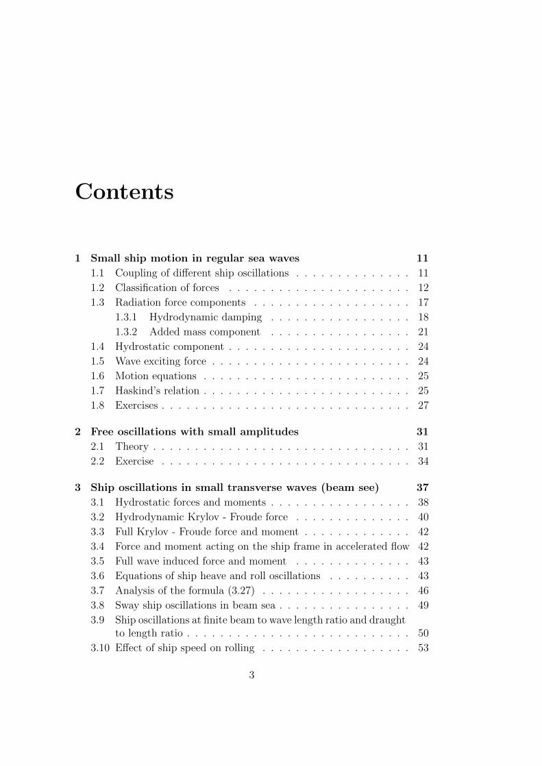
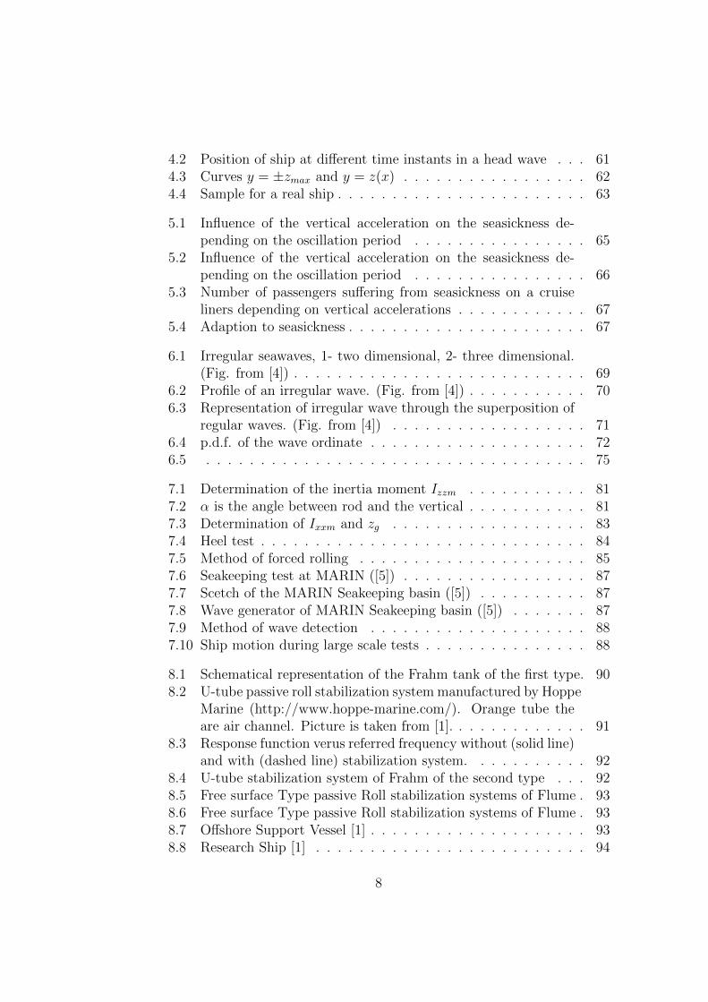
The ship has generally six degrees of freedom which are called as surge ζ,sway η, heave ζ, heel (or roll) ϕ, yaw ϑ and pitch ψ (see Fig.1.1) for expla-nation of each oscillation motion). In this chapter we consider first the caseof the ship with zero forward speed. Generally, different ship oscillations arestrongly coupled. There are three sorts of coupling:
• hydrostatic coupling
• hydrodynamic coupling
• gyroscopics coupling
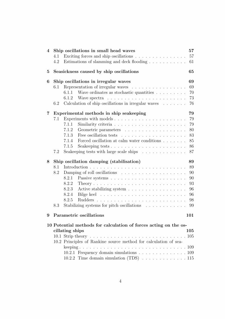
The hydrostatic coupling is illustrated in Fig.1.2. If the ship draught ischanged, the center of effort of vertical hydrostatic (floating) force is mov-ing usually towards the ship stern because the frames in the stern are morefull than those in the bow region. The displacement of the center of efforttowards the stern causes the negative pitch angle. Therefore, the heave os-cillations cause the pitch oscillations and vice versa. With the other words,the heave and pitch oscillations are coupled.
Hydrodynamic coupling can be illustrated when the ship is moving with ac-celeration in transverse direction (sway motion). Since the ship is asymmetricwith respect to the midships, such a motion is conducted with appearance
11
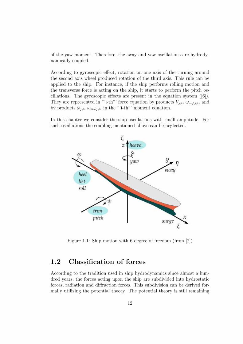
of the yaw moment. Therefore, the sway and yaw oscillations are hydrody-namically coupled.
According to gyroscopic effect, rotation on one axis of the turning aroundthe second axis wheel produced rotation of the third axis. This rule can beapplied to the ship. For instance, if the ship performs rolling motion andthe transverse force is acting on the ship, it starts to perform the pitch os-cillations. The gyroscopic effects are present in the equation system ([6]).They are represented in ”’i-th”’ force equation by products Vj 6=i ωm6=j 6=i andby products ωj 6=i ωm 6=j 6=i in the ”’i-th”’ moment equation.
In this chapter we consider the ship oscillations with small amplitude. Forsuch oscillations the coupling mentioned above can be neglected.
Figure 1.1: Ship motion with 6 degree of freedom (from [2])
1.2 Classification of forces
According to the tradition used in ship hydrodynamics since almost a hun-dred years, the forces acting upon the ship are subdivided into hydrostaticforces, radiation and diffraction forces. This subdivision can be derived for-mally utilizing the potential theory. The potential theory is still remaining
12
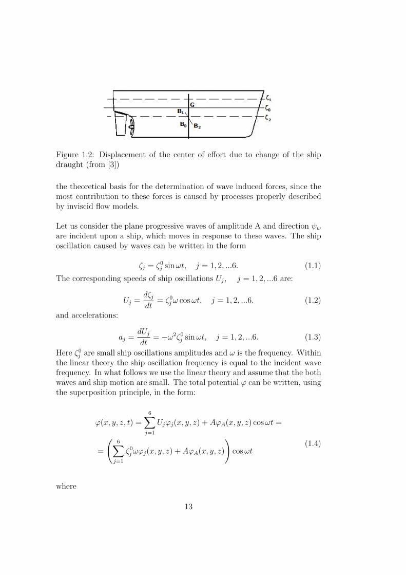
Figure 1.2: Displacement of the center of effort due to change of the shipdraught (from [3])
the theoretical basis for the determination of wave induced forces, since themost contribution to these forces is caused by processes properly describedby inviscid flow models.
Let us consider the plane progressive waves of amplitude A and direction ψware incident upon a ship, which moves in response to these waves. The shiposcillation caused by waves can be written in the form
ζj = ζ0j sinωt, j = 1, 2, ...6. (1.1)
The corresponding speeds of ship oscillations Uj, j = 1, 2, ...6 are:
Uj =dζjdt
= ζ0j ω cosωt, j = 1, 2, ...6. (1.2)
and accelerations:
aj =dUjdt
= −ω2ζ0j sinωt, j = 1, 2, ...6. (1.3)
Here ζ0j are small ship oscillations amplitudes and ω is the frequency. Within
the linear theory the ship oscillation frequency is equal to the incident wavefrequency. In what follows we use the linear theory and assume that the bothwaves and ship motion are small. The total potential ϕ can be written, usingthe superposition principle, in the form:
ϕ(x, y, z, t) =6∑j=1
Ujϕj(x, y, z) + AϕA(x, y, z) cosωt =
=
(6∑j=1
ζ0j ωϕj(x, y, z) + AϕA(x, y, z)
)cosωt
(1.4)
where
13
• ϕj(x, y, z) is the velocity potential of the ship oscillation in j-th motionwith the unit amplitude ζ0
j = 1 in the absence of incident waves,
• ϕA(x, y, z) is the potential taking the incident waves and their interac-tion with the ship into account.
R
The first potentials ϕj(x, y, z) describes the radiation problem , whereasthe second one the wave diffraction problem . The potentials ϕj(x, y, z)and ϕA are independent only in the framework of the linear theory assumingthe waves and ship motions are small. Within this theory ϕA is calculatedfor the ship fixed in position.
The potentials must satisfy the Laplace equation ∆ϕj = 0, ∆ϕA = 0 andappropriate boundary conditions. The boundary conditions to be imposedon the ship surface are the no penetration conditions (see also formulae 3.18in the Chapter 3 [7]):
• for radiation potentials
∂ϕ1
∂n= cos(n, x);
∂ϕ2
∂n= cos(n, y);
∂ϕ3
∂n= cos(n, z);
∂ϕ4
∂n= (y cos(n, z)− z cos(n, y));
∂ϕ5
∂n= (z cos(n, x)− x cos(n, z));
∂ϕ6
∂n= (x cos(n, y)− y cos(n, x)).
(1.5)
• for wave diffraction potentials
∂ϕA∂n
= 0 (1.6)
where n is the normal vector to the ship surface, directed into the body,(x, y, z) are the coordinates of a point on the ship surface. The r.h.s. of theconditions (1.5) is the normal components of the ship local velocities causedby particular oscillating motions.
The diffraction potential ϕA is decomposed in two parts
ϕA = ϕ∞ + ϕp (1.7)
14
which ϕ∞ is the potential of incident waves not perturbed by the ship pres-ence and ϕp is the perturbation potential describing the interaction betweenthe incident waves and the ship. The potential of regular waves ϕ∞ is known(see Chapter 6 in [7]). The boundary condition for ϕp on the ship surface is
∂ϕp∂n
= −∂ϕ∞∂n
(1.8)
Away from the ship the radiation potentials ϕj and the diffraction perturba-tion potential ϕp decay, i.e. ϕp −−−→
r→∞0, ϕj −−−→
r→∞0.
On the free surface the linearized mixed boundary condition (see formula (6.17)in [7]) reads
∂2ϕ
∂t2+ g
∂ϕ
∂z= 0 on z = 0. (1.9)
Substituting (1.4) in (1.9) yields for ϕj(x, y, z) and ϕA(x, y, z):
−ω2
gϕj +
∂ϕj∂z
= 0 on z = 0.
−ω2
gϕA +
∂ϕA∂z
= 0 on z = 0.
(1.10)
It is obvious from (1.10) that ϕj(x, y, z) and ϕA(x, y, z) depend on ω. L
Additionally in the wave theory the radiation condition is imposed statingthat the waves on the free surface caused by the potentials are radiated awayfrom the ship. The potentials introduced above can be found using panelmethods.
The force and the moment on the ship are determined by integrating thepressure over the wetted ship surface. The pressure can be found from theBernoulli equation written in the general form:
p+ρu2
2+ ρgz + ρ
∂ϕ
∂t= C(t) (1.11)
Here the potential is the potential of the perturbed motion. The constant C(t)which is the same for the whole flow domain is calculated from the conditionthat the pressure on the free surface far from the ship is constant and equalto the atmospheric pressure:
pa = C(t) (1.12)
15
Substituting (1.12) in (1.11) gives:
p− pa = −ρu2
2− ρgz − ρ∂ϕ
∂t(1.12a)
Remembering that the ship speed is zero and perturbation velocities as wellas the velocities caused by incident waves are small we neglect the first termin (1.12a):
p− pa = −ρ(∂ϕ
∂t+ gz
)(1.13)
Together with (1.4) it gives
p− pa = ρ
(6∑j=1
ζ0j ωϕj(x, y, z) + AϕA(x, y, z)
)ω sinωt− ρgz (1.14)
The forces and the moment are then calculated by integration of p− pa overthe wetted ship area
~F =
∫S
(p− pa)~ndS, ~M =
∫S
(p− pa)(~r × ~n)dS. (1.15)
The normal vector direction in (1.15) is into the body. The vertical ordi-nate z of any point on the wetted area can be represented as the differencebetween the submergence under unperturbed free surface ζ and free surfaceelevation ζ0. Substituting (1.14) in (1.15) one obtains
~F = −ρg∫S
~nζdS + ρg
∫S
~nζ0dS
+ ρ6∑j=1
ζ0j ω
2 sinωt
∫S
~nϕjdS+
+ ρ(Aω sinωt)
∫S
~n(ϕ∞ + ϕp)dS
(1.16)
Four integrals in (1.16) represent four different contributions to the totalforce:
16
• the hydrostatic component (the first term) acting on the ship oscillatingon the unperturbed free surface (in calm water),
• the hydrostatic component arising due to waves (the second term),
• the damping and the added mass component (the third term) and
• the hydrodynamic wave exciting force (the fourth term).
The moment is expressed through similar components.
The third term describes the force acting on the ship oscillating in calm water.The last term arises due to incident waves acting on the ship. Within the Llinear theory keeping only the terms proportional to the amplitude A andneglecting small terms of higher orders proportional to ∼ An, n > 1 one canshow that the integration in the last term can be done over the wetted areacorresponding to the equilibrium state. Thus, the last term describes theforce induced by waves on the ship at rest. L
1.3 Radiation force components
Let us consider the second term of the force
~F2 = ρ6∑j=1
ζ0j ω
2 sinωt
∫S
~nϕjdS (1.17)
Each component of this force is expressed as
F2i = ρ
6∑j=1
ζ0j ω
2 sinωt
∫S
niϕjdS = −6∑j=1
cjidUjdt
(1.18)
As shown by Haskind [17], the hydrodynamic coefficient cji is represented asthe sum of two coefficients:
cji = µji −1
ωλji
The term − 1ωλji has been introduced to take the fact into account that the
force due to influence of the free surface depends not only on ω2 but alsoon ω. The force is then
17
F2i = −6∑j=1
(µji −
1
ωλji
)dUjdt
= −6∑j=1
µjiaj −6∑j=1
λjiUj
(ts = t− π
2ω
)(1.19)
As seen from (1.19) the first component of the force is proportional to theacceleration aj whereas the second one is proportional to the velocity Uj.The first component is called the added mass component, whereas the sec-ond one- the damping component.
Using the Green’s theorem, Haskind derived the following symmetry condi-tions for the case zero forward speed:
cji = cij ⇒
{µji = µij
λji = λij
1.3.1 Hydrodynamic damping
There are two reasons of the hydrodynamic damping of the ship oscillationson the free surface. First reason is the viscous damping which is proportional
to the square of the ship velocity ∼ CDjρU2
j
2S. Within the linear theory this
term proportional to the amplitude (ζ0j )2 is neglected. The main contribution
to the damping is done by the damping caused by radiated waves. Whenoscillating on the free surface the ship generates waves which have the me-chanic potential and kinetic energy. This wave energy is extracted from thekinetic energy of the ship. Ship transfers its energy to waves which carry itaway from the ship. With the time the whole kinetic energy is radiated awayand the ship oscillations decay.
Similarly to the added mass one can introduce the damping coefficients. Thefull mechanic energy in the progressive wave with the amplitude A is (seechapter 6.4 in [7])
E =1
2ρgA2 (1.20)
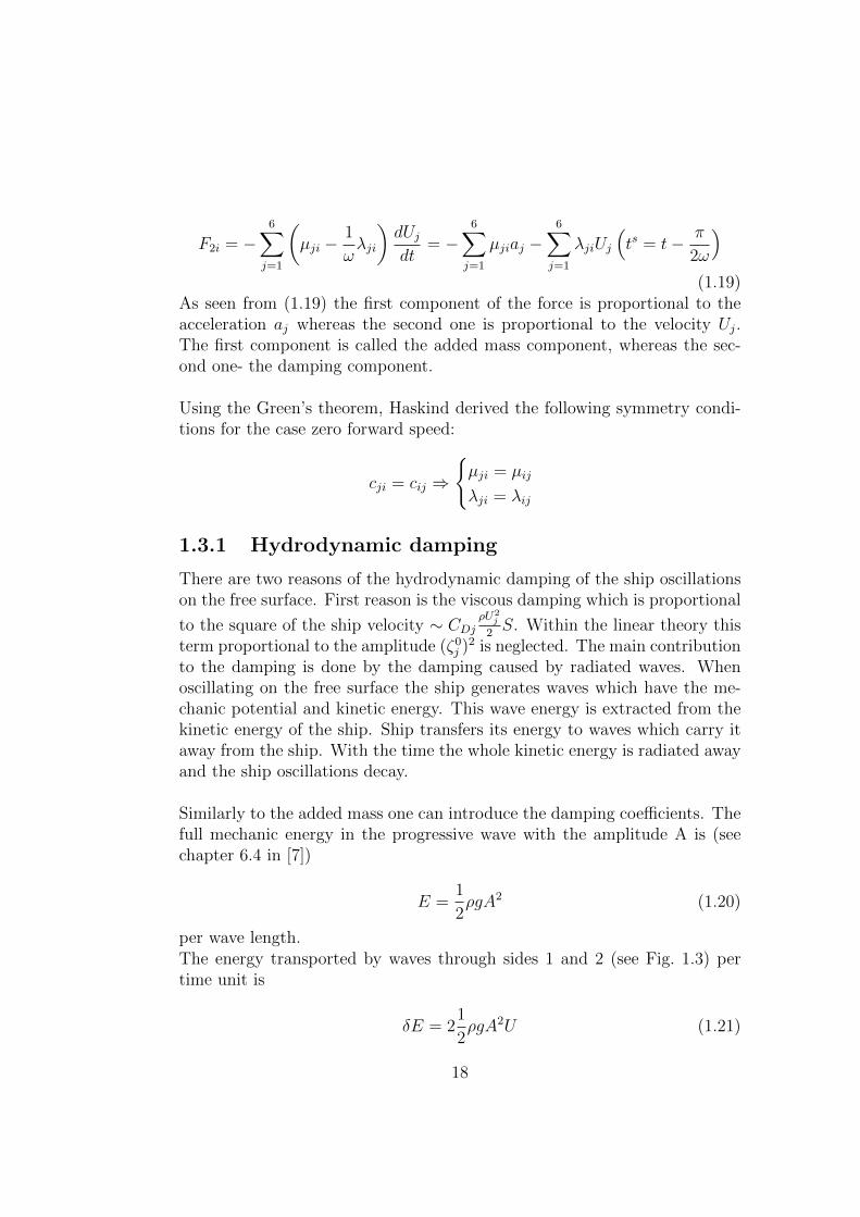
per wave length.The energy transported by waves through sides 1 and 2 (see Fig. 1.3) pertime unit is
δE = 21
2ρgA2U (1.21)
18
Figure 1.3: Illustration to derivation of damping coefficient
where U is the wave group velocity. The damping coefficient is defined as
δE = λijU2j (1.22)
where λij is the coefficient of damping in i-th direction when the ship oscil-
lates in j-th motion. U2j is the time averaged square of the ship oscillations
speed. Obviously, U2j =
(ωζ0j )2
2and
δE = λij
(ωζ0
j
)2
2(1.23)
The group velocity (see formulae (6.39) and (6.40) in [7]):
U =c
2=
1
2
√g
k=
g
2ω(1.24)
since kg = ω2 (see formula (6.21) in [7]). Equating (1.21) and (1.23) oneobtains with account for (1.24)
ρgA2U = λij
(ωζ0
j
)2
2⇓
ρgA2 g
2ω= λij
(ωζ0
j
)2
2⇒ λij =
ρg2
ω3
(A
ζ0j
)2
(1.25)
19
The damping coefficient λij depends on the square of the ratio of the waveamplitude to the ship oscillation amplitude causing the wave.
The damping coefficient of slender body can be found by integration of damp-ing coefficients of ship frames along the ship length
B22 =
L/2∫−L/2
λ22dx, B33 =
L/2∫−L/2
λ33dx, B44 =
L/2∫−L/2
λ44dx,
B55 =
L/2∫−L/2
x2λ33dx, B66 =
L/2∫−L/2
x2λ22dx
(1.26)
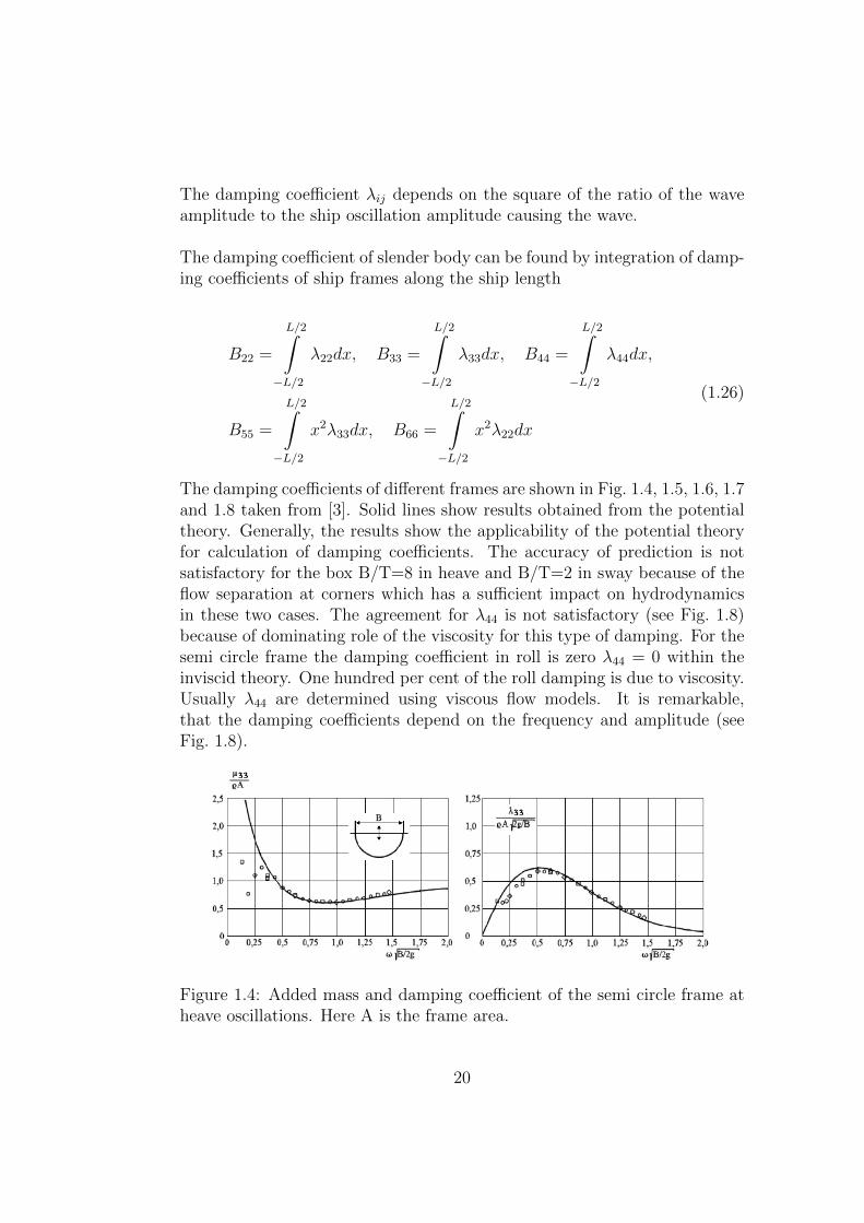
The damping coefficients of different frames are shown in Fig. 1.4, 1.5, 1.6, 1.7and 1.8 taken from [3]. Solid lines show results obtained from the potentialtheory. Generally, the results show the applicability of the potential theoryfor calculation of damping coefficients. The accuracy of prediction is notsatisfactory for the box B/T=8 in heave and B/T=2 in sway because of theflow separation at corners which has a sufficient impact on hydrodynamicsin these two cases. The agreement for λ44 is not satisfactory (see Fig. 1.8)because of dominating role of the viscosity for this type of damping. For thesemi circle frame the damping coefficient in roll is zero λ44 = 0 within theinviscid theory. One hundred per cent of the roll damping is due to viscosity.Usually λ44 are determined using viscous flow models. It is remarkable,that the damping coefficients depend on the frequency and amplitude (seeFig. 1.8).
Figure 1.4: Added mass and damping coefficient of the semi circle frame atheave oscillations. Here A is the frame area.
20
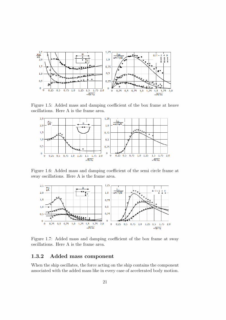
Figure 1.5: Added mass and damping coefficient of the box frame at heaveoscillations. Here A is the frame area.
Figure 1.6: Added mass and damping coefficient of the semi circle frame atsway oscillations. Here A is the frame area.
Figure 1.7: Added mass and damping coefficient of the box frame at swayoscillations. Here A is the frame area.
1.3.2 Added mass component
When the ship oscillates, the force acting on the ship contains the componentassociated with the added mass like in every case of accelerated body motion.
21
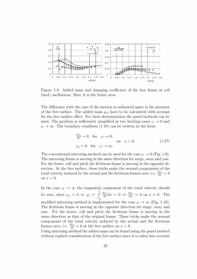
Figure 1.8: Added mass and damping coefficient of the box frame at roll(heel) oscillations. Here A is the frame area.
The difference with the case of the motion in unlimited space is the presenceof the free surface. The added mass µij have to be calculated with accountfor the free surface effect. For their determination the panel methods can beused. The problem is sufficiently simplified in two limiting cases ω → 0 andω →∞. The boundary condition (1.10) can be written in the form:
∂ϕj∂z
= 0 for ω → 0,on z = 0.
ϕj = 0 for ω →∞.(1.27)
The conventional mirroring method can be used for the case ω → 0 (Fig. 1.9).The mirroring frame is moving in the same direction for surge, sway and yaw.For the heave, roll and pitch the fictitious frame is moving in the opposite di-rection. At the free surface, these tricks make the normal components of thetotal velocity induced by the actual and the fictitious frames zero, i.e.
∂ϕj∂z
= 0on z = 0.
In the case ω → ∞ the tangential component of the total velocity should
be zero, since ϕj = 0 ⇒ ϕj =x∫−∞
∂ϕj∂xdx = 0 ⇒ ∂ϕj
∂x= 0 on z = 0. The
modified mirroring method is implemented for the case ω → ∞ (Fig. 1.10).The fictitious frame is moving in the opposite direction for surge, sway andyaw. For the heave, roll and pitch the fictitious frame is moving in thesame direction as that of the original frame. These tricks make the normalcomponents of the total velocity induced by the actual and the fictitiousframes zero, i.e.
∂ϕj∂z
= 0 at the free surface on z = 0.
Using mirroring method the added mass can be found using the panel methodwithout explicit consideration of the free surface since it is taken into account
22
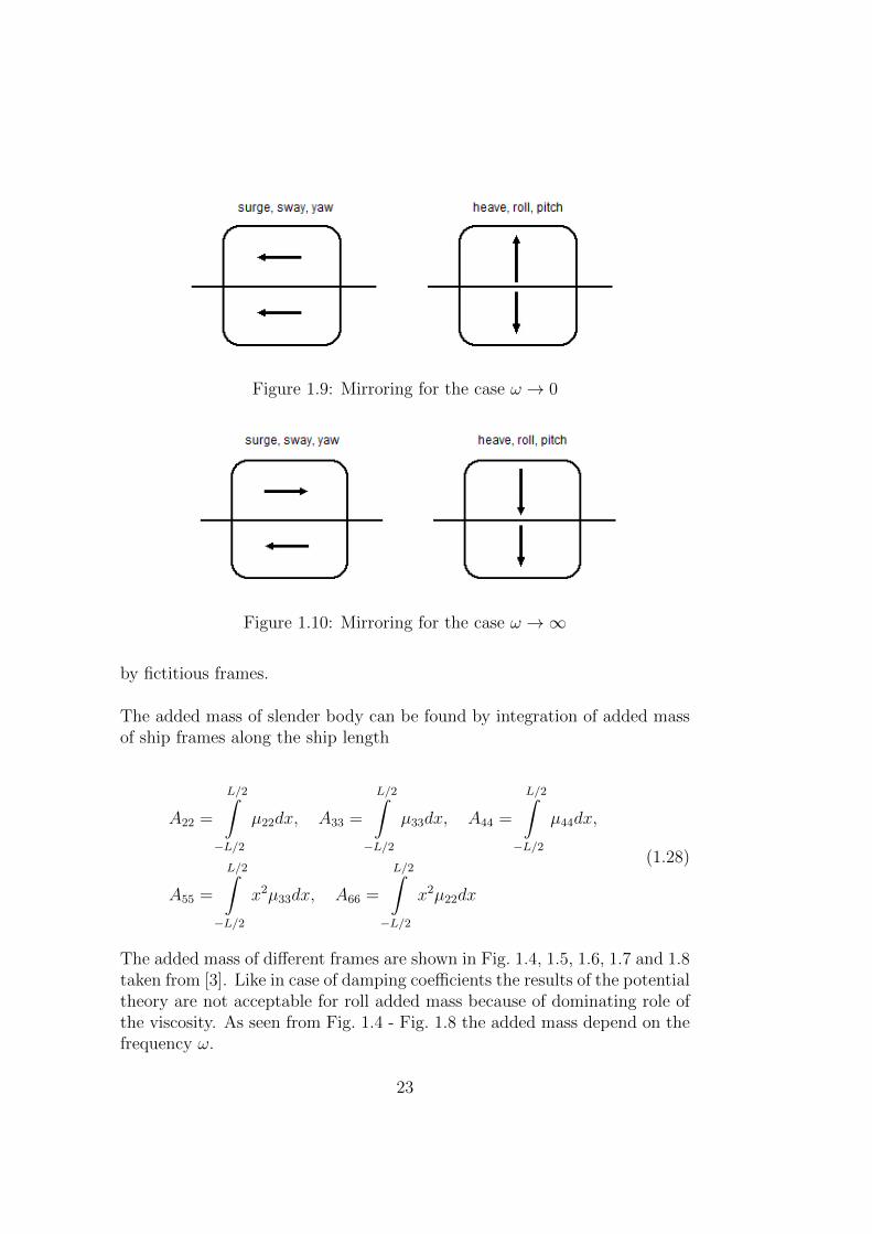
Figure 1.9: Mirroring for the case ω → 0
Figure 1.10: Mirroring for the case ω →∞
by fictitious frames.
The added mass of slender body can be found by integration of added massof ship frames along the ship length
A22 =
L/2∫−L/2
µ22dx, A33 =
L/2∫−L/2
µ33dx, A44 =
L/2∫−L/2
µ44dx,
A55 =
L/2∫−L/2
x2µ33dx, A66 =
L/2∫−L/2
x2µ22dx
(1.28)
The added mass of different frames are shown in Fig. 1.4, 1.5, 1.6, 1.7 and 1.8taken from [3]. Like in case of damping coefficients the results of the potentialtheory are not acceptable for roll added mass because of dominating role ofthe viscosity. As seen from Fig. 1.4 - Fig. 1.8 the added mass depend on thefrequency ω.
23
1.4 Hydrostatic component
Let us the ship is in the equilibrium state. The ship weight is counterbalancedby the hydrostatic lift. Due to small heave motion the equilibrium is violatedand an additional hydrostatic force appears. The vertical component of thisadditional hydrostatic force can be calculated analytically from (1.16) for thecase of small heave motion
∆Fζ =
−ρg∫S
cos(nz)zdS
T+ζ
−
−ρg∫S
cos(nz)zdS
T
= −ρgAWP ζ
(1.29)where ζ is the increment of the ship draught, AWP is the waterplane areaand T is the ship draught in the equilibrium state. The roll and pitch hy-drostatic moments for small change of the roll and pitch angles are
Mϕ = −ρg∇0GMγϕ, (1.30)
Mϑ = −ρg∇0GMLψ, (1.31)
where
ϕ and ψ are the roll and pitch angle respectively,
GMγ is the transverse metacentric height,
GML is the longitudinal metacentric height and
∇0 is the ship displacement.
1.5 Wave exciting force
The wave exciting force ~Fper = ρωA sinωt∫S
~n(ϕ∞+ϕp)dS contains two com-
ponents. The first component, determined by the integration of the incidentpotential ϕ∞, ρωA sinωt
∫S
~nϕ∞dS is referred to as the hydrodynamic part of
the Froude-Krylow force. This force called as the Smith effect is calculated bythe integration of wave induced pressure as if the ship is fully transparent forincident waves. The full Froude-Krylow force contains additionally the hydro-static force arising due to change of the submerged part of the ship caused by
24
waves (the second term in (1.16)). The second component ρωA sinωt∫S
~nϕPdS
takes the diffraction effect (the contribution of the scattering potential ϕp topressure distribution) into account. As shown by Peters and Stokes theFroude Krylov force is a dominating part of the wave induced forces for os-cillations of slender ships in directions j=1 (surge), 3 (heave) and 5 (pitch).
1.6 Motion equations
The linearized decoupled motion equations of the ship oscillations are writtenin the form
added mass damping hydrostatic wave excitingforce forces forces forces
mξ = −A11ξ −B11ξ +Fξ,per(t),mη = −A22η −B22η +Fη,per(t),
mζ = −A33ζ −B33ζ −ρgAWP ζ +Fζ,per(t),Ixxϕ = −A44ϕ −B44ϕ −ρg∇0GMγϕ +Mϕ,per(t),
Iyyψ = −A55ψ −B55ψ −ρg∇0GMLψ +Mψ,per(t),
Izzϑ = −A66ϑ −B66ϑ +Mϑ,per(t).
(1.32)
The weight is not present in the second equation of the system (1.32) be-cause it is counterbalanced by the hydrostatic force at rest. The additionalhydrostatic force −ρgAWP ζ is the difference between the weight and the fullhydrostatic force. The system (1.32) is written in the principle axes coordi-nate system [6].
1.7 Haskind’s relation
One of the most outstanding results in the ship oscillations theory is therelation derived by Max Haskind who developed in 1948 the famous linearhydrodynamic theory of ship oscillations. Haskind shown how to calculatethe wave induced hydrodynamic force utilizing the radiation potentials ϕjand the potential of incident waves ϕ∞. The determination of the diffractionpotential ϕp what is quite difficult can be avoided using this relation whichis valid for waves of arbitrary lengths.
The Green’s formula for two functions Φ and Ψ satisfying the Laplace equa-tion is
25
∫Sw
∫ [Ψ∂Φ
∂n− Φ
∂Ψ
∂n
]dS = 0, (1.33)
where Sw is the flow boundary (wetted ship surface plus the area away fromthe ship, see the sample in Chapter/Section 3.2). Particularly, the rela-tion (1.33) can be applied to radiation potentials ϕj. Since the potential ϕpsatisfies the Laplace equation and the same boundary conditions as the ra-diation potentials ϕj, the Green’s formula (1.33) can also be applied to ϕjand ϕp ∫
Sw
∫ [ϕp∂ϕj∂n− ϕj
∂ϕp∂n
]dS = 0 (1.34)
The last term in (1.16) is the wave induced force
~Fζ,per = ρ(Aω sinωt)
∫S
~n (ϕ∞ + ϕp) dS = ~XA sinωt
where ~X = ρω∫S
~n (ϕ∞ + ϕp) dS. Taking (1.5), (3.34) and (1.8) into account
we get
Xj = ρω
∫Sw
∫(ϕ∞ + ϕp)
∂ϕj∂n
dS (1.35)
∫Sw
∫ϕp
∂ϕj∂ndS =
∫Sw
∫ϕj
∂ϕp∂ndS ⇒ Xj = ρω
∫Sw
∫ (ϕ∞
∂ϕj∂n
+ ϕj∂ϕp∂n
)dS
∂ϕp∂n
= −∂ϕ∞∂n
χ = 90◦
⇓(1.36)
Xj = ρω
∫Sw
∫ (ϕ∞
∂ϕj∂n− ϕj
∂ϕ∞∂n
)dS (1.37)
The formula (1.37) is the Haskind’s relation. As seen the wave induced forcecan be calculated through the radiation and free wave potentials avoidingthe determination of the diffraction potential ϕp.
26
The calculation of the integral (1.37) is a complicated problem because theincident waves don’t decay away from the ship and the integral (1.37) shouldbe calculated over both the surface far from the ship and the ship wettedsurface. Note that the potential ϕ∞ does not decay away from the ship. Themethod of the stationary phase [8] allows one to come to the following forceexpression using the Haskind’s relation (1.37):
Fi,per = Biiζi, where Bii =k
8πρg(c/2)
2π∫0
|Xi(χ)|2dχ
Here c is the phase wave velocity (celerity) and χ is the course angle.
Let us consider the slender ship B(x, z) ∼ 0 in a beam wave (χ = 90◦).The wetted area is approximately equal to the projection on the symmetryplane y = 0, Swetted = [0, L]
⋃[0, T ].
Xj = ρω
∫Sw
∫ (ϕ∞
∂ϕj∂n− ϕj
∂ϕ∞∂n
)dS ≈ ρω
∫Sw
∫ϕ∞
∂ϕj∂n
dS
∂ϕ3
∂n= cos(n, z) =
∂B
∂z⇒ X3 ≈ 2ρωω
∫Sw
∫ϕ∞
∂B
∂zdS
The coefficient 2 arises due to the integration over two boards y = +B(x, z)and y = −B(x, z). Using the potential of an Airy wave (see formulae (6.18)in ([7]) estimated at y = 0 one can find the potential ϕ∞:
ϕ =Ag
ωekz sin(ky − ωt)⇒ ϕ∞ = −gekz/ω
For the case of a vertical cylinder for which the vertical force does not dependon the wave course angle χ the damping coefficient B33 takes a very simpleform [8]:
B33 =2ρg
(c/2)
∣∣∣∣∣∣0∫
−T
ekz∂B
∂zdz
∣∣∣∣∣∣2
(1.38)
1.8 Exercises
1. Schwimmender Balken
27
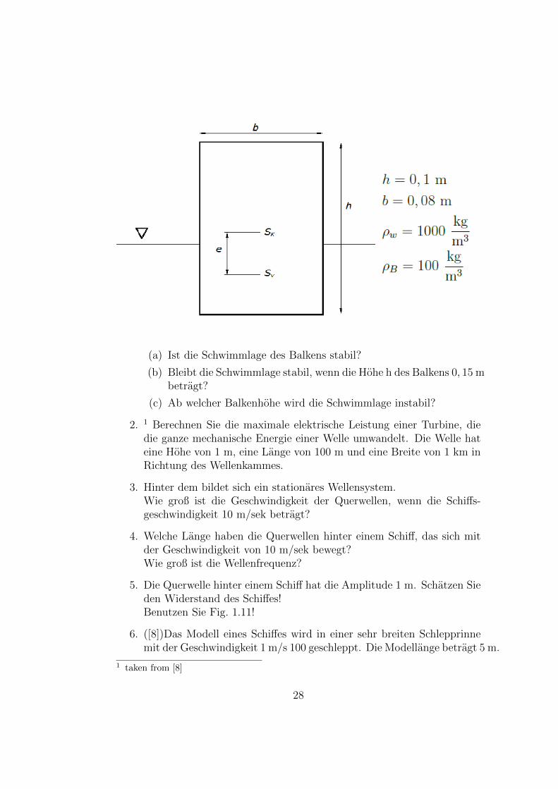
(a) Ist die Schwimmlage des Balkens stabil?
(b) Bleibt die Schwimmlage stabil, wenn die Hohe h des Balkens 0, 15 mbetragt?
(c) Ab welcher Balkenhohe wird die Schwimmlage instabil?
2. 1 Berechnen Sie die maximale elektrische Leistung einer Turbine, diedie ganze mechanische Energie einer Welle umwandelt. Die Welle hateine Hohe von 1 m, eine Lange von 100 m und eine Breite von 1 km inRichtung des Wellenkammes.
3. Hinter dem bildet sich ein stationares Wellensystem.Wie groß ist die Geschwindigkeit der Querwellen, wenn die Schiffs-geschwindigkeit 10 m/sek betragt?
4. Welche Lange haben die Querwellen hinter einem Schiff, das sich mitder Geschwindigkeit von 10 m/sek bewegt?Wie groß ist die Wellenfrequenz?
5. Die Querwelle hinter einem Schiff hat die Amplitude 1 m. Schatzen Sieden Widerstand des Schiffes!Benutzen Sie Fig. 1.11!
6. ([8])Das Modell eines Schiffes wird in einer sehr breiten Schlepprinnemit der Geschwindigkeit 1 m/s 100 geschleppt. Die Modellange betragt 5 m.
1 taken from [8]
28
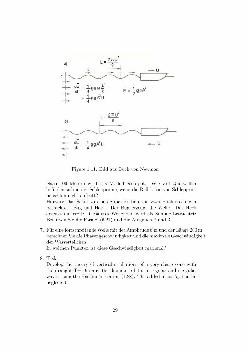
Figure 1.11: Bild aus Buch von Newman
Nach 100 Metern wird das Modell gestoppt. Wie viel Querwellenbefinden sich in der Schlepprinne, wenn die Reflektion von Schlepprin-nenseiten nicht auftritt?Hinweis: Das Schiff wird als Superposition von zwei Punktstorungenbetrachtet: Bug und Heck. Der Bug erzeugt die Welle. Das Heckerzeugt die Welle. Gesamtes Wellenbild wird als Summe betrachtet:Benutzen Sie die Formel (6.21) und die Aufgaben 2 und 3.
7. Fur eine fortschreitende Welle mit der Amplitude 6 m und der Lange 200 mberechnen Sie die Phasengeschwindigkeit und die maximale Geschwindigkeitder Wasserteilchen.In welchen Punkten ist diese Geschwindigkeit maximal?
8. Task:Develop the theory of vertical oscillations of a very sharp cone withthe draught T=10m and the diameter of 1m in regular and irregularwaves using the Haskind’s relation (1.38). The added mass A33 can beneglected.
29

30
Chapter 2
Free oscillations with smallamplitudes
2.1 Theory
Let us consider a ship in the equilibrium position at calm water condition.The ship has zero forward speed. If a perturbation acts on the ship, itperforms oscillating motions in three directions:
• heave,
• roll,
• pitch.
Yaw, surge and sway motions did not arise at calm water conditions. Thereason is the presence of restoring hydrostatic forces in heave, roll and pitchdirections.
The motion equations of the free oscillation read:
(m+ A33) ζ +B33ζ + ρgAWP ζ = 0,
(Ixx + A44) ϕ+B44ϕ+ ρg∇0GMγϕ = 0,
(Iyy + A55) ψ +B55ψ + ρg∇0GMLψ = 0.
(2.1)
In ship theory the equations (2.1) are written in the normalized form:
ζ + 2νζ ζ + ω2ζζ = 0,
ϕ+ 2νϕϕ+ ω2ϕϕ = 0,
ψ + 2νψψ + ω2ψψ = 0,
(2.2)
31
where
νζ =B33
2 (m+ A33), νϕ =
B44
2 (Ixx + A44), νψ =
B55
2 (Iyy + A55)(2.3)
are damping coefficients and
ωζ =
√ρgAWP
m+ A33
, ωϕ =
√ρg∇0GMγ
Ixx + A44
, ωψ =
√ρg∇0GML
Iyy + A55
(2.4)
are the eugen frequencies of non damped oscillations.
The equations (2.2) are fully independent of each other. The solutions of theequations (2.2) written in the general form:
ξ + 2νξ + ω2ξ = 0 (2.5)
is given as:
ξ = Cept (2.6)
Substitution of (2.6) into (2.5) yields the algebraic equation
p2 + 2νp+ ω2 = 0 (2.7)
which solution is
p1,2 = −ν ±√ν2 − ω2 (2.8)
If the system has no damping the solution is
p1,2 = iω → ξ = Ceiωt = C(cosωt+ i sinωt) (2.9)
The system oscillates with the constant amplitude and frequency ω. That iswhy the frequency ω is referred to as the eigenfrequency.
For real ships the damping coefficient is smaller than the eigenfrequency ν � ωand the equation (2.8) has two solutions:
p1 = −ν + i√ω2 − ν2 = −ν + iω,
p2 = −ν − i√ω2 − ν2 = −ν − iω,
(2.10)
32
In turn, the solution of the differential equation is
ξ = Ce−νte±iω = Ce−νt(cos ωt± i sin ωt) (2.11)
It describes damped oscillations with decaying amplitude which decrease isgoverned by the factor e−νt, e−νt −−−→
t→∞0. The rate of the decay is charac-
terized by the damping coefficient ν. The frequency of damped oscillationsis
ω =√ω2 − ν2 < ω (2.12)
Due to damping the frequency of the oscillations is shorter whereas the periodis longer:
T =2π
ω=
2π√ω2 − ν2
(2.13)
Since ω � ν
T =2π
ω=
2π√ω2 − ν2
≈ 2π
ω(2.14)
From (2.12) and (2.14) we obtain the frequencies for different types of oscil-lations which are listed in the table below:
Table 2.1: Frequencies and periods of different oscillation types
Oscillation Eigenfrequency Frequency of Period ofdamped oscillations oscillations
Heave ωζ =√
ρgAWP
m+A33ωζ =
√ω2ζ − ν2
ζ Tζ = 2π√
m+A33
ρgAWP
Rolling ωϕ =√
ρg∇0GMγ
Ixx+A44ωϕ =
√ω2ϕ − ν2
ϕ Tϕ = 2π√
Ixx+A44
ρg∇0GMγ
Pitch ωψ =√
ρg∇0GML
Iyy+A55ωψ =
√ω2ψ − ν2
ψ Tψ = 2π√
Iyy+A55
ρg∇0GML
The damping is characterized by the logarithmic decrement which is thelogarithm of the ratio of the oscillation amplitude at the time instant t tothat at the time instant t+T, i.e.
ξ(t)
ξ(t+ T )=
e−νt
e−ν(t+T )= eνT (2.15)
The logarithm of the ratio (2.15) is
33
lnξ(t)
ξ(t+ T )= ln
e−νt
e−ν(t+T )= lneνT =
2πν
ω(2.16)
The ratio νω
is called as the referred damping factor ν. The decay of the oscil-lation amplitude is equal to this factor multiplied by 2π. Referred dampingfactors for different types of oscillation can be found from this definition.The results obtained under assumption ω � ν are listed in the table 2.2.
If the metacentric heights GMγ and GML are getting larger, the periods Tϕ =
2π√
Ixx+A44
ρg∇0GMγand Tψ = 2π
√Iyy+A55
ρg∇0GMLas well as the damping factors νϕ =
B44
2√
(Ixx+A44)ρg∇0GMγ
and νψ = B55
2√
(Iyy+A55)ρg∇0GML
decrease. Therefore, the
smaller are the metacentric heights the larger are the oscillations periodsand the less oscillations are necessary to decay. The time of decay dependsonly on damping and doesn’t depend on the metacentric height.
Table 2.2: Referred damping factors for different oscillation types
Oscillation Referred damping factor
Heave νζ = B33
2√
(m+A33)ρgAWP
Rolling νϕ = B44
2√
(Ixx+A44)ρg∇0GMγ
Pitch νψ = B55
2√
(Iyy+A55)ρg∇0GML
2.2 Exercise
1. ϕ0 is the roll angle at t = 0. Find the number of periods N of free rolloscillations necessary to reduce the amplitude oscillations by factor ea.What is influence of the metacentric height on N?
2. The period of undamped oscillations is T. The referred damping fac-tor ν is 0,2.Calculate the period of damped oscillations!Calculate the reduction of the amplitude within the period of dampedand undamped oscillations!
3. Typical periods of roll and pitch oscillations for different ships are [9]:Explain why Tϕ > Tψ.
34
Ship Tϕ, sec Tψ, sectanker 9 ... 15 7 ... 11ice breaker 8 ... 12 3 ... 5trawler 6 ... 8 3 ... 4big cruise liner 20 ... 28 10 ... 12container ships (20000− 30000 t) 16 ... 19 7 ... 9
4. The periods of oscillations can be estimated from the following simpleempiric formulae [9]
Tζ ≈ 2.5√T , Tψ ≈ 2.4
√T , Tϑ ≈ cB/
√GMγ,
where T and B are draught and beam. The empiric coefficient c isequal approximately 0, 8...0, 85 for big cruise liners.Calculate the change of the period of roll oscillations of a cruise liner ifa load with mass 1 ton is elevated in vertical direction from 10 m fromthe keel line to the 1 meters from the keel line! The ship displacementis 20 000 t and the beam is 30 m. Use the table from exercise 3 toestimate quantities missed.
35

36
Chapter 3
Ship oscillations in smalltransverse waves (beam see)
The formalism developed in this chapter is based on the following assump-tions:
• waves are regular,
• waves amplitudes related to the wave lengths are small. Wave slope issmall.
• wave length is much larger than the ship width,
• The ship has zero forward speed.
From the first two assumptions it follows, that the collective action of waveson ship can be considered through the superposition principle. Therefore,the theory can be developed for the interaction of the ship with a single wavewith given length and amplitude. The effects of different waves are thensummed. For the case of small waves the oscillations are decoupled. Thehydrodynamic, hydrostatic and gyroscopic coupling effects are neglected.
The perturbation forces (see the last column in the equation system (1.32))arise due to wave induced change of the hydrostatic forces and due to hy-drodynamic effects caused by orbital motion in waves. The orbital motioncauses the hydrodynamic pressure change which results in the wave inducedhydrodynamic forces.
In each frame, the pressure gradient induced by waves is assumed to beconstant along the frame contour and equal to the pressure gradient at the
37
centre A on the free surface. When considering the roll and pitch oscillationsin transverse waves it is additionally assumed that the ship draught change ζand the ship slope relatively to the free surface are constant along the ship.
The wave ordinate is given by the formula derived for the progressive wave(see Chapter 6 in [7])
ζ0 = A sin (ωt+ kχ) (3.1)
where A is the amplitude, χ is the wave propagation direction and ω is thefrequency.
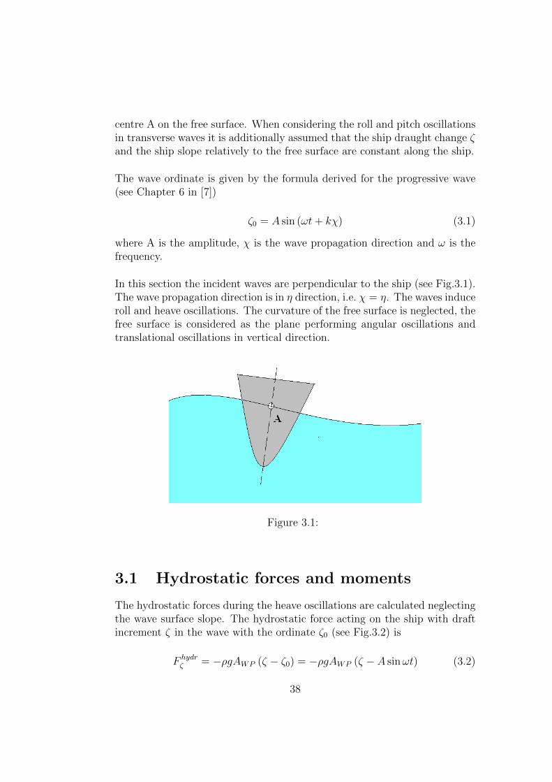
In this section the incident waves are perpendicular to the ship (see Fig.3.1).The wave propagation direction is in η direction, i.e. χ = η. The waves induceroll and heave oscillations. The curvature of the free surface is neglected, thefree surface is considered as the plane performing angular oscillations andtranslational oscillations in vertical direction.
Figure 3.1:
3.1 Hydrostatic forces and moments
The hydrostatic forces during the heave oscillations are calculated neglectingthe wave surface slope. The hydrostatic force acting on the ship with draftincrement ζ in the wave with the ordinate ζ0 (see Fig.3.2) is
F hydrζ = −ρgAWP (ζ − ζ0) = −ρgAWP (ζ − A sinωt) (3.2)
38

where η = 0 at the point A. Since the wave slope is neglected, the de-pendence of ζ0 on ζ is not considered. The first part −ρgAWP ζ is therestoring hydrostatic force which is already present in (1.32). The secondpart ρgAWPA sinωt is the wave induced hydrostatic force.
Figure 3.2: Illustration of hydrostatic force
The additional hydrostatic moment is determined from the analysis of theFigure 3.3.
Figure 3.3: Illustration of hydrostatic moment
The relative slope of the ship to the free surface is ϕ−α, where α is the wavesurface slope
39
α =dζ0
dη
∣∣∣∣η−0
= Ak cosωt =ω2
gA cosωt = αA cosωt (3.3)
αA is the amplitude of the angular water plane oscillations. The hydrostaticpressure increases linearly in direction perpendicular to the free surface plane.Therefore, the restoring moment is the same as in the case if the free surface ishorizontal and the ship is inclined at the angle ϕ−α. The restoring momentis known from the ship hydrostatics
Mhydrϕ = −ρg∇0GMγ(ϕ− α) = −ρg∇0GMγ(ϕ− αA cosωt) (3.4)
The first part −ρg∇0GMγϕ is the restoring hydrostatic moment, whereas thesecond part ρg∇0GMγαA cosωt is the wave induced hydrostatic moment.
3.2 Hydrodynamic Krylov - Froude force
Hydrodynamic forces arise due to wave induced hydrodynamic pressures.From the Bernoulli equation the pressure is (see (1.13)).
p = −ρu2
2− ρgz − ρ∂ϕ
∂t+ pa (3.5)
The constant pressure pa does not need to be considered since being inte-grated over the ship wetted surface results in zero force and moment. Thefirst term in (3.5) is neglected within the linear theory under consideration.The second term results in force and moment considered above in the sec-tion 3.1. The remaining term punst = −ρ∂ϕ
∂tis responsible for hydrodynamic
effects caused by waves. If the interaction between the ship and incidentwaves is neglected (Krylov - Froude formalism) the potential can be writtenas the potential of uniform unsteady parallel flow:
ϕ = uζ(t)ζ (3.6)
where uζ(t) is unsteady velocity of the flow in the wave
uζ(t) =dζ0
dt(3.7)
Since the unsteady pressure punst = −ρ∂ϕ∂t
= −ρζ ∂uζ∂t
is zero at ζ = 0 thetotal pressure is equal to the atmospheric pressure p = pa (see (3.5)). Thegradient of the hydrodynamic pressure in vertical direction reads:
40
∂punst∂ζ
= −ρ ∂∂ζ
(∂ϕ
∂t
)= −ρ ∂
∂t
(∂ϕ
∂ζ
)= −ρ∂uζ(t)
∂t= −ρζ0 = ρω2A sinωt
(3.8)
The unsteady pressure at the point ζ is then:
punst(ζ) = punst(ζ = 0) +
ζ∫0
∂punst
∂zdz =
ζ∫0
∂punst
∂zdz
The force caused by punst on each frame is calculated by the integration ofthe pressure over the frame wetted area
dF dynζ =
∮punst cos(nζ)dC =
∮ ζ∫0
∂punst
∂zdz
cos(nζ)dC =
=
∮ ζ∫0
ρω2A sinωtdz
cos(nζ)dC = ρω2A sinωt
∮ζ cos(nζ)dC
(3.9)
Here the normal vector is the inward normal vector.Since the integral
∮ζ cos(nζ)dC is equal to the frame area taken with the
opposite sign, i.e. −Af , the hydrodynamic force caused by waves takes theform:
dF dynζ = −ρω2A sinωtAf (3.10)
Being integrated along the ship length this force gives the force acting on thewhole ship length
F dynζ =
L∫0
dF dynζ dξ = −
L∫0
ρω2A sinωtAfdξ =
= −ω2A sinωt
L∫0
ρAfdξ = −mω2A sinωt = mζ0
(3.11)
The hydrodynamic moment acting on the ship frame
41
dMdynϕ =
∮punst(η cos(nζ)− ζ cos(nη))dC =
= ρω2A sinωt
∮ζ(η cos(nζ)− ζ cos(nη))dC
(3.12)
Within the linear theory considering small ship slopes the last integral in (3.12)is zero, i.e.
dMdynϕ = 0→Mdyn
ϕ =
L∫0
dMdynϕ = 0 (3.13)
3.3 Full Krylov - Froude force and moment
The full Froude Krylov force takes the form:
F lζ = ρgAWPA sinωt−mω2A sinωt = ρgAWPA sinωt+mζ0 (3.14)
The first term is caused by hydrostatic effect, whereas the second one byhydrodynamic effects. The second term is referred in the literature to as theSmith effect.The full Froude Krylov moment contains only the wave induced hydrostaticcomponent:
M lϕ = ρg∇0GMγαA cosωt (3.15)
3.4 Force and moment acting on the ship frame
in accelerated flow
These forces are determined using the concept of the relative motion. Letus ζj is a ship displacement in j-th direction. As it has been explained in pre-vious chapters, the force acting on the body moving with the acceleration ζjin a liquid at rest is equal to the product of added mass with the accelerationtaken with opposite sign, i.e. −Ajj ζj. If the liquid moves with the accelera-tion ζjL relative to motionless body, the force acting on the body is towardsthe acceleration direction, i.e. Ajj ζjL. If both body and liquid move with ac-celerations the total force is −Ajj(ζj− ζjL). Similarly, the damping force canintroduced being proportional to the relative velocity −Bjj(ζj − ζjL). The
42
first components of both forces −Ajj ζj and −Bjj ζj are already representedby the first and the second columns in the motion equations (1.32). The sec-ond components Ajj ζjL and Bjj ζjL represent the hydrodynamic forces dueto interaction between the incident waves and floating body. Rememberingthat ζjL = ωA cosωt and ζjL = −ω2A sinωt we obtain the lift force causedby the interaction between the ship and incident wave:
F 2ζ = −A33ω
2A sinωt+B33ωA cosωt (3.16)
In roll oscillations the ship moves with the angular velocity ϕ and angularacceleration ϕ. The free surface oscillates with the angular velocity α andacceleration α. Taking α from (3.3) we obtain the roll moment caused bythe interaction between the ship and incident wave:
M2ϕ = −A44ω
2αA cosωt−B44ωαA sinωt = −A44ω4
gA cosωt−B44
ω3
gA sinωt
(3.17)
3.5 Full wave induced force and moment
In the section 1.5 we divided the wave induced forces into the Froude Krylovpart and the interaction force. Commonly, the Froude Krylov force is thedominating part of the wave induced forces.
To calculate the full wave induced force we have to note that the Smith effectis already represented in the force Ajj ζjL +Bjj ζjL. All hydrodynamic effectsare taken into account. Only the hydrostatic part of the Froude Krylov forceshould be added to Ajj jL+Bjj ζjL to get the full wave induced force:
Fζ,per =[ρgAWP − ω2A33
]A sinωt+B33ωA cosωt (3.18)
The full moment is the sum of (3.15) and (3.17):
Mϕ,per =(ρg∇0GMγ − A44ω
2) ω2
gA cosωt−B44
ω3
gA sinωt (3.19)
3.6 Equations of ship heave and roll oscilla-
tions
Substitution of all forces derive above into the original differential equationsresults in two following decoupled ordinary differential equations
43
(m+ A33)(ζ − ζ0
)+B33
(ζ − ζ0
)+ ρgAWP (ζ − ζ0) = −mζ0 (3.20)
(Ixx + A44) (ϕ− α) +B44 (ϕ− α) + ρg∇0GMγ (ϕ− α) = −Ixxα. (3.21)
The solution of both equations can be represented as the sum ζ = ζinh+ζfreeϕ = ϕinh + ϕfree, where ζfree and ϕfree are free heave and roll oscillations:ϕfree = Ce−νϕt (cos ωϕt± i sin ωϕt), ζfree = Ce−νζt (cos ωζt± i sin ωζt) satis-fying the homogeneous equations:
(m+ A33) ζ +B33ζ + ρgAWP ζ = 0
(Ixx + A44) ϕ+B44ϕ+ ρg∇0GMγϕ = 0.
When the free oscillations decay ϕfree, ζfree −−−→t→∞
0, the solutions of the
equation (3.20) and (3.21) tend to the solutions of inhomogeneous equations:
(m+ A33) ζ +B33ζ + ρgAWP ζ = A33ζ0 +B33ζ0 + ρgAWP ζ0
(Ixx + A44) ϕ+B44ϕ+ ρg∇0GMγϕ = A44α +B44α + ρg∇0GMγα.(3.22)
The inhomogeneous equation (3.21) is written in terms of relative roll an-gle ϕ(r) = ϕ− α in the normalized form:
ϕ(r) + 2νϕϕ(r) + ω2
ϕϕ(r) =
ω2
1 + kϕαA cosωt, (3.23)
where kϕ = A44/Ixx. The solution of (3.23) is seeking in the form
ϕ(r) = ϕ(r)A cos (ωt− δϕ) (3.24)
Substituting (3.24) into (3.23) and separating terms proportional to cosωtand sinωt gives two equations:
ϕ(r)A
[(ω2
ϕ − ω2) cos δϕ + 2νϕω sin δϕ]
=ω2
1 + kϕαA (3.25)
ϕ(r)A
[−2νϕω cos δϕ + (ω2
ϕ − ω2) sin δϕ]
= 0 (3.26)
It follows from (3.25) and (3.26)
44
(ϕ
(r)A
)2 [(ω2ϕ − ω2
)2cos2 δϕ + 4ν2
ϕω2 sin2 δϕ+
+4νϕω sin δϕ(ω2ϕ − ω2
)cos δϕ
]=
ω4
(1 + kϕ)2α2A(
ϕ(r)A
)2 [(ω2ϕ − ω2
)2sin2 δϕ + 4ν2
ϕω2 cos2 δϕ−
−4νϕω cos δϕ(ω2ϕ − ω2
)sin δϕ
]= 0.
The sum of two last equations
(ϕ
(r)A
)2 [(ω2ϕ − ω2
)2+ 4ν2
ϕω2]
=ω4
(1 + kϕ)2α2A
allows one to find the ratio ϕ(r)A /αA
ϕ(r)A
αA=
ω2ϕ/ (1 + kϕ)√(
1− ω2ϕ
)2+ 4ν2
ϕω2ϕ
, (3.27)
where ωϕ = ωωϕ
and νϕ = νϕωϕ
1. Eigenfrequency ωϕ and damping coefficient νϕare given by formulae (2.3) and (2.4). The phase of the response relative tothat of the input (phase displacement) is found from (3.26):
δϕ = arctan
(2νϕωϕ1− ω2
ϕ
)(3.28)
Similar solutions are obtained for the heave oscillations:
ζ(r)A
A=
ω2ζ/(1 + kζ)√
(1− ω2ζ )
2 + 4ν2ζ ω
2ζ
(3.29)
δζ = arctg
(2νζωζ1− ω2
ζ
)(3.30)
with kζ = A33/m, ωζ = ωωζ
and νζ =νζωζ
.
1 since ω � ν, νϕ ≈ νϕ introduced in table 2.2
45
3.7 Analysis of the formula (3.27)
The formula (3.27) can be rewritten as follows:
ϕ(r)A
αA=ϕA − αAαA
=ω2ϕ/ (1 + kϕ)√(
1− ω2ϕ
)2+ 4ν2
ϕω2ϕ
or
ϕAαA
= 1 +ω2ϕ/ (1 + kϕ)√(
1− ω2ϕ
)2+ 4ν2
ϕω2ϕ
(3.31)
The physical meaning of terms in (3.31) is obvious from the following expres-sion
amplitude of ship roll oscillations
amplitude of wave angle oscillations= 1 + enhancement (3.32)
Since the functionω2ϕ/(1+kϕ)√
(1−ω2ϕ)
2+4ν2ϕω
2ϕ
is positiveω2ϕ/(1+kϕ)√
(1−ω2ϕ)
2+4ν2ϕω
2ϕ
> 0 the ship
roll amplitude is larger than the the amplitude of the angular water planeoscillations αA, i.e. ϕA
αA> 1.
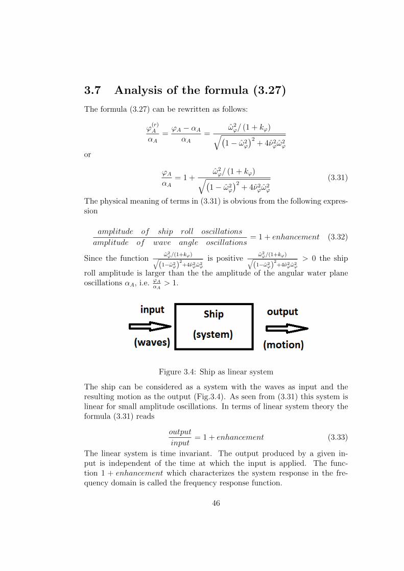
Figure 3.4: Ship as linear system
The ship can be considered as a system with the waves as input and theresulting motion as the output (Fig.3.4). As seen from (3.31) this system islinear for small amplitude oscillations. In terms of linear system theory theformula (3.31) reads
output
input= 1 + enhancement (3.33)
The linear system is time invariant. The output produced by a given in-put is independent of the time at which the input is applied. The func-tion 1 + enhancement which characterizes the system response in the fre-quency domain is called the frequency response function.
46
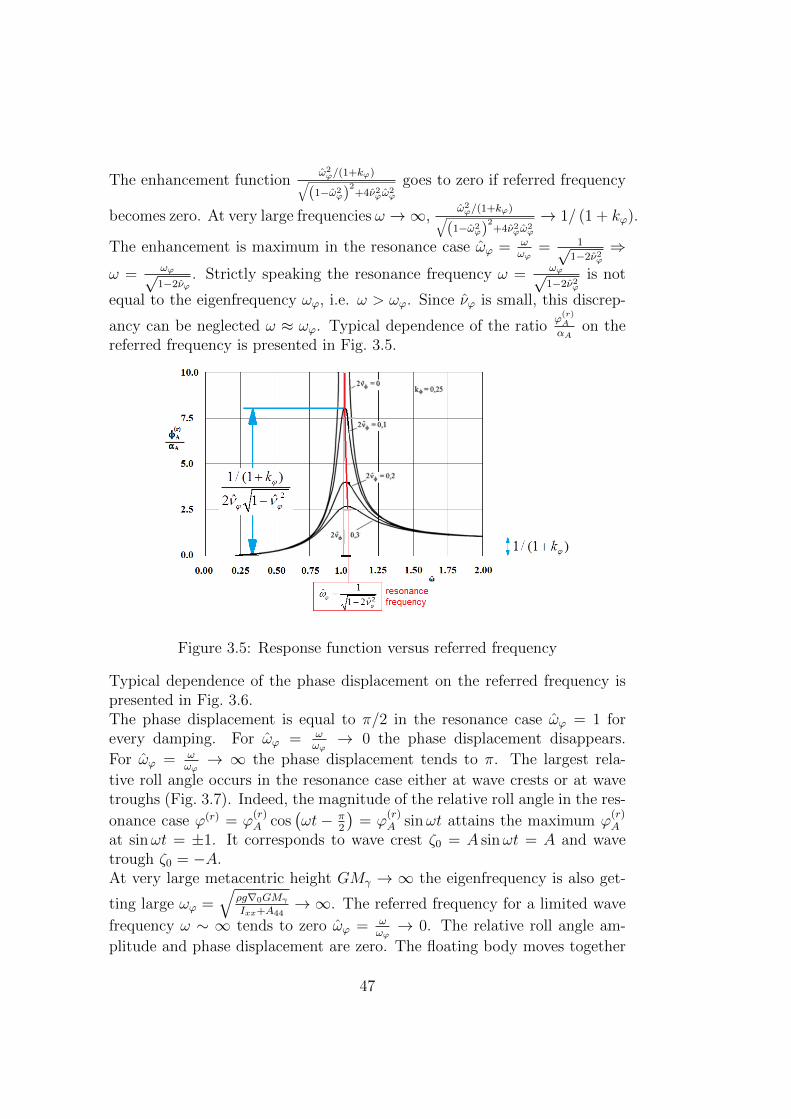
The enhancement functionω2ϕ/(1+kϕ)√
(1−ω2ϕ)
2+4ν2ϕω
2ϕ
goes to zero if referred frequency
becomes zero. At very large frequencies ω →∞,ω2ϕ/(1+kϕ)√
(1−ω2ϕ)
2+4ν2ϕω
2ϕ
→ 1/ (1 + kϕ).
The enhancement is maximum in the resonance case ωϕ = ωωϕ
= 1√1−2ν2ϕ
⇒
ω = ωϕ√1−2νϕ
. Strictly speaking the resonance frequency ω = ωϕ√1−2ν2ϕ
is not
equal to the eigenfrequency ωϕ, i.e. ω > ωϕ. Since νϕ is small, this discrep-
ancy can be neglected ω ≈ ωϕ. Typical dependence of the ratioϕ(r)A
αAon the
referred frequency is presented in Fig. 3.5.
Figure 3.5: Response function versus referred frequency
Typical dependence of the phase displacement on the referred frequency ispresented in Fig. 3.6.The phase displacement is equal to π/2 in the resonance case ωϕ = 1 forevery damping. For ωϕ = ω
ωϕ→ 0 the phase displacement disappears.
For ωϕ = ωωϕ→ ∞ the phase displacement tends to π. The largest rela-
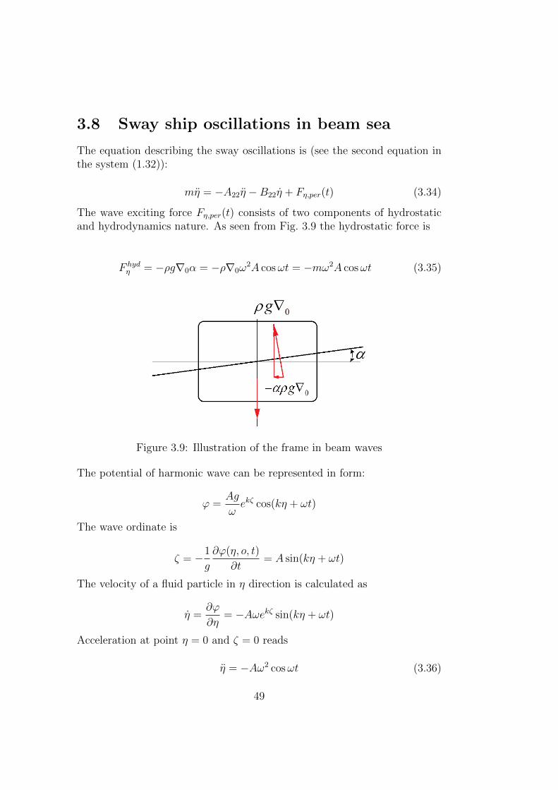
tive roll angle occurs in the resonance case either at wave crests or at wavetroughs (Fig. 3.7). Indeed, the magnitude of the relative roll angle in the res-
onance case ϕ(r) = ϕ(r)A cos
(ωt− π
2
)= ϕ
(r)A sinωt attains the maximum ϕ
(r)A
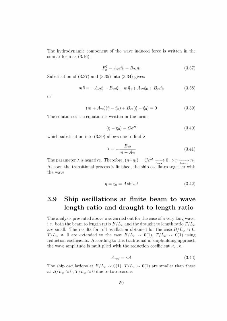
at sinωt = ±1. It corresponds to wave crest ζ0 = A sinωt = A and wavetrough ζ0 = −A.At very large metacentric height GMγ → ∞ the eigenfrequency is also get-
ting large ωϕ =√
ρg∇0GMγ
Ixx+A44→∞. The referred frequency for a limited wave
frequency ω ∼ ∞ tends to zero ωϕ = ωωϕ→ 0. The relative roll angle am-
plitude and phase displacement are zero. The floating body moves together
47
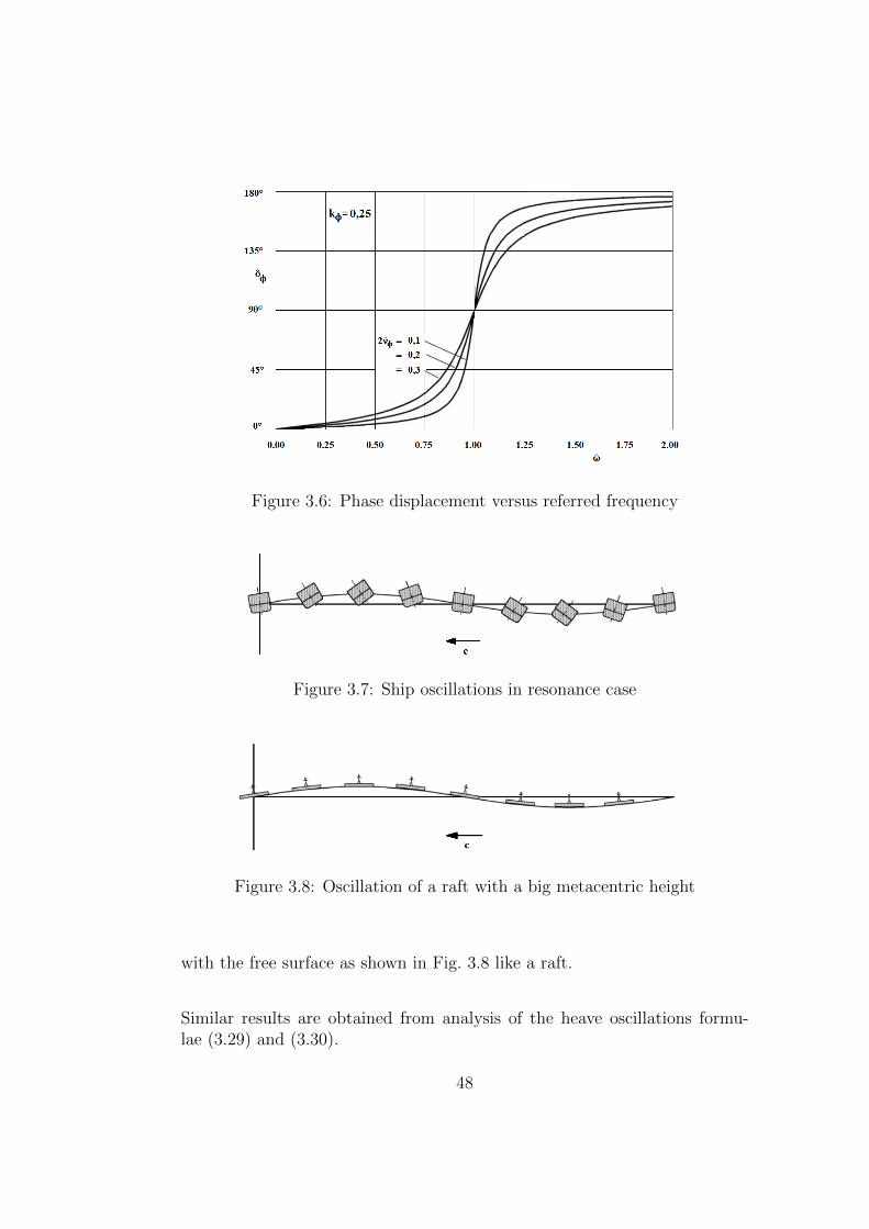
Figure 3.6: Phase displacement versus referred frequency
Figure 3.7: Ship oscillations in resonance case
Figure 3.8: Oscillation of a raft with a big metacentric height
with the free surface as shown in Fig. 3.8 like a raft.
Similar results are obtained from analysis of the heave oscillations formu-lae (3.29) and (3.30).
48
3.8 Sway ship oscillations in beam sea
The equation describing the sway oscillations is (see the second equation inthe system (1.32)):
mη = −A22η −B22η + Fη,per(t) (3.34)
The wave exciting force Fη,per(t) consists of two components of hydrostaticand hydrodynamics nature. As seen from Fig. 3.9 the hydrostatic force is
F hydη = −ρg∇0α = −ρ∇0ω
2A cosωt = −mω2A cosωt (3.35)
Figure 3.9: Illustration of the frame in beam waves
The potential of harmonic wave can be represented in form:
ϕ =Ag
ωekζ cos(kη + ωt)
The wave ordinate is
ζ = −1
g
∂ϕ(η, o, t)
∂t= A sin(kη + ωt)
The velocity of a fluid particle in η direction is calculated as
η =∂ϕ
∂η= −Aωekζ sin(kη + ωt)
Acceleration at point η = 0 and ζ = 0 reads
η = −Aω2 cosωt (3.36)
49
The hydrodynamic component of the wave induced force is written in thesimilar form as (3.16):
F 2η = A22η0 +B22η0 (3.37)
Substitution of (3.37) and (3.35) into (3.34) gives:
mη = −A22η −B22η +mη0 + A22η0 +B22η0 (3.38)
or
(m+ A22)(η − η0) +B22(η − η0) = 0 (3.39)
The solution of the equation is written in the form:
(η − η0) = Ceλt (3.40)
which substitution into (3.39) allows one to find λ
λ = − B22
m+ A22
(3.41)
The parameter λ is negative. Therefore, (η−η0) = Ceλt −−−→t→∞
0⇒ η −−−→t→∞
η0.
As soon the transitional process is finished, the ship oscillates together withthe wave
η = η0 = A sinωt (3.42)
3.9 Ship oscillations at finite beam to wave
length ratio and draught to length ratio
The analysis presented above was carried out for the case of a very long wave,i.e. both the beam to length ratioB/Lw and the draught to length ratio T/Lware small. The results for roll oscillation obtained for the case B/Lw ≈ 0,T/Lw ≈ 0 are extended to the case B/Lw ∼ 0(1), T/Lw ∼ 0(1) usingreduction coefficients. According to this traditional in shipbuilding approachthe wave amplitude is multiplied with the reduction coefficient κ, i.e.
Ared = κA (3.43)
The ship oscillations at B/Lw ∼ 0(1), T/Lw ∼ 0(1) are smaller than theseat B/Lw ≈ 0, T/Lw ≈ 0 due to two reasons
50
• Hydrostatic force is smaller because the submerged volume is smallerdue to wave surface curvature,
• Hydrodynamic force is smaller because the velocities caused by theorbital motion are not constant as assumed above. They decay withthe increasing submergence as ∼ exp(−kz).
The first reduction factor is mainly due to the finite beam to length ra-tio B/Lw ∼ 0(1).
Let us consider first the reduction coefficient for the heave oscillations. Thefactor κBζ considers the reduction of the hydrostatic force due to the finitebeam to length ratio. To estimate κBζ the fixed ship is considered at the timeinstant ωt = π/2 when the wave crest is in the symmetry plane (Fig. 3.10).
Figure 3.10:
The free surface ordinate
ζ0 = A sin(π
2+ kη
)= A cos kη
The hydrostatic force obtained in the previous analysis is
R0 = ρgAAwp (3.44)
whereas the actual one is calculated by the integral:
51
Rtrue = ρgA
∫Awp
cos kηdξdη = 2ρgA
L/2∫−L/2
B(ξ)/2∫0
cos kηdηdξ =
=2ρgA
k
L/2∫−L/2
sinkB(ξ)
2dξ
(3.45)
Using the Taylor expansion for sin kB(ξ)
sinkB(ξ)
2=kB
2− (kB)3
48+ ...
the final formula for Rtrue takes the form:
Rtrue =2ρgA
k
L/2∫−L/2
sinkB(ξ)
2dξ ≈ 2ρgA
k
L/2∫−L/2
(kB/2− (kB)3
48
)dξ =
= ρgAAwp −ρgAk2
24
L/2∫−L/2
B3dξ = ρgAAwp
(1− k2
2
I
Awp
),
(3.46)
where
Awp =
L/2∫−L/2
Bdξ, I =1
12
L/2∫−L/2
B3dξ,
The reduction of the hydrostatic force can be taken by the following coeffi-cient into account:
κBζ =ρgAAwp
(1− k2
2I
Awp
)ρgAAwp
= 1− k2
2
I
Awp(3.47)
The second reduction factor is mainly due to the finite draught to length ra-tio T/Lw ∼ 0(1). The factor κTζ considers the reduction of the hydrodynamicforce due to the finite draught to length ratio. The reduction coefficient isgiven here without derivation:
κTζ = 1− χ(
2πT
Lw
)+
χ
2(2− χ)
(2π
T
Lw
)2
− χ
6(3− 2χ)
(2π
T
Lw
)3
(3.48)
52
where χ is the coefficient of the lateral area χ = ALA/(LT ).The total reduction coefficient κζ is calculated as the product of κBζ and κTζneglecting their mutual influence:
κζ = κBζκTζ (3.49)
The formula (3.49) is valid at LwB> 4, Lw
T> 8. For heave calculations one
can use the formula (3.29) with Aκζ instead of A.
Reduction coefficient of the roll oscillations can be calculated from the ex-pression gained from regression of experimental data:
κϕ = exp(−4.2 (Rωϕ)2) , R = χωϕ
[√BTχrγ/GMγ
2πg
]1/2
(3.50)
Here rγ is the metacentric radius. Amplitude of roll oscillations is foundfrom (3.31) with αAκϕ instead of αA. A sample of the reduction coefficientfor a real ship is presented in Fig. 3.11.
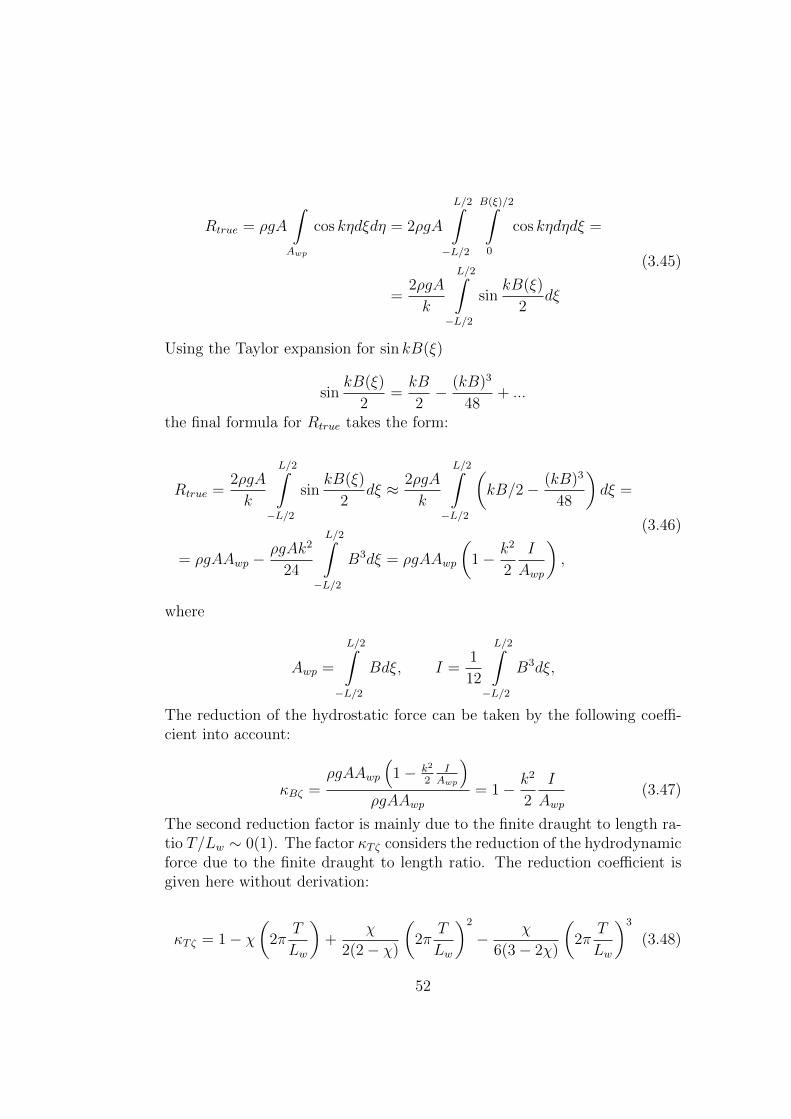
Figure 3.11: Reduction coefficient of the heave oscillations
3.10 Effect of ship speed on rolling
In the previous chapters the ship speed was assumed to be zero. If the shipmoves in waves with speed v in x-direction the following modifications should
53
be made in theory
• the added mass Aij and damping coefficients Bij depend on the en-counter frequency
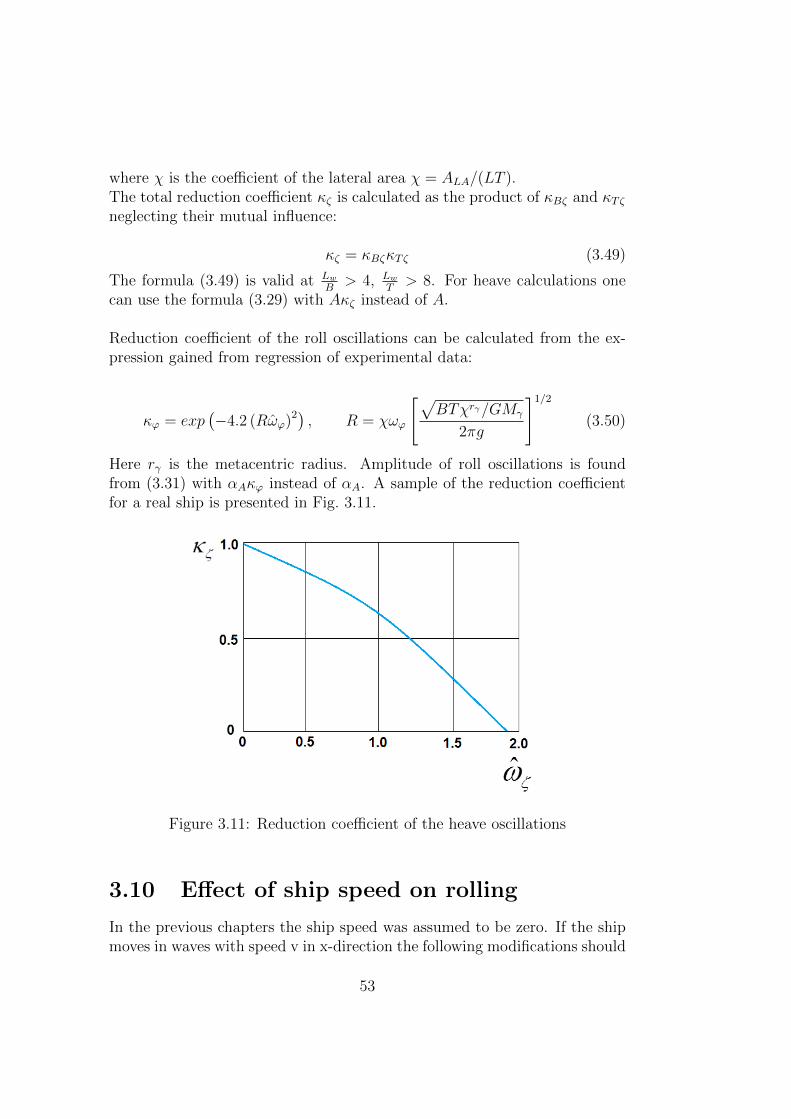
ωe = ω − ω2v cosϕwaveg
where ϕwave is encounter angle (Fig. 3.12)
Figure 3.12: Sea classification
• reduction coefficient κ (3.43) depends on ω
• In the hydrodynamic theory one uses time derivative in ship coordinatesystem ∂ϕ
∂twhich can be expressed through the time derivative in the
inertial reference system ∂ϕ∂t0
as
∂ϕ
∂t0=∂ϕ
∂t− ~v∇ϕ
54

The formulae (3.27 - 3.30) can be used also in the case v 6= 0 with thesubstitution ωe instead of ω.
55

56
Chapter 4
Ship oscillations in small headwaves
4.1 Exciting forces and ship oscillations
Let us consider the ship oscillations in small head waves coming from thestern (ψwave = 0◦), where ψwave is the wave course angle. The wave ordinate,wave orbital motion velocity and acceleration are:
ζ0 = A sin(ωt− kξ) (4.1)
ζ0 = ωA cos(ωt− kξ) (4.2)
ζ0 = −ω2A sin(ωt− kξ) (4.3)
Figure 4.1: Illustration of the ship in head waves
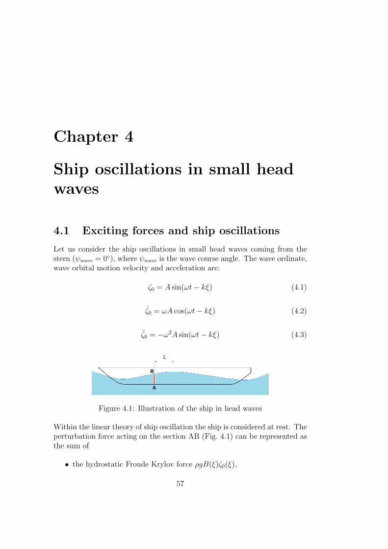
Within the linear theory of ship oscillation the ship is considered at rest. Theperturbation force acting on the section AB (Fig. 4.1) can be represented asthe sum of
• the hydrostatic Froude Krylov force ρgB(ξ)ζ0(ξ),
57
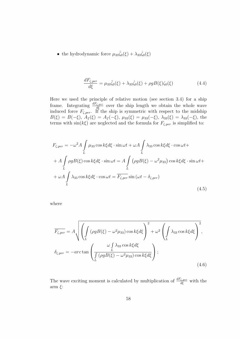
• the hydrodynamic force µ33ζ0(ξ) + λ33ζ0(ξ)
dFζ,perdξ
= µ33ζ0(ξ) + λ33ζ0(ξ) + ρgB(ξ)ζ0(ξ) (4.4)
Here we used the principle of relative motion (see section 3.4) for a ship
frame. IntegratingdFζ,perdξ
over the ship length we obtain the whole waveinduced force Fζ,per. If the ship is symmetric with respect to the midshipB(ξ) = B(−ξ), Af (ξ) = Af (−ξ), µ33(ξ) = µ33(−ξ), λ33(ξ) = λ33(−ξ), theterms with sin(kξ) are neglected and the formula for Fζ,per is simplified to:
Fζ,per = −ω2A
∫L
µ33 cos kξdξ · sinωt+ ωA
∫L
λ33 cos kξdξ · cosωt+
+ A
∫L
ρgB(ξ) cos kξdξ · sinωt = A
∫L
(ρgB(ξ)− ω2µ33
)cos kξdξ · sinωt+
+ ωA
∫L
λ33 cos kξdξ · cosωt = Fζ,per sin (ωt− δζ,per)
(4.5)
where
Fζ,per = A
√√√√√∫L
(ρgB(ξ)− ω2µ33) cos kξdξ
2
+ ω2
∫L
λ33 cos kξdξ
2
,
δζ,per = −arc tan
ω∫L
λ33 cos kξdξ∫L
(ρgB(ξ)− ω2µ33) cos kξdξ
;
(4.6)
The wave exciting moment is calculated by multiplication ofdFζ,perdξ
with thearm ξ:
58
Mψ,per = −∫L
ξdFE,ζdξ
dξ
= A
∫L
(ρgB(ξ)− ω2µ33
)ξ sin kξ · cosωt−
− ωA∫L
λ33ξ sin kξ · sinωt = Mψ,per sin (ωt− δψ,per)
(4.7)
where
Mψ,per = A
√√√√√∫L
(ρgB(ξ)− ω2µ33) ξ sin kξdξ
2
+ ω2
∫L
λ33ξ sin kξdξ
2
,
δψ,per = −π + arc tan
∫L
(ρgB(ξ)− ω2µ33) ξ sin kξdξ
ω∫L
λ33ξ sin kξdξ
;
(4.8)
Substitution (4.5) and (4.7) in the third and sixth equations of the sys-tem (1.3.2) gives:
mζ = −A33ζ −B33ζ − ρgAWP ζ + Fζ,per sin (ωt− δζ,per) (4.9)
Iyyψ = −A55ψ −B55ψ − ρg∇0GMLψ +Mψ,per sin (ωt− δψ,per) (4.10)
⇓
(m+ A33) ζ +B33ζ + ρgAWP ζ = Fζ,per sin (ωt− δζ,per) (4.11)
(Iyy + A55) ψ +B55ψ + ρg∇0GMLψ = Mψ,per sin (ωt− δψ,per) (4.12)
Note that A33, B33 are the coefficients for the whole ship, whereas µ33 andλ33 for ship frames.Dividing both equations by the coefficient of the first term one obtains:
59
ζ + 2νζ ζ + ω2ζζ = fζ sin (ωt− δζ,per)
ψ + 2νψψ + ω2ψψ = fψ sin (ωt− δψ,per)
(4.13)
where
fζ =Fζ,per
m+ A33
, fψ =Mψ,per
Iyy + A55
, νζ =B33
2(m+ A33), νψ =
B55
2(Iyy + A55),
ωζ =
√ρgAWP
m+ A33
, ωψ =
√ρg∇0GML
Iyy + A55
.
Solution of (4.13) is seeking in the form
ζ = ζA sin(ωt− δζ,per − δperζ
), ψ = ψA sin
(ωt− δψ,per − δperψ
). (4.14)
Using trigonometric formulae sin(ωt−δζ,per−δperζ ) = sin(ωt−δζ,per) cos δperζ −cos(ωt− δζ,per) sin δperζ one gets for the first equation of (4.13)
ξA = ((ω2ζ − ω2) cos δperζ + 2νζω sin δperζ ) sin(ωt− δζ,per)
− ξA((ω2ζ − ω2) sin δperζ − 2νζω cos δperζ ) cos(ωt− δζ,per) =
= fζ sin(ωt− δζ,per).(4.15)
This equation is splitted into two following equations:
ζA((ω2ζ − ω2) cos δperζ + 2µζω sin δperζ ) = fζ
ξA((ω2ζ − ω2) sin δperζ − 2νζω cos δperζ ) = 0
Squaring two last equations and summing them one obtains:
ζ2A(ω2
ζ − ω2)2 + 4ν2ζω
2 = f 2ζ
and
ζA =fζ√
(ω2ζ − ω2)2 + 4ν2
ζω2
The phase displacement δperζ is found from the second equation
60
δperζ = arctan
(2νζω
ω2ζ − ω2
)Similarly one gets the solution for pitch:
ψA =fψ√
(ω2ψ − ω2)2 + 4ν2
ψω2, δperψ = arc tan
(2νψω
ω2ψ − ω2
)(4.16)
In the resonance case the phase displacement is equal to π/2, i.e.δperζ = π/2 in case ωζ = ω and δperψ = π/2 in case ωψ = ω.
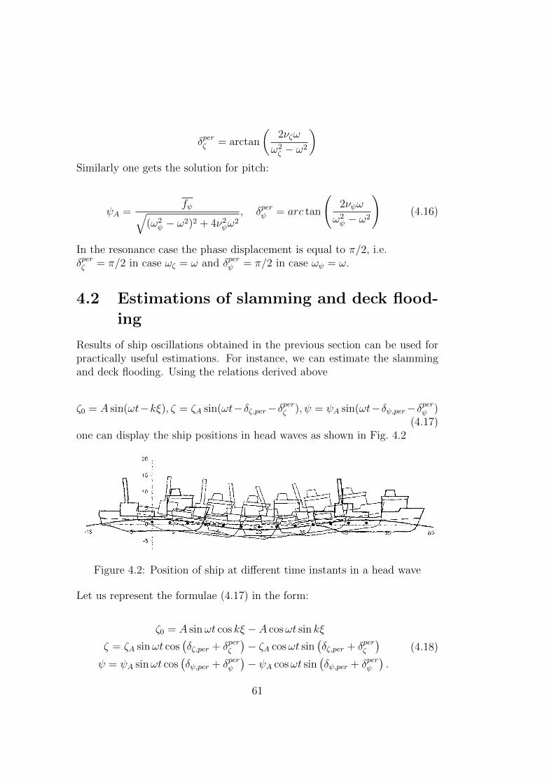
4.2 Estimations of slamming and deck flood-
ing
Results of ship oscillations obtained in the previous section can be used forpractically useful estimations. For instance, we can estimate the slammingand deck flooding. Using the relations derived above
ζ0 = A sin(ωt−kξ), ζ = ζA sin(ωt−δζ,per−δperζ ), ψ = ψA sin(ωt−δψ,per−δperψ )(4.17)
one can display the ship positions in head waves as shown in Fig. 4.2
Figure 4.2: Position of ship at different time instants in a head wave
Let us represent the formulae (4.17) in the form:
ζ0 = A sinωt cos kξ − A cosωt sin kξ
ζ = ζA sinωt cos(δζ,per + δperζ
)− ζA cosωt sin
(δζ,per + δperζ
)ψ = ψA sinωt cos
(δψ,per + δperψ
)− ψA cosωt sin
(δψ,per + δperψ
).
(4.18)
61
The local change of the draft is:
z(x) = ζ0 − ξ − xψ = f1(x) cosωt+ f2(x) sinωt (4.19)
where
f1(x) = −A sin kξ + ζA sin(δζ,per + δperζ ) + xψA sin(δψ,per + δperψ )
f2(x) = A cos kξ − ζA cos(δζ,per + δperζ )− xψA cos(δψ,per + δperψ )(4.20)
Figure 4.3: Curves y = ±zmax and y = z(x)
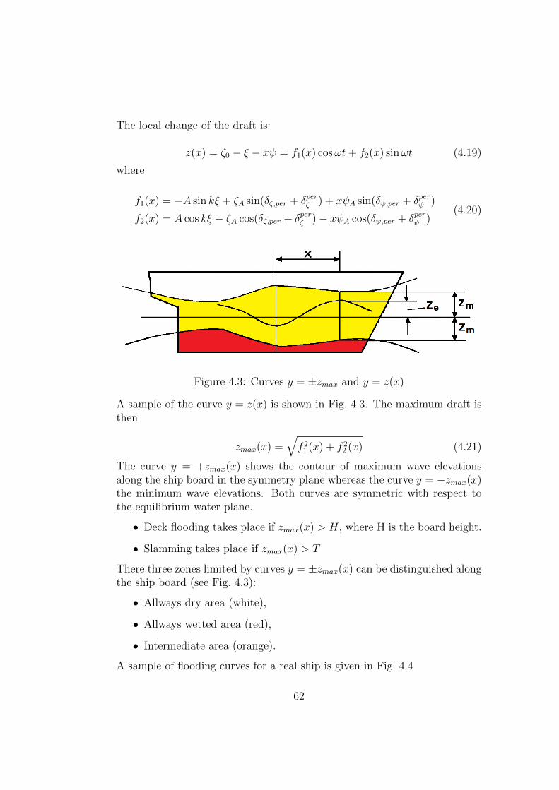
A sample of the curve y = z(x) is shown in Fig. 4.3. The maximum draft isthen
zmax(x) =√f 2
1 (x) + f 22 (x) (4.21)
The curve y = +zmax(x) shows the contour of maximum wave elevationsalong the ship board in the symmetry plane whereas the curve y = −zmax(x)the minimum wave elevations. Both curves are symmetric with respect tothe equilibrium water plane.
• Deck flooding takes place if zmax(x) > H, where H is the board height.
• Slamming takes place if zmax(x) > T
There three zones limited by curves y = ±zmax(x) can be distinguished alongthe ship board (see Fig. 4.3):
• Allways dry area (white),
• Allways wetted area (red),
• Intermediate area (orange).
A sample of flooding curves for a real ship is given in Fig. 4.4
62
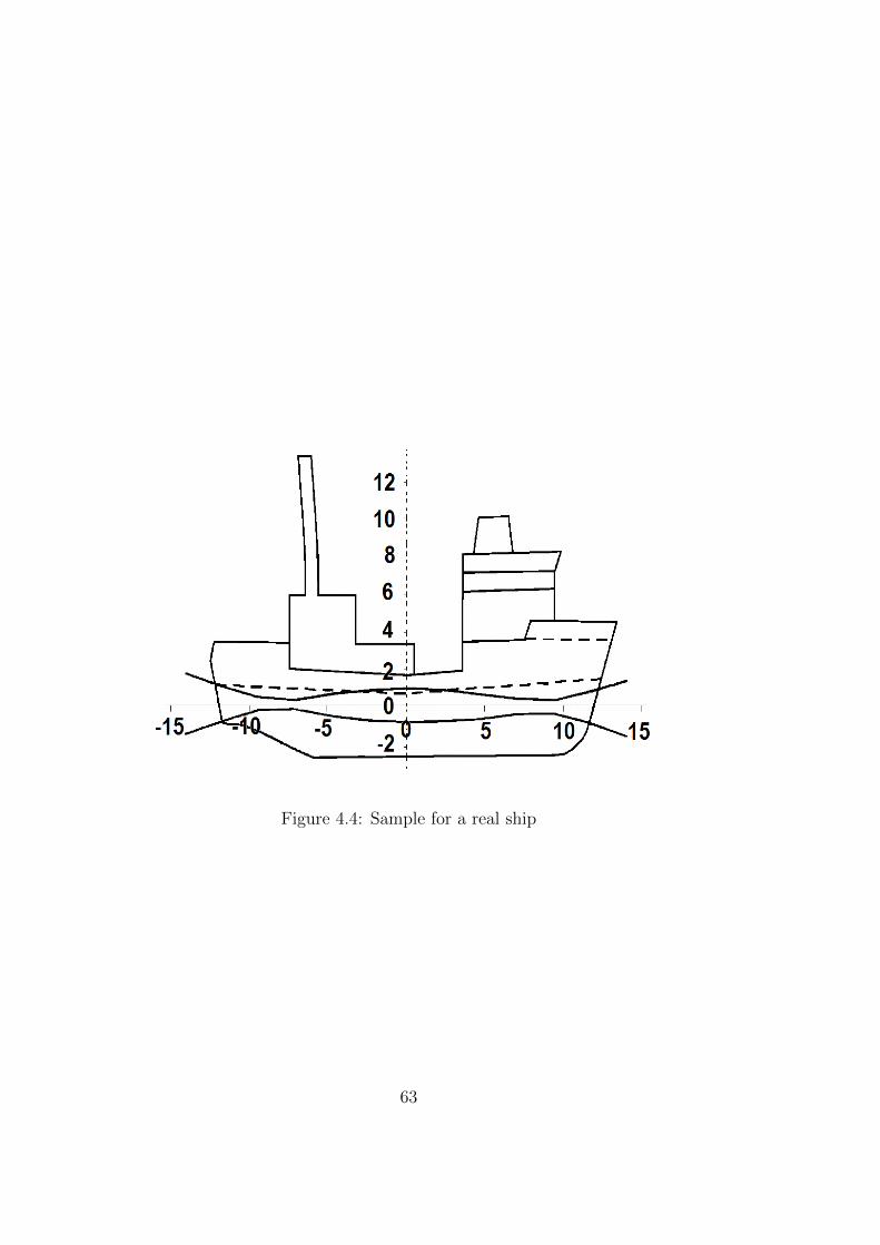
Figure 4.4: Sample for a real ship
63

64
Chapter 5
Seasickness caused by shiposcillations
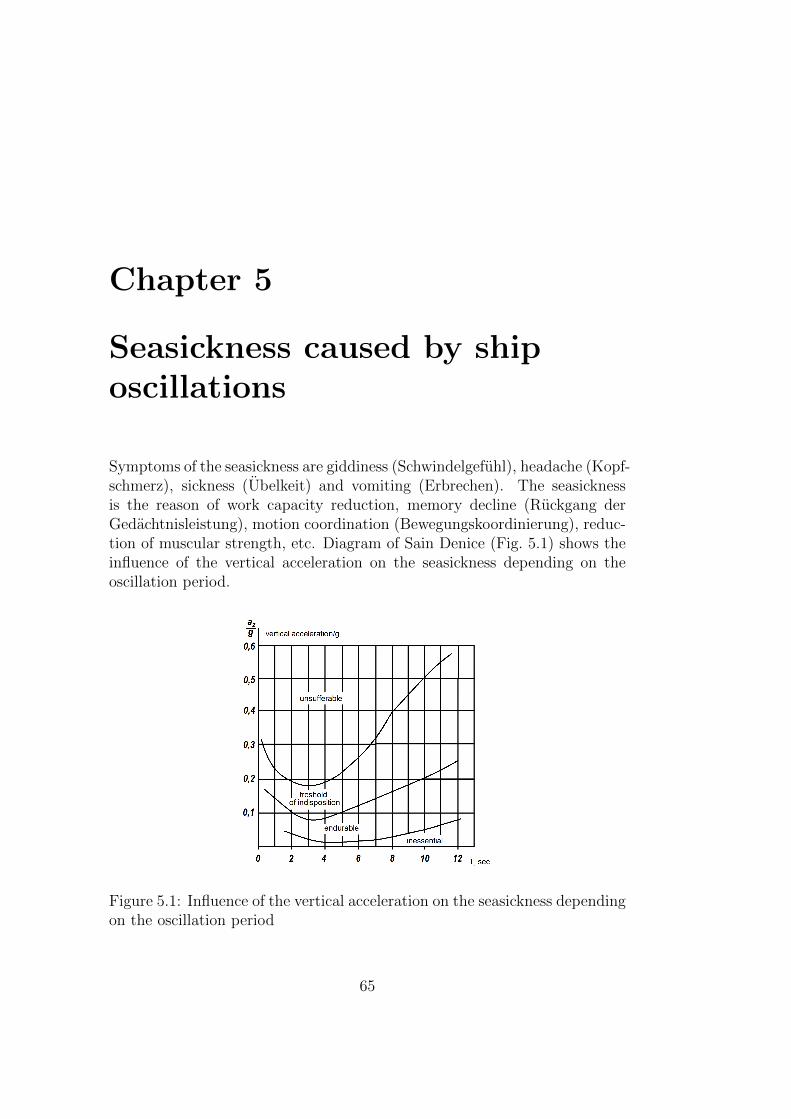
Symptoms of the seasickness are giddiness (Schwindelgefuhl), headache (Kopf-schmerz), sickness (Ubelkeit) and vomiting (Erbrechen). The seasicknessis the reason of work capacity reduction, memory decline (Ruckgang derGedachtnisleistung), motion coordination (Bewegungskoordinierung), reduc-tion of muscular strength, etc. Diagram of Sain Denice (Fig. 5.1) shows theinfluence of the vertical acceleration on the seasickness depending on theoscillation period.
Figure 5.1: Influence of the vertical acceleration on the seasickness dependingon the oscillation period
65
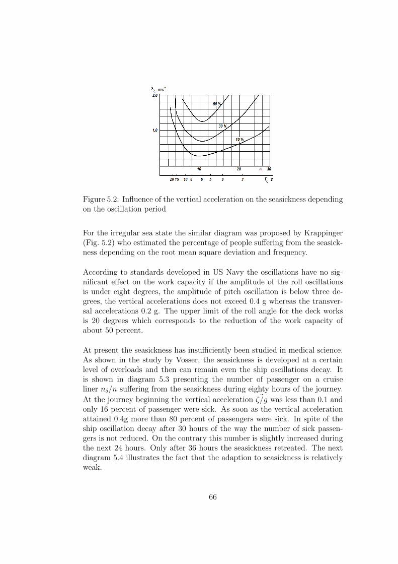
Figure 5.2: Influence of the vertical acceleration on the seasickness dependingon the oscillation period
For the irregular sea state the similar diagram was proposed by Krappinger(Fig. 5.2) who estimated the percentage of people suffering from the seasick-ness depending on the root mean square deviation and frequency.
According to standards developed in US Navy the oscillations have no sig-nificant effect on the work capacity if the amplitude of the roll oscillationsis under eight degrees, the amplitude of pitch oscillation is below three de-grees, the vertical accelerations does not exceed 0.4 g whereas the transver-sal accelerations 0.2 g. The upper limit of the roll angle for the deck worksis 20 degrees which corresponds to the reduction of the work capacity ofabout 50 percent.
At present the seasickness has insufficiently been studied in medical science.As shown in the study by Vosser, the seasickness is developed at a certainlevel of overloads and then can remain even the ship oscillations decay. Itis shown in diagram 5.3 presenting the number of passenger on a cruiseliner nδ/n suffering from the seasickness during eighty hours of the journey.
At the journey beginning the vertical acceleration ¨ζ/g was less than 0.1 andonly 16 percent of passenger were sick. As soon as the vertical accelerationattained 0.4g more than 80 percent of passengers were sick. In spite of theship oscillation decay after 30 hours of the way the number of sick passen-gers is not reduced. On the contrary this number is slightly increased duringthe next 24 hours. Only after 36 hours the seasickness retreated. The nextdiagram 5.4 illustrates the fact that the adaption to seasickness is relativelyweak.
66
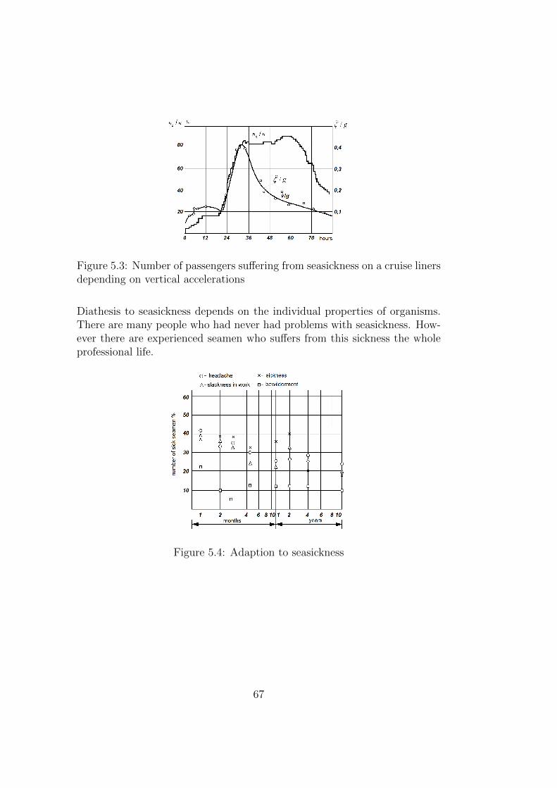
Figure 5.3: Number of passengers suffering from seasickness on a cruise linersdepending on vertical accelerations
Diathesis to seasickness depends on the individual properties of organisms.There are many people who had never had problems with seasickness. How-ever there are experienced seamen who suffers from this sickness the wholeprofessional life.
Figure 5.4: Adaption to seasickness
67

68
Chapter 6
Ship oscillations in irregularwaves
6.1 Representation of irregular waves
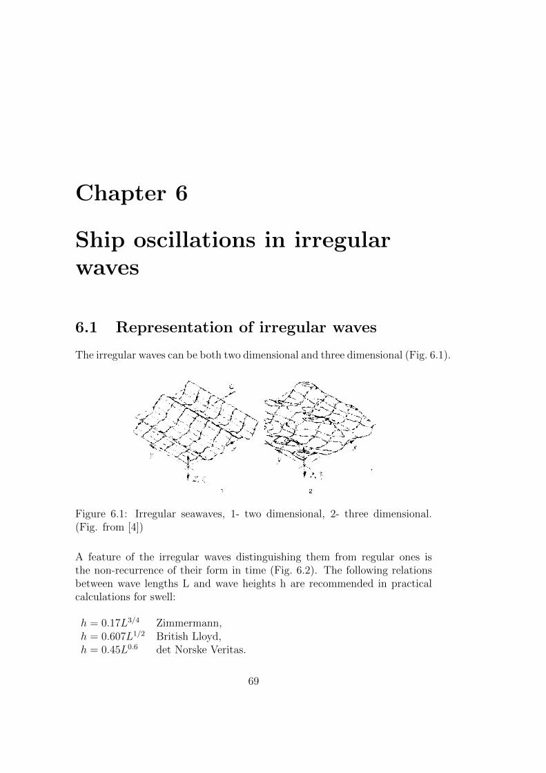
The irregular waves can be both two dimensional and three dimensional (Fig. 6.1).
Figure 6.1: Irregular seawaves, 1- two dimensional, 2- three dimensional.(Fig. from [4])
A feature of the irregular waves distinguishing them from regular ones isthe non-recurrence of their form in time (Fig. 6.2). The following relationsbetween wave lengths L and wave heights h are recommended in practicalcalculations for swell:
h = 0.17L3/4 Zimmermann,h = 0.607L1/2 British Lloyd,h = 0.45L0.6 det Norske Veritas.
69
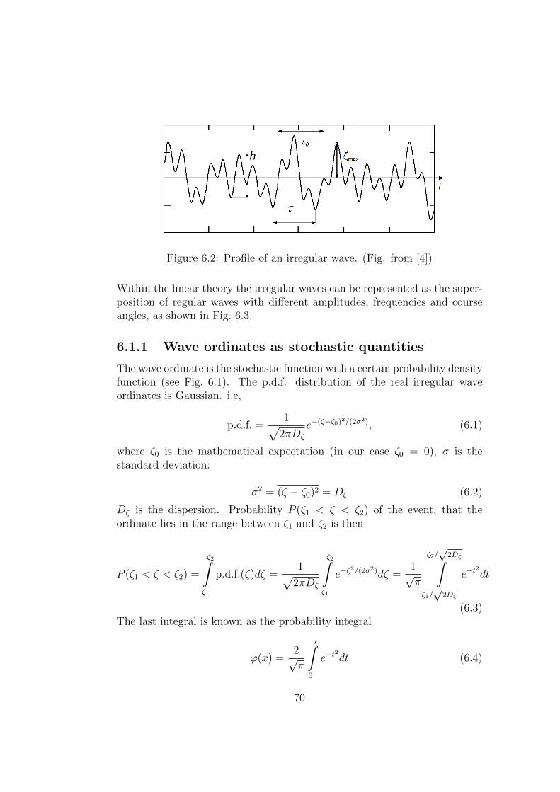
Figure 6.2: Profile of an irregular wave. (Fig. from [4])
Within the linear theory the irregular waves can be represented as the super-position of regular waves with different amplitudes, frequencies and courseangles, as shown in Fig. 6.3.
6.1.1 Wave ordinates as stochastic quantities
The wave ordinate is the stochastic function with a certain probability densityfunction (see Fig. 6.1). The p.d.f. distribution of the real irregular waveordinates is Gaussian. i.e,
p.d.f. =1√
2πDζ
e−(ζ−ζ0)2/(2σ2), (6.1)
where ζ0 is the mathematical expectation (in our case ζ0 = 0), σ is thestandard deviation:
σ2 = (ζ − ζ0)2 = Dζ (6.2)
Dζ is the dispersion. Probability P (ζ1 < ζ < ζ2) of the event, that theordinate lies in the range between ζ1 and ζ2 is then
P (ζ1 < ζ < ζ2) =
ζ2∫ζ1
p.d.f.(ζ)dζ =1√
2πDζ
ζ2∫ζ1
e−ζ2/(2σ2)dζ =
1√π
ζ2/√
2Dζ∫ζ1/√
2Dζ
e−t2
dt
(6.3)The last integral is known as the probability integral
ϕ(x) =2√π
x∫0
e−t2
dt (6.4)
70
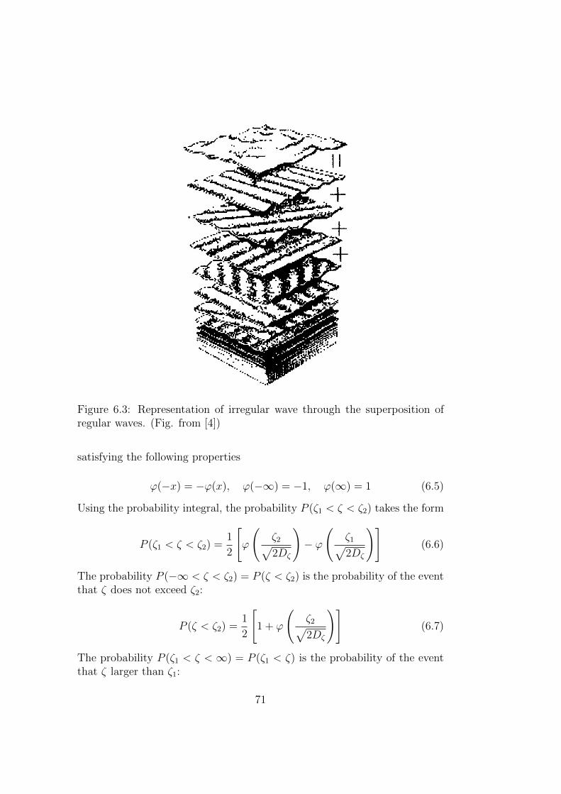
Figure 6.3: Representation of irregular wave through the superposition ofregular waves. (Fig. from [4])
satisfying the following properties
ϕ(−x) = −ϕ(x), ϕ(−∞) = −1, ϕ(∞) = 1 (6.5)
Using the probability integral, the probability P (ζ1 < ζ < ζ2) takes the form
P (ζ1 < ζ < ζ2) =1
2
[ϕ
(ζ2√2Dζ
)− ϕ
(ζ1√2Dζ
)](6.6)
The probability P (−∞ < ζ < ζ2) = P (ζ < ζ2) is the probability of the eventthat ζ does not exceed ζ2:
P (ζ < ζ2) =1
2
[1 + ϕ
(ζ2√2Dζ
)](6.7)
The probability P (ζ1 < ζ < ∞) = P (ζ1 < ζ) is the probability of the eventthat ζ larger than ζ1:
71
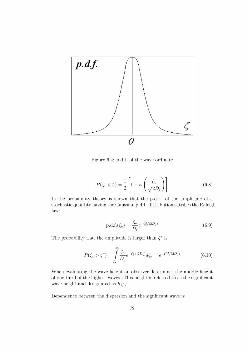
Figure 6.4: p.d.f. of the wave ordinate
P (ζ1 < ζ) =1
2
[1− ϕ
(ζ1√2Dζ
)](6.8)
In the probability theory is shown that the p.d.f. of the amplitude of astochastic quantity having the Gaussian p.d.f. distribution satisfies the Raleighlaw:
p.d.f.(ζa) =ζaDζ
e−ζ2a/(2Dζ) (6.9)
The probability that the amplitude is larger than ζ∗ is
P (ζa > ζ∗) =
∞∫ζ∗
ζaDζ
e−ζ2a/(2Dζ)dζa = e−ζ
∗2/(2Dζ) (6.10)
When evaluating the wave height an observer determines the middle heightof one third of the highest waves. This height is referred to as the significantwave height and designated as h1/3.
Dependence between the dispersion and the significant wave is
72
Dζ = 0.063h21/3 (6.11)
6.1.2 Wave spectra
Irregular waves are considered as the superposition of infinite number ofregular waves of different frequencies, amplitudes and course angles (Fig. 6.3).According to this concept the wave elevation ζ(x, y, t) is represented in formof Fourier - Stieltjes integral:
ζ(x, y, t) = Real
∫∫dA(ω, χ)exp[−ik(x cosχ+ y sinχ) + iωt+ δ(ω, χ)]
(6.12)Here ω is the wave frequency, k is the wave number k = ω2/g, χ is thewave course angle and δ(ω, χ) is the phase angle. The quantity dA(ω, χ, t) isthe function of the amplitude corresponding to the wave propagating at thecourse angle χ < χ < χ + ∆χ with the frequency ω < ω < ω + ∆ω. Themean square elevation is obtained from time averaging the quadrat of theelevation:
ζ2(x, y) = limT→∞1
T
T∫0
ζ2(x, y, t)dt =
=
∫∫dA(ω, χ)exp[−ik(x cosχ+ y sinχ) + iωt+ δ(ω, χ)]
∫∫dA∗(ω1, χ1)exp [−
−ik1(x cosχ1 + y sinχ1)− iω1t− δ(ω, χ)] =1
2
∫∫dA(ω, χ)dA∗(ω, χ)
(6.13)
Here the superscript ∗ stands for the complex conjugate amplitude function.Rigorous derivation of the formula (6.13) can be found in [10]. Multiply-ing ζ2(x, y) with ρg
ρgζ2(x, y) =ρg
2
∫∫dA(ω, χ)dA∗(ω, χ) (6.14)
and comparing the result with the expression for the energy (6.34) derivedin [7]
E = TFl + Ep =ρgA2
2L× 1m
73
One can conclude that ρgζ2(x, y) is the time averaged energy per surfaceunit. Using the representation of the integral
∫∫dA(ω, χ)dA∗(ω, χ) = 2
2π∫0
∞∫0
Sζ(ω, χ)dωdχ (6.15)
we introduce the spectral density of the irregular waves Sζ(ω, χ) which isthe contribution of the wave with the frequency ω < ω < ω + ∆ω and thecourse angle χ < χ < χ + ∆χ to the irregular wave energy. Commonly thefunction Sζ(ω, χ) is called shortly the wave spectrum.
At present there is no much information on the energy distribution both onthe frequency and the course angle. The typical measurements with buoydo not provide information about the dependency of wave elevations on thecourse angle. In the ship theory is assumed that the irregular waves have apreferential propagation direction and the wave have long wave crest. Thewaves are approximately two dimensional. Such rough sea can fully be char-acterized by the frequency spectrum Sζ(ω) defining as
Sζ(ω) =
2π∫0
Sζ(ω, χ)dχ (6.16)
The spectrum of the wave state Sζ(ω) shows the distribution of the wave en-ergy on frequencies. The two dimensional spectrum Sζ(ω, χ) can be restoredfrom the one dimensional one Sζ(ω) using the following simple approxima-tion:
Sζ(ω, χ) =4
3πSζ(ω) cos4 χ
To determine the spectrum, the wave ordinates are measured and representedin Fourier series. The energy ∆E(ω < ω < ω + ∆ω) is calculated as thesquared wave ordinate for each interval of the frequencies ∆ω. The spectraldensity of waves is calculated as
Sζ(ω) = lim∆ω→0
∆E(ω < ω < ω + ∆ω)
∆ω(6.17)
From the probability theory:
Dζ =
∞∫0
Sζ(ω)dω (6.18)
74
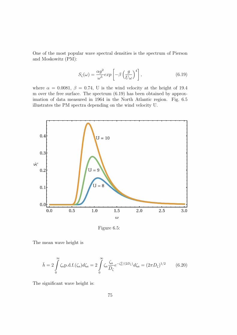
One of the most popular wave spectral densities is the spectrum of Piersonand Moskowitz (PM):
Sζ(ω) =αg2
ω5exp
[−β( g
Uω
)4], (6.19)
where α = 0.0081, β = 0.74, U is the wind velocity at the height of 19.4m over the free surface. The spectrum (6.19) has been obtained by approx-imation of data measured in 1964 in the North Atlantic region. Fig. 6.5illustrates the PM spectra depending on the wind velocity U.
Figure 6.5:
The mean wave height is
h = 2
∞∫0
ζap.d.f.(ζa)dζa = 2
∞∫0
ζaζaDζ
e−ζ2a/(2Dζ)dζa = (2πDζ)
1/2 (6.20)
The significant wave height is:
75
h1/3 =
2∞∫ζ1
ζap.d.f.(ζa)dζa
∞∫ζ1
p.d.f.(ζa)dζa
(6.21)
where the amplitude ζ1 is chosen from the condition
∞∫ζ1
p.d.f.(ζa)dζa = 1/3⇒ e−ζ21/(2Dζ) = 1/3⇒ ζ1 =
√2Dζln3 (6.22)
It follows from (6.9) and (6.21):
h1/3 = 4√Dζ (6.23)
The middle frequency is defined as
ω =
∞∫0
ω2Sζ(ω)dω
∞∫0
Sζ(ω)dω
1/2
=
∞∫0
ω2Sζ(ω)dω
Dζ(ω)
1/2
(6.24)
Substitution of (6.19) into (6.18), (6.23) and (6.24) results in
h1/3 = 2U2
g
[α
β
]1/2
, ω = (πβ)1/4(g/U) (6.25)
6.2 Calculation of ship oscillations in irregu-
lar waves
Using the assumption of small waves we can substitute the superposition ofregular waves into equations (3.20) and (3.21) describing the heave and rolloscillations. Since the equations are linear the responses of the ship to eachregular wave can be calculated separately. In this case one can obtain thehistory of oscillations in time.
However, from point of view of practical applications only the statistical pa-rameters of oscillations are of importance. To determine them, the ship isconsidered as the dynamic system. The seaway is the input which is trans-formed by the ship into oscillations considered as the output. In the statisti-cal theory shown, that if the input signal has the Gaussian p.d.f. distribution
76
the output signal has also the Gaussian p.d.f. distribution. With the otherwords, the ship oscillation parameters (roll angle, etc) obey the normal Gaus-sian law whereas the amplitudes of oscillation parameters satisfy the Raleighlaw. The only unknown value in these distributions laws is the dispersion D.
Let us consider the roll oscillations of a ship with the zero forward speed.As shown in the previous lectures the ratio of the roll oscillations amplitude(output signal) to the wave slope amplitude (input signal) is given by theformula
ϕ(r)A
αA=ϕA − αAαA
=ω2/(1 + kϕ)√
(1− ω2)2 + 4ν2ω2⇒ ϕA
αA=
=ω2/(1 + kϕ)√
(1− ω2)2 + 4ν2ω2+ 1 = Φ(ω)
where
Φ(ω) =ω2/(1 + kϕ)√
(1− ω2)2 + 4ν2ω2+ 1 (6.26)
is the so called response function. Since the wave spectral density is propor-tional to the wave ordinates squared and taking the superposition principleinto account, we obtain the following relation between the spectral densityof the seaway and the spectral density of oscillations
Sϕ(ω) = Φ2(ω)Sζ(ω) (6.27)
or
Sϕ(ω) = Sζ(ω)
[ω2/(1 + kϕ)√
(1− ω2)2 + 4ν2ω2+ 1
]2
(6.28)
Dispersion of the roll oscillations and the standard deviation are found fromthe definitions (6.2) and (6.18)
Dϕ =
∞∫0
Sϕ(ω)dω =
∞∫0
Φ2(ω)Sζ(ω)dω, σϕ =√Dϕ (6.29)
Similar formulae can be obtained for angular roll velocity and acceleration
Dϕ =
∞∫0
ω2Sϕ(ω)dω, σϕ =√Dϕ (6.30)
77
Dϕ =
∞∫0
ω4Sϕ(ω)dω, σϕ =√Dϕ (6.31)
The dispersions obtained from (6.29), (6.30) and (6.31) determine fully theirregular ship oscillations in heavy seaway. Using them the following furtherparameters can be calculated
• Most probable amplitude of oscillations corresponding to the maximumof the p.d.f.(ζa) distribution
ϕm = σϕ (6.32)
The probability that the roll amplitude exceeds ϕm is 60.6 %.
• Averaged amplitude of roll oscillations (mathematical expectation)
ϕ =
√π
2σϕ ≈ 1.25σϕ (6.33)
The probability that the roll amplitude exceeds ϕ is 45.6 %.
• The probability that the roll amplitude exceeds the value ϕ∗:
p(ϕA > ϕ∗) = e−0.5(ϕ∗/σϕ)2 (6.34)
• Averaged frequency and averaged period of oscillations:
ωϕ =σϕσϕ, Tϕ =
2π
ωϕ= 2π
σϕσϕ
(6.35)
• Number of ship inclinations (semi periods) within the time interval t:
Nt =2t
Tϕ(6.36)
• Number of ship inclinations within the time interval t provided the rollangle amplitude is larger than ϕ∗:
Nϕ∗ = NtP (ϕA > ϕ∗) =2t
Tϕe−0.5(ϕ∗/σϕ)2 (6.37)
The formulae (6.32) - 6.37) are derived under assumption that the oscillationsobey the Gaussian and Raleigh distribution law.
78
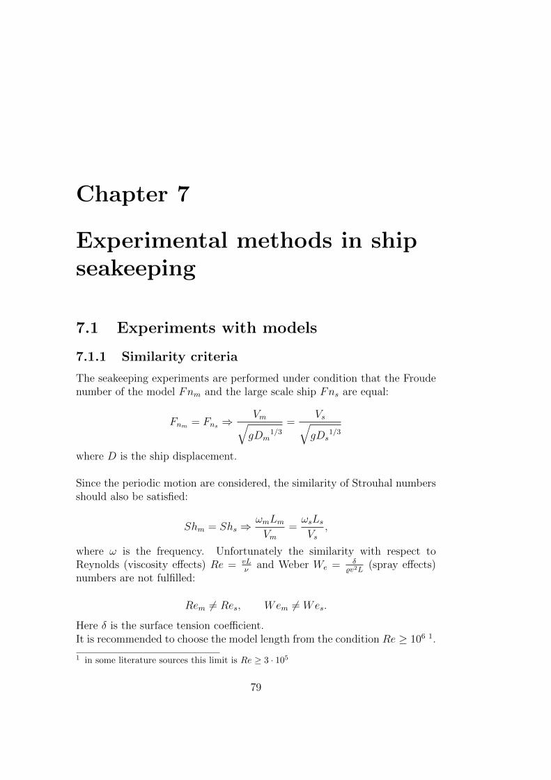
Chapter 7
Experimental methods in shipseakeeping
7.1 Experiments with models
7.1.1 Similarity criteria
The seakeeping experiments are performed under condition that the Froudenumber of the model Fnm and the large scale ship Fns are equal:
Fnm = Fns ⇒Vm√gDm
1/3=
Vs√gDs
1/3
where D is the ship displacement.
Since the periodic motion are considered, the similarity of Strouhal numbersshould also be satisfied:
Shm = Shs ⇒ωmLmVm
=ωsLsVs
,
where ω is the frequency. Unfortunately the similarity with respect toReynolds (viscosity effects) Re = vL
νand Weber We = δ
%v2L(spray effects)
numbers are not fulfilled:
Rem 6= Res, Wem 6= Wes.
Here δ is the surface tension coefficient.It is recommended to choose the model length from the condition Re ≥ 106 1.
1 in some literature sources this limit is Re ≥ 3 · 105
79
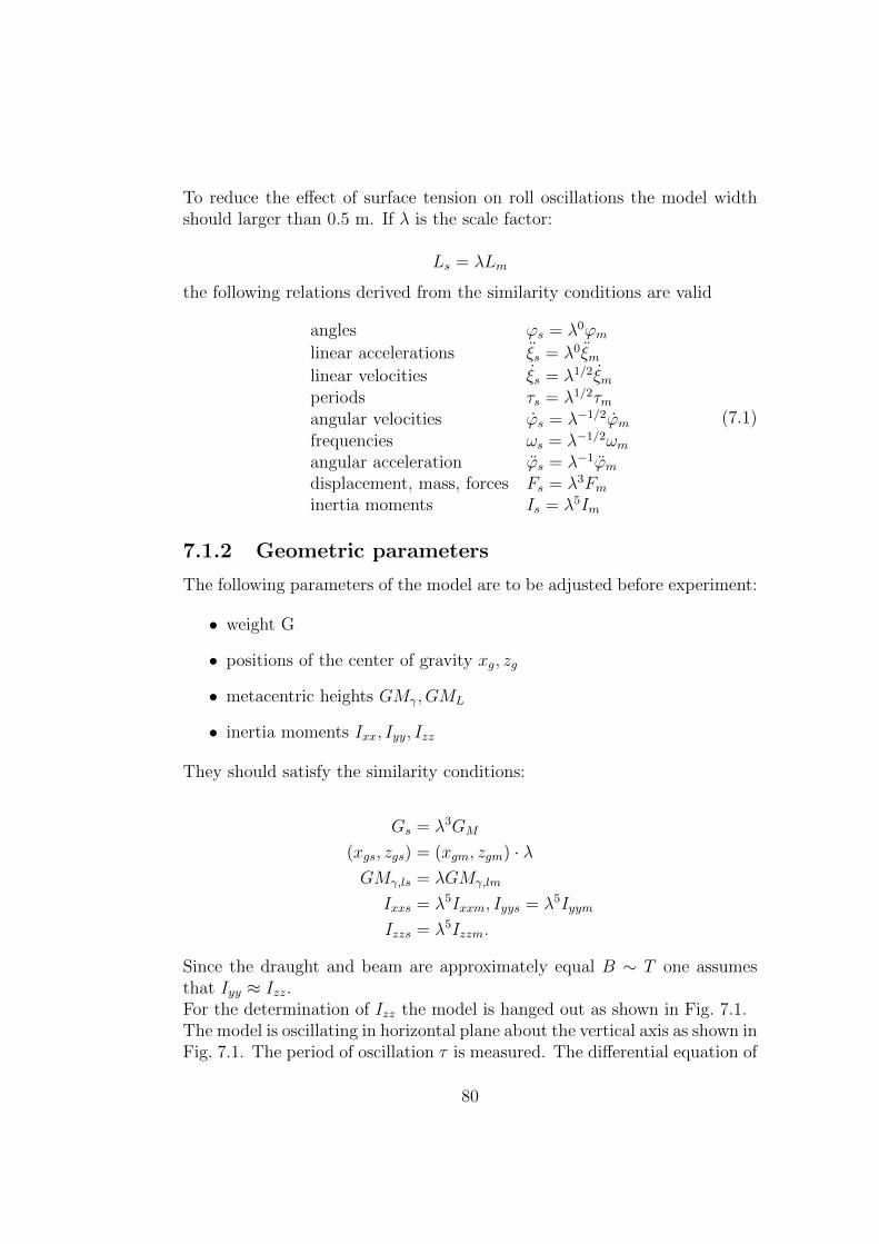
To reduce the effect of surface tension on roll oscillations the model widthshould larger than 0.5 m. If λ is the scale factor:
Ls = λLm
the following relations derived from the similarity conditions are valid
angles ϕs = λ0ϕmlinear accelerations ξs = λ0ξmlinear velocities ξs = λ1/2ξmperiods τs = λ1/2τmangular velocities ϕs = λ−1/2ϕmfrequencies ωs = λ−1/2ωmangular acceleration ϕs = λ−1ϕmdisplacement, mass, forces Fs = λ3Fminertia moments Is = λ5Im
(7.1)
7.1.2 Geometric parameters
The following parameters of the model are to be adjusted before experiment:
• weight G
• positions of the center of gravity xg, zg
• metacentric heights GMγ, GML
• inertia moments Ixx, Iyy, Izz
They should satisfy the similarity conditions:
Gs = λ3GM
(xgs, zgs) = (xgm, zgm) · λGMγ,ls = λGMγ,lm
Ixxs = λ5Ixxm, Iyys = λ5Iyym
Izzs = λ5Izzm.
Since the draught and beam are approximately equal B ∼ T one assumesthat Iyy ≈ Izz.For the determination of Izz the model is hanged out as shown in Fig. 7.1.The model is oscillating in horizontal plane about the vertical axis as shown inFig. 7.1. The period of oscillation τ is measured. The differential equation of
80
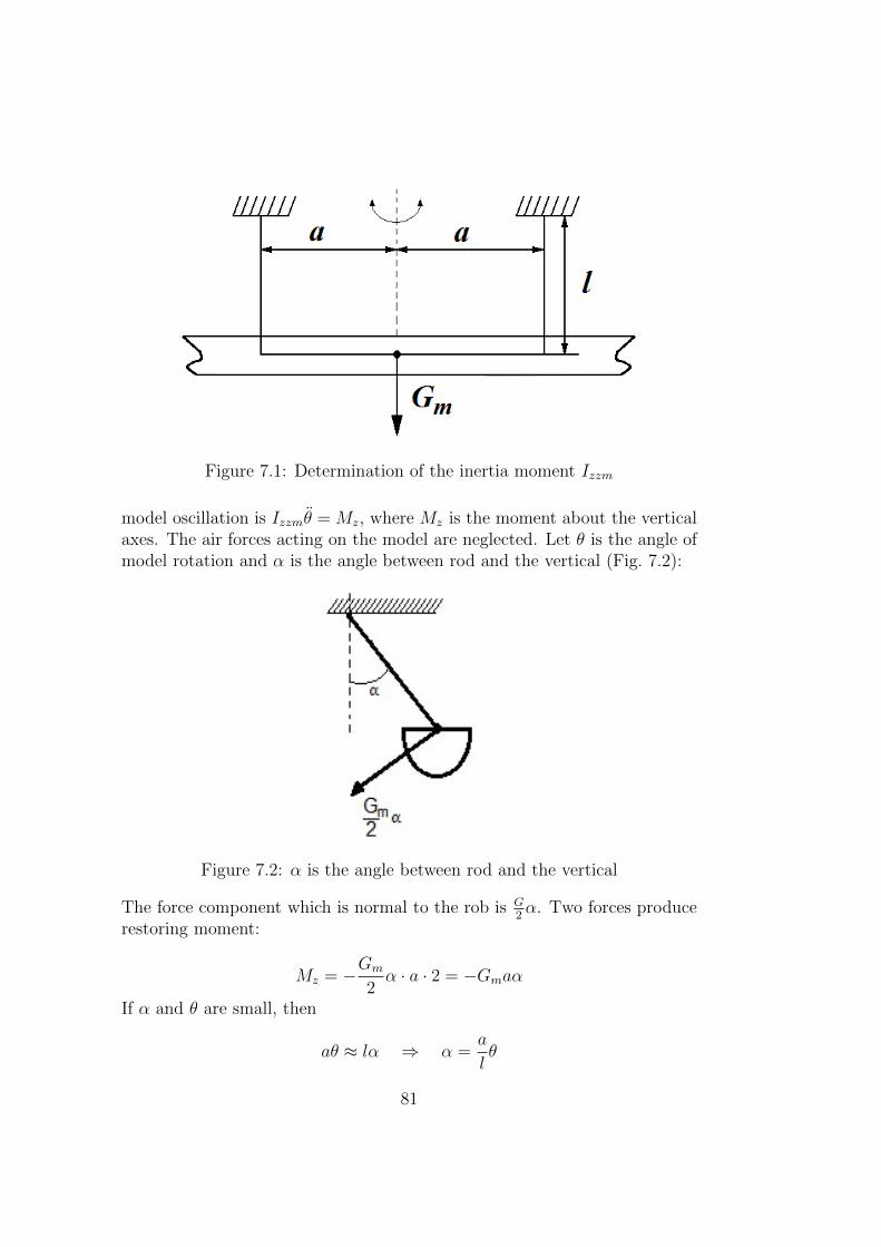
Figure 7.1: Determination of the inertia moment Izzm
model oscillation is Izzmθ = Mz, where Mz is the moment about the verticalaxes. The air forces acting on the model are neglected. Let θ is the angle ofmodel rotation and α is the angle between rod and the vertical (Fig. 7.2):
Figure 7.2: α is the angle between rod and the vertical
The force component which is normal to the rob is G2α. Two forces produce
restoring moment:
Mz = −Gm
2α · a · 2 = −Gmaα
If α and θ are small, then
aθ ≈ lα ⇒ α =a
lθ
81
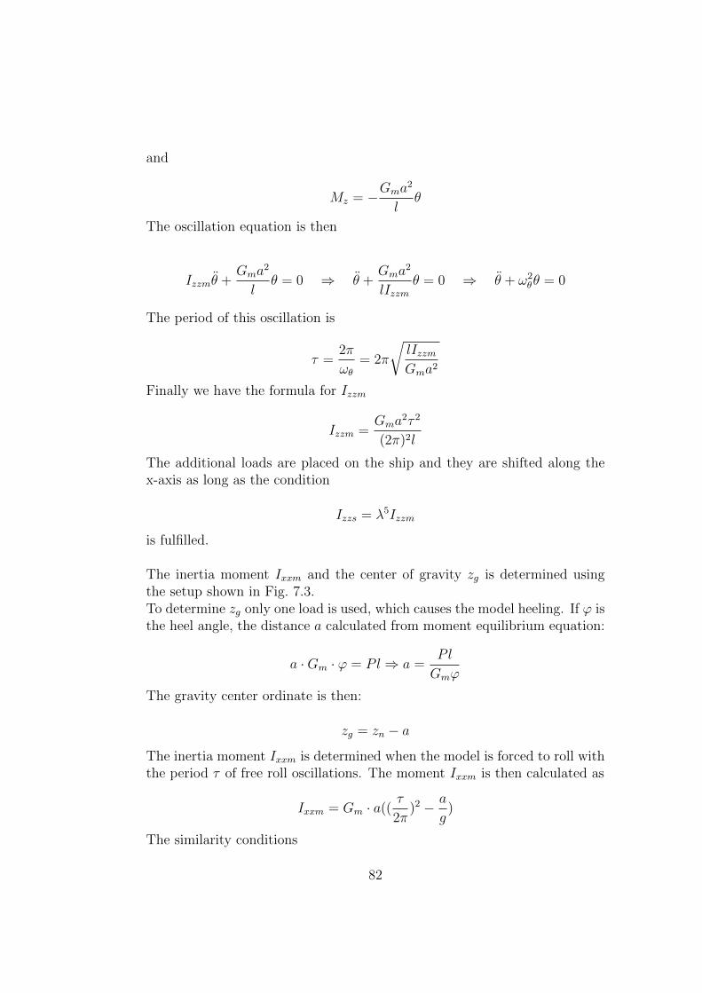
and
Mz = −Gma2
lθ
The oscillation equation is then
Izzmθ +Gma
2
lθ = 0 ⇒ θ +
Gma2
lIzzmθ = 0 ⇒ θ + ω2
θθ = 0
The period of this oscillation is
τ =2π
ωθ= 2π
√lIzzmGma2
Finally we have the formula for Izzm
Izzm =Gma
2τ 2
(2π)2l
The additional loads are placed on the ship and they are shifted along thex-axis as long as the condition
Izzs = λ5Izzm
is fulfilled.
The inertia moment Ixxm and the center of gravity zg is determined usingthe setup shown in Fig. 7.3.To determine zg only one load is used, which causes the model heeling. If ϕ isthe heel angle, the distance a calculated from moment equilibrium equation:
a ·Gm · ϕ = Pl⇒ a =Pl
Gmϕ
The gravity center ordinate is then:
zg = zn − a
The inertia moment Ixxm is determined when the model is forced to roll withthe period τ of free roll oscillations. The moment Ixxm is then calculated as
Ixxm = Gm · a((τ
2π)2 − a
g)
The similarity conditions
82
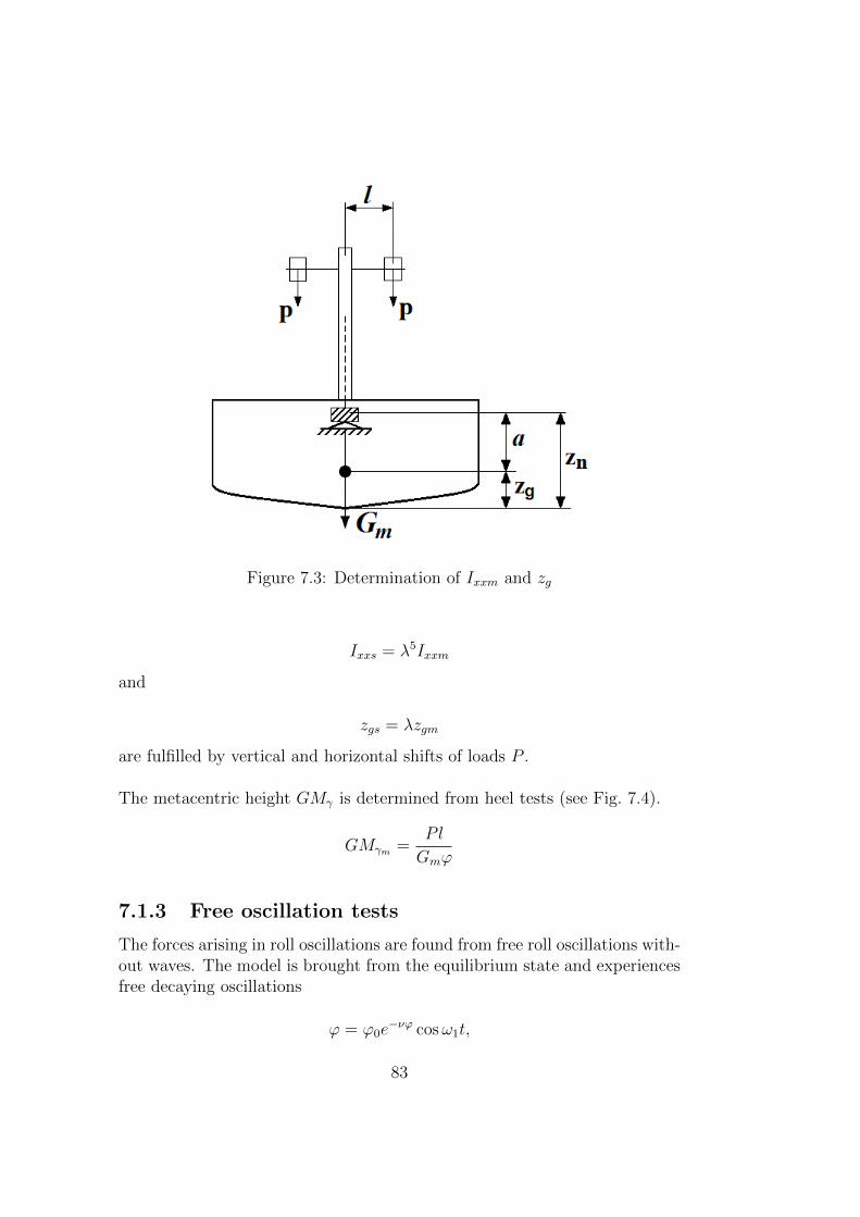
Figure 7.3: Determination of Ixxm and zg
Ixxs = λ5Ixxm
and
zgs = λzgm
are fulfilled by vertical and horizontal shifts of loads P .
The metacentric height GMγ is determined from heel tests (see Fig. 7.4).
GMγm =Pl
Gmϕ
7.1.3 Free oscillation tests
The forces arising in roll oscillations are found from free roll oscillations with-out waves. The model is brought from the equilibrium state and experiencesfree decaying oscillations
ϕ = ϕ0e−νϕ cosω1t,
83
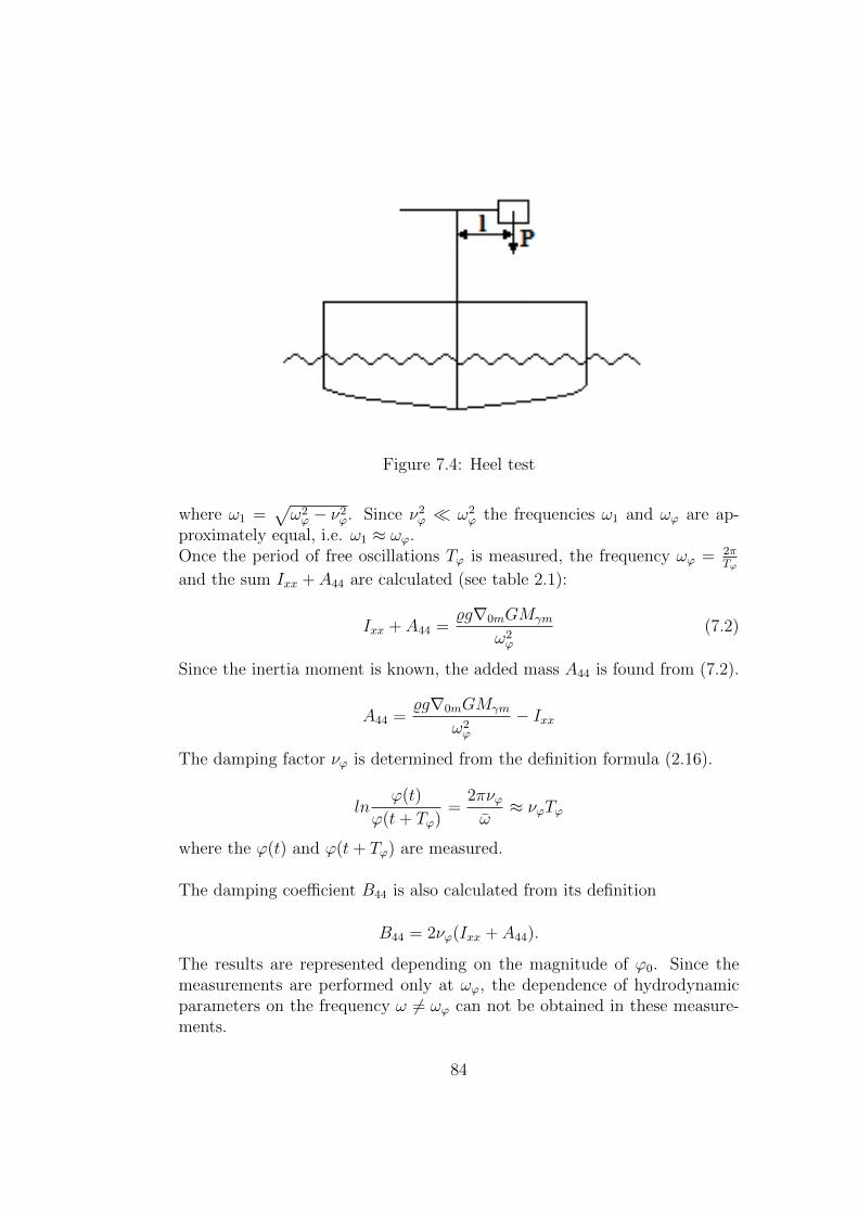
Figure 7.4: Heel test
where ω1 =√ω2ϕ − ν2
ϕ. Since ν2ϕ � ω2
ϕ the frequencies ω1 and ωϕ are ap-proximately equal, i.e. ω1 ≈ ωϕ.Once the period of free oscillations Tϕ is measured, the frequency ωϕ = 2π
Tϕ
and the sum Ixx + A44 are calculated (see table 2.1):
Ixx + A44 =%g∇0mGMγm
ω2ϕ
(7.2)
Since the inertia moment is known, the added mass A44 is found from (7.2).
A44 =%g∇0mGMγm
ω2ϕ
− Ixx
The damping factor νϕ is determined from the definition formula (2.16).
lnϕ(t)
ϕ(t+ Tϕ)=
2πνϕω≈ νϕTϕ
where the ϕ(t) and ϕ(t+ Tϕ) are measured.
The damping coefficient B44 is also calculated from its definition
B44 = 2νϕ(Ixx + A44).
The results are represented depending on the magnitude of ϕ0. Since themeasurements are performed only at ωϕ, the dependence of hydrodynamicparameters on the frequency ω 6= ωϕ can not be obtained in these measure-ments.
84
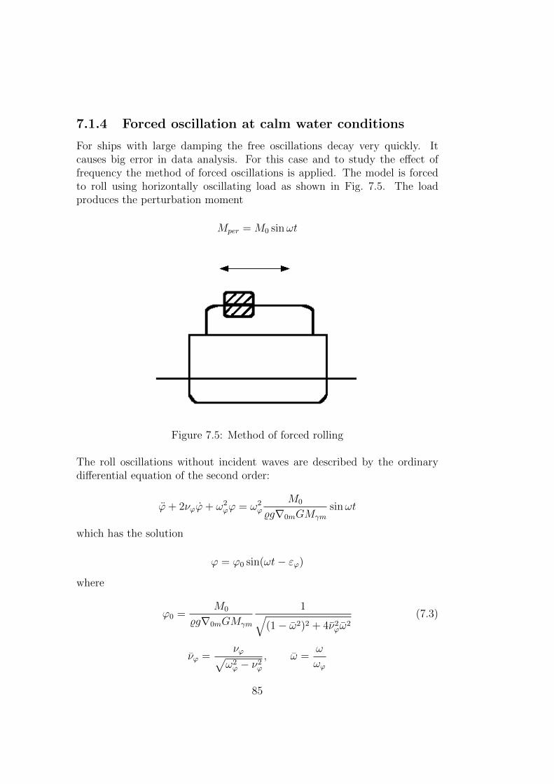
7.1.4 Forced oscillation at calm water conditions
For ships with large damping the free oscillations decay very quickly. Itcauses big error in data analysis. For this case and to study the effect offrequency the method of forced oscillations is applied. The model is forcedto roll using horizontally oscillating load as shown in Fig. 7.5. The loadproduces the perturbation moment
Mper = M0 sinωt
Figure 7.5: Method of forced rolling
The roll oscillations without incident waves are described by the ordinarydifferential equation of the second order:
ϕ+ 2νϕϕ+ ω2ϕϕ = ω2
ϕ
M0
%g∇0mGMγm
sinωt
which has the solution
ϕ = ϕ0 sin(ωt− εϕ)
where
ϕ0 =M0
%g∇0mGMγm
1√(1− ω2)2 + 4ν2
ϕω2
(7.3)
νϕ =νϕ√
ω2ϕ − ν2
ϕ
, ω =ω
ωϕ
85
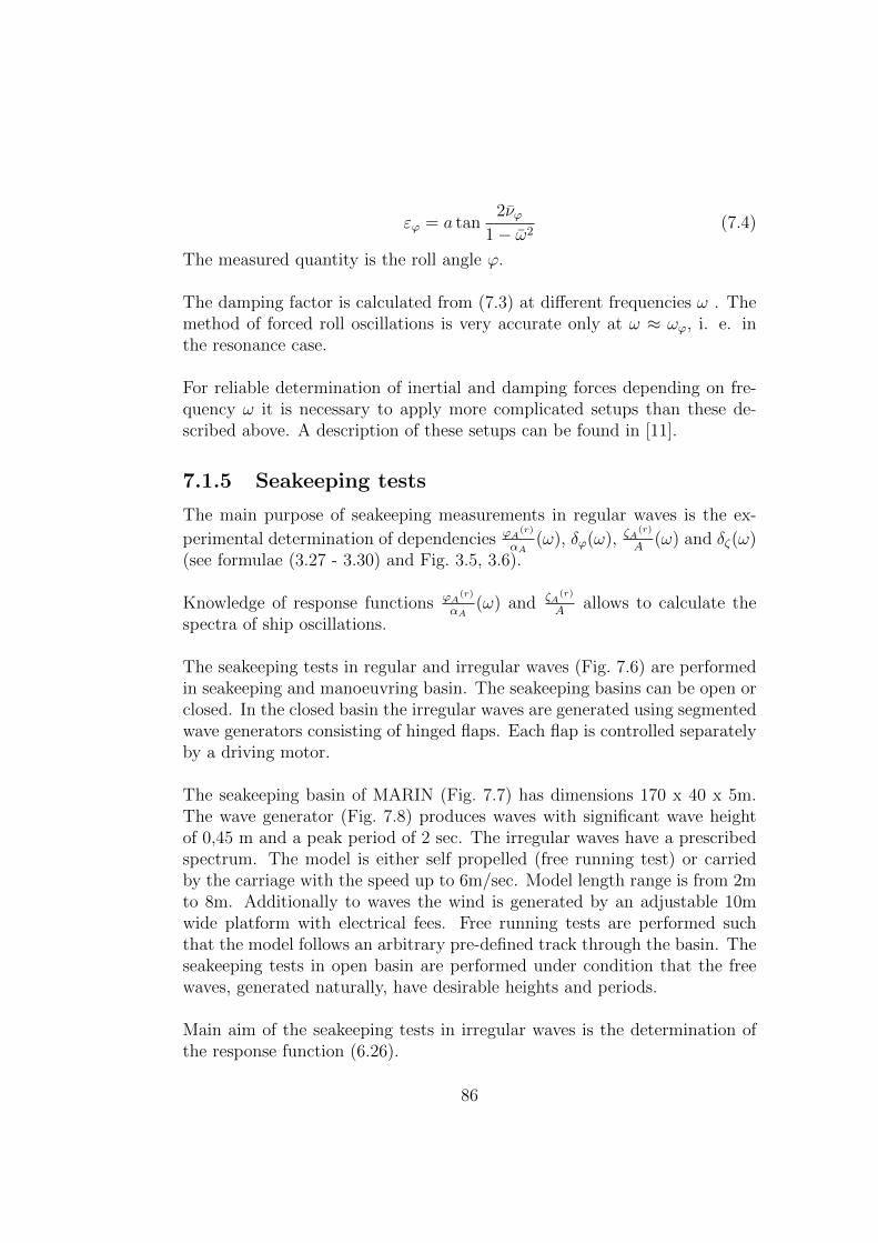
εϕ = a tan2νϕ
1− ω2(7.4)
The measured quantity is the roll angle ϕ.
The damping factor is calculated from (7.3) at different frequencies ω . Themethod of forced roll oscillations is very accurate only at ω ≈ ωϕ, i. e. inthe resonance case.
For reliable determination of inertial and damping forces depending on fre-quency ω it is necessary to apply more complicated setups than these de-scribed above. A description of these setups can be found in [11].
7.1.5 Seakeeping tests
The main purpose of seakeeping measurements in regular waves is the ex-
perimental determination of dependencies ϕA(r)
αA(ω), δϕ(ω), ζA
(r)
A(ω) and δζ(ω)
(see formulae (3.27 - 3.30) and Fig. 3.5, 3.6).
Knowledge of response functions ϕA(r)
αA(ω) and ζA
(r)
Aallows to calculate the
spectra of ship oscillations.
The seakeeping tests in regular and irregular waves (Fig. 7.6) are performedin seakeeping and manoeuvring basin. The seakeeping basins can be open orclosed. In the closed basin the irregular waves are generated using segmentedwave generators consisting of hinged flaps. Each flap is controlled separatelyby a driving motor.
The seakeeping basin of MARIN (Fig. 7.7) has dimensions 170 x 40 x 5m.The wave generator (Fig. 7.8) produces waves with significant wave heightof 0,45 m and a peak period of 2 sec. The irregular waves have a prescribedspectrum. The model is either self propelled (free running test) or carriedby the carriage with the speed up to 6m/sec. Model length range is from 2mto 8m. Additionally to waves the wind is generated by an adjustable 10mwide platform with electrical fees. Free running tests are performed suchthat the model follows an arbitrary pre-defined track through the basin. Theseakeeping tests in open basin are performed under condition that the freewaves, generated naturally, have desirable heights and periods.
Main aim of the seakeeping tests in irregular waves is the determination ofthe response function (6.26).
86
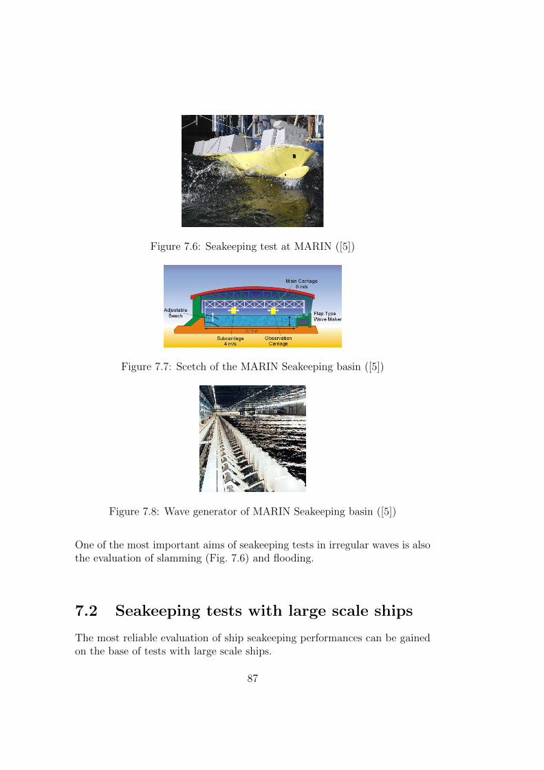
Figure 7.6: Seakeeping test at MARIN ([5])
Figure 7.7: Scetch of the MARIN Seakeeping basin ([5])
Figure 7.8: Wave generator of MARIN Seakeeping basin ([5])
One of the most important aims of seakeeping tests in irregular waves is alsothe evaluation of slamming (Fig. 7.6) and flooding.
7.2 Seakeeping tests with large scale ships
The most reliable evaluation of ship seakeeping performances can be gainedon the base of tests with large scale ships.
87
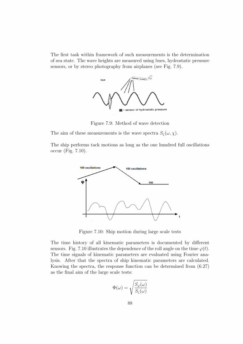
The first task within framework of such measurements is the determinationof sea state. The wave heights are measured using bues, hydrostatic pressuresensors, or by stereo photography from airplanes (see Fig. 7.9).
Figure 7.9: Method of wave detection
The aim of these measurements is the wave spectra Sζ(ω, χ).
The ship performs tack motions as long as the one hundred full oscillationsoccur (Fig. 7.10).
Figure 7.10: Ship motion during large scale tests
The time history of all kinematic parameters is documented by differentsensors. Fig. 7.10 illustrates the dependence of the roll angle on the time ϕ(t).The time signals of kinematic parameters are evaluated using Fourier ana-lysis. After that the spectra of ship kinematic parameters are calculated.Knowing the spectra, the response function can be determined from (6.27)as the final aim of the large scale tests:
Φ(ω) =
√Sϕ(ω)
Sζ(ω)
88
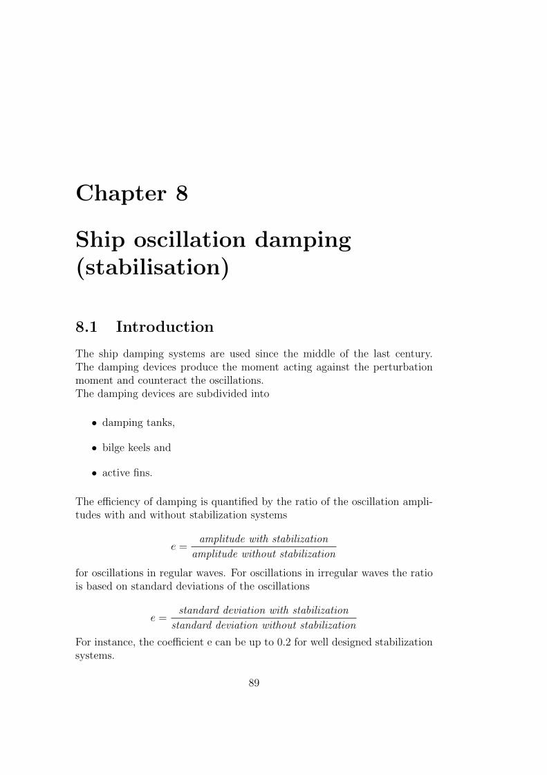
Chapter 8
Ship oscillation damping(stabilisation)
8.1 Introduction
The ship damping systems are used since the middle of the last century.The damping devices produce the moment acting against the perturbationmoment and counteract the oscillations.The damping devices are subdivided into
• damping tanks,
• bilge keels and
• active fins.
The efficiency of damping is quantified by the ratio of the oscillation ampli-tudes with and without stabilization systems
e =amplitude with stabilization
amplitude without stabilization
for oscillations in regular waves. For oscillations in irregular waves the ratiois based on standard deviations of the oscillations
e =standard deviation with stabilization
standard deviation without stabilization
For instance, the coefficient e can be up to 0.2 for well designed stabilizationsystems.
89
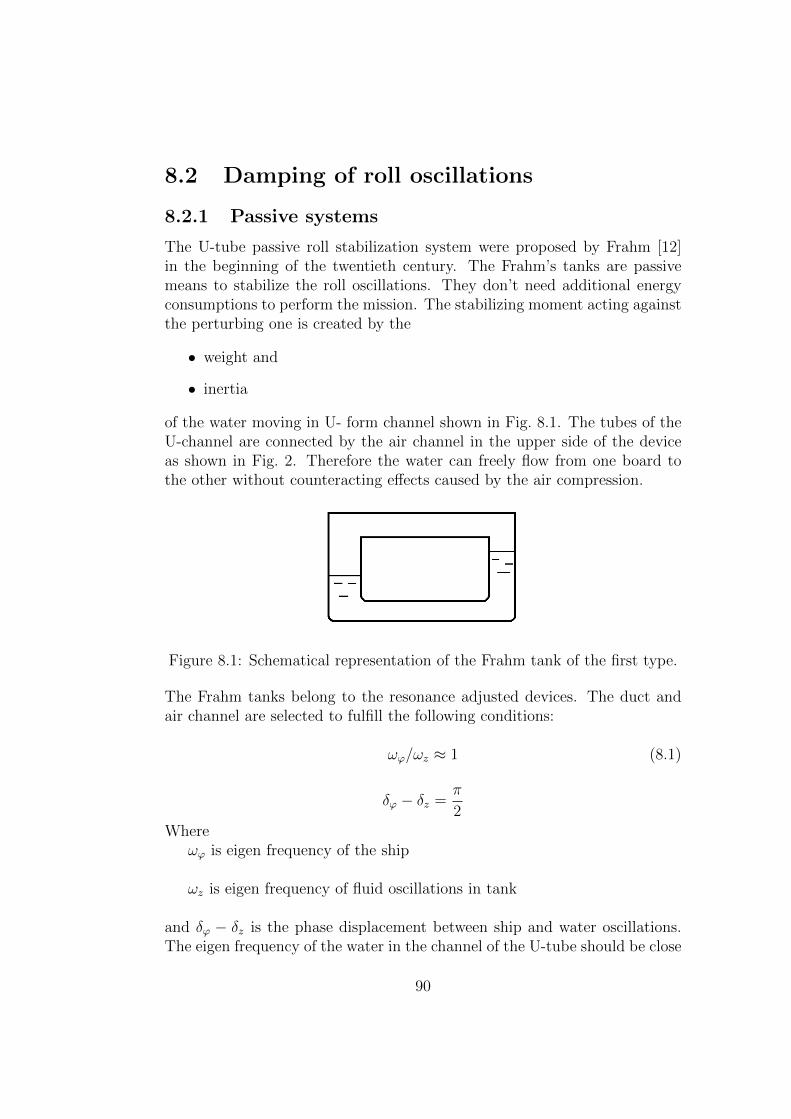
8.2 Damping of roll oscillations
8.2.1 Passive systems
The U-tube passive roll stabilization system were proposed by Frahm [12]in the beginning of the twentieth century. The Frahm’s tanks are passivemeans to stabilize the roll oscillations. They don’t need additional energyconsumptions to perform the mission. The stabilizing moment acting againstthe perturbing one is created by the
• weight and
• inertia
of the water moving in U- form channel shown in Fig. 8.1. The tubes of theU-channel are connected by the air channel in the upper side of the deviceas shown in Fig. 2. Therefore the water can freely flow from one board tothe other without counteracting effects caused by the air compression.
Figure 8.1: Schematical representation of the Frahm tank of the first type.
The Frahm tanks belong to the resonance adjusted devices. The duct andair channel are selected to fulfill the following conditions:
ωϕ/ωz ≈ 1 (8.1)
δϕ − δz =π
2Where
ωϕ is eigen frequency of the ship
ωz is eigen frequency of fluid oscillations in tank
and δϕ − δz is the phase displacement between ship and water oscillations.The eigen frequency of the water in the channel of the U-tube should be close
90
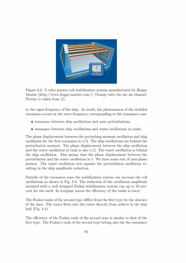
Figure 8.2: U-tube passive roll stabilization system manufactured by HoppeMarine (http://www.hoppe-marine.com/). Orange tube the are air channel.Picture is taken from [1].
to the eigen frequency of the ship. As result, the phenomenon of the doubledresonance occurs at the wave frequency corresponding to the resonance case:
• resonance between ship oscillations and wave perturbations,
• resonance between ship oscillations and water oscillations in tanks.
The phase displacement between the perturbing moment oscillation and shiposcillation for the first resonance is π/2. The ship oscillations are behind theperturbation moment. The phase displacement between the ship oscillationand the water oscillation in tank is also π/2. The water oscillation is behindthe ship oscillation. This means that the phase displacement between theperturbation and the water oscillation is π. We have some sort of anti-phasemotion. The water oscillation acts against the perturbation oscillation re-sulting in the ship amplitude reduction.
Outside of the resonance zone the stabilization system can increase the rolloscillations as shown in Fig. 8.3. The reduction of the oscillation amplitudeattained with a well designed Frahm stabilization system can up to 50 per-cent for the swell. In irregular waves the efficiency of the tanks is lower.
The Frahm tanks of the second type differs from the first type by the absenceof the duct. The water flows into the tubes directly from orifices in the shiphull (Fig. 8.4).
The efficiency of the Frahm tank of the second type is similar to that of thefirst type. The Frahm’s tank of the second type belong also the the resonance
91
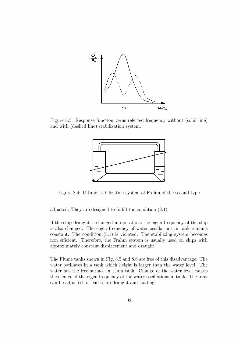
Figure 8.3: Response function verus referred frequency without (solid line)and with (dashed line) stabilization system.
Figure 8.4: U-tube stabilization system of Frahm of the second type
adjusted. They are designed to fulfill the condition (8.1).
If the ship draught is changed in operations the eigen frequency of the shipis also changed. The eigen frequency of water oscillations in tank remainsconstant. The condition (8.1) is violated. The stabilizing system becomesnon efficient. Therefore, the Frahm system is usually used on ships withapproximately constant displacement and draught.
The Flume tanks shown in Fig. 8.5 and 8.6 are free of this disadvantage. Thewater oscillates in a tank which height is larger than the water level. Thewater has the free surface in Flum tank. Change of the water level causesthe change of the eigen frequency of the water oscillations in tank. The tankcan be adjusted for each ship draught and loading.
92
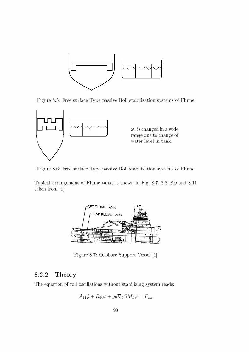
Figure 8.5: Free surface Type passive Roll stabilization systems of Flume
ωz is changed in a widerange due to change ofwater level in tank.
Figure 8.6: Free surface Type passive Roll stabilization systems of Flume
Typical arrangement of Flume tanks is shown in Fig. 8.7, 8.8, 8.9 and 8.11taken from [1].
Figure 8.7: Offshore Support Vessel [1]
8.2.2 Theory
The equation of roll oscillations without stabilizing system reads:
A44ϕ+B44ϕ+ %g∇0GMLϕ = Fϕϕ
93
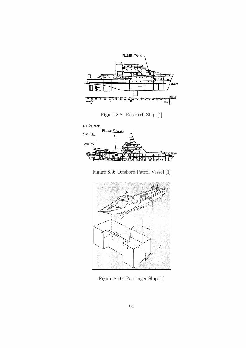
Figure 8.8: Research Ship [1]
Figure 8.9: Offshore Patrol Vessel [1]
Figure 8.10: Passenger Ship [1]
94
Figure 8.11: Reduction of the roll amplitude using the Flume tank designedby Hoppe Marine (taken from [1]).
A44 - effective mass moment of inertia
B44 - damping coefficient
Fϕϕ - wave induced forces
The equation of roll oscillations with stabilizing system reads:
(A44 +mTϕ)ϕ+ (B44 +NTϕ)ϕ+ (BTϕ + %g∇0GML)ϕ = Fϕϕ
mTϕ - effective mass moment of inertia of water in stabilizer unit
NTϕ - damping coefficient of stabilizer unit
BTϕ - restoring moment coefficient of stabilizer unit
The values mTϕ, NTϕ and BTϕ are related only to the difference between anactive stabilizer and a condition where the fluid is replaced by a solid masscorresponding to the frozen liquid.
A44ϕ+B44ϕ+ (%g∇0GML)ϕ = Fϕϕ − FTϕmTϕ · ϕ+NTϕϕ+BTϕϕ = FTϕ
95
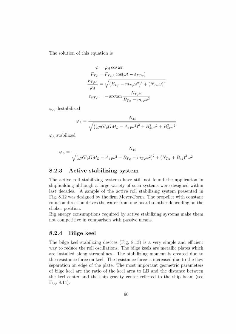
The solution of this equation is
ϕ = ϕA cosωt
FTϕ = FTϕA cos(ωt− εFTϕ)
FTϕAϕA
=
√(BTϕ −mTϕω2)2 + (NTϕω)2
εFTϕ = − arctanNTϕω
BTϕ −mtϕω2
ϕA destabilized
ϕA =N44√(
(%g∇0GML − A44ω2)2 +B244ω
2 +B244ω
2
ϕA stabilized
ϕA =N44√
(%g∇0GML − A44ω2 +BTϕ −mTϕω2)2 + (NTϕ +B44)2 ω2
8.2.3 Active stabilizing system
The active roll stabilizing systems have still not found the application inshipbuilding although a large variety of such systems were designed withinlast decades. A sample of the active roll stabilizing system presented inFig. 8.12 was designed by the firm Meyer-Form. The propeller with constantrotation direction drives the water from one board to other depending on thechoker position.Big energy consumptions required by active stabilizing systems make themnot competitive in comparison with passive means.
8.2.4 Bilge keel
The bilge keel stabilizing devices (Fig. 8.13) is a very simple and efficientway to reduce the roll oscillations. The bilge keels are metallic plates whichare installed along streamlines. The stabilizing moment is created due tothe resistance force on keel. The resistance force is increased due to the flowseparation on edge of the plate. The most important geometric parametersof bilge keel are the ratio of the keel area to LB and the distance betweenthe keel center and the ship gravity center referred to the ship beam (seeFig. 8.14):
96
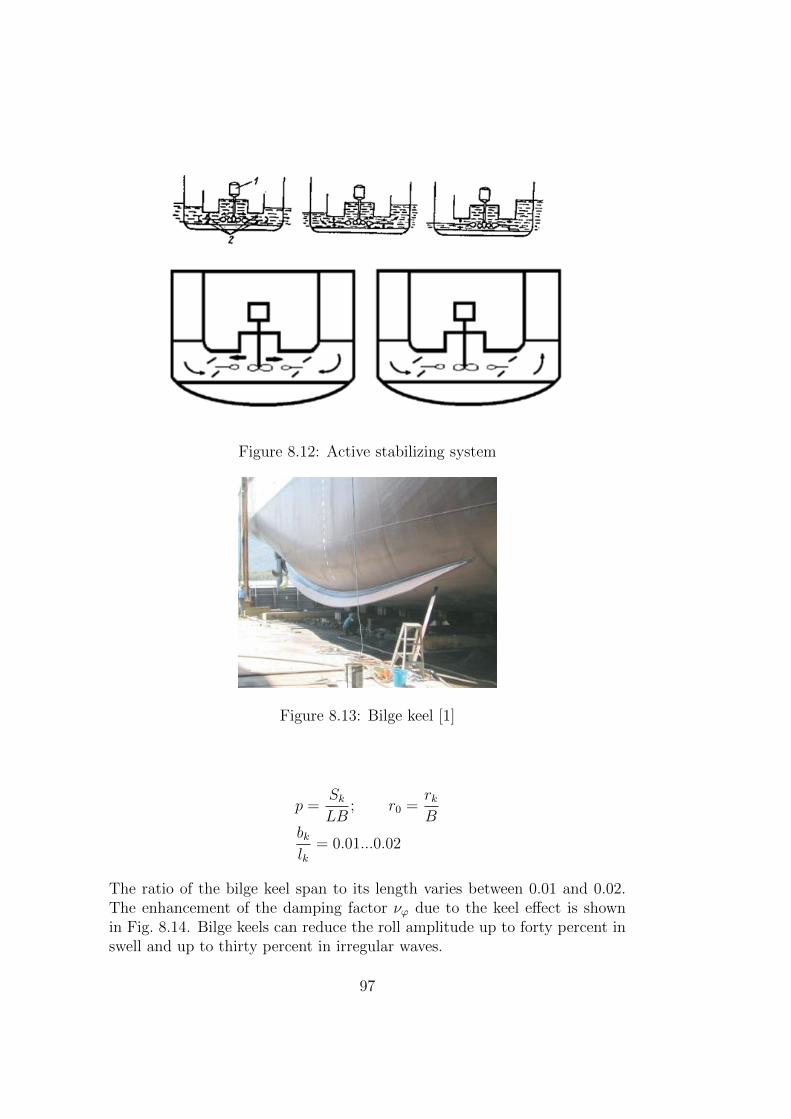
Figure 8.12: Active stabilizing system
Figure 8.13: Bilge keel [1]
p =SkLB
; r0 =rkB
bklk
= 0.01...0.02
The ratio of the bilge keel span to its length varies between 0.01 and 0.02.The enhancement of the damping factor νϕ due to the keel effect is shownin Fig. 8.14. Bilge keels can reduce the roll amplitude up to forty percent inswell and up to thirty percent in irregular waves.
97
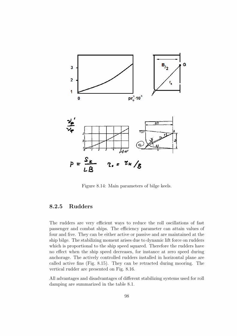
Figure 8.14: Main parameters of bilge keels.
8.2.5 Rudders
The rudders are very efficient ways to reduce the roll oscillations of fastpassenger and combat ships. The efficiency parameter can attain values offour and five. They can be either active or passive and are maintained at theship bilge. The stabilizing moment arises due to dynamic lift force on rudderswhich is proportional to the ship speed squared. Therefore the rudders haveno effect when the ship speed decreases, for instance at zero speed duringanchorage. The actively controlled rudders installed in horizontal plane arecalled active fins (Fig. 8.15). They can be retracted during mooring. Thevertical rudder are presented on Fig. 8.16.
All advantages and disadvantages of different stabilizing systems used for rolldamping are summarized in the table 8.1.
98
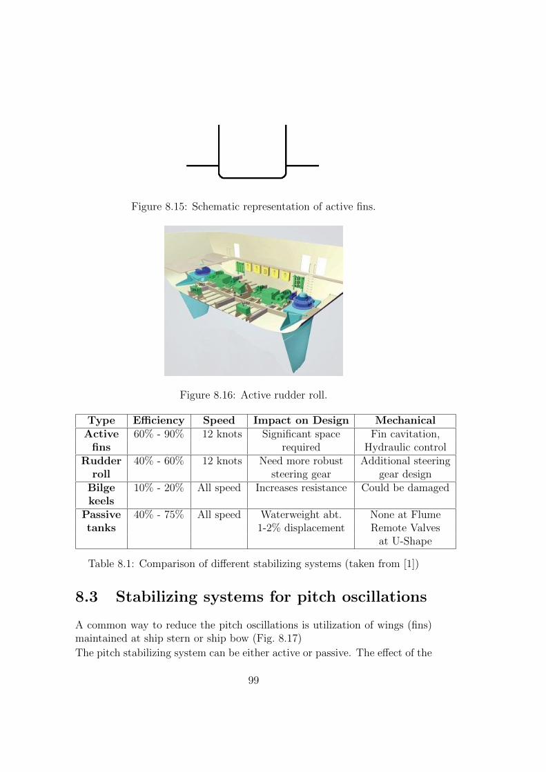
Figure 8.15: Schematic representation of active fins.
Figure 8.16: Active rudder roll.
Type Efficiency Speed Impact on Design MechanicalActive 60% - 90% 12 knots Significant space Fin cavitation,
fins required Hydraulic controlRudder 40% - 60% 12 knots Need more robust Additional steering
roll steering gear gear designBilge 10% - 20% All speed Increases resistance Could be damagedkeels
Passive 40% - 75% All speed Waterweight abt. None at Flumetanks 1-2% displacement Remote Valves
at U-Shape
Table 8.1: Comparison of different stabilizing systems (taken from [1])
8.3 Stabilizing systems for pitch oscillations
A common way to reduce the pitch oscillations is utilization of wings (fins)maintained at ship stern or ship bow (Fig. 8.17)
The pitch stabilizing system can be either active or passive. The effect of the
99
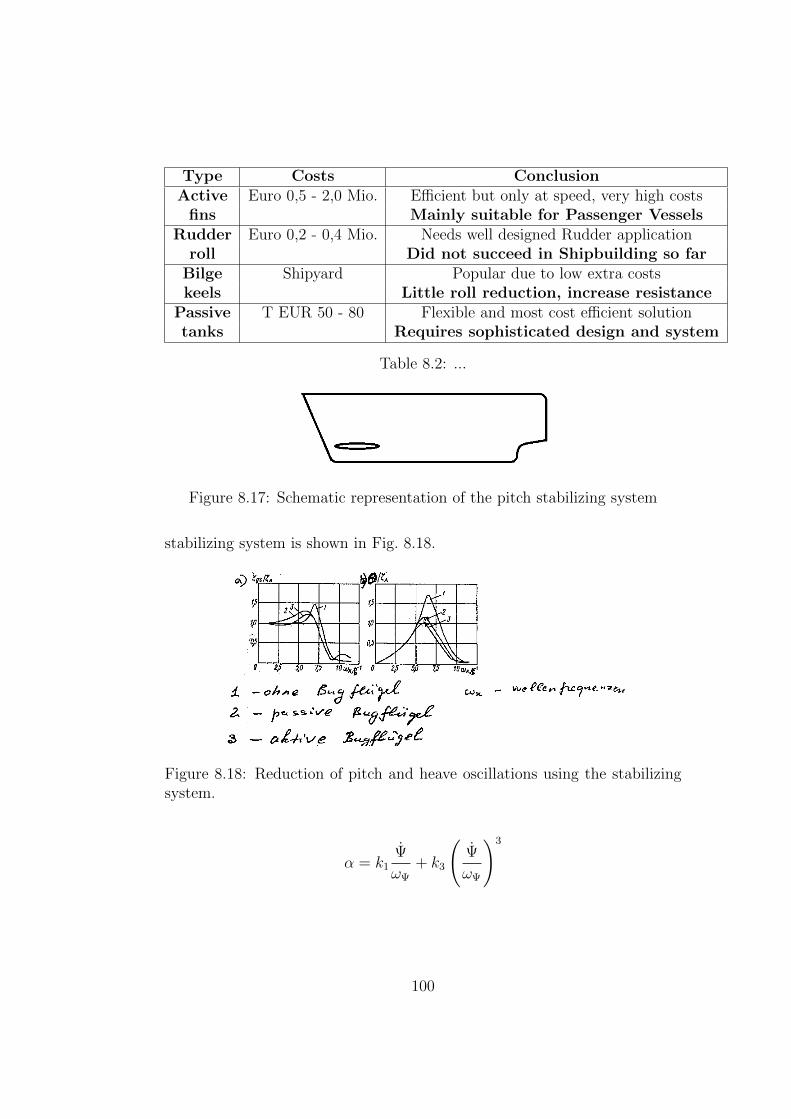
Type Costs ConclusionActive Euro 0,5 - 2,0 Mio. Efficient but only at speed, very high costs
fins Mainly suitable for Passenger VesselsRudder Euro 0,2 - 0,4 Mio. Needs well designed Rudder application
roll Did not succeed in Shipbuilding so farBilge Shipyard Popular due to low extra costskeels Little roll reduction, increase resistance
Passive T EUR 50 - 80 Flexible and most cost efficient solutiontanks Requires sophisticated design and system
Table 8.2: ...
Figure 8.17: Schematic representation of the pitch stabilizing system
stabilizing system is shown in Fig. 8.18.
Figure 8.18: Reduction of pitch and heave oscillations using the stabilizingsystem.
α = k1Ψ
ωΨ
+ k3
(Ψ
ωΨ
)3
100
Chapter 9
Parametric oscillations
Parametric oscillations arise when one of parameters characterizing the os-cillating system depends periodically on time. Parametric ship oscillationsarise due to periodic change of the metacentric height:
GMγ = GM0γ + AGM cosωt (9.1)
which is in previous chapters assumed to be constant, i.e.
GMγ = GM0γ .
The motion equation of free roll oscillations with variable metacentric heightis:
Ixxϕ+ A44ϕ−B44ϕ+ ρg∇0(GM0γ + AGM cosωt)ϕ = 0
or:
ϕ+ 2νϕϕ+ ω2ϕϕ = µϕ cosωtϕ,
where
νϕ =B44
2(Ixx + A44), ω2
ϕ =ρg∇0GM
0γ
Ixx + A44
µϕ =AGMρg∇0
Ixx + A44
(9.2)
Analyzing (9.2) one can state that change of the metacentric height can causethe perturbation moment resulting in parametric oscillations.Physical reason for the appearance of the additional perturbation moment is
101
the effect of the ship submergence change during roll and vertical oscillations.The change of the roll angle causes the moment:
ρ∇0gGMγϕ (9.3)
The change of the ship draught ξ results in an additional moment
ρg∇0AGM cosωtϕ
which is proportional to ζ and ϕ.
The equation (9.2) has no analytic solution in elementary functions. How-ever, properties of its solution are well known. It can be shown that if thefrequency of perturbation moment is twice as large as the free roll oscillationfrequency, i.e. ω = 2ωϕ, the parametric resonance takes place. Since theperturbation moment depends on heave ζ, the parametric resonance takesplace when the frequency of vertical oscillations is approximately twice aslarge as the frequency of roll oscillations. With the other words, during semiperiod of roll oscillations the heave change performs the full period oscillationas shown schematically on Fig. 9.1. The parametric resonance is typical forships with big distance between the center of gravity and water plane surface(Fig. 9.2).
For parametric oscillation it is necessary that ship is brought from the equi-librium state by a certain perturbation. The natural reason of such per-turbation for roll oscillations is beam seaway. However, the parametric rolloscillation can arise also in head waves. If the ship has a certain roll angle inhead waves, the hydrostatic lift force becomes larger at the wave crest andsmaller at wave valley. This results in a perturbation moment depending onroll angle.
This kind of parametric oscillations depends on the wave lengths and shiploading.
Periodic change of the metacentric height results in asymmetry of roll oscil-lations. Due to phase displacement between heave oscillations and waves δζthe averaged additional moment is different for positive and negative ϕ. Inthe resonance case of vertical oscillations ω ≈ ωζ , the middle roll angle is [9]
ϕ0 = κϕω2
gAzg − TGMγ
√Aκζ
2νζκT(9.4)
102
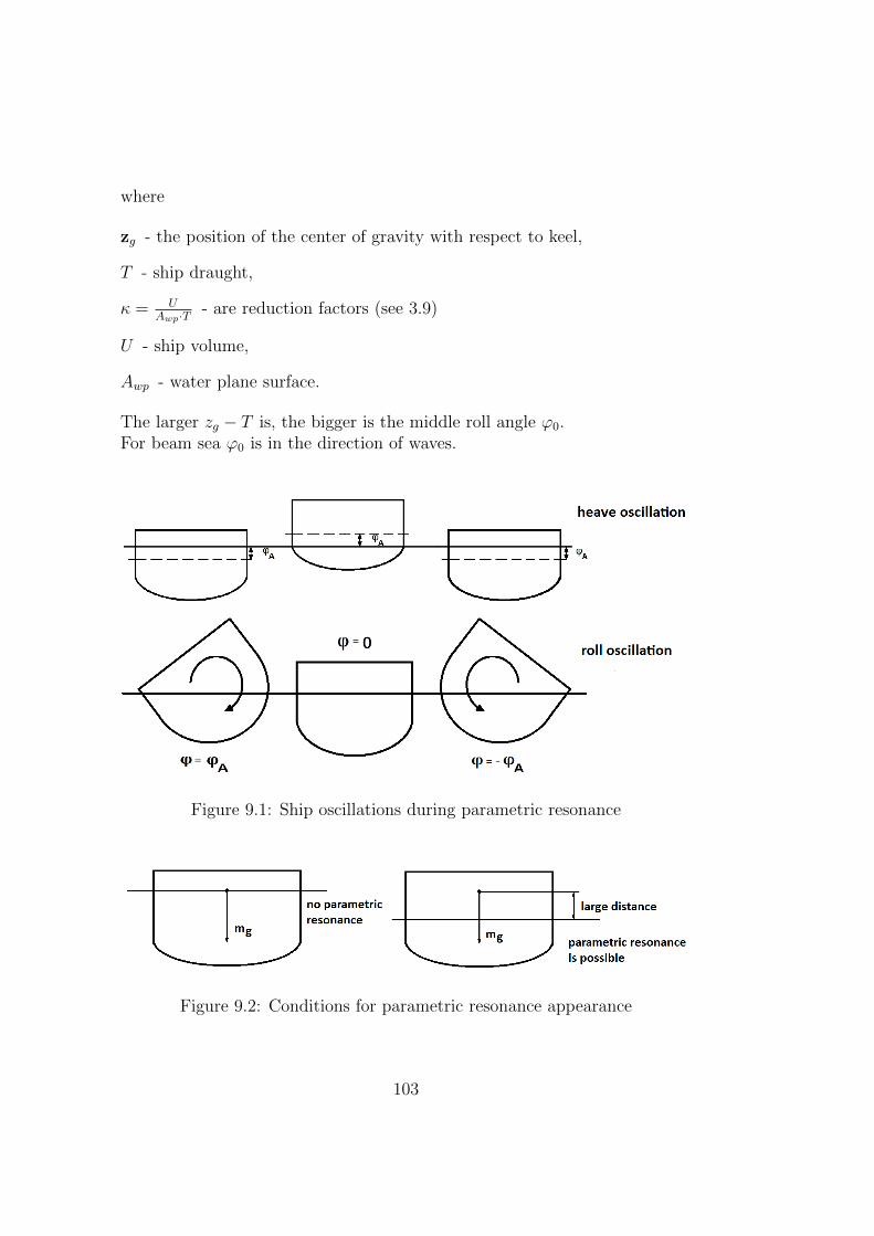
where
zg - the position of the center of gravity with respect to keel,
T - ship draught,
κ = UAwp·T - are reduction factors (see 3.9)
U - ship volume,
Awp - water plane surface.
The larger zg − T is, the bigger is the middle roll angle ϕ0.For beam sea ϕ0 is in the direction of waves.
Figure 9.1: Ship oscillations during parametric resonance
Figure 9.2: Conditions for parametric resonance appearance
103

104
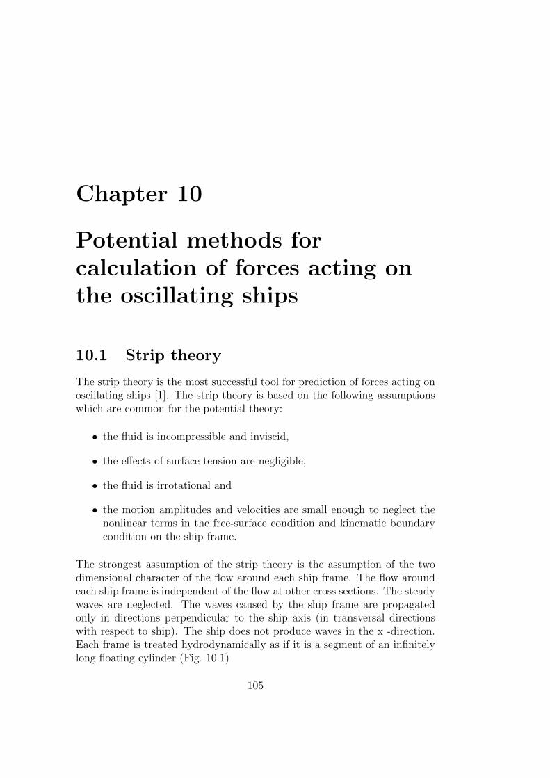
Chapter 10
Potential methods forcalculation of forces acting onthe oscillating ships
10.1 Strip theory
The strip theory is the most successful tool for prediction of forces acting onoscillating ships [1]. The strip theory is based on the following assumptionswhich are common for the potential theory:
• the fluid is incompressible and inviscid,
• the effects of surface tension are negligible,
• the fluid is irrotational and
• the motion amplitudes and velocities are small enough to neglect thenonlinear terms in the free-surface condition and kinematic boundarycondition on the ship frame.
The strongest assumption of the strip theory is the assumption of the twodimensional character of the flow around each ship frame. The flow aroundeach ship frame is independent of the flow at other cross sections. The steadywaves are neglected. The waves caused by the ship frame are propagatedonly in directions perpendicular to the ship axis (in transversal directionswith respect to ship). The ship does not produce waves in the x -direction.Each frame is treated hydrodynamically as if it is a segment of an infinitelylong floating cylinder (Fig. 10.1)
105
Figure 10.1: Assumption of the strip theory [1].
Usually the ship is subdivided into 20 or 30 cross sections treated sequentially.For the zero forward speed case, interactions between the cross sections areignored.
Such assumptions are valid for slender bodies with the length to the breadthratio larger than at least seven. However, the experience has shown thatstrip theory can be applied successfully for floating bodies with a length tobreadth ratio larger than three [1], at least from a practical point of view.The two-dimensional nature of the problem implies three degrees of freedomof motion:
• vertical or heave,
• horizontal or sway and
• rotational about a horizontal axis or roll.
The forces δFi acting on each frame are then summed to get the full force:
Fi =
L∫0
δFidx
Where i is the force direction (2 or 3, sway or heave). The yaw and pitchmoments are calculated by multiplication of corresponding forces with arm x:
M5 = −L∫
0
xδF3dx, M6 =
L∫0
xδF2dx
106
The rolling moment is just the sum of frame moments
M4 =
L∫0
δM4dx
The ship frame is forced into harmonic motion ζj cosωt, j = 2, 3 and 4.The velocity potential Φj(x, y, t) = Re{ϕj(x, y)exp[−iωt]} should satisfy thefollowing conditions
• Laplace equations in the whole domain
∂2Φj
∂x2+∂2Φj
∂z2= 0 (10.1)
• Linearized mixed condition on the free surface at y=0
∂2Φj
∂t2+ g
∂Φj
∂z= 0 (10.2)
• No penetration condition at the frame surface
~n∇Φj = Un (10.3)
where ~n is the unit vector normal to the ship surface and Un is the normalcomponent of the ship surface velocity. The no penetration condition issatisfied at the mean (rest) position of the ship frame.
• Decay condition far from the ship
Φj−−−−→z →∞ = 0 (10.4)
• The radiation condition that the disturbed surface of the fluid takesthe form of regular progressive outgoing gravity waves at large distancefrom the ship
Wehausen and Laitone [2] derived the source pulsating under the free surfacewhich has the potential
H(y, z, ξ, η, t) = Re{G(z, ζ, t) · e−i·ω·t} (10.5)
where
107
G(z, ζ) =1
2 · π·Re
{ln(z − ζ)− ln(z − ζ) + 2 · p.v.
∞∫0
e−i·k·(z−ζ)
ν − kdk
}
− i ·Re{ei·ν·(z−ζ)
}z = y + i · z ζ = ξ + i− η ζ = ξ − i · η ν = ω2/g
The potential (10.5) satisfies the conditions (10.1), (10.2), (10.4) and the ra-diation condition. The only condition to be satisfied is the no penetrationcondition (10.3).
The sources (10.5) are distributed over the ship frame surface C0:
Φj(y, z, t) = Re
{∫Co
Q(s) ·G(z, ζ) · e−i·ω·t · ds}
where C0 is the submerged contour of the cylindrical cross section at its mean(rest) position and Q(s) represents the complex source density as a functionof the position along C0.The intensity Q(s) is determined from the no penetration condition
Re
{(~n · ~∇) ·
∫C0
Q(s) ·G(z, ζ) · ds} = 0
Im
{(~n · ~∇) ·
∫C0
Q(s) ·G(z, ζ) · ds}
= ζm · ω · n(m)
(10.6)
where ζm denotes the amplitude of oscillation and n(m) the direction cosineof the normal velocity at z on the cylinder. Both ζm and n(m) depend on themode of motion.
Equation (10.6) is applied at the midpoints of each of the N segments and itis assumed that over an individual segment the complex source strength Q(s)remains constant, although it varies from segment to segment. With thesestipulations, the set of coupled integral equations (Equation (10.6)) becomesa set of 2N linear algebraic equations in the unknowns:
Re
{Q(m)(sj)
}= Q
(m)j and lm
{Q(m)(sj)
}= Q
(m)N+j
108
Thus, for i = 1, 2, ..., N :
+N∑j=1
{Q
(m)j · I(m)
ij
}+
N∑j=1
{Q
(m)N+j · J
(m)ij
}= 0
−N∑j=1
{Q
(m)j · J (m)
ij
}+
N∑j=1
{Q
(m)N+j · I
(m)ij
}= ω · ζm · n(m)
i
The hydrodynamic pressure at (yi, zi) along the cylinder is obtained from thevelocity potential by means of the linearized Bernoulli equation:
p(m)(yi, zi, ω, t) = −ρ · ∂Φ(m)
∂t(yi, zi, ω, t)
as:
p(m)(yi, zi, ω, t) = p(m)a (yiziω) · cos(ω · t) + p(m)
ν (yi, zi, ω) · sin(ω · t)
where p(m)a and p
(m)ν are the hydrodynamics pressure in-phase with the dis-
placement and in-phase with the velocity, respectively and ρ denotes thedensity of the fluid.
M (m)(ω) = 2 ·N∑i=1
{p(m)a (yi, zi, ω) · n(m)
i · |si|}
N (m)(ω) = 2 ·N∑i=1
{p(m)ν (yi, zi, ω) · n(m)
i · |si|}
for the added mass and damping forces or moments, respectively.
10.2 Principles of Rankine source method for
calculation of seakeeping
10.2.1 Frequency domain simulations
Generally there are two basic methods of simulation of time dependent pro-cesses. In the first method called the simulation in frequency domain theunsteady process is considered as the sum of the mean part which is timeindependent and the periodical part. The mean part can be calculated using
109
nonlinear strategy, i.e. the seeking parameters depends on ship kinematicparameters in non linear manner. The periodic part is considered as smalland found from a linear theory. This formalism is based on Fourier analysisof unsteady processes. The strip theory described above is the sample of thefrequency domain simulation. Each unsteady quantity q is represented inform:
q = q0 + qeiωt (10.7)
where
q0 is the mean value,q is amplitude andω is frequency.
The potential around the ship is represented as the sum of four terms [13]
ϕ = (−V x+ ϕs) + (ϕw + ϕI) (10.8)
where
−V x potential of incident uniform flow along the x- axis,V ship speed,ϕs potential of the steady flow disturbance,ϕw potential of incident wave,ϕI remaining unsteady potential.
The terms in the first parenthesis describes the steady flow around the shipwith account for free surface effects. The second parenthesis represent theperiodic flow due to waves. Determination of the potential (−V x + ϕs)is discussed in the wave resistance potential theory. This problem can besolved utilizing either a full nonlinear or a linear formalism. Numerical linearmethod for two dimensional case is described in Chapter 6.7 ([7]). Theboundary conditions for ϕI are linearized. The following boundary conditionsshould be satisfied [13]:
• no penetration on the hull,
• kinematic boundary condition on the free surface,
• dynamic boundary condition on the free surface,
• decay of disturbances far away from the ship,
110
• radiation condition.
The Laplace equation and decay condition are automatically satisfied withinthe Rankine source method. The unsteady potential is decomposed intoradiation ϕi and diffraction components ϕd:
ϕI =6∑i=1
ϕiui + ϕd (10.9)
where ui - ship velocities (both translational and angular).For the sake of simplicity we consider fully linear formalism (∇ϕs and ∇ϕIare small). The kinematic and dynamic boundary conditions are used toderive mixed boundary condition on the free surface.The dynamic boundary condition written in the inertial reference system is(see page 110 in [7])
∂ϕ
∂t0+
1
2
[(∂ϕ
∂x
)2
+
(∂ϕ
∂y
)2
+
(∂ϕ
∂z
)2]
+ gz = 0 (10.10)
Its linear version is
∂ϕ
∂t0+ gz = 0 at z = ζ (10.11)
The relation between the derivative on time in inertia ∂ϕ/∂t0 and ship fixedcoordinate system ∂ϕ/∂t is
∂ϕ
∂t0=∂ϕ
∂t− ~V∇ϕ (10.12)
where ~V is the speed of the reference system (speed of ship). Substitut-ing (10.12) into (10.11) we obtain:
∂ϕ
∂t− ~V∇ϕ+ gz = 0, at z = ζ (10.13)
The linearized version of the kinematic boundary conditions (see page 111in [7]) reads:
∂ζ
∂t0=∂ϕ
∂zat z = ζ (10.14)
Differentiating (10.11) on time
∂2ϕ
∂t20+ g
∂ζ
∂t0= 0 (10.15)
111
and substituting (10.14) into (10.15) one obtains
∂2ϕ
∂t20+ g
∂ϕ
∂z= 0 (10.16)
Using the relation
∂
∂t0=
∂
∂t− ~V∇
we get
∂2ϕ
∂t20=
∂
∂t0
(∂ϕ
∂t0
)=
∂
∂t0
(∂ϕ
∂t− ~V∇ϕ
)=
=∂
∂t
(∂ϕ
∂t− ~V∇ϕ
)− ~V∇
(∂ϕ
∂t− ~V∇ϕ
)=
=∂2ϕ
∂t2− ~V∇∂ϕ
∂t− ~V∇∂ϕ
∂t+ ~V 2∇2ϕ =
=∂2ϕ
∂t2− 2~V∇∂ϕ
∂t
The mixed boundary condition (10.16) in the ship fixed system reads
∂2ϕ
∂t2− 2~V∇∂ϕ
∂t+ g
∂ϕ
∂z= 0 (10.17)
Substituting ϕ = ϕ0+ϕ1, where ϕ0 = −V x+ϕs and ϕ1 = ϕw+ϕI into (10.17)one obtains
∂2ϕ1
∂t2− 2~V∇∂ϕ
1
∂t+ g
∂ϕ1
∂z+ g
∂ϕ0
∂z= 0 (10.18)
Since ϕ1 = ϕ1eiωt, the Eq. (10.18) takes the form:
−ω2ϕ1 − 2iω~V∇ϕ1 + g∂ϕ1
∂z+ g
∂ϕ0
∂ze−iωt = 0
Within the fully linear formalism developed further in this section ∂ϕ0
∂z= 0
at the free surface. Therefore the problem is reduced to the problem withrespect to amplitudes ϕI since ϕw is given
ϕw = Re(−icAe−ik(x cosµ−y sinµ)eiωt)
The equation for amplitudes reads
112
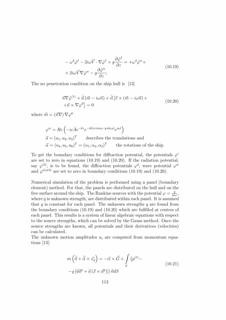
− ω2ϕI − 2iω~V · ∇ϕI + g∂ϕI
∂z= +ω2ϕw+
+ 2iω~V∇ϕw − g∂ϕw
∂z;
(10.19)
The no penetration condition on the ship hull is [13]
~n∇ϕ(1) + ~u (~m− iω~n) + ~α [~x× (~m− iω~n) +
+~n×∇ϕ0]
= 0(10.20)
where ~m = (~n∇)∇ϕ0
ϕw = Re(−icAe−kze−ik(x cosµ−y sinµ)eiωt
)~u = (u1, u2, u3)T describes the translations and
~α = (u4, u5, u6)T = (α1, α2, α3)T the rotations of the ship.
To get the boundary conditions for diffraction potential, the potentials ϕi
are set to zero in equations (10.19) and (10.20). If the radiation potential,say ϕ(3), is to be found, the diffraction potentials ϕd, wave potential ϕw
and ϕi(i 6=3) are set to zero in boundary conditions (10.19) and (10.20).
Numerical simulation of the problem is performed using a panel (boundaryelement) method. For that, the panels are distributed on the hull and on thefree surface around the ship. The Rankine sources with the potential ϕ = q
4πr,
where q is unknown strength, are distributed within each panel. It is assumedthat q is constant for each panel. The unknown strengths q are found fromthe boundary conditions (10.19) and (10.20) which are fulfilled at centres ofeach panel. This results is a system of linear algebraic equations with respectto the source strengths, which can be solved by the Gauss method. Once thesource strengths are known, all potentials and their derivatives (velocities)can be calculated.The unknown motion amplitudes ui are computed from momentum equa-tions [13]:
m(~u+ ~α× ~xg
)= −~α× ~G+
∫S
(p(1)−
−% [~u~ag + ~a (~x× ~ag)])~ndS(10.21)
113

m(~xg × ~u
)+ I~α = − ~xg ×
(~α× ~G
)+
+
∫ (p(1) − % [~u~ag + ~α (~x× ~αg)]
)× (x× a) dS
(10.22)
~xg center of gravityG = mg ship weightI matrix of the moments of inertia of the ship
M =
m 0 0 0 mzg 00 m 0 −mzg 0 mxg0 0 m 0 −mxg 00 −mzg 0 Ixx 0 −Ixzmzg 0 −mxy 0 Iyy 0
0 mxg 0 −Ixz 0 −Izz
Ixx =∫
(y2 + z2)dm, Ixz =∫xzdm
I =
Ixx 0 −Ixz0 Iyy 0−Ixz 0 −Izz
~a = (∇ϕ0∇)∇ϕ0
~ag = ~a− {0, 0, g}τ
The harmonic pressure p(1) is decomposed into parts due to incident wave,due to diffraction, and due to radiation.
p(1) = pw + pd +6∑i=1
piui
The components pi can be calculated from the linearized Bernoulli equation:
pi = −%(∂ϕi
∂t+∇ϕ0∇ϕi
)Two momentum vector equations (10.21) and (10.22) form a linear systemof six equations for the six motions ui which can easily be solved.
114
10.2.2 Time domain simulation (TDS)
Time domain simulations are performed to take the nonlinear effect at largeamplitude oscillations into account. Seaway is computed as superposition ofelementary waves using the following rules [13]:
• The wave frequencies ωj are chosen such that the area under the seaspectrum between ωj and ωj+1 is the same for all j. This results inconstant amplitudes for all elementary waves regardless of frequency.
• The frequency interval for simulation is divided into subintervals. Thesesubintervalls are larger where Sζ or the important RAOs are small andvice versa. In each subinterval a frequency ωj is chosen randomly (basedon constant probability distribution). Encounter angles are chosen ran-domly.
The frequencies, encounter angles, and phase angles chosen before the simu-lation must be kept during the whole simulations.
Numerical simulation of the problem is performed using panel (boundaryelement) method. For that, the panels are distributed on the hull and on thefree surface around the ship. The Rankine sources with the potential ϕ = q
4πr,
where q is unknown strength, are distributed within each panel. It is assumedthat q is constant for each panel. The unknown strengths q are found fromthe nonlinear boundary conditions on the free surface and no penetrationcondition which are fulfilled at centres of each panel both on ship surfaceand wave surface. This results is a system of linear algebraic equationswith respect to the source strengths, which is solved by the Gauss method.Once the source strengths are known, all potentials and their derivatives(velocities) can be calculated.The computation proceeds from the time step t to the step t + ∆t. Ateach time step t, the hydrodynamic forces are first calculated, which thenare substituted into the nonlinear motion equations. Once the kinematicparameters of the ship are computed from the motion equations, the nexttime step t+ ∆t is treated.
115

116
Bibliography
[1] Winkler S. Flume passive anti-roll tanks. application on merchant andnaval ships. presentation at the University of Rostock, 2012.
[2] Brix J. Manoeuvring technical manual. Seehafen Verlag, 1993.
[3] Kleinau D. Theorie des Schiffes, Manuskript. University of Rostock,2001. (in German).
[4] Makov J. Ship oscillations. Kaliningrad, 2007.
[5] http://www.marin.nl/web/Facilities-Tools/Basins/Seakeeping-Manoeuvring-Basin/Seakeeping-and-manoeuvring-basin-pdf.htm.
[6] Kornev N. Ship Theory I (ship manoeuvrability). 2011. Manuscript.
[7] Kornev N. Schiffstheorie I, page 162 S.
[8] Newman J. Marine hydrodynamics. MIT Press, 1984.
[9] Sisov V. Ship Theory. Odessa, 2004.
[10] Price W.G. and Bishop R.E. Probabilistic theory of ship dynamics.Halsted, London, 1974.
[11] Vugts J.H. The hydrodynamic coefficients for swaying, heaving androlling cylinders in a free surface. Int. Shipbuilding Progress, 15:pp. 224–276, 1968.
[12] Frahm H. Results of trials of the anti-rolling tanks at sea. Trans. of theInstitution of Naval Architects, Vol.53, 1911.
[13] Bertram V. Practical ship hydromechanics, page 270 p. Butterworth-Heinemann, 2000.
117