FACULTY OF ENGINEERING AND SUSTAINABLE DEVELOPMENT

NUMERICAL STUDY OF 2D PARTICLE FLOW IN A DUCT

Abolfazl Hayati

May 2012

Master’s Thesis in Energy Systems Master program in Energy Systems

Examiner: Taghi Karimipanah

Supervisor: Mathias Cehlin

Preface

First of all I am so thankful to the God who is so beneficent and merciful to me and never let me alone during my life.

I would like to thank my darling family, with their support I made this journey up to here.

I want to show my gratitude to my kind supervisor, Mathias Cehlin, which I spent wonderful time with him during the project and his comments promoted me to accomplish the thesis.

Beside I appreciate my examiner and kind teacher Professor Taghi Karimipanah, as well as Shahriar, my teacher and kind friend, and all HIG teachers during my master program; their guidance and commitment was always worth full and encourage me to go forward.

Also I should appreciate my previous teachers, and all my friends, especially Mohammad who helped me a lot during the thesis.

Abstract

In this thesis 2D CFD simulation of solid-gas multiphase flows was performed using Eulerian model with Dense Discrete Phase Model. Solid particles were injected in a duct and the particle flow pattern in the duct was studied. The main objective was to numerically investigate the effects of restitution coefficient, particle density and air velocity on particle motion, using the Eulerian model with dense discrete phase model. Different particle size distributions were also examined through different particle outlets in the duct. ANSYS FLUENT 14 was used for the CFD simulation. Different normal wall-particle restitution coefficient, particle density and air flow patterns were investigated. The simulated normal restitution coefficients were 0.5, 0.8 and 0.9; particle densities were 1500 kg/m3, 2650 kg/m3 and 3000 kg/m3; air flow pattern had different inlet mean velocities of 18.4 m/s, 20.7 m/s and 23.9 m/s. Different parameters of the air flow such as velocity, dynamic pressure, total pressure, turbulent kinetic energy and turbulence intensity were examined as well as the track of the particles and their bouncing into the domain. It is concluded that the normal restitution coefficient of between 0.8 and 0.9 is closer to the reality and that the particle flow pattern is highly dependent on the particle density and on the length of the computational domain. Simulation and prediction of exact behaviour of the particles in solid-gas multiphase problems seems to need more complicated models which take into account the impact of the particles on each other and on the flow itself.

Contents Nomenclature ......................................................................................................................................... 1

1. Introduction .................................................................................................................................... 3

1.1 The aim ......................................................................................................................................... 4

2. Theory ............................................................................................................................................ 5

2.1. CFD introduction .................................................................................................................... 5

2.2. Governing equations ............................................................................................................... 6

2.2.1. Mass conservation .......................................................................................................... 6

2.2.2. Momentum conservation ................................................................................................ 6

2.2.3. Energy conservation equation ........................................................................................ 7

2.2.4. Navier Stokes equations ................................................................................................. 8

2.2.5. Reynolds averaged equations ......................................................................................... 9

2.3. Turbulence ............................................................................................................................ 10

2.4. Turbulence intensity ............................................................................................................. 11

2.5. Turbulence models ............................................................................................................... 12

2.5.1. RANS models ............................................................................................................... 12

2.5.2. Large Eddy Simulation (LES) ...................................................................................... 15

2.5.3. Direct Numerical Simulation (DNS) ............................................................................ 15

2.6. Multiphase introduction........................................................................................................ 16

2.7. Approaches for multiphase modeling ................................................................................... 17

2.7.1. The Euler-Euler approach ............................................................................................. 17

2.7.2. The Eulerian model ...................................................................................................... 18

2.7.3. The VOF model ............................................................................................................ 18

2.7.4. The mixture model ....................................................................................................... 18

2.7.5. One-Way and Two-Way Coupling ............................................................................... 19

2.7.6. Dense discrete phase model .......................................................................................... 21

2.8. Interaction of the particles on turbulence ............................................................................. 22

2.9. Restitution coefficient .......................................................................................................... 26

2.9.1. Restitution coefficient theory ....................................................................................... 26

2.9.2. Fluent wall boundary conditions .................................................................................. 30

3. Process (method) .......................................................................................................................... 33

3.1. Gambit setup (Grid) ............................................................................................................. 33

3.2. Fluent setup .......................................................................................................................... 33

4. Results and discussion ................................................................................................................. 35

4.1. Grid dependency: ................................................................................................................. 35

4.2. Effect of air velocity ............................................................................................................ 37

4.2.1. Particle velocity tracks ................................................................................................. 49

4.3. Effect of particle density ...................................................................................................... 52

4.4. Effect of restitution coefficient ............................................................................................ 55

4.5. More injection ...................................................................................................................... 58

4.6. The chart for track of particles ............................................................................................. 59

5. Conclusions ...................................................................................................................................... 61

References ............................................................................................................................................ 63

1

Nomenclature In this thesis, the International System of units (SI) is used.

c Heat capacity

𝐶𝜇,𝜎𝑘,𝜎𝜀, 𝐶1𝜀 and 𝐶2𝜀 Constants of 𝑘 − 𝜀 model

𝐸𝑖𝑗 Average rate of deformation

𝑒𝑛 Normal restitution coefficient

𝑒𝑡 Tangential restitution coefficient

g Gravity constant

I Turbulence intensity

i Internal energy

K Mean kinetic energy

k Heat conductivity

k Turbulence kinetic energy

l length scale

p Pressure

Re Reynolds number

SE source term due to energy

SM Body forces

t Time (s)

U Mean velocity

u The instantaneous velocity in the x-direction

u´ Fluctuating velocity

𝑉𝑛 Normal velocity components

2

𝑉𝑡 Tangential velocity components

v The instantaneous velocity in the y-direction

w The instantaneous velocity in the z-direction

𝑊𝑘𝑖𝑛,𝑅 Kinetic energy released during the restitution

𝑊𝑘𝑖𝑛 Initial kinetic energy

Greek symbols 𝝐 Mean rate of dissipation per unit of fluid mass

𝜗 Velocity scale

υ Kinematic viscosity

τ Kolmogrov time scale

τ Shear stress

ρ Density (kg/m3)

μt Eddy viscosity

μ Dynamic viscosity

λ Kolmogrov length scale

λ Second viscosity

θ Temperature

ε Viscous dissipation rate

δij Kronecker delta

ß Particulate loading

Ratio between material densities

∆ Gradient

3

1. Introduction

Turbulent flows are of the most occurring and complicated cases in the nature, and when another phase is added, the flow become multiphase and much more complex. And turbulence may damp or increase by the effect of particles (Brennen, 2005).

Investigating on multiphase phenomena has been initiated from 1970s; Hetsroni (1989) and Crow, et al. (1998) used LDA (Laser Doppler Anemometry) measurements and first calculations of multiphase flows by direct numerical simulation (DNS) for low Reynolds numbers.

Gore and Crowe (1989) investigated the turbulence intensity (caused by adding the particles to the single flow in the computational domain); The measurement were done for a broad range of turbulent jet flows and pipes including all combinations of gas, liquid and solid flows with density ratios between 0.001 and 7500, volume fractions between 2.5𝑒−6and 0.2, and Reynolds number between 8000 and 100 000. They reported, small particles (relative to the turbulent length scale) follow the turbulent motions and get energy from turbulent motions of the fluid.

In case of large particles, since they do not tend to follow the turbulent motions, turbulence is increased by the wakes (caused by the relative motions) (Parthasarathy and Faeth, 1990).

The relation between the turbulent and the relative motion was studied also by Yuan and michaelides (1992) and Kenning and Crowe (1997).

Particle intensity is also effective on the turbulent intensity; Paris and Eaton (2001) has been examined the relation between the particle mass fraction and the change in the turbulent kinetic energy for a channel with glass sphere as particles.

Peiano, et al. (2001) and Cammarata et al. 2003 recommended that when nature of the flow is close to two dimensional, 2D CFD simulation is appropriate to apply.

Restitution coefficient has been studied mainly in granulation to produce granules in detergents, food, pharmaceuticals or fertilizers industry (Mörl, et al. 2007). The restitution coefficient can demonstrate how much of kinetic energy dissipates through a collision (van Buijtenen, et al. 2009). They simulated flow regimes such as spouting with aeration, jet in fluidized bed and intermediate spouting with different restitution coefficients between 0.2 to 0.97 with Aluminum oxide particles and aluminum walls. They also tested some free fall experiments to measure the granule restitution coefficient. Some granules were released from specified height with zero initial velocity and with different angle of incidence; they record the relative velocities before and after impact and calculate the ratio between them, i.e. restitution coefficient.

4

Bettega et al. (2009b; c) examined the solids behavior on the flat walls by using the Eulerian-Eulerian 3D model. They also compared the numerical results with experimental data; Bettega et al. (2009a) also used CFD simulation and verified it.

Wang et al. (2009) modeled hydrodynamics of a high flux circulating fluidized bed and they concluded that restitution coefficient is not critical in case of spouted bed flows and Restitution coefficient between 0.8 and 1 is normally used (Lan, et al. 2011).

1.1 The aim In this thesis the aim is investigating the effect of restitution coefficient, the particles density and the air flow velocity on the particle flow pattern in a duct. Three different normal wall-particle restitution coefficients of 0.5, 0.8 and 0.9 were investigated, particle densities of 1500 kg/m3, 2650 kg/m3 and 3000 kg/m3 were simulated and finally different air profiles with inlet mean velocity of 18.4m/s, 20.7m/s and 23.9m/s were examined in a channel. The main objective was to numerically investigate the effects of restitution coefficient, particle density and air velocity on particle motion, using the Eulerian model with dense discrete phase model. Particles injected to the computational domain and some simulations with different air Velocity, particle-wall normal restitution coefficient and different particle density were done by ANSYS FLUENT under the license of HIG. Some parameters such as particle velocity tracks, air velocity, air pressure, mixture turbulence intensity and turbulence kinetic energy were investigated as well.

5

2. Theory

2.1. CFD introduction

Computational fluid dynamics (CFD) is the system analysis including the fluid flow, heat transfer, chemical reactions with the computer aided simulation (Versteeg and Malalasekera, 1995). CFD can be applied for a wide range of processes and applications in industry or in academic researches. Examples of applying CFD includes aircraft or car aerodynamics, ship hydrodynamics, gas turbines, combustion in boilers or in engines, turbomachinery, cooling devices such as impinging jets, multiphase modeling, building environment, ventilation, weather prediction, biomedical engineering, city environment, meteorology and etc (Karimipanah, 1995).

In compare with doing experiment, CFD simulation is less expensive and time consuming. And also the experiment costs are also variable since they depend on the number of the configurations and data needed. In General CFD can reduce the cost and time of the new systems and designs; CFD is able to study different parameters on the systems which may not be easy to be done by the experiments; also in some cases it is dangerous to test some parameters over the safety limitations of the system but it is easy to do with simulation; also in CFD more detailed results can be gained. CFD simulation can be used for improving the design and optimizing different processes and devices working with fluid flows. Day by day using CFD is becoming more common in industry as well as in the academic level and research projects dealing with fluid dynamics since it is more cost and time effective to do simulation with CFD before making experiments with the real case or prototype. And sometimes it is obligatory when there is no possibility to do measurements. But still in most cases of simulation, validation is needed through related measurements which should be done to verify the simulation or the model. And sometimes it is not possible to do the measurement on a full scale size and measurements will be done on a model or prototype which is smaller or much smaller than the real full size. After verification step, if the measurements verify the simulation result, then the model for simulation can be used furthermore. For doing CFD simulation it is needed to have fundamental knowledge in fluid dynamics, heat transfer and thermodynamics as well as related experience to analyze the results. The software programs and codes using CFD, use the same turbulence models and in this thesis ANSYS Fluent is used under the license of HIG.

CFD codes are based on some numerical algorithms and consist of three different parts of preprocessor, solver and postprocessor. In the preprocessor the inputs of the ongoing problem are given to the CFD program by means of an easy to use interface. The inputs include the computational domain geometry, the grid and mesh of the computational domain cells, choosing the phenomena that aimed to be modeled, the fluids properties and finally the boundary conditions.

6

In the solver part, the unknown variables approximated as some initial values for the governing equations and then the equations are solved through different models and mathematical functions.

In the post processing part different information can be gained such as diagrams, contours, domain geometry, vector plots, surface plots and particle tracking. Diagrams and the information include temperature, pressure, velocity, volume fraction and etc at any point of the computational domain.

It is important to mention that in the multiphase simulation still research is keeping on and although multiphase is so common in the nature; it is not fully developed or modeled by the current simulation models just like the most of other natural phenomena. But it was tried to get realistic results in 2D CFD simulation of solid-gas multiphase.

2.2. Governing equations

The governing equations are mathematical explanation of the conservation laws of physics (Versteeg and Malalasekera, 1995):

1) The fluid mass is conserved. 2) According to Newton’s second law on a fluid particle or control volume summation

of the forces are equal to the rate of the momentum change. 3) According to the first law of thermodynamics the rate of energy change equals to the

heat rate added to the control volume or the fluid particle and the rate of the work done on the fluid particle.

2.2.1. Mass conservation According to the mass conservation, the rate of the mass increase in fluid element is equal to the net rate of the flow into the fluid element. For the compressible flow this can be formulated as follows and is called the continuity equation for an unsteady compressible fluid at a point:

(2.1)

The first term is the rate of the density change per time and the second term is called the convective term and is the net mass flow crosswise the boundaries.

2.2.2. Momentum conservation According to the second law of Newton the net forces on a fluid particle is equal to the net momentum change of the particle. There are two kinds of forces on a fluid particle; body

7

forces such as gravity or Coriolis or centrifugal and surface forces such as pressure or viscous forces.

The momentum equation in the x direction:

(2.2)

The momentum equation in the y direction:

(2.3)

And the momentum equation in the z direction:

(2.4)

The SM terms are the representative of the body forces and u, v and w are the velocity components.

2.2.3. Energy conservation equation According to the law of thermodynamics the energy change rate for a fluid particle is the rate of work done on the fluid particle in addition to the heat added.

(2.5)

(2.6)

8

The term 𝐸 consists of internal energy 𝑖 and the kinetic energy. The 𝑆𝐸 term is the energy term related to a source. The term including the temperature gradient is the heat transfer to the fluid and the rest terms of the right side are the work done on the fluid particle.

When air flows in the channel the governing equations consist of continuity, momentum and energy equation. And the times averaged of those equations are as follows (in Cartesian): Continuity equation:

(2.7) Momentum equation:

(2.8) Energy equation:

(2.9) For solving these equations containing Reynolds stress terms and turbulence heat flux

(Li, 1994), turbulence models are used. In our case since it is isothermal, the terms consisting ∆Θ disappear, i.e. the last term in momentum equation and the whole energy equation.

2.2.4. Navier Stokes equations In order to close and solve the equations, the viscous stresses of 𝜏𝑖𝑗 must be modeled and this can be done in the Newtonian fluids by the linear relation of the rate of the deformation to the viscous stresses. And the relation coefficient is μ, i.e. the dynamic viscosity for relating the linear deformations to stresses and λ, i.e. the second viscosity to relate the volumetric deformations to stresses. In result the three dimensional tensor of viscous stress can be gained:

9

(2.10)

Then by substituting these viscous stresses to the momentum equations the Navier-Stokes equations can be gained:

𝑥-momentum:

(2.11)

𝑦-momentum:

(2.12)

𝑧-momentum:

(2.13)

The equations named of two 19th century scientists who derived the equations independently for the first time.

2.2.5. Reynolds averaged equations Since Navier-Stokes equations are too costly from time and computational point of view. So Navier-Stokes equations can be simplified to time-averaged ones which are called Reynolds equations. If supposed to be a property of the fluid, then the mean value of , which is can be defined:

(2.14)

And ; by applying these formulas to the Navier-Stokes equations, Reynolds equations can be gained:

10

(2.15)

In the transformation of the equations to the time averaged ones, six unknowns are obtained, the Reynolds stresses which must be modeled for closing and solving the equations. In order to solve these equations different turbulent models have been developed.

2.3. Turbulence

Fluids are laminar or turbulent, laminar regimes occur when there is no disruption in the fluid layers and they are parallel to each other.

Turbulent is hard to define exactly in words but it is easier to describe a turbulent flow and motion by its characteristics (Hinze, 1975); First of all a turbulent flow has variations in time and space which is called irregularity; Turbulent flow is chaotic and has its properties so that pressure or velocity stochastically changes and has rapid variation. A turbulent flow has three dimensions even if the mean flow considered being one or two dimensional. In all turbulent flows the kinetic energy is dissipating into heat which is called dissipativity caused by of the viscosity effect. In most cases for simplification, turbulence flows are approximated by a mean flow which will not exactly show the solution to a real turbulence flow. And an analytical solution for Navier Stokes equations is not possible (Karimipanah 1996). So instead of an analytical solution a numerical model can be used to solve the Navier Stokes equations. And in those turbulence models some approximations are applied to add up some equations and solve all needed variables.

The parameter indicating the turbulent is the Reynolds number which is the ratio of the inertia forces and viscous forces. Turbulence is not belonged to a special flow and occurs in high Reynolds numbers. And laminar flows occur in low Reynolds numbers. For example flows over a plate with Reynolds number less than 10000 are laminar and above this number they are turbulent.

Turbulent flows are always with some properties such as irregularity, randomness and chaotic motion. So the velocity is composed of two parts; one part is steady mean velocity 𝑈

11

and the other part is the related fluctuating part which both can be explained by Navier-Stokes equations.

(2.16)

Since all of the turbulent flows are much bigger than the molecular scale, they can be treated as a continuum. Also in turbulent flows, boundary layers spread with a more speed i.e. diffusivity increases. When flow become turbulent; momentum, heat transfer and mass transfer increases. Transformation of the kinetic energy of the smallest eddies to internal energy or dissipation occurs in all turbulent flows which are caused by friction or viscous forces. The smallest scales in which dissipation occurs are called Kolmogorov scales; including the velocity scale υ, the length scale η and the time scale τ. And they can be determined by energy dissipation rate ε and viscosity ν.

The largest eddies get energy from the mean flow and then they transfer kinetic energy to the smaller eddies or scales and the whole process of the energy transformation is called cascade process.

2.4. Turbulence intensity

Turbulence level or intensity is the ratio between the root mean square of the velocity fluctuation 𝑢′and the mean velocity U.

𝐼 = 𝑢′𝑈

(2.17)

Turbulent intensity usually described in percentage and thus the fraction will be multiplied by 100. Turbulent intensity can be derived from the turbulent kinetic energy as well according to the below formula:

𝑢′ = �13

(𝑢𝑥′2 + 𝑢𝑦′2 + 𝑢𝑧′2) = �2𝑘3

(2.18)

𝑈 = �𝑈𝑥2 + 𝑈𝑦2 + 𝑈𝑧2

(2.19)

In this project it is assumed that there is only one mean velocity component in the direction of the flow and the other ones are zero but fluctuating components of the velocity are assumed equal since turbulence is assumed isotropic, so the formula for the turbulence intensity 𝐼 can be gained as follows:

12

𝐼 = 𝑢′𝑈

=�2𝑘3

�𝑈𝑥2= √2𝑘

𝑈𝑥

(2.20)

For estimating the turbulence intensity as the boundary condition for CFD simulations, earlier experience and measurements can be used; for the high turbulence cases such as high speed flows in turbines and compressors a number between 5 and 20% can be used. For medium cases such as ventilation flows a number between 1 and 5% can be used and finally for the low turbulence ones such as external still standing flows around the cars, turbulence intensity is less than 1%.

2.5. Turbulence models

The turbulent models can be categorized in three main parts, Reynolds Averaged Navier-Stokes (RANS) models, Large Eddy Simulation (LES) and Direct Numerical Simulation (DNS).

1) Reynolds Averaged Navier-Stokes (RANS) models, in these models all fluid motions are not evaluated and since they are based on Reynolds equations, time averaged information such as flow properties can be gained through these models. Reynolds stress models (RSM), k-ε model and the mixing length model are of a type of RANS models.

2) Large Eddy Simulation (LES) models are the models which are not based totally on the Reynolds equation and they solve the largest scale fluid motions and approximate the smaller scales.

3) Direct Numerical Simulation (DNS) is the direct solution of the equations in which no approximation is involved and all the fluid motions are solved.

2.5.1. RANS models RANS models are less time consuming and do not need so much computational sources. RANS models are widely used for practical issues. 𝑘 − 𝜀 model is one of the RANS models and in the k-ε model, the boussinesq hypothesis is used to solve the Reynolds stresses i.e. the unknowns of the Reynolds equations. In Boussinesq hypothesis it is supposed that the Reynolds stresses are related to average rate of deformation. Based on this hypothesis, the average rate of deformation increases with the increase in Reynolds stresses:

(2.21)

In the k-ε model, the main point is the kinetic energy, and in a turbulent flow the instantaneous kinetic energy 𝑘(𝑡) is the summation of 𝐾 i.e. the mean kinetic energy and 𝑘 i.e. the turbulent kinetic energy:

13

(2.22)

In which:

(2.23)

(2.14)

The mean kinetic energy of the flow is as follows:

(2.25) In which E is the average rate of the deformation

(2.26)

And the turbulent kinetic energy will be;

(2.27)

The positive term in the mean kinetic energy equation and the same negative one in the turbulent kinetic energy show the conversion of kinetic energy from the mean value to the turbulent one. In addition to the equations for 𝑘, some equation is needed for viscous dissipation rate ε. Then the equations are used by 𝑘 − 𝜀 model to define length scale l and velocity scale 𝜗 for showing the large scale turbulence:

14

(2.28)

And here is the eddy viscosity:

(2.29) In which 𝐶𝜇 is a dimensionless constant. The transport equations for k and 𝜀 in the 𝑘 − 𝜀 model are as follows:

(2.30)

In the formulas above 𝐶𝜇,𝜎𝑘,𝜎𝜀, 𝐶1𝜀 and 𝐶2𝜀 are some constants that must be adjusted according to the turbulent flow range. In 𝑘 − 𝜀 model an extended Boussinesq relationship should be used for the Reynolds stresses:

15

(2.31) 𝑘 − 𝜀 model is one of the simplest established models and only initial and boundary conditions are needed and it is so practical in many engineering cases. On the other hand it has poor performance in some flows such as in swirling flows or flows with curved boundary layers. In fluent there is different type of 𝑘 − 𝜀 model such as standard 𝑘 − 𝜀 model, RNG and the realizable 𝑘 − 𝜀 model. 𝑘 − 𝜀 RNG model which was used for the air phase in this project has some advantages in compare with the standard 𝑘 − 𝜀 model; it is more accurate for the strained flows because of the term added in the 𝜀 equation, moreover the swirl effect is also added to RNG model. For Prandtl numbers in the RNG turbulence model there is an analytical formula which performs better than the user specified one in the standard 𝑘 − 𝜀 model.

2.5.2. Large Eddy Simulation (LES) In this kind of simulation the flow equations are space averaged (Ferziger, 1983). In large eddy simulation the small eddies have less energy than the large eddies and the small eddies are modeled and the larger ones are numerically and time dependently solved with the use of filtered Navier Stokes equations. By filtering which is precise Navier Stokes mathematical operation, those eddy smaller than the size of mesh or the filter will be removed. A more precise turbulent model should solve both the small and large eddies. So the parameter of the model is calculated in a dynamic way (Olsson, 1995) so that it is calculated in every grid point and every time step. LES models use spatial filtering and functions which do not need to be damped and the model parameters are space and time dependent (karimipanah, 1996). LES is much time consuming and needs too much computational effort but it is more accurate for large eddies. LES has been applied for so many cases effectively and it has its own applications.

2.5.3. Direct Numerical Simulation (DNS) In this kind of simulations there is no approximation or averaging, and with the aid of supercomputers they solve three dimensional dynamic and time dependent Navier stockes equations of the fluid flow. Since there is no approximation and errors to be controlled, DNS is the simplest one. In LES all the fluid motions and kinetic energy dissipations are considered and solved. The number of the grids on the mesh must be huge enough and the time step must be so small that the fluid particles could not pass one mesh cell size. The most time consuming and computationally costly approach is DNS but it has complete solution for the fluid flow turbulence including all the scales such as the smallest scales (Kolmogrov scales) where viscosity is effective. And it has solution in four scales.

16

2.6. Multiphase introduction

The most occurred phenomena in nature or industry consist of more than one phase and flows are considered as multiphase and are a mixture of gas, liquid and solid. In multiphase theory, multiphase flow regimes can be divided into four groups; gas-solid, liquid-liquid/gas, liquid-solid and liquid-gas-solid (three phase) flows.

Liquid-gas/liquid flows are consisted of bubbly flows like fluid bubbles in a continuous fluid, droplet flows like fluid droplets in a continuous gas, slug flows like large bubble flow in a continuous fluid (for example in a pipe) and stratified or free surface flows. Bubbly flows can occur in aeration, cavitation, absorbers and scrubbers. Droplet flows happens in atomizers, dryers, evaporation and combustors.

Gas-solid flows include particle laden flow i.e. discrete particles in a continuous gas, pneumatic transport like dune flow, homogenous flow and slug flow, and fluidized bed. Fluidized bed is common in the boilers, in which a gas flows from below a channel containing particles, and the gas forces the particles hang up in the channel and it increases the mixing rate in the channel. Particle laden flows occur in cyclone separators and dust collectors. In transport of cement metal powders, grains and stones pneumatic transport is used.

This project can be assumed as pneumatic transport which is highly dependent on the particle mass flow rate, their velocity, gas velocity and Reynolds number and particle properties such as density.

Liquid-solid flow incorporates slurry flow like transportation of the solid particles in a continuous liquid and is highly dependent on both solid and liquid particles. When there is high density of the particles in the liquid flow, it is called hydrotransport. Another type of liquid-gas is sedimentation, in which initially uniformly dispersed mixture of particles, after a while will be deposit so that there will be a clear interface at the top, constant settling zone in the middle and a sludge layer at the bottom. Slurry flow and hydrotransport happens in mineral processing. Biomedical fluid systems are another type of slurry flows. Figure 1 shows schematic of some of the common multiphase flows.

Three phase flows are presentation of liquid, gas and solid at the same time which is a combination of the other sort of multiphase flows (ANSYS Inc, 2009).

17

Figure 1: Multiphase flow regimes

2.7. Approaches for multiphase modeling:

There are two approaches for multiphase numerical calculation: the Euler-Lagrange and the Euler-Euler approach (ANSYS Inc, 2009) and the Euler-Euler approach is explained as follows and for the other model please refer to ANSYS Theory guide (2009):

2.7.1. The Euler-Euler approach In this approach, every phase has its own volume and cannot be taken up by the other phase; so every phase has some volume fractions whose summation is one in total. And every volume fraction supposed to be a continuous function of space and time. For each phase, conservation equations are applied and a set of equations will be obtained. Some more

18

equations should be added to close and solve the unknown variables; these extra equations can be gained practically or from the kinetic theory (only in case of granular flows).

In ANSYS FLUENT, Euler-Euler approach consists of three models: The mixture model, VOF (Volume of Fluid) and the Eulerian model; the Eulerian model is described below:

2.7.2. The Eulerian model In ANSYS FLUENT Eulerian model is the most complex model. It can solve a set of n continuity and momentum equations for each phase and the coupling between two phase equations will be gained by the interphase exchange and pressure coefficients. And as mentioned before for granular flows this coupling is performed by kinetic theory. Moreover the momentum exchange between the phases is dependent on the mixture type. Eulerian multiphase model has different applications such as fluidized beds, risers, bubble columns and particle suspension.

2.7.2.1. Overview and limitations of the Eulerian model Eulerian model can be used both for fluid-fluid and solid-fluid or granular multiphase flows.

ANSYS FLUENT solves the Eulerian model based on items such as: for all phases a single pressure is considered and for each phase momentum and continuity equations are solved. Some parameters like granular temperature (solids fluctuating energy) is available and can be gained for each solid phase, frictional viscosity, shear and bulk viscosity (for solid phase) are also accessible. In addition to many functions for drag coefficient, all 𝑘 − 𝜀 models are available and can be applied to the mixture or all the phases.

2.7.3. The VOF model This model is suitable for two or more than two immiscible fluids in which the interface position is important and the model is a technique of surface tracking. In this model the volume fraction of each cell of every fluid is tracked in the model. And there are so many applications such as free surface flows, motion of the bubbles in micro channels and channels, filling, motion of the liquid after a dam break, tracking of liquid-gas interface and etc.

2.7.4. The mixture model This model is suitable for two or more phases of fluid or particles and phases are supposed as interpenetrating continua. In this model the mixture momentum equation is solved and relative velocities are assumed for dispersed phases. Mixture model can be used for bubbly flows, sedimentation; particle laden flows with low loading and cyclone separators.

For flows with dispersed phase volume fraction of more than 10 %, both the mixture and the Eulerian model can be used and in case with the dispersed volume fraction of less than 10%, the discrete phase model can be used.

There are some tips for choosing between mixture and Eulerian model:

19

If the concentration of the dispersed phase is high in some parts of the domain, the Eulerian model can be used. The mixture model could be used in cases with wide distribution of dispersed phases with different sizes and even the largest particles are attached to the main flow field.

In general the mixture model is simpler and has fewer equations to solve. The Eulerian model is more complex but more accurate than the mixture model. It is harder to get convergence with Eulerian model, since Eulerian is more complex. Also Eulerian needs more computational effort and it is not recommend for simpler cases.

2.7.5. One-Way and Two-Way Coupling In one way coupling the discrete phase will be simulated according to the continuous phase flow field. One way coupling is also called uncoupled approach. When the effect of discrete phase on the continuous phase is also considered, it is called two way coupling or coupled approach. In two way coupling both discrete phase and the flow pattern are affected by each other. Two way coupling can be gained through alternatively solving the equations of both continuous and discrete phase, awaiting the solutions become more or less constant and do not change. So from particle to the continuous phase there are some interphase exchange of mass, momentum and heat (figure below). But in case of one way coupling there is not any interchange terms including mass, momentum and heat transfer from the discrete phase to the continuum since there is no effect of the discrete phase on the continuous phase (ANSYS Inc, 2009).

20

Figure 2: Interphase exchange of mass, momentum and heat

The degree of interaction depends on the particulate loading, which is a parameter for choosing the right model, and also is effective on phase interactions. By definition the particulate loading is the ratio between the mass densities of the dispersed phase and the carrier phase, which are shown with d and c subscripts respectively.

(2.32)

The ratio between material densities is shown by :

(2.33)

21

The above ratio is less than 0.001 for gas-liquid flows, around one for solid-liquid flows and greater than 1000 for gas-solid flows. According to the particulate loading, there are different kinds of interactions between the phases:

If the particulate loading is very low, the coupling between the phases is one way i.e. the fluid particles impact the particles through drag force and turbulence but there is no influence of the particles on the fluid. The discrete phase, the mixture and the Eulerian model can simulate this type of problems.

If particulate loading is in the intermediate level the coupling is two-way i.e. particles also impact the fluid through reducing the mean turbulence and momentum. The discrete phase, the mixture and the Eulerian model can simulate this type of problems and to choose the best model, other factors such as the Stokes number should be used.

If there is high particulate loading, there is two-way coupling and viscous stresses and particle pressure is also included; for this case the only appropriate model is the Eulerian model.

2.7.6. Dense discrete phase model The assumption in the standard formulation of the Lagrangian multiphase model is that the discrete phase’s volume fraction is too low and it is not considered for assembling the continuous phase equation. In ANSYS FLUENT the general form of the continuity and momentum equation are as follows:

(2.34)

(2.35)

For solving the problem of the Lagrangian multiphase model, the volume of fraction of the particulate phase should be added to the equations and the mass and momentum conservation equations for each individual phase will become:

(2.36)

22

(2.37)

The momentum exchange terms (shown with DPM) are considered only in primary phase equations.

In this approach LES, DES and k-w turbulence models cannot be used with dense discrete phase model. Moreover some models such as radiation model, the real gas model, and density based solver models are not available (ANSYS Inc, 2009).

2.8. Interaction of the particles on turbulence

Turbulent flows are always so complex even for the easy cases of a single flow such as a fully developed flow in a pipe and in order to solve the at high Reynolds number some empirical models representing unsteady motions are required. When another phase such as some solid particles is added to a single fluid phase, it may lead to:

1) Particle segregation (probably) and/or no uniformly spatial distribution of the particles caused by complex unsteady motions of the particles, Particle agglomeration or particle fission may also happen, especially when particles are bubbles or droplets.

2) Turbulence is modified by the motion of particles. Presence of the particles can damp the turbulence or in the other hand the motion of the particles can enhance the turbulence by the wakes and other flow disturbances (Brennen, 2005).

Understanding these phenomena has been started from mid 1970s and researches still go on and there is much remained to know and become familiar with. First measurements of these effects were done with Laser Doppler Anemometry and first calculations of such flows were done by direct numerical simulation (DNS) for low Reynolds numbers (Hetsroni, 1989) and (Crow, et al. 1998).

Turbulence can be characterized by Kolmogorov length and time scales, 𝜆 𝑎𝑛𝑑 𝜏 which are gained by these formulas:

23

𝜆 = (𝑣3

𝜖)14 And 𝜏 = (𝑣

𝜖)12

(2.38)

𝑣 is the kinematic viscosity and 𝝐 is the mean rate of dissipation per unit mass of fluid. Since

𝝐 is proportional to 𝑼𝟑

𝒍 (U is the flow velocity and 𝑙 is the typical flow length); length and

time scales can be related to the Reynolds numbers below:

𝜆𝑙∼ 𝑅𝑒−

34 and 𝑈𝜏

𝑙∼ 𝑅𝑒−

12

(2.39)

The more the Reynolds number, the more difficult it will be to solve the flow by computation or measurement.

Gore and Crowe (1989) gathered data for a broad range of turbulent jet flows and pipes including all combinations of gas, liquid and solid flows with density ratios between 0.001 and 7500, volume fractions between 2.5𝑒−6and 0.2, and Reynolds number between 8000 and 100 000. They plotted the fractional change in turbulence intensity (caused by introduction of particles into the computational domain) versus the ratio of the particle size to the turbulent length scale 𝐷

𝑙𝑡. Their result is shown in the diagram below:

24

Figure 3: Change in turbulent intensity (percentage) as a function of the ratio between the particle size and turbulence length scale using experimental data (Gore and Crowe, 1989)

According to Gore and Crowe, the most appropriate length scale of turbulence is the size of the eddy which has the most energy. And according to the experiments in a pipe flow it is 0.2 times of the radius. Gore and Crow came to conclusion that small particles (in compare with the turbulent length scale) get energy from turbulent motions of the fluid and follow the turbulent motions.

On the other, large particles do not tend to follow the turbulent flow motions; the wakes produced by the relative motions increase the turbulence (Parthasarathy and Faeth, 1990).

Particle intensity is also important in the change in turbulent intensity. Figure below depicts the relation between the mass fraction of the particles and the change in the turbulent kinetic energy as well as rate of dissipation (in percentage) for a channel flow of 150 𝜇m glass spheres suspended in the air (Paris and Eaton, 2001).

25

Figure 4: Change in turbulent kinetic energy and viscous dissipation rate with mass function in a channel air flow with 150𝜇m glass sphere particles (paris and eaton, 2001)

In solid-gas multiphase flows like particles in gas fluid, particles will centrifuge out of the strong vortices and collect between the shear zones. The collection and gathering of the particles between the shear zones of intense vortices is shown in the picture below:

Figure 5: Image from the center of plane with fully developed turbulent air flow with 28𝜇m particles, the area is 50×30 mm (Fessler, et al. 1994)

26

Research in criteria of multiphase flows are going on and research studies such as Yuan and michaelides (1992) indicates that the turbulence increases with increase in relative motion of the particles. Also Kenning and Crowe (1997) investigated the relation between the percentage changes in the turbulence intensity and relative motion of the particles caused by the particle wakes and density ratio.

Moreover direct numerical solution (DNS) has been used to investigate the effect of particles on turbulence. DNS simulations have been done on solid particles (Elghobashi and Truesdell, 1993; Squires and Eaton, 1990) and also liquid-gas multiphase flow DNS simulations with bubbles have been done by Pan and Banarejee (1997).

2.9. Restitution coefficient

2.9.1. Restitution coefficient theory Restitution coefficient has been studied mainly in granulation for producing granules in detergents, food, pharmaceuticals or fertilizers industry (Mörl, et al. 2007). The moisture level of the particles is effective on the collision and restitution coefficient (Viera and Rocha, 2004) and (Passos and Mujumdar, 2000). Those particles which are wet act more plastic than those are dry in wall collisions. The restitution coefficient can show how much of kinetic energy dissipates through a collision (van Buijtenen, et al. 2009). By definition is the square root of the ratio between the kinetic energy released 𝑊𝑘𝑖𝑛,𝑅 during the restitution to the initial one 𝑊𝑘𝑖𝑛 (van Buijtenen, et al. 2009):

(2.40)

The restitution coefficient is a number between zero and one (For complete elastic impact it is one and for a complete plastic impact it is zero) (Fu, et al. 2004). Restitution coefficient can be divided into the normal and tangential one as follows:

(2.41)

𝑉𝑡 and 𝑉𝑛 are the tangential and normal velocity components respectively. Van Buijtenen et al tested the effect of the normal restitution coefficient on spout fluidized bed dynamics in different flow regimes by using the discrete element model (DEM). The flow regimes include spouting with aeration and jet in fluidized bed. Discrete element model (DEM) developed for

27

simulation of spout fluidized beds by Link et al. (2007) and originally is based on the hard sphere contact model by Hoomans et al (1996).

Van Buijtenen et al simulated mentioned flow regimes with different restitution coefficients between 0.2 to 0.97 with Aluminum oxide particles and aluminum walls. They found that particles with high restitution coefficient prevent from formation of dense regions and passage of gas in form of bubbles. Van Buijtenen et al. also did some free fall experiments to investigate and measure the granule restitution coefficient. They released some granules from specified height (with zero initial velocity and rotation and with different angle of incidence) and with a high speed camera, the particle movements during the impact with the wall and the relative velocities before and after impact was recorded; by the definition, the ratio between relative velocities is the restitution coefficient. Van Buijtenen et al showed that the impact velocity between 0.5m/s to 4.5m/s does not affect the restitution coefficient as it is shown in the figure below. So for the simulation of dry particles or granules a constant value of restitution coefficient for the velocity range below 4.5 m/s can be used (van Buijtenen et al. 2009).

Figure 6: Normal restitution coefficient of aluminum oxide particles vs. the impact velocity

28

Figure 7: Experimental setup for granule impact measurements

The impact angel also does not affect the normal restitution coefficient; while the tangential one has a minimum value with the impact angle around 30 °, Figure 8 (van Buijtenen, et al. 2009).

29

Figure 8: The effect of impact angel on the normal and tangential restitution coefficient

Moreover the effect of particle-wall restitution coefficient on spouted beds has been investigated by using two -fluid -model (Lan, et al. 2011). Spouted beds are wildly used in industry since they have high efficiency in contacting gas and particles; so knowledge about gas-particle properties and hydrodynamics is important especially in spouted beds (Lan, et al. 2011). Bettega et al. (2009b; c) analyzed the solids behavior on the flat walls by using the Eulerian-Eulerian 3D model and comparing the numerical results with experimental results, in addition Bettega et al. 2009a used CFD simulation as well and verified it. Less work has been done on the interactions between the particles and wall in compare with the analysis of the influence of other parameters in flow behavior especially in spouting beds (Lan, et al. 2011).

In CFD simulation of the gas-solid flows, Johnson and Jackson (1987) wall boundary conditions are applied, these boundary conditions include specularity coefficient ϕ (which indicates the shear condition of the wall) and the restitution coefficient; these two parameters are hard to measure and there are few experimental reported data of them. ϕ=1 means no slip boundary condition considering the frictional effect of particles on the wall (Lan, et al. 2011). Hydrodynamics of a high flux circulating fluidized bed was modeled by Wang et al. (2009) and he concluded that a small specularity coefficient gives better results and for holistic solid volume fraction, restitution coefficient is not critical in case of spouted bed flows and Restitution coefficient between 0.8 and 1 is normally used (Lan, et al. 2011).

30

The gas-solid interactions can be represented by gas-solid drag coefficient. Among different drag models the most recommended one is Gidaspow model (1992).

Also it is suggested that when nature of the flow is close to two dimensional, 2D CFD simulation is suitable to apply (Peiano, et al. 2001; Cammarata et al. 2003).

2.9.2. Fluent wall boundary conditions In ANSYS FLUENT there are different boundary conditions such as reflect, trap, escape, wall-jet, wall-film and interior and here is a short description of each (ANSYS Inc, 2009):

Reflect: In this type, particles rebound from the wall according to the restitution coefficient, which is the ratio between the relative velocities before and after the impact. Figure below shows the reflect boundary condition for discrete phase model:

Figure 9: Reflect boundary condition

By definition the normal restitution coefficient is the ratio between the normal component of relative velocity before and after the collision subscript 2 refers to after collision and subscripts 1 refers to before the collision (Tabakoff, 1982).

𝑒𝑛 = 𝑣2,𝑛𝑣1,𝑛

(2.42)

The tangential restitution coefficient is the ratio between the tangential components of the velocity (relative to the boundary).

Restitution coefficient of one, means a completely elastic collision in which particle retains all of its momentum, and a zero restitution coefficient means a completely loss of momentum after the collision and rebound.

For both normal and tangential restitution value the default value is one, and in this project since the effect of normal restitution coefficient was of great important, the tangential one assumed to be the default value of one, i.e. whole the momentum in the tangential direction

31

relative to the wall is conserved. In ANSYS FLUENT, restitution coefficient is only available for the wall boundary conditions.

Trap: In trap condition the whole mass converts into vapor phase (in case of evaporating and volatile droplets) for example in combusting particles, the remained mass converts into vapor phase. Figure 10 shows the trap boundary condition for the discrete phase:

Figure 10: Trap boundary condition

Escape: In this type of boundary condition as soon as the particles impact the wall or encounter the boundary they disappear from the computational domain and trajectory calculations will be stopped (Figure 11):

Figure 11: Escape boundary condition

In ANSYS FLUENT, the assumption for all flow boundaries such as the pressure outlet, pressure inlet or velocity inlet is the escape type.

Wall-jet: For high temperature walls it is recommended to use wall-jet boundary condition in which the liquid film is not formed or it is not considerable.

Wall-film: This type includes four regimes of stick, rebound, spread and splash based on the impact energy and wall temperature.

Interior: In this type of boundary condition, particles pass through the internal boundary in internal boundary zones such as in porous jumps or radiators.

32

33

3. Process (method)

3.1. Gambit setup (Grid)

At the time for publication of this thesis the dimension of the computation domain was protected by security claim. The 2 dimensional mesh used for the simulation consists of 33000 cells and the geometry of the computational domain can be seen in the figure below:

Figure 12: grid geometry and boundary conditions

Also for grid dependency test, two other mesh sized were made with Gambit software, the finer mesh has 64 000 cells and the coarser one has 12 500 cells.

3.2. Fluent setup ANSYS FLUENT 14 was used for the CFD simulations of the project. The Eulerian multiphase model was used with dense discrete phase model. The viscous model of 𝑘 − ɛ RNG was used for the air phase with standard wall functions. Seven streams of particles were injected from seven different points into the duct (computational domain) with 15 kg/s mass

34

flow rate and diameter size between 0.5 mm and 8 mm. Particles velocity at the material inlet was set 0.136 m/s in the x-direction and 0.08 m/s in the y-direction. The Gidaspow drag law was enabled also. Particles had the density of 2650 kg/m3 and two different densities of 1500 kg/m3 and 3000 kg/m3 were set later for the study of the density effect on the particle flow pattern. The pressure outlet with the reference pressure of 99 000 pa was chosen for the outlet boundary condition of the channel outflow. For the material outlet the escape boundary condition was set. All the cases simulated had the tangential particle-wall restitution (reflection) coefficient of 1 and the base case had the normal restitution coefficient of o.8 for the base case, moreover the normal restitution coefficient of 0.5 and 0.9 were also simulated. Fully developed air profile was set for the inlet with mean velocity of 18.4 m/s. Residual of 10e-6 was set for all equations (air velocity, k and epsilon) instead of continuity (for which 10e-9 was set).

Also one case with stochastic tracking was run to see the velocity and turbulent fluctuations. In ANSYS FLUENT 14 there is an option called “Stochastic tracking” which is available in injection part of dense discrete phase model. By setting number of tries and time scale constant in ”discrete random walk model”, from each point of injection, more particle streams (as equal as the number of tries) were injected.

35

4. Results and discussion

Here are the results of the grid dependency, effect of air velocity, effect of particle density and effect of normal restitution coefficient; to visualize their effect different contours of velocity, dynamic pressure, and total pressure are depicted as well as vector diagrams and plots of velocity and turbulence intensity. At the end the results of particle flow fluctuations by setting more particle iteration are shown. Particle distribution and tracking data are also summarized in a table.

4.1. Grid dependency

Three different grids were used to do the simulation; the normal mesh (the base case) has 33000 cells, the finer mesh has 64000 cells, the coarser one has 12500 cells. Here are the results of the air flow pattern in different mesh sizes. Air flow velocity contours are depicted as well as particle tracking according to the velocity of air flow.

Diagrams below are the velocity contours of the air flow inside the duct.

Figure 13: air velocity contour plot of the coarser mesh

36

Figure 14: air velocity contour plot of the finer mesh

Figure 15: air velocity contour plot of the medium size mesh

Here is the diagram for particle velocity tracks (according to the air flow velocity) with different mesh sizes.

37

Figure 16: Particle tracks by particle velocity magnitude of the mixture (m/s)

Since multiphase modeling is hard to converge, grid with fewer numbers of cells is applied for the simulations, and as it can be seen the air velocity contours for the different mesh sizes are slightly different with each other and the particle flow tracks are almost the same. The difference in air flow velocity of the medium size grid and the coarser one is in the order of 4 % of the maximum air velocity and the air flow velocity results of the medium size and the fine meshes are almost the same. By the way here the mesh sizes are quite small and they are more or less in the same level of accuracy but because off the computational cost and limited time of the project, the medium size mesh was chosen for the rest of the simulations which results are almost the same of the fine mesh results.

4.2. Effect of air velocity

Three different air flows were simulated; each air flow was conducted from a long pipe connecting to an elbow to ensure that fully developed air enter the computational domain, three different air flows have mean inlet velocities of 18.4 m/s, 20.7 m/s, 23.9 m/s. Inlet air velocity profile and Inlet air turbulence intensity are depicted.

For different air flows contour diagrams of air velocity, air total and dynamic pressure are depicted as well as contour diagram for the mixture turbulence intensity. Vector diagrams after the step in the computational domain are depicted to show the vortices after the step.

Here the air flow velocity profile at the inlet can be seen:

38

Figure 17: Inlet air velocity

As it is depicted in the figure (17), as the air flow velocity increases, the mean inlet air velocity also increases and in all profiles the air velocity at the wall positions are zero due to the nonslip wall boundary condition at the walls. The air flow profiles are asymmetric, since the air is conducted through an elbow before entering the computational domain, so the peak velocity of the profile tends to be in the position nearer to the outer surface of the elbow (surface with bigger radius) due to the centrifugal effect. And the zero velocity of the end positions of the inlet is due to the no slip condition. Generally the air flow profiles follow each other with different velocity magnitude.

Below is the turbulence intensity diagram at the inlet:

0

5

10

15

20

25

30

0 0.02 0.04 0.06 0.08 0.1 0.12 0.14

Air v

eloc

ity (m

/s)

Position (m)

20.7 m/s

18.4 m/s

23.9 m/s

39

Figure 18: Turbulence intensity at the inlet

According to the figure (18), the turbulence intensity at the inlet is between 3 and 10% for all three different velocity magnitudes which can be considered as low or medium level of the turbulence intensity. All turbulence intensity profiles follow each other with the same scales.

Near the wall positions where the velocity gradient increases a lot (due to the shear stresses) and velocity profile has sharp steep, turbulence intensity increases in compare with the middle parts of the duct, where mean velocity has higher values and air flow does not have so much fluctuations and turbulence and turbulent kinetic energy is the minimum; as mean velocity is high and turbulence kinetic energy is less, turbulence intensity decreases dramatically. At the positions near the wall there are more fluctuations which cause turbulence intensity raises at these positions. The profile is asymmetric due to the asymmetric behavior of the air flow mean velocity; since air before entering the duct passes through an elbow and centrifuge effect put the peak point of the velocity profile closer to the outer wall and respectively the minimum point of the turbulence intensity will be placed closer to the outer wall of the elbow (the side with more radius).

The figures below are related to the air velocity contours in the computational domain (duct):

0

2

4

6

8

10

12

0 0.02 0.04 0.06 0.08 0.1 0.12 0.14

Turb

ulen

ce in

tens

ity (%

)

Position (m)

18.4 m/s

20.7 m/s

23.9 m/s

40

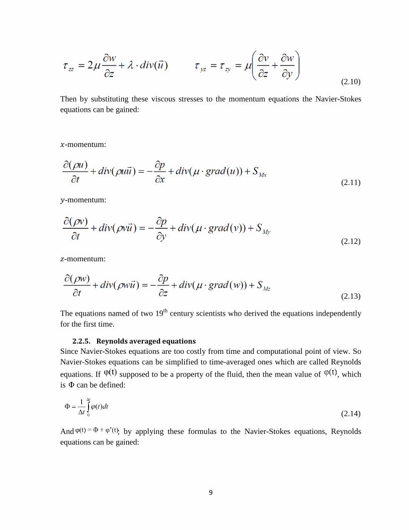
Figure 19: Air velocity contour with mean inlet air velocity of 18.4 m/s

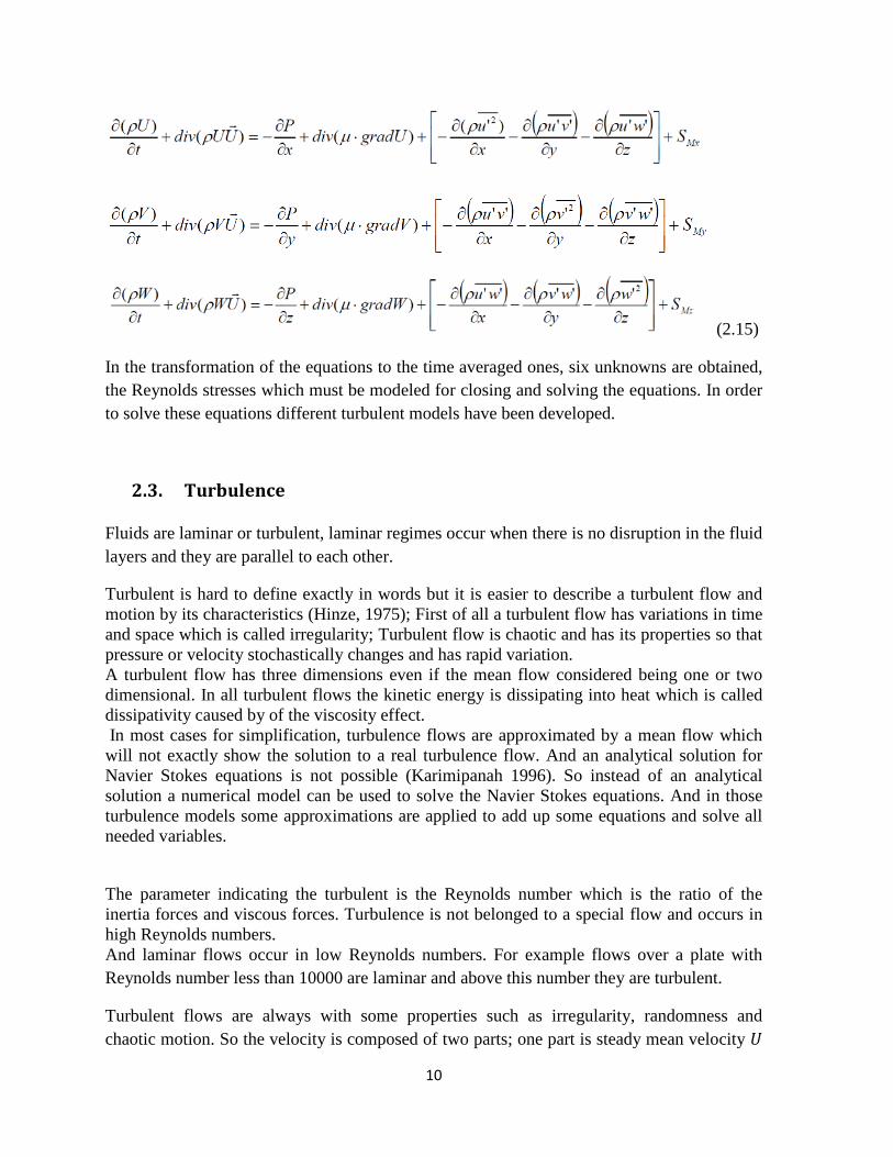
Figure 20: Air velocity contour with mean inlet air velocity of 20.7 m/s

41

Figure 21: Air velocity contour with mean inlet air velocity of 23.9 m/s

As it is shown in the figures (19-21), the velocity contours for different air velocities through the duct, follow the same pattern but with different scales. The air flow jet reaches higher levels and can go further in the duct as the velocity increases. It is also clear in the zoomed part of the figures that the maximum velocity occurs in the region where the area decreases; i.e. due to continuity and conservation of mass since the mass flow is the same and air is considered incompressible (due to the low velocity), so smaller the area, bigger the velocity will be i.e. close to first material outlet.

It is also interesting to see the effect of the main air flow stream after the first step in which it acts like a wall for the small 5m/s air jet (coming from the second material outlet); the small air jet impacts with the main flow stream and attaches to that and then it continues to flow with the main stream and due to the air flow entrainment some vortices occur close to the lower wall of the duct after the step. The small air flow attachment to the main flow stream is also due to Coanda effect which is the tendency of the fluid stream or jet to attach to a nearby surface.

Following contour diagrams depict air dynamic pressure in the duct:

42

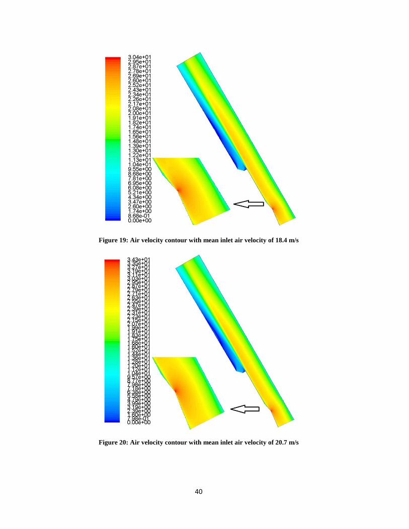
Figure 22: Dynamic pressure contour of the air for the case with air inlet mean flow of 18.4 m/s

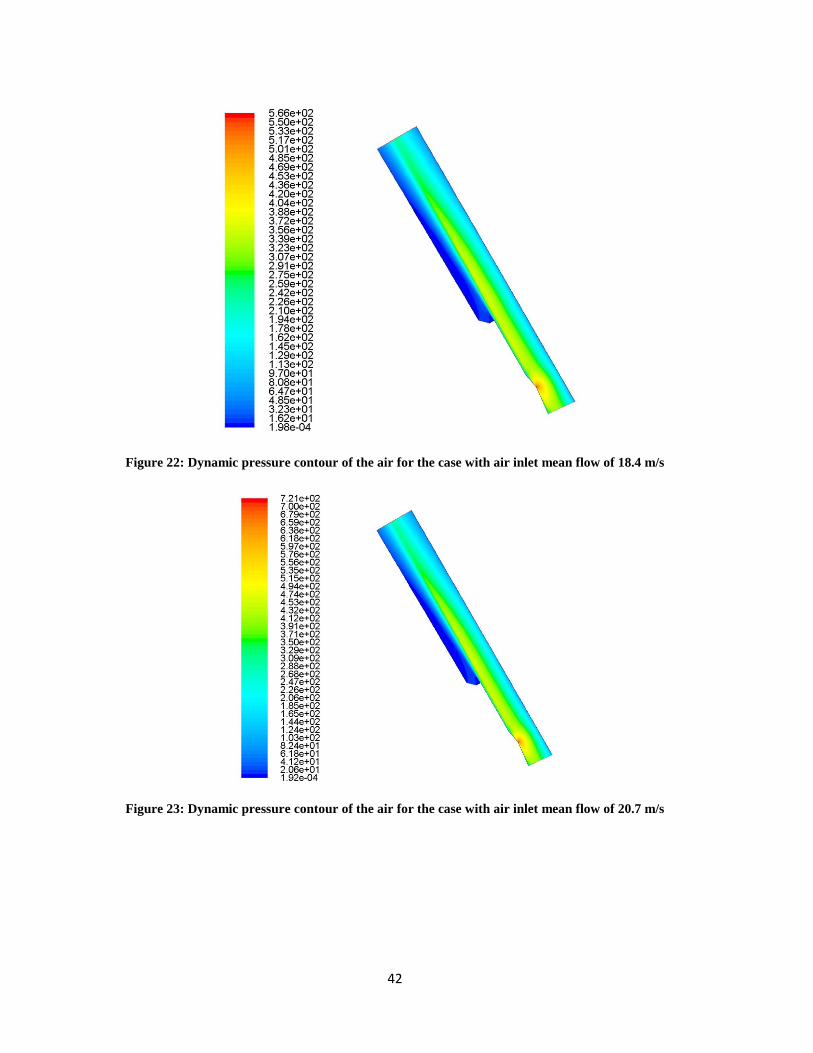
Figure 23: Dynamic pressure contour of the air for the case with air inlet mean flow of 20.7 m/s

43

Figure 24: Dynamic pressure contour of the air for the case with air inlet mean flow of 23.9 m/s

Contour diagrams of the dynamic pressure follow the velocity pattern, since it is the pressure due to the velocity. The maximum dynamic pressure occurs near the first material inlet where the area decreases and velocity increases. After the first step and above the duct the air flow loses its momentum and dynamic pressure decreases as well. All three dynamic pressure contours are like each other in pattern but their scale is different by 20-30 %.

Contour diagrams of the air total pressure are depicted as follows:

44

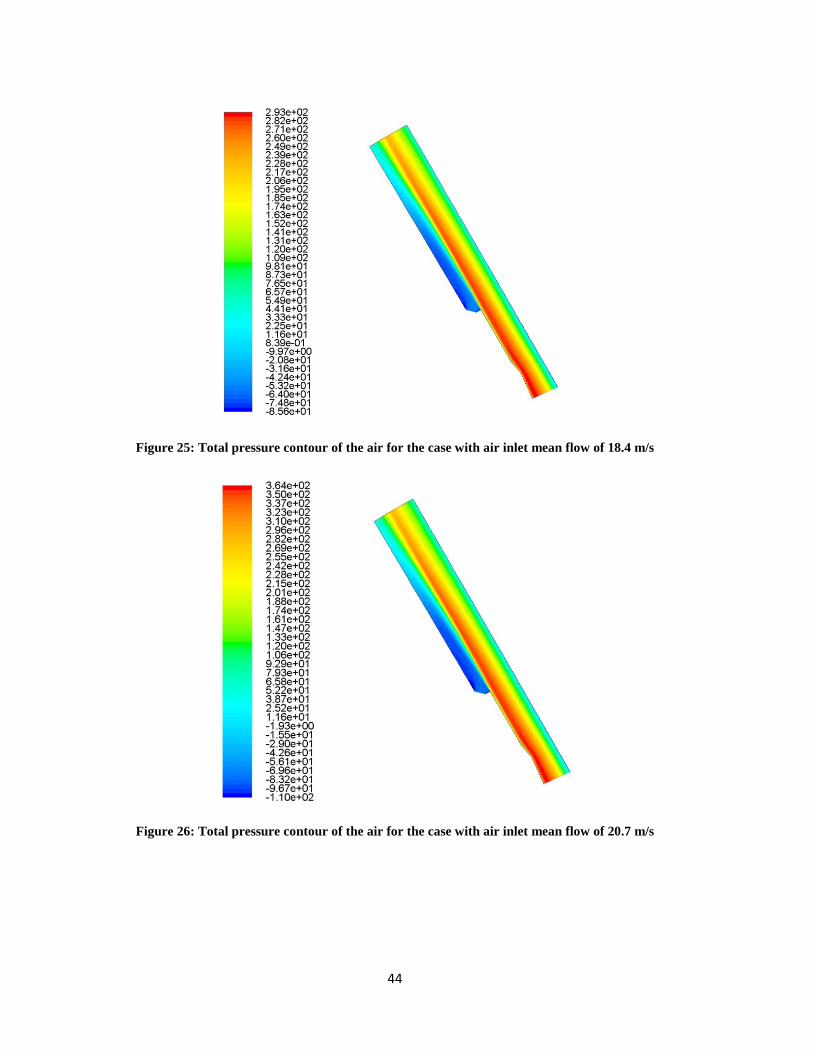
Figure 25: Total pressure contour of the air for the case with air inlet mean flow of 18.4 m/s

Figure 26: Total pressure contour of the air for the case with air inlet mean flow of 20.7 m/s

45

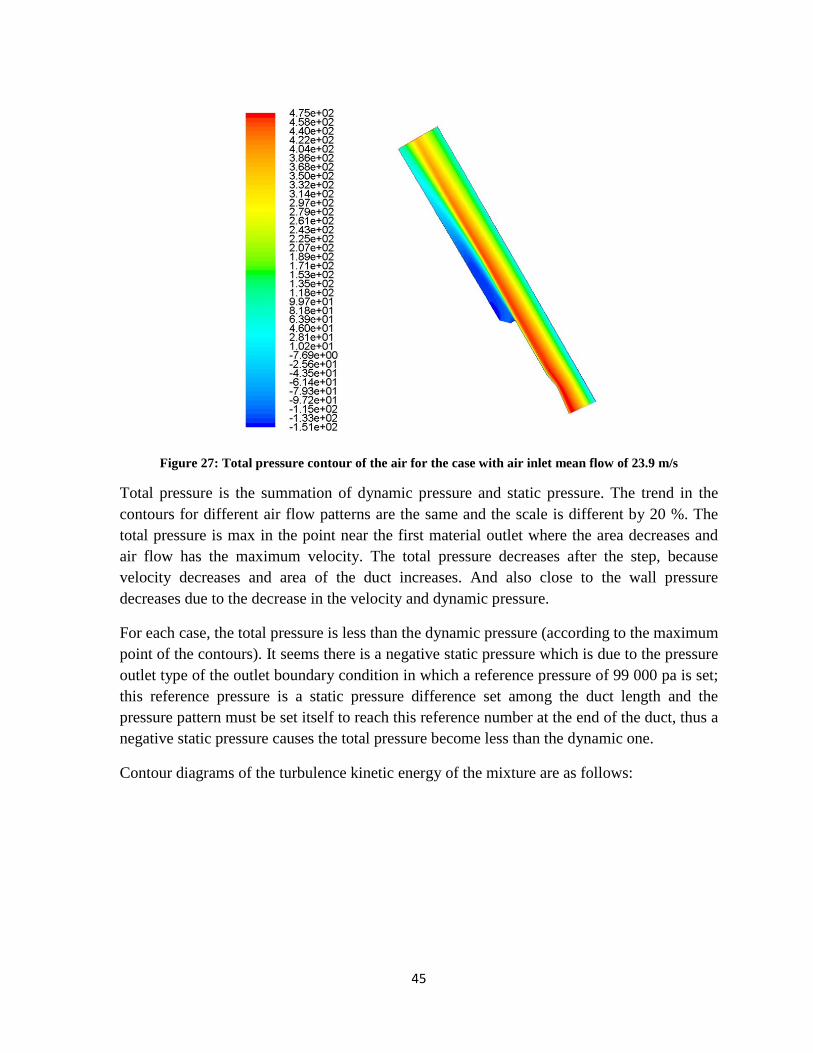
Figure 27: Total pressure contour of the air for the case with air inlet mean flow of 23.9 m/s

Total pressure is the summation of dynamic pressure and static pressure. The trend in the contours for different air flow patterns are the same and the scale is different by 20 %. The total pressure is max in the point near the first material outlet where the area decreases and air flow has the maximum velocity. The total pressure decreases after the step, because velocity decreases and area of the duct increases. And also close to the wall pressure decreases due to the decrease in the velocity and dynamic pressure.

For each case, the total pressure is less than the dynamic pressure (according to the maximum point of the contours). It seems there is a negative static pressure which is due to the pressure outlet type of the outlet boundary condition in which a reference pressure of 99 000 pa is set; this reference pressure is a static pressure difference set among the duct length and the pressure pattern must be set itself to reach this reference number at the end of the duct, thus a negative static pressure causes the total pressure become less than the dynamic one.

Contour diagrams of the turbulence kinetic energy of the mixture are as follows:

46

Figure 28: Turbulence kinetic energy contour for the case with air inlet mean velocity of 18.4 m/s

Figure 29: Turbulence kinetic energy contour for the case with air inlet mean velocity of 20.7 m/s

47

Figure 30: Turbulence kinetic energy contour for the case with air inlet mean velocity of 23.7 m/s

Here vector diagrams of the air velocity and the vortices after the step are shown and the area after the step is zoomed to have a better visualization.

Figure 31: Vector diagram of the air velocity and vortices in the air flow with inlet mean velocity of 18.4 m/s

48

Figure 32: Vector diagram of the air velocity and vortices in the air flow with inlet mean velocity of 20.7 m/s

Figure 33: Vector diagram of the air velocity and vortices in the air flow with inlet mean velocity of 23.9 m/s

49

From figures (28-30) it can be seen that the turbulence kinetic energy is high in the areas after the step (second material outlet), where there are some vortices and by that turbulence increases. It is also interesting to see that just after the second material outlet turbulence does not increase so much, and it is due to the small air jet coming out of second material outlet, which prevents from making intense vortices just after the step and make the flow more laminar and it is clear in the vector figures (31-33) of the area after the step. The turbulence in the region after the step without the small air jet is so high that the cases run without the small jet in the second material outlet had problem with convergence.

4.2.1. Particle velocity tracks The method used in CFD simulations of the cases in this project was one way coupling and as it was discussed in introduction, in this method, particles do not affect the flow pattern and it is just the air which influences the particle flow pattern. So in the study of the effect of particle density and restitution coefficient, the air flow diagrams are the same as before and will not change.

Thus in the following diagrams only the particles traces (tracks) are depicted according to the diameter size of the particles.

Figure 34: Particle velocity tracks for the case with mean inlet air velocity of 18.4 m/s

50

All cases of figures (34-36) have the particle intensity of 2650 kg/m3 and normal particle-wall restitution coefficient of 0.8. It is clear that in case with mean inlet air velocity of 18.4 m/s, heavy particles fall in the first material outlet. And the finer ones exit through the duct outlet. And it is interesting to see the behavior of the 4 mm particles, when the air momentum cannot push them out of the duct, and just before the duct outlet they come back and finally fall in the second material outlet. In this case the light particles of 1 - 3 mm diameter are pushed out of the duct and the heavy particles of diameter between 6 and 8 mm fall down in the first material outlet (figure 34).

Figure 35: The base case; Particle velocity tracks for the case with mean inlet air velocity of 20.7 m/s

In case with mean inlet air velocity of 20.7 m/s, all particles are pushed out from the main outlet except the 7 mm and 8mm particles; 8mm particles are so heavy that directly go to the first material outlet and 7mm particles are not light enough to be taken out from the main outlet and they collide and bounce on the lower wall after the step. 7mm particles have a lot of bouncing and finally fall into the second material outlet.

51

Figure 36: Particle velocity tracks for the case with mean inlet air velocity of 23.9 m/s

In case with mean inlet air velocity of 23.9 m/s, the air flow momentum is so high that all particles are pushed out from the duct and no particle enter the first or second material outlet. And it is good to notice that due to the high momentum of the air flow, lighter particles of 1-6 mm tend to follow the main stream after the collision or in case of 1 mm particles even without collision.

52

Figure 37: Particle velocity tracks of cases with different mean inlet air velocity

In the figure (37) the upper part of the duct is zoomed to see the particle bouncing and collision on the wall. In these cases the normal wall-particle restitution coefficient is 0.8 and the tangential one is 1. It can be seen that the air flow momentum affect the flow pattern just before collision and in the collision particles behave in the same condition due to the same restitution coefficients that all cases have, i.e. there is the same ratio between the relative velocities before and after impact.

4.3. Effect of particle density

Two more particle densities are simulated and the particle-wall collisions are investigated. In addition to the base case particle density (2650 kg/m3), particle densities of 1500 and 3000 kg/m3 are studied.

In the following diagrams the particles traces (tracks) are depicted according to the diameter size of the particles.

53

Figure 38: Particle velocity tracks for the case with particle density of 1500 kg/m3

As it can be seen as particles become heavier, their bouncing in the collision with the wall increases. It can be seen in figure (38) that all particles with density of 1500 kg/m3 are pushed out of the duct by the air flow with mean inlet velocity of 20.7 m/s, these particle are so light that the 1 and 2mm diameter sizes of them even do not collide with the wall and directly exit the duct, of course because of gravity, they tend to come down but any way they cannot reach the wall and make any collision with the wall.

In case of particle density of 2650 kg/m3 which is the base case, Figure (35), particles with diameter size of 7 mm bounce and fall into the second material outlet; the heaviest particles of 8 mm size fall down directly into the first material outlet and the rest are forced to go out of the duct through the main outlet.

54

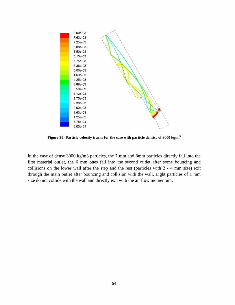
Figure 39: Particle velocity tracks for the case with particle density of 3000 kg/m3

In the case of dense 3000 kg/m3 particles, the 7 mm and 8mm particles directly fall into the first material outlet, the 6 mm ones fall into the second outlet after some bouncing and collisions on the lower wall after the step and the rest (particles with 2 - 4 mm size) exit through the main outlet after bouncing and collision with the wall. Light particles of 1 mm size do not collide with the wall and directly exit with the air flow momentum.

55

Figure 40: Particle velocity tracks for cases with different particle densities

In figure (40) it can be seen in the zoomed upper side of the duct that particle flows with 1500 kg/m3 have smoother flow pattern and tend to follow the air flow stream. And it seems that the air flow momentum is not enough to push 7 mm and 6 mm particles in the cases with particle density of 2650 kg/m3 and 3000 kg/m3 respectively.

4.4. Effect of restitution coefficient

Here are the results for three different normal wall-particle restitution coefficients of 0.5, 0.8 (the base case) and 0.9; and particles traces (tracks) are depicted according to the diameter size of the particles.

56

Figure 41: Particle velocity tracks for the case with normal wall-particle restitution coefficient of 0.5

The only change is in the normal restitution coefficient. As the base normal particle-wall restitution coefficient of 0.8 was discussed, the bouncing is more for the 7 mm particles since they are not light enough to be pushed up in the duct (figure 35). For the normal restitution coefficient of 0.5, particles do not tend to reflect sharply into the domain and they are closer to the wall; it seems that normal restitution coefficient of 0.5 is not so realistic since particles do not bounce and they rather prefer to stick to the wall especially for the particle sizes of 6mm and 7mm which just slide on the wall and exit from the second material outlet.

57

Figure 42: Particle velocity tracks for the case with normal wall-particle restitution coefficient of 0.9

In the case with normal restitution coefficient of 0.9, particles reflect sharper after the collision with the wall. Particles with size of 7 mm go further up in the duct but still exit from the second material outlet with more bouncing; since they are not light enough for the air flow and air flow momentum cannot push them up in the duct. Also it is clear that the more normal restitution coefficients, more far away are the particles from the walls.

It is also interesting to mention that the 8 mm size particles which directly exit from the first material outlet, still do the same with changing the restitution coefficient since they have no collision with wall and changing the restitution coefficient does not affect them.

58

Figure 43: Particle velocity tracks for the cases with different normal wall-particle restitution coefficient

In the upper side zoomed figure (43) the bouncing and reflection effect of the normal restitution coefficient is more tangible; the more the coefficient, the sharper the reflection is and particles are thrown with more angle into the domain, and later on by the air flow momentum, they pushed forward and exit from the domain or collide again with the wall. In cases with heavy particles and low restitution coefficient, air flow cannot push them forward and they bounce back to the second material outlet.

4.5. More injection

In this case more particle streams from the same size are injected to see the effect of turbulent velocity fluctuations as well as the range of the collisions points; moreover more details about the particles traces (tracks) are shown in the computational domain.

59

Figure 44: Particle velocity tracks for the base case with more iteration

In this case more streams of particles are injected from each point, thus more fluctuations of the flow streams can be seen, as well as a range of collision points for each particle size. This case is the base one with particle density of 2650 kg/m3, air inlet mean velocity of 20.7 m/s and normal restitution coefficient of 0.8. In this case, like the case with one injection, the 8 mm particles go directly into the first material outlet, the 7 mm collide with the lower wall and finally leave the duct through the second material outlet and the rest exit from the main outlet after colliding with the wall.

4.6. The chart for track of particles

Here is the table for the results of the particle tracking in the simulated cases; table below shows that from which outlet each particle size exits and also the number off bouncing for each case is shown.

60

Table 1: Particle distribution according to the exit outlet and number of bouncing

The table shows light particles less than 4 mm diameter size exit from the main outlet, while lighter ones of 1mm have no bouncing and directly exit, 2 and 3mm ones have one collision with the wall. 4mm particles have at least one and even up to six times of bouncing. 6 and 7 mm particles behavior depend strongly on the simulation case. And finally 8 mm size particle are the heaviest ones and mostly directly exit from the first material outlet, and in cases they have collision with the wall, they exit from the main outlet.

exit outlet Number of bouncing exit outlet Number of bouncing exit outlet Number of bouncing1 The base case main outlet 0 main outlet 1 main outlet 12 Mean inlet Vair 18.4 main outlet 0 main outlet 1 main outlet 13 Mean inlet Vair 23.9 main outlet 0 main outlet 1 main outlet 14 Partile density 1500 kg/m3 main outlet 0 main outlet 0 main outlet 15 Partile density 3000 kg/m3 main outlet 0 main outlet 1 main outlet 16 Restitution coefficient 0.5 main outlet 0 main outlet 1 main outlet 17 Restitution coefficient 0.9 main outlet 0 main outlet 1 main outlet 1

Patricle diamter (mm) 21 3

exit outletNumber of bouncing

exit outletNumber of bouncing

exit outletNumber

of bouncing

exit outletNumber

of bouncing

1 main outlet 2 main outlet 2 material outlet 2 3 material outlet 1 02 material outlet 2 6 material outlet 1 0 material outlet 1 0 material outlet 1 03 main outlet 1 main outlet 1 main outlet 2 main outlet 34 main outlet 1 main outlet 1 main outlet 1 main outlet 25 main outlet 2 material outlet 2 4 material outlet 1 0 material outlet 1 06 main outlet 2 material outlet 2 4 material outlet 2 4 material outlet 1 07 main outlet 2 main outlet 2 material outlet 2 5 material outlet 1 0

Patricle diamter

(mm)

84 6 7

61

5. Conclusions

The particle flow pattern in solid-gas multiphase flows is so complicated and strongly depends on the so many parameters, such as air flow velocity, particle density and normal restitution coefficient; there are other parameters which kept constant in this thesis but can be important on the flow pattern; such as tangential restitution coefficient, particle velocity, mass flow rate of the particle, geometry of the duct and sizes, position of the material outlet, position of the material inlet, air flow pattern.

From the CFD simulation it is observed that changing the air velocity, particle density, and the restitution coefficient is very effective on the particle flow pattern, and it is important to select the appropriate range according to the application; for normal restitution coefficients it is concluded that a range between 0.8 to 1 is closer to reality and gives better results and at low values like 0.5 particles attach to the wall and slide on that instead of bouncing which happens in reality.

The more the normal restitution coefficient, the sharper the reflection is and particles are reflected back into the computational domain, and later on by the air flow momentum, they may be pushed forward and exit out from the domain or bounce again with the wall. In case with heavy particles and low restitution coefficient, air flow cannot push them forward and they bounce back into the duct.

The position of the inlet and outlets of the air flow and material plays a dominant role in the particle behaviour and air flow turbulence, for example the small air jet at the second material outlet prevent formation of intensive vortices just after the step where the area of the duct increases.

Choosing a right velocity for the industrial applications of solid-gas multiphase flows, depends highly to the density of the particles and this factor plus the duct length determine the needed air flow pattern and velocity to ensure the momentum required to convey the material.

First of all it is suggested that a prototype of the geometry can be made and some experimental data for verification of the CFD simulation results can be gained by measurement.

Although multiphase models are not fully developed, more precise CFD models can be used for going further, such as Eulerian model with Population Balance Model (PBM) which is more accurate, this model is available in ANSYS FLUENT 14.

62

It is also good to mention that a 3D model can predict better results since air can find some ways to go through the particles (in case with a model considering the effect of the particles on the air flow); and the simulation result might be more realistic.

Also two way coupling model can be applied for the simulation to go further since the particles affect the air flow though this model does not consider the particle-particle collisions.

63

References ANSYS Inc., 2009, ANSYS FLUENT 12.0 Theory Guide. [e-book], ANSYS, Inc. Available through: <www.fluentusers.com> [Accessed 8 May 2012]

Bettega, R., Correa,R.G., Freire, J.T., 2009a. Scale-upstudy of spouted beds using computational fluiddynamics. Canadian Journal of Chemical Engineering, 87, pp.193–203.

Bettega, R., da Rosa, C.A., Correa, R.G., etal., 2009b. Fluid dynamic study of a semi cylindrical spouted bed: evaluation of the shear stress effects in the flat wall region using computational fluid dynamics. Industrial & Engineering Chemistry Research, 48, 11181–11188.

Bettega, R., De Almeida, A.R.F., Correa,R.G., etal., 2009c. CFD modeling of a semi-cylindrical spouted bed: numerical simulation and experimental verification. Canadian Journal of Chemical Engineering, 87, pp.177–184.

Brennen, Christopher, E,. 2005. Fundamentals of multiphase flow. Cambridge University Press.

Cammarata, L., Lettieri, P., Micale, G.D.M., Colman, D., 2003. 2d and 3d CFD simulations of bubbling fluidized beds using Eulerian–Eulerian models. Int.J.Chem. ReactorEng., pp.48–55.

Crowe, C.T., Sommerfeld, M. and Tsuji, Y. 1998. Multiphase Flows with Droplets and Particles. CRC Press, Boca Raton, FL.

Elghobashi, S.E. and Truesdell, G.C. 1993. On the two-way interaction between homogeneous turbulence and dispersed solid particles. I: Turbulence modification. Physics Fluids, A5, 1790-1801.

Ferziger, J.H., 1983. Higher-Level simulations of Turbulent Flows. In Essers J.A. (ed), Computational Methods for Turbulent, Transonic and Viscous Flows, Hemisphere, New York,

Fessler, J.R. Kulick, J.D. and Eaton, J.K. 1994. Preferential concentration of heavy particles in a turbulent channel flow. Physics Fluids, 6, 3742-3749.

Fu, J., Adams, M., Reynolds, G., Salman, A., Hounslow M., 2004. Impact deformation and rebound of wet granules. Powder Technology, 25 February,140, pp. 248-257.

Gidaspow, D., Bezburuah, R., Ding, J., 1992. Hydrodynamics of circulating fluidized beds. KineticTheoryApproach, FluidizationVII. In: Proceedings of the Seventh Engineering Foundation Conference on Fluidization, pp.75–82.

64

Gore, R.A. and Crowe, C.T. 1989. The effect of particle size on modulating turbulent intensity. International Journal of Multiphase Flow, 15, 279-285.

Hetsroni, G. 1989. Particles-turbulence interaction. International Journal of Multiphase Flow, 15,735.

Hinze, J., 1975. Turbulence. McGraw-Hill, USA.

Hoomans, B.P.B., Kuipers, Briels, J.A.M., W.J., van Swaaij, W.P.M., 1996. Discrete particle simulation of bubble and slug formation in a two-dimensional gas-fluidised bed: A hard-sphere approach. Chemical Engineering Science, 51, Issue 1, January, pp. 99-118.

Johnson, P.C., Jackson, R., 1987. Frictional–collisional constitutive relations for granular materials, with application to plane shearing. Journal of Fluid Mechanics, 176, pp.67–93.

Karimipanah, T., 1996. Turbulent jets in confined spaces. Ph.D. thesis, Royal Institute of Technology, Sweden.

Kenning, V.M. and Crowe, C.T., 1997. On the effect of particles on carrier phase turbulence in gas-particle flows. International Journal of Multiphase Flow, 23, 403-408.

Lan, X., Chunming Xu, Jinsen Gao, Muthanna Al-Dahhan, 2011. Influence of solid-phase wall boundary condition on CFD simulation of spouted beds, Chemical Engineering Science, 69, pp.419-430.

Li, Y., 1994. Mathematical Modeling of Flow and Heat Transfer in Buildings. A Review. Computational Aerodynamics in Buildings: Report1, CSIRO, Hightett, Vic., Australia.

Link, J.M., Godlieb, W., Deen, N.G., Kuipers, J.A.M, 2007. Discrete element study of granulation in a spout-fluidized bed. Chemical Engineering Science, 62, pp. 195-207.

Longman group Ltd.

Mörl. L., S. Heinrich and M. Peglow,. 2007. Fluidized Bed Spray Granulation. Granulation, Handbook of Powder Technology, Vol. 11, Elsevier Science, pp. 21-88.

Olsson, M., 1995. Large Edyy Simulations of Spatially Developing Jets. Thesis of Licentiate Engineering, Department of Mechanics, Royal Institute of Technology, Stockholm

Pan. Y. and Banerjee, S. 1997. Numerical investigation of the effects of large particles in wall-turbulence. Physics Fluids, 9, 3786-3807.

Parathasarathy, R.N. and Faeth, G.M. 1987. Structure of the particle-laden turbulent water jets in still water. International Journal of Multiphase Flow, 13, 699-716

Paris, A.D. and Eaton, J.K. 2001. Turbulence attenuation in a particle laden channel flow. Mechanical Engineering Department, Stanford University Report.

65

Passos, M.L., Mujumdar, A.S., 2000. Effect of cohesive forces on fluidized and spouted beds of wet particles, Powder Technology, Volume 110, Issue 3, 12 June, Pages 222-238.

Peirano, E., Delloume, V., Leckner, B., 2001. Two or three dimensional simulations of turbulent gas–solid flows applied to fluidization. Chemical Engineering Science, 56, 4787–4799.

Squires, K.D. and Eaton, J.K. 1990. Particle response and turbulence modification in isotropic turbulence. Physics Fluids, A2, 1191-1203.

Tabakoff, W., and Wakeman, T., 1982. Measured particle rebound characteristics useful for erosion prediction. ASME paper, 82-GT-170.

van Buijtenen, M. S., Deen, N. G., Heinrich, S., Antonyuk, S. and Kuipers, J. A. M., 2009. Discrete Particle Simulation Study on the Influence of the Restitution Coefficient on Spout Fluidized-Bed Dynamics. Chemical Engineering Technology, 32, pp.454–462.

Versteeg, H.K. and Malalasekera, W., 1995. An introduction to Computational Fluid Dynamics.

Vieira, M.G.A., Rocha, S.C.S., 2004. Influence of the liquid saturation degree on the fluid dynamics of a spouted-bed coater. Chemical Engineering and Processing: Process Intensification, Volume 43, Issue 10, October, pp. 1275-1280.

Wang, X., Jin, B., Zhong, W., etal., 2009. Modeling on the hydrodynamics of a high-flux circulating fluidized bed with Geldart Group A particles by kinetic theory of granular flow. Energy Fuels, 24, pp. 1242–1259.

Yuan, Z. and Michaelides, E.E. 1992. Turbulence modulation in particulate flows-a theoretical approach. International Journal of Multiphase Flow, 18, 779-785.