Embed Size (px)
Citation preview

Intelligent Target Selection for Direct
Marketing
Sjoerd van Geloven
25 April 2002

ii

Preface
This report is the description of the thesis project "Intelligent Target Selection
in Direct Marketing", the �nal project of the Electrical Engineering curriculum
given at the Faculty Information Technology and Systems (ITS) at Delft Uni-
versity of Technology (DUT).
This thesis originated of a mutual interest of the Control Laboratory of the
ITS faculty and the Department of Computer Science of the Economics Faculty
of the Erasmus University in Rotterdam in the use of Arti�cial Intelligence (AI)
in Direct Marketing.
I would like to thank Robert van Amerongen and Robert Babuska, from the
Control group, for giving me the opportunity to work on this interesting project
that is not a typical graduation project for Electrical Engineering students. Fur-
thermore, I am grateful to both for their critical comments and the latter for
his support during the implementation phase.
From the Erasmus University, I would like to thank Willem-Max van der Bergh,
Jan van den Berg and Uzay Kaymak for their guidance and support through
this project. Especially the latter, who provided the project description and
provided me with both a lot of insight information on the subject of target se-
lection and the fuzzy algorithm implementation.
Sjoerd van Geloven
25 April 2002
iii

iv PREFACE

List of Tables
2.1 Di�erent types of variables . . . . . . . . . . . . . . . . . . . . . . 9
3.1 Spector and Mazzeo data . . . . . . . . . . . . . . . . . . . . . . 19
3.2 CoeÆcients and t-ratios compared . . . . . . . . . . . . . . . . . 20
4.1 Example scatter matrix . . . . . . . . . . . . . . . . . . . . . . . 33
5.1 CPM values for linear regression with all features . . . . . . . . . 45
5.2 Features with large correlation to Caravan policies owners . . . . 47
5.3 CPM values for linear regression with correlation features . . . . 48
5.4 Features selected by logit as signi�cant . . . . . . . . . . . . . . . 48
5.5 CPM values for logit . . . . . . . . . . . . . . . . . . . . . . . . . 49
5.6 CPM values for the NNs . . . . . . . . . . . . . . . . . . . . . . . 50
5.7 CPM values for the fuzzy modeling technique . . . . . . . . . . . 51
5.8 Weight factors for example 1 . . . . . . . . . . . . . . . . . . . . 53
5.9 Numerical performance measures example 1 . . . . . . . . . . . . 54
5.10 Weight factors for example 2 . . . . . . . . . . . . . . . . . . . . 55
5.11 Numerical performance measures example 2 . . . . . . . . . . . . 55
A.1 Listing of the attributes 1 to 43 . . . . . . . . . . . . . . . . . . . 62
A.2 Listing of the attributes 44 to 86 . . . . . . . . . . . . . . . . . . 63
A.3 Category L0 . . . . . . . . . . . . . . . . . . . . . . . . . . . . . . 64
A.4 Category L1 . . . . . . . . . . . . . . . . . . . . . . . . . . . . . . 65
A.5 Category L2 . . . . . . . . . . . . . . . . . . . . . . . . . . . . . . 65
A.6 Category L3 . . . . . . . . . . . . . . . . . . . . . . . . . . . . . . 65
A.7 Category L4 . . . . . . . . . . . . . . . . . . . . . . . . . . . . . . 65
v

vi LIST OF TABLES

List of Figures
2.1 Gain chart explanation . . . . . . . . . . . . . . . . . . . . . . . . 13
3.1 Activation functions . . . . . . . . . . . . . . . . . . . . . . . . . 26
4.1 Correlations of feature pairs 1 and 5, 30 and 31, 35 and 36 . . . . 35
4.2 Flow chart of data sets and performance measures . . . . . . . . 41
4.3 Methodology . . . . . . . . . . . . . . . . . . . . . . . . . . . . . 42
5.1 Gain chart for linear regression using all features . . . . . . . . . 46
5.2 Gain chart for logit with 7 best logit features . . . . . . . . . . . 49
5.3 Gain chart for Chaid . . . . . . . . . . . . . . . . . . . . . . . . . 50
5.4 Gain chart for neural network I . . . . . . . . . . . . . . . . . . . 51
5.5 Gain chart for fuzzy model . . . . . . . . . . . . . . . . . . . . . 52
5.6 Gain charts example 1 . . . . . . . . . . . . . . . . . . . . . . . . 54
5.7 Gain charts example 2 . . . . . . . . . . . . . . . . . . . . . . . . 56
5.8 Results participants of CoIL 2000 . . . . . . . . . . . . . . . . . . 57
vii

viii LIST OF FIGURES

Contents
Preface iii
1 Introduction 1
2 Target Selection in Direct Marketing 3
2.1 Direct Marketing . . . . . . . . . . . . . . . . . . . . . . . . . . . 3
2.2 Target Selection and KDD . . . . . . . . . . . . . . . . . . . . . . 6
2.2.1 Preparing . . . . . . . . . . . . . . . . . . . . . . . . . . . 7
2.2.2 Data mining . . . . . . . . . . . . . . . . . . . . . . . . . 10
2.2.3 Interpretation . . . . . . . . . . . . . . . . . . . . . . . . . 11
2.3 Gain charts . . . . . . . . . . . . . . . . . . . . . . . . . . . . . . 12
3 Mining algorithms 15
3.1 Linear regression . . . . . . . . . . . . . . . . . . . . . . . . . . . 16
3.1.1 Linear regression assumptions . . . . . . . . . . . . . . . . 17
3.1.2 Feature selection and correlation . . . . . . . . . . . . . . 17
3.1.3 Strengths and weaknesses . . . . . . . . . . . . . . . . . . 18
3.2 Logit . . . . . . . . . . . . . . . . . . . . . . . . . . . . . . . . . . 18
3.2.1 Implementation and veri�cation . . . . . . . . . . . . . . 19
3.2.2 Scaling . . . . . . . . . . . . . . . . . . . . . . . . . . . . 20
3.2.3 Feature selection . . . . . . . . . . . . . . . . . . . . . . . 20
3.2.4 Strengths and weaknesses . . . . . . . . . . . . . . . . . . 21
3.3 Chaid . . . . . . . . . . . . . . . . . . . . . . . . . . . . . . . . . 21
3.3.1 The chi square test . . . . . . . . . . . . . . . . . . . . . . 23
3.3.2 Signi�cance of the predictors . . . . . . . . . . . . . . . . 23
3.3.3 Implementation . . . . . . . . . . . . . . . . . . . . . . . . 24
3.3.4 Strengths and weaknesses . . . . . . . . . . . . . . . . . . 24
3.4 Neural Networks . . . . . . . . . . . . . . . . . . . . . . . . . . . 25
3.4.1 The feedforward-backpropagation NN . . . . . . . . . . . 25
3.4.2 Implementation . . . . . . . . . . . . . . . . . . . . . . . . 27
3.4.3 Strengths and weaknesses . . . . . . . . . . . . . . . . . . 27
3.5 Fuzzy modeling . . . . . . . . . . . . . . . . . . . . . . . . . . . . 28
3.5.1 Feature selection . . . . . . . . . . . . . . . . . . . . . . . 28
3.5.2 Target selection . . . . . . . . . . . . . . . . . . . . . . . . 29
3.5.3 Strengths and weaknesses . . . . . . . . . . . . . . . . . . 29
3.6 Summary of target selection algorithms . . . . . . . . . . . . . . 29
ix
x CONTENTS
4 Methodology 31
4.1 Data set and direct marketing . . . . . . . . . . . . . . . . . . . . 31
4.1.1 Original TIC assignment . . . . . . . . . . . . . . . . . . . 31
4.1.2 The direct marketing questions . . . . . . . . . . . . . . . 32
4.2 Performance measures . . . . . . . . . . . . . . . . . . . . . . . . 33
4.2.1 Numerical Gain Chart Value . . . . . . . . . . . . . . . . 34
4.2.2 CoIL Performance Measure . . . . . . . . . . . . . . . . . 34
4.3 Target Selection by KDD . . . . . . . . . . . . . . . . . . . . . . 34
4.3.1 Correlation between the Features . . . . . . . . . . . . . . 35
4.3.2 Con icting rows . . . . . . . . . . . . . . . . . . . . . . . 36
4.3.3 Scaling . . . . . . . . . . . . . . . . . . . . . . . . . . . . 37
4.3.4 Feature selection . . . . . . . . . . . . . . . . . . . . . . . 37
4.3.5 Di�erent types of variables . . . . . . . . . . . . . . . . . 37
4.3.6 Combining the algorithms . . . . . . . . . . . . . . . . . . 38
4.3.7 Test structure . . . . . . . . . . . . . . . . . . . . . . . . . 40
5 Results 45
5.1 Stand-alone algorithms . . . . . . . . . . . . . . . . . . . . . . . . 45
5.2 Combing the algorithms . . . . . . . . . . . . . . . . . . . . . . . 53
5.3 Comparison to previous results and discussion . . . . . . . . . . . 55
6 Conclusions and Recommendations 59
A Tables of the features and datasets 61

Chapter 1
Introduction
Direct marketing is the process of approaching customers with the intention to
sell products or services. Because the typical response is low, it is worthwhile to
know which customers are interested in the o�er in mind. In this way, resources
can be directed to the pro�table customers. It is, however, very diÆcult to
predict in advance, which persons are interested in a speci�c product or service.
This problem is known as "target selection" in direct marketing, in which the
targets are the prospects who will respond.
Most companies have a lot of information about their customers. The purchase
history and zip code information are usually present in a client database. Zip
code information contains the typical characteristics of an individual living in
a certain zip code district. A characteristic, e.g. age, of clients stored in such a
database is called a variable, attribute or feature. These features can be used
to describe customers which hopefully results in a certain likelihood of response.
A general approach to tackle the diÆculties in predicting the response of prospects
is Knowledge Discovery in Data. For the part in this process dealing with the
mining of clients resulting in a certain likelihood of response, several algorithms
have been used over the years. The relation between the attributes and the vari-
able describing the response is expected to be non-linear, because of the fact
that humans tend to base their decisions on both knowledge and emotion. We
do not have the availability of these factors, but we do have knowledge of some
characteristics of the prospects. We hope that the features used in a certain
con�guration are good predictors but also know that human decision making
does not always depend on rational thinking. So, the assumption is that the
relationship between the features and the target variable has a non linear char-
acter. The degree of this non-linearity is not known. This is the reason why
many target selection algorithms with various complexity structures are used
during the last decades. Five of them, increasing in complexity, are subject of
study in this thesis.
Another goal of this project is to investigate whether the algorithms (three
statistical ones and two algorithms based on arti�cial intelligence) used for the
purpose of target selection in direct marketing could help each other in order to
capture the assumed high complexity and ultimately obtain better results. More
speci�cally, can the strength of an algorithm overcome a weakness of another?
1

2 CHAPTER 1. INTRODUCTION
For example, can the feature subset denoted as signi�cant by one algorithm
prove better results for a second? The intention is to build a system which is
more intelligent than a stand-alone algorithm in order to capture assumed high
non-linearity but still can act as autonomously as possible. This last demand is
added because the intervention of domain experts is time consuming and expen-
sive. The underlying thought for this operation is that every gain in targeting
the most valuable customers directly results in extra revenue, and eventually
increases pro�ts.
Before the questions above can be answered, the algorithms suited for target
selection have to be studied and compared. Another interesting question is
whether di�erent types of variables (binary, categorical, continuous or other)
and scaling (transforming the feature values) have impact on target selection.
These e�ects are studied for each algorithm or con�guration.
So, the main goal of this thesis is to investigate which con�guration of one
or more algorithms performs best for the purpose of target selection in direct
marketing. Furthermore, the scaling and di�erent type of variable treatments
of this con�guration are explored.
The outline of this thesis is as follows: in chapter 2 the application domain
of direct marketing is further explored and the approach of target selection by
means of Knowledge Discovery in Data explained. Chapter 3 describes the �ve
algorithms used for target selection in this thesis by their mathematical back-
ground. Not all algorithms can be applied in a straight-forward way: some
algorithm speci�c variables need to be set. These parameter choices and ad-
ditional implementation issues are also covered in chapter 3. In chapter 4 the
search for complexity �t starts. After introducing some performance measures
used for comparing the di�erent con�gurations, all algorithms are optimized
for the purpose of target selection. The methodology is explained by a real-
life direct marketing target selection problem. This data set is introduced and
suggestions for optimal target selection are given for this example. The chap-
ter ends with fertile combinations of algorithms: the con�gurations which can
cope with the highest complexity. Results of the stand-alone algorithms and the
combinations on this real-life data set are presented in chapter 5, together with
a comparison to previous obtained results on this data set. Finally, in chapter
6 conclusions are drawn and recommendations are made for further research.
Chapter 2
Target Selection in Direct
Marketing
"A general rule of thumb in marketing is that approximately 20 percent of a
company's customers account for about 80 percent of its business." ... "It is not
worthwhile for a company to o�er generous promotions to the other 80 percent.
The more these loyal customers are retained, the more data can be gathered
about them." [1]
From this fragment it may be concluded that it is very important to know which
customers would be interested in certain o�ers.
This chapter tries to give insight in the way target selection in direct marketing
can be applied and �rst of all, what direct marketing is. The application domain,
direct marketing, is explored in section 2.1. Section 2.2 provides an overview
of the Knowledge Discovery in Data cycle, a general method very well suitable
for target selection. Finally, in section 2.3 gain charts are explained; the graphs
used in this thesis to compare results.
2.1 Direct Marketing
Direct marketing is a powerful tool for companies to increase pro�t, especially
when one knows his customers well. A de�nition of direct marketing is: "Direct
marketing is the science of arresting the human intelligence long enough to take
money o� it" [3]. This sounds cynical, but true. However, a formal de�nition
needs more than a laugh. The Direct Marketing Association, the industry's
oÆcial trade association, de�nes direct marketing as "an interactive system of
marketing which uses one or more advertising media to e�ect a measurable re-
sponse or transaction at any location." In a general marketing activity, there are
three matters to be analyzed: the customers, the competitors and the company
marketing the product. In this thesis, the focus is on the customers. How can
the most valuable customers or prospects be targeted?
The advantage of direct marketing compared to other marketing activities is
that it seeks a direct response from pre-identi�ed prospects. It allows compa-
nies to direct their energies toward those individuals who are most likely to
respond. This selectivity is necessary to enable the use of high cost { high
3

4 CHAPTER 2. TARGET SELECTION IN DIRECT MARKETING
impact marketing programs such as personal selling in the business-to-business
environment [4]. A second fundamental characteristic of direct marketing is that
it generates individual response by known customers. This enables companies to
construct detailed customer purchase histories, which tend to be far more useful
than traditional predictors based on geodemographics and psychographics [4].
The growth of direct marketing can be explained by several changes in the
social environment [2] [5]. First of all, the composition of households changed.
Nowadays a large number of women joins the labor force and there are more
double-income households then ever. Secondly a re-evaluation of leisure time
is taking place. Next to this, credit cards o�er convenience and the required
security for payments. Another enabler is the information and communication
technology: high computing power allows computations that never could be
done by humans, larger amounts of data can be stored is and new advertising
media like the Internet, e-mail and WAP (Wireless Application Protocol, used
in Telecommunications for data transport) are introduced. Last but not least
new life styles and consumer values are incorporated in society. Direct market-
ing provides opportunities for identifying, measuring and reaching these groups
as market segments.
Generally, there are two ways to identify those customers who are most likely
to respond to o�erings. Either you have a customer database yourself, or you
acquire a list from, so-called, list brokers. Apart from the list, there are some
other issues to take into account. In direct marketing, �ve questions are often
considered [3]:
1. Who am I trying to reach?
2. What do I want them to do?
3. Why should they do it?
4. Where should I reach them?
5. When should I reach them?
Who? This question corresponds to target selection. At �rst, the target mar-
ket has to be de�ned. To whom does a company want to make an o�er?
Businesses or consumers? Existing customers or new? And the most im-
portant consideration: which prospects? The second question is whether
the company has suÆcient data on the subjects de�ned as target marker
or that extra information is obliged? List brokers sell lists with, for ex-
ample, zip code characteristics. Furthermore, it is obvious that one would
like to address those customers, who are likely to respond. But speci�c
campaign information can still be important because of the fact that the
results of the target selection are not known yet. Demographic issues can
play an important role: for instance if the company sells music records by
mail and they have sponsored a concert, and the target selection gives all
the customers who like the kind of music performed during the concert,
it is not the smartest thing to invite all of them because not every music
fan will travel hundreds of kilometers to see the concert. In this example,
it would have been wise to only include those customers in the database,

2.1. DIRECT MARKETING 5
who live in the surroundings of the location of the concert. This pre-
selection can be seen as a form of feature selection which is dealt with in
section 2.2.1. Now that the customer data base is built, the targets from
this data base can be selected. This corresponds to the question: "Which
customers are the targets of this campaign?" A general approach for the
purpose of target selection (including the selection or building of the data
base) is presented in section 2.2.
What? The proposition one would like to make has to be de�ned here. What is
one selling and how should the recipient of the communication react? One
of the �rst things to decide is whether the response should be one or two-
stage; does one want merely an expression of interest or selling products
or services immediately. One stage is sometimes called mail order, where
as two-stage is referred to as direct mail advertising [2]. Next, the kind of
response has to be determined; �lling in a coupon, picking up the phone
and dialing a (toll-free) number, go to a web-site or in another way. Make
this completely clear, and go through the logistics.
Why? Although an enterprise might address its o�er to the ones that are likely
to respond, an attractive o�er could help them to overcome the last doubt.
This is where the unique selling proposition comes in.
Where? If there is only one address per customer available, there is not much
to choose from. But in the professional market there can be a di�erence
in sending to the oÆce or home address. And in most cases even if the
address of the company is known, it is often not entirely clear which person
to address. This is due to the fact that people rotate in a company and
even switch jobs outside a company. So in some cases it seems that one
can better use a job title rather than a name.
When? Timing is one of the few parameters that can be completely controlled.
Timing can make the di�erence between a successful campaign and one
that fails. One thing to consider is the day of the week. Monday morning
and Friday afternoon are not the best times to pick, for the business
customers. In the consumer market the weekend seems to work, because
most households have full-time responsibilities during the week nowadays.
The author of [2] leaves the "where" part out (a proper list must come up with
the right addresses), combines the "why" and "what" and adds a "how". The
how-question must come up with the most ideal way of communication. Postal
service, e-mail or another communication element. Next to this, the author
of [2] gives a relative importance in generating response. The right person (or
list) is the most important factor, followed by a good o�er and timing. The
communication element has the least signi�cance, which probably is the reason
why the author of [3] has not mentioned this question in the given questionnaire.
As mentioned above, the "who question" corresponds to target selection in
direct marketing: which prospects does one has to target? Target selection can
be carried out following the Knowledge Discovery in Data cycle. What this is
and how to do this are subjects covered in the next section.

6 CHAPTER 2. TARGET SELECTION IN DIRECT MARKETING
2.2 Target Selection and KDD
This section provides an overview of the Knowledge Discovery in Data cycle: a
general method very well suitable for target selection.
The KDD (Knowledge Discovery in Data) process is interactive and iterative,
involving numerous steps with many decisions being made by the user. The
intention, however, is to construct the process as autonomously as possible.
The preparing stage sometimes is referred to as the most important part of
KDD. Results of a test mailing or previous mailings will structure the input
of this stage. A test mailing is a mailing to a small representative part of a
population. If this stage is not treated in a proper way the saying Garbage In
Garbage Out will take over the best intentions. Depending on the nature of
the data an algorithm for the data mining task has to be chosen. Finally the
results in the form of models or rules have to be interpreted. Asking the help
of a domain expert can be of great assistance. In the end the whole KDD cycle
will end in a go or no go decision in case of direct marketing o�ers. So, we �nd
three stages in KDD: preparing, data mining and interpretation.
KDD is made up of nine basic steps [10].
1. Developing an understanding of the application domain. Collect relevant
prior knowledge and identify the customers' goal of the KDD process.
2. Selection: create a target data set.
3. Preprocessing: remove noise as far as possible, decide on strategies for
handling missing values. This step is also called data cleaning.
4. Transformation: data reduction and projection. Find useful features to
represent the data depending on the goal of the task. Use dimensionality
reduction to reduce the e�ective number of variables under consideration.
5. Matching the goals of the KDD process to a particular data mining method.
6. Choosing the data mining algorithm(s).
7. Data mining: searching for patterns of interest in a particular representa-
tional form.
8. Interpretation of patterns found, and possibly return to any of the steps
1-7.
9. Consolidating the discovered knowledge: incorporating this knowledge in
another system for further action. This system can be the use of the
knowledge to predict the pro�table prospects, or just reporting the re-
sults to the interested parties. This step also includes a validation with
previously obtained results.
Preparing is step 2 to 4, data mining can be divided into step 5 to 7. If the �rst
and the last step are left out, the KDD cycle is complete. The KDD process
can involve signi�cant iterations and may contain loops between any two steps.
In the international literature, most e�ort is focused on the actual data mining
step. The other steps are, however, equally important for a successful applica-
tion of KDD in practice.

2.2. TARGET SELECTION AND KDD 7
In the next subsections these three most important stages, preparing, data min-
ing and interpretation will be addressed individually.
2.2.1 Preparing
The preparing stage consists of three steps: selection, preprocessing and trans-
formation.
Selection
Selection in the phrase "target selection" addresses the entire procedure result-
ing in a selection of the prospects who are most likely to respond from a certain
population. The selection of a test population which will act as "train" samples
for the di�erent con�gurations, is meant here. In the case of direct marketing,
the selection will either involve previous mailings or a test mailing. A test mail-
ing must address a representative subgroup of the entire population. This can
be achieved by a random mailing or by addressing a subgroup, which has repre-
sentative characteristics like a student population. Representative means that
the selection has the same characteristics as the whole population, and that the
size is not too small compared to the population (usually a few percent). One
has to keep in mind that domain expertise can be of great help during the whole
KDD cycle. Relatively expensive o�ers can better be not tested on a student
population because of their limited cash.
Preprocessing
In this step cleaning and removal of noise are the basic operations. Data cleans-
ing is the process of ensuring that all values in data set are consistent and
correctly recorded. This de�nition has two important implications. In the pro-
cess of gathering the data one has to make sure that this is done in a proper
way. One has to check and recheck the sources. If the data is put in a database
by data entries, a thorough check is needed in order to eliminate typing errors.
Even if the information in a database is reliable, one has to cope with noise and
missing values.
Starting with the noise, it is diÆcult to give a proper de�nition of noise. Noise
can be slipped in the data by the procedure used to construct the data set.
There can exist large correlations between features, if, for instance, they repre-
sent more or less the same characteristic. Another type of noise is referred to
as "con icting rows", which is the name of the appearance of exactly the same
feature values and di�erent response values. Although an ideal target selection
con�guration should be able to deal with this type of noise, beforehand it is not
clear what the e�ect will be. So in every KDD process, the impact of these two
types of noise has to be estimated and accordingly proper precautions have to
be taken.
In case of missing values, the �rst thing to consider is the trade-o� between
the time spent on modeling missing values and the potential bene�t. There are
several ways to handle missing values in data �elds:
8 CHAPTER 2. TARGET SELECTION IN DIRECT MARKETING
� Remove all the columns or rows in which missing values are located. Ob-
viously, this solution will only work for a very small number of missing
values, a large amount of available data or a large number of responses.
� Assign the average, mean or modal value. This is simple, but can peak
the distribution, which can become a huge problem when the feature plays
an important role in the decision-making process. In case of a lot of
missing values in the crucial attribute, this solution can give the wrong
impressions. Therefore this solution will in general only be useful in case
of a small number of missing values.
� Distribute the data using the probability distribution of the no missing
records. Still relatively easy to apply, but if the assigned variable is im-
portant, errors will occur in the data mining results.
� Segment the data using the distribution of another variable, and assign
segment averages to missing records in each segment. The results of this
operation heavily depend on the correlation between the variables.
� Combine the previous two methods. DiÆcult to implement, and the gain
again depends on the degree of correlation between the attributes.
� Build a classi�cation model and impute the missing values. This is the
best method of all, but very time consuming.
� The authors of [7] give a totally di�erent approach: they introduce two
fuzzy quanti�ers, which indicate the degree of preference for a feature as a
function of the number of unknown data records for that feature. One is
labeled 'few missing values', and the other 'most variables allowed'. Thus,
by combining both quanti�ers, it is possible to determine the optimal
percentage of missing values to be left in a data set. In case of a small data
set, a high percentage could cause signi�cant problems. This approach
resembles the �rst one, but it does the removal more intelligently.
A �nal comment on the missing values is that the way they are handled, may
depend on the algorithms that one is going to use for data mining. It is possible
to handle the missing values and mine the data in the same computational
procedure.
Transformation
Transformation is the last step before the actual data mining stage can be
entered. Depending on the algorithms to be used in this stage, the data has to
be set into a desired format. Next to this, feature selection is necessary in the
case of too many attributes. This data reduction in the vertical sense depends
on the goal of the KDD. Useful features have to be selected, and irrelevant
removed. Finally, as mentioned earlier, di�erent types of variables can give rise
to problems. Depending on the algorithm used during the actual data mining
step, some formats have to be transformed or removed. These three di�erent
types of transformation will be addressed individually.

2.2. TARGET SELECTION AND KDD 9
Type examples
binary 0 1 0
continuous 2p5 12
ordinal Monday Tuesday Thursday
categorical 0-5 6-10 11-15
nominal red blue yellow
Table 2.1: Di�erent types of variables
Scaling
Depending on the mining algorithm in mind scaling can be a convenient transfor-
mation. When one has to cope with outliers, for example, a log-transformation
can bring the values on a more narrow scale. Even if there are no outliers
present, scaling could help to bring the values in a closer range, such that some
features will not have a greater impact than others, just because of their larger
scale.
Feature selection
Feature selection can be done in three di�erent ways when applying the KDD
cycle. First of all, one could think of a pre-selection based on speci�c campaign
information about location or age, as mentioned in the "who question" in the
previous section. This type of feature selection is a bit dangerous or futile
because proper feature selection whether internal or external should also exclude
these individuals. Internal and external is the distinction made between the
other two types of feature selection. External feature selection is a selection
based on some kind of relation found or given. This selection is nothing more
than excluding a certain set of features before the actual mining stage. Internal
feature selection, however, occurs as a loop over step 4 to 8. This means that
features are excluded in a iterative way.
Di�erent types of variables
Some algorithms can not cope with all types of variables. In order to give this
statement more body, a short overview of the most common formats is given in
table 2.1. Some mining algorithms treat all values as continuous. The problem
faced with ordinal features is that there does exist a certain order (Tuesday
follows Monday) but no value is dominant over (greater than) another. When
nominal values are inhibited in a data set, the problem is even worse: there is
no order and no dominance. Although ordinal and nominal can be transformed
to continuous values, this procedure is arbitrarily: the nominal examples of
table 2.1 could be transformed in 1-2-3, but 2-3-1 is a another possibility. So, if
these types of variables occur in a data set great caution should be taken before
transforming them to continuous attributes because new non-existing relations
between the values are added.
10 CHAPTER 2. TARGET SELECTION IN DIRECT MARKETING
2.2.2 Data mining
The goals of knowledge discovery are de�ned by the intended use of the system.
The author of [10] distinguishes two types of goals: veri�cation, where the
system is limited to validate the user's hypothesis, and discovery where the
system �nds new patterns autonomously. The discovery goal can be subdivided
into prediction, where the system �nds patterns in order to predict the future
behavior of entities, description, where the purpose is to present the patterns
found to a user in a human-understandable form, or a combination of the two.
Although the boundaries between description and prediction are not always
sharp, the distinction can be useful in understanding to overall discovery goal.
Various combinations of descriptive and predictive characteristics are listed in
the following list of primary data mining methods [10]:
� Classi�cation: learning a function that maps a data item into one of the
prede�ned classes.
� Regression: learning a function, which maps a data item to a real-valued
prediction variable and the discovery of parameters in the functional re-
lationships between variables.
� Clustering: identifying a �nite set of clusters to describe the data. (Closely
related is the method of probability density estimation, which consists
of techniques for estimating the joint multi-variate probability density
function of all the variables.)
� Summarization: �nding a compact description for a subset of data, e.g.
the derivation of a summary or association rules and the use of multi-
variate visualization techniques.
� Change and deviation detection: discovering the most signi�cant changes
in the data from previously measured or normative values.
The next step is to construct speci�c algorithms to implement the methods
mentioned above. According to [10], three components can be identi�ed in each
data mining algorithm: model representation, model evaluation and search.
Model representation
Model representation is the language used to describe discoverable patterns.
More precisely, the category of models is de�ned here. If the representation
is too limited, then no amount of training time or examples will produce an
accurate model for the data. It is important that a data analyst fully compre-
hends the representational assumptions, which may be inherent in a particular
method. It is equally important that an algorithm designer clearly states which
representational assumptions are being made in a particular set of algorithms.
More powerful representational models increase the danger in over �tting the
training data, resulting in reduced prediction accuracy on unseen data.
Model evaluation criteria
Model evaluation criteria are quantitative or qualitative statements (or �t func-
tions) of how well a particular pattern meets the goals of the KDD process. For
2.2. TARGET SELECTION AND KDD 11
prediction models, computing the prediction accuracy on some test set can do
this. Descriptive models can be evaluated along the dimensions of predictive
accuracy, novelty, utility, and understandability of the �tted model.
Search method
The search method consists of two components: structure search and param-
eter search. Once the model representation and the model evaluation criteria
are �xed, then the data mining task has been reduced to purely an optimiza-
tion task: choose a speci�c structure from the selected family, which optimizes
the evaluation criteria and �nd the parameters. In the parameter search the
algorithm must search for the parameters, which optimize the model evaluation
criteria given observed data and a �xed model representation. Structure search
occurs as a loop over the parameter search method: the model representation
is changed so that a family of models is considered.
2.2.3 Interpretation
The authors of [11] developed a theory regarding the value of extracted patterns.
Their starting point is a general, but severe de�nition of KDD: extracting in-
teresting patterns from raw data. Where there is some agreement on what
patterns are in the literature, the question of how to interpret the "interesting"
leads to disjoined discussions. A few characteristics are given: patterns could
be interesting on the basis of their con�dence, support, information content,
unexpectedness or actionability. The latter means the ability of the pattern
to suggest concrete and pro�table action by the decision makers, and sounds
promising. Their statement is: "a pattern in the data is interesting only to the
extent in which it can be used in the decision making process of the enterprise
to increase utility." Just �nding patterns is not enough in the competitive envi-
ronment that industries �nd themselves in these days. There must be an ability
to respond and act on the patterns, ultimately turning the data in information,
the information into action, and the action into pro�t.
Their point of view is, combined with classical linear programming, that an ac-
tivity is interesting if the function describing this activity has a highly non-linear
cross-term. Only then could data mining prove proper results. Depending on
the nature of this non-linear behavior they propose a degree of interestingness.
Because of their starting point of looking at data mining as an activity by a
revenue-maximizing enterprise examining ways to exploit information it has on
its customers, this could be a promising approach for the direct marketing ap-
plication.
Although the perspective described above has interesting components, it lies
outside the scope of this thesis. We aim at targeting prospects, and we do not
have the intention to investigate the economic or �nancial consequences for a
certain enterprise. The interpretation in this thesis heavily depend on the for-
mat the results are shown in. One of these formats is the subject of the next
section.

12 CHAPTER 2. TARGET SELECTION IN DIRECT MARKETING
2.3 Gain charts
Gain chart analysis is a general approach, described in [2]. By equating marginal
costs and marginal returns one is able to determine which prospect should re-
ceive a mailing in order to maximize the expected pro�t. Gain chart analysis
is based on a two-stage procedure. In the �rst stage, the response of a previ-
ous mailing in a particular target population (which can be a test mailing) is
analyzed. The characteristics of the prospects that in uence the response are
identi�ed, and their impact is quanti�ed. This makes it possible to assign an
index of prosperity. The likelihood to respond to a future mailing is calculated
for each member of the population. In the next step, the members of the popu-
lation are ordered by this index, from high to low. Prospects with similar index
values can then be divided in groups of equal size and the average response per
group is calculated. Then, those prospects are selected for the future mailing
for whom the average group returns exceed expected costs of the mailing.
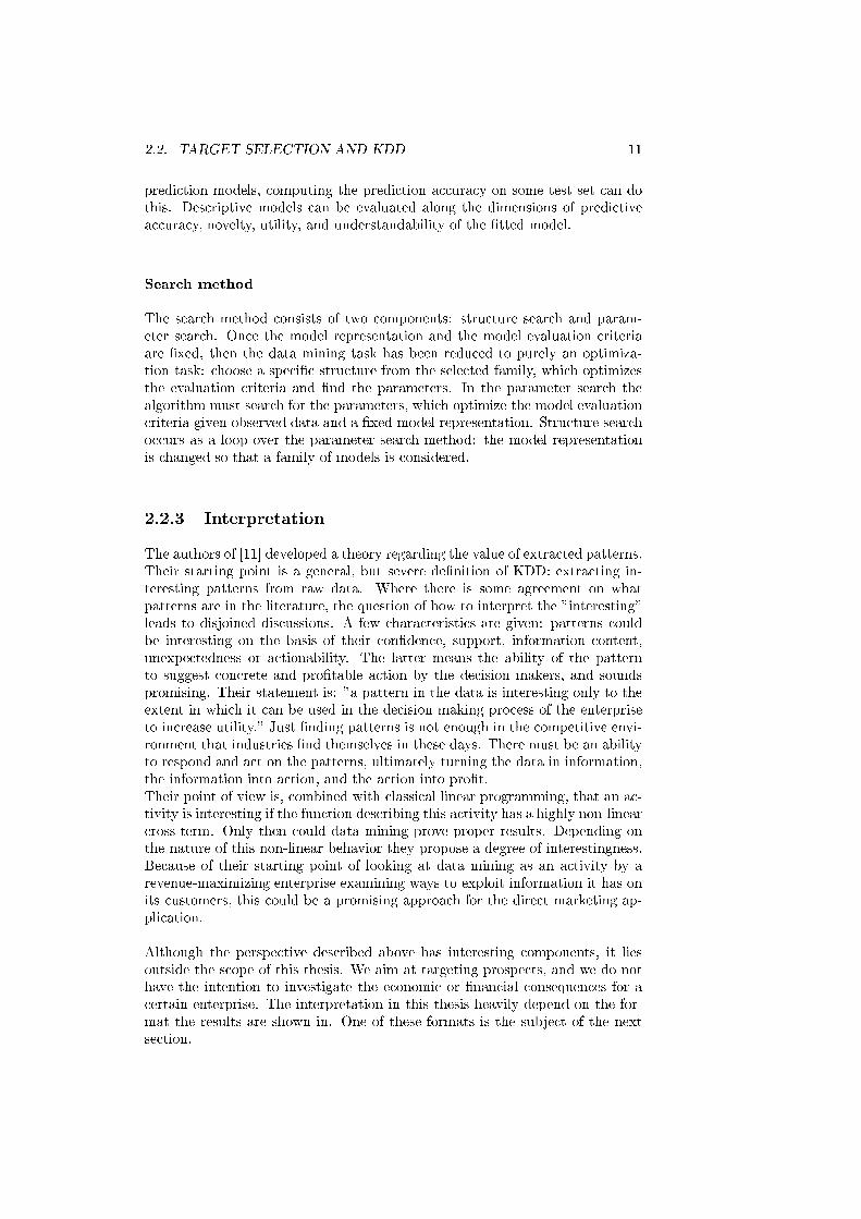
In this thesis, many results will be given in the form of a gain chart. The
ultimate goal is to get the gain chart to leave and continue as vertical as pos-
sible, which means that more valuable prospects are identi�ed. In other words,
the goal is to try to increase the skewness of the gain chart. A example shows
how gain charts are interpreted. If we consider the example gain chart of �gure
2.1, the dashed line would represent an ideal gain chart: by mailing less then
one-tenth of the total customer group all the respondents are found. The other
extreme is when no target selection is used, but just a random mailing. The
resulting gain chart for this case is the dotted one. No gains are obtained by a
random mailing. The typical gain chart (solid curve) lies somewhere between
the two extremes. In this particular case, by mailing 20 % of the total group
around 50 % of the respondents are "caught". Another observation is that there
are no respondents in the last 17 % of the total group.
2.3. GAIN CHARTS 13
0 20 40 60 80 1000
20
40
60
80
100
customers mailed [%]
resp
onde
nts
targ
eted
[%]
GAIN CHART example
Figure 2.1: Gain chart explanation

14 CHAPTER 2. TARGET SELECTION IN DIRECT MARKETING

Chapter 3
Mining algorithms
There are many algorithms available for the purpose of Target Selection. Al-
though not one universal algorithm exists, some do better than others. The core
of the decision process is a response model whose purpose is to assess the pur-
chase propensity of each customer in the list prior to the mailing, as a function
of the customers attributes and purchase history. A variety of approaches have
been developed in the database marketing industry to model response, tradi-
tional human-driven segmentation methods involving RFM (recency, frequency
and monetary) variables [19], tree-structured "automatic" segmentation models
such as Automatic Interaction Detection (AID) [14] [17] [18], Chi Square AID
(Chaid) [8], Classi�cation and Regression Trees (Cart) [13] and C4.5 [24], linear
statistical models such as linear [30], multiple regression [23] and discriminant
analysis [25], non-linear discrete choice logit [9] [20] and probit [22] models. Lin-
ear regression is one of the algorithms which are subject of study. Although the
relationship between the dependent and independent variables is not expected
to be linear, this algorithm can prove reasonable results and has been chosen
as a benchmark. Chaid and logit are also used in this project. These two are
the most commonly applied algorithms in response modeling, and have proven
good results [16].
Recent developments in arti�cial intelligence (AI) have triggered the use of AI-
based methods to model response. Of these methods, arti�cial neural networks
[21] and fuzzy modeling [7] are two examples which will be investigated, because
we hope that these algorithms can deal with the assumed high complexity.
In this chapter, the theoretical background of the �ve models will be covered
together with some additional implementation issues and commends on how to
set up the optimal con�guration. Starting with linear regression in section 3.1,
the logit model follows in section 3.2, Chaid in section 3.3, the Neural Networks
in section 3.4, and �nally the Fuzzy modeling in section 3.5. Each section ends
with a "conclusion" in which we address the individual strengths and weak-
nesses of the technique and then there are some direct comparison of techniques
in terms of:
� Clarity and explicability. The transparency of the model is discussed here:
can the decisions made by the model be explained?
� Implementation and integration
15

16 CHAPTER 3. MINING ALGORITHMS
� Data requirements (including comments on the variable types)
� Accuracy of model
� Construction of model
Finally, in section 3.6 the algorithms are shortly compared and general com-
ments are made about their di�erences based on the individual strengths and
weaknesses sections.
3.1 Linear regression
The �rst method used is linear regression, which belongs to the family of re-
gression models. Regression models view observations on certain events as the
outcome of a random experiment. The outcomes of the experiment are assigned
unique numeric values. The assignment is one-to-one; each outcome gets one
value, and no distinct outcomes receive the same value. This outcome vari-
able, Y , is a random variable because until the experiment is performed, it is
uncertain what value Y will take. Probabilities are associated with outcomes
to quantify this uncertainty. Thus, the probability that Y takes a particularly
value, y, might be denoted Prob(Y = y). So, in target selection if an individual
responds, this is noted as (Y = 1), if not (Y = 0). The regression approach
believes that a set of factors, gathered in a vector x, explains the decision, so
thatProb(Y = 1) = F (�Tx)
Prob(Y = 0) = 1� F (�Tx):(3.1)
The set of parameters � re ect the impact of the changes in x on the probability.
The response (discrete values 0 and 1) in linear regression is described in the
linear regression equation:
y = �Tx+ u (3.2)
In this equation, u represents the error term, of which the expected value is
zero. Put in other words, the error term can take values other than zero, but
on average it equals zero. Assuming that we have the availability of y and x in
a data set, we can calculate an estimate b for �. Now we can give a prediction
for y, or likelihood of response:
by = bTx (3.3)
The error made in this prediction, is called a residual and is de�ned by:
e = y � by (3.4)
The prediction or estimation is usually done by ordinary least square (OLS)
estimation. The basic idea of OLS is to choose those bi's to minimize the sum
of squared residuals:nX1
e2
i; (3.5)
in which n represents the number of customers. It can be proven that minimiz-
ing equation 3.5 results in the following estimate for �:
b = (xTx)�1xTy (3.6)

3.1. LINEAR REGRESSION 17
When a test set comes up with an estimate for �, equation 3.3 can be used to
predict a likelihood of response for the prospects whose characteristics x are
known.
Now that the mathematical framework is described, the assumptions structuring
linear regression are looked into. These Gauss-Markov assumptions guarantee
that the estimates will have good properties [30].
3.1.1 Linear regression assumptions
1. E(u) = 0, the expected value of the errors is zero
2. The independent variables are non-random (and have �nite variances)
3. The independent variables are linearly independent. Failure of this as-
sumption is called multicollinearity (singularity).
4. E(u2 = �2), the disturbances ui are homoscedastic: the variance of
disturbance is the same for each observation.
5. E(uiuj) = 0 8 i 6= j, disturbances associated with di�erent observations
are uncorrelated.
If the assumptions 1 to 3 are satis�ed, then the OLS estimator b will be unbi-
ased: E(b) = �. Unbiasedness means that if we draw many di�erent examples,
the average value of the OLS estimator based on each sample will be the true
parameter value �. If all 5 assumptions hold, the variance of the OLS esti-
mator equals Var(b) = �2(xTx)�1. If the independent variables are highly
correlated, the matrix xTx will become nearly singular and the elements of
(xTx)�1 will be large, indicating that the estimates of � may be imprecise.
The assumptions mentioned above have some important e�ects on the con-
�guration in which linear regression will perform best.
3.1.2 Feature selection and correlation
Because the following feature selection procedure is also based on linear rela-
tionships, it is mentioned here.
The overall aim is to keep the number of attributes as low as possible in order
to reduce the model complexity. A real-life data set can contains hundreds of
variables, which have to be reduced to a number around or lower than ten. This
value is arbitrarily, but the less features the better.
We recall the correlation coeÆcient:
�(xk; y) =
1
n
Pi(xik � �xk)(yi � �y)
�xk�y
: (3.7)
If we use these correlation coeÆcients of the variables, the following selection
reduces the number of features (the model complexity). Only select those at-
tributes that have an high absolute correlation with the the dependent attribute
compared to the other attributes. If we use a threshold of at least two times

18 CHAPTER 3. MINING ALGORITHMS
larger, features xk are included if they satisfy the condition given in equation
3.8.
j�(xk; y)j >2
K
Xk
j�(xk; y)j: (3.8)
3.1.3 Strengths and weaknesses
Probably the most important constraint of linear regression is that is not able
to directly1 account for non-linear relations. On the other hand, the main
advantage is the ease of constructing and understanding the model. Another
advantage is that the dependent variable can take any value. All dependent
attributes are treated as continuous. Although F-tests can be applied, linear
regression does not have straight-forward feature selection capabilities.
3.2 Logit
The second method, which will be used in modeling the individuals, is known
as logistic regression or logit analysis, logit in short. Since that the dependent
variable is binary: either there is a response or not, this form of regression is
referred to as binominal logistic regression.
The following mathematical background can be found in [6].
In the logit model the right-hand side of the regression equation is
F (�Tx) =exp(�Tx)
1 + exp(�Tx): (3.9)
The estimation of a logit model is usually based on the method of maximum
likelihood. Each observation is treated as a single draw from a Bernoulli distri-
bution (binominal with one draw). We call the estimate for � b. The model
with success probability F (bTx) and independent observations leads to the
joint probability or likelihood function:
L = Prob(Y1 = y1; Y2 = y2; :::; Yn = yn) =Yyi=0
�1�F (bTx)
� Yyi=1
�F (bTx)
�(3.10)
Taking the logs, we obtain the log-likelihood, G:
G = lnL =Xi
�yi lnF (b
Tx) + (1� yi) ln
�1� F (bTx)
��(3.11)
The �rst-order conditions for maximization require setting the gradient to zero:
g =@G
@b=Xi
(yi � F (bTxi)xi = 0 (3.12)
The second derivatives for the logit model are based on:
H =@2G
@b@bT= �
Xi
F (bTxi)(1� F (bTxi))xixTi
(3.13)
1Transformations such as a log transformation can be done if the attributes have logarith-
mic distributions (non-linear).

3.2. LOGIT 19
The Hessian is always negative de�nite, so the log-likelihood is globally con-
cave. It will usually converge to the maximum of the log-likelihood in just a
few iterations unless the data are especially badly conditioned. The asymptotic
covariance matrix for the maximum likelihood estimator can be estimated by
using the inverse of the Hessian evaluated at the maximum likelihood estimates.
The initial coeÆcients are compute by ordinary least squares estimation: then
the log-likelihood is maximized with respect to the beta-vector. This can be
done by applying Newton's method, which implies the following iteration (num-
ber of iterations is denoted by t):
bt+1 = bt �H�1gt (3.14)
The estimate for the beta vector is updated until a certain convergence criterion
is met or a maximum number of iterations has been exceeded.
If the dependent variable has more than two classes, one could apply a multi-
nominal logit. More about this subject and other binary choice models, can be
found in [9] and [6].
3.2.1 Implementation and veri�cation
The logit algorithm is implemented according to the procedure of 3.2. In this
section a simple example is used to show that the algorithm works correctly.
The Matlab implementation of the logit algorithm used can be found in ap-
pendix ??, and is called logit.m. A simple example is used to test the algorithm.
The example comes from [6], and is listed in table 3.1. This particular data set
Table 3.1: Spector and Mazzeo data
gpa tuce psi grade gpa tuce psi grade
2.66 20 0 0 3.28 24 0 0
4.00 21 0 1 2.76 17 0 0
3.03 25 0 0 2.63 20 0 0
3.57 23 0 0 3.53 26 0 0
2.75 25 0 0 3.12 23 1 0
2.06 22 1 0 2.89 14 1 0
3.54 24 1 1 3.39 17 1 1
3.65 21 1 1 3.10 21 1 0
2.89 22 0 0 2.92 12 0 0
2.86 17 0 0 2.87 21 0 0
3.92 29 0 1 3.32 23 0 0
3.26 25 0 1 2.74 19 0 0
2.83 19 0 0 3.16 25 1 1
3.62 28 1 1 3.51 26 1 0
2.83 27 1 1 2.67 24 1 0
4.00 23 1 1 2.39 19 1 1
was used to analyze the e�ectiveness of a new teaching method. The dependent
20 CHAPTER 3. MINING ALGORITHMS
variable is "grade", an indicator whether students' grades on examination im-
proved after exposure to "psi" (exposed or not), a new teaching method. The
other variables are "gpa", the grade point average; and "tuce", the score on a
pre-test which indicates entering knowledge of the material. The implemented
logit algorithm showed similar results: the coeÆcients and t-ratios matched per-
fectly even in the third decimal. In table 3.2 the coeÆcients obtained by logit
and the known coeÆcients are listed for this Spector and Mazzeo data set.
Table 3.2: CoeÆcients and t-ratios compared
logit Greene logit Greene
Coe� Coe� t-ratio t-ratio
beta -13.021347 -13.021 -2.640538 -2.640
gpa 2.826113 2.826 2.237723 2.238
tuce 0.095158 0.095 0.672235 0.672
psi 2.378688 2.379 2.234425 2.234
The only two parameters which can (default values are inhibited) be adjusted
by the user are the maximum number of iterations or the convergence criterion.
Testing the algorithm resulted in the observation that 6 iterations are enough
for good results: even if the default convergence criterion (1 � 10�6) is not
met, results do not change signi�cantly when more iterations are made.
Although the algorithm itself proves good results stand-alone, in this stage it can
not be used as a target selection algorithm. Some adjustments and additional
operations have to be applied before logit works as an proper target selection
method. These issues will be covered in the remainder of this section, resulting
in a "optimized" target selection algorithm.
3.2.2 Scaling
Scaling seems to be an plausible technique for logit, because in the implementa-
tion the t-test is used to look whether a calculated coeÆcient signi�cantly di�ers
from zero. If no scaling is applied, features with a large value scale will tend
to be more signi�cant than attributes with a modest scale. Therefore, all the
variables are scaled to zero mean and variance one, a common transformation.
3.2.3 Feature selection
The last remark on the logit con�guration, probably the most important issue,
is how the feature selection can be done? Feature selection is the process of
eliminating features until only signi�cant features, the best predictors, are left.
This can be done in the following way:
First, 100 random selections are made from the data set. On each of this
selection the logit algorithm is performed. Then, sub-selections are chosen based
on the signi�cant features denoted by the previous run. In other words, the
least important attributes are eliminated from the data set, based on the t-test
of signi�cance. This is repeated until the resulting data sets can no more be
reduced, the features in the data set are all signi�cant. Every selection assigns
his own set of signi�cant predictors. The signi�cant features of each selection

3.3. CHAID 21
are tabled, and for each feature is calculated by how many of the 100 selections
it was found to be signi�cant.
T-test
In order to determine which features have more impact on the dependent then
other, a t-test can be used. Basically, the t-test on the logit coeÆcients tests
whether a coeÆcient di�ers from zero, and expresses this with a degree of sig-
ni�cance, the so-called t-statistic. At the 95 % signi�cance level the t-ratio for
the estimate of a coeÆcient is 1.96. The mathematical background of the t-test
can be found in [6].
3.2.4 Strengths and weaknesses
Logit is known as a hard benchmark to beat: usually logit �nds itself among
the best performing algorithms in target selection environments [16]. However,
logit does not automatically account for interaction e�ects [29]. Logit does not
assume a linear relationship between the dependent and the features, but it
does assume a linear relationship between the "logit" (see equation 3.9) of the
features and the dependent. It may handle nonlinear e�ects even when expo-
nential and explicit interaction and power terms can be added as extra features,
but logit does not account for these e�ects automatically.
Another problem that can occur is known as multicollinearity. This means that
the features are linear functions of each other. To the extent one variable is a
linear function of other variables, the reliability of the estimate of the coeÆcient
for this variable decreases [29].
Logit treats all feature values as continuous, just as linear regression. One
requirement regarding the data is due to the use of maximum likelihood estima-
tion: this procedure implies that the reliability of estimates decline when there
are few cases for each observed combination of the variables. So, large samples
increase the reliability.
3.3 Chaid
Chaid belongs to the set of decision trees. It is used for classi�cation and pre-
diction purposes. It has been successfully used to identify target groups of
customers for direct mail for many years.
A decision tree represents a series of questions or rules, based on independent
variables, shown as a path through the tree. Oddly, decision trees are shown
going down from the root tree node towards the leaf tree nodes. A decision tree
can be built using an algorithm that splits records into groups where the prob-
ability of the outcome di�ers for each group based on values of the independent
variables. Chaid was �rst introduced in [8] as an extension from a technique
called Automatic Interaction Detection (AID). Chaid uses the chi squared test
to determine whether to branch further and if so which independent variables to
use. Hence it's name Chi Squared Automatic Interaction Detection (CHAID).
It was developed to identify interactions for inclusion into regression models.
Chaid easily copes with interactions, which can cause other modeling techniques

22 CHAPTER 3. MINING ALGORITHMS
diÆculty. Interactions are combinations of independent variables that a�ect the
outcome. For instance, pro�tability may be at the same level for low transac-
tions in combination with high balance credit customers as for high transaction
with low balance credit customers; in this case of modeling pro�tability, these
two independent variables (transactions and balance) should not be considered
in isolation.
The Chaid algorithm splits records into groups with the same probability of
the outcome, based on values of independent variables. The algorithm starts at
a root tree node, dividing into child tree nodes until leaf tree nodes terminate
branching. Branching may be binary, ternary or more. The splits are deter-
mined using the chi squared test. This test is undertaken on a cross-tabulation
between outcome and each of the independent variables. A cross-tabulation is
a kind of frequency table: for each category of the predictor and each value
of the dependent, the individuals with the same category value in combination
with the same dependent value are counted and their sum is put into the cross-
tabulation. The result of the test is a "p-value". The p-value is the probability
that the relationship is spurious, in statistical jargon this is the probability that
the Null Hypothesis is correct. The p-values for each cross-tabulation of all the
independent variables are then ranked, and if the best (the smallest value) is be-
low a speci�c threshold then that independent variable is chosen to split the root
tree node. This testing and splitting is continued for each tree node, building a
tree. As the branches get longer there are fewer independent variables available
because the rest has already been used to further up that branch. The splitting
stops when the best p-value is not below the speci�c threshold. The leaf tree
nodes of the tree are tree nodes that did not have any splits with p-values be-
low the speci�c threshold or all independent variables are used. This outlines a
purely automated approach to building a tree. The best trees are built when a
model builder checks each split and makes rational decisions (using background
domain knowledge) as to the appropriateness of splitting on a particular vari-
able at a speci�c point. The model builder can spot splits using independent
variables that raises questions as to quality, hence avoiding problems of building
an invalid tree, or model, on poor input data. A model builder may also decide
to stop splitting at a higher level than the automated approach would stop, in
order to produce a simpler model.
The step-wise procedure for Chaid as stated in [8] is as follows:
1. For each predictor in turn, cross-tabulate the categories of the predictor
with the categories of the dependent variable and do steps 2 and 3.
2. Find the pairs of categories of the predictor (only considering allowable
pairs as determined by the type of predictor) whose 2 by 2 sub-table
is least signi�cantly di�erent. If this signi�cance does not reach a critical
value, merge the two categories, consider this merger as a single compound
category, and repeat this step.
3. For each compound category consisting of three or more of the original
categories, �nd the most signi�cant binary split (constraint by the type of
the predictor) into which the merger may be resolved. If this signi�cance

3.3. CHAID 23
is beyond a critical value, implement the split and return to step 2. 2
4. Calculate the signi�cance of each optimally merged predictor, and isolate
the most signi�cant one. If this signi�cance is greater than a criterion
value, subdivide the data according to the (merged) categories of the cho-
sen predictor.
5. For each partition of the data that has not yet been analyzed, return to
step 1. This step may be modi�ed by excluding from further analysis
partitions with a small number of observations.
3.3.1 The chi square test
The �rst step in computing the chi square test of independence is to compute the
expected frequency for each cell in the cross-tabulation under the assumption
that the null hypothesis is true. To put it in other words: calculate the expected
cell frequencies assuming that the compared features are independent. The
general formula for expected cell frequencies is:
Eij =TiTj
N(3.15)
where Eij is the expected frequency for the cell in the i-th row and j-th column,
Ti is the total number of subjects in the i-th row, Tj is the total number of
subjects in the j-th column, and N is the total number of subjects in the whole
table. The formula for chi square test of independence is:
�2 =
Xij
(Eij � aij)2
Eij
(3.16)
where aij is the value of the cross-tabulation in the i-th row and j-th column .
The degrees of freedom (df) are equal to (R� 1)(C � 1), where R is the
number of rows and C the number of columns. Now, a chi square table can be
used to determine the probability for the calculated �2 and df .
3.3.2 Signi�cance of the predictors
Step 4 of the Chaid algorithm requires a test of signi�cance of the reduced
contingency table. If there has been no reduction of the original contingency
table, a chi square test can be used.This test is conditional on the number of
categories of the predictor, otherwise it must be viewed as conservative.
If categories have been merged in a predictor, a Bonferroni multiplier can be
used according to [8]. This is needed to account for the number of ways a c
category predictor of a given type can be reduced to r groups (1 � r � c).
The formulae for calculating these multipliers for the three types of predictor
allowed by Chaid are:
2This third step does not specify how to �nd the required binary split. Using direct search,
�nding an optimal binary split for nominal variables requires time that is exponential in the
number of categories.

24 CHAPTER 3. MINING ALGORITHMS
1. Monotonic predictors. As in AID, a monotonic predictor is one whose
categories lie on an ordinal scale. This implies that only contiguous cate-
gories may be grouped together. In this case the Bonferroni multiplier is
equal to the binomial coeÆcient [8]:
Bmon =
�c� 1
r � 1
�(3.17)
2. Free predictors. Again as in the conventional AID, a free predictor is one
whose categories are purely nominal. This implies that any grouping of
categories is permissible. In [8], the multiplier is derived as:
Bfree =
r�1Xi=0
(�1)i(r � i)c
i!(r � i)!(3.18)
3. Floating predictors. In some practical cases, the categories of a predic-
tor lie on an ordinal scale with the exception of a single category that
either does not belong with the rest, or whose position on the ordinal
scale is unknown (like in�nity or not-a-number). This is de�ned as the
oating category, and the predictor is called a oating predictor. Again,
the Bonferroni multiplier is derived in [8]:
Bfloat =r � 1 + r(c� r)
c� 1Bmon (3.19)
3.3.3 Implementation
Chaid is not implemented in Matlab. SPSS Chaid has been used instead. The
reason is the lack of suÆcient information on some critical decision points in
the implementation. More information on SPSS Chaid can be found in [32].
3.3.4 Strengths and weaknesses
The form of a Chaid tree is intuitive, it can be expressed as a set of explicit
rules in English. This means that the business user can con�rm the rationale
of the model and if necessary, modify the tree or direct it's architecture from
their own experience or their background domain knowledge. Input data quality
problems can be spotted, hence problems of building an invalid model on poor
input data can be avoided. Also the most important predictors (or independent
variables) can easily be identi�ed and understood.
A Chaid model can be used in conjunction with more complex models. For
instance, a Chaid model could identify who may be at risk of leaving and then
a more complex pro�t model could be used to determine whether the customer
is worth keeping.
Chaid models can handle categorical (like marital status) and banded continu-
ous independent variables (like income). Continuous independent variables, like
income, must be banded into categorical-like classes prior to use in Chaid. In
particular if the independent variables are categorical with high cardinality (im-
plicit "containing" relationships) Chaid should perform even better. A Chaid
model can automatically prevents over-�tting and handle missing data. Chaid

3.4. NEURAL NETWORKS 25
does not require much computational power.
Chaid needs rather large volumes of data to ensure that the number of observa-
tions in the leaf tree nodes large enough to be signi�cant. Continuous variables
must be banded.
3.4 Neural Networks
Neural Networks (NNs) are biologically inspired models which try to mimic the
performance of the network of neurons, or nerve cells, in the human brain. Ex-
pressed mathematically, a NN is made up of a collection of processing units
(neurons, nodes), connected by means of branches, each characterized by a
weight representing the strength of the connection between the neurons. On
the �rst try, since the NN is still untrained, the input neuron will send a current
of initial strength to the output neurons, as determined by the initial conditions.
But as more and more cases are present, the NN will eventually learn to weight
each signal appropriately. Then, given a set of new observations, these weights
can be used to predict the resulting output.
Neural Networks are often mentioned in many theoretical and practical jour-
nals as a promising and e�ective alternative to conventional response modeling
in database marketing for targeting audiences through mail promotions. NNs
employ the results of a previous mailing campaign, for which it is known who
responded with an order, and who declined, to train a network and come up
with a set of "weights", each representing the strength of connection between
any two linked nodes, or neurons, in the network. These weights are then used
to score the customers in the data set and rank them according to their likeli-
hood of purchase; usually, the higher the NN score, the higher the propensity
to purchase.
The neurons are usually grouped in several layers. One input layer, one or more
"hidden" layers and an output layer. One example of a Neural Network used
in this thesis is the so-called one-layer supervised Feedforward-Backpropagation
Neural Network.
3.4.1 The feedforward-backpropagation NN
Supervised means that the NN gets both the input and known output values.
Feedforward, because the only direction for information ow is from the input
layer to the output layer. In this way, from the inputs the outputs of the �rst
layer are calculated. These form the input of the second hidden layer, and this
goes on until the output layer has been reached. The input layer neurons do
not perform any computations, but merely distribute the inputs xi (i = 1 : p)
to the weights whij of the hidden layer (j represents the number of neurons
in the layer). The weighted inputs are add up for each neuron (resulting in
a value zj) and passed through a non-linear function �, which is called the
activation function. The value of this function vj = �(zj) is the output of the
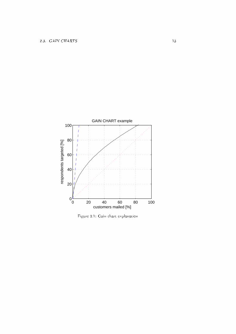
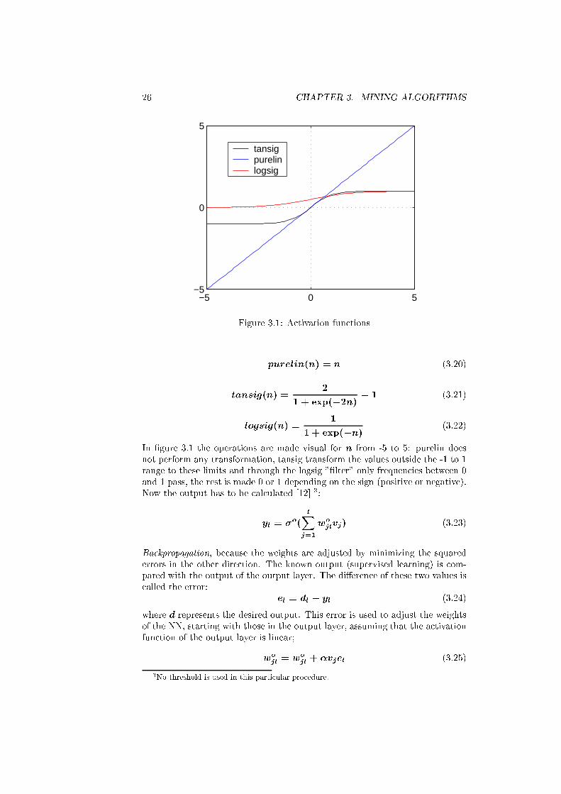
neuron. There exist several activation functions. The three activation functions
most commonly used are: Purelin, Tansig and Logsig. The transformations are
de�ned as follows:
26 CHAPTER 3. MINING ALGORITHMS
−5 0 5−5
0
5
tansig purelinlogsig
Figure 3.1: Activation functions
purelin(n) = n (3.20)
tansig(n) =2
1 + exp(�2n)� 1 (3.21)
logsig(n) =1
1 + exp(�n)(3.22)
In �gure 3.1 the operations are made visual for n from -5 to 5: purelin does
not perform any transformation, tansig transform the values outside the -1 to 1
range to these limits and through the logsig "�lter" only frequencies between 0
and 1 pass, the rest is made 0 or 1 depending on the sign (positive or negative).
Now the output has to be calculated [12] 3:
yl = �o(
lXj=1
wojlvj) (3.23)
Backpropagation, because the weights are adjusted by minimizing the squared
errors in the other direction. The known output (supervised learning) is com-
pared with the output of the output layer. The di�erence of these two values is
called the error:
el = dl � yl (3.24)
where d represents the desired output. This error is used to adjust the weights
of the NN, starting with those in the output layer, assuming that the activation
function of the output layer is linear;
wojl= w
ojl+ �vjel (3.25)
3No threshold is used in this particular procedure.

3.4. NEURAL NETWORKS 27
Then we adjust the hidden layer weights, mathematically expressed as:
whij = w
hij + �xi�
Tj (zj)
Xl
elwojl (3.26)
Before the training can start, the weights have to be randomly initialized. The
updating of the weights is repeated until the error has reached a criterion value.
One run is called an epoch.
3.4.2 Implementation
The neural network toolbox version 3.0.1 (R11) is used. The function "new�"
builds a feed-forward back-propagation network. As training function is chosen
for "trainlm": the Levenberg-Marquardt back-propagation training.
3.4.3 Strengths and weaknesses
NNs can be applied to both directed (supervised) and undirected (unsupervised)
data mining. NNs can handle both categorical and continuous independent vari-
ables without banding.
NNs can produce a model even in situations that are very complex because an
NN produces non-linear models.
The independent variables must be converted into the range from 0 to 1, this
is done using "transformations" which can be inaccurate when the independent
variables are skewed with a few outliers.
The output from an NN is usually continuous which may be diÆcult to trans-
form to a discrete categorical outcome.
Several parameters must be set up, for instance the number of hidden layers
and the number of nodes per hidden layer. These parameters a�ect the model
built. The results of small di�erences in these parameters can be the di�erence
between a very predictive model and a poor model. So, experience in building
NNs is almost a demand for a fair con�guration.
The results of an NN cannot be explained, it is a "black-box", a set of weights
with no inherent meaning. Recently, some explanation of an NN may be ob-
tained by using additional techniques to visualise the networks and to produce
rules from prototypes (using sensitivity analysis). Explicability is a legal re-
quirement for credit product application models in the US, this means that
NNs cannot be used to build credit risk models. The lack of clarity means that
unfair prejudice cannot be ruled out from the credit decision.
NNs can produce models that are sub-optimal.
To build an NN model requires an experienced statistician or expert NN user
to ensure that the model is not over-�tted.
This method can be very time-consuming because of the number of re-presentations
of the data that is required during training. Also if there is a large number of
predictive variables, then the time taken to �nd a solution are further length-
ened. The skill and e�ort required to build an NN plus the time involved means
that this technique is costly.

28 CHAPTER 3. MINING ALGORITHMS
3.5 Fuzzy modeling
The fuzzy modeling algorithm used in this thesis is proposed and fully described
in [7]. In this section a short review is given.
Although the model presented has an procedure to deal with missing values
(see section 2.2), pre-processing tasks are not further mentioned in this section.
The model follows the two-fold analysis of direct marketing campaigns: �rst
feature selection must determine the variables that are relevant for the speci�c
target selection problem. Second, rules 4 for selecting the customers should be
determined, given the relevant features.
3.5.1 Feature selection
In this fuzzy model, feature selection is done using gain charts from individual
models made for each variable. This means that each variable is modeled using
fuzzy c-means clustering, which allows cluster merging and variable sized cluster
prototypes, and gain analysis, leading to additive improvement of the gain charts
per feature and to the total model as models of individual features are added to
the total model in a decision tree like manner. First the clients (k = 1 : N) are
ranked per feature (j = 1 : n). By assigning a fuzzy Respondent Density (RD)
for each cluster Mj of each variable j, which represents the ratio of the total
membership of the positive respondents in the cluster to the total membership
of all clients N in the cluster.
RDij =
PN
k=1�ij(xkj)ykPN
k=1�ij(xkj)
; 1 � i �Mj; j = 1; 2; :::; n (3.27)
In equation 3.27 �ij(xkj) represents the membership of the k'th client in the
i'th cluster of feature j. These RD values are then used to compute a score
(SC) for each client for each feature.
SCjk =
MjXi=1
�ij(xkj)RDij ; 1 � k � N (3.28)
The score SC for each client for each feature is made up of a weighted sum over
all clusters of the product of the membership value for each cluster, the value of
the client for the particular feature and the RD value for the cluster. By doing
so, the higher the SC score, the more plausible that the particular client is a
respondent, according to the feature examined. Next, gain charts are calculated
for each feature. Each gain chart is assigned a score SX which re ects its
targeting eÆciency. Feature selection can now be done in an iterative manner,
the feature with the highest SX score, e.g. the most favorable gain chart, is the
most important feature according to this methodology. The cluster centers and
the corresponding RD values for the selected feature are recorded as part of the
�nal model. Now the clients whose SC scores for the most important feature
4Rules are preferred, because domain experts can verify them with their experience. Some
algorithms (like NNs) do not come up with explicit rules but do result in a selection model
that can assign an index of prosperity to a individual (see section 3.6 for more information on
this subject).

3.6. SUMMARY OF TARGET SELECTION ALGORITHMS 29
are in fact the highest SC scores compared to all SC score for the other features,
are removed from the data set.
In this way, the clients that are best described by this feature are identi�ed.
This process continues until a maximum depth is met, in other words a (user
speci�ed) maximum number of important features is reached. Other stopping
criteria are possible: for example, the process stops when no more respondents
are left in the data set (all respondents are described by the selected features).
3.5.2 Target selection
Now that the subset with the most attractive features is found, the individual
models of each feature are combined in a �nal model. The ranking and selection
of the clients is done by averaging the results from each feature. The target
selection score for a client is the sum of the SC scores of the feature subset
divided by the number of features in this set.
3.5.3 Strengths and weaknesses
The fuzzy modeling technique makes it possible to capture some of the struc-
tures in the data for which one normally would have to consider the interactions
between the features [7].
The fuzzy modeling approach provides an advantage to many other AI tech-
niques, since the model can be represented in a rule-based form that analyst
can verify against their own knowledge and experience.
Because of the rather complex structure of the fuzzy modeling technique, many
calculations have to be made. This is the reason why the algorithm is quite
time consuming compared to a method like Chaid.
3.6 Summary of target selection algorithms
In this section we shortly review all �ve target selection algorithms and discuss
their di�erences and suitability.
The �rst remark addresses the availability of suÆcient data. Although all tar-
get selection algorithms need representative train samples, Chaid requires more
samples than the other four algorithms. If there are not enough discriminating
attributes, Chaid can better be used for feature selection and another method to
score the prospects. This is because in the case of a few leaf nodes, Chaid assigns
just a few di�erent scores for all prospects. On the other hand, a Chaid tree is
relatively easy to build, and available in several commercial software packages.
It is, however, diÆcult to implement Chaid yourself, not because of the diÆcult
structure but because of the lack of relevant background information on several
speci�c choices.
Neural networks are quite laborious: the number of neurons in the hidden layer
has to be determined by trail and error. Furthermore, the time to train a neural
network can be quite long, especially in case of a large number of attributes and
the network is a blackbox; no linguistic rules can be deducted like the Chaid
and fuzzy modeling algorithm do have this capability. The fuzzy modeling tech-
nique has another advantage: it handles the feature selection and client scoring

30 CHAPTER 3. MINING ALGORITHMS
in the same computational procedure. One disadvantage is that the training
requires a lot of time compared to Chaid and the regression techniques. Logit
and linear regression are fast procedures, but because the procedures involve
matrix inversion, not all data sets can be presented, especially if they are bad
conditioned. So, these algorithms are in particular suitable for the task of client
scoring where another algorithm should determine the relevant features.
Recapitulating, based on the di�erences between the models feature selection
can be best done by Chaid and the fuzzy modeling algorithm. The feature
selection procedure described in section 3.1.2 is very easy and based on linear
relationships. For the purpose of client scoring, linear and logistic regression,
neural networks and the fuzzy modeling algorithm are suited best. The latter
is best used without external feature selection because this can demolish the
speci�c structures which the fuzzy modeling technique tries to �nd.
Chapter 4
Methodology
In this chapter the previous two chapters are used in order to derive the method-
ology to really conduct some "intelligent" target selection. This chapter can be
roughly divided in three main parts. The �rst part is the introduction of the
data set and its treatment as application domain. In this way, the abstract
theory of the KDD cycle is employed in a real business problem. By doing so,
we believe that the di�erent steps are explained in a clearer way to the reader.
The second part is an explanation of di�erent numerical performance measures
which will be used to compare the di�erent con�gurations. The measures even-
tually used, are derivatives of the gain chart analysis (section 2.3). The last and
most important part is the practical �lling of the KDD cycle of chapter 2: the
methodology to come up with the di�erent con�gurations for intelligent target
selection in direct marketing.
4.1 Data set and direct marketing
The data set used in this thesis work is a real-life data set used in a contest and
very representative for all issues concerned in deploying target selection in direct
marketing. The original assignment and description of this data set follows �rst.
The rest of this section tries to give the answers to the �ve questions, typical
for direct marketing campaigns, as mentioned in chapter 2.
4.1.1 Original TIC assignment
"Direct mailings to a company's potential customers, many of them see this as
"junk mail", can be a very e�ective way for them to market a product or a
service. However, as we all know, much of this junk mail is really of no interest
to the people that receive it. Most of it ends up thrown away, not only wasting
the money that the company spent on it, but also �lling up land�ll waste sites
or needing to be recycled. If the company had a better understanding of who
their potential customers were, they would know more accurately who to send it
to, so some of this waste and expense could be reduced. So here is our challenge:
Can you predict who would be interested in buying a caravan insurance pol-
icy and give an explanation why?
31
32 CHAPTER 4. METHODOLOGY
The competition consists of two tasks:
1. Predict which customers are potentially interested in a caravan insurance
policy.
2. Describe the actual or potential customers; and possibly explain why these
customers buy a caravan policy.
Participants need to provide a solution for both tasks. We want you to pre-
dict whether a customer is interested in a caravan insurance policy from other
data about the customer. Information about customers consists of 86 variables
and includes product usage data and socio-demographic data derived from zip
area codes. The data was supplied by the Dutch data mining company and is
based on a real world business problem. The training set contains over 5000
descriptions of customers, including the information of whether or not they
have a caravan insurance policy. A score set contains 4000 customers which you
will classify. A portion of your performance will be judged on your accuracy
of classi�cation of this set. For the prediction task, the underlying problem
is to the �nd the subset of customers with a probability of having a caravan
insurance policy above some boundary probability. The known policyholders
can then be removed and the rest receives a mailing. The boundary depends
on the costs and bene�ts such as of the costs of mailing and bene�t of selling
insurance policies. To approximate this problem, we want you to �nd the set
of 800 customers in the score set that contains the most caravan policy own-
ers. For each solution submitted, the number of actual policyholders will be
counted and this gives the score of a solution. Only the indexes of the selected
records need to be provided, assuming that the �rst record has index number
1 (e.g. 1,7,24,...,3980,4000). The purpose of the description task is to give a
clear insight to why customers have a caravan insurance policy and how these
customers are di�erent from other customers. Descriptions can be based on
regression equations, decision trees, neural network weights, linguistic descrip-
tions, evolutionary programs, graphical representations or any other form. The
descriptions and accompanying interpretation must be comprehensible, useful
and actionable for a marketing professional with no prior knowledge of com-
putational learning technology. Since the value of a description is inherently
subjective, submitted descriptions will be evaluated by experts in insurance
marketing and data mining."
The distinction between the train (tic data set) and �nal validation (score set)
set is very important to keep in mind.
4.1.2 The direct marketing questions
Although the answers to the questions are somewhat straight-forward, they are
instructive and provide a complete overview of the method presented in this
thesis. The �ve questions to be considered for a successful direct marketing
campaign are (see section 2.1):
1. Who am I trying to reach?
Individuals interested in a caravan insurance.

4.2. PERFORMANCE MEASURES 33
2. What do I want them to do?
It is obvious that the prospects should buy a caravan insurance. To lower
the threshold, the intended reaction of the prospects must be made as
easy as possible. If telephone numbers are available, one could consider
phoning the prospects a few days after sending the o�er to ask them about
their interests in caravan insurance policies and their opinion on the o�er.
3. Why should they do it?
This is not completely clear. Nothing is mentioned about an attractive
o�er in the assignment. One could think of discount packages with, for
instance, car insurances.
4. Where should I reach them?
Because the target market is the consumer market, home addresses are
most likely to be used in this particular campaign.
5. When should I reach them?
One thing to consider here is the time of the season. Spring could work,
because people are planning their summer holidays and might be consid-
ering the purchase of a caravan.
4.2 Performance measures
In this section, the model evaluation criteria are de�ned. In order to make
statements about the performance of di�erent target selection con�gurations,
several means of comparison can be used. First of all, scatter matrices can
provide insight in the performance. A scatter matrix for response modeling is
a 2 by 2 matrix in which the rows represent the predicted response y and the
columns the actual response y. In table 4.1 an example of a scatter matrix is
Table 4.1: Example scatter matrix
SCATTER y = 0 y = 1 total
y = 0 654 23 677
y = 1 286 37 323
total 940 60 1000
given. From this table can be seen that 37 out of 60 respondent are successfully
classi�ed, which is equal to 61.6 %. This percentage is denoted as P1. Equally,
the value for P0 in this example is 69.6 %. Although scatter matrices can
provide insight in the percentages of successful classi�cations, there are two
disadvantages of using this measure to compare di�erent con�gurations. It is
not clear which percentage or what combination of P0 and P1 to use. On the one
hand a high value of P1 increases the number of respondents, but this usually
causes P0 to decrease resulting in a higher cost per order. On the other hand,
a large value for P0 increases customer annoyance, which is diÆcult to express
in terms of pro�t loss but still present. Hence, there is a trade-o� between P0and P1 which can not be numerically expressed.
34 CHAPTER 4. METHODOLOGY
4.2.1 Numerical Gain Chart Value
Using gain charts (section 2.3) for comparing di�erent target selection con�gu-
rations is diÆcult when the curves are much alike. Several numerical measures
can be de�ned, a surface measure which would represent the area between the
gain chart curve and the 45 degree reference line (the dotted line in �gure 2.1),
or a measure which represents the percentage respondents targeted at a certain
�xed percentage of the total group mailed. One could think of a certain com-
bination of the two mentioned. Let P20 denote the percentage of respondents
at the 20 percent level of the total group, in the same way: P50 represents the
percentage of respondents when 50 percent of the total groups is mailed. The
measure used is denoted by Numerical Gain Chart Value (NGCV) and is de�ned
by:
NGCV = �(P20 � 0:2) + �(P50 � 0:5) (4.1)
The choice for the weight factors (�; �) is somewhat arbitrarily, the idea behind
it is that the importance of a high skewness of the gain chart is expressed by
the ratio of the two coeÆcients. So, � should be larger than �. The absolute
values are not that important: NGCV is merely a measure to compare several
con�gurations, the value itself does not have a direct meaning: it is made up of
two weighted gain values of response percentages to random selection. In this
line of thought, � can be set to 0.7 and � to 0.3.
4.2.2 CoIL Performance Measure
The performance measure used in the CoIL challenge was the number of re-
spondents in the �rst 20 % of the score set after the prospects are ordered by
a con�guration in terms of the likelihood of response. This number is denoted
by CoIL Performance Measure (CPM). We shall use this performance measure
in this thesis because results can be easily compared to the results of the CoIL
contestants.
4.3 Target Selection by KDD
This section provides the �lling of the Knowledge Discovery in Data cycle as pre-
sented in section 2.2. The intention is to construct the process as autonomously
as possible. This constraint is added because we want to develop some kind
of independent agent who can do the target selection for us and does not need
interference of domain experts who are in general very expensive to consult. We
will now �ll all the gaps in the nine basic steps.
1. Developing an understanding of the application domain.
Domain expertise is gained in section 4.1.2 and the customers' goal of
this KDD process is the purchase of a caravan insurance policy.
2. Selection: create a target data set.
The target data set used in this thesis work, is the training set, men-
tioned in section 4.1. It contains 5822 client records, of 86 attributes each.
The �rst 43 features are zip code characteristics and the rest are features
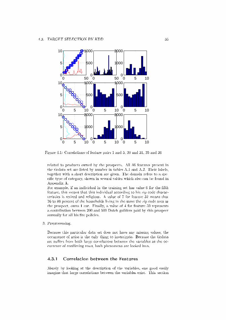
4.3. TARGET SELECTION BY KDD 35
0 500
5
10
0 500
500
1000
0 5 100
1000
2000
0 5 100
5
10
0 5 100
500
1000
0 5 100
500
1000
0 5 100
5
10
0 5 100
1000
2000
0 5 100
1000
2000
Figure 4.1: Correlations of feature pairs 1 and 5, 30 and 31, 35 and 36
related to products owned by the prospects. All 86 features present in
the ticdata set are listed by number in tables A.1 and A.2. Their labels,
together with a short description are given. The domain refers to a spe-
ci�c type of category, shown in several tables which also can be found in
Appendix A.
For example, if an individual in the training set has value 6 for the �fth
feature, this means that this individual according to his zip code charac-
teristics is retired and religious. A value of 7 for feature 32 means that
76 to 88 percent of the households living in the same the zip code area as
the prospect, owns 1 car. Finally, a value of 4 for feature 59 represents
a contribution between 200 and 500 Dutch guilders paid by this prospect
annually for all his �re policies.
3. Preprocessing.
Because this particular data set does not have any missing values, the
occurrence of noise is the only thing to investigate. Because the ticdata
set su�ers from both large correlations between the variables as the oc-
currence of con icting rows, both phenomena are looked into.
4.3.1 Correlation between the Features
Merely by looking at the description of the variables, one good easily
imagine that large correlations between the variables exist. This section
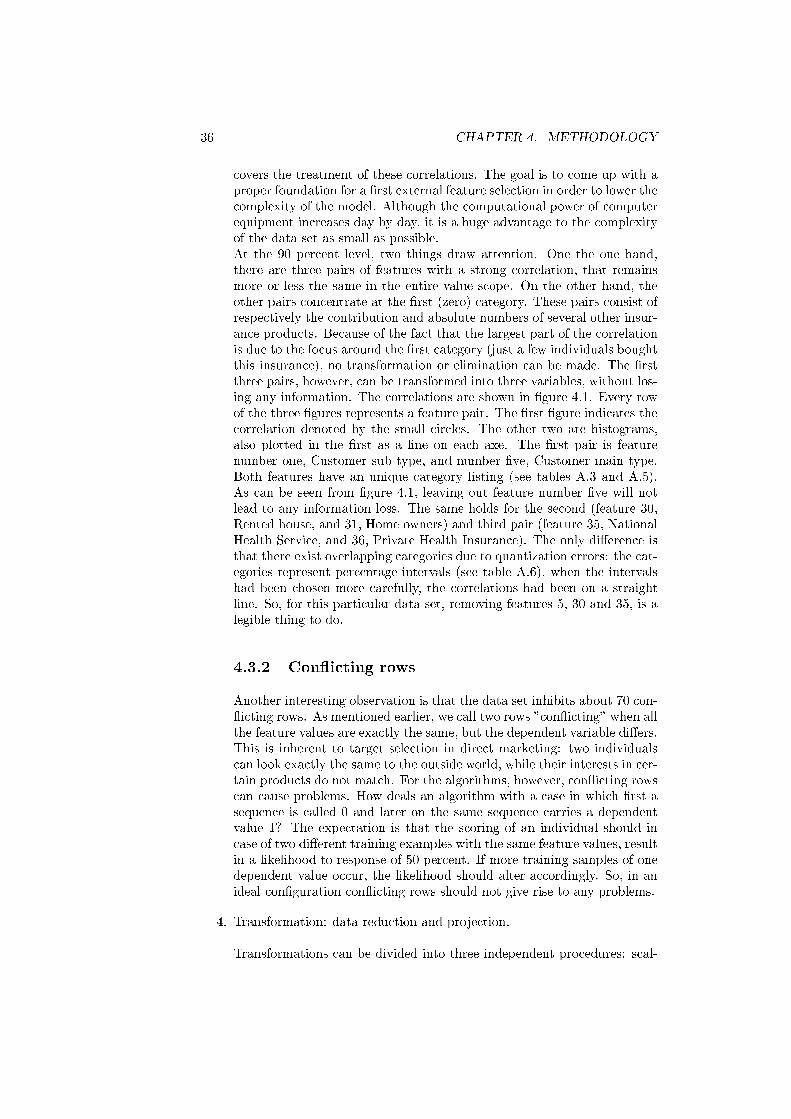
36 CHAPTER 4. METHODOLOGY
covers the treatment of these correlations. The goal is to come up with a
proper foundation for a �rst external feature selection in order to lower the
complexity of the model. Although the computational power of computer
equipment increases day by day, it is a huge advantage to the complexity
of the data set as small as possible.
At the 90 percent level, two things draw attention. One the one hand,
there are three pairs of features with a strong correlation, that remains
more or less the same in the entire value scope. On the other hand, the
other pairs concentrate at the �rst (zero) category. These pairs consist of
respectively the contribution and absolute numbers of several other insur-
ance products. Because of the fact that the largest part of the correlation
is due to the focus around the �rst category (just a few individuals bought
this insurance), no transformation or elimination can be made. The �rst
three pairs, however, can be transformed into three variables, without los-
ing any information. The correlations are shown in �gure 4.1. Every row
of the three �gures represents a feature pair. The �rst �gure indicates the
correlation denoted by the small circles. The other two are histograms,
also plotted in the �rst as a line on each axe. The �rst pair is feature
number one, Customer sub type, and number �ve, Customer main type.
Both features have an unique category listing (see tables A.3 and A.5).
As can be seen from �gure 4.1, leaving out feature number �ve will not
lead to any information loss. The same holds for the second (feature 30,
Rented house, and 31, Home owners) and third pair (feature 35, National
Health Service, and 36, Private Health Insurance). The only di�erence is
that there exist overlapping categories due to quantization errors: the cat-
egories represent percentage intervals (see table A.6), when the intervals
had been chosen more carefully, the correlations had been on a straight
line. So, for this particular data set, removing features 5, 30 and 35, is a
legible thing to do.
4.3.2 Con icting rows
Another interesting observation is that the data set inhibits about 70 con-
icting rows. As mentioned earlier, we call two rows "con icting" when all
the feature values are exactly the same, but the dependent variable di�ers.
This is inherent to target selection in direct marketing: two individuals
can look exactly the same to the outside world, while their interests in cer-
tain products do not match. For the algorithms, however, con icting rows
can cause problems. How deals an algorithm with a case in which �rst a
sequence is called 0 and later on the same sequence carries a dependent
value 1? The expectation is that the scoring of an individual should in
case of two di�erent training examples with the same feature values, result
in a likelihood to response of 50 percent. If more training samples of one
dependent value occur, the likelihood should alter accordingly. So, in an
ideal con�guration con icting rows should not give rise to any problems.
4. Transformation: data reduction and projection.
Transformations can be divided into three independent procedures: scal-

4.3. TARGET SELECTION BY KDD 37
ing, feature selection and the treatment of di�erent kind of variables (see
section 2.2.1). All three are addressed individually.
4.3.3 Scaling
Some algorithms use in their internal feature selection the so-called T-test.
For these algorithms a normalization is required. The T-test is used to
investigate whether a calculated coeÆcient signi�cantly di�ers from zero.
If no scaling is conducted, features with a large value scale will tend to be
more signi�cant than attributes with a modest scale. Therefore, all the
variables are scaled to zero mean and variance one, a commonly applied
transformation.
Because the tendency is that the con�guration that probably performs best
is made up of several algorithms, this scaling is applied because no harm
is done (values still keep their underlying relations) and the calculations
are easy and carried out in a split-second.
4.3.4 Feature selection
The three features which can be excluded according to their strong cor-
relation with other features (section 4.3.1) can be excluded here as an
external selection. Some con�gurations make use of external feature se-
lection, others use internal feature selection, which actually is nothing
more than external selection carried out a number of times in a loop.
4.3.5 Di�erent types of variables
The data set has four types of variables: 62 categorical, 21 continuous,
2 nominal and one binary attribute. The categorical can be treated as
continuous and the binary attribute is the dependent variable. The two
features to worry about are number 1, customer subtype, and number 5,
customer main type. As found in section 4.3.1, these two features have
a very large correlation. Since feature number �ve can be excluded, one
nominal predictor is left. There are a few options how to deal with this
predictor. The simplest one is to leave it out, but we will see that this is
one of the more important predictors. Another option is to transform the
nominal values to continuous ones, but this adds new relations between
the nominal feature predicates. This does not have to be a enormous prob-
lem, but every transformation can be justi�ed. The approach we choose,
depends on our faith in the expertise of the people responsible for con-
structing the category listing. Each value is transformed to its place in the
list. So, "stable family" become 10 and "mixed rurals" closes the listing
with 41. Whether this transformation can be justi�ed, becomes clear in
chapter 5, where the results are presented.
If one has to build its own nominal category list, the aim has to be to estab-
lish some kind of ordinal sequence, if possible. With a listing as customer
sub type, one could think of a list increasing in social status. Although
the subdivision always stays arbitrarily, this approach is better then just
38 CHAPTER 4. METHODOLOGY
transforming the value according to, for instance, their appearance in the
alphabet.
5. Matching the goals of the KDD process to a particular data mining method.
The goal of this KDD process is to predict which customers are likely
to buy a caravan policy.
6. Choosing the data mining algorithm(s).
The mining algorithms used in this these are linear and logistic regression,
Chaid, Neural Networks and a fuzzy modeling technique. Each algorithm
is fully described in chapter 3.
7. Data mining: searching for patterns of interest in a particular representa-
tional form.
The mining of the algorithms consist of two di�erent phase in this thesis
work. The �rst phase consist of the �ve stand-alone algorithms in their
most optimized con�gurations. The second phase is the introduction of
the combinations which uses some results from the �rst phase.
4.3.6 Combining the algorithms
The �ve mining algorithms described in chapter 3 all have di�erent back-
grounds and constrains. This statement is intuitive and the second foun-
dation for the combining is a practical re ection: all algorithms roughly
consist of two major components; one which accounts for the feature selec-
tion and another that scores the customers according to their likelihood of
response. Although some algorithms execute both tasks in the same com-
putational procedure, every algorithm can be added an external feature
selection. Magidson [16] reported that selecting features using Chaid and
scoring by logit is a powerful combination. This procedure can be applied
in general: one con�guration selects the important features and a second
con�guration uses these features for the client scoring. Because there are
usually a lot of attributes in a direct marketing database, feature selection
is necessary to identify the important features. Every algorithm selecting
features, however, su�ers from algorithm speci�c assumptions: normally
distributed data, for instance. Because the total number of attributes is
high, several feature selecting algorithms can be applied. These rarely
come up with exactly the same feature subsets. If we assume that we
have suÆcient feature selecting algorithms (a domain expert can also be
an "algorithm"), we have the availability of several feature subsets which
inhibit relevant attributes to the target selection problem.
The next question is how to assign a score to each client, given these
feature subsets. One option is to construct one large feature set, with
all features present in the feature sets given by the feature selecting algo-
rithms. The disadvantage of this approach is that the unique structures of
the former feature sets are lost. Another related problem, is what con�g-
uration should be used to score the clients only using the features present

4.3. TARGET SELECTION BY KDD 39
in this set? Other options of combining feature sets before scoring the
prospects will have to conquer the same problems. The solution is simple:
score all feature sets separately by algorithms which are known or expected
to do well. This results in di�erent scores for each client in the database.
Assign all scores a weight depending on the expected performance by the
speci�c con�guration and multiply the scores with these weights before
adding them up resulting in a �nal client score.
Mathematically expressed, if we have a data set with N customers andK
attributes, and R feature selecting algorithms (FSAr) selecting R fea-
ture subsets FTr with k(r) < K features each, we also need R scoring
algorithms (SAr) giving each customer n � N a score scnr and the
total score for client n is given by:
SCn =Xr
�rscnr; (4.2)
in which �r is the weight factor for scoring algorithm r. In the ideal case,
the sum of these weights equals 1:Xr
�r = 1: (4.3)
There are three special cases:
(a) The feature selecting algorithm can be the same for all R scoring al-
gorithms, hence the same feature (sub)set is used for di�erent scoring
con�gurations. Example: �nding the optimal number of neurons in
the hidden layer of a Arti�cial Neural Network.
(b) The scoring algorithm can be the same for all R feature selecting
algorithms. Example: �nding the best feature subset for logistic
regression as scoring algorithm.
(c) The feature selecting algorithm is absent or the same as the scoring
algorithm and R equals one. This is target selection in the "old-
fashioned" way.
Next to the special cases, by manipulating the weight factors, one can build
an algorithm selecting{target selection con�guration. The total method is
summarized in the owchart given in AD1. The only problem left is how
to determine appropriate values for the �'s.
Setting the Weight Factors
The weight factor gives a con�guration a degree of importance with respect
to the other con�gurations used in a combination. Di�erent con�gurations
rarely come up with scores on the same value scale. So, the second task
of the weight factor is transforming the scores given by the di�erent con-
�gurations to the same scale. In order to establish a proper distinction
between both tasks the weight factor can be split up into two factors: one
representing the relative degree of importance and the other to scale the
scores.
�r = �r r (4.4)

40 CHAPTER 4. METHODOLOGY
In equation 4.4 the weight factor � is split into �, which represents the
degree of importance and which is the scaling factor. The latter can
easily be computed:
r =NPn scnr
(4.5)
Four di�erent sets of weight factors are used. The �rst, straightforward,
way is to give all �'s the same value: 1=R. The second way is to set
all �r to 1 and calculate the r 's according to equation 4.5. In order to
satisfy (4.3), the resulting scores SCn can be divided by the total sum of
the scale factors, such that new scaled SCn values are obtained:
SCn;new =SCn;oldP
r r
(4.6)
The third way to determine the weight factors is to apply a procedure
which optimizes the �'s, such as linear regression. The drawback of this
approach is that some weight factors can become negative. This can be
prevented by using a linear regression with positive coeÆcients.The �nal
way to set the � weights is based on domain expertise. A domain expert
can be someone with expert knowledge of or intensive experience with the
algorithms, the (kind of) data set or, ideally, both. If there are indications
that one algorithm performs better on a data set than others, the weight
factor � for this algorithm can be increased accordingly.
4.3.7 Test structure
We assume that we have the availability of a train and a score set. The �rst
is used for training and a �rst validation, the second for a out-of-sample
test. In order to raise the generalizing power of the model, the train set
is randomly divided into three sets, such that the overall percentage of
respondents was kept. Two sets are, in turn, used for training and the
third as a �rst validation. Finally, a fourth model is built by adding all
three sets. By doing so, four di�erent models are used, which on turn
can be treated as one model by assigning each model weights. In AD2
the procedure is drawn. The models mentioned in this �gure represent
stand-alone algorithms or the con�guration of AD1, the combination of
several algorithms.
The performance measures on the �rst validation sets ("val" 1 to 3) are
not numerically given in this thesis. The reason follows in section 5.1.
They can, however, be a �rst indication which model trained on the cross
sets performs best. The performances that we will report are labeled
"score" 1 to 3, the performance of the three models based on the cross
sets, "score" 4, the performance of the model based on the entire train
set and "avg score", the three cross models added up in the same way we
combine di�erent algorithms.
8. Interpretation of patterns found, and possibly return to any of the steps
1-7.
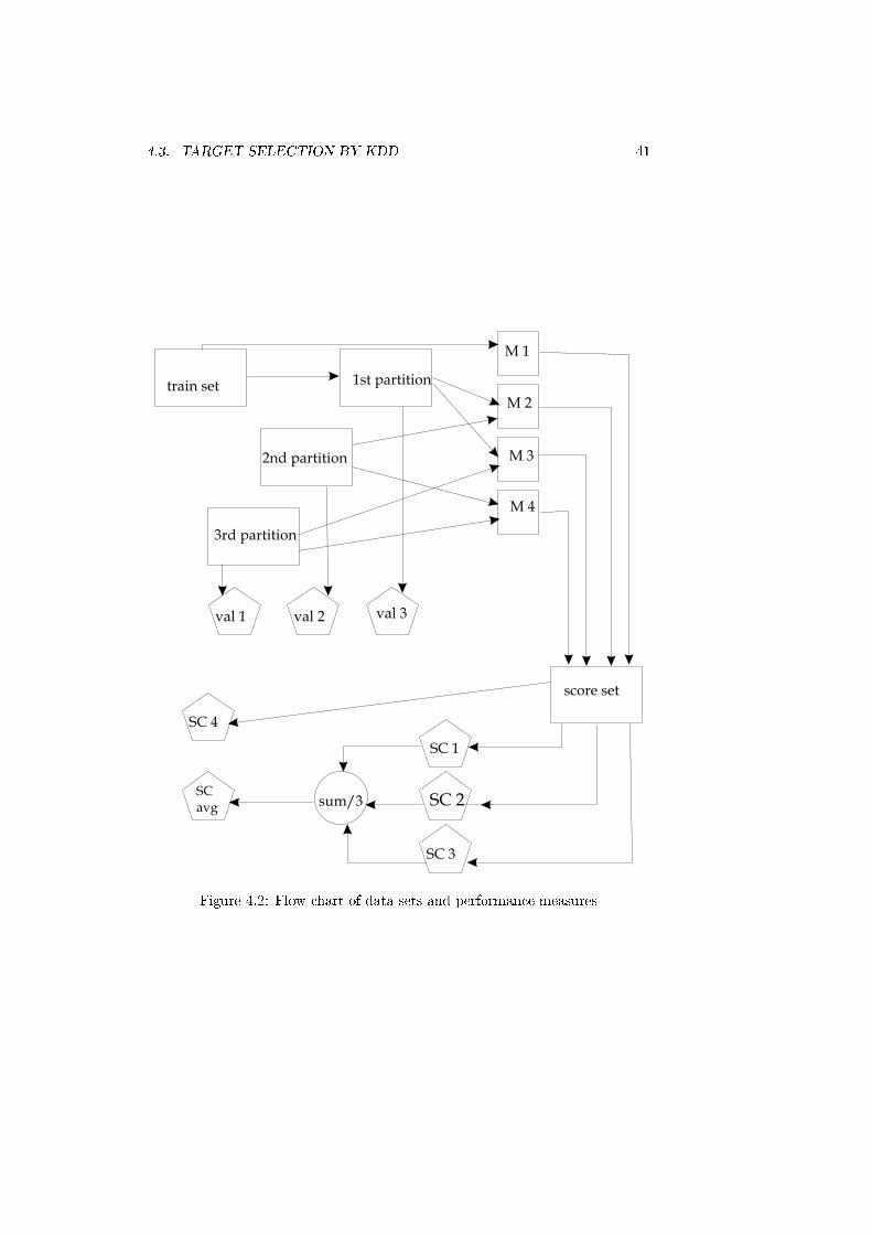
4.3. TARGET SELECTION BY KDD 41
train set 1st partition
2nd partition
3rd partition
M 1
M 2
M 3
M 4
score set
SC 1
SC 2
SC 3
sum/3
SC 4
SCavg
val 1 val 2 val 3
Figure 4.2: Flow chart of data sets and performance measures
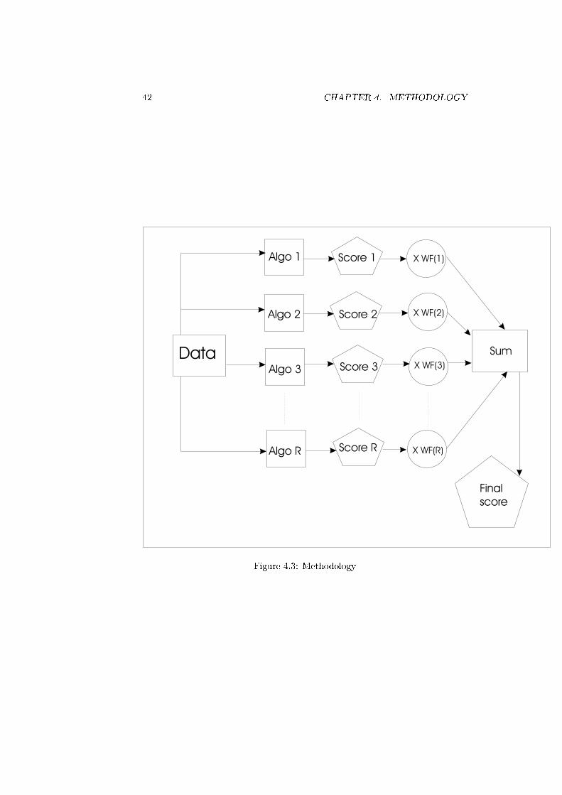
42 CHAPTER 4. METHODOLOGY
Data
Algo 1
Algo 2
Algo 3
Algo R
Score 1
Score 2
Score 3
Score R
Sum
Final
score
X WF(1)
X WF(2)
X WF(3)
X WF(R)
Figure 4.3: Methodology

4.3. TARGET SELECTION BY KDD 43
The interpretation of the eventual feature set on the basis of the origi-
nal CoIL assignment is part of chapter 5.
9. Consolidating the discovered knowledge: incorporating this knowledge in
another system for further action.
The systems in which the deducted knowledge is incorporated are on the
one hand the unseen data of the third subset in the 3 way cross validation.
On the other hand all �nal con�gurations are used to predict likelihood
of response of the individuals in the "score" set of the CoIL challenge.
Results on this set are compared to previous obtained results by the con-
testants of the CoIL challenge and can be found in chapter 5.

44 CHAPTER 4. METHODOLOGY

Chapter 5
Results
In this chapter the results of the methodology presented in the previous chapter
are reported for the data set which was also introduced and investigated in
chapter 4. As mentioned earlier, the analysis of direct marketing campaigns
entails two stages. First, feature selection must determine the variables that are
relevant for the speci�c target selection problem. second, the rules for selecting
the customers should be determined, given the relevant features. This stages is
referred to as client scoring. In the KDD cycle described in chapter 2, external
feature selection is part of step 4, and the internal feature selection occurs as a
loop over step 4 to 8.
This chapter is divided into three sections: in section 5.1 the results for the
optimal con�guration for each algorithm used stand-alone are presented and
discussed, in section 5.2 the same goes for the combinations and �nally, in
section 5.3, the results of the previous two sections are compared to the results
of the best CoIL submissions.
5.1 Stand-alone algorithms
Linear regression
If we use all features and use linear regression to score all clients, we obtain
the gain charts drawn in �gure 5.1. The corresponding number of correctly
predicted respondents in the �rst ordered 20 % of all clients can be found in
table 5.1.
The second column (labeled "VAL") in this table gives the values of the respon-
set VAL SCORE
ran 23 48
1st 61 121
2nd 57 110
3rd 57 115
tot 200 118
avg - 115
Table 5.1: CPM values for linear regression with all features
45

46 CHAPTER 5. RESULTS
0 50 1000
20
40
60
80
100first crossvalidation
customers mailed [%]
resp
onde
nts
targ
eted
[%]
Train data First validationScore data
0 50 1000
20
40
60
80
100second crossvalidation
customers mailed [%]
resp
onde
nts
targ
eted
[%]
0 50 1000
20
40
60
80
100third crossvalidation
customers mailed [%]
resp
onde
nts
targ
eted
[%]
0 50 1000
20
40
60
80
100entire TIC trainset
customers mailed [%]
resp
onde
nts
targ
eted
[%]
Figure 5.1: Gain chart for linear regression using all features

5.1. STAND-ALONE ALGORITHMS 47
dents in that part of the train set which has not been used to train the model.
The exception is the model which has been trained and validated on the whole
train set (tot). The second row gives the number of respondents which would
have been correctly identi�ed by random mailing. The other rows represent the
models based on the three cross validation sets, the total train set and a model
based on all three cross sets (avg). This fourth model is trained and (at �rst)
validated on the entire train set. In order to calculate the gain, the number of
the random mailing has to be multiplied by three. The highest score on the
score set is 121, based on the model trained on the �rst cross validation. This is
a gain of 252 % compared to random mailing. Despite of the fact that this result
is a good one (see section 5.2), how can we predict that the model based on the
�rst cross validation is the best? One way is pick the model that scores best on
the "VAL" sets. This approach has a few disadvantages: the �rst problem is
how the fourth model which is based on the entire train set, has to be compared
to the other ones. We could divided the "VAL" value by three, but it is obvious
that this value is not representative because the validation samples are the same
as the train samples. Another option is to discard the fourth model, but as we
will see, some models based on the entire train set prove to be the best ones. A
third way to overcome this problem is to adopt a new client score based on the
client scores given by the models based on the three cross validation sets in the
same way as combining the models is suggested in section 4.3.6. The weights
are set to 1/3. The resulting number (avg) of respondents for the score set is
equal to 115. We believe this is the best way to score clients in real life, although
there will be some exceptions. To test this hypothesis, we shall give all results
in the same format as table 5.1 without giving the "VAL" values because they
do not help in deciding whether to rely on the "tot" or "avg" model.
External feature selection based on correlation is mentioned in section 3.1. If we
adopt the rule (equation 3.8) that only includes those features with a absolute
correlation twice or large then the mean absolute correlation to the dependent
attribute of all independent features, the feature set obtained is given in table
5.2 for the tic data set. We shall refer to this feature set as correlation fea-
Table 5.2: Features with large correlation to Caravan policies owners
No Name No Name
16 High education level 59 Contribution �re policies
18 Lower level education 61 Contribution boat policies
42 Average income 65 Number of pr. 3rd party insurance
43 Purchasing power class 68 Number of car policies
44 Contribution pr. 3rd party 82 Number of bicycle policies
47 Contribution car policies
tures A. If we adopt a second rule which excludes features that have a large
correlation (> 90 %) to each other we obtain the same feature set as listed in
table 5.2 without features 61, 65 and 68. This set is named correlation features
B. Linear regression on the correlation feature subset A results in CPM's (see
section 4.2) which are given in table 5.3. In this table the di�erent values are
given for all �ve di�erent models. These values will act as benchmark for the
other con�gurations.
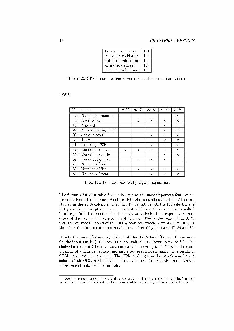
48 CHAPTER 5. RESULTS
1st cross validation 111
2nd cross validation 112
3rd cross validation 112
entire tic data set 110
avg cross validation 110
Table 5.3: CPM values for linear regression with correlation features
Logit
No name 98 % 90 % 85 % 80 % 75 %
2 Number of houses x
4 Average age x x x x
10 Married x x
22 Middle management x x
28 Social class C x x x
32 1 car x x
41 Income > 123K x x x
47 Contribution car x x x x x
55 Contribution life x x
59 Contribution �re x x x x x
76 Number of life x
80 Number of �re x x x x x
82 Number of boat x x x
Table 5.4: Features selected by logit as signi�cant
The features listed in table 5.4 can be seen as the most important features se-
lected by logit. For instance, 85 of the 100 selections all selected the 7 features
(tabled in the 85 % column): 4, 28, 41, 47, 59, 80, 82. Of the 100 selections, 2
just gave the intercept as single important predictor, these selections resulted
in an especially bad (but not bad enough to activate the escape ag 1) con-
ditioned data set, which caused this di�erence. This is the reason that 98 %
features are listed instead of the 100 % features, which is empty. One way or
the other, the three most important features selected by logit are: 47, 59 and 80.
If only the seven features signi�cant at the 85 % level (table 5.4) are used
for the input (scaled), this results in the gain charts shown in �gure 5.2. The
choice for the best 7 features was made after inspecting table 5.4 with the com-
bination of a high percentage and just a few predictors in mind. The resulting
CPM's are listed in table 5.5. The CPM's of logit on the correlation feature
subset of table 5.2 are also listed. These values are slightly better, although the
improvement hold for all train sets.
1Some selections are extremely bad conditioned, in these cases the "escape ag" is acti-
vated; the current run is terminated and a new initialization, e.g. a new selection is used
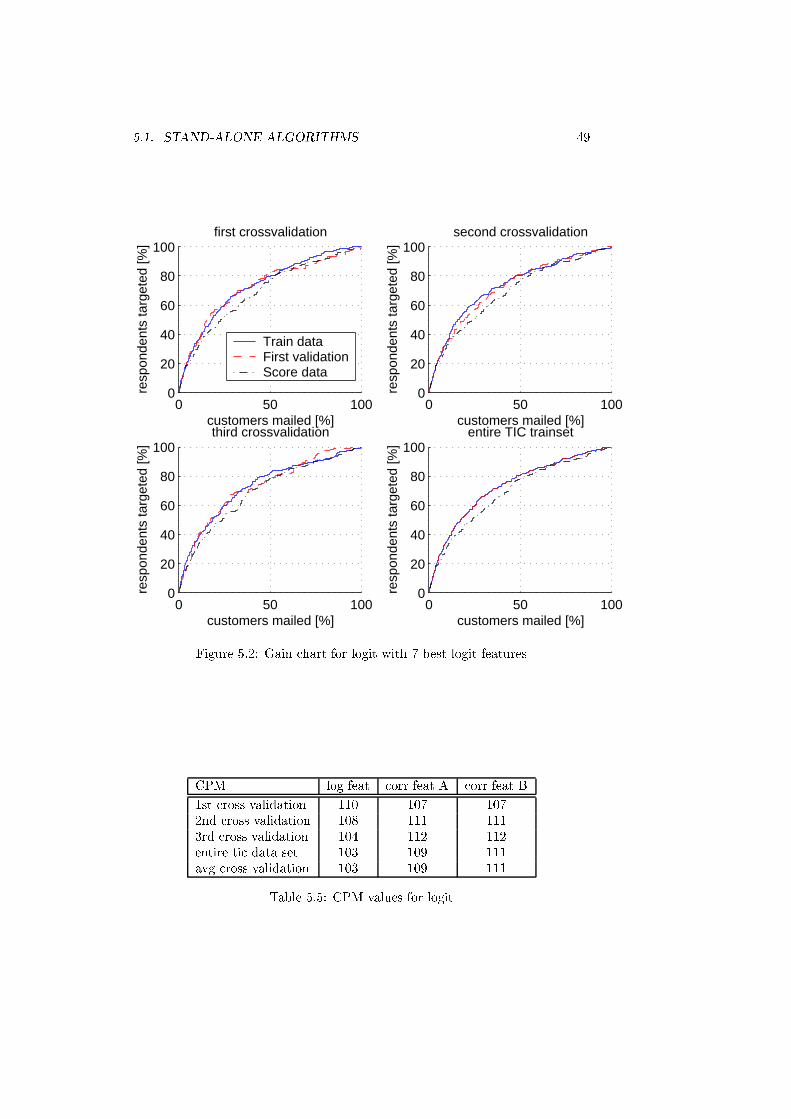
5.1. STAND-ALONE ALGORITHMS 49
0 50 1000
20
40
60
80
100first crossvalidation
customers mailed [%]
resp
onde
nts
targ
eted
[%]
Train data First validationScore data
0 50 1000
20
40
60
80
100second crossvalidation
customers mailed [%]
resp
onde
nts
targ
eted
[%]
0 50 1000
20
40
60
80
100third crossvalidation
customers mailed [%]
resp
onde
nts
targ
eted
[%]
0 50 1000
20
40
60
80
100entire TIC trainset
customers mailed [%]
resp
onde
nts
targ
eted
[%]
Figure 5.2: Gain chart for logit with 7 best logit features
CPM log feat corr feat A corr feat B
1st cross validation 110 107 107
2nd cross validation 108 111 111
3rd cross validation 104 112 112
entire tic data set 103 109 111
avg cross validation 103 109 111
Table 5.5: CPM values for logit
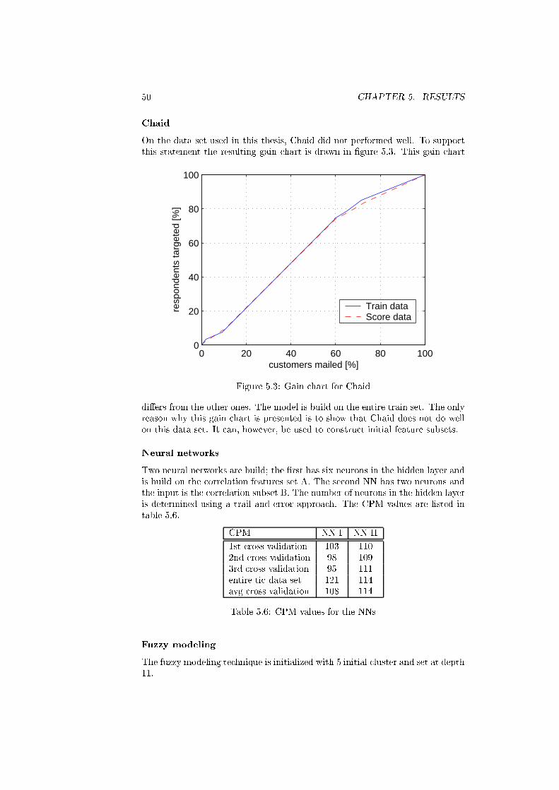
50 CHAPTER 5. RESULTS
Chaid
On the data set used in this thesis, Chaid did not performed well. To support
this statement the resulting gain chart is drawn in �gure 5.3. This gain chart
0 20 40 60 80 1000
20
40
60
80
100
customers mailed [%]
resp
onde
nts
targ
eted
[%]
Train dataScore data
Figure 5.3: Gain chart for Chaid
di�ers from the other ones. The model is build on the entire train set. The only
reason why this gain chart is presented is to show that Chaid does not do well
on this data set. It can, however, be used to construct initial feature subsets.
Neural networks
Two neural networks are build; the �rst has six neurons in the hidden layer and
is build on the correlation features set A. The second NN has two neurons and
the input is the correlation subset B. The number of neurons in the hidden layer
is determined using a trail and error approach. The CPM values are listed in
table 5.6.
CPM NN I NN II
1st cross validation 103 110
2nd cross validation 98 109
3rd cross validation 95 111
entire tic data set 121 114
avg cross validation 108 114
Table 5.6: CPM values for the NNs
Fuzzy modeling
The fuzzy modeling technique is initialized with 5 initial cluster and set at depth
11.
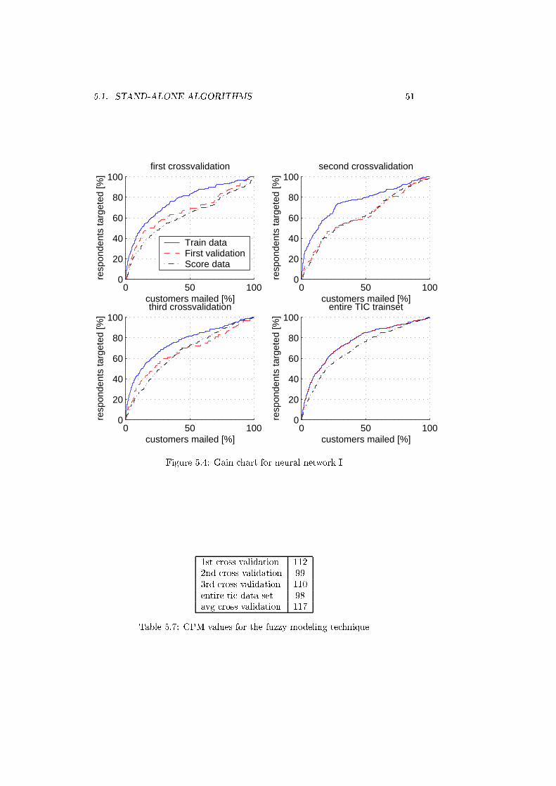
5.1. STAND-ALONE ALGORITHMS 51
0 50 1000
20
40
60
80
100first crossvalidation
customers mailed [%]
resp
onde
nts
targ
eted
[%]
Train data First validationScore data
0 50 1000
20
40
60
80
100second crossvalidation
customers mailed [%]
resp
onde
nts
targ
eted
[%]
0 50 1000
20
40
60
80
100third crossvalidation
customers mailed [%]
resp
onde
nts
targ
eted
[%]
0 50 1000
20
40
60
80
100entire TIC trainset
customers mailed [%]
resp
onde
nts
targ
eted
[%]
Figure 5.4: Gain chart for neural network I
1st cross validation 112
2nd cross validation 99
3rd cross validation 110
entire tic data set 98
avg cross validation 117
Table 5.7: CPM values for the fuzzy modeling technique
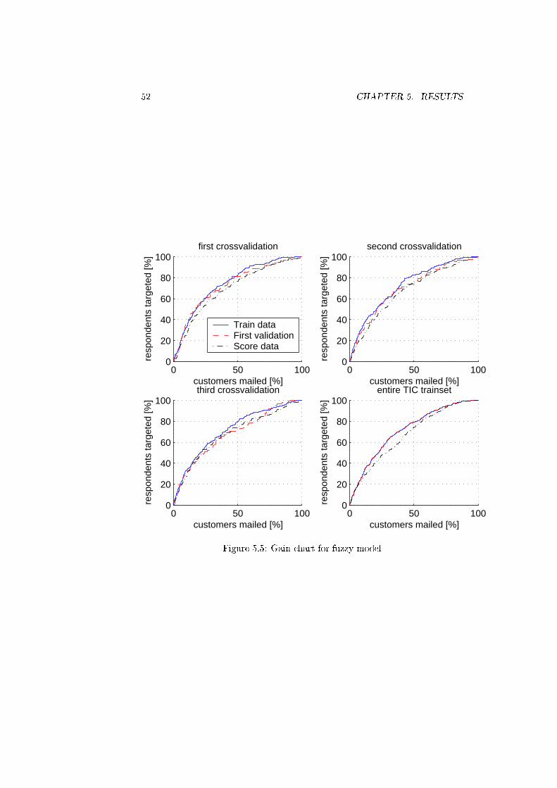
52 CHAPTER 5. RESULTS
0 50 1000
20
40
60
80
100first crossvalidation
customers mailed [%]
resp
onde
nts
targ
eted
[%]
Train data First validationScore data
0 50 1000
20
40
60
80
100second crossvalidation
customers mailed [%]
resp
onde
nts
targ
eted
[%]
0 50 1000
20
40
60
80
100third crossvalidation
customers mailed [%]
resp
onde
nts
targ
eted
[%]
0 50 1000
20
40
60
80
100entire TIC trainset
customers mailed [%]
resp
onde
nts
targ
eted
[%]
Figure 5.5: Gain chart for fuzzy model
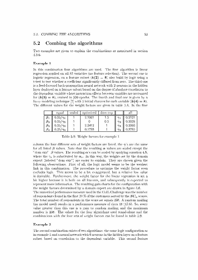
5.2. COMBING THE ALGORITHMS 53
5.2 Combing the algorithms
Two examples are given to explain the combinations as mentioned in section
4.3.6.
Example 1
In this combination four algorithms are used. The �rst algorithm is linear
regression applied on all 85 variables (no feature selection). The second one is
logistic regression, on a feature subset (k(2) = 8) also build by logit using a
t-test to test whether a coeÆcient signi�cantly di�ered from zero. The third one
is a feed-forward back-propagation neural network with 2 neurons in the hidden
layer deployed on a feature subset based on the degree of absolute correlation to
the dependent variable where interaction e�ects between variables are accounted
for (k(3) = 8), trained in 500 epochs. The fourth and �nal one is given by a
fuzzy modeling technique [7] with 5 initial clusters for each variable (k(4) = 8).
The di�erent values for the weight factors are given in table 5.8. In the �rst
equal scaled optimized dom exp all
�1 0.25/ 1 1 2.1061 1.5 1 0.2131
�2 0.25/ 2 1 0 0.5 2 0.2038
�3 0.25/ 3 1 2.3412 1 3 0.2066
�4 0.25/ 4 1 0.1793 1 4 0.3765
Table 5.8: Weight factors for example 1
column the four di�erent sets of weight factors are listed, the 's are the same
for all listed � values. Note that the resulting � values are scaled except the
"dom exp" -� values. The resulting �'s can be scaled by applying equation 4.5,
where the r is substituted by �r . In this way, the weights set by the domain
expert (labeled "dom exp") are easier to explain. They are chosen given the
following observations. First of all, the logit model seems to be the weakest
link in this combination. The procedure to optimize the weight factor even
excludes logit. This seems to be a bit exaggerated, but a relative low value
is desirable. Furthermore, the weight factor for the linear regression is set a
bit higher because it is built on all features, and subsequently is expected to
represent more information. The resulting gain charts for the con�guration with
the weight factors determined by a domain expert are drawn in �gure 5.6.
The numerical performance measure used in the CoIL Challenge was the number
of respondents found in the �rst 20 % of the customers sorted by the SCn scores.
The total number of respondents in the score set equals 238. A random mailing
(no model used) results in a performance measure of circa 48 (47.6). So, every
value greater than this one is a gain to random mailing and the maximum
number is 238. The values for the four algorithms used stand-alone and the
combinations with the four sets of weight factors can be found in table 5.9.
Example 2
The second combination exists of two algorithms: the same logit con�guration as
in example 1 and a neural network with 6 neurons in the hidden layer on a feature
subset based on correlation to the dependent variable. This second feature
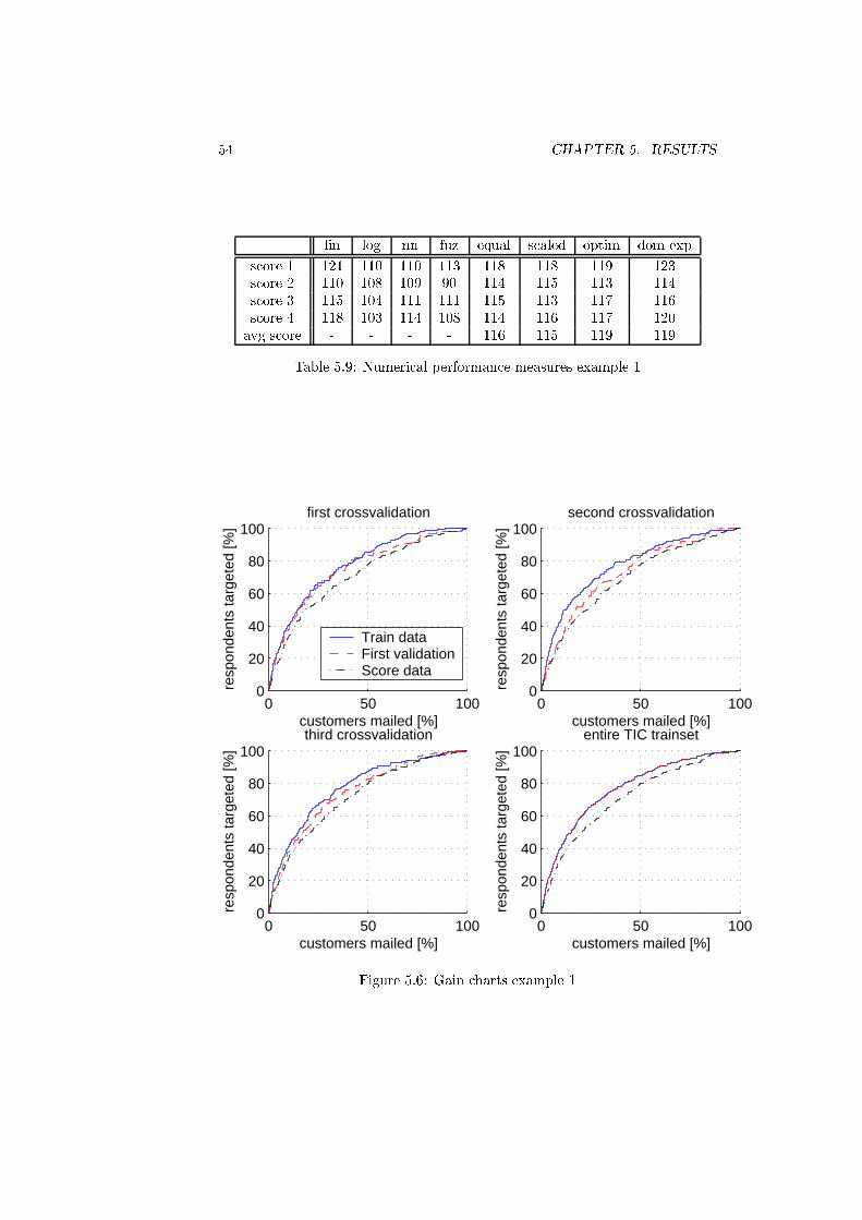
54 CHAPTER 5. RESULTS
lin log nn fuz equal scaled optim dom exp
score 1 121 110 110 113 118 118 119 123
score 2 110 108 109 90 114 115 113 114
score 3 115 104 111 111 115 113 117 116
score 4 118 103 114 108 114 116 117 120
avg score - - - - 116 115 119 119
Table 5.9: Numerical performance measures example 1
0 50 1000
20
40
60
80
100first crossvalidation
customers mailed [%]
resp
onde
nts
targ
eted
[%]
Train data First validationScore data
0 50 1000
20
40
60
80
100second crossvalidation
customers mailed [%]
resp
onde
nts
targ
eted
[%]
0 50 1000
20
40
60
80
100third crossvalidation
customers mailed [%]
resp
onde
nts
targ
eted
[%]
0 50 1000
20
40
60
80
100entire TIC trainset
customers mailed [%]
resp
onde
nts
targ
eted
[%]
Figure 5.6: Gain charts example 1
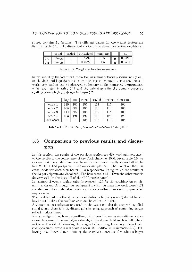
5.3. COMPARISON TO PREVIOUS RESULTS AND DISCUSSION 55
subset contains 11 features. The di�erent values for the weight factors are
listed in table 5.10. The dissentient choice of the domain expertise weights can
equal scaled optimized dom exp all
�1 0.5/ 1 1 1.3897 0.5 1 0.6456
�2 0.5/ 2 1 0.2929 1.5 2 0.3544
Table 5.10: Weight factors for example 2
be explained by the fact that this particular neural network performs really well
on the data and logit does less, as can be seen in example 1. The combination
works very well as can be observed by looking at the numerical performances
which are listed in table 5.11 and the gain charts for the domain expertise
con�guration which are drawn in �gure 5.7.
log nn equal scaled optim dom exp
score 1 110 103 105 107 115 104
score 2 108 98 106 106 110 104
score 3 114 95 106 108 114 106
score 4 103 121 122 115 123 125
avg score - - 108 108 115 108
Table 5.11: Numerical performance measures example 2
5.3 Comparison to previous results and discus-
sion
In this section, the results of the previous section are discussed and compared
to the results of the contestants of the CoIL challenge 2000. From table 5.9, we
can see that the model based on the entire train set correctly scores 120 in the
�rst 20 % ranked prospects in the out-of-sample test. The model on the �rst
cross validation does even better: 123 respondents. In �gure 5.8 the results of
the 43 participants are visualized. The best score is 121. Even the other models
do very well (in the best 5% of the CoIL participants).
In example 2 even a higher value is reached: 125 for the combination on the
entire train set. Although the con�guration with the neural network scored 121
stand-alone, the combination with logit adds another 4 successfully predicted
respondents.
The models build on the three cross validation sets ("avg score") do not have a
better result than the combinations on the entire train set.
Although some con�gurations used in the two examples do very well applied
stand-alone, there is a signi�cant gain in using approach of combining target
selection algorithms.
Every con�guration, hence algorithm, introduces its own systematic errors be-
cause the assumptions underlying the algorithm do not hold to their full extend
in the real world. Optimizing the weight factors using linear regression treats
each systematic error as a random error in the addition sum (equation 4.2). Fol-
lowing this observation, optimizing the weights is more justi�ed when a larger
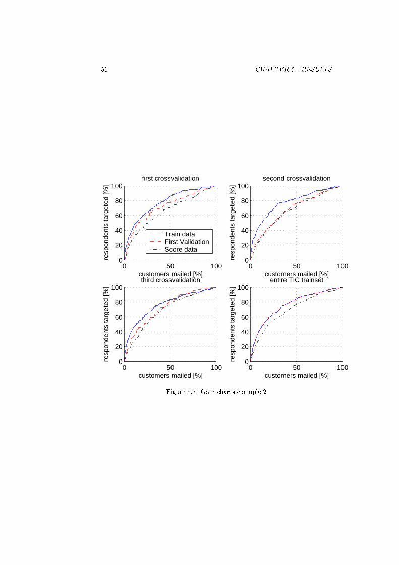
56 CHAPTER 5. RESULTS
0 50 1000
20
40
60
80
100first crossvalidation
customers mailed [%]
resp
onde
nts
targ
eted
[%]
Train data First ValidationScore data
0 50 1000
20
40
60
80
100second crossvalidation
customers mailed [%]
resp
onde
nts
targ
eted
[%]
0 50 1000
20
40
60
80
100third crossvalidation
customers mailed [%]
resp
onde
nts
targ
eted
[%]
0 50 1000
20
40
60
80
100entire TIC trainset
customers mailed [%]
resp
onde
nts
targ
eted
[%]
Figure 5.7: Gain charts example 2
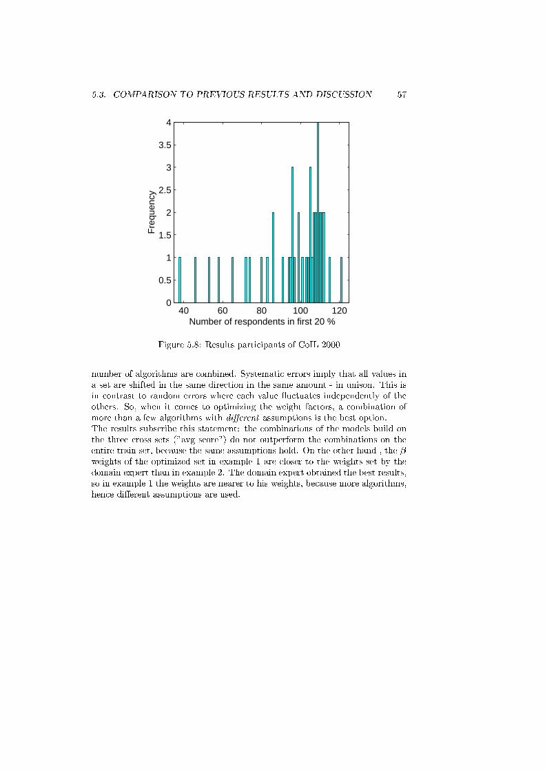
5.3. COMPARISON TO PREVIOUS RESULTS AND DISCUSSION 57
40 60 80 100 1200
0.5
1
1.5
2
2.5
3
3.5
4
Number of respondents in first 20 %
Fre
quen
cy
Figure 5.8: Results participants of CoIL 2000
number of algorithms are combined. Systematic errors imply that all values in
a set are shifted in the same direction in the same amount - in unison. This is
in contrast to random errors where each value uctuates independently of the
others. So, when it comes to optimizing the weight factors, a combination of
more than a few algorithms with di�erent assumptions is the best option.
The results subscribe this statement: the combinations of the models build on
the three cross sets ("avg score") do not outperform the combinations on the
entire train set, because the same assumptions hold. On the other hand , the �
weights of the optimized set in example 1 are closer to the weights set by the
domain expert than in example 2. The domain expert obtained the best results,
so in example 1 the weights are nearer to his weights, because more algorithms,
hence di�erent assumptions are used.

58 CHAPTER 5. RESULTS

Chapter 6
Conclusions and
Recommendations
The conclusions of this thesis project are given in this section, followed by some
recommendations for future research.
Conclusions
Despite the fact that many algorithms are developed for the purpose of target
selection, no universal algorithm exist. The strength of the approach presented
in this thesis is that the structure and speci�c characteristics of each feature sub-
set are maintained and scored individually. If proper action is taken to prevent
over-training in building the algorithms, combining them will not introduce any
kind of over-training. The quality of the train samples are equally important in
preventing over-training. Spurious relations can be found, especially in case of
a large number of algorithms in a combination.
By adequately combining the scores, results are achieved out-performing all par-
ticipants in the CoIL challenge 2000. The best results are obtained by using
the weights chosen by a domain expert. If such a person is not available, the
best way seems to be optimizing the weights using a linear regression method
with positive coeÆcients. A fairly large number of algorithms with di�erent
assumptions is needed for adequately optimized weights.
Di�erent kinds of variables do not need special treatments. Except for the
nominal variables which have to be transformed adding new non-existing rela-
tion between the variables values.
NNs need scaling to operate and feature selection by logit requires scaling. Lin-
ear regression, Chaid and the fuzzy modeling technique do not need scaling of
the inputs.
Experiments on the data set pointed out that the NN performs best, followed
closely by linear regression. The fuzzy modeling technique and logit did a bit
less. Chaid is found to fail on the data set investigated.
Several combinations of the algorithms are proposed, and the combination of
logit and NNs does outperform every contestant of the CoIL challenge. Al-
though the extra gain is marginal in the high cost { high impact environment
59

60 CHAPTER 6. CONCLUSIONS AND RECOMMENDATIONS
every gain increases pro�t.
Recommendations for further research
Further research has to be done to �nd out where the limits of combining algo-
rithms are at. To put in other words, how sensitive this approach is to adding a
large number of di�erent combinations. Another question is how cross validation
could better be integrated in this technique.
Some general recommendations are:
1. The format in which the data set is recorded must be improved. The peo-
ple responsible for the data collection need to contact the ones responsible
for target selection. This could, for instance, prevent quantization errors.
2. Instead of optimizing the algorithms itself, they could be optimized on the
gain chart. For instance, the NN is not updated on the known output,
but by optimizing the gains on the gain chart.
3. Interaction e�ects can be added as extra features. In this way, more
features are present, but perhaps better modelling capabilities introduced.

Appendix A
Tables of the features and
datasets
In this appendix the feature labels with a short describtion are listed in tables
A.1 and A.2.
Next to the feature labels, the di�erent categories, as named in the 'domain'{
column (see tables A.1 and A.2, are given. The �rst category is L0, the customer
sub type categories, see table A.3. This category consist of nominal values, 41
in total. The only other nominal category is L2, as listed in table A.5, and has
eleven di�erent values. As stated in section 4.3.1, the features who use these
two categories have a strong correlation, where L0 is merely more detailed.
Category type L1 (table A.4) contains categorical age values. Category type
L3, percentage and L4 the annual contribution to a certain insurance in Dutch
guilders (see tables A.6 and A.7).
61

62 APPENDIX A. TABLES OF THE FEATURES AND DATASETS
Table A.1: Listing of the attributes 1 to 43
Nr Name Description Domain
1 MOSTYPE Customer subtype see L0
2 MAANTHUI Number of houses 1 to 10
3 MGEMOMV Avg size household 1 to 6
4 MGEMLEEF Avg age see L1
5 MOSHOOFD Customer main type see L2
6 MGODRK Roman catholic see L3
7 MGODPR Protestant
8 MGODOV Other religion
9 MGODGE No religion
10 MRELGE Married
11 MRELSA Living together
12 MRELOV Other relation
13 MFALLEEN Singles
14 MFGEKIND Household without children
15 MFWEKIND Household with children
16 MOPLHOOG High level education
17 MOPLMIDD Medium level education
18 MOPLLAAG Lower level education
19 MBERHOOG High status
20 MBERZELF Entrepreneur
21 MBERBOER Farmer
22 MBERMIDD Middle management
23 MBERARBG Skilled labourers
24 MBERARBO Unskilled labourers
25 MSKA Social class A
26 MSKB1 Social class B1
27 MSKB2 Social class B2
28 MSKC Social class C
29 MSKD Social class D
30 MHHUUR Rented house
31 MHKOOP Home owners
32 MAUT1 1 car
33 MAUT2 2 cars
34 MAUT0 No car
35 MZFONDS National Health Service
36 MZPART Private health insurance
37 MINKM30 Income < 30.000
38 MINK3045 Income 30 to 45.000
39 MINK4575 Income 45 to 75.000
40 MINK7512 Income 75 to 122.000
41 MINK123M Income >123.000
42 MINKGEM Average income
43 MKOOPKLA Purchasing power class
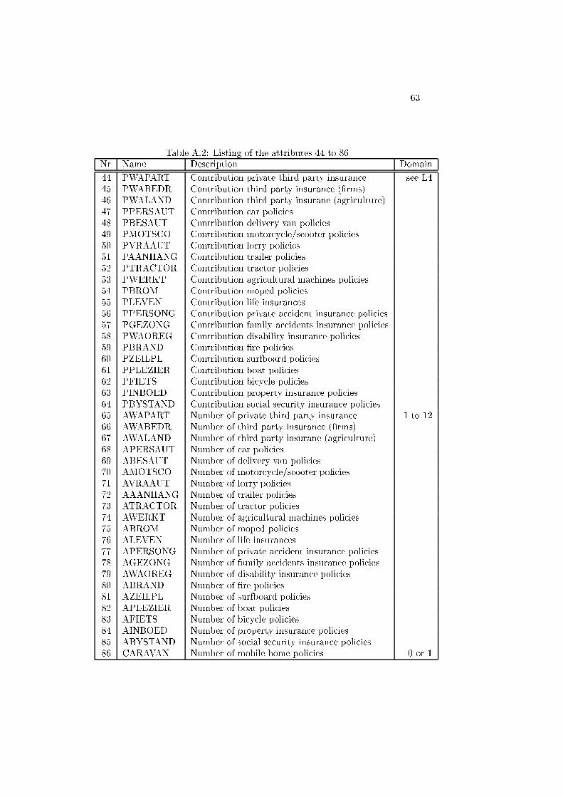
63
Table A.2: Listing of the attributes 44 to 86
Nr Name Description Domain
44 PWAPART Contribution private third party insurance see L4
45 PWABEDR Contribution third party insurance (�rms)
46 PWALAND Contribution third party insurane (agriculture)
47 PPERSAUT Contribution car policies
48 PBESAUT Contribution delivery van policies
49 PMOTSCO Contribution motorcycle/scooter policies
50 PVRAAUT Contribution lorry policies
51 PAANHANG Contribution trailer policies
52 PTRACTOR Contribution tractor policies
53 PWERKT Contribution agricultural machines policies
54 PBROM Contribution moped policies
55 PLEVEN Contribution life insurances
56 PPERSONG Contribution private accident insurance policies
57 PGEZONG Contribution family accidents insurance policies
58 PWAOREG Contribution disability insurance policies
59 PBRAND Contribution �re policies
60 PZEILPL Contribution surfboard policies
61 PPLEZIER Contribution boat policies
62 PFIETS Contribution bicycle policies
63 PINBOED Contribution property insurance policies
64 PBYSTAND Contribution social security insurance policies
65 AWAPART Number of private third party insurance 1 to 12
66 AWABEDR Number of third party insurance (�rms)
67 AWALAND Number of third party insurane (agriculture)
68 APERSAUT Number of car policies
69 ABESAUT Number of delivery van policies
70 AMOTSCO Number of motorcycle/scooter policies
71 AVRAAUT Number of lorry policies
72 AAANHANG Number of trailer policies
73 ATRACTOR Number of tractor policies
74 AWERKT Number of agricultural machines policies
75 ABROM Number of moped policies
76 ALEVEN Number of life insurances
77 APERSONG Number of private accident insurance policies
78 AGEZONG Number of family accidents insurance policies
79 AWAOREG Number of disability insurance policies
80 ABRAND Number of �re policies
81 AZEILPL Number of surfboard policies
82 APLEZIER Number of boat policies
83 AFIETS Number of bicycle policies
84 AINBOED Number of property insurance policies
85 ABYSTAND Number of social security insurance policies
86 CARAVAN Number of mobile home policies 0 or 1

64 APPENDIX A. TABLES OF THE FEATURES AND DATASETS
Table A.3: Category L0
Value Label
1 High Income, expensive child
2 Very Important Provincials
3 High status seniors
4 A�uent senior apartments
5 Mixed seniors
6 Career and childcare
7 Dinki's (double income no kids)
8 Middle class families
9 Modern, complete families
10 Stable family
11 Family starters
12 A�uent young families
13 Young all american family
14 Junior cosmopolitan
15 Senior cosmopolitans
16 Students in apartments
17 Fresh masters in the city
18 Single youth
19 Suburban youth
20 Etnically diverse
21 Young urban have-nots
22 Mixed apartment dwellers
23 Young and rising
24 Young, low educated
25 Young seniors in the city
26 Own home elderly
27 Seniors in apartments
28 Residential elderly
29 Porchless seniors: no front yard
30 Religious elderly singles
31 Low income catholics
32 Mixed seniors
33 Lower class large families
34 Large family, employed child
35 Village families
36 Couples with teens 'Married with children'
37 Mixed small town dwellers
38 Traditional families
39 Large religous families
40 Large family farms
41 Mixed rurals
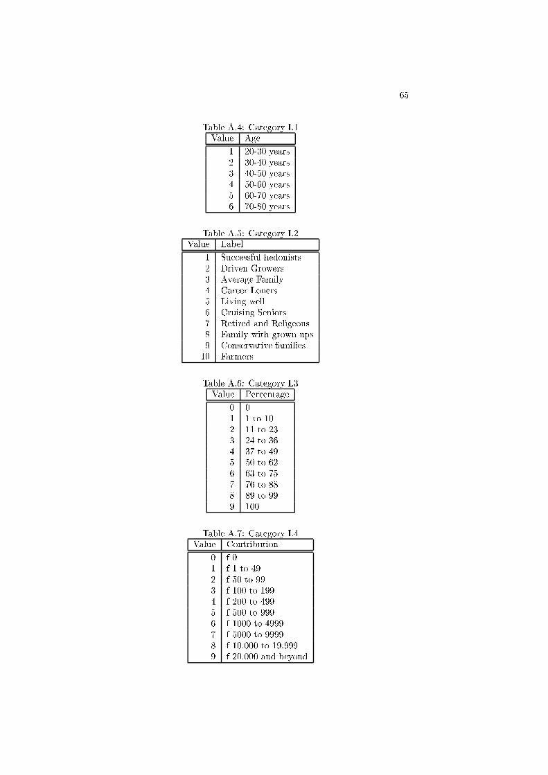
65
Table A.4: Category L1
Value Age
1 20-30 years
2 30-40 years
3 40-50 years
4 50-60 years
5 60-70 years
6 70-80 years
Table A.5: Category L2
Value Label
1 Successful hedonists
2 Driven Growers
3 Average Family
4 Career Loners
5 Living well
6 Cruising Seniors
7 Retired and Religeous
8 Family with grown ups
9 Conservative families
10 Farmers
Table A.6: Category L3
Value Percentage
0 0
1 1 to 10
2 11 to 23
3 24 to 36
4 37 to 49
5 50 to 62
6 63 to 75
7 76 to 88
8 89 to 99
9 100
Table A.7: Category L4
Value Contribution
0 f 0
1 f 1 to 49
2 f 50 to 99
3 f 100 to 199
4 f 200 to 499
5 f 500 to 999
6 f 1000 to 4999
7 f 5000 to 9999
8 f 10.000 to 19.999
9 f 20.000 and beyond

66 APPENDIX A. TABLES OF THE FEATURES AND DATASETS

Bibliography
[1] K.A. Forcht and K. Cochran, "Using Data mining and Dataware-housing
techniques", Industrial Management and Data Systems, 1999
[2] J.R. Bult, Target selection for direct marketing,PhD thesis, Rijks Univer-
siteit Groningen, The Netherlands, 1993
[3] J. Donovan, D.I.Y. direct marketing, Kogan Page Ltd. London, 2000
[4] V.G. Morwitz and D.C. Schmittlein, "Testing new direct marketing of-
ferings: The interplay of management judgment and statistical models",
Management Science vol. 44, No. 5, pp. 610-628, May 1998
[5] R. Webber, "Intelligent systems for market segmentation and local market
planning", Intelligent systems for �nance and business, John Wiley and
Sons Ltd England, 1995.
[6] W.H. Greene, Econometric Analysis, Macmillan Publishing Company New
York, 1993
[7] M. Setnes and U. Kaymak, "Fuzzy modeling of client preference from large
data sets: an application to target selection in direct marketing", IEEE
Transactions on Fuzzy Systems, vol. 9, No. 1, 2001
[8] G.V. Kass, "An exploratoty technique for investigating large quantaties of
categorical data Applied Statistics vol. 29, No. 2, pp. 119-127, 1980
[9] M. Ben-Akiva and S.R. Lerman, Discrete choice analysis: Theory and Ap-
plication to Travel Demand, MIT Press England, 1985
[10] U. Fayyad, G. Piatetsky-Shapiro and P. Smyth, "Knowledge discovery and
Data mining: towards an unifying framework", Proceedings of KDD-96:
International Conference on Knowledge Discovery and Data mining, pp.
82-88, 1996
[11] J. Kleinberg, C. Papadimitriou and P. Raghavan, "A microeconomic view
of data mining", Data mining and knowledge discovery 2, pp 311-324, 1998
[12] R. Babuska, Introduction to Neural Networks, Delft University of Technol-
ogy, 2000
[13] L. Breiman, J.H. Friedman, R.A. Olshen and C.J. Stone, Classi�cation and
Regression Trees, Wadsworth: Belmont USA, 1984
67

68 BIBLIOGRAPHY
[14] D.M. Hawkins and G.V. Kass, "Automatic Interaction Detection", Top-
ics in Applied Multivariate Analysis, pp. 267-302, Cambridge Univ Press:
Cambridge, 1982
[15] E.B. Moser, "Chaid-like Classi�cation Trees", Multivariate Statistics,
course material, www.stat.lsu.edu.faculty/moser/exst7037/exst7037.html,
2000
[16] J. Magidson, "Improved statistical techniques for response modeling-
Progression beyond regression", Journal of Direct Marketing vol. 2 No.
4 pp 6-18, 1988
[17] J. N. Morgan and J. A. Sonquist, "Problems in the analysis of survey data,
and a proposal", Journal of the American Statistical Association, vol. 58
pp. 415-434, 1963
[18] J. A. Sonquist, E. L. Baker and J. N. Morgan, Searching for Structure,
Institute for Social Research, University of Michigan, Ann Arbor, 1973
[19] D. Shepard, The New Direct Marketing, 2nd edition, Irwin Professional
Marketing, 1995
[20] S. J. Long, Regression Models for Categorical and Limited Dependent Vari-
ables, Sage Publications, 1997.
[21] J. Zahavi and N. Levin, "Applying neural computing to target marketing",
Journal of Direct Marketing, vol. 11 No. 4 pp. 77-93, 1997
[22] D. J. Finney, Probit Analysis, Cambridge University Press, UK, 1964
[23] N. Draper and H. Smith, Applied regression analysis, New York: John
Wiley & Sons, 1966 (Revised ed., 1981)
[24] J. R. Quinlan, C4.5: Programs for Machine Learning, Ca, USA: Morgan
Kaufmann Publishing, 1993
[25] D. G. Morrison, "On the Interpretation of Discriminant Analysis", Journal
of Marketing Research, pp. 156-163, 1969
[26] N. Levin and J. Zahavi, Predictive modeling us-
ing segmentation, http://www.urbanscience.com/ Predic-
tive Modeling Using Segmentation.pdf, 1999
[27] R. Lowry,Concepts and Applications of Inferential Statistics, interactive
statistics textbook, http://faculty.vassar.edu/ lowry/ch8pt3.html, 1999
[28] Y. Freund and R. E. Schapire, "Experiments with a new boosting algo-
rithm", Proceedings International Conference on Machine Learning, pp
148-156, Morgan Kaufmann, San Francisco, 1996
[29] Garson, Logistic regression, lecture notes,
http://www2.chass.ncsu.edu/garson/pa765/logistic.htm, 2000
[30] S. Quigley, "Regression analysis", SST Help guide
http://emlab.berkely.edu/sst/regression.html

BIBLIOGRAPHY 69
[31] R. Potharst, U. Kaymak and W. Pijls, "Neural networks for target selec-
tion in direct marketing", Neural networks in Business: techniques and
application, pp 89-110, Idea Group Publishing, London, 2002
[32] SPSS Inc., SPSS Chaid for Windows 6.0, Prentice -Hall, 1993