Urmas Sepp

Factors of Trade-Deficit Convergencein Estonia

Working Papers of Eesti Pank No 1,1999

Urmas Sepp

Factors of Trade-Deficit Convergencein Estonia

Analysis Based on Propensity to Import

Working Papers of Eesti Pank No 1, 1999

Tallinn

RAHVUSRAAMATUKOGU

For information about subscription, call (372) 6 310 920 or (372) 6 310 917; Fax (372) 6 310 954; e-mail: info@epbe.ee

Executive Editor: Ants Kaasik

ISBN 9985-9204-7-3

Printed in the Tallinna Raamatutrükikoda

The author, URMAS SEPP, was born in Tallinn on April 29, 1956.

He graduated from Tallinn Polytechnic Institute cum laude in 1978. In 1984 he became Candidate of Sciences in Economics (Dissertation: The Time Factor of Investment Process and the Economic Efficiency of Production (based on the example of Estonia)). In 1989 he was awarded PhD in Economics (Dissertation: Concept of Synthetic Components of Production Growth).

He has worked as Research Worker and Department Head at the Institute of Economics of the Estonian Academy of Sciences, as Professor at Tallinn Polytechnic Institute and as Economic Adviser at Hansapank. He has been a Member of Government Council, Economic Reform Committee, Future Congress of Estonia, and Price Commission. He has also been an Expert of the International Group for Macroanalysis of Estonian Economy, and of the Group of the CPI. From 1993 he has been working at Eesti Pank (Bank of Estonia). He has been Deputy Head of the Central Bank Policy Department and is Head of Macroeconomic Research Department at present. He is also a Member of Doctoral Degree Council of Tallinn Technical University and of the Scientific Council of the Institute of Economics of Tallinn Technical University.

U. Sepp has written over 160 scientific publications.

He is married and has two daughters.

CONTENTS

0. Introduction 51. Problem 62. Modelling of Imports 73. Import Factors 74. Import Propensity 95. Estimation of Import Propensity: a Concept 106. Equations of the System 11

6.1. Imported Input of Export Production 116.2. Import Propensity of External Demand 116.3. Import Propensity of Domestic Demand 11

7. Data 128. Solution of System 129. Empirical Equations 13

9.1. Import Propensity of Domestic Demand 139.2. Price Level as a Factor of Import Propensity 149.3. Import Propensity of Foreign Demand 15

10. Levels of Import Propensities 1611. Simulation of the Trade Balance 1712. Perspectives for Trade Balance Convergence 1813. Conclusions 2214. References 23

The author is grateful to Rasmus Pikkani and Mari Rell for their assistance in empirical work.

0. Introduction

The present paper is a sequel of Export-Led Growth with Its Trade-Balance Effect in Estonia (the paper for the 45th International Atlantic Economic Conference, session “Economics of Transition to Market Economies”, Rome, March 16-21, 1998) and Export Growth and Trade Balance in Estonia (the paper for the 4th Conference on Financial Sector Reform in Central and Eastern Europe, Tallinn, April 24-26, 1998; published in Working papers in Economics. Tallinn Technical University, No 98/20).

Estonian export statistics has substantially changed since the time the research underlying the above articles was finalised. Due to more accurate data on trade becoming available, the balances of payments for 1996 and 1997 have been adjusted. Firstly, the State Statistical Office and the Customs Board adjusted the foreign trade figures for 1997 as a result of which the imports increased by nearly EEK 2 billion and the exports by EEK 700 million. Secondly, the exports also increased due to the revision by Eesti Pank, when the price transformations affecting goods exported through customs warehouses and not reflected in the foreign trade statistics were taken into due account. In 1996, those transformations accounted for more than EEK 300 million and in 1997 approximately EEK 2.1 billion (Eesti Pank 1998).

The adjustments of statistics have important consequences. First of all, adjusted data show that contrary to the earlier statistics, the trade deficit level had not essentially deteriorated.

Naturally, the adjustments in statistics and the changed vision have to be reflected in the main behavioural equations of the Estonian economy. Functions of import demand are most definitely such equations.

To take into account this and other new aspects, I have revised my earlier papers, the outcome of which is the present paper.

The paper is structured in the following way. In the first Section there is presented the problem of trade deficit in the case of export-led economic growth.

The instruments (models, factors and indicators) needed for dealing with the problem are considered in Sections 2... 4. While specifying the import demand function, the indicator of import propensity has been used. Preference to propensity instead of the conventional form of demand equation was pragmatically justified in view of the empirical experience. The advantage of propensity-based model revealed itself in the forecast of the actually witnessed break in the Estonian import trend, which the conventional function of import demand failed to reflect.

The next part of the paper (Sections 5 & 6) gives a brief description of difficulties in empirical use of propensity indicators. The estimation of import propensities of domestic and external demand is impaired by the scarcity of information. Nevertheless, there is a chance to cross the information problem. A way of a solution is introduced in the paper.

Inputs and outcomes of the empirical estimation as well as the estimation process itself are presented in Sections 7...9. Despite the high explanatory power, the estimated equations were not the best in the statistical sense. The prevailing trouble was the distribution of the residuals different from the white noise. The adequacy of the equation has also been studied with the help of forecast performance. According to the division of the Theil coefficient the ex-post dynamic forecast was slightly biased.

Besides, the factors included in the equation of no lesser interest present the set of possible explanatory variables left out from the equation, the price indicators and the real exchange rate in the first place. Contrary to the theoretical and intuitive expectations, the real effective exchange rate or the change of the relative price level did not turn out to be the factors of import propensity in Estonia.

Some speculations about the reasons why real exchange rate or other similar variables happened to be useless in import modelling are presented in Section 9.2.

The last part of the paper (Sections 10... 12) summarises the characteristic features of import propensity and perspectives for the convergence of the trade deficit in a very general way. The principal rationale of the analysis was the convergence of the trade balance. In other words I was interested whether and to what extent the different factors would determine the improvement of the deficit. The central issue of the analysis was the trade balance effect of export as the major determinant of economic growth.

The measurement of impacts was performed on the basis of dynamic elasticities, produced by deterministic simulations, and using the impulse response analysis. The results of simulation are concluded in brief in the last Section of the paper.

1. Problem

In 1996, the negative trade and services balance1 of Estonia crossed, for the first time, as the average for the year, the threshold of 10% GDP. The level of deficit was expressed by a two-digit figure in 1997, too; so was it in 1998, according to a preliminary estimate. The high level of deficit was the outcome of neither the decrease in exports nor its sluggish increasing rate. Quite the opposite - the exports of Estonia have picked up considerably2.

Export being the main driving force in a small open economy, a question suggests itself of whether the economic growth in Estonia will be accompanied by a rapid growth of imports and the worsening of trade balance (or a consistently high level of its deficit). The goal of the paper is to cast light on whether it is endemic for the exports in Estonia to have the negative effect on trade balance. The question is whether the deficit dynamics is a diverging or a converging process under the conditions of export-led economic growth.

A good example for illustration of the problem is the Lamfalussy type model. In the Lamfalussy model3 the negative impact of growth in exports is accounted for high marginal propensities to import and to invest (depending on the exports) with low marginal propensity to save. When interpreting deficit, it may come in question whether the marginal propensities exceed critical values for producing convergence. In the case of affirmative answer, the system will not bring itself into equilibrium without intervention4.

In case of a converging process, the propensities are below the critical values and there is a hope for the breakdown in the growth trend of deficit and its decline to the level of a (long-term) equilibrium.

1 Hereinafter some abbreviated terms will be used. If unspecified, export will mean trade and services export, import will mean trade and services import, trade balance/deficit will mean the net export of goods and services.

2 Nominal growth of exports of goods in 1997/6 amounted to 42.85%.

3 Traditional reference Lamfalussy (1963).

4 The problem is presented as well in framework of more advanced models. For example, Osang- Pereira (1997) shows that in a small economy the domestic attitude towards saving, as indicated by the intertemporal elasticity of substitution, plays a crucial role. If domestic consumers are preferring consumption to saving, foreign growth may lead to lower domestic output growth than otherwise. So, the foreign growth is not a substitute for a weak domestic attitude toward saving.

2. Modelling of Imports

It is necessary to build an adequate model in order to find out the possible convergence or divergence of the trade balance. The balance of imports and exports is not a problem, involving only those two phenomena. According to Bruce and Purvis the trade balance must satisfy certain accounting identities:

T = NX = Y- A = H - I,

T is trade balance, NX - net exports, Y - output, A - absorption, H - savings, I - investments.

The identities illustrate that there are three equivalent measures of the external balance, and each has been the point of argument in the theory of external balance. The real model focuses on NX and explains it in terms of the factors underlying the level of expenditure on distinct export and import goods. The monetary model focuses on the differences between aggregate levels of output and expenditure as given by Y - A. The third model assumes that T is based on factors underlying the saving and/or investment decisions. (Bruce-Purvis, 1984, p 844).

Due to the complexity, the answer for the problem of trade balance is to be sought with the help of a model describing the whole economy. Conventional instruments for the solution of the trade problems are the computable general equilibrium models (Dervis-de Melo-Robinson, 1982) and expectations- based equilibrium models (Gandolfo-Padoan, 1990). The calibration of macromodels calls for precise information regarding not only the macrolevel of the national economy, but also the institutional sectors and markets. Unfortunately, the information required for the application of general equilibrium models is not available for Estonia.

Compounding the situation is the lack of information needed for the construction of an econometric macromodel, including the crucial adaptation mechanisms of the Estonian economy. On one hand, the scarcity of information is due to the lack of fundamental economic indicators. On the other hand, it is related to the shortness of history of sovereign Estonia (and its economy). The development of transition economies being overly dynamic, the relations between economic variables are unstable, as a general rule. Therefore the estimation of an adequate macromodel calls for many more observations than provided by the short period of independence.

3. Import Factors

The imperfect and the perfect substitute models have dominated as general models of trade in the empirical literature. In case of both models the explanatory variables of import demand are income and price(s)5;6.

The imperfect substitute model allows for the deviation from the law of one price. This is quite typical for the post-socialist transition economies including Estonia, undergoing the (price) convergence process, (cf Sepp, 1996). According to the import demand equation of the imperfect substitute model is:

M - f (Y, PI, P), fl, D > 0, f2<0

5 This specification is supported by the micro- and macroeconomic derivations of import demand function (Senhadji, 1997; Senhadji-Montenegro, 1998).

6 Overview of empirical research, where import is specified as the function of income and prices is presented in Goldstein-Khan, 1984; (earlier works) and by Senhadji-Montenegro, 1998; (recent works).

Y- income, PI and P- the prices of imports and domestically produced goods.

It is assumed that in accordance with the conventional theory, the consumer is postulated to maximise the utility subject to a budget constraint. The resulting demand function for imports represents the quantity demanded as a function of the level of (money) income in the importing region, the price of the imported goods, and the price of domestic substitutes. For aggregate imports, the possibilities of inferior quality and the domestic complements for imports are typically excluded, so that income and cross-price elasticities are assumed to be positive, whereas the own-price elasticity of demand is expected to be negative (Goldstein-Khan, 1984, p 1046)7.

In its most common form, the homogeneity of the demand function is expressed by dividing the right hand side of the equation by P, so that the two arguments of the demand function will become the real income (Y/P) and the relative price of imports (PI/P). (Goldstein-Khan, 1984, p 1046).

In empirical treatments the explaining variables of the import equation are often presented as transformed. For example, instead of separate price variables the real exchange rate is often used8.

Secondly, income is frequently proxied with the variables representing the domestic demand9. This approximation has a principal background for modelling the Estonian economy. Using demand as an import determinant suits the currency board regime reigning in Estonia. Under the market driven currency board the non-discretionary monetary policy means that the money supply could be settled not only by the demand but also by the surge of capital inflow. The last argument makes the currency board in principle similar to the economy using the gold standard and the effects of capital inflow in case of the currency board analogous to the model of gold standard10.

7 In empirical forms of the import equations are naive to compare with concepts of the conventional economic theory. Goldstein and Khan give as examples the neglect of “permanent” or “life-cycle” income constructs in import and export demand functions and the absence of “expected” prices from export and supply functions. Given the maintained hypothesis that imports and exports are (imperfect) substitutes for domestic goods, it does not make sense to have one theory of consumption or of aggregate supply for domestically produced goods and another, quite different for imports and exports (Goldstein-Khan, 1984, p 1098).

8 Khan, M.S.- Knight, M.D. (1991); Vaez-Zadeh.,R. (1991); Aghevli, B.B.-Sassanpour, C. (1991).

9 Fisher-Whitley (1998); Laxton (1998); Lipschitz (1991).

10 The effects of capital inflow in an small open economy operating under a gold standard when

A) the prices remain constant (ie PPP holds):

The gold inflow will translate into an increase in the domestic money supply. A small open economy will have to face the international prices for all goods produced and consumed. Under the gold standard, the fixed international value of its own currency will fix the domestic prices of all goods. The gold inflow will exert no influence on domestic prices, but the increase in the domestic money will increase the general level of demand in the economy. At the given domestic price, the volume of import demand will rise.

B) the prices are changing:

The small open economy assumption will be maintained in terms of the domestic economy’s inability to influence foreign prices of non-traded goods, but consideration will be given to a class of domestic goods traded on international markets. Again, the capital inflow will give rise to an increase in imports and decrease in exports, but it will do so, partly by pushing up prices of non-tradable relative to tradable goods, which will shift the production away from tradable and the consumption towards tradable. (Bruce-Purvis, 1984, p 837-8).

Thirdly, the import equation has also been extended by inclusion of the external demand (Alexius, 1993)". This modification is in line with the particularities of Estonia where the export consists 77% of GDP in 1997. Export is the source of income making it an influential factor of import. On the other hand, exports present a large proportion of the aggregate demand. As export production needs imported inputs, the export is due to the technological reasons an important factor of the import demand.

4. Import Propensity

While specifying the import demand function, the indicator of import propensity was used. Preference to import propensity instead of the conventional form of import demand equation was pragmatically justified in view of the empirical experience. The advantage of propensity-based model exposed itself in the forecast of the actually witnessed break in the Estonian import trend, which the conventional function of import demand failed to reflect. The cause for adequacy of import propensity lies in the sensitivity of the propensity indicator to the behavioural deviations, which are typical for the Estonian economy. The behavioural changes result from the underlying quality of the Estonian economy, ie from the vibrant transition process. On the other hand, the variation of import propensity stems from the core of the currency board system, where the excessive money supply resulting from capital surge is “sterilised” by financing the imports.

The import propensity is regularly expressed with respect to income. However, that is by far not the sole option. For example, Laursen and Metzler (1959) in their dynamic model of exchange rate and income scaled the import propensity using the domestic demand11 12.

The propensity characterising demand is preferred also in analysing the developments in the Estonian trade deficit. The use of demand as the scale for the propensity was conditioned by the basic nature of the Estonian economy. One has to admit again that the Estonian economy operates according to the rules of the currency board. As mentioned above, it means that a good part of capital inflow is sterilised via import. So, in the case of variation of capital inflow the import propensity, expressed in respect of demand (what is to some extent financed by external capital), tends to be more stable comparing with the indicator of income-based propensity.

The components of final demand have different import contents. The investments in Estonia as a small economy are relatively import-intensive. The share of investments in generating imports is crucial because Estonia, as a typical under-capitalised post-socialist economy is characterised by an urgent need for capitalisation. Keeping in mind the rise in investments, on one hand, and the higher imports coherence of the investments, on the other hand, a rise in imports and import propensity could be presumed.

Yet, the development of other components of consumption does not need to decrease the imports. According to the consumer survey by Saar Poll, the import preference regarding foodstuffs was 20- 24%. Regarding durable and consumer goods the same index amounted to 90% (Traks-Männik, 1997). Together with the growth of income and wealth, the decrease in food demand and the increase of demand for lower priority goods in private consumption was evident. So, due to import preference the growth of income and wealth causes a change of the demand structure accompanied by an increase of import propensity13.

11 To point out the role of export Kohler (1996) presented import as the function of export solely.

12 Domestic demand will hereinafter mean the domestic absorption or the aggregate demand for goods by residents, while ignoring the residency of suppliers.

13 Arestis-Howells (1995) underline that higher income earners have higher import propensities.

To allow for different propensities, separate import propensities for each category of absorption and for exports have to be calculated using data from input-output matrices14. Regrettably the last input- output table in Estonia was compiled in the middle of the last decade and is now completely outdated. The maximum that one can do is to consider two components of aggregated demand (AD) - the domestic demand (DD) and foreign demand (X), which have probably different import contents and propensities.

Since AD = DD + X, the import propensity of aggregate demand AD ik = M/AD depends on the import propensities of domestic demand (DD ik) and of foreign demand (X ik):

DD ik = Md/DD,Md is the import for the domestic final consumption and for the production giving output for

the domestic market. DD ik shows the fraction of import in satisfying the domestic demand.

X_ik=Mx/X,

Mx is the import for the production giving output for the external market. X_ik shows ratio of the import needed to meet the foreign demand.

According to the definition, the import propensity of aggregate demand is the average weighted by the share of components of AD ik = w * DD ik + (1-w) * X ik,

w = DD/AD

5. Estimation of Import Propensity: a Concept

The estimation of import propensities of domestic and external demand is impaired by the scarcity of information, ie the distribution of import as per Mx and Md is unknown. Nevertheless, there is a chance to cross the information problem.

There is relatively more information about the imported inputs of export production. The customs statistics provides Mxt, the import brought in Estonia for manufacturing under international subcontracting. The imported input of the rest of export, Mxv, is still unknown: Mx = Mxt + Mxv.

Regarding the import to meet the domestic demand, the official statistics fails to provide information. However, the wanted variable can be found by elimination, ie by subtraction from the total the import for export production: Md = M - Mxt - Mxv

Consequently, to estimate the import propensities of domestic and foreign demand, Mxv is to be found. The problem of finding of Mxv can be solved simultaneously with the estimation of import propensity equations. Hence, we arrange the system of equations:(1) AD ik = w * (M- Mx(Z 1 ))/DD + (1-w) * Mx(Z 1 )/X ,(2) (X_ik =) Mx/X = X(Z2),(3) (DD ik =) Md/DD = DD{Z3),

Z1 - factors of import input of export production, Z2- factors of import propensity of foreign demand, Z3 - factors of import propensity of domestic demand.

14 See Laxton, 1998, p 57.

6. Equations of the System

6.1. Imported Input of Export Production

Due to the absence of the theoretical suggestions, the equation for imported inputs of export production has been specified at our own discretion. By definition, Mx = Mxt + Mxv, where Mx is known. So Mxv is presented as the first approximation to be dependent on the Mxt, ie Zl=Mxv.

It was also assumed that M(Z1) is a linear function excluding constant15 and the ratio of Mxv to Mxt is changing according to the share of international subcontracting in export production, S16

Mx(Zl) = Mxt + Mxv(Mxt, S) + el ie

(la) Mx(Zl) = Mxt * (1 + X.+ P*S) + el, where X and 0 are parameters.

6.2. Import Propensity of External Demand

The import propensity of external demand is rather stable in short-run, for export production conditions and the composition of inputs do not change, to any significant degree, in the short-term perspective. We proceeded from the fact that the subcontracting has a higher import content, and that the increase in subcontracting means a greater import content of exports17. So, the import propensity of external demand changes, in the short term, only in case the share of re-export of goods imported for processing (for subcontracting) increases or decreases in export.

Hence Z2 = S and the equation:Mx/X = X(S) + 62 or taking into consideration the equation (la)

(1 + X+ P*S)* Mxt)/X = X(S) + 62, wherefrom

(2a) Mxt/X = X(S)/( 1 + X+ P*S) + e2

6.3. Import Propensity of Domestic Demand

According to the models of Section 3 the import demand (and the propensity to import as well18) depends on the income, on domestic and foreign prices19, and on the export. Due to the different

15 All equations of the system (l)-(3) were expected to be linear. The linearity hypothesis has been examined with the RESET-test.

16 It was expected that in the case of a significant share of subcontracting in export production, the relative amount of imported inputs of export production is higher than otherwise.

17 For example, the change of import propensity of aggregate demand in 1996-1997 (propensity being 44% and 45.8%, respectively) can be explained, among other factors, by the 60% increase (compared to the previous year) of re-export of goods imported for processing.

18 It was assumed that the factors of import propensity are the same as of the import demand.

19 KEER, CPI, the inflation index of non-tradable goods, NT, the inflation index of tradable goods, T, as well as NT/T were used.

import content of components of absorption (see Section 4), the import propensity depends on the structure of demand. To reflect the structural shifts the shares of consumption and investments in the GDP were used.

Under the currency board regime the capital flows initiate the adaptation mechanism that includes also imports (see Section 3). Furthermore, the import propensity is directly affected by the capital inflow. Financial resources attracted from abroad are first and foremost used for financing the investments and for purchasing durable goods (eg cars, home appliances). As a rule, the import content of investments and durable goods is higher than that of other categories of demand.

The external capital reaches the domestic demand primarily through financial intermediation. Therefore the inflow of capital is proxied in the propensity equation by indicators of financial intermediation (such as the flow and stock of credits extended to households and to corporate sector and the interest rates).

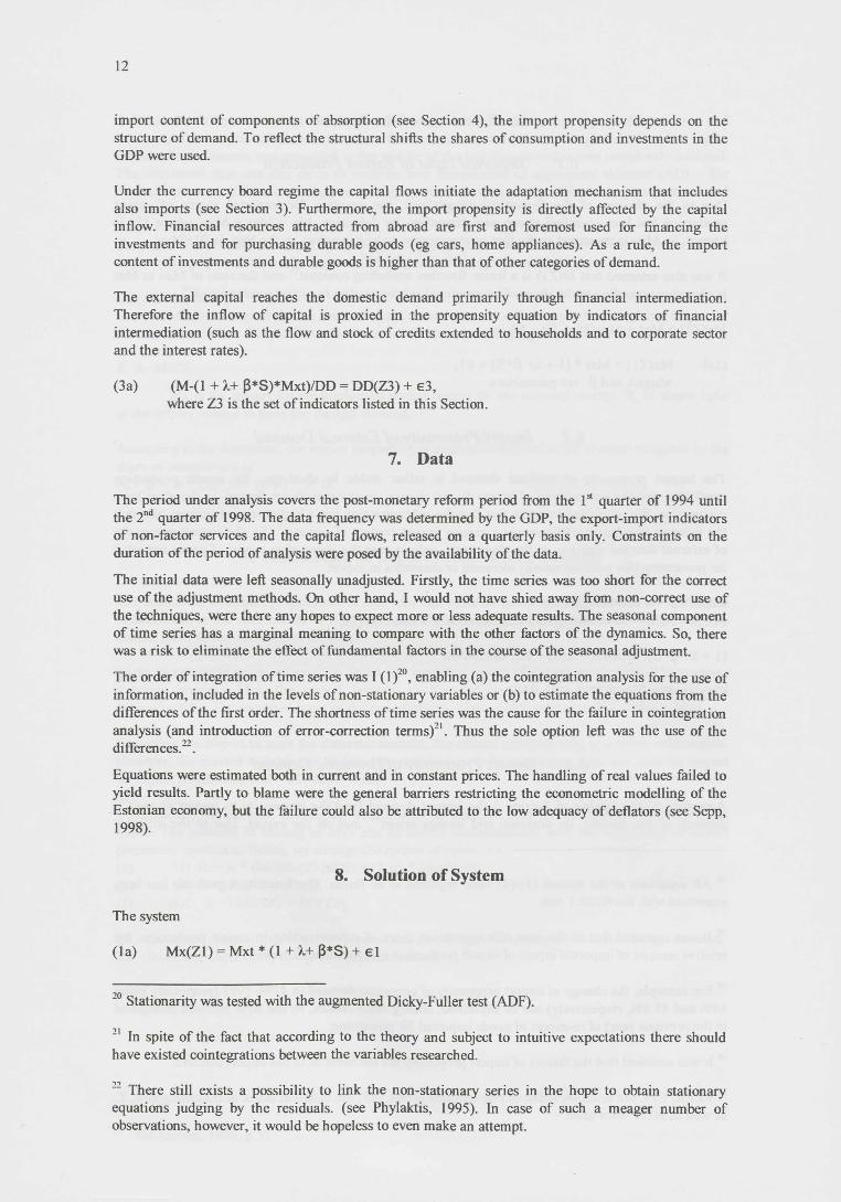
(3a) (M-(l + 1+ P*S)*Mxt)/DD - DD(Z3) + e3,where Z3 is the set of indicators listed in this Section.

7. Data

The period under analysis covers the post-monetary reform period from the 1st quarter of 1994 until the 2nd quarter of 1998. The data frequency was determined by the GDP, the export-import indicators of non-factor services and the capital flows, released on a quarterly basis only. Constraints on the duration of the period of analysis were posed by the availability of the data.

The initial data were left seasonally unadjusted. Firstly, the time series was too short for the correct use of the adjustment methods. On other hand, I would not have shied away from non-correct use of the techniques, were there any hopes to expect more or less adequate results. The seasonal component of time series has a marginal meaning to compare with the other factors of the dynamics. So, there was a risk to eliminate the effect of fundamental factors in the course of the seasonal adjustment.

The order of integration of time series was I (l)20, enabling (a) the cointegration analysis for the use of information, included in the levels of non-stationary variables or (b) to estimate the equations from the differences of the first order. The shortness of time series was the cause for the failure in cointegration analysis (and introduction of error-correction terms)21. Thus the sole option left was the use of the differences.22.

Equations were estimated both in current and in constant prices. The handling of real values failed to yield results. Partly to blame were the general barriers restricting the econometric modelling of the Estonian economy, but the failure could also be attributed to the low adequacy of deflators (see Sepp, 1998).

8. Solution of System

The system

(la) Mx(Zl) = Mxt * (1 + 1+ £*S) + €l

20 Stationarity was tested with the augmented Dicky-Fuller test (ADF).

21 In spite of the fact that according to the theory and subject to intuitive expectations there should have existed cointegrations between the variables researched.

22 There still exists a possibility to link the non-stationary series in the hope to obtain stationary equations judging by the residuals, (see Phylaktis, 1995). In case of such a meager number of observations, however, it would be hopeless to even make an attempt.

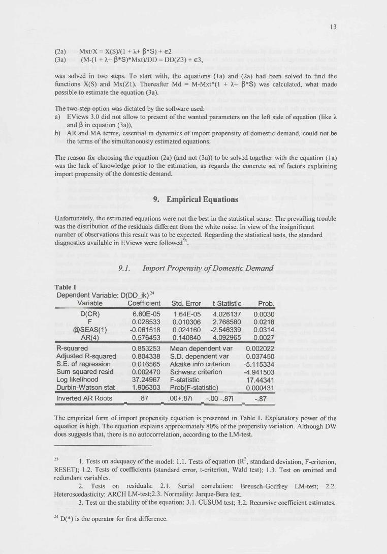
(2a) Mxt/X = X(S)/( 1 + 1+ |3*S) + 62(3a) (M-(l + 1+ |3*S)*Mxt)/DD = DD(Z3) + €3,

was solved in two steps. To start with, the equations (la) and (2a) had been solved to find the functions X(S) and Mx(Zl). Thereafter Md = M-Mxt*(l + X.+ |3*S) was calculated, what made possible to estimate the equation (3a).

The two-step option was dictated by the software used:a) EViews 3.0 did not allow to present of the wanted parameters on the left side of equation (like 1

and P in equation (3a)),b) AR and MA terms, essential in dynamics of import propensity of domestic demand, could not be

the terms of the simultaneously estimated equations.

The reason for choosing the equation (2a) (and not (3a)) to be solved together with the equation (la) was the lack of knowledge prior to the estimation, as regards the concrete set of factors explaining import propensity of the domestic demand.

9. Empirical Equations

Unfortunately, the estimated equations were not the best in the statistical sense. The prevailing trouble was the distribution of the residuals different from the white noise. In view of the insignificant number of observations this result was to be expected. Regarding the statistical tests, the standard diagnostics available in EViews were followed23.

9.1. Import Propensity of Domestic Demand

Table 1Dependent Variable: D(DD_ik)24

Variable Coefficient Std. Error t-Statistic Prob.D(CR) 6.60E-05 1.64E-05 4.026137 0.0030

F 0.028533 0.010306 2.768580 0.0218@SEAS(1) -0.061518 0.024160 -2.546339 0.0314

AR(4) 0.576453 0.140840 4.092965 0.0027R-squared 0.853253 Mean dependent var 0.002022Adjusted R-squared 0.804338 S.D. dependent var 0.037450S.E. of regression 0.016565 Akaike info criterion -5.115334Sum squared resid 0.002470 Schwarz criterion -4.941503Log likelihood 37.24967 F-statistic 17.44341Durbin-Watson stat 1.906303 Prob(F-statistic) 0.000431Inverted AR Roots .87 .00+.87i -.00 -,87i -.87

The empirical form of import propensity equation is presented in Table 1. Explanatory power of the equation is high. The equation explains approximately 80% of the propensity variation. Although DW does suggests that, there is no autocorrelation, according to the LM-test.

1. Tests on adequacy of the model: 1.1. Tests of equation (R1 2 3, standard deviation, F-criterion, RESET); 1.2. Tests of coefficients (standard error, t-criterion, Wald test); 1.3. Test on omitted and redundant variables.

2. Tests on residuals: 2.1. Serial correlation: Breusch-Godfrey LM-test; 2.2. Heteroscedasticity: ARCH LM-test;2.3. Normality: Jarque-Bera test.

3. Test on the stability of the equation: 3.1. CUSUM test; 3.2. Recursive coefficient estimates.

24 D(*) is the operator for first difference.

It was only CR, the stock of credits extended to households, that could be included into the equation as the sole meaningful explanatory variable. In view of the role of capital flows in generating imports under the currency board regime the result was only to be expected. The other terms of the equation are components of the time-series model. AR(4) shows the proportional dependence on the values of the same quarter of the past year, indicative of the inertia in the tendency as well in the seasonality of import propensity. The parameter of AR(4) suggests the converging process. Seasonality in the change of propensity is expressed also with a special variable @SEAS(1) which reflects lower import propensity in the first quarter of the year that is in accordance with the regularity of import dynamics. F is a dummy marking the particularities of the second half of 1995.

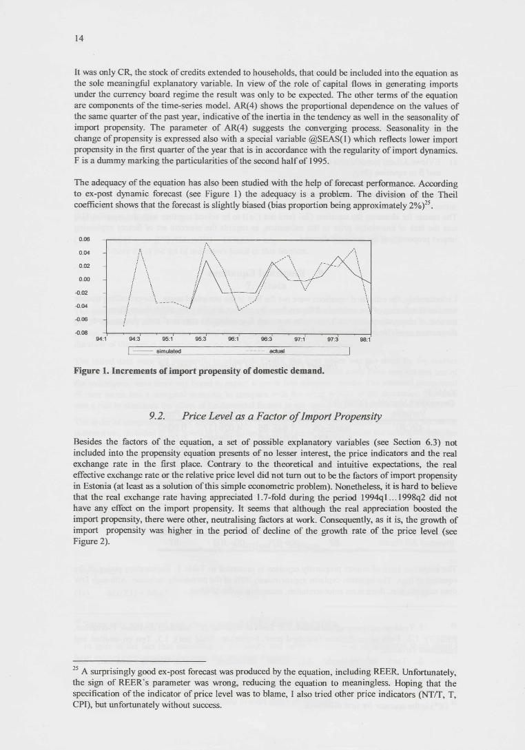
The adequacy of the equation has also been studied with the help of forecast performance. According to ex-post dynamic forecast (see Figure 1) the adequacy is a problem. The division of the Theil coefficient shows that the forecast is slightly biased (bias proportion being approximately 2%)25.

-0.04

-0.06

simulated

Figure 1. Increments of import propensity of domestic demand.

9.2. Price Level as a Factor of Import Propensity

Besides the factors of the equation, a set of possible explanatory variables (see Section 6.3) not included into the propensity equation presents of no lesser interest, the price indicators and the real exchange rate in the first place. Contrary to the theoretical and intuitive expectations, the real effective exchange rate or the relative price level did not turn out to be the factors of import propensity in Estonia (at least as a solution of this simple econometric problem). Nonetheless, it is hard to believe that the real exchange rate having appreciated 1.7-fold during the period 1994ql... 1998q2 did not have any effect on the import propensity. It seems that although the real appreciation boosted the import propensity, there were other, neutralising factors at work. Consequently, as it is, the growth of import propensity was higher in the period of decline of the growth rate of the price level (see Figure 2).

25 A surprisingly good ex-post forecast was produced by the equation, including REER. Unfortunately, the sign of REER’s parameter was wrong, reducing the equation to meaningless. Hoping that the specification of the indicator of price level was to blame, I also tried other price indicators (NT/T, T, CPI), but unfortunately without success.

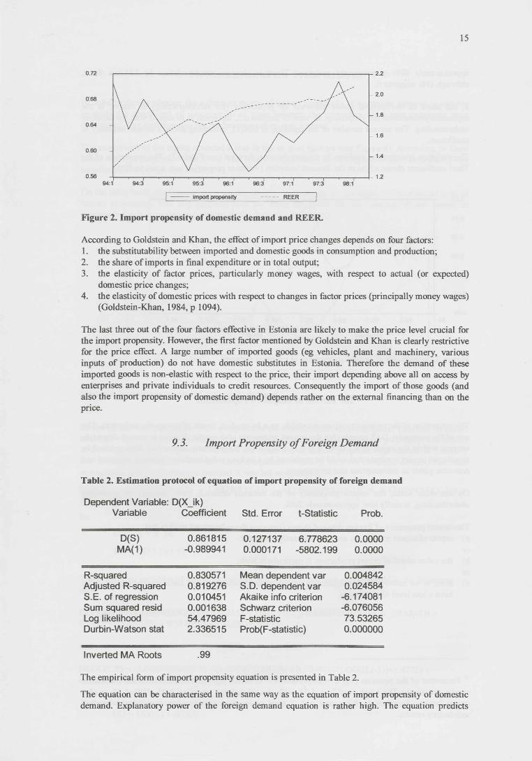
import propensity REER

Figure 2. Import propensity of domestic demand and REER.

According to Goldstein and Khan, the effect of import price changes depends on four factors:1. the substitutability between imported and domestic goods in consumption and production;2. the share of imports in final expenditure or in total output;3. the elasticity of factor prices, particularly money wages, with respect to actual (or expected)

domestic price changes;4. the elasticity of domestic prices with respect to changes in factor prices (principally money wages)

(Goldstein-Khan, 1984, p 1094).

The last three out of the four factors effective in Estonia are likely to make the price level crucial for the import propensity. However, the first factor mentioned by Goldstein and Khan is clearly restrictive for the price effect. A large number of imported goods (eg vehicles, plant and machinery, various inputs of production) do not have domestic substitutes in Estonia. Therefore the demand of these imported goods is non-elastic with respect to the price, their import depending above all on access by enterprises and private individuals to credit resources. Consequently the import of those goods (and also the import propensity of domestic demand) depends rather on the external financing than on the price.

9.3. Import Propensity of Foreign Demand

Table 2. Estimation protocol of equation of import propensity of foreign demand

Dependent Variable: D(X_ik)Variable Coefficient Std. Error t-Statistic Prob.

D(S)MA(1)

0.861815-0.989941

0.127137 6.7786230.000171 -5802.199

0.00000.0000

R-squared 0.830571 Mean dependent var 0.004842Adjusted R-squared 0.819276 S.D. dependent var 0.024584S.E. of regression 0.010451 Akaike info criterion -6.174081Sum squared resid 0.001638 Schwarz criterion -6.076056Log likelihood 54.47969 F-statistic 73.53265Durbin-Watson stat 2.336515 Prob(F-statistic) 0.000000

Inverted MA Roots .99

The empirical form of import propensity equation is presented in Table 2.

The equation can be characterised in the same way as the equation of import propensity of domestic demand. Explanatory power of the foreign demand equation is rather high. The equation predicts

approximately 80% of propensity variation. There is also no autocorrelation by LM-test there, although DW suggests it.

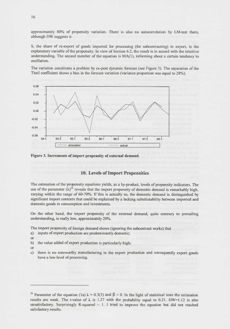
S, the share of re-export of goods imported for processing (for subcontracting) in export, is the explanatory variable of the propensity. In view of Section 6.2, the result is in accord with the intuitive understanding. The second member of the equation is MA(1), informing about a certain tendency to oscillation.

The variation constitutes a problem by ex-post dynamic forecast (see Figure 3). The separation of the Theil coefficient shows a bias in the forecast variation (variance proportion was equal to 28%).

-0.06

simulated actual

Figure 3. Increments of import propensity of external demand.

10. Levels of Import Propensities

The estimation of the propensity equations yields, as a by-product, levels of propensity indicators. The use of the parameter (l)26 reveals that the import propensity of domestic demand is remarkably high, varying within the range of 60-70%. If this is actually so, the domestic demand is distinguished by significant import contents that could be explained by a lacking substitutability between imported and domestic goods in consumption and investments.

On the other hand, the import propensity of the external demand, quite contrary to prevailing understanding, is really low, approximately 20%.

The import propensity of foreign demand shows (ignoring the subcontract works) thata) inputs of export production are predominantly domestic; orb) the value added of export production is particularly high; orc) there is no noteworthy manufacturing in the export production and consequently export goods

have a low level of processing.

26 Parameter of the equation (la) 1 = 0.3(3) and |3 = 0. In the light of statistical tests the estimation results are weak. The t-value of X is 1.27 with the probability equal to 0.21. DW=1.12 is also unsatisfactory. Surprisingly R-squared = 1. I tried to improve the equation but did not reached satisfactory results.

11. Simulation of the Trade Balance

In order to decide whether the estimated model of import propensity of aggregate demand is suitable to study the conditions of convergence of trade balance, the properties of ex-post prognosis were considered. The criterion was the performance of ex-post forecast.

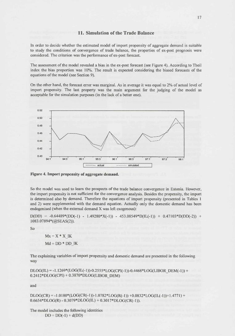
The assessment of the model revealed a bias in the ex-post forecast (see Figure 4). According to Theil index the bias proportion was 10%. The result is expected considering the biased forecasts of the equations of the model (see Section 9).

On the other hand, the forecast error was marginal. As in average it was equal to 2% of actual level of import propensity. The last property was the main argument for the judging of the model as acceptable for the simulation purposes (in the lack of a better one).

actual simulated

Figure 4. Import propensity of aggregate demand.

So the model was used to learn the prospects of the trade balance convergence in Estonia. However, the import propensity is not sufficient for the convergence analysis. Besides the propensity, the import is determined also by demand. Therefore the equations of import propensity (presented in Tables 1 and 2) were supplemented with the demand equation. Actually only the domestic demand has been endogenised (when the external demand X was left exogenous):

D(DD) = -0.64489*(DD(-1) - 1.49280*X(-1)) - 453.08549*D(IL(-1)) + 0.47103 *D(DD(-2)) + 1083.07894*(@SEAS(2)).

So

Mx = X * X IK

Md = DD * DD IK

The explaining variables of import propensity and domestic demand are presented in the following way

DLOG(IL) = -1.1269*(LOG(IL(-1))-0.2555*LOG(CPI(-1))-0.4468*LOG(LIBOR_DEM(-1)) + 0.2412*DLOG(CPI) + 0.3870*DLOG(LIBOR DEM)

and

DLOG(CR) = -1.0180*(LOG(CR(-1))-1.0782*LOG(R(-1)) +0.0832*LOG(IL(-1))+1.4771) + 0.6654*DLOG(R) - 0.3079*DLOG(IL) + 0.3017*DLOG(CR(-l)).

The model includes the following identities DD = DD(-l) + d(DD)

XJK = X IK (-1)+ D(XJK)DD IK = DD IK (-1)+ D(DD JK)M= Mx + Md T = X-M GDP = DD + T TY = T/GDP, where

DD is domestic demand; X is export, M is import; TY is a fraction of trade deficit in GDP; DDik is the import propensity of domestic demand; X_ik is the import propensity of the external demand; Md is the import for the domestic final consumption and for the production giving output for the domestic market; Mx is the import for the production giving output for the external market; IL is the average interest rate of credit; CR is the stock of privat credit; CPI - the consumer price index; LIBOR DEM is the 3-month interest rate of D-marks; R is aggregate credit resource of the commercial banks.

The assessment of impacts was performed on the basis of dynamic elasticities for exogenous variables, produced by deterministic simulations and impulse-response analysis for endogenous variables. The simulations started from 1999ql.

Dynamic elasticities are presented throughout four quarters as of the beginning of the simulation period. The use of four quarters is conditioned by length of the lag (the maximum lag of the equations used in the model is four quarters). If we consider impact elasticity only during the period of exogenous shock, the impact of the factors with lag, which becomes particularly important in equations specified in ECM format, does not show.

12. Perspectives for Trade Balance Convergence

The above-mentioned model was applied in order to assess the following:

a) the impact of different factors on import propensity;

b) the impact of import propensity on trade balance deficit;

c) the role of import propensity (in other words its factors) on the convergence of trade balance deficit with reference to other factors.

The principal rationale of the analysis was the stability of the model and convergence of the trade balance in order to TY~»0. In other words, I was interested whether and to what extent the different factors would determine the improvement of the deficit. The central issue of the analysis was the trade balance effect of export as the major determinant of economic growth.

The dependency of import propensity can be seen in two ways -(a) the direct impact, which is the straight reflection of the factors included in the propensity

equations;(b) the indirect impact, which involves feedback mechanisms, included into the model.

In the case of import propensity of foreign demand (X ik) it is only natural that only the share of re­export (variable S) which is included in the equation participates in the impact (the corresponding elasticity coefficient equals to 0.7%). Since X and S are exogenous, according to the model, the feedback mechanism does not exist for X and X ik and the dependency of import propensity is limited to direct impact (see Figure 3).

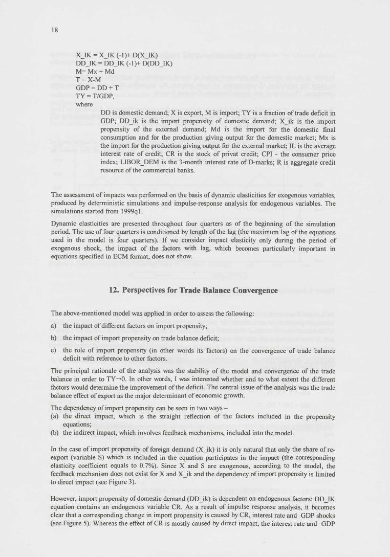
However, import propensity of domestic demand (DD ik) is dependent on endogenous factors: DD IK equation contains an endogenous variable CR. As a result of impulse response analysis, it becomes clear that a corresponding change in import propensity is caused by CR, interest rate and GDP shocks (see Figure 5). Whereas the effect of CR is mostly caused by direct impact, the interest rate and GDP

shocks influence import propensity in a more complex way mainly through increased demand and money supply.

FIGURE 5. DDJK dependency (as the share in SD) on +1 SD shocks of relevant factors

GDP IL

6 72 3

CR M2

DD_ik of the exogenous factors also depends on export by way of feedback (all in all, the elasticity of DD_ik is 0.5% in relation to X). A simplified version of the influence is the following: X| —DDf / GDPj —* M2j —> CR f —* DD ikf. In other words, an increase in export causes an increase in demand and income. As a result of this, the money supply is increased. Increased money supply boosts credit resources and credit extension. It is the credits extended to households that bring about an increase in import propensity.

The reason underlying the magnitude of credits extended to households is connected with the behavioural habit dominant today. There is reason to believe that credits extended to corporate sector do not have a considerable import propensity effect. It is presumable that the loans result in increased output. The latter implies increased import but it does not inevitably mean a rise in import propensity. If this is the case the import propensity of the demand of corporate sector is comparatively inelastic with regard to credits.

However, the composition of households’ expenditures with regard to credits is considerably more sensitive. It is probably the case of the components of high import content demand being financed by a loan. The consumption of foodstuffs and other high priority goods, which have a low import content is financed by current income. On the other hand, the import content of goods with lower priority, demand of which is financed via credits, is higher. As a result, the increased credit extension to households means an increase in the average import propensity of household demand (see Section 9.2).

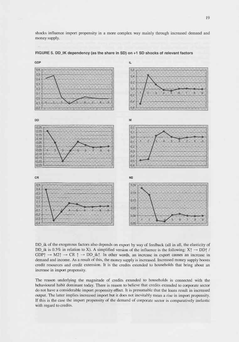
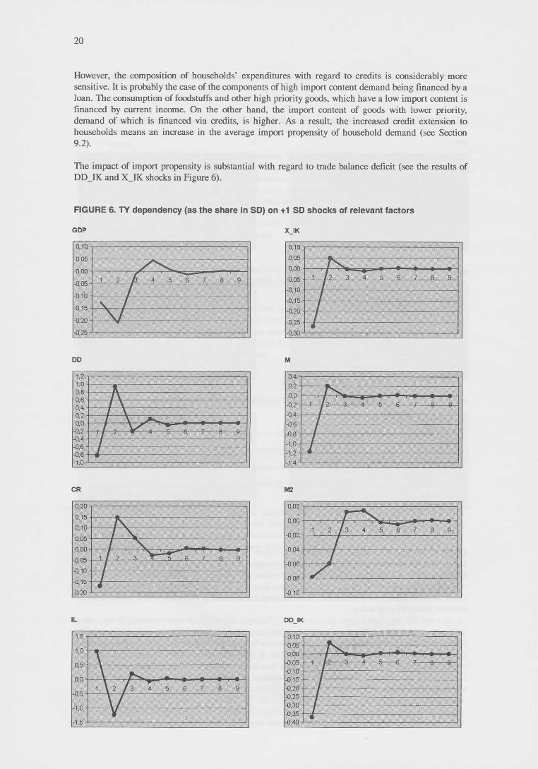
The impact of import propensity is substantial with regard to trade balance deficit (see the results of DD_IK and X_IK shocks in Figure 6).

FIGURE 6. TY dependency (as the share in SD) on +1 SD shocks of relevant factors

GDP X IK

DD M

CR M2

IL DD IK

The import propensity is an endogenous variable according to the structure of the model. Thus, import propensity is as if halfway down the road to the impact of exogenous factors on trade balance.

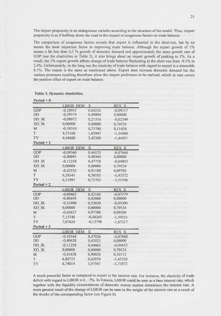
The comparison of exogenous factors reveals that export is influential in the short-run, but by no means the most important factor in improving trade balance. Although the export growth of 1% means a bit less than 0,5 % growth of domestic demand and approximately the same growth rate of GDP (see the elasticities in Table 3), it also brings about an import growth of peaking to 1%. As a result, the 1% export growth affects change of trade balance fluctuating in the short-run from -0.1% to 2.4%. Unfortunately, in the long run the elasticity of trade balance with regard to export is a miserable 0.1%. The reason is the same as mentioned above. Export does increase domestic demand but the various processes resulting therefrom allow the import preference to be realised, which in turn covers the positive effect of export on trade balance.

Table 3. Dynamic elasticities.

Period + 0LIBOR DEM X REX X

GDP -0,10915 0,64216 -0,09317DD -0,39574 0,48004 0,00000DD IK -0,08072 0,21516 -0,02349XD IK 0,00000 0,00000 0,70524M -0,38510 0,75700 0,11426T 4,53168 1,85947 -1,34460TYPeriod + 1

4,44680 2,42380 -1,44451

LIBOR DEM X REX XGDP -0,09360 0,44125 -0,07644DD -0,40691 0,40364 0,00000DD IK -0,12238 0,47758 -0,04803XD IK 0,00000 0,00000 0,70524M -0,42533 0,91188 0,09705T 6,28341 0,30183 -1,43372TYPeriod + 2

6,21891 0,72703 -1,51596

LIBOR DEM X REX XGDP -0,09463 0,42184 -0,07379DD -0,40659 0,42808 0,00000DD IK -0,12498 0,52820 -0,05200XD IK 0,00000 0,00000 0,70524M -0,42627 0,97388 0,09509T 7,13740 -0,56265 -1,59221TYPeriod + 3

7,07624 -0,13790 -1,67217

LIBOR DEM X REX XGDP -0,10164 0,47026 -0,07868DD -0,40628 0,42025 0,00000DD IK -0,11258 0,44663 -0,04425XD IK 0,00000 0,00000 0,70524M -0,41638 0,90026 0,10112T 6,80753 0,63070 -1,65320TY 6,74014 1,07567 -1,73872

A much powerful factor as compared to export is the interest rate. For instance, the elasticity of trade deficit with regard to LIBOR is 6...7%. In Estonia, LIBOR could be seen as a base interest rate, which together with the liquidity circumstances of domestic money market determines the interest rate. A more general result of the change of LIBOR can be seen in the weight of the interest rate as a result of the shocks of the corresponding factor (see Figure 6).

The impact of the credits extended to households is an order of magnitude less than the impact of interest rate. This effect seems to undervalue the actual one. It is conditioned by the partial nature of the model. Our simple model excludes the mutual adjustments of credit volumes and interest rates as in Estonia the increase of credit stock have been accompanied by the decline in the interest rates. As both variables are separated, the interest rate remains constant in the simulations of effects of the credit stock changes and vice versa. In real economy, contrary to our calculations, the growth of credit stock would have been accompanied by the decreased interest rates. Credits would have increased import, due to increase of domestic demand, what have lessened the effect in the trade balance. Thus we may presume that the impact of the credits is partly reflected in the simulated impact of interest rate.27.

The partial nature of the model accounts also for the simulated impact of interest rate, which probably exceeds the real effect. In the case of an increasing interest rate one should consider the decreasing credit extension and the declining import propensity as the factors that reduce the trade deficit.

The impact of M shock is of primary importance to the level of deficit. It is only rational since import decreases TY and increases GDP. Another issue, however, is how realistic it is to improve current account deficit by import shock that means setting up the import restrictions, in our present liberal economic framework.

The effects of DD and GDP are also considerable. The comparison of those variables points to the fact that the effect of DD is almost one order of magnitude larger. This is representative of one of the characteristic features of the Estonian economy (at least according to the model). Domestic demand is largely external supply oriented, whereas the increased demand can be characterised by an increased propensity to import and worsening deficit. Since domestic demand is import oriented, the role of domestic demand as an engine of economic growth is therefor smaller. This can be also seen in the impact of DD shock on GDP and M. A demand shock causes a change in the standard deviation for GDP of 0.4...0.6 and for import of 0.8. It is first and foremost the external demand that determines economic growth. For instance, the impact elasticity of GDP with regard to export equals 0.4... 0.6%.

13. Conclusions

• Monetary effects (that are the effects of interest rate, of credit and of money supply) are of considerable weight in determining the deficit level in short term. Monetary effects are on one hand connected with capital inflow (as to increased credit supply and resulting decline of interest rates) and on the other hand with the behaviour of financial sector which acts as an intermediary for foreign capital reaching the residents. Leaving aside the financial sector, the capital inflow is the factor of an utmost relevance for the current account. However, the capital inflow also has a marginal influence on the economic growth as it goes largely for financing external supply or for refinancing former obligations.

• The behaviour of the financial sector in mediating capital inflow is crucial for the trade deficit, since the high import content demand, first of all private consumption, during the intensive capital inflow in years 1996-1998 was financed through crediting by the financial sector. In brief, the results of simulation suggest that to improve the trade balance (the externally financed) crediting of households is to be cramped, reducing the use of external savings in financing the imports as the consumption/saving behaviour suggests that the Estonian residents are preferring consumption to saving.

27 The partial nature of the model accounts also for the simulated impact of interest rate, which probably exceeds the real effect. In the case of an increasing interest rate one should consider the decreasing credit extension and the declining import propensity as the factors that reduce the trade deficit.

• The increase of export is important when taking into consideration the aspect of trade balance convergence in the short-run. Yet the expanding export produces increasing incomes and demand, what mean (due to the very low substitutability between imported and domestic goods) growing imports.

• Deficit depends also to a great extent on subcontracting: the 1% decrease of its share will improve the balance with respect to GDP by 1.4%. To improve the trade balance the portion of subcontracting must be reduced and the (export) production has to be oriented, to an ever-greater extent, to the domestic inputs (if it is really possible).

14. References

Aghevli, B. B. - Sassanpour, C. (1991). Prices, Output, and the Trade Balance in Iran. Macroeconomic Models for Adjustment in Developing Countries, IMF.

Alexius, A. (1993). Effects of the Real Interest Rate and the Real Effective Exchange Rate on Demand. Monetary Policy Indicators. Sveriges Riksbank, June.

Arestis, P. -Howells, P. (1995). Changes in Income Distribution and Aggregate Spending: Constraints on Full-employment?. Review of Political Economy, vol 7:2.

Bruce, N., Purvis, D. D. (1984). The Specification and Influence of Goods and Factor Markets in Open-Economy Macroeconomic Models. Handbook of International Economics. Elsevier.

Dervis, K .- de Melo, J. - Robinson, S. (1982). General Equilibrium Models for Development Policy. Cambridge University Press.

Eesti Pank (1998). Newsletter No 8 (191), June 1998. Comments on the Estonian Preliminary Balance of Payments for the First Quarter of 1998.

Fisher, P., Whitley, J. (1998). Macroeconomic Models at the Bank of England. Paper for “The UK’s Major Macroeconomic Modelling Conference 1998”, London, January 8-9.

Fischer, S. (1986). Indexing Inflation and Economic Policy, MIT Press.

Goldstein, M. - Khan, M. S. Income and Price Effects in Foreign Trade (1984). Handbook of International Economics. Elsevier.

Gandolfo, G (1995). International Economics II. International Monetary Theory and Open-Economy Macroeconomics. Springer-Verlag.

Gandolfo, G. - Padoan, P. (1990). The Italian Continues Time Model. Theory and Results. Economic Modelling, April, 91-132.

Khan, M. S. - Knight, M. D. (1991). Stabilization Programs in Developing Countries: A Formal Framework. Macroeconomic Models for Adjustment in Developing Countries, IMF.

Kohler, G. (1996). Propensity to Import (100 countries), http://csf.colorado.edu/mail/pkt/96/dec96/010

Lamfalussy, A. (1963). Contribution a une theorie de la croissance en economic ouverte, Recherches Economiques de Louvain, 29, 715-734.

Lipschitz, L. (1991). Domestic Credit and Exchange Rates in Developing Countries - Some Policy Experiments with Korean Data. Macroeconomic Models for Adjustment in Developing Countries, IMF.

Laursen, S. - Metzler, L. A. (1959). Flexible Exchange Rates and the Theory of Employment, Review of Economics and Statistics, 32, 281-299.

Laxton, D. (1998); Isard, P.; Faruqee, H.; Prasad, E.; Turtelboom, B. MULTIMOD Mark III - The Core Dynamic and Steady-State Models. IMF Occasional Paper No 164.

Osang-Pereira (1997). Foreign Growth and Domestic Performance in a Small open Economy, Journal of International Economic, 1997, p 49-512.

Phylaktis, K. (1995). Capital Market Integration in the Pacific Region: An Analysis of Real Interest Rate Linkage. IMF WP/95/133.

Senhadji, A. (1997). Time-Series Estimation of Structural Import Demand Equations: A Cross- Country Analysis. IMF WP/97/132, October.

Senhadji, A. - Montenegro, C. (1998). Time Series Analysis of Export Demand Equations: A Cross- Country Analysis. IMF WP/98/149.

Sepp, U. (1996). Monetary Reform, Currency Board Arrangement and Inflation in Estonia. Proceedings of 5th Conference of the International Society for the Study of European Ideas, Utrecht, August 19-24.

Sepp, U. (1998). Export Growth and Trade Balance in Estonia (the paper for the 4th Conference on Financial Sector Reform in Central and Eastern Europe, Tallinn, April 24-26, 1998; published in Working Papers in Economics. Tallinn Technical University, No. 98/20).

Smets, F. (1997) Financial Assets Prices and Monetary Policy: Theory and Evidence. BIS WP 47, September.

Traks, K. - Männik, S. (1997). Eesti toiduained on kallinenud kaks korda. Äripäev 12.12.97.

Vaez-Zadeh., R. (1991). Oil Wealth and Economic Behavior: The Case of Venezuela, 1965-81. Macroeconomic Models for Adjustment in Developing Countries, IMF.

P E "fe3

CCCTI PAHVI I.QRAAMATl 1KOGLJ

rn 49<0<3,4