Embed Size (px)
Citation preview

FACTORS OF PERSONAL BANKRUPTCY: A CASE
STUDY OF MALAYSIA
BY
TAN ANN-YEW
A research project submitted in partial fulfillment of the
requirement for the degree of
MASTER OF BUSINESS ADMINISTRATION
(CORPORATE MANAGEMENT)
UNIVERSITI TUNKU ABDUL RAHMAN
FACULTY OF BUSINESS AND FINANCE
DEPARTMENT OF FINANCE
SEPTEMBER 2017

Factors of Personal Bankruptcy: A Case Study of Malaysia
ii
Copyright@2017
ALL RIGHTS RESERVED. No part of this paper may be reproduced, stored in a
retrieval system, or transmitted in any form or by any means, graphic, electronic,
mechanical, photocopying, recording, scanning, or otherwise, without the prior
consent of the authors.

Factors of Personal Bankruptcy: A Case Study of Malaysia
iii
DECLARATION
We hereby declare that:
(1) This postgraduate research project is the end result of my own and that due
acknowledgement has been given in the reference to ALL sources of
information be they printed, electronic, or personal.
(2) No portion of this research project has been submitted in support of any
application for any other degree or qualification of this or any other university,
or other institutes of leering.
(3) The word count of this research report is 20,122.
Name of Student: Student ID: Signature:
Tan Ann-Yew 16ABM00497 _____________
Date: 25th
August 2017

Factors of Personal Bankruptcy: A Case Study of Malaysia
iv
Acknowledgement
Thousands thanks to those who made this research project a success. First and
foremost, I would like to express my gratitude to my research supervisor,
Dr Zuriawati Binti Zakaria for her guidance and encouragement in the progress of my
research. Secondly, I would like to have a shout out of gratitude to my family who
gave me a chance to pursue my study. Without the support from them, I will not be
this far away from yesterday. They have been very supportive throughout my study
especially the time I faced any issue regarding my study, they will be telling me ‘You
can’ that pushed me this far away. Lastly, the classmates which we shared a lot on
research, they are the one who gave me advices and directions whenever I needed it.
It is a good feeling to work side by side with you all and thank you for all the supports
and help given.

Factors of Personal Bankruptcy: A Case Study of Malaysia
v
TABLE OF CONTENTS
Page
Copyright Page………………………………………………...............................……ii
Declaration………………………………….………………………………….……..iii
Acknowledgement…………………………………………………………………….iv
Table of Contents…………………………………………………………….…….….v
List of Tables………………………………………………………………….....…….x
List of Figures…………………………………………………………….….…….…xi
List of Abbreviations…………………………………………………….………..…xii
Preface……………………………………………………………………...…….…xiii
Abstract………………………………………………………………………...……xiv
CHAPTER 1 RESEARCH OVERVIEW………………………………………….….1
1.1 Introduction………………………………………………………………………..1
1.2 Research Background……………………………………………………...………1
1.3 Problem Statement…………………………………………………………...……4
1.4 Research Objective………………………………………………………….……..8
1.4.1 General Objective……………………………………………………………8
1.4.2 Specific Objectives…………………………………………………………..8
1.5 Research Questions………………………………………………..………………8
1.6 Hypothesis of the Study……………………………………………………..…….9
1.6.1.1 Unemployment rate………………………………………………………..9

Factors of Personal Bankruptcy: A Case Study of Malaysia
vi
1.6.1.2 Lending Rate……………………………………………………………..10
1.6.1.3 Divorce case……………………………………………………..……….10
1.6.2 Long-run versus short-run relationship…………………………………….11
1.6.3 Causal relationship……………………………………………………...….11
1.7 Significance of the Study……………………………………………………..….12
1.8 Chapter Layout……………………………………………………………….…..14
1.9 Conclusion………………………………………………………………………..15
CHAPTER 2 LITERATURE REVIEW………………………………………….….16
2.1 Introduction……………………………………………………………………....16
2.2 Review of Literature……………………………………………………...………16
2.2.1 Personal bankruptcy case……………………….…………………...…..…16
2.2.2 Unemployment rate………………………………….……………..………17
2.2.3 Lending rate……………………………………..……………….…………20
2.2.4 Divorce case………………………………………………………………..22
2.3 Theoretical Model…………………………….…………………………….……25
2.3.1 Personal bankruptcy case…………………………………………………..25
2.3.2Unemployment rate………………………………………………….….…..26
2.3.4Lending rate…………………………………………………………………27
2.3.4Divorce case…………………………………………………………..…….28
2.4 Proposed Theoretical Framework…………………………………………..……29
2.5 Hypothesis Development………………………………………………...………29
2.5.1 The unemployment rate and the personal bankruptcy case…………...……29
2.5.2 The lending rate and the personal bankruptcy case……………………...…30

Factors of Personal Bankruptcy: A Case Study of Malaysia
vii
2.5.3 Divorce case and the personal bankruptcy case……………………………30
2.5.4 Long-run versus short-run…….....................................................................31
2.5.5 Causal relationship…………………………………………………..……..31
2.6 Conclusion……………………………………………………………….……….32
CHAPTER 3 METHODOLGY………………………………………………..…… 33
3.1 Introduction………………………………………………………………………33
3.2 Data Collection Methods…………………………………………………………33
3.3 Data Analysis………………………………………………………………….…34
3.3.1 Ordinary Least Squares (OLS) ……………………………………………35
3.4 Diagnostic Checking…………………………………………………………..…36
3.4.1 Unit Root Test……………………………………………………………….…36
3.4.1.1 Augmented Dickey Fuller Test (ADF) ……………………………..……37
3.4.1.2 Philips-Perron Test (PP) …………………………………………………38
3.4.2 Normality test………………………………………………………………39
3.4.3 Multicollinearity Test………………………………………………………39
3.4.4 Heteroscedasticity………………………………………………….………40
3.4.5 Model Specification…………………………………………..……………41
3.4.6 Autocorrelation………………………………………………………..……42
3.5 Inferential Statistics………………………………………………………………43
3.5.1 R-Squared………………………………………………………………..…43
3.5.2 Adjusted R-Squared……………………………………………..…………44
3.5.3 F-test Statistic………………………………………………………………44
3.5.4 T-test Statistic………………………………………………………………45

Factors of Personal Bankruptcy: A Case Study of Malaysia
viii
3.6 Johansen Co-integration Test……………………………………………….……46
3.7 Vector Error Correction Model (VECM) …………………………………..……47
3.8 Granger Causality Test……………………………………………………...……48
3.9 Impulse Response Function………………………………………………...……49
3.10 Conclusion………………………………………………………………………50
CHAPTER 4 DATA ANALYSIS……………………………………………………51
4.1 Introduction………………………………………………………………………51
4.2 Diagnostic Checking………………………………………………………..……51
4.2.1 Unit root Test………………………………………………………………51
4.2.2 Multicollinearity …………………………………………………...………53
4.2.3 Heteroscedasticity………………………………………………….………55
4.2.4 Model Specification………………………………………………..………56
4.2.5 Normality Test…………………………………………………………...…57
4.2.6 Autocorrelation……………………………………………………………..58
4.3 Multiple Linear Regression Model………………………………………………59
4.3.1 Interpretation on Intercept and Independent Variables……………….……60
4.4 Inferential Analyses………………………………………………………………62
4.4.1 Interpretation on R2 and �̅�2
…………………………………………..…….62
4.4.2 F-test Statistic…………………………………………………………...….62
4.4.3 T-test Statistic………………………………………………………………63
4.4.3.1 Unemployment rate……………………………………………….…64
4.4.3.2 Lending rate……………………………………………………..…..65
4.4.3.3 Divorce case…………………………………………………………66

Factors of Personal Bankruptcy: A Case Study of Malaysia
ix
4.5 Johansen Cointegration Test…………………………………………………..…67
4.6 Vector Error Correction Model (VECM) …………………………………..……69
4.7 Granger Causality Test……………………………………………………...……71
4.8 Impulse Response Function…………………………………………………...…72
4.9 Conclusion……………………………………………………………………..…75
CHAPTER 5 DISCUSSION, CONCLUSION, AND IMPLICAITON……...………76
5.1 Introduction………………………………………………………………………76
5.2 Summary of Statistical Analyses………………………………………………....76
5.3 Discussion of Major Findings……………………………………………………78
5.3.1 Unemployment rate……………………………………………….……..…78
5.3.2 Lending rate………………………………………………………….….….80
5.3.3 Divorce case…………………………………………………………….….81
5.4 Implication of the study………….…………………………………………….…83
5.4.1Unemployment rate…………………………………………………………83
5.4.2 Lending rate…………………………………………………………….…..84
5.4.3 Divorce case……………………………………………………………..…85
5.5 Limitation of the Study…………………………………………………………..86
5.6 Recommendation for Future Research………………………………………..…87
5.7 Conclusion…………………………………………………………………….….88
References…………………………………………………………………………....90
Appendices…………………………………………………………………….……..96
Factors of Personal Bankruptcy: A Case Study of Malaysia
x
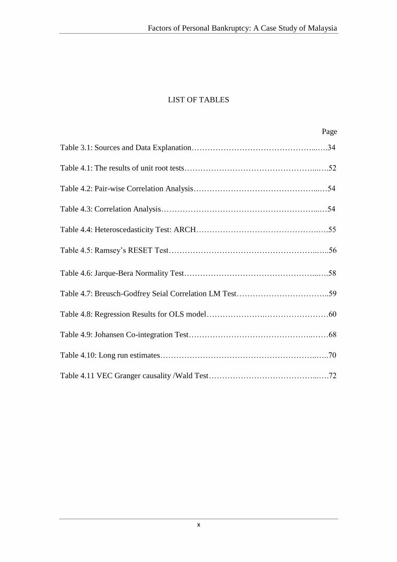
LIST OF TABLES
Page
Table 3.1: Sources and Data Explanation………………………………………...….34
Table 4.1: The results of unit root tests…………………………………………...….52
Table 4.2: Pair-wise Correlation Analysis………………………………………...…54
Table 4.3: Correlation Analysis…………………………………………………...…54
Table 4.4: Heteroscedasticity Test: ARCH……………………………………….….55
Table 4.5: Ramsey’s RESET Test………………………………………………..…..56
Table 4.6: Jarque-Bera Normality Test…………………………………………...….58
Table 4.7: Breusch-Godfrey Seial Correlation LM Test……………………………..59
Table 4.8: Regression Results for OLS model………………….……………………60
Table 4.9: Johansen Co-integration Test………………………………………..……68
Table 4.10: Long run estimates…………………………………………………..…..70
Table 4.11 VEC Granger causality /Wald Test…………………………………...….72

Factors of Personal Bankruptcy: A Case Study of Malaysia
xi
LIST OF FIGURES
Page
Figure 1.1: Household debt to GDP in Malaysia………………………………...……2
Figure 1.2: Personal Bankruptcy in Malaysia………………………………………....2
Figure 1.3: A comparison of unemployment rate and lending rate with
p.bankruptcy……………………………………………………………….5
Figure 1.4: Comparison of personal bankruptcy and divorce in Malaysia…………....7
Figured 2.1: Framework for the Factors of Personal Bankruptcy of Malaysia…...….29
Figure 4.1: Impulse reponse functions for 10 periods……………………………..…74

Factors of Personal Bankruptcy: A Case Study of Malaysia
xii
LIST OF ABBREVIAITONS
GDP Gross domestic product
MDI Malaysia Department of Insolvency
DOSM Department of Statistics Malaysia
BNM Bank Negara Malaysia
AKPK Agensi Kaunseling dan Pengurusan Kredit
U.S. United States
U.K. United Kingdom
FHA Federal Housing Association
OLS Ordinary Least Squares
DF Dickey Fuller
ADF Augmented Dickey Fuller Test
PP Philips-Perron Test
VIF Variance Inflation Factor
ARCH Autoregressive Conditional Heteroscedasticity
RESET Regression Equation Specification Error Test
BLUE Best, Linear, Unbiased, Estimator
VAR Vector Autoregressive
VECM Vector Eror-Correction Model
IR Impulse Response Function
SIC Schwarz Info Criterion
AIC Akaike Information Criterion
ECT Error Correction Term

Factors of Personal Bankruptcy: A Case Study of Malaysia
xiii
PREFACE
This research is submitted in as a fulfillment of the requirement for the pursuit of the
Master Degree in Business Administration (Corporate Management). This research is
focusing on the determinants of the personal bankruptcy case in Malaysia by using the
independent variable of the unemployment rate, lending rate, and divorce case. The
increasing trend of the personal bankruptcy case in Malaysia has raised the concern of
the policy makers and the researchers as this will essentially become a stumbling
block for Malaysia to become a high-income status nation by 2020. Even the past
researchers have identifies the factors driven by the high personal bankruptcy case in
Malaysia was due to the credit card debt, car loan, and insufficient knowledge in
personal financial management. Based on all these identified factors, the policy maker
has designed some policy in curbing this problem. However, the personal bankruptcy
cases are kept touching record high level in every year. This has raised the question
that whether there are other important potential variables being ignored by the
researcher and the policy maker. The details of the research findings, policy
implication, limitation of this research, and the recommendations for the future
researcher will be discussed further in this research paper.

Factors of Personal Bankruptcy: A Case Study of Malaysia
xiv
ABSTRACT
Personal bankruptcy is one of the main concerns by the policy maker in nowadays.
The reason being is the increasing trend of the personal bankruptcy case in Malaysia
will essentially become a stumbling block for Malaysia to become a “high-income
status nation” by 2020. In Malaysia, in fact, the factors lead to the personal
bankruptcy has been extensively and the policy maker also has introduced some
policy in curbing this problem. However, the problem of the personal bankruptcy is
still kept increasing from year to year and this has raised the interest to study what is
some of the possible relevant factors lead to the personal bankruptcy has been ignored
by the researchers and the policy makers. With the hope that the identification of
these relevant factors can help the policy maker to come out some new policy which
can be more effective to control the personal bankruptcy case in Malaysia. In this
research, will study the factors lead to the personal bankruptcy case in Malaysia by
incorporating the factors of the unemployment rate, lending rate, and divorce case.
The study period starts from 1985 to 2015 with a total 31 observations. In this study i)
Ordinary Least Square (OLS) multiple regression models has been employed to study
the relationship of the unemployment rate, lending rate, and divorce case towards the
personal bankruptcy case. The results show all these independent variables are
significant. ii) Johansen cointegration test has been tested to investigate the existence
of the long-run or short-run relationship in the model. Subsequently, VEC model is
being employed to examine how the model coincided to the long-run relationships
while also enabling the short-run adjustment dynamics. Lastly, the Granger causality
has been tested to identify the causal relationship between the variables.

Factors of Personal Bankruptcy: A Case Study of Malaysia
1 of 140
CHAPTER1: RESEARCH OVERVIEW
1.1 Introduction
The personal bankruptcy case in Malaysia are kept increasing ever since the 1980s
until the mid of 2010s. This study is designed to study the factors to influence the
personal bankruptcy case in Malaysia. The details about the idea to generate this
research will be discussed further in this chapter. Hence, the research objectives
and questions about the factors lead to the personal bankruptcy have been
generated. This research will develop the hypothesis of study i) To identify the
relationship between the personal bankruptcy case and the unemployment rate,
lending rate, and divorce case in Malaysia. ii) To identify the existence of a
cointegration relationship in the model. iii) To identify the causal relationship
among the variables. Lastly, the significance of study will be included in this
chapter.
1.2 Research Background
Malaysia, one of the fastest growing economies in Asian countries which aim to
become a “high-income status” nation by 2020 has to deal with one of the primary
obstacles to achieving this vision, which is the climbing of the personal
bankruptcy rate. According to Cheng, Wei, Rajagopalan and Hamid (2014),
Malaysia has the highest personal debt among 14 Asian economies. As shown in
Figure 1.1, the household debt to GDP in Malaysia has jumping to 89 percent of
gross domestic product (GDP) in 2015 from around 33 percent in 1997. Therewith,
the climbing record high to 89 percent of GDP in 2015 has surpassed Thailand
which boasted the highest household debt in Southeast Asia.

Factors of Personal Bankruptcy: A Case Study of Malaysia
2 of 140
Figure 1.1: Household debt to GDP in Malaysia
Source: Bank Negara Malaysia (BNM, 2015)
Based on the information provided by Malaysia Department of Insolvency (MDI),
the bankruptcy petition can be applied either by the debtors or the creditors as
long as the outstanding debt amount is more than RM 30,000.
Figure 1.2: Personal Bankruptcy in Malaysia
Source: Department of Statistics Malaysia (DOSM, 2015)
0
20
40
60
80
100
1997 2000 2003 2006 2009 2012 2015
Household debt to GDP
Household debt to GDP (%)
0
5,000
10,000
15,000
20,000
25,000
1985
1987
1989
1991
1993
1995
1997
1999
2001
2003
2005
2007
2009
2011
2013
2015
Case
Personal Bankruptcy Case
P.Bankruptcy

Factors of Personal Bankruptcy: A Case Study of Malaysia
3 of 140
Based on Figure 1.2 displays the evolution of the personal bankruptcy case in
Malaysia from the year 1985 and 2015. In general, the personal bankruptcy has
an upward trend from the 1980s to 2010s. There is a notable increase in a number
of personal bankruptcies in the Post-Asian Financial Crisis of 1997 and the Post-
Global Financial crisis of 2007-2008. Specifically, the bankruptcy cases have
climbed by 114% from the year 1993 and 2005. Meanwhile, the personal
bankruptcy cases have climbed by 68% from the year 2007 and 2014. An
explanation given by Sutthirak and Gonjanar (2012) to explain the post-financial
crisis effect is the individual was stuck in their liquidity problem due to a huge
loss on their capital investment.
According to a research done by MDI, in 2007 there were around 0.049% of a
population of 26.8 million declared bankruptcies. Specifically which is around 37
Malaysian going bankruptcies in every single day. Surprisingly, this figure was
kept climbing until 2014, where there were around 0.075% of a population of
29.9 million declared bankruptcies. Specifically, which is around 62 Malaysian
declaring bankruptcies in every single day. In other words, the personal
bankruptcy reported in every single day has been increased by 68% in the past 7
years and yet this figure is still climbing until today (Carvalho and Hamdan,
2015).
With the increasing number of bankruptcy cases reported from year to year it is
noticed that the young in nowadays are tend to over borrowing which has beyond
their ability to handle the debts level. Based on the findings of D'Alessio and
Iezzi (2013), the composition of the heavy household debt burdens is mainly
contributed by housing loans, car loans, and others. Currently, the bad debts in
local banks are still low, yet it is notable an increasing trend to declare
bankruptcy for those under age of 35. To the extent that financial difficulties of
an individual would reduce personal consumption. Besides that, another problem
for Malaysia's economy on top of low commodity prices, a battered currency and
a political crisis (Carvalho and Hamdan, 2015).
Factors of Personal Bankruptcy: A Case Study of Malaysia
4 of 140
Furthermore, the economics of Malaysia is mainly supported by domestic
(private) consumption, as the growth of private consumption has been slowing,
and if that continues, Malaysia's growth rates could be hit. In fact, in Malaysia,
the speed of debt accumulation by the households is much faster than the speed
of their incomes growth. As a result, this will increase the likelihood of
repayment difficulties when the credit cycle turns. The default on debt
repayments had brought negative impact on the banking industry. It was
considered as non-performing loan and a cost to the banks. Banks put the
bankruptcy cost in their income statement as provision for loan losses (Chow,
2015).
1.3 Problem Statement
The increasing trend in the personal bankruptcy is always the major concern of
the policy maker (Thomas and Michael, 2002). In Malaysia, the research about
the factors lead to the personal bankruptcy has been extensively studied where
the factors were mainly contributed by the non-performing loan from car loans,
personal loans, credit card debt, and insufficient knowledge in personal financial
management (Cheng et al., 2014; Selvanathan, Krusnan, and Wong, 2016; and
Zamzamir, Jaini, and Zaib, 2013). Based on the identified factors, the policy
maker has come out some measures to control the personal bankruptcies problem.
For instance, there are two agencies being set up by the Bank Negara Malaysia
(BNM) which are the Malaysia Department of Insolvency (MDI) and Agensi
Kaunseling dan Pengurusan Kredit (AKPK). The mission of MDI is to facilitate
and control the bankruptcy problem while the AKPK is acting like a financial
consultant in providing financial information and debt rescheduling plan for
those facing financial problems. Meanwhile, BNM has required all commercial
banks to tighten their rules in borrowing loans and issuing credit cards (“New
Measures on,” 2006 and “Malaysia tightens household,” 2013).

Factors of Personal Bankruptcy: A Case Study of Malaysia
5 of 140
However, the increasing number of bankruptcies cases from the year 2007 and
2014 showing that the agencies are not effective in curbing the problem. This has
come to the question that whether there is other major factors that may lead to the
increasing trend in the personal bankruptcy. According to a research done by
Garrett (2007) revealed that the rapidly increase in the number of consumer
bankruptcy in the United States (US) was generally caused by debt overload and
the impact of unexpected negative shocks such as divorce, unemployment, and
medical expenses. Besides that, a research done by Jappelli, Pagano and Maggio
(2008) by incorporating macroeconomic variables to study the relationship with
personal insolvency. The authors conclude that the climbing of interest rate and
the unemployment rate has resulted in climbing of personal insolvency.
Figure 1.3: A comparison of the unemployment rate and the lending rate with the
personal bankruptcy
Source: Department of Statistics Malaysia (DOSM, 2015)
Based on the research findings of Garrett (2007) and Jappelli et al. (2008) have
created an interest to investigate whether the unemployment rate, the lending rate,
and divorce case are the factors to influence the climbing of the personal
bankruptcy case in Malaysia. Figure 1.3 displays the trends between the
unemployment rate, lending rate, and the personal bankruptcy case in Malaysia
from the year 1985 and 2015. Based on the graphical approach shows there is a
0.00
2.00
4.00
6.00
8.00
10.00
12.00
14.00
0
5,000
10,000
15,000
20,000
25,000
1985
1988
1991
1994
1997
2000
2003
2006
2009
2012
2015
Perc
en
tage
P.Bankruptcy
Unemployment rate
Lending rate

Factors of Personal Bankruptcy: A Case Study of Malaysia
6 of 140
negative relationship between the unemployment rate and the personal
bankruptcy case. From the theoretical point of view, unemployment and the
personal bankruptcy should be positively correlated. However, a possible reason
can explain why the unemployment rate was dropping significantly in the mid-
1980s was due to the rapid economy growth in that period. The rapid economic
growth in Malaysia has demanded a lot of workers until the labour are being
shortage in the market. This explains why the unemployment rate fell from about
8 percent in 1987 to 5 percent in 1990 (Felker and Jomo, 2013).
The lending rate, on the other hand, shows an upward trend from the year 1985
and 2015 and it has a positive relationship with the personal bankruptcy case.
The lending rate was started to increase from about 4.5 percent in 1985 and
reached about 12 percent in the mid-2000s. The reason for the steady climbing of
the lending rate was due to the steady climbing of the market interest rate in
order to stabilize the inflation rate in Malaysia during the rapid economic growth
since the mid-1980s (Felker and Jomo, 2013). When there is a change in the
lending rate will directly affect the cost of servicing the debt. Likewise, an
increasing lending rate means an increasing cost of debt and therefore, a higher
the personal bankruptcy case. Besides from the macroeconomic variables
(unemployment rate and lending rate) has been discussed earlier, the divorce rate
is suspected to be another important factor would influence the individual
insolvency. In fact, the divorce rate in Malaysia has become one of the serious
concerns as the divorce cases reported is keep climbing from year after year as
shown in Figure 1.4.

Factors of Personal Bankruptcy: A Case Study of Malaysia
7 of 140
Figure 1.4: Comparison of personal bankruptcy and divorce in Malaysia
Source: Department of Statistics Malaysia (DOSM, 2015)
Figure 1.4 displays the trends between the personal bankruptcy case and divorce
case in Malaysia from the year 1985 and 2015. Based on the graphical approach
shows there is a positive relationship between the personal bankruptcy case and
divorce case. This has created a question whether the increasing of divorce case
is one of the important factors resulted the increasing of the personal bankruptcy
case in Malaysia. Based on a research revealed there were 56,760 divorces were
recorded in 2012, which equivalent to a marriage is breaking down every 10
minutes. Divorce could bring more financial distress to one of the parties. This
includes the cost of keeping up the 2 separate household such as alimony and
child payment support (Boon, 2014). Up to date, as to author knowledge in
Malaysia, there is no researcher incorporating the variables of the unemployment
rate, lending rate, and divorce case into consideration to study the relationship
with the personal bankruptcy. This has raised an interesting issue to study
whether all these variables are an important factor leading to high personal
bankruptcies in Malaysia.
0
10,000
20,000
30,000
40,000
50,000
60,000
70,000
80,000
90,000
1985
1987
1989
1991
1993
1995
1997
1999
2001
2003
2005
2007
2009
2011
2013
2015
Case
Divorce
P.Bankruptcy
Factors of Personal Bankruptcy: A Case Study of Malaysia
8 of 140
1.4 Research Objective
In this research, general objective and specific objectives are stated in order to
identify the goals for this research project.
1.4.1 General Objective
To investigate the factors of the personal bankruptcy case in Malaysia.
1.4.2 Specific Objectives
a) To identify the relationship between the personal
bankruptcy case and its independent variables which are the
unemployment rate, lending rate, and divorce case.
b) To identify the existence of a cointegration relationship in
the model.
c) To identify the causal relationship among the variables.
1.5 Research Questions
a) What is the relationship between the personal bankruptcy case and its
independent variables which are the unemployment rate, lending rate, and
divorce case?
b) Is there any cointegration relationship in the model?
c) What is the causality pattern among all the variables?
Factors of Personal Bankruptcy: A Case Study of Malaysia
9 of 140
1.6 Hypothesis of the Study
1.6.1.1 Unemployment Rate
H0a: Unemployment rate does not have a significant relationship
with the personal bankruptcy case.
H1a: Unemployment rate have a significant relationship with the
personal bankruptcy case.
Based on Warren (2003) proposed that the reasons of the climbing
in the personal bankruptcy case of a country is due to the adverse
events in the labour market. For instance, a job loss and salary
reduction during a bad economic condition. This is because when
there is a steady income is being earned, individuals would able to
make their monthly debt repayment easily and on time. This could
signify the use of credit cards or personal loans is not a necessity.
However, during unemployment, income will stop, families are
forced to quickly spend down their accrued saving balances on
everyday living expenses. When savings are depleted, getting loans
to fund their life has become a necessity to support the current
living expenses. This can result in serious financial issues for those
who do not have an income to make their debt repayment. The
unemployment then leads to outstanding personal loan debts that
end up in default, perpetuating financial concerns even further.

Factors of Personal Bankruptcy: A Case Study of Malaysia
10 of 140
1.6.1.2 Lending Rate
H0b: Lending rate does not have a significant relationship with
the personal bankruptcy case.
H1b: Lending rate have a significant relationship with the personal
bankruptcy case.
Based on Jappelli et al. (2008) proposed that the increase in interest
rate is always associated with a higher personal bankruptcy rate. In
a situation where consumers are having high debt level due to the
financial crisis or economic recession followed by sharp rising
interest rate adjustment will lead to more consumers to declare
bankruptcy. This is because the rising interest rate will further
increase the burden on them to make debt repayment and as a
consequence higher bankruptcy reported. Therefore, this study
proposes that there is a significant relationship between the personal
bankruptcy and the lending rate.
1.6.1.3 Divorce case
H0c: Divorce case does not have a significant relationship with
the personal bankruptcy case.
H1c: Divorce case have a significant relationship with the personal
bankruptcy case.
Based on Poortman (2000), divorce can create financial distress on
both partners in a number of ways. Firstly, the primary cost after
divorce, for example, child support payments, education fees, and

Factors of Personal Bankruptcy: A Case Study of Malaysia
11 of 140
alimony. All these costs can easily drive up the financial burden to
one of the parties. As results, this study proposes that there is a
significant relationship between the personal bankruptcy case and
divorce case.
1.6.2 Long-run versus short-run relationship
H0: There is no cointegration relationship in the model.
H2: There is a cointegration relationship in the model.
Johansen Cointegration test will be used in order to identify
existence of a cointegration relationship in the model. If the model
does not have a cointegration relationship then this study will
employ a short-run model (Vector autoregressive) model.
Conversely, if there is a cointegration relationship in the model, a
long-run model (Vector Error Correction) will be employed in this
study (Gujarati and Porter, 2009).
1.6.3 Causal relationship
H0: Xt does not Granger cause Yt.
H3a: Xt does Granger cause Yt.
H0: Yt does not Granger cause Xt.
Factors of Personal Bankruptcy: A Case Study of Malaysia
12 of 140
H3b: Yt does Granger cause Xt.
The lag length involved, distributed, and autoregressive models has
raise the issue of causality in the economic variables. This is
because the finding in the OLS only can tell the existence of the
relationship between the variables where it does not prove any
causality or the direction of influence towards the dependent
variable. This is where the Granger causality test comes in to fill up
this gap. For instance, a variable Xt is said to Granger cause Yt, if
Yt can be predicted with greater accuracy by using past values of
the Xt variable rather not using such past values. Ceteris paribus
assumption (Gujarati and Porter, 2009).
1.7 Significance of the Study
Conceptually, when an individual is facing insolvency and turned out to declared
bankruptcy, in fact, this can benefit the economy of a country. The logic behind is
that, during the bankruptcy process, an individual can rebuild his/her credit record
if the outstanding debts of the debtors are discharged without any future obligation.
With this, can encourage an individual in spending and borrowing which is good
for the economy. Nevertheless, if they are increasing number of people filing for
bankruptcy at the same time can adversely affect the economy (Dobbie and Song,
2013). Thus, in this research will focusing on the factors that affect the personal
bankruptcy is mainly contributed to the policy makers, investors, and consumers.
After the difficult periods of the Asian Financial Crisis in the 1997 and the global
financial crisis in the 2009, the policy makers has introduced a number of rules
and regulations to enhance the local banking structure as well as the financial
market (Barth, Caprio, and Levine, 2013). By having a better understanding of the

Factors of Personal Bankruptcy: A Case Study of Malaysia
13 of 140
factors that lead to personal bankruptcy may help the policy makers to develop a
better policy to curb the increasing number of personal bankruptcy case. For
instance, if the lending rate is one of the significant variables to influence personal
insolvency, subsequently, the policy maker may control the lending rate of the
banking and financial institutions to ensure it is at the optimum level which will
not significantly increase the debt burden of the consumer. Similarly, the policy to
stabilize the unemployment rate and divorce case is another concern by the policy
maker which can allow to stabilize the personal bankruptcy of a country.
Besides that, this research tends to provide useful information for the investor to
make their investment decision making. According to Buehler, Kaiser, and Jaeger
(2012), a high personal bankruptcy rate of a country may always indicate a
country is facing a poor economic condition. Thus, based on the personal
bankruptcy rate of a country can actually signify to the investors about the actual
economic performance of a country before they invest in the country. Moreover,
for those bankruptcies personal might face difficulty in applying for new credit
and even looking for new jobs. Thus, if consumers have the personal financial
management knowledge can actually have a wise financial plan which can
effectively in preventing them from filing bankruptcy. Additionally, the financial
knowledge can allow the consumer to understand which type of lending rate
(fixed and floating) is actually suited for them when they are about to borrow
loans from the banking and financial institutions. With this can actually reduce the
chances of an individual to file for bankruptcy.

Factors of Personal Bankruptcy: A Case Study of Malaysia
14 of 140
1.8 Chapter Layout
This research project contains five chapters and they will be presented as follow:
Chapter 1: In Chapter 1, will provide an overall concept of the research project. It
contains research background, problem statement, research objectives (general
and specific), research questions, hypotheses as well as significant of the study.
Chapter 2: In Chapter 2, this chapter will discuss about the literature review on
personal bankruptcy form the previous researchers. It covers the empirical testing
procedures and proposed theoretical framework.
Chapter 3: In Chapter 3, this chapter determines the research methodology that
used to carry out the research. It shows the ways to conduct the research which
include data collection methods and data analysis.
Chapter 4: In Chapter 4, this chapter will interpret the research findings
corresponding to the research questions and hypotheses are discussed in detail.
This study interprets and analyses the data collected from the Department of
Statistics Malaysia (DOSM).
Chapter 5: In Chapter 5, this chapter provides an overall conclusion based on the
research project, including the summary of statistical analyses, discussion of
major findings, implications and limitations of study as well as recommendations
for future research.

Factors of Personal Bankruptcy: A Case Study of Malaysia
15 of 140
1.9 Conclusion
In conclusion, in Chapter 1 will briefly explain the general concept of the study
towards the personal bankruptcy in Malaysia. Firstly, this study is designed to
investigate the significant relationship between the independent variables
(unemployment rate, lending rate, and divorce case) and the dependent variable
(personal bankruptcy case). This research aims to investigate whether these
independent variables would have a positive or negative relationship with personal
bankruptcy case. The previous researchers found that there are several factors will
lead to personal bankruptcy by conducting primary data research. However, this
study chooses this few independent variables to conduct the research as they have
proved a stronger relationship with personal bankruptcy. Secondly, the existence
of a cointegration relationship in the model will be examined followed by the
examination of the causal relationship among the variables. The evidence and
justification will be discussed in the following chapter.

Factors of Personal Bankruptcy: A Case Study of Malaysia
16 of 140
CHAPTER 2:LITERATURE REVIEW
2.1 Introduction
In this chapter, a brief review of the factors (unemployment rate, lending rate, and
divorce case) leading to the personal bankruptcy case from different researchers
have been extensively studies. The research objective is to identify the factors of
the personal bankruptcy in Malaysia. Additionally, the technique, equations, and
models used by different researchers will be discussed in this chapter.
2.2 Review of Literature
2.2.1 Personal bankruptcy case
Personal bankruptcy is a type of debt solution for those people who is no
longer has the ability to pay back their debts in a reasonable time.
Basically, the personal bankruptcy can be divided into voluntary and
involuntary. Voluntary bankruptcy also known as “petitioning for
bankruptcy” is where an individual knowing he/she no longer has the
ability to pay his/her debts and therefore, file for bankruptcy. Involuntary
bankruptcy, on the other hand, is where the creditors taking a legal
bankruptcy proceedings to sue an individual for bankruptcy (Irby, 2017).
In Malaysia, any individual who is unable to pay a minimum debt amount
of RM 30,000 will be suing by the creditor to file for bankruptcy.

Factors of Personal Bankruptcy: A Case Study of Malaysia
17 of 140
2.2.2 Unemployment rate
The unemployment rate is one of the common macroeconomic variables
where the researchers, for instance, Deng, Quigley, and Van Order (2000);
also prefer to incorporate to study the relationship with personal
bankruptcy. This is due to the fact that from the theoretical point of view
unemployment should be statistically significant and positively influence
the personal bankruptcy filing. This is because when an individual has
loss of job, he/she can no longer meet its obligation to service their debts
such as student loan, car loan, and houses loans. As a result, he/she has to
file for bankruptcy and financial restructuring.
According to Hendershott and Schultz (1993); Deng, Quigley, and Van
Order (2000) in the studies of bankruptcy decision by incorporating the
macroeconomic factors, such as the unemployment rate. The findings
have consistent results to shows that unemployment is significant and
positively to influence the personal bankruptcy filing in their study. For
instance, Hendershott and Schultz (1993) study the foreclosures on the
federal housing association (FHA) single family mortgages insured from
the year 1975 and 1987. They found that the unemployment rate and the
book value of borrower equity are statistically significant to influence an
individual insolvency. In their study mentioned that unemployment has
forced the borrowers no longer has the ability to service its home loan
obligation. In this case, they are actually forced to sell the house and
move to another place. However, the moving decision actually increases
the likelihood of default due to the fact that the moving cost is actually
unable to deter from default. Furthermore, the decision to sell the house
urgently can reduce the effective equity in the house.
Nevertheless, the studies of Fay, Hurst, and White (2002) have failed to
show unemployment is a significant variable in the studies. Thus, the
Congressional Budget Office has pointed out that the empirical studies do

Factors of Personal Bankruptcy: A Case Study of Malaysia
18 of 140
not have a consistent result to prove that the macroeconomic variables
(unemployment) are significant to affect the filing rate. However, by
using the surveys of bankruptcy filers do have a consistent result to show
that unemployment is a significant factor in the decision of personal
bankruptcy.
According to a survey done by Sullivan, Warren, and Westbrook (2000)
in analysing a survey study of 1,991 bankruptcy filings have found that
the unexpected adverse events (such as unemployment, divorce, health
problems, and medical debts) are the major causes lead to the climbing in
bankruptcy filings in the United States. The findings from the survey
show that there is 67.6 percent of the filers claim that loss of the job is the
main reason for them to declare bankruptcy where these adverse events
have eventually creates an income shock. The loss of income or high
expenses would influence the debt repayment ability and thus, forcing
them to declare bankruptcy. Similarly, this statement is also supported by
Hetes-Gavra, Avram and Avram (2016) where they study among a
sample size of 2,000 bankruptcy filers in Europe also found that there is
20 percent of the filers claims that there were filing for bankruptcy due to
loss of job.
Meanwhile, other researchers have studies on the determinants of the
personal bankruptcy by using time series data. Grieb, Hegji, and Jones
(2001) study the macroeconomic factors and consumer behavior on the
personal bankruptcy via credit card defaults in a sample period from the
year 1981 and 1999. The finding show that the unemployment leads to
the climbing of credit card default rates due to the card user is relying on
the credit card to maintain the autonomous spending. As a result, the
credit card default has become a trigger point for the card user to file for
bankruptcy in the United States.

Factors of Personal Bankruptcy: A Case Study of Malaysia
19 of 140
Agarwal, Liu and Mielnicki (2003) study the effect of unemployment on
consumer bankruptcy by using the credit card data from the year 1995
and 2001 on 700,000 customers. The findings show that country
unemployment is critical in determining the consumer bankruptcy. The
study of Dick and Lehnert (2010) study the U.S. credit supply and rising
bankruptcy rate in the U.S. covering the sample period from the year
1981 and 1999. The findings show that the unemployment rate is
statistically and positively significant to affect personal bankruptcy.
Specifically, a 1 standard deviation increase in the unemployment rate
will increase the personal bankruptcy by 27 percent.
On the other hand, Gross and Souleles (2002) using the bank account
level quarterly data from the year 1995 and 1997 to conduct an empirical
study of the demand for unsecured credit and its impact on consumer
bankruptcy. They adopt a duration model to estimate the importance of
the different variables in predicting the default. Specifically, they estimate
the risk effects on default, age, macroeconomic shock and changes in the
costs of default. They draw a conclusion that risk effects, macroeconomic
shock, and cost of default are statistically significant to influence the
consumer default. Nonetheless, the macroeconomic variable (state
unemployment) is failed to show significant impact on consumer
bankruptcy. The authors explain that the unemployment is insignificant in
their study could be due to their sample period does not have enough
variation in unemployment.
Since, most of the researchers also found that the unemployment is a
statistically and positively variable to influence the personal bankruptcy
in their studies. Thus, in this research, it is expected the unemployment
variable is statistically and positively to influence the personal bankruptcy
case.

Factors of Personal Bankruptcy: A Case Study of Malaysia
20 of 140
2.2.3 Lending rate
Nominal interest rate is part of the monetary policy where the central
bank will revise the nominal interest rate on a quarterly basis. This would
forms a reference rate to adjust the lending rate by all the banking and
financial institutions. In other words, depending on the economic
performance of a country, the central bank can adjust the nominal interest
rate of a country to achieve a certain economic objective (Blanchard and
Johnson, 2013). For instance, the interest rate will be adjusted downward
to boost the economic growth via a lower real interest rate. A lower
interest rate which means a lower lending rate which could make
borrowing more attractive due to cheaper cost to serve the debts. Besides
that, a lower interest rate means lower return from the savings in the bank
which could reduce the incentive of saving yet increase the incentive of
borrowing. This in turns will increase the money supply in the market to
achieve the economic driven objective as well as to drives up the inflation
(Blanchard and Johnson, 2013).
However, bear in mind that as the economy becomes over heated, a
higher inflation rate will then followed by an increase of market interest
rate. This might increase the burden of creditors who are holding a high
level of floating loan debts. In this case, a higher cost of debt will increase
the number of people to file for bankruptcy since they have no way to
service the debt. This statement is supported by the study of Igor,
MacGee, and Tertilt (2010). The authors study the personal bankruptcy in
the United States from the year 1970 and 2004 by employing a
heterogeneous agent life-cycle model to evaluate how the changes in
uncertainty (income shocks, expense uncertainty) and credit market
environment (lending rate, transaction cost, and credit rating) can affect
the bankruptcy filing decision. The finding shows that the changes in
uncertainty cannot account quantitatively for the rise in bankruptcies.

Factors of Personal Bankruptcy: A Case Study of Malaysia
21 of 140
However, the changes in credit market environment are the main force
driving the rise in filings for bankruptcy.
Meanwhile, this statement is also supported by Jappelli et al. (2008). The
authors study the effect of macroeconomic variables (interest rate, lending
to households, cyclical indicators, and institutional variables) on personal
bankruptcy in 11 European countries by using Vector autoregressive (VA)
model. The result shows that the increasing interest rate and the
unemployment rate will lead to higher personal insolvency rate.
Additionally, during economic shocks or sharply rising in interest rate
also would significantly drive up the personal debt level. Moreover, other
researchers also show that the lending rate has a significant relationship
with consumer debt. When the lending rate increases, the cost of credit
card debt payment, hire-purchase loan, and personal loan also will
increase. This will become a significant financial burden for the
borrowers.
Conversely, when the lending rate decreases, which means consumers are
easier to settle their monthly debt obligations. This scenario was proven
by the research conducted by Katz (1999) in the United States. The author
studies the effect of the lending rate and consumer debt towards
insolvency. The finding shows that the number of personal bankruptcy
cases filling in 1993 and 1994 was declined followed by the dropping of
lending rate. In contrast, the number of bankruptcy cases filling was
increased in the late 1994 and 1995 due to the sharply increases of
lending rate. Meanwhile, Durkin and Staten (2012) also have the same
finding where the increasing nominal interest rate has resulted in climbing
of bankruptcy case being reported.
However, based on the research done by White (2010) has a contrary
point of view. The author studies the relationship between the
macroeconomic factors and the personal insolvency case of United

Factors of Personal Bankruptcy: A Case Study of Malaysia
22 of 140
Kingdom (UK) from the year 1975 and 2008. The finding shows that the
climbing of insolvency rate in the early 1990s was associated with an
increase in the unemployment rate. Nevertheless, the accumulation in
household credit and insolvencies was associated with falling interest
rates. The result shows that the real lending rate declined from 4.3% in
1997 to 1.8% in 2005. The low cost of borrowing in this period has lead
to increasing number of borrowers borrowing the loan and therefore,
increasing number of insolvency cases being reported from year to year.
This statement is also supported by Zywicki (2005) and Dell'Ariccia, Igan,
and Laeven, (2008) where they also find similar findings where the
decreasing in nominal interest rate is one of the factors resulted in higher
insolvency rate.
In conclusion, a majority of the researchers also found that the lending
rate is statistically significant and positively to influence the personal
bankruptcy case in their studies. However, a minority of the researchers
found that the lending rate is statistically significant yet it will negatively
to influence the personal bankruptcy. Thus, it is expected the lending rate
variable also will be statistically significant in these research yet the
relationship (positive or negative) towards the personal bankruptcy case is
yet to explore in this research since a different researchers has a different
findings in their research.
2.2.4 Divorce case
The climbing divorce case is becoming one of the primary concerns by
the policy makers and researchers as the climbing divorce case has a
notable effect on the climbing in the personal bankruptcy case of a
country. The reason being for divorce can be related to personal
insolvency is due to the fact that divorce does entail financial costs. After
divorce, regardless is a man or a woman also would results in a

Factors of Personal Bankruptcy: A Case Study of Malaysia
23 of 140
substantial decline in household income which would increase the
likelihood of living on social welfare or falling into poverty (Jarvis and
Jenkins, 1999; Duncan and Hoffman, 1985; Burkhauser and Duncan,
1989; Holden and Smock, 1991; Smock, 1994; Poortman, 2000).
According to Francis (2005), an economic report to investigate the impact
of household income after a divorce of the United States has been studied.
The report shows that the household income has fallen by 40% to 45% for
children whose parents divorce and remain divorced for at least 6 years.
Whereby, the food consumption for a divorced family also has reduced by
17% as compared to a non-divorce family. An explanation given by a
divorced family is due to the absence of a second parent in a variety of
ways that help mitigate some of the financial cost. Meanwhile, Edmiston
(2006) study in analyzing the new perspective of bankruptcy filing rates
in the United States from the year 1970 and 2000. The finding shows that
divorce always causes a huge, immediate, and unexpected household
income reduction which in turns drive up the chances of a bankruptcy
filing in the United States. The findings further revealed that this is
particularly true for women after divorce. The result predicts that the
economic status for a divorce woman would drop by 30 percent after 1
year of divorce. The author further highlighted that when the divorce
increases by 1 percentage point among the population, these would bring
an additional 7.8 people to declare bankruptcy per 1,000 individual per
year. Therefore, the author concluded that the share of population divorce
in the United States is estimated to affect the bankruptcy rate.
Additionally, Hoffman and Duncan (1985); Aassve, Betti, Mazzuco, and
Mencarini (2007) claimes that a substantial number of men wills
experiences economic problems after divorce due to the costs of acquiring
and equipping separate house, child support payments, and alimony.
Researchers also found that the impact on men’s income after a divorce
has been found to be modest and more often positive than negative. This
Factors of Personal Bankruptcy: A Case Study of Malaysia
24 of 140
can be explained by a male is stronger in labour market attachment and
the tendency for children to stay with their mothers after divorce.
Meanwhile, based on a research done by Fay, Hurst, and White (2002)
found that an individual would have higher chances to declare bankruptcy
in the following year after a divorce. Based on the statistical result shows
there would be 86 percent increases in personal bankruptcy in the
following year after a divorce. Divorce would reduce the socioeconomic
status and might lead to personal bankruptcy.
Moreover, the authors added that the divorce lawyers will tend to promote
cross-market products by persuading their customer to declare bankrupt
before a divorce. Lawyers will keep discussing with their customer about
the benefits of bankruptcy before divorce such as the court filing fee, a
joint bankruptcy petition will only need to pay one attorney fee and these
savings can be significant. All debts regardless in jointly or individually
debt also will be discharged in the bankruptcy. This will be no lingering
joint debt that the non-filing spouse will be responsible for. As a result,
declare bankruptcy before a divorce can make the entire divorce
settlement process becomes much cleaner and easier with no debt
obligations to distribute. This can explain that why divorce and
bankruptcies are positively correlated.
Additionally, the findings of Domowitz and Sartain (1999) also stated
that an individual would have 200 percent higher chances to declare
bankruptcy as compared a married individual. In addition, there is much-
related research such as Zagorsky (2005); Del Boca and Rocia (2001);
Lyons (2003); Edmiston (2006); Fisher and Lyonse (2005) also have
consistent findings to shows that divorce is statistically and positively to
influences towards the personal bankruptcy. Therefore, in this study it is
expected the divorce variable is statistically and positively to influence
the personal bankruptcy case.

Factors of Personal Bankruptcy: A Case Study of Malaysia
25 of 140
2.3 Theoretical Model
2.3.1 Personal bankruptcy case
Bankruptcy growth model
Yeager (1974) has developed a bankruptcy growth model where the
model development is based on the recognition of insolvency is a
prerequisite to bankruptcy. This means that, in any given time period, the
number of consumers who declare bankruptcy proceedings may never
exceed the number of insolvent consumers in t. Therefore, it can say
develop that:
Βt ≤ It
Where:
Βt = The number of consumer units who declare bankruptcy in year t.
It = The number of insolvent consumer units in year t.
However, it can also be assumed that some consumers who are insolvent
may not choose bankruptcy. Thus:
Βt = qtIt, and q ≤ 1
Where:
Βt = The number of consumer units who declare bankruptcy in year t.
It = The number of insolvent consumer units in year t.
qt = proportion of insolvent consumer units choosing bankruptcy in year t.
Factors of Personal Bankruptcy: A Case Study of Malaysia
26 of 140
It is immediately seen that the number of new consumer bankruptcies
commenced may not change in the year subsequent to t unless a change
occurs in I (the number of insolvent consumers), or in q (the proportion of
insolvent consumers who choose bankruptcy).
2.3.2 The unemployment rate
Economic theory of poverty
In the different school of economic thought have a range of views on
poverty. Since the 19th-century, the classical and neoclassical definition,
through the Keynesian shift, which brought poverty to the forefront of the
policy agenda, to the most recent theories. Firstly, the classical views of
poverty assume a person is poor which is largely due to its own personality
traits. This trait, for example, is laziness, and low educational levels which
have to turn a person to fail. Secondly, from the neoclassical point of view,
poverty is recognizing as beyond an individuals’ control. For instance, lack
of social as well as private assets, market failures that exclude the poor
from credit markets, and cause certain adverse choices to be rational. The
criticism of these two approaches does not take the linkage with the
community into account (Agola and Awange, 2014).
Finally, the Keynesian theory of poverty developed by Keynes in 1936
proposed that a major cause of poverty is due to unemployment which is
unlike from the classical approaches. The unemployment is viewed as
involuntarily which government intervention is needed in order to combat
this poverty issue in the developing country (Lerner, 1936). As mentioned
in the study of Odekon (2015), poverty causes bankruptcy. The author
explains that an individual becomes poverty after involuntarily
unemployed. In this case, an individual has to borrow and go into debt.
They also become more vulnerable to a sudden economic downturn and do

Factors of Personal Bankruptcy: A Case Study of Malaysia
27 of 140
not easily absorb economic shocks. As a result, they cannot pay their debts
and be forced to declare bankruptcy.
2.3.3 Lending rate
Liquidity preference theory
Liquidity preference theory was first created by Keynes in 1936 in his
book The General Theory of Employment, Interest and Money. Basically,
this theory explains the determination of the interest rate by the supply and
demand for money. In accordance with this theory, keeping money in cash
is much preferred due to its liquidity. In order to persuade an investor to
invest in the financial tools such as fixed deposit investment with the bank,
the rate of return must be sufficient enough to compensate for the foregone
benefits of holding liquidity on hand. Similarly, the longer the maturity,
the higher the rate of return will be requested by the investor due to a
higher uncertainty in the long term.
However, the interest rate is adjustable by the central bank in order to
achieve a certain economic objective. When the interest rate adjusted
downwards, it will make the saving/fixed deposit investment with the bank
become less attractive. This will rather increase the incentive to hold cash
for consumption or investment in other financial tools. Similarly, a lower
interest rate means a lower cost of borrowing, this can encourage more
borrowing for investment and consumption as well. The ultimate objective
of lower interest rate is to increase the money supply in the market,
therefore, driven economic growth. However, as mentioned by White
(2010), personal debt was started to pile up during the low-interest rate
environment. In this favourable environment has made the loan to become
very attractive until the borrowing has exceeded the capability to service

Factors of Personal Bankruptcy: A Case Study of Malaysia
28 of 140
the debts. As a result, a high indebtedness has driven the number of people
to file for bankruptcy.
2.3.4 Divorce case
Economic theory of divorce
According to Carroll (1997) and Cocco (2005), from the traditional
economic theory views divorce as a shock which would drive up the
individual background risk. This background risk would raise the
uncertainty about future income. As mentioned in the study of Schmidt
and Sevak (2006), when two spouses have decided to divorce, the initial
economic of scale (income sharing) associated with marriage are lost.
Furthermore, the uncertainty about the future and the possibility of a
second marriage are likely to affect the individual’s financial risk taking
and wealth accumulation. In addition, authors further mentioned that a
divorce is costly due to the expensive lawyer payment and liquidation of
real estate assets, which may then alter the composition of wealth. As
mentioned in the study of Edmiston (2006), a divorce shock has lead to
income reduction which has eventually driven the number of the
bankruptcy filing of a country.
Factors of Personal Bankruptcy: A Case Study of Malaysia
29 of 140
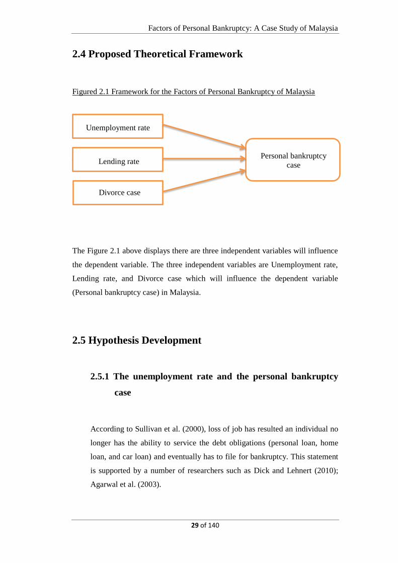
2.4 Proposed Theoretical Framework
Figured 2.1 Framework for the Factors of Personal Bankruptcy of Malaysia
xfnfnffngf
The Figure 2.1 above displays there are three independent variables will influence
the dependent variable. The three independent variables are Unemployment rate,
Lending rate, and Divorce case which will influence the dependent variable
(Personal bankruptcy case) in Malaysia.
2.5 Hypothesis Development
2.5.1 The unemployment rate and the personal bankruptcy
case
According to Sullivan et al. (2000), loss of job has resulted an individual no
longer has the ability to service the debt obligations (personal loan, home
loan, and car loan) and eventually has to file for bankruptcy. This statement
is supported by a number of researchers such as Dick and Lehnert (2010);
Agarwal et al. (2003).
Unemployment rate
Lending rate Personal bankruptcy
case
Divorce case

Factors of Personal Bankruptcy: A Case Study of Malaysia
30 of 140
H1a: The unemployment rate will positively influence the personal
bankruptcy case.
2.5.2 The lending rate and the personal bankruptcy case
According to Jappelli et al. (2008), changes in the nominal interest rate will
directly reflect on the lending rate offered by the banking and financial
institutions. Increases in nominal interest rate can increase the cost of
borrowers to service their debt level. As a result, for whose borrower who is
no longer has the ability to service the debt has no choice but to file for
bankruptcy. However, based on the finding of White (2010) states that the
climbing of insolvency rate is due to lower nominal interest rate. This has
increased the incentive of borrowing and resulted in higher insolvency rate.
H1b: The lending rate will positively influence the personal bankruptcy case.
2.5.3 Divorce case and the personal bankruptcy case
According to Zagorsky (2005) and Del Boca and Rocia (2001), the research
finding shows that divorce has lead to a reduction in household income,
followed by the expenses of alimony, legal fees, and children support fees
have eventually resulted in a bankruptcy filing. Besides, Fayet et al. (2002)
state that before a divorce, bankruptcy decision is often suggested by the
lawyers to discharge the debts owing by each other. This can ensure there
will be no lingering joint debt that the non-filing spouse will be responsible
for.
H1c: The divorce case will positively influence the personal bankruptcy case

Factors of Personal Bankruptcy: A Case Study of Malaysia
31 of 140
2.5.4 Long-run versus short-run
According to Hussain (2002), the author studies the macroeconomic
determinants (unemployment, interest rate, disposable income, and
household debt) of personal bankruptcy in the U.S. has found the existence
of a cointegration relationship in the model. Thus, in this study it is expected
the existence of a cointegration relationship in model.
H2: There is a cointegration relationship in the model.
2.5.5 Causal relationship
Granger causality test is being important because it can fill in the gap as
what the OLS cannot explain such as to explain the causal relationship. This
causal relationship can tell how the past values of Xt or Yt can use to predict
the future value of Yt or Xt respectively. The first objective of this test is to
examine the causal relationship between the independent variables/Xt
(unemployment rate, lending rate, and divorce case) towards the dependent
variable/Yt (Personal bankruptcy case). The second objective of this test is to
examine the causal relationship of the dependent variable/Yt towards the
independent variables/Xt (unemployment rate, lending rate, and divorce
case). The causal relationship can be categorized into a bidirectional,
unidirectional, and independent relationship. According to Jappelli et al.
(2008), the authors find a unidirectional relationship between the
unemployment rate and insolvencies as well as find an independent
relationship between interest rate and insolvencies both in the U.S and the
U.K. Nevertheless, there is a limited researcher using Granger causality to
investigate the causal relationship between all these variables. Therefore, the
actual causal relationship among these variables in this study is yet to
discover in Chapter 4 as the expected causal relationship among these
variables is hard to justify based on one single researcher only.

Factors of Personal Bankruptcy: A Case Study of Malaysia
32 of 140
H3a: Xt does Granger cause Yt
H3b: Yt does Granger cause Xt
2.6 Conclusion
Based on the literature review, it was found that the unemployment rate, the
lending rate, and divorce case have a significant effect on the personal bankruptcy
case. Based on the studies of different researchers, the unemployment rate and
divorce case are positively correlated on the personal bankruptcy case. On the
other hand, the lending rate has an ambiguous effect on the personal bankruptcy
due to different researcher has a different point of view and obtained different
findings. The methodology will be discussed further in the following chapter.

Factors of Personal Bankruptcy: A Case Study of Malaysia
33 of 140
CHAPTER 3: METHODOLOGY
3.1 Introduction
The methodology of the study will be discussed further in this chapter. Firstly,
discuss the data collection. Secondly, diagnostic checking will be carried out to
ensure the data are free from econometric error. Thirdly, regression analysis by
using OLS. Fourth, using Johansen cointegration test to examine the existence of a
cointegration relationship the model. Lastly, using Granger causality to examine
the causal relationship among the variables.
3.2 Data Collection Methods
Based on Sekaran (2005), data collection methods are a critical part of research
design. Data collection is a technique of collecting information and the
information collected can be applied for research purpose or in decision making
purpose. Basically, data can be categorized into primary and secondary data.
Primary data refers to the first hand data collected by the researcher to conduct
exploratory research. Secondary data, on the other hand, data is made accessible
to the public sources. In this research, secondary data has been collected from the
Department of Statistics Malaysia (DOSM). The sample sizes consist of 31 years
of annual data, covering from the year 1985 and 2015 both for dependent and
independent variable. The table 3.1 shows the sources and data explanation.

Factors of Personal Bankruptcy: A Case Study of Malaysia
34 of 140
Table 3.1: Sources and Data Explanation
Variables Units Explanation Sources
Personal
bankruptcy
Case reported Number of personal bankruptcy
case reported in Malaysia.
DOSM
Unemployment Percentage Unemployment rate in Malaysia DOSM
Lending Percentage Average lending rate offers by
the commercial bank in
Malaysia.
DOSM
Divorce Case reported Number of divorce case reported
in Malaysia.
DOSM
Notes: Department of Statistics of Malaysia (DOSM)
In this research, the software of E-Views 7 was used to analyze the data. Basically,
E-Views is an interactive econometric software which allows to conduct data
analysis, data estimation and, data forecasting. An empirical analysis of Ordinary
Least Squares (OLS) will be carried out by using E-views. By using this method,
econometric problems can be identified from the empirical model. Subsequently,
the solution to resolve the econometric problems will be given in order regressed
the model that is free from error.
3.3 Data Analysis
First of all, OLS test will be carried out to answer the Research Objective 1 to
identify the relationship between the personal bankruptcy case and the
unemployment rate, lending rate, and divorce case. Economic Model of the study
is as shown in below:
BANKRUPTCY= f(UNEMPLOYMENT, LENDING, DIVORCE)

Factors of Personal Bankruptcy: A Case Study of Malaysia
35 of 140
Thus, the Economic Model is constructed as:
LOGBANKRUPTCYt= β0 + β1UNEMPLOYMENTt + β2LENDINGt +
β3LOGDIVORCEt + 𝜀𝑡 rj
Where,
LOGBANKRUPTCY: Logarithms of personal bankruptcy case
UNEMPLOYMENT: Unemployment rate
LENDING: Lending rate
LOGDIVORCE: Logarithms of divorce case
3.3.1 Ordinary Least Squares (OLS)
Ordinary least squares (OLS) is one of the simplest of linear regression
model. It used to estimate the unknown parameters in a linear regression
model with a goal to minimizing the sum of squared errors from the data.
Graphically, if draw a regression line along a given data set, the closer
the distance of the corresponding points along the regression line, the
better the model fits the data. Generally, the OLS estimators are said to
be the best linear unbiased estimator only when the OLS has fulfilled all
the seven assumptions. These assumptions includes: 1) The OLS
estimator is a linear regression model, 2) Fixed X values, 3) there is a
zero mean value of disturbance, 4) the sample size must greater than the
number of parameters estimated, 5). There must be variation in the
values of the X variables, 6) No heteroscedasticity problem, and 7) No
autocorrelation problem (Gujarati and Porter, 2009).
In fact, the OLS is being a popular technique to use in the research field
due to it is easy to implement. In this research, the first and foremost test
to run is the unit root test to test for the stationary properties of the
(3.1)

Factors of Personal Bankruptcy: A Case Study of Malaysia
36 of 140
variables. Followed by diagnostic checking (multicollinearity,
heteroscedasticity, model specification, normality and, autocorrelation)
needed to carry out to ensure the econometric model is error free. Lastly,
Granger causality is applied to see whether the independent variables can
used to forecast the future dependent variable in Malaysia.
3.4 Diagnostic Checking
3.4.1 Unit Root Test
The unit root test is used to examine whether the stationary properties
exist in the time series variables. When the mean, variance, and
covariance are constant over time, this means that the series is stationary.
Oppositely, when the mean, variance, and covariance change over time
period, then it is consider as a non-stationary time series. The data will
tends to be forecasted with no biases if the data has stationary properties.
Unit root test uses negative value in the test. The negative number
meaning the possibility of rejecting the hypothesis where there is a unit
root at some level of confidence is greater. Besides, it is crucial to
identify the most appropriate form of trend in the data. Therefore, unit
root test always used in determining the appropriate form of whether
trending data should be first differenced or it should be regressed on
deterministic functions of time to ensure the stationary of the data. If
there are trending data in the model, then if should undergo detrending
process which is first differencing and time-trend regression. The I(1)
time series is more suitable for first differencing whereas the I(0) time
series is more suitable for the time-trend regression.
Under the null hypothesis, the initial Dickey Fuller (DF) unit root test
assumed that the differences in the series are serially uncorrelated.
Factors of Personal Bankruptcy: A Case Study of Malaysia
37 of 140
However, when the time series undergoes first differences, this means
that the time series will become serially correlated. In other words, this
indicates the DF has been transformed into ADF test. The transformation
of the model removes the serial correlation in the error term of the model.
3.4.1.1Augmented Dickey Fuller Test (ADF)
Augmented Dickey-Fuller (ADF) is a test which further developed
by Dickey and Fuller (1981) due to autocorrelation problem exist in
DF test. This is the first approach that used to test for the
stationarity of time series data with the condition of large sample
size. The equation is as shown in below:
∆𝑌𝑡 = 𝛼𝑌𝑡−1 + 𝛽1∆𝑌𝑡−1 + 𝛽2∆𝑌𝑡−2 + ⋯ + 𝛽𝑝∆𝑌𝑡−𝑝 + 𝑉𝑡 (3.2)
Assume that the dependent variable follows an AR(p) process, the
number of the lagged differenced terms of dependent variable will
be included in the equation. The changes of dependent variable
which consisted of constant and total lagged of changes in
dependent variables, and white noise change, Vt. The null and
alternative hypothesis for unit root test is:
𝐻0: The variables are non-stationary (unit root)
𝐻1: The variables are stationary (no unit root)
The null hypothesis has a unit root, means non-stationary with
integrated order I(1), while alternative hypothesis has no unit root,
means stationary with integrate order I(0). In this paper, the results
obtained will be considered as dynamic stationary at I(1). In order to
obtain I(1) in the level form, the p-value must be larger than alpha at

Factors of Personal Bankruptcy: A Case Study of Malaysia
38 of 140
1% and 5% such that do not reject null hypothesis. Subsequently,
through the first difference form to become stationary where the p-
value is smaller than alpha at 1%, 5% and 10%, such that reject null
hypothesis (Gujarati and Porter, 2009).
3.4.1.2 Philips-Perron Test (PP)
Philips-Perron test (PP) is also one of the tests for unit root.
According to Gujarti and Porter (2009), PP is using the non-
parametric method to take on the serial correlation in the error terms
that lacking addition of lagged difference terms. PP test is similar
with the ADF test, the mainly difference between these two tests is
the way they handle the serial correlation in the regression. For
ADF test, its ARMA structure of the errors in the test regression
used a parametric autoregression to estimate error term, but the PP
tests just fail to consider any serial correlation in the test regression.
The hypothesis of PP can be written as:
𝐻0: The variables are non-stationary (unit root)
𝐻1: The variables are stationary (no unit root)
The decision rule for PP test is identical as ADF test where the H0
will be rejected only when the p-value is smaller than 1% or 5%
significance level. Otherwise, do not reject H0.
Factors of Personal Bankruptcy: A Case Study of Malaysia
39 of 140
3.4.2 Normality Test
H0: The sample data are normally distributed
H1: The sample data are not normally distributed
Normality test for the sample data is playing a critical role in the OLS
model (Gujarati and Porter, 2009). When the properties of the sample
data are normally distributed, this signifies the estimated result is
consistent, unbiased and efficient estimator, and otherwise the result is
not reliable. In this research, Jarque-Bera test has been applied to test the
normality properties of the sample data. In order to ensure the model is
free from the econometric problems, thus, must ensure the p-value
obtained is larger than 5% significance level. Otherwise, the model has
normality problem.
3.4.3 Multicollinearity Test
Multicollinearity problem will only occur in multiple regression models
in which the independent variables are highly correlated with one
another. In this case, the regression model is difficult to explain which
independent variables are actually affecting the dependent variable (Paul,
2006). There are some practical consequences of multicollinearity
which are large variance and covariances of OLS estimators,
“Insignificant” t ratio and, wider confidence intervals. In fact, there is no
one unique method to detect multicollinearity or measuring it is strength,
but there is some rule of thumb to detect it. Firstly, high R-squared but
few significant t ratios can be detected from the OLS output generated
by E-Views. Secondly, High pair-wise correlation coefficients can use to

Factors of Personal Bankruptcy: A Case Study of Malaysia
40 of 140
detect multicollinearity when the coefficient is closed to 1 (specifically is
more than 0.8).
Lastly, Variance Inflation Factor (VIF) also can be used to detect
multicollinearity in a regression model. If the VIF is >10, this signifies
that the independent variables are highly correlated in the model
(Gujarati and Porter, 2009). There some remedial to counter the
multicollinearity problem such as dropping a variable and increase the
sample size.
3.4.4 Heteroscedasticity
H0: Homoscedasticity among the error terms
H1: Heteroscedasticity among the error terms
One of the assumptions of OLS estimator is the error terms must be in
heteroscedasticity. This means the error terms must not correlate with
each other as well as they have the same variance across the sample size.
Otherwise, if heteroscedasticity occurs, the OLS estimators for the
coefficients are still unbiased and consistent. However, the estimators of
the OLS method will become inefficient due to the increasing in the
variances of the distribution (Hayes and Cai, 2007). In short, this will
lead to hypothesis testing invalid and make the wrong conclusion. There
are a numbers of methods to detect heteroscedasticity problems such as
Park test, Glesjer test, Breusch-Pagam-Godfrey test, Whites’ test and
Autoregressive Conditional Heteroscedasticity (ARCH) test.

Factors of Personal Bankruptcy: A Case Study of Malaysia
41 of 140
In this research, ARCH test has been applied to detect heteroscedasticity
problem in the model. ARCH test has been selected among other
detection methods because ARCH test is the only test applicable for time
series data. Based on the hypothesis testing, null hypothesis means
homoscedasticity and other wise. Thus, must ensure the p-value is
greater than the significance level of 5%, subsequently, there is
insufficient evidence to reject null hypothesis given null hypothesis is
true. This signifies the error term is homoscedasticity and with the same
variance across the sample size. White’s Heteroscedasticity-Corrected
Variances and Standard Error method can be used to counter the
heteroscedasticity problem if this problem is exists in the model.
3.4.5 Model Specification
H0: There is correctly specified
H1: There is not correctly specified
Model specification is another important diagnostic checking of data
analysis. The model is said to have specification bias due to a few factors.
Firstly, omitting a relevant independent variable which could play an
important role to affect the dependent variable. Secondly, including an
irrelevant independent variable in the model and lead to the estimated
coefficient to become biased and inconsistent. Lastly, adopting the
wrong functional form of dependent and independent variable (Gujarati,
2012). Model specification bias can be detected by using Ramsey
Regression Equation Specification Error Test (RESET) test. The null
hypothesis is there is no specification biasl. Therefore, must make sure
the p-value is greater than the significant level of 5%. This signifies the
model is free from specification bias and other wise.

Factors of Personal Bankruptcy: A Case Study of Malaysia
42 of 140
3.4.6 Autocorrelation
H0: The error terms are not correlated over time
H1: The error terms are correlated over time
Autocorrelation problem is the error terms for any observation are
related to the error terms of other observation. One of the reason lead to
this problem can be due to the omission of relevant independent
variable or misspecification of true error term (Babatunde, Ikughur,
Ogunmola, Oguntunde, 2014). There are a number of consequences of
autocorrelation on the OLS estimators. Firstly, the OLS estimators are
still unbiased and consistent. This is because both unbiasedness and
consistency have nothing to do on with the assumption of no
autocorrelation of the error term.
Secondly, the OLS estimators is no longer efficient and thus, no longer
the Best, Linear, Unbiased, Estimator (BLUE). This is because the
serially correlated error term will lead to the dependent variable to
fluctuate in a way that the OLS estimation procedure sometimes
attributes to the independent variables. Consequently, the OLS has
higher chance to overestimate or under estimate the true coefficient.
Lastly, the estimated variances of the regression coefficients will be
biased and inconsistent and, resulted hypothesis testing invalid. There
are three methods to detect autocorrelation which are Durbin-Watson
test, Durbin’s h test, and Breusch-Godfrey LM test. In this research,
Breusch-Godfrey LM test has been applied to detect the autocorrelation
problem. This is because LM test is applicable to detect in time series
data regardless the model has autoregressive or not. Since the null
hypothesis is there is no autocorrelation problem and therefore, it is
important to obtain a p-value that is greater than the significant level of

Factors of Personal Bankruptcy: A Case Study of Malaysia
43 of 140
5%. This signifies the error terms are not correlated overtime. In other
words, no autocorrelation in the model.
However, in the case of having autocorrelation problem in the mdoel,
first is try to find out if the autocorrelation is pure autocorrelation and
not due to mis-specification. If it is pure auto correlation, Cochrane -
Orcutt procedures can be applied to counter the problem. In the case of
large samples, on the other hand, Newey – West method can be applied
to obtain standard errors of OLS estimators that are corrected for
autocorrelation.
3.5 Inferential Statistics
3.5.1 R-Squared
R-Square statistics is often emphasizing in the regression analysis, it
provides a single number in telling how well the regression model fits
the data. If the R-Squared value equal to 1 means that 100 percent of the
variation observed in the dependent variable is captured by the
independent variables in the regression model. This means the
regression model perfectly fits the data. On the contrary, if the R-
Squared value is 0.01, this shows that the regression model only can
capture percent of the observed variation in the data. In other words,
there are 99 percent of the observed variation in the dependent variable
is not explained by the model used in the regression. As mentioned in
(Gujarati and Porter, 2009), the cross-sectional analysis will normally
obtain a lower R-Squared whereby in time series analysis tends to
obtain a higher R-Squared. However, the R-Square value how “high”
only consider as high is still remain an argumentative topic for most of
the researcher, yet a majority of the researcher agreed that as long as the

Factors of Personal Bankruptcy: A Case Study of Malaysia
44 of 140
R-Squared value is above 50 percent can consider as high R-Squared
(Gujarati and Porter, 2009; Reisinger, 1997). There is a major limitation
of R-Squared that make it less preferable to be interpreted in the result.
This is because the R-Squared value can be increased by adding the
number of independent variables regardless of how well the
independent variables are correlated with the dependent variable. As an
alternative, adjusted R-Squared is used in explaining the fitness of the
data on the regression model.
3.5.2 Adjusted R-Squared
The adjusted R-Squared is having the similar concept as the R-Squared
but, is has been adjusted for the number of predictors in the model. This
means that the adjusted R-Squared value will be increased only when
the independent variable has a correlation with the dependent variable.
Conversely, any independent variable without a strong correlation will
result in a lower adjusted R-Squared value. The adjusted R-squared
value and the R-squared value will be equal only when there is only one
independent variable, however, by adding the number of independent
variable the adjusted R-squared value will keep dropping (Gujarati and
Porter, 2009).
3.5.3 F-test Statistic
H0: There is no difference between the variances
H1: There is at least 1 difference between the variances
Factors of Personal Bankruptcy: A Case Study of Malaysia
45 of 140
F-test is a statistical test used to determine the overall significance of the
regression model. It is commonly applied to test whether the model is
best fits the population based on the sample data set. This means that F-
test is to examine whether there is at least a minimum of 1 independent
variable can significantly to explain the dependent variable. The null
hypothesis is all the coefficients of the independent variables are equal to
zero or there is no difference between the variances. The alternative
hypothesis, on the other hand, is at least one difference between the
variances. Reject the null hypothesis if the p-value is smaller than 5%
significance level. This signifies there is at least one difference between
the variances.
3.5.4 T-test Statistic
H0 = β1 = 0, β2 = 0, β3 = 0 (Insignificant)
H1 = β1≠0, β2≠0, β3≠0 (Significant)
Where,
β1 = Unemployment rate
β2 = Lending rate
β3 = Logarithms of divorce case
T- test statistics is used to determine the relationship as well as the
significance level between an independent and dependent variable
(Gujarati and Porter, 2009). Besides that, this test also allows to
examine whether the means of the two samples are statistically different
from each other. According to Park (2009), there is a key assumption of
T-test where the samples are randomly chosen from normally
distributed populations without any selection bias. The null hypothesis
is the individual regression coefficients are equal to zero. The

Factors of Personal Bankruptcy: A Case Study of Malaysia
46 of 140
alternative hypothesis, on the other hand, the coefficients are not equal
to zero. Reject the null hypothesis of the p-value is smaller than 5%
significance level. This signifies the independent variable and the
dependent variable has a significant relationship.
3.6 Johansen Co-integration Test
Johansen cointegration test is employed to answer the Research Objective 2 by
examining the existence of cointegration relationships in the model. The test often
suggests that cointegrated time series variables cannot shift too far away from
each other and the cointegrations of these variables are stationary although
individually they aren’t. Johansen’s methodology takes vector autoregressive
(VAR) models as its starting point and giving permission the testing of hypothesis
as regards the equilibrium relationship between the variables (Gujarati, 2009).
Besides, the spurious rejection rate can be minimized by using the cointegration
test. Moreover, the stated frequency persists in being immense and seems to build
up with the quantity of the selected variables in the system, despite applying a
number of specification tests (Osterholm and Hjalmarsson, 2007).
In fact, under the comparison between the different types of cointegration test,
Johansen’s approaches are more sensible property than Engle and Granger.
Researchers would prefer to apply the results of Johansen-Juselius on the
asymptotic distribution of the likelihood ratio test as the asymptotic distribution of
involves an integral of a multivariate Brownian motion with respect to itself. The
Engle-Grangers Two Step Estimation method is easier to run but it can be only
run on a maximum of two variables and as opposed to Johansen’s method, it
doesn’t allow for hypothesis testing on cointegrating relationships (Gujarati, 2012).
Furthermore, Gujarati (2012) concludes that Johansen’s approach is far more
superior compared to others even under circumstances where errors not being

Factors of Personal Bankruptcy: A Case Study of Malaysia
47 of 140
normally distributed, or the dynamics of the vector error-correction model
(VECM) are uncertain and an inclusion of additional lags in the VECM.
3.7 Vector Error Correction Model (VECM)
VECM is a multivariate generalization of error correction model derived from the
VAR model to analyze non-stationary time series data. The specification of
VECM comprises the cointegration relation and explains how the examined model
coincides to the long-run relationships while also enabling the short-run
adjustment dynamics.
The estimation accessible approaches can be different for the estimation of a
model of type (1) based on the exact model specification. Providing that no zero
restrictions on the matrices as well as lacking of exogenous variables, making it a
reduced form model is specified without presence of exogenous variables and
given that each equation has the identical right-hand side variables, then the
Johansen reduced rank (RR) estimation procedure (Johansen, 1988) and simple
two step (S2S) method was started by Lutkepohl and Kratzig (2005) can be
applied.
The general form of vector error correction model (VECM) can be characterized
as below:
Δ𝐵𝑎𝑛𝑘𝑡 = 𝛽0 + ∑ 𝛽1𝑛𝑖 Δ𝐵𝑎𝑛𝑘𝑡−𝑖 + ∑ 𝛽2
𝑛𝑖 Δ𝑈𝑛𝑒𝑚𝑝𝑡−𝑖 + ∑ 𝛽3
𝑛𝑖 Δ𝐿𝑒𝑛𝑑𝑡−𝑖 +
∑ 𝛽4𝑛𝑖 Δ𝐷𝑖𝑣𝑜𝑡−𝑖 + 𝜇𝑖𝐸𝐶𝑇𝑡−1 + Ɛ1,𝑡 (3.3)

Factors of Personal Bankruptcy: A Case Study of Malaysia
48 of 140
Δ𝑈𝑛𝑒𝑚𝑝𝑡 = 𝛽0 + ∑ 𝛽1𝑛𝑖 Δ𝑈𝑛𝑒𝑚𝑝𝑡−𝑖 + ∑ 𝛽2
𝑛𝑖 Δ𝐵𝑎𝑛𝑘𝑡−𝑖 + ∑ 𝛽3
𝑛𝑖 Δ𝐿𝑒𝑛𝑑𝑡−𝑖 +
∑ 𝛽4𝑛𝑖 Δ𝐷𝑖𝑣𝑜𝑡−𝑖 + 𝜇𝑖𝐸𝐶𝑇𝑡−1 + Ɛ2,𝑡 (3.4)
Δ𝐿𝑒𝑛𝑑𝑡 = 𝛽0 + ∑ 𝛽1𝑛𝑖 Δ𝐿𝑒𝑛𝑑𝑡−𝑖 + ∑ 𝛽2
𝑛𝑖 Δ𝐵𝑎𝑛𝑘𝑡−𝑖 + ∑ 𝛽3
𝑛𝑖 Δ𝑈𝑛𝑒𝑚𝑝𝑡−𝑖 +
∑ 𝛽4𝑛𝑖 Δ𝐷𝑖𝑣𝑜𝑡−𝑖 + 𝜇𝑖𝐸𝐶𝑇𝑡−1 + Ɛ3,𝑡 (3.5)
Δ𝐷𝑖𝑣𝑜𝑡 = 𝛽0 + ∑ 𝛽1𝑛𝑖 Δ𝐷𝑖𝑣𝑜𝑡−𝑖 + ∑ 𝛽2
𝑛𝑖 Δ𝐵𝑎𝑛𝑘𝑡−𝑖 + ∑ 𝛽3
𝑛𝑖 Δ𝑈𝑛𝑒𝑚𝑝𝑡−𝑖 +
∑ 𝛽4𝑛𝑖 Δ𝐿𝑒𝑛𝑑𝑡−𝑖 + 𝜇𝑖𝐸𝐶𝑇𝑡−1 + Ɛ4,𝑡 (3.6)
Where,
Bank = Logarithms of personal bankruptcy case
Unemp = Unemployment rate
Lend = Lending rate
Divo = Logarithms of divorce case
ECTt-1 = Yt-1 - 𝛽1 - 𝛽2Xt-1
Ɛt = Residual
µi = Error correction coefficient
3.8 Granger Causality Test
Lastly, Granger causality is used to determine whether the time series variables
are useful for the prediction of another time series variable. This test is use to
answer the Research Objective 3. Granger (1969) stated that the Granger causality
test is defined as the correlation between the present value of a variable and the
past value of a different variable. This test defined as variable Yt is said to
Granger-cause Xt, if Xt can be better predicted using the histories of both variables
Xt and Yt rather than using past values of variable Xt alone, all of the other terms
remain constant. Since, the future is unable to the predict past, when variable Xt

Factors of Personal Bankruptcy: A Case Study of Malaysia
49 of 140
Granger causes variable Yt, then changes in Xt should precede changes in Yt. The
concept of Granger causality test is analysed with predictability approaches and
taking advantage of the direction of the time flow to attain a causal ordering of
related variables. Considering it does not depend on the specification of an
econometric model, it is acceptable for empirical model building strategies. There
are three possible types of Granger causality.
H0 = Xt does not Granger cause Yt
H1 = Xt does Granger cause Yt
H0 = Yt does not Granger cause Xt
H1 = Yt does Granger cause Xt
The first type is both of the null hypotheses are not rejected, two series variable is
independent. For the second type, the series will have bidirectional casual effect if
both null hypotheses testing is rejected. Lastly, if there is only one of the null
hypotheses testing rejected, there will be a unidirectional causal effect (Granger,
1969). Foresti (2006) stated that Granger causality test can be applied when there
are three different situations. For the first one, there are two variables with their
respective lags in the basic Granger causality test. Later on, there are not only two
variables and their lags in the Granger causality test.
3.9 Impulse Response Function
The impulse response function (IRF) is a complimentary test use together with the
granger causality test. This is because the Granger causality test has its own
limitation in telling the Granger cause in the short run is positively cause or
negatively cause, how long the effects will last for, as well as it does not provide
evidence of this effect is direct or indirect cause. By using IRF, on the other hand,

Factors of Personal Bankruptcy: A Case Study of Malaysia
50 of 140
all the limitations of the Granger causality test can be overcome and thus, IRF is
also tested in this research.
According to Gujarati (2009), IRF can be used to identify the responsiveness of
the dependent variables in both unrestricted VAR and VECM towards the
macroeconomic shocks. The results of the IRF will be reliable only when the time
series data achieved stationary after passing through the second difference form.
Furthermore, it also performs like an economic function to identify what will be
the likely impact caused on all the variables in the VECM when there is a shock
occurs. Additionally, IRF also can detect the response of any variable towards the
all other variables in the system (Gujarati, 2009). The ordering of the variables is
playing an important role in the IRF this is because it can directly affect the result
reported even though the same set of data is using.
3.10 Conclusion
In this research is using time series data where the investigation period is from the
year 1985 and 2015 and the frequency is in annually. In the total of 31 sample size
are taken from each independent variables (Unemployment rate, Lending rate, and
Divorce case reported), and the dependent variable (Personal bankruptcy case
reported) for this study. All the data is collected from DOSM and processed by
using E-Views 7. In this research, diagnostic checking has been to ensure all the
variables are free from econometric problem. Subsequently, Johansen
cointegration is applied to test for the existence of the long-run relationship
between the variables. The existence of the long run relationship allows to apply
VEC model is applied to test for the speed of adjustment toward the long run
equilibrium. Lastly, the empirical results will be discussed further in the next
chapter.

Factors of Personal Bankruptcy: A Case Study of Malaysia
51 of 140
CHAPTER 4: DATA ANALYSIS
4.1 Introduction
The data analysis in this chapter will present the interpretation as well as analyse
the empirical findings from the methodology in order to answer the Research
Objectives.
4.2 Diagnostic Checking
4.2.1 Unit root Test
The first and foremost test to begin with is the examination of the
stationary properties of the variables, which are the personal bankruptcy
case, the unemployment rate, lending rate, and divorce case by using unit
root test. In this research, ADF and PP test were used to determine the
stationary properties of the variables. The null hypothesis for both ADP
and PP states that the variables have a unit root, means the variables is
non-stationary.
Based on Table 4.1, the variables are tested both at the level form and
first difference form with the inclusion of intercept without trend and
intercept with a trend. The optimal number of lag length in ADF test is
determined based on Schwarz Info Criterion (SIC), while the optimal lag
length in PP test is determined based on Newey-West Bandwidth. The
results of ADF show that the test statistics for the personal bankruptcy

Factors of Personal Bankruptcy: A Case Study of Malaysia
52 of 140
case, the unemployment rate, lending rate, and divorce case are greater
than the critical values at 1%. In other words, there is a statistically
insignificant to reject null hypothesis at the level form. On the other hand,
the results of PP test show that the test statistics for the four variables are
also statistically insignificant to reject the null hypothesis at the level
form as well. In short, ADF and PP tests have provided a conclusion for
the personal bankruptcy case, unemployment rate, lending rate, and
divorce case are non-stationary at the level form.
Next, the first difference in ADF is concluded for the four variables. The
results show that the null hypothesis of non-stationary is being rejected
at 1% significance level for all the four variables. Meanwhile, the result
from PP test also reveals that the test statistics for the four variables are
statistically significant to reject the null hypothesis at 1% significance
level. Thus. This can conclude that the personal bankruptcy case,
unemployment rate, lending rate, and divorce case are stationary at first
difference.
Table 4.1: The results of unit root tests
Level
Without Trend With Trend
Variables ADF PP ADF PP
BANKRUPTCY 0.0855 0.0316 0.0174 0.1271
UNEMPLOYMENT 0.4375 0.4255 0.0433 0.8567
LENDING 0.7439 0.8501 0.3496 0.3838
DIVORCE 0.9867 0.9823 0.1943 0.4703
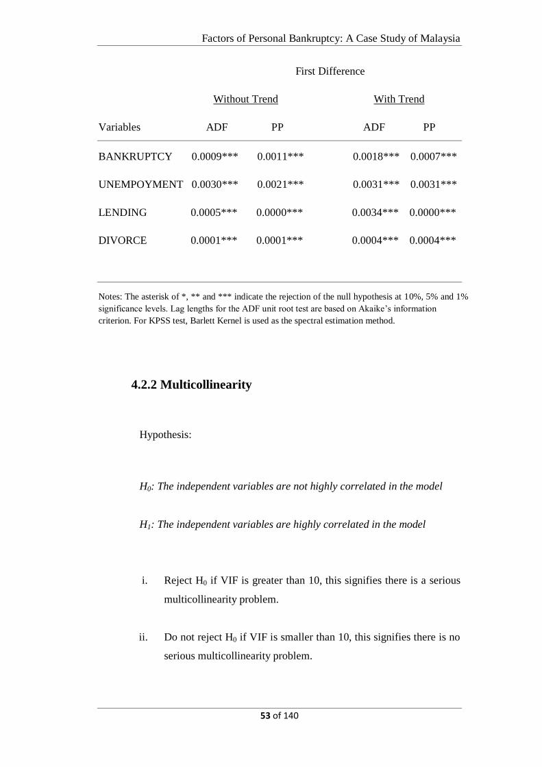
Factors of Personal Bankruptcy: A Case Study of Malaysia
53 of 140
First Difference
Without Trend With Trend
Variables ADF PP ADF PP
BANKRUPTCY 0.0009*** 0.0011*** 0.0018*** 0.0007***
UNEMPOYMENT 0.0030*** 0.0021*** 0.0031*** 0.0031***
LENDING 0.0005*** 0.0000*** 0.0034*** 0.0000***
DIVORCE 0.0001*** 0.0001*** 0.0004*** 0.0004***
Notes: The asterisk of *, ** and *** indicate the rejection of the null hypothesis at 10%, 5% and 1%
significance levels. Lag lengths for the ADF unit root test are based on Akaike’s information
criterion. For KPSS test, Barlett Kernel is used as the spectral estimation method.
4.2.2 Multicollinearity
Hypothesis:
H0: The independent variables are not highly correlated in the model
H1: The independent variables are highly correlated in the model
i. Reject H0 if VIF is greater than 10, this signifies there is a serious
multicollinearity problem.
ii. Do not reject H0 if VIF is smaller than 10, this signifies there is no
serious multicollinearity problem.

Factors of Personal Bankruptcy: A Case Study of Malaysia
54 of 140
Table 4.2: Pair-wise Correlation Analysis
LOGDIVORCE LENDING UNEMPLOYMENT
LOGDIVORCE 1.000000 0.875662 -0.557647
LENDING 0.875662 1.000000 -0.550533
UNEMPLOYMENT -0.557647 -0.557647 1.000000
*Results obtained from Eviews7
Based on the Table 4.2, there is a high correlation between the lending
rate (LENDING) and divorce case (DIVORCE). This is proven by the
high value of pair-wise correlation coefficient which is 0.875662. Based
on Gujarati and Porter (2009), if the pair-wise correlation coefficient is
greater than 0.8 that means there is a greater chance of the existing of
multicollinearity problem. Therefore, the correlation results of 0.875662
which is greater than 0.8 shows there is a higher chance of the existing of
the multicollinearity problem between the lending rate and divorce case.
In this case, may proceed to employ the Variance Inflation Factor (VIF)
to detect the multicollinearity problem. This study estimated the R2 by
transforming the independent variable into dependent variable to
compute the VIF, where VIF = 1
(1−R2xi,xj)
Table 4.3: Correlation Analysis
Dependent
variable
Independent
variable
R-squared VIF
LENDING DIVORCE 0.766785 1.000000

Factors of Personal Bankruptcy: A Case Study of Malaysia
55 of 140
Conclusion:
Based on Table 4.3, it shows that the VIF is falling between 1 and 10.
Therefore, the decision making is do not reject H0. This study can
conclude that the model does not have a serious multicollinearity
problem since the VIF of the independent variables are less than 10.
4.2.3 Heteroscedasticity
Hypothesis:
H0: Homoscedasticity among the error terms
H1: Heteroscedasticity among the error terms
Decision rules:
i. Reject H0 if the p-value is smaller than significant level at 5%.
This signifies there is a heteroscedasticity problem.
ii. Do not reject H0 if the p-value is greater than significant level
at 5%. This signifies homoscedasticity among the error term.
Table 4.4: Heteroscedasticity Test: ARCH
Obs*R-squared 2.931187 Prob. Chi-Square(1) 0.0869
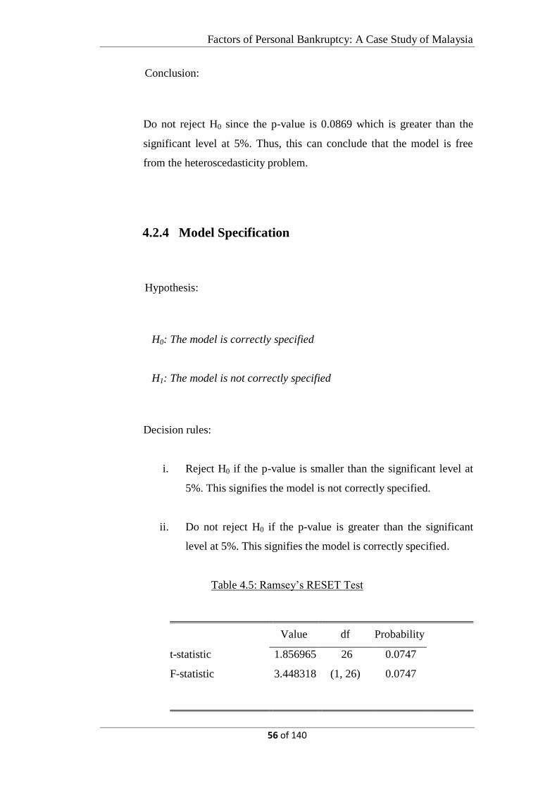
Factors of Personal Bankruptcy: A Case Study of Malaysia
56 of 140
Conclusion:
Do not reject H0 since the p-value is 0.0869 which is greater than the
significant level at 5%. Thus, this can conclude that the model is free
from the heteroscedasticity problem.
4.2.4 Model Specification
Hypothesis:
H0: The model is correctly specified
H1: The model is not correctly specified
Decision rules:
i. Reject H0 if the p-value is smaller than the significant level at
5%. This signifies the model is not correctly specified.
ii. Do not reject H0 if the p-value is greater than the significant
level at 5%. This signifies the model is correctly specified.
Table 4.5: Ramsey’s RESET Test
Value df Probability
t-statistic 1.856965 26 0.0747
F-statistic 3.448318 (1, 26) 0.0747
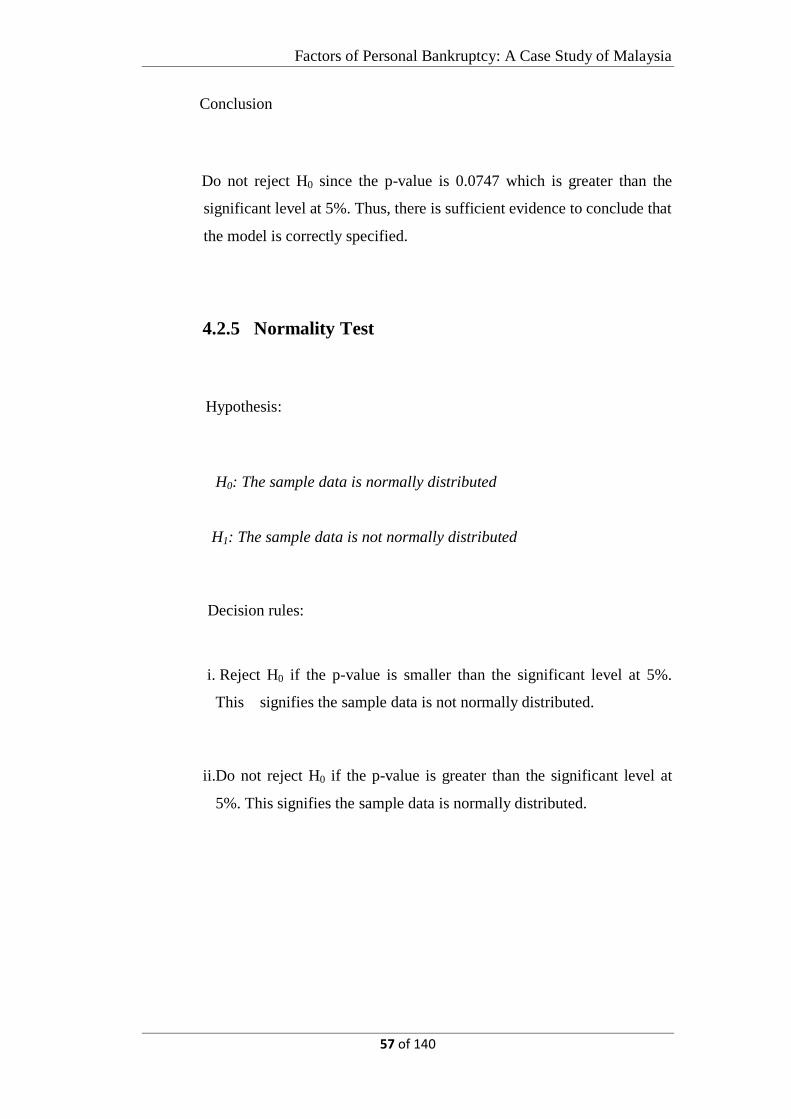
Factors of Personal Bankruptcy: A Case Study of Malaysia
57 of 140
Conclusion
Do not reject H0 since the p-value is 0.0747 which is greater than the
significant level at 5%. Thus, there is sufficient evidence to conclude that
the model is correctly specified.
4.2.5 Normality Test
Hypothesis:
H0: The sample data is normally distributed
H1: The sample data is not normally distributed
Decision rules:
i. Reject H0 if the p-value is smaller than the significant level at 5%.
This signifies the sample data is not normally distributed.
ii.Do not reject H0 if the p-value is greater than the significant level at
5%. This signifies the sample data is normally distributed.

Factors of Personal Bankruptcy: A Case Study of Malaysia
58 of 140
Table 4.6: Jarque-Bera Normality Test
Jarque-Bera 1.4354440 Probability 0.487863
Conclusion:
Do not reject H0 since the p-value (JB statistics) is 0.487863 which is
greater than the significant level at 5%. Thus, this can conclude that the
sample data is normally distributed in the model.
4.2.6 Autocorrelation
Hypothesis:
H0: The error terms are not correlated over time
H1: The error terms are correlated over time
Decision rules:
i. Reject H0 if the p-value is smaller than the significant level at
5%. This signifies the error terms are correlated over times or
the model has autocorrelation problem.
ii. Do not reject H0 if the p-value is greater than the significant
level at 5%. This signifies the error terms are not correlated
over time or the model is free from autocorrelation problem.

Factors of Personal Bankruptcy: A Case Study of Malaysia
59 of 140
Table 4.7: Breusch-Godfrey Seial Correlation LM Test
Obs*R-squared 9.843314 Prob. Chi-Square(2) 0.0073
Conclusion:
Reject H0 since the p-value (Chi-Square) is 0.0073 which is smaller than
the significant level at 5%. Thus, there is sufficient evidence to conclude
that there is autocorrelation problem in the model. In this case, Newey-
West HAC Standard Errors will be used to overcome the autocorrelation
problem.
4.3 Multiple Linear Regression Model
This study employed OLS method to form a Multiple Linear Regression Model in
order to study the relationship of the personal bankruptcy (BANKRUPTCY) in
Malaysia with the determinants of the unemployment (UNEMPLOYMENT
RATE), lending (LENDING RATE) and, divorce case (DIVORCE). Below is the
estimated Economic Model:
𝐋𝐎𝐆𝐁𝐀𝐍𝐊𝐑𝐔𝐏𝐓𝐂𝐘 = ̂ �̂�0 + �̂�1UNEMPLOYMENT + �̂�2LENDING +
�̂�3LOGDIVORCE
(4.1)

Factors of Personal Bankruptcy: A Case Study of Malaysia
60 of 140
Therefore, the results were estimated as shown in Table 4.8.
Table 4.8: Regression Results for OLS model
Dependent variable:
Bankruptcy
Independent variables Constant Unemployment Lending Divorce
Coefficient 4.7159 -0.1219 0.0759 0.4422
t-Statistic 4.7423 -2.7343** 3.3212*** 4.5102***
p-value 0.0001 0.0109 0.0026 0.0001
R2
0.8750
�̅�2 0.8611
F-statistic 63.0066
Prob(F-statistic) 0.0000***
Observation 31
Notes: The reported results are adjusted for autocorrelation problem by using Newey-West method.
:*, ** and *** represent the null hypothesis will be rejected at 10%, 5% and 1%
significance level respectively.
4.3.1 Interpretation on Intercept Coefficient and
Independent Variables
Based on the regression result, each of the independent variable is
interpreted as below:
�̂�0 = 4.7159. The coefficient of the intercept is 4.7159.The estimated
personal bankruptcy case in Malaysia is 4.7159 percent that could not be
explained by the independent variables of the unemployment rate,
lending rate, and divorce case.
�̂�1 = -0.1219. The t-statistics for the unemployment is -2.7344, which is
significant at 5 percent significance level. The coefficient result of the
unemployment rate is -0.1219, the negative sign indicates there is a

Factors of Personal Bankruptcy: A Case Study of Malaysia
61 of 140
negative relationship between the unemployment rate and the personal
bankruptcy case in Malaysia. The coefficient also means that holding
other variables constant, if the unemployment rate increases by 1 percent,
on average, the estimated personal bankruptcy case in Malaysia will
decrease by 12.19 percentage point, ceteris paribus assumption.
�̂�2 = 0.0759. The t-statistics for the lending rate is 3.3212, which is
significant at 1 percent level. The coefficient result of the lending rate is
0.0759, the positive sign indicates there is a positive relationship
between the lending rate and the personal bankruptcy case in Malaysia.
The coefficient also means that holding other variables constant, if the
lending rate increases by 1 percent, on average, the estimated personal
bankruptcy case in Malaysia will increase by 7.5986 percent point,
ceteris paribus assumption.
�̂� 3 = 0.4422. The t-statistics for divorce case is 4.5102, which is
significant at 1 percent level. The coefficient is 0.4422, the positive sign
indicates there is a positive relationship between the divorce case and the
personal bankruptcy case in Malaysia. The coefficient also means that
holding other variables constant, if the divorce case increases by 1
percentage point, on average, the estimated personal bankruptcy case in
Malaysia will increase by 44.22 percentage point, ceteris paribus
assumption.

Factors of Personal Bankruptcy: A Case Study of Malaysia
62 of 140
4.4 Inferential Analyses
4.4.1 Interpretation on R2 and �̅�2
Based on the R2, there is approximately 87.50% of the variation in the
personal bankruptcy case could be explained by the variation in
independent variables which are the unemployment rate, lending rate and,
divorce case. Meanwhile, from the �̅�2, there is approximately 86.11% of
the variation in the personal bankruptcy case could be explained by the
variation in independent variables which are the unemployment rate,
lending rate and, divorce case after taking the degree of freedom into
account.
4.4.2 F-test Statistic
F-test is employed to test the overall difference in the variances of the
economic model.
Hypothesis:
H0: There is no difference between the variances
H1: There is at least 1 difference between the variances

Factors of Personal Bankruptcy: A Case Study of Malaysia
63 of 140
Decision rules:
i. Reject H0 if the p-value (F-Statistic) is smaller than the
significant level at 1%. This signifies there is at least 1
difference between the variances or there is minimum of 1
independent variable
ii. Do not reject H0 if the p-value (F-Statistic) is greater than
the significant level at 5%. This signifies there is no
difference between the variances or all the independent
variable are significantly to explain the dependent variable.
Conclusion:
Based on Table 4.8: The result shows do not reject H0 since the p-value
is significant at 1% significance level. This can conclude that there is at
least 1 difference between the variances.
4.4.3 T-test Statistic
In this study, T-test is employed to test the relationship between
individual partial regression coefficient and dependent variable.

Factors of Personal Bankruptcy: A Case Study of Malaysia
64 of 140
4.4.3.1 Unemployment rate
Hypothesis:
H0: Unemployment rate does not have significant a
relationship with personal bankruptcy case.
H1a: Unemployment rate have a significant relationship with
the personal bankruptcy case.
Decision Rules:
i. Reject H0 if the p-value (t-statistic) is smaller than
the significant level at 5%. This signifies there is
significant relationship between the two variables.
ii. Do not reject H0 if the p-value is greater than the
significant level at 5%. This signifies there is no
significant relationship between the two variables.
Conclusion:
By referring to Table 4.8: Regression results: reject H0 since the p-
value is 0.0109 which is significant at 5%.

Factors of Personal Bankruptcy: A Case Study of Malaysia
65 of 140
4.4.3.2 Lending rate
Hypothesis:
H0: Lending rate does not have a significant
relationship with the personal bankruptcy case.
H1b: Lending rate have a significant relationship with the
personal bankruptcy case.
Decision Rules:
i. Reject H0 if the p-value (t-statistic) is smaller than
the significant level at 5%. This signifies there is
significant relationship between the two variables.
ii. Do not reject H0 if the p-value is greater than the
significant level at 5%. This signifies there is no
significant relationship between the two variables.
Conclusion:
By referring to Table 4.8: Regression results: reject H0 since the p-
value is 0.0026 which is significant at 1%.

Factors of Personal Bankruptcy: A Case Study of Malaysia
66 of 140
4.4.3.3 Divorce case
Hypothesis:
H0: The divorce case does not have a significant
relationship with the personal bankruptcy.
H1c: The divorce case have a significant relationship with
the personal bankruptcy.
Decision Rules:
i. Reject H0 if the p-value (t-statistic) is smaller than
the significant level at 5%. This signifies there is
significant relationship between the two variables.
ii. Do not reject H0 if the p-value is greater than the
significant level at 5%. This signifies there is no
significant relationship between the two variables.
Conclusion:
By referring to Table 4.8: Regression results: reject H0
since the p-value is 0.0001 which is significant at 1%.

Factors of Personal Bankruptcy: A Case Study of Malaysia
67 of 140
4.5 Johansen Cointegration Test
Since the results from the unit root test shows that all the variables are stationary
at first difference form. Subsequently, Johansen Co-integration test can be
employed in order to test the presence and order cointegration for the variables
over the sample period. First of all, VAR lag order selection criteria with first
differenced variables in order to choose the optimum lag length based on the
information criterion such as Akaike Information Criterion (AIC) and Schwartz
Information Criterion (SIC). In this case, AIC was chosen because AIC is
asymptotically optimal in choosing the least mean square error model from the
assumption which “true” model is not within the candidate set while SIC is not
asymptotically optimal under the assumption. AIC that is derived from principles
of information meaning it has theoretical advantages over SIC too (Burnham and
Anderson, 2003). In this research, the lag length suggested by AIC was 2 lag
lengths.
The null hypothesis for this test is there is a cointegration relationship in the
model. While the alternative hypothesis is there is no cointegration relationship in
the model. Based on Table 4.9, the null hypothesis is rejected at 1% significance
level when the co-integrating vector is 0 because of both the trace statistics and
Max-Eigen statistics also with the p-value smaller than 1% significance level.
Meanwhile, when the co-integrating vector is ≤ 1, both the trace statistics and
Max-Eigen statistics also with the p-value smaller than 1% significance level. This
suggests that 1 cointegrating equation emerge.

Factors of Personal Bankruptcy: A Case Study of Malaysia
68 of 140
Table 4.9: Johansen Co-integration Test
Hypothesized
No. of CE(s) Eigenvalue
Trace
Statistic
Max-Eigen
Statistic
5% Critical Value
Trace Maximum
Eigenvalue
Lag length selection = 2
r = 0
r ≤ 1
0.7516
0.6637
79.6884***
[0.0000]
40.6969***
[0.0011]
39.9915***
[0.0019]
30.5121***
[0.0018]
47.8561
29.7971
27.5843
21.1316
Note: The Johansen co-integration test’s null hypothesis is there is no long run
relationship between the variables or the variables are not co-integrated.
MacKinnon-Haug-Michelis (1999) critical value help us to determine the
rejection of null hypothesis in this study.
“r” indicates the number of co-integrating vectors.
The [] indicates p-value
*, ** and * ** represent the null hypothesis will be rejected at 10%, 5% and 1% significance level
respectively.

Factors of Personal Bankruptcy: A Case Study of Malaysia
69 of 140
4.6 Vector Error Correction Model (VECM)
Error Correction Term (ECT) is a co-integration term where the process of short-
run adjustments will be corrected until its deviation in the long-run equilibrium is
fully adjusted.
Bankt = 0.0634 + 0.0311ECTt-1 + 0.0075Bankt-1 – 0.2329Bankt-2 –
0.0237Unempt-1 + 0.0169 Unempt-2 + 0.0292Lendt-1 – 0.0237Lendt-2 –
0.0139Divot-1 + 0.1741Divot-2 + Ɛt (4.2)
Unempt = 0.6292 – 0.2881ECTt-1 – 0.4735Bankt-1 – 1.1949Bankt-2 +
0.6875Unempt-1 – 0.0234Unempt-2 – 0.1979Lendt-1 – 0.0464Lendt-2
– 2.1342Divot-1 –4.9051Divot-2 + Ɛt (4.3)
Lendt = 0.6433 + 0.4584ECTt-1 – 1.4268Bankt-1 -0.2851Bankt-2 + 0.6391Unempt-1
– 0.1316Unempt-2 + 0.2895Lendt-1 + 0.1691Lendt-2 – 2.0169Divot-1 –
1.7105Divot-2 + Ɛt (4.4)
Divot-1 = 0.1874 – 0.1068ECTt-1 – 0.0263Bankt-1 + 0.0061 Bankt-2 +
0.0485Unempt-1 – 0.0542Unemt-2 – 0.0380Lendt-1 – 0.0250 Lendt-2 –
0.8859 Divot-1 – 0.5673Divot-2 + Ɛt (4.5)
Where,
Bank = Logarithms of personal bankruptcy case
Unemp = Unemployment rate
Lend = Lending rate
Divo = Logarithms of divorce case
ECT = Error correction term
Ɛ = Error term

Factors of Personal Bankruptcy: A Case Study of Malaysia
70 of 140
Table 4.10: Long run estimates
Variables ECTt-1
Bankruptcy 0.0311
[0.4549]
Unemployment -0.2881
[-1.9799]***
Lending 0.4584
[1.3068]
Divorce -0.1068
[-4.5561]***
Notes: The numbers in parentheses refer to the coefficients. The numbers in [] indicate p-values
following the chi-squared distribution.
*, ** and * ** represent the null hypothesis will be rejected at 10%, 5% and 1% significance level
respectively.
ECT is the main concern in VECM because it is a co-integration term that used to
captures the variables’ speed of short-run adjustment or dynamic adjustment
towards the long-run equilibrium. Based on Table 4.10, only the unemployment
rate and divorce are significant at 1% significance level. This means that in the
short run, the unemployment rate and divorce case are taking the burden to bring
the personal bankruptcy case back to the long-run equilibrium level. The
unemployment rate shows an adjustment coefficient of 28.81%, this means it
would take 3.5 years (100% / 28.81% = 3.47 years) of the adjustment towards the
long run equilibrium level. The divorce case, on the other hand, shows an
adjustment coefficient of 10.68%, this means it would take 9.4 years (100% /
10.68% = 9.36 years) of the adjustment towards the long-run equilibrium level.

Factors of Personal Bankruptcy: A Case Study of Malaysia
71 of 140
4.7 Granger Causality Test
Diagnostic checking for the VEC model has been employed to ensure the model
fulfils the BLUE (Best Linear Unbiased Estimator) assumptions. The diagnostic
checking includes heteroscedasticity, autocorrelation, and normality tests. The
results report that the model has no heteroscedasticity and autocorrelation
problems. However, the model has the normality problem, according to Joyeux
(2001) stated that the normality problem in VEC model can be solved by adding
the dummies but, the author added that the dummies are not always can solved the
normality problem in the model. Additionally, the author mentioned that the
normality problem is not the crucial problem in the estimation of VAR and
VECM. Therefore, in this research can directly proceed to Granger causality test.
Based on Table 4.11, the independent variables in this research (unemployment
rate, lending rate, and divorce case) is found do not has a short-run causal
relationship with the dependent variable (personal bankruptcy case). This means
that all these independent variables have an independent relationship with the
dependent variable. This means that, by using the past value (lagged 2) of the
unemployment rate, the lending rate, and divorce case cannot be used for the
prediction of the future personal bankruptcy case in Malaysia. This is because all
these independent variables also obtained a p-value greater than 5% significance
level. This indicates do not reject the null hypothesis given the null hypothesis is
true. Next, the result shows that there is a unidirectional short run effect from the
personal bankruptcy case to the unemployment rate. This is because the p-value is
0.0402 which is significant at 5% significance level. This indicates do not reject
the null hypothesis given the null hypothesis is true. Meanwhile, the result also
shows that there is a unidirectional short run effect from divorce case to the
unemployment rate. This is because the p-value is 0.0011 which is significant at 1%
significance level.

Factors of Personal Bankruptcy: A Case Study of Malaysia
72 of 140
Table 4.11 VEC Granger causality /Wald Test
Independent
Variables:
Dependent Variables:
Bankruptcy Unemployment Lending Divorce
Bankruptcy --- 6.4279
(0.0402)**
1.4288
(0.4895)
0.1239
(0.9399)
Unemployment 0.0750
(0.9632)
--- 1.8665
(0.3933)
4.4877
(0.1060)
Lending 0.7407
(0.6905)
3.3915
(0.1835)
--- 5.6642
(0.0589)
Divorce 0.1103
(0.9463)
13.5970
(0.0011)*
0.3989
(0.8192)
---
Note: The null hypothesis for this test is the independent variable does not granger causes the
dependent variable.
The number in the parenthesis refers to chi-sq.
Figures in parentheses ( ) refer to the p-value for each variable. .
*, ** and *** represent the null hypothesis will be rejected at 10%, 5% and 1% significance level
respectively.
Direction of causality :
Personal bankruptcy case Unemployment rate
Divorce case Unemployment rate
4.8 Impulse Response Function
Figure 4.1 shows the results reported from shock by one standard deviation to
individually of the three independent variables (unemployment rate, lending rate,
and divorce case) are traced out. The results will be presented in three categories,
the first category is how the variables (personal bankruptcy case, lending rate,
unemployment rate, and divorce case) of this research will response by its own
shock. The second category is how the dependent variable in this research
(personal bankruptcy case) will be response towards the shock of the independent
variables (unemployment rate, lending rate, and divorce case). The last category is

Factors of Personal Bankruptcy: A Case Study of Malaysia
73 of 140
how the independent variables in this research (unemployment rate, lending rate,
and divorce case) will respond to the shock of the dependent variable (personal
bankruptcy case).
Firstly, when there is one standard deviation increase in personal bankruptcy, the
personal bankruptcy will respond positively in the first 1.5 years, followed by
negative response until 3.5 years. Subsequently, it will back to positive response
again and lastly, become stagnant from 5.5 years until 10 years. When there is one
standard deviation increase in the unemployment rate, the unemployment rate will
responds positively in the first 10 years. When there is one standard deviation
increase in the lending rate, the lending rate will respond negatively first 7.5 years
and subsequently, become positively impact. When there is one standard deviation
increase in the divorce case, the divorce case will respond negatively in the overall.
Secondly, when there is one standard deviation increase in the unemployment rate,
the personal bankruptcy case will respond negatively in an overall in the next 10
years. Besides that, when there is one standard deviation increase in the lending
rate, the personal bankruptcy case will have no effect in the first 1.5 years, and
subsequent respond negatively thereafter. Lastly, when there is one standard
deviation increase in the divorce case, the personal bankruptcy case will has no
effect in the first 1.5 years, and subsequently has a weak positive impact thereafter.
Lastly, when there is one standard deviation increase the personal bankruptcy case,
the unemployment rate will have a negative response in the first 7.5 years, and
become stagnant thereafter. Moreover, one standard deviation increase in the
personal bankruptcy case, the lending rate will has a negative response in the first
3.5 years, and become positively response thereafter. Lastly, when there is one
standard deviation increase in the personal bankruptcy case, the divorce case will
have a negative response.

Factors of Personal Bankruptcy: A Case Study of Malaysia
74 of 140
Figure 4.1: Impulse reponse functions for 10 periods
-.1
.0
.1
.2
1 2 3 4 5 6 7 8 9 10
Response of BANKRUPTCY to BANKRUPTCY
-.1
.0
.1
.2
1 2 3 4 5 6 7 8 9 10
Response of BANKRUPTCY to UNEMPLOYMENT
-.1
.0
.1
.2
1 2 3 4 5 6 7 8 9 10
Response of BANKRUPTCY to LENDING
-.1
.0
.1
.2
1 2 3 4 5 6 7 8 9 10
Response of BANKRUPTCY to DIVORCE
-1.0
-0.5
0.0
0.5
1.0
1.5
1 2 3 4 5 6 7 8 9 10
Response of UNEMPLOYMENT to BANKRUPTCY
-1.0
-0.5
0.0
0.5
1.0
1.5
1 2 3 4 5 6 7 8 9 10
Response of UNEMPLOYMENT to UNEMPLOYMENT
-1.0
-0.5
0.0
0.5
1.0
1.5
1 2 3 4 5 6 7 8 9 10
Response of UNEMPLOYMENT to LENDING
-1.0
-0.5
0.0
0.5
1.0
1.5
1 2 3 4 5 6 7 8 9 10
Response of UNEMPLOYMENT to DIVORCE
-0.4
0.0
0.4
0.8
1.2
1 2 3 4 5 6 7 8 9 10
Response of LENDING to BANKRUPTCY
-0.4
0.0
0.4
0.8
1.2
1 2 3 4 5 6 7 8 9 10
Response of LENDING to UNEMPLOYMENT
-0.4
0.0
0.4
0.8
1.2
1 2 3 4 5 6 7 8 9 10
Response of LENDING to LENDING
-0.4
0.0
0.4
0.8
1.2
1 2 3 4 5 6 7 8 9 10
Response of LENDING to DIVORCE
-.08
-.04
.00
.04
.08
.12
1 2 3 4 5 6 7 8 9 10
Response of DIVORCE to BANKRUPTCY
-.08
-.04
.00
.04
.08
.12
1 2 3 4 5 6 7 8 9 10
Response of DIVORCE to UNEMPLOYMENT
-.08
-.04
.00
.04
.08
.12
1 2 3 4 5 6 7 8 9 10
Response of DIVORCE to LENDING
-.08
-.04
.00
.04
.08
.12
1 2 3 4 5 6 7 8 9 10
Response of DIVORCE to DIVORCE
Response to Cholesky One S.D. Innov ations

Factors of Personal Bankruptcy: A Case Study of Malaysia
75 of 140
4.9 Conclusion
In this chapter, diagnostic checking has been done before proceeding to estimate
the equation by using OLS. Firstly, the unit root test was tested and found that the
variables are stationary at first difference form. Based on the diagnostic checking,
there is no multicollinearity, no heteroscedasticity, no model specification bias,
and the error term is normally distributed. However, there is autocorrelation
problem in the model. Therefore, Newey-West HAC Standard Errors has been
applied to solve the autocorrelation problem. OLS has been regressed to identify
the relationship of the independent variables against the dependent variables. Next,
Johansen cointegration test has been applied to test existence of a cointegration
relationship in the model. The result shows there is a cointegration relationship in
the model which allows to employ VEC model to test the speed of adjustment of
the independent variables against the dependent variable. Granger causality test
was applied to test the causality relationship among the variables. Lastly, Impulse
response functions were applied to test how the shocks will affect the variables.
The major findings and policy implication will discuss further in the following
chapter.

Factors of Personal Bankruptcy: A Case Study of Malaysia
76 of 140
CHAPTER 5: DISCUSSION, CONCLUSION
AND IMPLICATIONS
5.1 Introduction
In this chapter will provide a summary of the statistical analyses which have been
discussed in Chapter 4. Subsequently, the major findings in this research will be
discussed followed by the limitations of the study. Lastly, recommendations for
future research are discussed in a flowing manner.
5.2 Summary of Statistical Analyses
In this research has three research objectives, the first objective is to identify the
relationship between the personal bankruptcy case and its independent variables
which are unemployment rate, lending rate, and divorce case. The second
objective is to examine the existence of a cointegration relationship in the model.
The last objective is to identify the causal relationship between the personal
bankruptcy case and its independent variables which are unemployment rate,
lending rate, and divorce case. In this research is using 1% and 5% of significant
level to conduct the all the diagnostic checking and the test statistics.
Firstly, based on the result reports in the OLS (adjusted for autocorrelation
problem), the t-statistic shows that the unemployment rate is significant at 5%
significance level. The lending rate and divorce case, on the other hand, are
significant at 1% significance level respectively. Besides, based on the F-test
statistic, the overall relationship between the independent variables and the
dependent variable is significant at 1% significance level. Based on the diagnostic

Factors of Personal Bankruptcy: A Case Study of Malaysia
77 of 140
checking, the unit root test of ADF and PP test also consistently reports the
properties of the variables are non-stationary in level form and achieved stationary
in first difference form. In overall, the model is free from econometric problems
(multicollinearity, heteroscedasticity, model specification bias, and normality
problem) except the model is having the autocorrelation problem which has been
resolved by using the Newey-West method.
Secondly, Johansen cointegration test has been employed to examine the existence
of a cointegration relationship in the model. The result shows that the model has a
cointegration relationship since the trace statistic and the Eigenvalue also
consistently reports have a minimum of one cointegrating model at 1%
significance level. Subsequently, the existences of a cointegration relationship
allow employing the VEC model to examine how the examined model coincides
to the long-run relationships while also enabling the short-run adjustment
dynamics. The results of VEC model reports that only the unemployment rate and
divorce are significant at 1% significance level. This means that in the short run,
the unemployment rate and divorce case are taking the burden to bring the
bankruptcy case back to the equilibrium level in the long-run. Based on the
diagnostic checking on the VEC model, the result shows that the model is free
from econometric problem except the model is having the normality problem.
However, Joyeux (2001) mentioned having normality problem in the VEC model
is not the crucial problem.
Lastly, Granger causality test and impulse response function have been tested.
The result of Granger causality shows the personal bankruptcy case will Granger
cause the unemployment rate and divorce case will Granger cause the
unemployment rate. The results of the impulse response function can refer back to
subchapter 4.8 in Chapter 4.

Factors of Personal Bankruptcy: A Case Study of Malaysia
78 of 140
5.3 Discussion of the Major Findings
5.3.1 Unemployment rate
Based on the result reported in Table 4.8, the unemployment rate is
significantly and negatively to influence the personal bankruptcy case. This
is inconsistent with the economic theory of poverty (Keynesian theory of
poverty) proposed by Keynes in 1936. Keynes proposes that a major cause
of poverty is due to the involuntary unemployment where an individual has
to borrow debt in order to survive. Since they are more vulnerable to a
sudden economic downturn and thus, they are easier to fail to service the
debts and forced to declare bankruptcy. The direction of the unemployment
rate to influence the personal bankruptcy case is totally reverse and is totally
inconsistent with the previous findings.
Based on Figure 1.3, in the mid-1980s, the unemployment rate has dropped
significantly from as high as 8.26% in the year 1986 to as low as 2.95% in
the year 1994. A given explanation by Felker and Jomo (2013) is due to
prosper Malaysian economic growth during that period of time where the
labour market almost near to full employment. Specifically, there were a
number of policies being implemented by the Malaysian government in
order to promote the economic growth. For instance, the New Economic
Policy was implemented from the year of 1971 and 1990 with the objective
of poverty eradication, social economic restructuring, and to achieve
national unity, harmony, and integrity. Followed by the implementation of
the National Development Policy from the year of 1991 and 2000 to enhance
the welfare of the Malaysia. The successful implementation of these two
policies has created employment opportunities for those in the rural areas
(Hashim, 1998).

Factors of Personal Bankruptcy: A Case Study of Malaysia
79 of 140
Besides, the Industrial Development Policy such as the export-oriented
industrialization strategy implemented in the 1970s followed by the import
substitution strategy implemented in the 1980s also has created a vast
number of employment opportunities in the manufacturing and industrial
sectors. For instance, the Heavy Industries Corporation of Malaysia
(HICOM) which is fully backed by the government as a means to develop
the heavy industries such as the locally manufactured car, cement, and steel
industries (Yusoff, Hasan, and Jalil, 2000). This explains that why the
unemployment rate decreases sharply in the mid-1980s. Meanwhile, the
personal bankruptcy case between this time period was kept climbing from
2,200 cases reported in the year 1986 to 5,700 cases reported in the year
1994. In short, perhaps due to the aforementioned policies implemented by
the government has resulted a negative relationship between the
unemployment rate and the personal bankruptcy case.
The Johansen Cointegration test has been tested in order to answer the
Research Objective 2. Based on the result reported in Table 4.9 shows there
is a cointegration relationship in the model. This is consistent with the
finding of Hussain (2002) where the author studies the macroeconomic
determinants of personal bankruptcy in the U.S. The finding shows that the
changes in the unemployment rate is sensitive to the individual bankruptcies.
However, since there is a higher likelihood where the unemployment is a
stationary series where this cannot account for the secular rise in the
bankruptcies ratio. Nevertheless, the authors says the unemployment do has
powerful short-run effects on bankruptcies around the long-term trend.
Subsequently, VEC model is being employed and the result shows that the
unemployment rate is significant at 1% level. This can conclude that in the
short-run, the unemployment rate is playing a significant role to adjust the
personal bankruptcy case back to the long-run equilibrium. Specifically, the
rate of adjustment is 3.4 years towards the long-run equilibrium level. Next,
the Granger causality test has been tested in order to answer the Research
Objective 3. Based on the result reported in Table 4.11 shows that the
unemployment rate has an independent relationship with the personal

Factors of Personal Bankruptcy: A Case Study of Malaysia
80 of 140
bankruptcy case. This means that in the short-run, the unemployment rate
will not Granger cause the personal bankruptcy case. This is inconsistent
with the finding of Jappelli et al. (2008) where the authors find a
unidirectional relationship between unemployment and insolvencies in the
U.S. as well as in the U.K. Thus, this can conclude that in Malaysia, the
unemployment rate cannot use to forecast the personal bankruptcy case in
the future.
5.3.2 Lending rate
Based on the result reported in Table 4.8, the lending rate is significantly and
positively to influence the personal bankruptcy case. This is inconsistent
with the liquidity preference theory proposed by Keynes in 1936. Keynes
proposes that a higher interest rate environment can motivate the consumer
and investor for saving and investment. Conversely, a lower interest rate
environment is rather encouraging for spending and borrowing for
consumption and investment. As mentioned by White (2010), during a lower
interest rate environment is where the personal debt started to pile up. A
favorable borrowing environment has eventually created a high indebtedness
and driven the number of people to file for bankruptcy.
Based on the finding, obviously, the high personal bankruptcy case in
Malaysia is not driven by a lower interest rate environment. Instead, it is
driven by a higher interest rate environment. This positive result is
consistent with the finding of Katz (1999). Meanwhile, based on the research
of Jappelli et al. (2008) also supported that a higher consumer insolvency
rate was associated with the climbing of market interest rate. This can
conclude that if the policy maker increases the nominal interest rate, a higher
lending rate will lead to a higher number of the personal bankruptcy case
filing in Malaysia. Next, the Johansen Cointegration test has been tested in
order to answer the Research Objective 2. Based on the result reported in

Factors of Personal Bankruptcy: A Case Study of Malaysia
81 of 140
Table 4.9 shows there is a cointegration relationship in the model. This is
consistent with the finding of Hussain (2002) where the author studies the
macroeconomic determinants of personal bankruptcy in the U.S. The author
claims that an increase in the interest rate can lead to a greater indebtedness
and resulted a higher bankruptcy cases. The reasons explained by the author
is that a higher indebtedness will lead to higher gearing, reduce capacity to
borrow further and increase individuals’ vulnerability to adverse shocks.
Subsequently, VEC model is being employed and the result shows that the
lending rate is insignificant at 1% level. This can conclude that in the short-
run, the lending rate will not adjust the personal bankruptcy case back to the
long-run equilibrium level.
Next, the Granger causality test has been tested in order to answer the
Research Objective 3. Based on the result reported in Table 4.11 shows that
the lending rate has an independent relationship with the personal
bankruptcy case. This means that in the short-run the lending rate will not
Granger cause the personal bankruptcy case. This is consistent with the
findings of Jappelli et al. (2008) where the authors find an independent
relationship between interest rate and insolvencies in the U.S. as well as in
the U.K. Thus, this can conclude that in Malaysia, the lending rate cannot
use to forecast the personal bankruptcy case in the future.
5.3.3 Divorce case
Based on the results reported in Table 4.8, the divorce case is significantly
and positively to influence the personal bankruptcy case. This is consistent
with the economic theory of divorce as mentioned in the study of Carroll
(1997) and Cocco (2005). They proposed that a divorce will create a shock
to drive up the individual background risk. This risk in turns will increase
the uncertainty about the future income where an income reduction will
eventually driven the number of the personal bankruptcy case filing of a

Factors of Personal Bankruptcy: A Case Study of Malaysia
82 of 140
country. Meanwhile, this positive result is consistent with the finding of
Edmiston (2006); Del Boca et al. (2001); Fisher and Lyons (2005); Lyons
(2003); Zagorsky (2005). This can conclude that the increasing trend of the
personal bankruptcy case is correlated to the increasing trend of the divorce
case in Malaysia.
Next, the Cointegration test has been tested in order to answer the Research
Objective 2. Based on the result reported in Table 4.9 shows there is a
cointegration relationship in the model. In other words, the divorce case will
influence the personal bankruptcy case of Malaysia in the long-run. This
finding is contradict with the previous researcher as they are using other
method to study the correlation and the relationship between these two
variables. For instance Fisher and Lyonse (2005) employed a probability
model whereby Edmiston (2006) employed a two stage models in their
research. One of the reasons why there is no researcher looks into the
existence of a cointegration relationship between the divorce case and the
personal bankruptcy case can be due to the assumption of a short-run effect
by the researcher. For instance, in the finding of Fay et al. (2002) shows that
an individual would have higher chances to declare bankruptcy in the
following year after a divorce. The reason being is due to the high expenses
to live two separate family and etc. Besides, the authors also mentioned that
a married couple will tend to declare bankruptcy before a divorce. This is to
ensure that there will be no lingering joint debt that the non-filling spouse
will be responsible for. Based on this point of view can explains why the
researcher did not investigate the existence of a cointegration relationship as
they assume this is a short-run effect instead.
Next, VEC model is being employed and the result shows that divorce case
is significant at 1% level. This can conclude that in the short-run, the divorce
case is playing a significant role to adjust the personal bankruptcy case back
to the long-run equilibrium level. Specifically, the rate of adjustment is 9.3
years towards the long-run equilibrium level. Lastly, the Granger causality

Factors of Personal Bankruptcy: A Case Study of Malaysia
83 of 140
test has been tested in order to answer the Research Objective 3. Based on
the result reported in Table 4.11 shows that divorce case has an independent
relationship with the personal bankruptcy case. This means that in the short-
run divorce case will not Granger cause the personal bankruptcy case. Thus,
this can conclude that in Malaysia, the divorce case cannot use to forecast
the personal bankruptcy case in the future. However, the result shows that in
the short-run, divorce case will Granger cause the unemployment rate. This
means that by using the past data of divorce case can be used to predict the
future unemployment rate in Malaysia. Meyer (n.d.) explains about how a
divorce can affect the unemployment rate is due to the emotional imbalances
after a divorce can affect the working productivity. The low working
productivity (divorce employees) alone has on average cost an organization
$ 83,171 per year. In this case, perhaps the consistent low productivity of a
worker has no choice forcing the employer to lay them off. Perhaps from
this point of view can explain why a divorce case can Granger cause the
unemployment rate.
5.4 Implication of the Study
5.4.1 Unemployment rate
Based on the findings, the unemployment rate is significantly and negatively
to influence the personal bankruptcy case in Malaysia. Even the negative
relationship is inconsistent with the previous finding but this is nothing
unusual. The negative relationship in this study was due to the policies
implemented by the government to promote economic growth and to reduce
the unemployment rate of the country during the study sample period. No
matter how the significant relationship of the unemployment rate in this study
shows it will influence the personal bankruptcy case in Malaysia. Thus, it is
crucial for the policy maker to consistently putting effort to maintain the local

Factors of Personal Bankruptcy: A Case Study of Malaysia
84 of 140
unemployment rate at around 3% level which is considered low and good in a
developing country (Blanchard and Johnson, 2013).
5.4.2 Lending rate
Based on the findings, there is a significant positive relationship between the
lending rate and the personal bankruptcy case. When the market interest rate
increase, all the banking, and financial institutions have to follow to increase
their lending rate offers to the public regardless is for the existing customer or
for the new customer. In this case, a higher cost of debt signifies a higher
burden being passed to the consumer. This will reduce the quantity of money
circulating in the economy in order to achieve a certain economic objective
set by the policy maker, for instance, is to lower down the inflation rate
during high economic growth. However, a decision to increase the market
interest rate may not always be a good move which may depend on other
economic indicators, for instance, the household debt level of a country.
Currently, the household debt per GDP in Malaysia is close to 90% in 2016.
At this high level of household debt amount, if the market interest rate
increases will increase the likelihood of the consumers to fail to service their
debt. As a result, this will not only increase the number of personal
bankruptcy filing but, the significant bad debts can affect the entire banking
system of a country. Since the interest rate adjustment can bring a different
impact to the economy of a country thus, from time to time, the policy maker
has to decide what is the optimal level of interest rate should be set to avoid
any negative impact on the country.
In light of the upward trend in the personal bankruptcy case, the investor and
the consumer would be aware and pay attention to those factors that lead to
the climbing of personal bankruptcy filings. Since the research finding of this

Factors of Personal Bankruptcy: A Case Study of Malaysia
85 of 140
study shows the lending rate is significant to influence the personal
bankruptcy case. Hence, this finding could be guidance for the investor and
consumer to plan carefully before borrowing loan for any investment and
purchasing. This is because the adjustment of the market interest rate is
unpredictable, any changes in the market interest rate can directly affect the
cost of servicing the debt. Therefore, the investor and the consumer have to
understand their capability for debt repayment before borrowing any loan for
investment and purchasing. Also, before applying for a loan they can consult
the loan specialist in which type of loan (fixed rate or flexible rate) is more
suitable for them and what is the cost and benefits of a different type of loan.
5.4.3 Divorce case
Based on the finding in this study, the divorce case is significantly and
positively to influence the personal bankruptcy case. This is a new finding in
Malaysia as there was no previous researchers look into this issue. This
provides a new understanding and discovery for the policy maker that in fact,
the climbing in the divorce case is one of the factors lead to the climbing of
the personal bankruptcy case in Malaysia. This means that in order to curb
the problem of climbing in the personal bankruptcy case the policy maker not
just needs to focus on how to educate the consumer in financial planning but,
how to reduce the climbing of divorce problem as well.
In this case, it is suggested that before the marriage couple applies for divorce
in the National Registration Department of Malaysia, it is required for the
couple to seek professional advice from the family consultancy service. This
is free of charge consultancy service provided by the government with the
hope of an effort provided by the consultant can increase the understanding
and resolve the conflict between the married couple. By using this policy it is
expected can reduce the number of divorce case but, if the divorce decision is
unavoidable the government has to design another new policy to provide a

Factors of Personal Bankruptcy: A Case Study of Malaysia
86 of 140
reasonable amount of subsidy for the divorced family. It is expected that with
the subsidy given by the government can reduce the living expenses after a
divorce which in turn can prevent the climbing of personal bankruptcy case in
Malaysia.
5.5 Limitation of the Study
There are some limitations encountered in this study, the first limitation is the data
collection problem. In fact, this study was intended to form a larger sample size in
order to include other interested independent variables such as the credit card debt,
the medical expenses as well as the personal income. This can increase the
accuracy of the empirical results in this study. However, the availability of the
data is incomplete for some of the independent variables such as the lending rate.
The maximum historical data provided by the DOSM is only started from 1985.
This explains that why the sample period of this study can only include from the
year 1985 to 2015 consisting of 31 observations. This has limited the ability of
this study to include and to investigate other interested independent variables.
Besides that, a smaller sample size will create a smaller degree of freedom when
include lagged term in this study to run the Johansen Cointegration test as well as
the VEC model. Even though, these two tests also allow for a small sample size of
studies but, the small degree of freedom might affect the ability to generate
desirable estimation results.
The second limitation of this study only focuses on the factors of the personal
bankruptcy case in Malaysia. Since Malaysia is a developing country, therefore,
the findings of this study could only be useful for the policy makers, investors,
and consumers who conduct research in a developing country. However, for the
users of developed country, they are not encouraged to refer to the findings of this
study as a reference to implement their countries’ policy or for their research
purposes because they could obtain a biased result. Lastly, the limitation of time
constraint has restricted the ability to conduct a panel data analysis. The duration

Factors of Personal Bankruptcy: A Case Study of Malaysia
87 of 140
given to accomplish this research is only four months, therefore, this study is only
allowed to investigate the factors lead to the personal bankruptcy case in one
country instead of making a comparison between a few developing country in
Southeast Asia.
5.6 Recommendations for Future Research
According to Liu (2009), by using high-frequency data in the research would
improve the reliability of the results as well as would improve the portfolio
optimization decision in the research. Thus, it is highly suggested by the
researchers to increase the frequency of the data by using daily, monthly, or
quarterly data. A larger sample size can increase the accuracy and increase the
likelihood to obtain desirable results. Also, the personal bankruptcy data of a
country seem to be a confidential data where it is not openly accessible to all the
public. This data is not even publishing on the paid data source such as
Bloomberg. It is only accessible unless a request from the respective department
of a country where this application process, in fact, is really time-consuming.
Thus, in order to increase the exploration of the research in this area, it is highly
recommended for other countries to practice the same way as what the U.S. is
doing where it disclosure their country’s data (personal bankruptcy rate/case) to
the public.
Besides that, since this research is only focused in Malaysia which is a developing
country and it is only can be a useful reference for the policy makers in the
developing country. Thus, in order to enhance the understanding of the factors of
the personal bankruptcy in the developing country, it is highly suggested for the
future researchers to incorporate the similar and additional interested independent
variables to enhance the study in this area. Furthermore, it is suggested for the
future researchers to explore this area in the developed country where the findings
could be differing from the developing country. In addition, the future researchers
must understand the economic condition and policy implemented in the country.

Factors of Personal Bankruptcy: A Case Study of Malaysia
88 of 140
Lastly, if the future researcher has a more flexible research time frame it is highly
advised the researchers to expand the research by doing a penal data analysis to
compare the results between a few countries instead of only focusing on one
country.
5.7 Conclusion
The increasing trend of the personal bankruptcy case in Malaysia has become one
of the concerns by the policy maker as this will become a stumbling block for
Malaysia to become a “high-income status nation” by 2020. The research purpose
of this study is to identify what are the factors that will influence the personal
bankruptcy case in Malaysia. The determinants include the unemployment rate,
lending rate, and divorce case. All data collected are from the year 1985 to 2015
in Malaysia and various empirical analyses have been carried out based on the
research objectives.
Based on the findings, this study shows that the unemployment rate, lending rate,
and divorce case are significant to influence the personal bankruptcy case. The
unemployment rate shows a negative relationship whereby lending rate and
divorce case shows a positive relationship to influence the personal bankruptcy
case. Diagnostic checking has been examined, generally the model is free from the
econometric problems except the model is having the autocorrelation problem.
However, this problem has been solved by using the Newey-West. Subsequently,
OLS has been employed to answer the research objective 1.
Johansen cointegration test has been employed in order to answer the research
objective 2. The result shows an existence of a cointegration relationship in the
model. This allows employing the VEC model to examine how the model
coincides to the long-run relationships while also enabling the short-run
adjustment dynamics. The result shows that only the unemployment rate and

Factors of Personal Bankruptcy: A Case Study of Malaysia
89 of 140
divorce case are significant to adjust the personal bankruptcy case back to the
long-run equilibrium level. Lastly, the Granger causality test has been tested to
answer the research objective 3. The result shows that all the independent
variables (unemployment rate, lending rate, and divorce case) have an
independent relationship with the dependent variables.
In addition, the limitations encountered in this research have been extensively
discussed while the recommendations for future researchers have been provided as
well. In conclusion, the research objective and the research questions in this study
has been met and answered. The findings can provide some guidance for the
policy maker, investor, and the consumer to increase their awareness towards the
factors lead to personal bankruptcy in Malaysia.

Factors of Personal Bankruptcy: A Case Study of Malaysia
90 of 140
REFERENCES
Aassve, A., Betti, G., Mazzuco, S., and Mencarini, L. (2008). Marital disruption
and economic wellbeing: A comparative analysis. Journal of the Royal
Statistical Society. 5(3), 108-111.
Agarwal, S., Liu, C., and Mielnicki, L. (2003) Exemption laws and consumer
delinquency and bankruptcy behavior: An empirical analysis of credit card
data. Quarterly Review of Economic and Finance, 43(2), 273-289.
Agola, N. O., and Awange, J. L. (2014). Economic theories of poverty and
poverty eradication. In Globalized Poverty and Environment (pp. 51-59).
Springer Berlin Heidelberg.
Babatunde, O. S., Ikughur, A. J., Ogunmola, A, O., and Oguntunde, P.E. (2014).
On the effect of autocorrelation in regression model due to specification
error. International Journal of Modern Mathematical Sciences. 10(3), 239-
246.
Barth, J. R., Caprio, G., and Levine, R. (2013). Bank regulation and supervision in
180 countries from 1999 to 2011. Journal of Financial Economic Policy,
5(2), 111-219.
Blanchard, O., and Johnson, D. (2013). Macroeconomics, 6thed, Pearson
Education Limited.
Boon, S.L. (2014). One divorce in Malaysia every 10 minutes. Malaymail online.
Retrieved May 21, 2017 from
http://www.themalaymailonline.com/malaysia/article/one-divorce-in-
malaysia-every-10-minutes
Buehler, S., Kaiser, C., and Jaeger, F. (2012). The geographical determinants of
bankruptcy. Evidence from Switzerland. Small Business Economics, 39(1),
231-251.
Burkhauser, R. V., and Duncan, G. J. (1989). Economic risks of gender roles:
Income loss and life events over the life course. Social Science Quarterly,
70(1), 3-23.
Burnham, K. P., and Anderson, D. (2003). Model selection and multi-model
inference. A Pratical informatio-theoric approch. Sringer, 1229.
Carvalho, M., and Hamdan, N. (2015). Becoming bankruptcy before 35. The Star
Online, Retrieved May 21, 2017, from
http://www.thestar.com.my/news/nation/2015/06/22/becoming-bankrupt-
before-35-worrying-trend-of-about-25000-gen-y-msians-in-debt-over-the-
last-five-ye/

Factors of Personal Bankruptcy: A Case Study of Malaysia
91 of 140
Carroll, C. D. (1997). Buffer-stock saving and the life cycle/permanent income
hypothesis. The Quarterly journal of economics, 112(1), 1-55.
Chow, E. (2015). Bankruptcy among the young in Malaysia crimps consumption.
Reuters. Retrieved May 21, 2017 from
http://www.reuters.com/article/malaysia-economy-debt-
idUSL3N10O3QR20150906
Cheng, E. H., Wei, K. K., Rajagopalan, U., and Hamid, B. A. (2014). Causality of
personal bankruptcy in Malaysia. Handbook on the Emerging Trends in
Scientific Research, 363-367.
Cocco, J. F. (2004). Portfolio choice in the presence of housing. The Review of
Financial Studies, 18(2), 535-567.
D'Alessio, G., and Iezzi, S. (2013). Household over-indebtedness: definition and
measurement with Italian data.
Del Boca, D., and Rocia, R. (2001). The effect of child-support policies on
visitations and transfers. Americam Economic Review Papers and
Proceedings, 91(2),130-134.
Deng, Y., Quigley, J.M., and Van, Order, R. (2000). Mortgage terminations
Heterogeneity and exercise of mortgage options. Econometrics, 68(2),
275-307.
Dell'Ariccia, G., Igan, D., and Laeven, L. (2008). Credit booms and lending
standards: Evidence from the subprime mortgage market.
Dick, A.A., and Lehnert, A. (2010). Personal bankruptcy and credit market
competition. Journal of Finance, 65(20), 655-686.
Dickey, D. A., and Fuller, W. A. (1981). Likelihood ratio statistics for
autoregressive time series with a unit root. Econometrica: Journal of the
Econometric Society, 1057-1072.
Domowitz, I., and Sartain, R. L. (1999). Determinants of the consumer bankruptcy
decision. Journal of Finance, 54(1), 403-420.
Dobbie, W., and Song, J. (2013). Debt relief and debtor outcomes: Measuring the
effects of consumer bankruptcy Protection. The American Economic
Review, pp.1-41.
Duncan, G. J., and Hoffman, S. D. (1985). A Reconsideration of the economic
consequences of marital dissolution. Demography, 22(4), 485-497.
Durkin, T. A., and Staten, M. E. (2012). The impact of public policy on consumer
credit. Springer Science & Business Media.

Factors of Personal Bankruptcy: A Case Study of Malaysia
92 of 140
Edmiston, K. D. (2006). A new perspective on rising non-business bankruptcy
filing rates: Analyzing the regional factors. Federal Reserve Bank of
Kansas City Economic Review, 91(2), 55.
Fay, S., Hurst, E., and White, M. J. (2002). The household bankruptcy decision.
American Economic Review, 92(3), 706-718.
Felker, G., and Jomo, K. S. (2013). Technology, competitiveness and the state:
Malaysia's industrial technology policies. Routledge.
Fisher, J., and Lyons, A. C. (2005). The ability of women to repay debt after
divorce. Journal of Women, Politics, and Policy, 27(3–4), 161–168.
Foresti, P. (2006). Testing for Granger causality between stock prices and
economic growth. Mpra Paper, (2962), 2-8.
Francis, D.R. (2005). Income declines after divorce. The national bureau of
economic research. Retrieved July 9, 2017 from
http://www.nber.org/digest/jul02/w8786.html
Garrett, T. A. (2007). The rise in personal bankruptcies: The eighth Federal
Reserve District and Beyond. Federal Reserve Bank St. Louis Review,
89(1), 15-37.
Gujarati, D. N., and Porter, D. C. (2009). Basic Econometrics, 5thed, Boston, MA:
McGraw-Hill/Irwin.
Gujarati, D. N. (2012). Basic econometrics. Tata McGraw-Hill Education.
Granger, C. W. (1969). Investigating causal relations by econometric models and
cross-spectral methods. Econometrica: Journal of the Econometric
Society, 424-438.
Grieb, T., Hegji, C., and Jones, S.T. (2001). Macroeconomic factors, consumer
behavior, and default rates. Journal of Economics and Finance, 25(3),
316-327.
Gross, D.B., and Souleles, N.S. (2002). An empirical analysis of personal
bankruptcy and delinquency. The Review Of Financial Studies. (1). 319.
Hayes, A.F. and Cai, L. (2007). Using heteroskedasticity-consistent standard error
estimators in OLS regression: An introduction and software
implementation. Behavior Research Methods, 39(4), 709-722
Hashim, S. M. (1998). Income inequality and poverty in Malaysia. Rowman &
Littlefield.
Hendershott, P., and Schultz, W. (1993). Equity and nonequity determinants of
FHA single-family mortgage foreclosures in the 1980s. Real Estate
Economics, 21(4), 405-430.
Hetes-Gavra, R., Avram, A., and Avram, C.D. (2016). The models of personal
bankruptcy in Western Europe. Series Economic Sciences, 16(1), 554-550.

Factors of Personal Bankruptcy: A Case Study of Malaysia
93 of 140
Hoffman, S. D., and Duncan, G. J. (1985). A reconsideration of the economic
consequences of marital dissolution. Demography, 22(4), 485-497.
Holden, K. C. and Smock, P. J. (1991). The economic costs of marital dissolution:
why do women bear a disproportionate cost? Annual Review of Sociology,
17(1), 51–78.
Hussain, I. (2002). Macroeconomic determinants of personal bankruptcies.
Managerial Finance, 28(6), 20-33.
Igor, L., MacGee, J., and Tertilt, M. (2010). Accounting for the rise in consumer
bankruptcies. American Economic Journal: Macroeconomics, American
Economic Association, 2(2), 165-93.
Irby, L.T. (2017). Basic types of personal bankruptcy. The balance. Retrieved July
30, 2017, from https://www.thebalance.com/basic-types-of-personal-
bankruptcy-960606
Jappelli, T., Pagano, M., and Maggio, M.D. (2008). Households’ indebtedness and
financial fragility. Journal of Financial Management, Markets and
Institutions, 1(1), 23-46.
Jarvis, S., and Jenkins, S. P. (1999). Marital splits and income changes: evidence
from the British household panel survey. Population Studies, 53(2), 237-
254.
Johansen, S. (1988). Statistical analysis of cointegration vectors. Journal of
economic dynamics and control, 12(2), 231-254.
Joyeux, R. (2001). How to deal with structural breaks in practical cointegration
analysis (No. 0112). Macquarie University, Department of Economics.
Katz, J. G. (1999). United States of America before the securities and exchange
commision. Retrieved July 30, 2017, from
https://www.sec.gov/litigation/admin/33-7630.txt
Lerner, A. P. (1936). Mr. Keynes general theory of employment, interest and
money. Int'l Lab. Rev., 34, 435.
Liu, Q. (2009). On portfolio optimization: How and when do we benefit from
high- frequency data? Journal of Applied Econometrics, 24(4), 560-582.
Lyons, A.C. (2003). How credit access has changed over time for U.S. households.
Journal of Consumer Affairs, 37(2), 231-255.
Lutkepohl, H., and Kratzig.M. (2005). VECM analysis in JMulTi
Malaysia tightens household credit lending regulations. (2013). Taiper Times.
Retrieved May 21, 2017 from
http://www.taipeitimes.com/News/biz/archives/2013/07/08/20035
66586

Factors of Personal Bankruptcy: A Case Study of Malaysia
94 of 140
Meyer, C. (n.d.). Is your divorce impacting your work performance? About
relations. Retrieved July 28, 2017 from
http://divorcesupport.about.com/od/copingduringdivorce/a/The-Impact-
Of-Divorce-In-The-Workplace.htm
New measures on credit cards to promote prudent financial management and
responsible business practices. (2006). Bank Negara Malaysia. Retrieved
May 21, 2017 from
http://www.bnm.gov.my/index.php?ch=en_press&pg=en_press&ac=207
&lang=en
Odekon, M. (2015). The SAGE encyclopedia of world poverty. SAGE Publications.
Österholm, P., and Hjalmarsson, E. (2007). Testing for cointegration using the
Johansen methodology when variables are near-integrated (No. 7-141).
International Monetary Fund.
Reisinger, H. (1997). The impact of research designs on R2 in linear regression
models: an exploratory meta-analysis. Journal of Empirical
Generalisations in Marketing Science, 2(1).
Schmidt, L., and Sevak, P. (2006). Gender, marriage, and asset accumulation in
the United States. Feminist Economics, 12(1-2), 139-166.
Selvanathan. M., Krusnan, U.D., and Wong, C.W. (2016). Factors effecting
towards personal bankruptcy among residents: Case study in Klang Valley,
Malaysia. International Journal of Human Resource Studies, 3(6), 305-
236.
Sekaran, U. (2005). Research Methods for Business with SPSS 13. United
Kingdom: John Wiley and Sons.
Smock, P. J. (1994). Gender and the short-run economic consequences of marital
disruption. Social Forces, 73(1), 243-262.
Sutthirak, S., and Gonjanar, P. (2012). The effects from Asian’s financial crisis:
Factors affecting on the value creation of organization. International
Journal of Business and Social Science, 16(3), 74-77.
Sullivan, T.A., Warren, E., and Westbrook, J.L. (2000). The Fragile Middle Class:
Americans in Debt. New Haven: Yale University Press.
Thomas, D.A., and Michael, S.E. (2002). The impact of public policy on
consumer credit, Springer.
Paul, R. K. (2006). Multicollinearity: Causes, effects and remedies. Journal of
IASRI, New Delhi, 12(2), 1-14.
Park, H. M. (2009). Comparing group means: T-tests and one-way ANOVA using
Stata, SAS, R, and SPSS. Working Paper of The University Information
Technology Services (UITS) Center for Statistical and Mathematical
Computing, Indiana University.

Factors of Personal Bankruptcy: A Case Study of Malaysia
95 of 140
Poortman, A.R. (2000). Sex differences in the economic consequences of
separation. A panel study of the Netherlands. European Sociological
Review, 16, 367–383.
Warren E. (2003). The growing threat to middle class families. Brookyn Law
Review, 69(2), 401-424.
White, M. (2010). Bankruptcy and consumer behavior: Theory and US evidence
(Vol. 7). MIT Press.
Yeager, F. C. (1974). Personal bankruptcy and economic stability. Southern
Economic Journal, 96-102.
Yusoff, M. B., Hasan, F. A., and Jalil, S. A. (2000). Globalisation, economic
policy and equity: the case of Malaysia. Poverty and Income Inequality
in Developing Countries: A Policy Dialogue on the Effects of
Globalisation.
Zagorsky, J. (2005). How do marriage and divorce impact wealth? Journal of
Sociology, 41(4), 406–424.
Zamzamir, Z., Jaini, A., and Zaib, S.Z. (2013). Bankruptcy among young users of
credit card in Malaysia: A case study of Rhb Islamic (Menara Yayasan
Tun Razak) bank customers. Journal of Entrepreneurship and Business,
19(8), 15-19.
Zywicki, T. J. (2005). Institutions, incentives, and consumer bankruptcy
reform. Wash. & Lee L. Rev., 62, 1071.

Factors of Personal Bankruptcy: A Case Study of Malaysia
96 of 140
LIST OF APPENDICES
Appendices 4.1 ADF (With trend) (Level form)
Bankruptcy
Null Hypothesis: BANKRUPTCY has a unit root
Exogenous: Constant
Lag Length: 0 (Automatic - based on SIC, maxlag=7) t-Statistic Prob.* Augmented Dickey-Fuller test statistic -2.701938 0.0855
Test critical values: 1% level -3.670170
5% level -2.963972
10% level -2.621007 *MacKinnon (1996) one-sided p-values.
Augmented Dickey-Fuller Test Equation
Dependent Variable: D(BANKRUPTCY)
Method: Least Squares
Date: 06/30/17 Time: 13:23
Sample (adjusted): 1986 2015
Included observations: 30 after adjustments Variable Coefficient Std. Error t-Statistic Prob. BANKRUPTCY(-1) -0.120515 0.044603 -2.701938 0.0116
C 1.174745 0.407677 2.881554 0.0075 R-squared 0.206809 Mean dependent var 0.075998
Adjusted R-squared 0.178481 S.D. dependent var 0.174665
S.E. of regression 0.158313 Akaike info criterion -0.784149
Sum squared resid 0.701761 Schwarz criterion -0.690736
Log likelihood 13.76224 Hannan-Quinn criter. -0.754266
F-statistic 7.300468 Durbin-Watson stat 1.998906
Prob(F-statistic) 0.011575
Unemployment
Null Hypothesis: UNEMPLOYMENT has a unit root
Exogenous: Constant
Lag Length: 0 (Automatic - based on SIC, maxlag=7) t-Statistic Prob.* Augmented Dickey-Fuller test statistic -1.666219 0.4375
Test critical values: 1% level -3.670170
5% level -2.963972
10% level -2.621007 *MacKinnon (1996) one-sided p-values.
Augmented Dickey-Fuller Test Equation
Dependent Variable: D(UNEMPLOYMENT)

Factors of Personal Bankruptcy: A Case Study of Malaysia
97 of 140
Method: Least Squares
Date: 06/30/17 Time: 13:23
Sample (adjusted): 1986 2015
Included observations: 30 after adjustments Variable Coefficient Std. Error t-Statistic Prob. UNEMPLOYMENT(-1) -0.100338 0.060219 -1.666219 0.1068
C 0.283039 0.264984 1.068136 0.2946 R-squared 0.090209 Mean dependent var -0.124667
Adjusted R-squared 0.057716 S.D. dependent var 0.573866
S.E. of regression 0.557059 Akaike info criterion 1.732050
Sum squared resid 8.688823 Schwarz criterion 1.825464
Log likelihood -23.98076 Hannan-Quinn criter. 1.761934
F-statistic 2.776287 Durbin-Watson stat 1.029698
Prob(F-statistic) 0.106820
Lending
Null Hypothesis: LENDING has a unit root
Exogenous: Constant
Lag Length: 0 (Automatic - based on SIC, maxlag=7) t-Statistic Prob.* Augmented Dickey-Fuller test statistic -0.989770 0.7439
Test critical values: 1% level -3.670170
5% level -2.963972
10% level -2.621007 *MacKinnon (1996) one-sided p-values.
Augmented Dickey-Fuller Test Equation
Dependent Variable: D(LENDING)
Method: Least Squares
Date: 06/30/17 Time: 13:24
Sample (adjusted): 1986 2015
Included observations: 30 after adjustments Variable Coefficient Std. Error t-Statistic Prob. LENDING(-1) -0.073477 0.074236 -0.989770 0.3308
C 0.722935 0.559970 1.291024 0.2073 R-squared 0.033805 Mean dependent var 0.192333
Adjusted R-squared -0.000702 S.D. dependent var 0.885888
S.E. of regression 0.886199 Akaike info criterion 2.660591
Sum squared resid 21.98977 Schwarz criterion 2.754004
Log likelihood -37.90886 Hannan-Quinn criter. 2.690474
F-statistic 0.979644 Durbin-Watson stat 1.803062
Prob(F-statistic) 0.330763

Factors of Personal Bankruptcy: A Case Study of Malaysia
98 of 140
Divorce
Null Hypothesis: DIVORCE has a unit root
Exogenous: Constant
Lag Length: 0 (Automatic - based on SIC, maxlag=7) t-Statistic Prob.* Augmented Dickey-Fuller test statistic 0.579063 0.9867
Test critical values: 1% level -3.670170
5% level -2.963972
10% level -2.621007 *MacKinnon (1996) one-sided p-values.
Augmented Dickey-Fuller Test Equation
Dependent Variable: D(DIVORCE)
Method: Least Squares
Date: 06/30/17 Time: 13:24
Sample (adjusted): 1986 2015
Included observations: 30 after adjustments Variable Coefficient Std. Error t-Statistic Prob. DIVORCE(-1) 0.012213 0.021091 0.579063 0.5672
C -0.053258 0.207624 -0.256512 0.7994 R-squared 0.011834 Mean dependent var 0.066674
Adjusted R-squared -0.023458 S.D. dependent var 0.078720
S.E. of regression 0.079638 Akaike info criterion -2.158306
Sum squared resid 0.177583 Schwarz criterion -2.064893
Log likelihood 34.37459 Hannan-Quinn criter. -2.128423
F-statistic 0.335314 Durbin-Watson stat 2.155983
Prob(F-statistic) 0.567177

Factors of Personal Bankruptcy: A Case Study of Malaysia
99 of 140
Appendices 4.2 ADF (With trend) (Level form)
Bankruptcy
Null Hypothesis: BANKRUPTCY has a unit root
Exogenous: Constant, Linear Trend
Lag Length: 1 (Automatic - based on SIC, maxlag=7) t-Statistic Prob.* Augmented Dickey-Fuller test statistic -4.067160 0.0174
Test critical values: 1% level -4.309824
5% level -3.574244
10% level -3.221728 *MacKinnon (1996) one-sided p-values.
Augmented Dickey-Fuller Test Equation
Dependent Variable: D(BANKRUPTCY)
Method: Least Squares
Date: 06/30/17 Time: 13:28
Sample (adjusted): 1987 2015
Included observations: 29 after adjustments Variable Coefficient Std. Error t-Statistic Prob. BANKRUPTCY(-1) -0.609268 0.149802 -4.067160 0.0004
D(BANKRUPTCY(-1)) 0.169310 0.164504 1.029216 0.3132
C 5.082344 1.207606 4.208610 0.0003
@TREND(1985) 0.035276 0.010738 3.285343 0.0030 R-squared 0.455276 Mean dependent var 0.073344
Adjusted R-squared 0.389910 S.D. dependent var 0.177141
S.E. of regression 0.138362 Akaike info criterion -0.990450
Sum squared resid 0.478598 Schwarz criterion -0.801858
Log likelihood 18.36153 Hannan-Quinn criter. -0.931385
F-statistic 6.964945 Durbin-Watson stat 1.828890
Prob(F-statistic) 0.001456

Factors of Personal Bankruptcy: A Case Study of Malaysia
100 of 140
Unemployment
Null Hypothesis: UNEMPLOYMENT has a unit root
Exogenous: Constant, Linear Trend
Lag Length: 7 (Automatic - based on SIC, maxlag=7) t-Statistic Prob.* Augmented Dickey-Fuller test statistic -3.695748 0.0433
Test critical values: 1% level -4.416345
5% level -3.622033
10% level -3.248592 *MacKinnon (1996) one-sided p-values.
Augmented Dickey-Fuller Test Equation
Dependent Variable: D(UNEMPLOYMENT)
Method: Least Squares
Date: 06/30/17 Time: 13:28
Sample (adjusted): 1993 2015
Included observations: 23 after adjustments Variable Coefficient Std. Error t-Statistic Prob. UNEMPLOYMENT(-1) -1.029465 0.278554 -3.695748 0.0027
D(UNEMPLOYMENT(-1)) 0.281032 0.209527 1.341269 0.2028
D(UNEMPLOYMENT(-2)) 0.053165 0.196491 0.270570 0.7910
D(UNEMPLOYMENT(-3)) 0.118048 0.134579 0.877164 0.3963
D(UNEMPLOYMENT(-4)) 0.283220 0.137131 2.065317 0.0594
D(UNEMPLOYMENT(-5)) -0.029286 0.139210 -0.210369 0.8366
D(UNEMPLOYMENT(-6)) 0.294746 0.140815 2.093142 0.0565
D(UNEMPLOYMENT(-7)) 0.214585 0.149679 1.433635 0.1753
C 3.978532 1.060909 3.750117 0.0024
@TREND(1985) -0.025630 0.011271 -2.273974 0.0406 R-squared 0.748944 Mean dependent var -0.024783
Adjusted R-squared 0.575136 S.D. dependent var 0.343774
S.E. of regression 0.224077 Akaike info criterion 0.145369
Sum squared resid 0.652738 Schwarz criterion 0.639062
Log likelihood 8.328255 Hannan-Quinn criter. 0.269532
F-statistic 4.309037 Durbin-Watson stat 2.434509
Prob(F-statistic) 0.008918

Factors of Personal Bankruptcy: A Case Study of Malaysia
101 of 140
Lending
Null Hypothesis: LENDING has a unit root
Exogenous: Constant, Linear Trend
Lag Length: 0 (Automatic - based on SIC, maxlag=7) t-Statistic Prob.* Augmented Dickey-Fuller test statistic -2.447847 0.3496
Test critical values: 1% level -4.296729
5% level -3.568379
10% level -3.218382 *MacKinnon (1996) one-sided p-values.
Augmented Dickey-Fuller Test Equation
Dependent Variable: D(LENDING)
Method: Least Squares
Date: 06/30/17 Time: 13:29
Sample (adjusted): 1986 2015
Included observations: 30 after adjustments Variable Coefficient Std. Error t-Statistic Prob. LENDING(-1) -0.358715 0.146543 -2.447847 0.0212
C 1.517877 0.636024 2.386510 0.0243
@TREND(1985) 0.081604 0.036900 2.211469 0.0357 R-squared 0.181976 Mean dependent var 0.192333
Adjusted R-squared 0.121381 S.D. dependent var 0.885888
S.E. of regression 0.830384 Akaike info criterion 2.560783
Sum squared resid 18.61752 Schwarz criterion 2.700903
Log likelihood -35.41174 Hannan-Quinn criter. 2.605608
F-statistic 3.003180 Durbin-Watson stat 1.631513
Prob(F-statistic) 0.066427

Factors of Personal Bankruptcy: A Case Study of Malaysia
102 of 140
Divorce
Null Hypothesis: DIVORCE has a unit root
Exogenous: Constant, Linear Trend
Lag Length: 4 (Automatic - based on SIC, maxlag=7) t-Statistic Prob.* Augmented Dickey-Fuller test statistic -2.847865 0.1943
Test critical values: 1% level -4.356068
5% level -3.595026
10% level -3.233456 *MacKinnon (1996) one-sided p-values.
Augmented Dickey-Fuller Test Equation
Dependent Variable: D(DIVORCE)
Method: Least Squares
Date: 06/30/17 Time: 13:29
Sample (adjusted): 1990 2015
Included observations: 26 after adjustments Variable Coefficient Std. Error t-Statistic Prob. DIVORCE(-1) -0.319971 0.112355 -2.847865 0.0103
D(DIVORCE(-1)) -0.167058 0.188264 -0.887363 0.3860
D(DIVORCE(-2)) 0.193995 0.181420 1.069317 0.2983
D(DIVORCE(-3)) 0.609373 0.192118 3.171864 0.0050
D(DIVORCE(-4)) 0.484859 0.206774 2.344870 0.0300
C 2.754467 0.947012 2.908588 0.0090
@TREND(1985) 0.023946 0.009523 2.514488 0.0211 R-squared 0.487905 Mean dependent var 0.073624
Adjusted R-squared 0.326190 S.D. dependent var 0.082371
S.E. of regression 0.067615 Akaike info criterion -2.325166
Sum squared resid 0.086864 Schwarz criterion -1.986447
Log likelihood 37.22715 Hannan-Quinn criter. -2.227627
F-statistic 3.017077 Durbin-Watson stat 1.891217
Prob(F-statistic) 0.030344

Factors of Personal Bankruptcy: A Case Study of Malaysia
103 of 140
Appendices 4.3 PP (Without trend) (Level form)
Bankruptcy
Null Hypothesis: BANKRUPTCY has a unit root
Exogenous: Constant
Bandwidth: 7 (Newey-West automatic) using Bartlett kernel Adj. t-Stat Prob.* Phillips-Perron test statistic -3.175524 0.0316
Test critical values: 1% level -3.670170
5% level -2.963972
10% level -2.621007 *MacKinnon (1996) one-sided p-values.
Residual variance (no correction) 0.023392
HAC corrected variance (Bartlett kernel) 0.013765
Phillips-Perron Test Equation
Dependent Variable: D(BANKRUPTCY)
Method: Least Squares
Date: 06/30/17 Time: 13:32
Sample (adjusted): 1986 2015
Included observations: 30 after adjustments Variable Coefficient Std. Error t-Statistic Prob. BANKRUPTCY(-1) -0.120515 0.044603 -2.701938 0.0116
C 1.174745 0.407677 2.881554 0.0075 R-squared 0.206809 Mean dependent var 0.075998
Adjusted R-squared 0.178481 S.D. dependent var 0.174665
S.E. of regression 0.158313 Akaike info criterion -0.784149
Sum squared resid 0.701761 Schwarz criterion -0.690736
Log likelihood 13.76224 Hannan-Quinn criter. -0.754266
F-statistic 7.300468 Durbin-Watson stat 1.998906
Prob(F-statistic) 0.011575

Factors of Personal Bankruptcy: A Case Study of Malaysia
104 of 140
Unemployment
Null Hypothesis: UNEMPLOYMENT has a unit root
Exogenous: Constant
Bandwidth: 1 (Newey-West automatic) using Bartlett kernel Adj. t-Stat Prob.* Phillips-Perron test statistic -1.690740 0.4255
Test critical values: 1% level -3.670170
5% level -2.963972
10% level -2.621007 *MacKinnon (1996) one-sided p-values.
Residual variance (no correction) 0.289627
HAC corrected variance (Bartlett kernel) 0.375906
Phillips-Perron Test Equation
Dependent Variable: D(UNEMPLOYMENT)
Method: Least Squares
Date: 06/30/17 Time: 13:34
Sample (adjusted): 1986 2015
Included observations: 30 after adjustments Variable Coefficient Std. Error t-Statistic Prob. UNEMPLOYMENT(-1) -0.100338 0.060219 -1.666219 0.1068
C 0.283039 0.264984 1.068136 0.2946 R-squared 0.090209 Mean dependent var -0.124667
Adjusted R-squared 0.057716 S.D. dependent var 0.573866
S.E. of regression 0.557059 Akaike info criterion 1.732050
Sum squared resid 8.688823 Schwarz criterion 1.825464
Log likelihood -23.98076 Hannan-Quinn criter. 1.761934
F-statistic 2.776287 Durbin-Watson stat 1.029698
Prob(F-statistic) 0.106820

Factors of Personal Bankruptcy: A Case Study of Malaysia
105 of 140
Lending
Null Hypothesis: LENDING has a unit root
Exogenous: Constant
Bandwidth: 12 (Newey-West automatic) using Bartlett kernel Adj. t-Stat Prob.* Phillips-Perron test statistic -0.626119 0.8501
Test critical values: 1% level -3.670170
5% level -2.963972
10% level -2.621007 *MacKinnon (1996) one-sided p-values.
Residual variance (no correction) 0.732992
HAC corrected variance (Bartlett kernel) 0.355856
Phillips-Perron Test Equation
Dependent Variable: D(LENDING)
Method: Least Squares
Date: 06/30/17 Time: 13:39
Sample (adjusted): 1986 2015
Included observations: 30 after adjustments Variable Coefficient Std. Error t-Statistic Prob. LENDING(-1) -0.073477 0.074236 -0.989770 0.3308
C 0.722935 0.559970 1.291024 0.2073 R-squared 0.033805 Mean dependent var 0.192333
Adjusted R-squared -0.000702 S.D. dependent var 0.885888
S.E. of regression 0.886199 Akaike info criterion 2.660591
Sum squared resid 21.98977 Schwarz criterion 2.754004
Log likelihood -37.90886 Hannan-Quinn criter. 2.690474
F-statistic 0.979644 Durbin-Watson stat 1.803062
Prob(F-statistic) 0.330763

Factors of Personal Bankruptcy: A Case Study of Malaysia
106 of 140
Divorce
Null Hypothesis: DIVORCE has a unit root
Exogenous: Constant
Bandwidth: 4 (Newey-West automatic) using Bartlett kernel Adj. t-Stat Prob.* Phillips-Perron test statistic 0.461402 0.9823
Test critical values: 1% level -3.670170
5% level -2.963972
10% level -2.621007 *MacKinnon (1996) one-sided p-values.
Residual variance (no correction) 0.005919
HAC corrected variance (Bartlett kernel) 0.007247
Phillips-Perron Test Equation
Dependent Variable: D(DIVORCE)
Method: Least Squares
Date: 06/30/17 Time: 13:41
Sample (adjusted): 1986 2015
Included observations: 30 after adjustments Variable Coefficient Std. Error t-Statistic Prob. DIVORCE(-1) 0.012213 0.021091 0.579063 0.5672
C -0.053258 0.207624 -0.256512 0.7994 R-squared 0.011834 Mean dependent var 0.066674
Adjusted R-squared -0.023458 S.D. dependent var 0.078720
S.E. of regression 0.079638 Akaike info criterion -2.158306
Sum squared resid 0.177583 Schwarz criterion -2.064893
Log likelihood 34.37459 Hannan-Quinn criter. -2.128423
F-statistic 0.335314 Durbin-Watson stat 2.155983
Prob(F-statistic) 0.567177
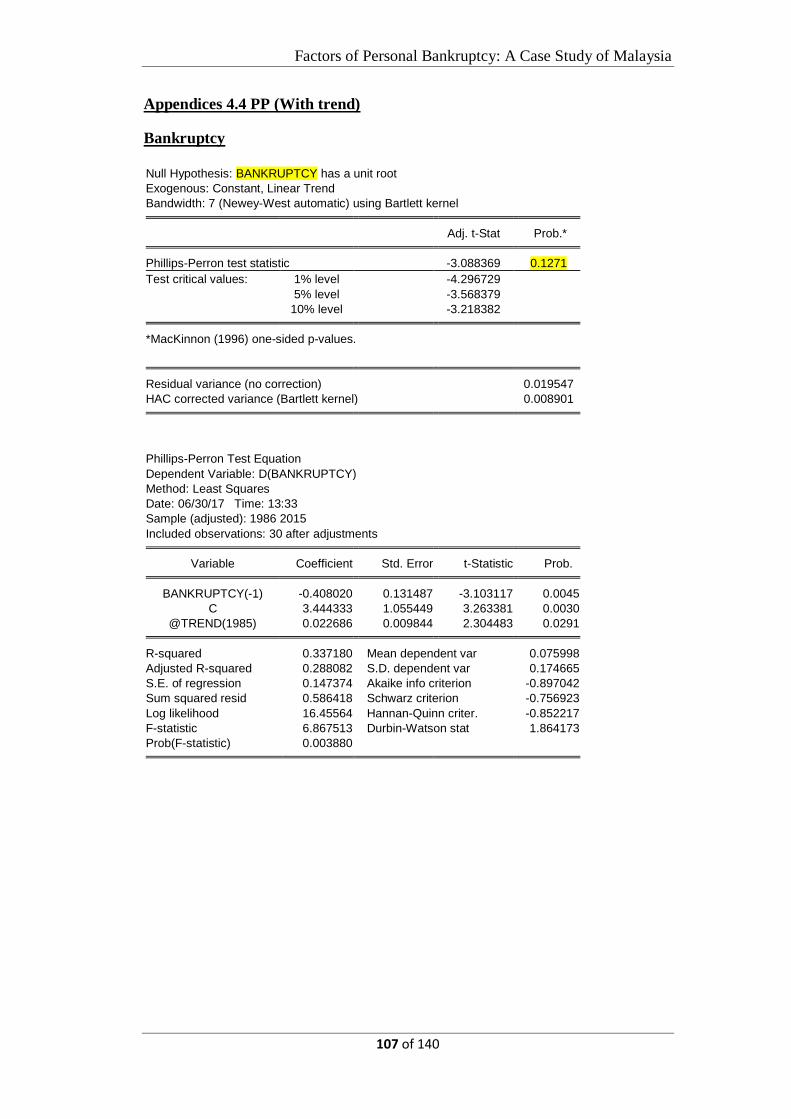
Factors of Personal Bankruptcy: A Case Study of Malaysia
107 of 140
Appendices 4.4 PP (With trend)
Bankruptcy
Null Hypothesis: BANKRUPTCY has a unit root
Exogenous: Constant, Linear Trend
Bandwidth: 7 (Newey-West automatic) using Bartlett kernel Adj. t-Stat Prob.* Phillips-Perron test statistic -3.088369 0.1271
Test critical values: 1% level -4.296729
5% level -3.568379
10% level -3.218382 *MacKinnon (1996) one-sided p-values.
Residual variance (no correction) 0.019547
HAC corrected variance (Bartlett kernel) 0.008901
Phillips-Perron Test Equation
Dependent Variable: D(BANKRUPTCY)
Method: Least Squares
Date: 06/30/17 Time: 13:33
Sample (adjusted): 1986 2015
Included observations: 30 after adjustments Variable Coefficient Std. Error t-Statistic Prob. BANKRUPTCY(-1) -0.408020 0.131487 -3.103117 0.0045
C 3.444333 1.055449 3.263381 0.0030
@TREND(1985) 0.022686 0.009844 2.304483 0.0291 R-squared 0.337180 Mean dependent var 0.075998
Adjusted R-squared 0.288082 S.D. dependent var 0.174665
S.E. of regression 0.147374 Akaike info criterion -0.897042
Sum squared resid 0.586418 Schwarz criterion -0.756923
Log likelihood 16.45564 Hannan-Quinn criter. -0.852217
F-statistic 6.867513 Durbin-Watson stat 1.864173
Prob(F-statistic) 0.003880

Factors of Personal Bankruptcy: A Case Study of Malaysia
108 of 140
Unemployment
Null Hypothesis: UNEMPLOYMENT has a unit root
Exogenous: Constant, Linear Trend
Bandwidth: 1 (Newey-West automatic) using Bartlett kernel Adj. t-Stat Prob.* Phillips-Perron test statistic -1.343889 0.8567
Test critical values: 1% level -4.296729
5% level -3.568379
10% level -3.218382 *MacKinnon (1996) one-sided p-values.
Residual variance (no correction) 0.289616
HAC corrected variance (Bartlett kernel) 0.375459
Phillips-Perron Test Equation
Dependent Variable: D(UNEMPLOYMENT)
Method: Least Squares
Date: 06/30/17 Time: 13:35
Sample (adjusted): 1986 2015
Included observations: 30 after adjustments Variable Coefficient Std. Error t-Statistic Prob. UNEMPLOYMENT(-1) -0.098476 0.083642 -1.177356 0.2493
C 0.267196 0.554228 0.482105 0.6336
@TREND(1985) 0.000534 0.016321 0.032726 0.9741 R-squared 0.090245 Mean dependent var -0.124667
Adjusted R-squared 0.022855 S.D. dependent var 0.573866
S.E. of regression 0.567270 Akaike info criterion 1.798677
Sum squared resid 8.688478 Schwarz criterion 1.938797
Log likelihood -23.98016 Hannan-Quinn criter. 1.843503
F-statistic 1.339156 Durbin-Watson stat 1.032030
Prob(F-statistic) 0.278921

Factors of Personal Bankruptcy: A Case Study of Malaysia
109 of 140
Lending
Null Hypothesis: LENDING has a unit root
Exogenous: Constant, Linear Trend
Bandwidth: 5 (Newey-West automatic) using Bartlett kernel Adj. t-Stat Prob.* Phillips-Perron test statistic -2.375723 0.3838
Test critical values: 1% level -4.296729
5% level -3.568379
10% level -3.218382 *MacKinnon (1996) one-sided p-values.
Residual variance (no correction) 0.620584
HAC corrected variance (Bartlett kernel) 0.569246
Phillips-Perron Test Equation
Dependent Variable: D(LENDING)
Method: Least Squares
Date: 06/30/17 Time: 13:40
Sample (adjusted): 1986 2015
Included observations: 30 after adjustments Variable Coefficient Std. Error t-Statistic Prob. LENDING(-1) -0.358715 0.146543 -2.447847 0.0212
C 1.517877 0.636024 2.386510 0.0243
@TREND(1985) 0.081604 0.036900 2.211469 0.0357 R-squared 0.181976 Mean dependent var 0.192333
Adjusted R-squared 0.121381 S.D. dependent var 0.885888
S.E. of regression 0.830384 Akaike info criterion 2.560783
Sum squared resid 18.61752 Schwarz criterion 2.700903
Log likelihood -35.41174 Hannan-Quinn criter. 2.605608
F-statistic 3.003180 Durbin-Watson stat 1.631513
Prob(F-statistic) 0.066427

Factors of Personal Bankruptcy: A Case Study of Malaysia
110 of 140
Divorce
Null Hypothesis: DIVORCE has a unit root
Exogenous: Constant, Linear Trend
Bandwidth: 4 (Newey-West automatic) using Bartlett kernel Adj. t-Stat Prob.* Phillips-Perron test statistic -2.204199 0.4703
Test critical values: 1% level -4.296729
5% level -3.568379
10% level -3.218382 *MacKinnon (1996) one-sided p-values.
Residual variance (no correction) 0.004909
HAC corrected variance (Bartlett kernel) 0.005931
Phillips-Perron Test Equation
Dependent Variable: D(DIVORCE)
Method: Least Squares
Date: 06/30/17 Time: 13:42
Sample (adjusted): 1986 2015
Included observations: 30 after adjustments Variable Coefficient Std. Error t-Statistic Prob. DIVORCE(-1) -0.190950 0.088361 -2.161038 0.0397
C 1.684592 0.761814 2.211291 0.0357
@TREND(1985) 0.016593 0.007038 2.357746 0.0259 R-squared 0.180549 Mean dependent var 0.066674
Adjusted R-squared 0.119849 S.D. dependent var 0.078720
S.E. of regression 0.073852 Akaike info criterion -2.278856
Sum squared resid 0.147263 Schwarz criterion -2.138736
Log likelihood 37.18283 Hannan-Quinn criter. -2.234030
F-statistic 2.974438 Durbin-Watson stat 2.122812
Prob(F-statistic) 0.068008

Factors of Personal Bankruptcy: A Case Study of Malaysia
111 of 140
Appendices 4.5 ADF (without trend) (First difference)
Bankruptcy
Null Hypothesis: D(BANKRUPTCY) has a unit root
Exogenous: Constant
Lag Length: 0 (Automatic - based on SIC, maxlag=7) t-Statistic Prob.* Augmented Dickey-Fuller test statistic -4.642881 0.0009
Test critical values: 1% level -3.679322
5% level -2.967767
10% level -2.622989 *MacKinnon (1996) one-sided p-values.
Augmented Dickey-Fuller Test Equation
Dependent Variable: D(BANKRUPTCY,2)
Method: Least Squares
Date: 06/30/17 Time: 13:23
Sample (adjusted): 1987 2015
Included observations: 29 after adjustments Variable Coefficient Std. Error t-Statistic Prob. D(BANKRUPTCY(-1)) -0.927237 0.199712 -4.642881 0.0001
C 0.067149 0.037494 1.790929 0.0845 R-squared 0.443945 Mean dependent var -0.011804
Adjusted R-squared 0.423350 S.D. dependent var 0.236971
S.E. of regression 0.179950 Akaike info criterion -0.525809
Sum squared resid 0.874309 Schwarz criterion -0.431513
Log likelihood 9.624229 Hannan-Quinn criter. -0.496276
F-statistic 21.55635 Durbin-Watson stat 1.773733
Prob(F-statistic) 0.000080

Factors of Personal Bankruptcy: A Case Study of Malaysia
112 of 140
Unemployment
Null Hypothesis: D(UNEMPLOYMENT) has a unit root
Exogenous: Constant
Lag Length: 0 (Automatic - based on SIC, maxlag=7) t-Statistic Prob.* Augmented Dickey-Fuller test statistic -4.175002 0.0030
Test critical values: 1% level -3.679322
5% level -2.967767
10% level -2.622989 *MacKinnon (1996) one-sided p-values.
Augmented Dickey-Fuller Test Equation
Dependent Variable: D(UNEMPLOYMENT,2)
Method: Least Squares
Date: 06/30/17 Time: 13:23
Sample (adjusted): 1987 2015
Included observations: 29 after adjustments Variable Coefficient Std. Error t-Statistic Prob. D(UNEMPLOYMENT(-1)) -0.647063 0.154985 -4.175002 0.0003
C -0.127039 0.090676 -1.401026 0.1726 R-squared 0.392311 Mean dependent var -0.036897
Adjusted R-squared 0.369804 S.D. dependent var 0.597418
S.E. of regression 0.474259 Akaike info criterion 1.412347
Sum squared resid 6.072889 Schwarz criterion 1.506643
Log likelihood -18.47903 Hannan-Quinn criter. 1.441879
F-statistic 17.43064 Durbin-Watson stat 1.727296
Prob(F-statistic) 0.000278

Factors of Personal Bankruptcy: A Case Study of Malaysia
113 of 140
Lending
Null Hypothesis: D(LENDING) has a unit root
Exogenous: Constant
Lag Length: 0 (Automatic - based on SIC, maxlag=7) t-Statistic Prob.* Augmented Dickey-Fuller test statistic -4.864413 0.0005
Test critical values: 1% level -3.679322
5% level -2.967767
10% level -2.622989 *MacKinnon (1996) one-sided p-values.
Augmented Dickey-Fuller Test Equation
Dependent Variable: D(LENDING,2)
Method: Least Squares
Date: 06/30/17 Time: 13:24
Sample (adjusted): 1987 2015
Included observations: 29 after adjustments Variable Coefficient Std. Error t-Statistic Prob. D(LENDING(-1)) -0.950675 0.195435 -4.864413 0.0000
C 0.190955 0.173081 1.103269 0.2796 R-squared 0.467062 Mean dependent var 0.036552
Adjusted R-squared 0.447323 S.D. dependent var 1.232490
S.E. of regression 0.916260 Akaike info criterion 2.729440
Sum squared resid 22.66739 Schwarz criterion 2.823736
Log likelihood -37.57688 Hannan-Quinn criter. 2.758972
F-statistic 23.66251 Durbin-Watson stat 1.956477
Prob(F-statistic) 0.000044

Factors of Personal Bankruptcy: A Case Study of Malaysia
114 of 140
Divorce
Null Hypothesis: D(DIVORCE) has a unit root
Exogenous: Constant
Lag Length: 0 (Automatic - based on SIC, maxlag=7) t-Statistic Prob.* Augmented Dickey-Fuller test statistic -5.610312 0.0001
Test critical values: 1% level -3.679322
5% level -2.967767
10% level -2.622989 *MacKinnon (1996) one-sided p-values.
Augmented Dickey-Fuller Test Equation
Dependent Variable: D(DIVORCE,2)
Method: Least Squares
Date: 06/30/17 Time: 13:25
Sample (adjusted): 1987 2015
Included observations: 29 after adjustments Variable Coefficient Std. Error t-Statistic Prob. D(DIVORCE(-1)) -1.074843 0.191584 -5.610312 0.0000
C 0.073984 0.019904 3.717124 0.0009 R-squared 0.538269 Mean dependent var 0.000164
Adjusted R-squared 0.521168 S.D. dependent var 0.116220
S.E. of regression 0.080422 Akaike info criterion -2.136594
Sum squared resid 0.174626 Schwarz criterion -2.042298
Log likelihood 32.98062 Hannan-Quinn criter. -2.107062
F-statistic 31.47560 Durbin-Watson stat 1.991547
Prob(F-statistic) 0.000006
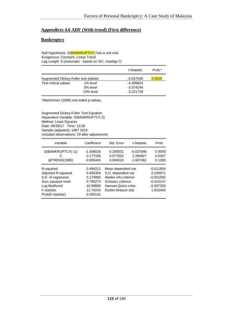
Factors of Personal Bankruptcy: A Case Study of Malaysia
115 of 140
Appendices 4.6 ADF (With trend) (First difference)
Bankruptcy
Null Hypothesis: D(BANKRUPTCY) has a unit root
Exogenous: Constant, Linear Trend
Lag Length: 0 (Automatic - based on SIC, maxlag=7) t-Statistic Prob.* Augmented Dickey-Fuller test statistic -5.027546 0.0018
Test critical values: 1% level -4.309824
5% level -3.574244
10% level -3.221728 *MacKinnon (1996) one-sided p-values.
Augmented Dickey-Fuller Test Equation
Dependent Variable: D(BANKRUPTCY,2)
Method: Least Squares
Date: 06/30/17 Time: 13:28
Sample (adjusted): 1987 2015
Included observations: 29 after adjustments Variable Coefficient Std. Error t-Statistic Prob. D(BANKRUPTCY(-1)) -1.008026 0.200501 -5.027546 0.0000
C 0.177156 0.077532 2.284927 0.0307
@TREND(1985) -0.006445 0.004010 -1.607462 0.1200 R-squared 0.494211 Mean dependent var -0.011804
Adjusted R-squared 0.455304 S.D. dependent var 0.236971
S.E. of regression 0.174893 Akaike info criterion -0.551592
Sum squared resid 0.795273 Schwarz criterion -0.410147
Log likelihood 10.99808 Hannan-Quinn criter. -0.507293
F-statistic 12.70243 Durbin-Watson stat 1.816430
Prob(F-statistic) 0.000142

Factors of Personal Bankruptcy: A Case Study of Malaysia
116 of 140
Unemployment
Null Hypothesis: D(UNEMPLOYMENT) has a unit root
Exogenous: Constant, Linear Trend
Lag Length: 0 (Automatic - based on SIC, maxlag=7) t-Statistic Prob.* Augmented Dickey-Fuller test statistic -4.813219 0.0031
Test critical values: 1% level -4.309824
5% level -3.574244
10% level -3.221728 *MacKinnon (1996) one-sided p-values.
Augmented Dickey-Fuller Test Equation
Dependent Variable: D(UNEMPLOYMENT,2)
Method: Least Squares
Date: 06/30/17 Time: 13:28
Sample (adjusted): 1987 2015
Included observations: 29 after adjustments Variable Coefficient Std. Error t-Statistic Prob. D(UNEMPLOYMENT(-1)) -0.705451 0.146565 -4.813219 0.0001
C -0.496646 0.183432 -2.707525 0.0118
@TREND(1985) 0.022592 0.009954 2.269589 0.0318 R-squared 0.492797 Mean dependent var -0.036897
Adjusted R-squared 0.453781 S.D. dependent var 0.597418
S.E. of regression 0.441531 Akaike info criterion 1.300561
Sum squared resid 5.068695 Schwarz criterion 1.442006
Log likelihood -15.85814 Hannan-Quinn criter. 1.344860
F-statistic 12.63075 Durbin-Watson stat 1.951212
Prob(F-statistic) 0.000147

Factors of Personal Bankruptcy: A Case Study of Malaysia
117 of 140
Lending
Null Hypothesis: D(LENDING) has a unit root
Exogenous: Constant, Linear Trend
Lag Length: 0 (Automatic - based on SIC, maxlag=7) t-Statistic Prob.* Augmented Dickey-Fuller test statistic -4.767967 0.0034
Test critical values: 1% level -4.309824
5% level -3.574244
10% level -3.221728 *MacKinnon (1996) one-sided p-values.
Augmented Dickey-Fuller Test Equation
Dependent Variable: D(LENDING,2)
Method: Least Squares
Date: 06/30/17 Time: 13:29
Sample (adjusted): 1987 2015
Included observations: 29 after adjustments Variable Coefficient Std. Error t-Statistic Prob. D(LENDING(-1)) -0.950257 0.199300 -4.767967 0.0001
C 0.173134 0.376898 0.459366 0.6498
@TREND(1985) 0.001110 0.020738 0.053502 0.9577 R-squared 0.467120 Mean dependent var 0.036552
Adjusted R-squared 0.426129 S.D. dependent var 1.232490
S.E. of regression 0.933663 Akaike info criterion 2.798295
Sum squared resid 22.66490 Schwarz criterion 2.939740
Log likelihood -37.57528 Hannan-Quinn criter. 2.842594
F-statistic 11.39575 Durbin-Watson stat 1.957295
Prob(F-statistic) 0.000279

Factors of Personal Bankruptcy: A Case Study of Malaysia
118 of 140
Divorce
Null Hypothesis: D(DIVORCE) has a unit root
Exogenous: Constant, Linear Trend
Lag Length: 0 (Automatic - based on SIC, maxlag=7) t-Statistic Prob.* Augmented Dickey-Fuller test statistic -5.662717 0.0004
Test critical values: 1% level -4.309824
5% level -3.574244
10% level -3.221728 *MacKinnon (1996) one-sided p-values.
Augmented Dickey-Fuller Test Equation
Dependent Variable: D(DIVORCE,2)
Method: Least Squares
Date: 06/30/17 Time: 13:30
Sample (adjusted): 1987 2015
Included observations: 29 after adjustments Variable Coefficient Std. Error t-Statistic Prob. D(DIVORCE(-1)) -1.123644 0.198428 -5.662717 0.0000
C 0.048860 0.032838 1.487917 0.1488
@TREND(1985) 0.001780 0.001849 0.962678 0.3446 R-squared 0.554161 Mean dependent var 0.000164
Adjusted R-squared 0.519865 S.D. dependent var 0.116220
S.E. of regression 0.080531 Akaike info criterion -2.102652
Sum squared resid 0.168616 Schwarz criterion -1.961208
Log likelihood 33.48846 Hannan-Quinn criter. -2.058354
F-statistic 16.15848 Durbin-Watson stat 1.959598
Prob(F-statistic) 0.000027

Factors of Personal Bankruptcy: A Case Study of Malaysia
119 of 140
Appendices 4.7 PP (Without trend) (First difference)
Bankruptcy
Null Hypothesis: D(BANKRUPTCY) has a unit root
Exogenous: Constant
Bandwidth: 7 (Newey-West automatic) using Bartlett kernel Adj. t-Stat Prob.* Phillips-Perron test statistic -4.549401 0.0011
Test critical values: 1% level -3.679322
5% level -2.967767
10% level -2.622989 *MacKinnon (1996) one-sided p-values.
Residual variance (no correction) 0.030149
HAC corrected variance (Bartlett kernel) 0.018379
Phillips-Perron Test Equation
Dependent Variable: D(BANKRUPTCY,2)
Method: Least Squares
Date: 06/30/17 Time: 13:32
Sample (adjusted): 1987 2015
Included observations: 29 after adjustments Variable Coefficient Std. Error t-Statistic Prob. D(BANKRUPTCY(-1)) -0.927237 0.199712 -4.642881 0.0001
C 0.067149 0.037494 1.790929 0.0845 R-squared 0.443945 Mean dependent var -0.011804
Adjusted R-squared 0.423350 S.D. dependent var 0.236971
S.E. of regression 0.179950 Akaike info criterion -0.525809
Sum squared resid 0.874309 Schwarz criterion -0.431513
Log likelihood 9.624229 Hannan-Quinn criter. -0.496276
F-statistic 21.55635 Durbin-Watson stat 1.773733
Prob(F-statistic) 0.000080

Factors of Personal Bankruptcy: A Case Study of Malaysia
120 of 140
Unemployment
Null Hypothesis: D(UNEMPLOYMENT) has a unit root
Exogenous: Constant
Bandwidth: 4 (Newey-West automatic) using Bartlett kernel Adj. t-Stat Prob.* Phillips-Perron test statistic -4.305127 0.0021
Test critical values: 1% level -3.679322
5% level -2.967767
10% level -2.622989 *MacKinnon (1996) one-sided p-values.
Residual variance (no correction) 0.209410
HAC corrected variance (Bartlett kernel) 0.320832
Phillips-Perron Test Equation
Dependent Variable: D(UNEMPLOYMENT,2)
Method: Least Squares
Date: 06/30/17 Time: 13:34
Sample (adjusted): 1987 2015
Included observations: 29 after adjustments Variable Coefficient Std. Error t-Statistic Prob. D(UNEMPLOYMENT(-1)) -0.647063 0.154985 -4.175002 0.0003
C -0.127039 0.090676 -1.401026 0.1726 R-squared 0.392311 Mean dependent var -0.036897
Adjusted R-squared 0.369804 S.D. dependent var 0.597418
S.E. of regression 0.474259 Akaike info criterion 1.412347
Sum squared resid 6.072889 Schwarz criterion 1.506643
Log likelihood -18.47903 Hannan-Quinn criter. 1.441879
F-statistic 17.43064 Durbin-Watson stat 1.727296
Prob(F-statistic) 0.000278

Factors of Personal Bankruptcy: A Case Study of Malaysia
121 of 140
Lending Null Hypothesis: D(LENDING) has a unit root
Exogenous: Constant
Bandwidth: 22 (Newey-West automatic) using Bartlett kernel Adj. t-Stat Prob.* Phillips-Perron test statistic -7.257031 0.0000
Test critical values: 1% level -3.679322
5% level -2.967767
10% level -2.622989 *MacKinnon (1996) one-sided p-values.
Residual variance (no correction) 0.781634
HAC corrected variance (Bartlett kernel) 0.088283
Phillips-Perron Test Equation
Dependent Variable: D(LENDING,2)
Method: Least Squares
Date: 06/30/17 Time: 13:39
Sample (adjusted): 1987 2015
Included observations: 29 after adjustments Variable Coefficient Std. Error t-Statistic Prob. D(LENDING(-1)) -0.950675 0.195435 -4.864413 0.0000
C 0.190955 0.173081 1.103269 0.2796 R-squared 0.467062 Mean dependent var 0.036552
Adjusted R-squared 0.447323 S.D. dependent var 1.232490
S.E. of regression 0.916260 Akaike info criterion 2.729440
Sum squared resid 22.66739 Schwarz criterion 2.823736
Log likelihood -37.57688 Hannan-Quinn criter. 2.758972
F-statistic 23.66251 Durbin-Watson stat 1.956477
Prob(F-statistic) 0.000044

Factors of Personal Bankruptcy: A Case Study of Malaysia
122 of 140
Divorce
Null Hypothesis: D(DIVORCE) has a unit root
Exogenous: Constant
Bandwidth: 4 (Newey-West automatic) using Bartlett kernel Adj. t-Stat Prob.* Phillips-Perron test statistic -5.655741 0.0001
Test critical values: 1% level -3.679322
5% level -2.967767
10% level -2.622989 *MacKinnon (1996) one-sided p-values.
Residual variance (no correction) 0.006022
HAC corrected variance (Bartlett kernel) 0.008618
Phillips-Perron Test Equation
Dependent Variable: D(DIVORCE,2)
Method: Least Squares
Date: 06/30/17 Time: 13:42
Sample (adjusted): 1987 2015
Included observations: 29 after adjustments Variable Coefficient Std. Error t-Statistic Prob. D(DIVORCE(-1)) -1.074843 0.191584 -5.610312 0.0000
C 0.073984 0.019904 3.717124 0.0009 R-squared 0.538269 Mean dependent var 0.000164
Adjusted R-squared 0.521168 S.D. dependent var 0.116220
S.E. of regression 0.080422 Akaike info criterion -2.136594
Sum squared resid 0.174626 Schwarz criterion -2.042298
Log likelihood 32.98062 Hannan-Quinn criter. -2.107062
F-statistic 31.47560 Durbin-Watson stat 1.991547
Prob(F-statistic) 0.000006

Factors of Personal Bankruptcy: A Case Study of Malaysia
123 of 140
Appendices 4.8 PP (With trend)
Bankruptcy
Null Hypothesis: D(BANKRUPTCY) has a unit root
Exogenous: Constant, Linear Trend
Bandwidth: 9 (Newey-West automatic) using Bartlett kernel Adj. t-Stat Prob.* Phillips-Perron test statistic -5.413289 0.0007
Test critical values: 1% level -4.309824
5% level -3.574244
10% level -3.221728 *MacKinnon (1996) one-sided p-values.
Residual variance (no correction) 0.027423
HAC corrected variance (Bartlett kernel) 0.010155
Phillips-Perron Test Equation
Dependent Variable: D(BANKRUPTCY,2)
Method: Least Squares
Date: 06/30/17 Time: 13:33
Sample (adjusted): 1987 2015
Included observations: 29 after adjustments Variable Coefficient Std. Error t-Statistic Prob. D(BANKRUPTCY(-1)) -1.008026 0.200501 -5.027546 0.0000
C 0.177156 0.077532 2.284927 0.0307
@TREND(1985) -0.006445 0.004010 -1.607462 0.1200 R-squared 0.494211 Mean dependent var -0.011804
Adjusted R-squared 0.455304 S.D. dependent var 0.236971
S.E. of regression 0.174893 Akaike info criterion -0.551592
Sum squared resid 0.795273 Schwarz criterion -0.410147
Log likelihood 10.99808 Hannan-Quinn criter. -0.507293
F-statistic 12.70243 Durbin-Watson stat 1.816430
Prob(F-statistic) 0.000142

Factors of Personal Bankruptcy: A Case Study of Malaysia
124 of 140
Unemployment
Null Hypothesis: D(UNEMPLOYMENT) has a unit root
Exogenous: Constant, Linear Trend
Bandwidth: 3 (Newey-West automatic) using Bartlett kernel Adj. t-Stat Prob.* Phillips-Perron test statistic -4.801628 0.0031
Test critical values: 1% level -4.309824
5% level -3.574244
10% level -3.221728 *MacKinnon (1996) one-sided p-values.
Residual variance (no correction) 0.174783
HAC corrected variance (Bartlett kernel) 0.180258
Phillips-Perron Test Equation
Dependent Variable: D(UNEMPLOYMENT,2)
Method: Least Squares
Date: 06/30/17 Time: 13:35
Sample (adjusted): 1987 2015
Included observations: 29 after adjustments Variable Coefficient Std. Error t-Statistic Prob. D(UNEMPLOYMENT(-1)) -0.705451 0.146565 -4.813219 0.0001
C -0.496646 0.183432 -2.707525 0.0118
@TREND(1985) 0.022592 0.009954 2.269589 0.0318 R-squared 0.492797 Mean dependent var -0.036897
Adjusted R-squared 0.453781 S.D. dependent var 0.597418
S.E. of regression 0.441531 Akaike info criterion 1.300561
Sum squared resid 5.068695 Schwarz criterion 1.442006
Log likelihood -15.85814 Hannan-Quinn criter. 1.344860
F-statistic 12.63075 Durbin-Watson stat 1.951212
Prob(F-statistic) 0.000147

Factors of Personal Bankruptcy: A Case Study of Malaysia
125 of 140
Lending
Null Hypothesis: D(LENDING) has a unit root
Exogenous: Constant, Linear Trend
Bandwidth: 21 (Newey-West automatic) using Bartlett kernel Adj. t-Stat Prob.* Phillips-Perron test statistic -6.790847 0.0000
Test critical values: 1% level -4.309824
5% level -3.574244
10% level -3.221728 *MacKinnon (1996) one-sided p-values.
Residual variance (no correction) 0.781548
HAC corrected variance (Bartlett kernel) 0.094630
Phillips-Perron Test Equation
Dependent Variable: D(LENDING,2)
Method: Least Squares
Date: 06/30/17 Time: 13:40
Sample (adjusted): 1987 2015
Included observations: 29 after adjustments Variable Coefficient Std. Error t-Statistic Prob. D(LENDING(-1)) -0.950257 0.199300 -4.767967 0.0001
C 0.173134 0.376898 0.459366 0.6498
@TREND(1985) 0.001110 0.020738 0.053502 0.9577 R-squared 0.467120 Mean dependent var 0.036552
Adjusted R-squared 0.426129 S.D. dependent var 1.232490
S.E. of regression 0.933663 Akaike info criterion 2.798295
Sum squared resid 22.66490 Schwarz criterion 2.939740
Log likelihood -37.57528 Hannan-Quinn criter. 2.842594
F-statistic 11.39575 Durbin-Watson stat 1.957295
Prob(F-statistic) 0.000279

Factors of Personal Bankruptcy: A Case Study of Malaysia
126 of 140
Divorce
Null Hypothesis: D(DIVORCE) has a unit root
Exogenous: Constant, Linear Trend
Bandwidth: 4 (Newey-West automatic) using Bartlett kernel Adj. t-Stat Prob.* Phillips-Perron test statistic -5.699697 0.0004
Test critical values: 1% level -4.309824
5% level -3.574244
10% level -3.221728 *MacKinnon (1996) one-sided p-values.
Residual variance (no correction) 0.005814
HAC corrected variance (Bartlett kernel) 0.007978
Phillips-Perron Test Equation
Dependent Variable: D(DIVORCE,2)
Method: Least Squares
Date: 06/30/17 Time: 13:43
Sample (adjusted): 1987 2015
Included observations: 29 after adjustments Variable Coefficient Std. Error t-Statistic Prob. D(DIVORCE(-1)) -1.123644 0.198428 -5.662717 0.0000
C 0.048860 0.032838 1.487917 0.1488
@TREND(1985) 0.001780 0.001849 0.962678 0.3446 R-squared 0.554161 Mean dependent var 0.000164
Adjusted R-squared 0.519865 S.D. dependent var 0.116220
S.E. of regression 0.080531 Akaike info criterion -2.102652
Sum squared resid 0.168616 Schwarz criterion -1.961208
Log likelihood 33.48846 Hannan-Quinn criter. -2.058354
F-statistic 16.15848 Durbin-Watson stat 1.959598
Prob(F-statistic) 0.000027

Factors of Personal Bankruptcy: A Case Study of Malaysia
127 of 140
Appendices 4.9 Multicollinearity
Divorce Lending Unemployment
Divorce 1.000000 0.875662 -0.557647
Lending 0.875662 1.000000 -0.550533
Unemployment -0.557647 -0.557647 1.000000
Correlation analysis
Dependent
variable
Independent
variable
R-Squared VIF=
Lending Divorce 0.766785 1.000000
Dependent
variable
Independent
variable
R-squared VIF
Divorce Lending 0.766785 1.000000
Dependent Variable: LENDING
Method: Least Squares
Date: 05/06/17 Time: 22:03
Sample: 1985 2015
Included observations: 31 Variable Coefficient Std. Error t-Statistic Prob. DIVORCE 2.736190 0.280214 9.764657 0.0000
C -19.64931 2.769326 -7.095341 0.0000 R-squared 0.766785 Mean dependent var 7.322581
Adjusted R-squared 0.758743 S.D. dependent var 2.251206
S.E. of regression 1.105746 Akaike info criterion 3.101259
Sum squared resid 35.45757 Schwarz criterion 3.193774
Log likelihood -46.06951 Hannan-Quinn criter. 3.131416
F-statistic 95.34852 Durbin-Watson stat 0.612587
Prob(F-statistic) 0.000000

Factors of Personal Bankruptcy: A Case Study of Malaysia
128 of 140
Variance Inflation Factors
Date: 05/06/17 Time: 21:42
Sample: 1985 2015
Included observations: 31 Coefficient Uncentered Centered
Variable Variance VIF VIF DIVORCE 0.078520 194.4459 1.000000
C 7.669164 194.4459 NA
Conclusion: Multi happen but not a serious multi problem
Appendices 4.10 Heteroscedasticity
Heteroskedasticity Test: ARCH F-statistic 3.032021 Prob. F(1,28) 0.0926
Obs*R-squared 2.931187 Prob. Chi-Square(1) 0.0869
Test Equation:
Dependent Variable: RESID^2
Method: Least Squares
Date: 05/06/17 Time: 21:44
Sample (adjusted): 1986 2015
Included observations: 30 after adjustments Variable Coefficient Std. Error t-Statistic Prob. C 0.031314 0.009316 3.361440 0.0023
RESID^2(-1) 0.165420 0.095000 1.741270 0.0926 R-squared 0.097706 Mean dependent var 0.040198
Adjusted R-squared 0.065481 S.D. dependent var 0.044162
S.E. of regression 0.042692 Akaike info criterion -3.405290
Sum squared resid 0.051032 Schwarz criterion -3.311877
Log likelihood 53.07935 Hannan-Quinn criter. -3.375406
F-statistic 3.032021 Durbin-Watson stat 2.120376
Prob(F-statistic) 0.092615

Factors of Personal Bankruptcy: A Case Study of Malaysia
129 of 140
Appendices 4.11 Specification bias
Ramsey RESET Test
Equation: UNTITLED
Specification: BANKRUPTCY DIVORCE LENDING UNEMPLOYMENT C
Omitted Variables: Squares of fitted values Value df Probability
t-statistic 1.856965 26 0.0747
F-statistic 3.448318 (1, 26) 0.0747
Likelihood ratio 3.860748 1 0.0494 F-test summary:
Sum of Sq. df Mean
Squares
Test SSR 0.191444 1 0.191444
Restricted SSR 1.634911 27 0.060552
Unrestricted SSR 1.443468 26 0.055518
Unrestricted SSR 1.443468 26 0.055518 LR test summary:
Value df
Restricted LogL 1.620086 27
Unrestricted LogL 3.550459 26
Unrestricted Test Equation:
Dependent Variable: BANKRUPTCY
Method: Least Squares
Date: 05/06/17 Time: 21:44
Sample: 1985 2015
Included observations: 31 Variable Coefficient Std. Error t-Statistic Prob. DIVORCE 6.227524 3.117993 1.997286 0.0564
LENDING 0.993736 0.495841 2.004143 0.0556
UNEMPLOYMENT -1.476638 0.730185 -2.022279 0.0535
C 3.640609 1.204311 3.022980 0.0056
FITTED^2 -0.681807 0.367162 -1.856965 0.0747 R-squared 0.889647 Mean dependent var 9.139907
Adjusted R-squared 0.872670 S.D. dependent var 0.660315
S.E. of regression 0.235623 Akaike info criterion 0.093519
Sum squared resid 1.443468 Schwarz criterion 0.324807
Log likelihood 3.550459 Hannan-Quinn criter. 0.168913
F-statistic 52.40202 Durbin-Watson stat 0.858828
Prob(F-statistic) 0.000000
Conclusion: No specification bias

Factors of Personal Bankruptcy: A Case Study of Malaysia
130 of 140
Appendices 4.12 Normality test
Conclusion: Error term is normally distribute
Appendices 4.13Autocorrelation
Breusch-Godfrey Serial Correlation LM Test: F-statistic 5.815723 Prob. F(2,25) 0.0084
Obs*R-squared 9.843314 Prob. Chi-Square(2) 0.0073
Test Equation:
Dependent Variable: RESID
Method: Least Squares
Date: 05/06/17 Time: 21:52
Sample: 1985 2015
Included observations: 31
Presample missing value lagged residuals set to zero. Variable Coefficient Std. Error t-Statistic Prob. DIVORCE 0.006409 0.120315 0.053267 0.9579
LENDING -0.001684 0.038288 -0.043980 0.9653
UNEMPLOYMENT 0.005010 0.028510 0.175737 0.8619
C -0.073578 1.006231 -0.073123 0.9423
RESID(-1) 0.655753 0.192288 3.410271 0.0022
RESID(-2) -0.320812 0.206370 -1.554550 0.1326 R-squared 0.317526 Mean dependent var -3.94E-15
Adjusted R-squared 0.181032 S.D. dependent var 0.233446
S.E. of regression 0.211261 Akaike info criterion -0.099456
Sum squared resid 1.115784 Schwarz criterion 0.178090
Log likelihood 7.541570 Hannan-Quinn criter. -0.008983
F-statistic 2.326289 Durbin-Watson stat 1.597173
Prob(F-statistic) 0.072642
Conclusion: Autocorrelation problem, proceed to apply Newey west
0
1
2
3
4
5
6
7
-0.6 -0.4 -0.2 0.0 0.2 0.4
Series: ResidualsSample 1985 2015Observations 31
Mean -3.94e-15Median 0.026544Maximum 0.422477Minimum -0.654949Std. Dev. 0.233446Skewness -0.496802Kurtosis 3.352222
Jarque-Bera 1.435440Probability 0.487863

Factors of Personal Bankruptcy: A Case Study of Malaysia
131 of 140
Newey west
Dependent Variable: BANKRUPTCY
Method: Least Squares
Date: 05/07/17 Time: 20:59
Sample: 1985 2015
Included observations: 31
HAC standard errors & covariance (Bartlett kernel, Newey-West fixed
bandwidth = 4.0000) Variable Coefficient Std. Error t-Statistic Prob. DIVORCE 0.442241 0.098053 4.510228 0.0001
LENDING 0.075986 0.022879 3.321195 0.0026
UNEMPLOYMENT -0.121926 0.044590 -2.734383 0.0109
C 4.715952 0.994437 4.742331 0.0001 R-squared 0.875011 Mean dependent var 9.139907
Adjusted R-squared 0.861124 S.D. dependent var 0.660315
S.E. of regression 0.246074 Akaike info criterion 0.153543
Sum squared resid 1.634911 Schwarz criterion 0.338573
Log likelihood 1.620086 Hannan-Quinn criter. 0.213858
F-statistic 63.00659 Durbin-Watson stat 0.760269
Prob(F-statistic) 0.000000
Appendices 4.14VAR Lag Order Selection Criteria
VAR Lag Order Selection Criteria Endogenous variables: BANKRUPTCY UNEMPLOYMENT LENDING DIVORCE
Exogenous variables: C
Date: 07/06/17 Time: 15:29
Sample: 1985 2015
Included observations: 29 Lag LogL LR FPE AIC SC HQ 0 -111.5861 NA 0.034049 7.971452 8.160045 8.030517
1 8.770430 199.2107* 2.59e-05* 0.774453 1.717416* 1.069777*
2 25.61924 23.23974 2.62e-05 0.715914* 2.413247 1.247498 * indicates lag order selected by the criterion
LR: sequential modified LR test statistic (each test at 5% level)
FPE: Final prediction error
AIC: Akaike information criterion
SC: Schwarz information criterion
HQ: Hannan-Quinn information criterion

Factors of Personal Bankruptcy: A Case Study of Malaysia
132 of 140
Appendices 4.15 Johansen Cointegration Test
Date: 07/03/17 Time: 20:30
Sample (adjusted): 1988 2015
Included observations: 28 after adjustments
Trend assumption: Linear deterministic trend
Series: BANKRUPTCY UNEMPLOYMENT LENDING DIVORCE
Lags interval (in first differences): 1 to 2
Unrestricted Cointegration Rank Test (Trace) Hypothesized Trace 0.05
No. of CE(s) Eigenvalue Statistic Critical Value Prob.** None * 0.751560 79.68842 47.85613 0.0000
At most 1 * 0.663688 40.69688 29.79707 0.0019
At most 2 0.302494 10.18481 15.49471 0.2668
At most 3 0.003492 0.097959 3.841466 0.7543 Trace test indicates 2 cointegrating eqn(s) at the 0.05 level
* denotes rejection of the hypothesis at the 0.05 level
**MacKinnon-Haug-Michelis (1999) p-values
Unrestricted Cointegration Rank Test (Maximum Eigenvalue) Hypothesized Max-Eigen 0.05
No. of CE(s) Eigenvalue Statistic Critical Value Prob.** None * 0.751560 38.99154 27.58434 0.0011
At most 1 * 0.663688 30.51207 21.13162 0.0018
At most 2 0.302494 10.08685 14.26460 0.2063
At most 3 0.003492 0.097959 3.841466 0.7543 Max-eigenvalue test indicates 2 cointegrating eqn(s) at the 0.05 level
* denotes rejection of the hypothesis at the 0.05 level
**MacKinnon-Haug-Michelis (1999) p-values
Unrestricted Cointegrating Coefficients (normalized by b'*S11*b=I):
BANKRUPTCY UNEMPLOYMEN
T LENDING DIVORCE
1.962585 0.143401 -1.847505 2.974486
-0.113787 1.015276 0.413888 -0.908062
-7.598632 -0.843871 0.449641 3.589783
-1.422300 0.394179 0.035537 2.830094
Unrestricted Adjustment Coefficients (alpha): D(BANKRUPTC
Y) 0.015853 0.045362 0.047878 -0.006226 D(UNEMPLOYM
ENT) -0.146783 -0.215778 0.003071 -0.008690
D(LENDING) 0.233562 0.051024 -0.308662 -0.028835
D(DIVORCE) -0.054406 0.009239 -0.017005 -0.001326
1 Cointegrating Equation(s): Log likelihood 26.41475 Normalized cointegrating coefficients (standard error in parentheses)

Factors of Personal Bankruptcy: A Case Study of Malaysia
133 of 140
BANKRUPTCY UNEMPLOYMEN
T LENDING DIVORCE
1.000000 0.073067 -0.941363 1.515596
(0.08022) (0.11933) (0.31232)
Adjustment coefficients (standard error in parentheses) D(BANKRUPTC
Y) 0.031113
(0.06840) D(UNEMPLOYM
ENT) -0.288075
(0.14550)
D(LENDING) 0.458386
(0.35077)
D(DIVORCE) -0.106776
(0.02344)
2 Cointegrating Equation(s): Log likelihood 41.67079 Normalized cointegrating coefficients (standard error in parentheses)
BANKRUPTCY UNEMPLOYMEN
T LENDING DIVORCE
1.000000 0.000000 -0.963261 1.568106
(0.11689) (0.31449)
0.000000 1.000000 0.299703 -0.718653
(0.27588) (0.74224)
Adjustment coefficients (standard error in parentheses) D(BANKRUPTC
Y) 0.025952 0.048328
(0.06521) (0.03401) D(UNEMPLOYM
ENT) -0.263522 -0.240123
(0.10604) (0.05531)
D(LENDING) 0.452580 0.085296
(0.35056) (0.18284)
D(DIVORCE) -0.107827 0.001578
(0.02308) (0.01204)
3 Cointegrating Equation(s): Log likelihood 46.71421 Normalized cointegrating coefficients (standard error in parentheses)
BANKRUPTCY UNEMPLOYMEN
T LENDING DIVORCE
1.000000 0.000000 0.000000 -0.600794
(0.09907)
0.000000 1.000000 0.000000 -0.043836
(0.30031)
0.000000 0.000000 1.000000 -2.251621
(0.17072)
Adjustment coefficients (standard error in parentheses) D(BANKRUPTC
Y) -0.337854 0.007926 0.011014
(0.24481) (0.04142) (0.06069) D(UNEMPLOYM
ENT) -0.286860 -0.242715 0.183256
(0.42332) (0.07162) (0.10495)
D(LENDING) 2.797990 0.345767 -0.549176
(1.27784) (0.21620) (0.31681)
D(DIVORCE) 0.021386 0.015928 0.096693

Factors of Personal Bankruptcy: A Case Study of Malaysia
134 of 140
(0.08662) (0.01466) (0.02148)
Appendices 4.16 VECM
Vector Error Correction Estimates
Date: 07/03/17 Time: 20:32
Sample (adjusted): 1988 2015
Included observations: 28 after adjustments
Standard errors in ( ) & t-statistics in [ ] Cointegrating Eq: CointEq1 BANKRUPTCY(-1) 1.000000
UNEMPLOYMENT(-1) 0.073067
(0.08022)
[ 0.91082]
LENDING(-1) -0.941363
(0.11933)
[-7.88849]
DIVORCE(-1) 1.515596
(0.31232)
[ 4.85264]
C -17.50095
Error Correction: D(BANKRUPTC
Y) D(UNEMPLOY
MENT) D(LENDING) D(DIVORCE) CointEq1 0.031113 -0.288075 0.458386 -0.106776
(0.06840) (0.14550) (0.35077) (0.02344)
[ 0.45490] [-1.97994] [ 1.30681] [-4.55610]
D(BANKRUPTCY(-1)) 0.007503 -0.473538 -1.426839 -0.026323
(0.23328) (0.49625) (1.19637) (0.07993)
[ 0.03216] [-0.95423] [-1.19264] [-0.32931]
D(BANKRUPTCY(-2)) -0.232918 -1.194955 -0.285089 0.006103
(0.22856) (0.48620) (1.17216) (0.07832)
[-1.01908] [-2.45772] [-0.24322] [ 0.07793]
D(UNEMPLOYMENT(-1)) -0.023675 0.687456 0.639131 0.048487
(0.09433) (0.20067) (0.48379) (0.03232)
[-0.25098] [ 3.42577] [ 1.32110] [ 1.50007]
D(UNEMPLOYMENT(-2)) 0.016892 -0.023443 -0.131594 -0.054247
(0.07789) (0.16569) (0.39946) (0.02669)
[ 0.21687] [-0.14149] [-0.32943] [-2.03259]
D(LENDING(-1)) 0.029201 -0.197853 0.289493 -0.038014
(0.05051) (0.10746) (0.25906) (0.01731)
[ 0.57808] [-1.84125] [ 1.11748] [-2.19628]

Factors of Personal Bankruptcy: A Case Study of Malaysia
135 of 140
D(LENDING(-2)) -0.023671 -0.046404 0.169101 -0.024956
(0.05040) (0.10721) (0.25847) (0.01727)
[-0.46968] [-0.43283] [ 0.65424] [-1.44511]
D(DIVORCE(-1)) -0.013861 -2.134220 -2.016886 -0.885870
(0.69609) (1.48079) (3.56993) (0.23852)
[-0.01991] [-1.44127] [-0.56496] [-3.71406]
D(DIVORCE(-2)) 0.174089 -4.905097 -1.710504 -0.567346
(0.63047) (1.34120) (3.23341) (0.21603)
[ 0.27612] [-3.65724] [-0.52901] [-2.62619]
C 0.063382 0.629195 0.643337 0.187367
(0.10694) (0.22749) (0.54844) (0.03664)
[ 0.59269] [ 2.76580] [ 1.17303] [ 5.11329] R-squared 0.121371 0.616491 0.290139 0.583868
Adj. R-squared -0.317944 0.424737 -0.064791 0.375802
Sum sq. resids 0.612107 2.770003 16.09954 0.071868
S.E. equation 0.184407 0.392287 0.945737 0.063188
F-statistic 0.276273 3.215002 0.817455 2.806164
Log likelihood 13.79245 -7.343294 -31.98249 43.78154
Akaike AIC -0.270889 1.238807 2.998749 -2.412967
Schwarz SC 0.204898 1.714594 3.474537 -1.937180
Mean dependent 0.058375 -0.180714 0.206071 0.070737
S.D. dependent 0.160631 0.517214 0.916512 0.079978 Determinant resid covariance (dof adj.) 1.04E-05
Determinant resid covariance 1.78E-06
Log likelihood 26.41475
Akaike information criterion 1.256089
Schwarz criterion 3.349553
Diagnostic checking for VECM
Appendices 4.17 Autocorrelation
VEC Residual Portmanteau Tests for Autocorrelations
Null Hypothesis: no residual autocorrelations up to lag h
Date: 07/05/17 Time: 19:44
Sample: 1985 2015
Included observations: 28 Lags Q-Stat Prob. Adj Q-Stat Prob. df 1 6.470236 NA* 6.709875 NA* NA*
2 14.39627 NA* 15.24561 NA* NA*
3 24.50845 0.6544 26.57124 0.5417 28
4 32.89024 0.8905 36.35000 0.7870 44
5 50.38473 0.8073 57.64764 0.5622 60
6 69.20769 0.6963 81.60413 0.3094 76
7 79.08842 0.8291 94.77844 0.4006 92
8 97.65776 0.7523 120.7755 0.1889 108
9 107.4960 0.8544 135.2740 0.2305 124
10 117.2118 0.9197 150.3874 0.2593 140

Factors of Personal Bankruptcy: A Case Study of Malaysia
136 of 140
11 130.9038 0.9288 172.9390 0.1676 156
12 137.2091 0.9763 183.9733 0.2524 172 *The test is valid only for lags larger than the VAR lag order.
df is degrees of freedom for (approximate) chi-square distribution
Appendices 4.18 Normality test
VEC Residual Normality Tests
Orthogonalization: Cholesky (Lutkepohl)
Null Hypothesis: residuals are multivariate normal
Date: 07/05/17 Time: 19:50
Sample: 1985 2015
Included observations: 28
Component Skewness Chi-sq df Prob. 1 0.864046 3.484019 1 0.0620
2 -0.723035 2.439637 1 0.1183
3 2.650268 32.77830 1 0.0000
4 -0.749190 2.619333 1 0.1056 Joint 41.32129 4 0.0000
Component Kurtosis Chi-sq df Prob. 1 5.443109 6.963576 1 0.0083
2 3.612633 0.437872 1 0.5082
3 11.74260 89.17188 1 0.0000
4 3.279199 0.090944 1 0.7630 Joint 96.66428 4 0.0000
Component Jarque-Bera df Prob. 1 10.44760 2 0.0054
2 2.877509 2 0.2372
3 121.9502 2 0.0000
4 2.710277 2 0.2579 Joint 137.9856 8 0.0000
Factors of Personal Bankruptcy: A Case Study of Malaysia
137 of 140
Appendices 4.19 Heteroscedasticity
VEC Residual Heteroskedasticity Tests: No Cross Terms (only levels and squares)
Date: 07/05/17 Time: 19:59
Sample: 1985 2015
Included observations: 28
Joint test: Chi-sq df Prob. 180.5474 180 0.4745
Individual components: Dependent R-squared F(18,9) Prob. Chi-sq(18) Prob. res1*res1 0.892078 4.132974 0.0174 24.97818 0.1255
res2*res2 0.845717 2.740797 0.0626 23.68008 0.1658
res3*res3 0.400139 0.333526 0.9773 11.20388 0.8855
res4*res4 0.651893 0.936338 0.5702 18.25299 0.4391
res2*res1 0.623167 0.826847 0.6521 17.44867 0.4925
res3*res1 0.431557 0.379595 0.9617 12.08359 0.8429
res3*res2 0.637487 0.879262 0.6121 17.84964 0.4656
res4*res1 0.543640 0.595627 0.8330 15.22193 0.6467
res4*res2 0.625626 0.835564 0.6454 17.51754 0.4878
res4*res3 0.400863 0.334533 0.9770 11.22416 0.8846

Factors of Personal Bankruptcy: A Case Study of Malaysia
138 of 140
Appendices 4.20 Granger Causality Test
VEC Granger Causality/Block Exogeneity Wald Tests
Date: 07/06/17 Time: 11:36
Sample: 1985 2015
Included observations: 28
Dependent variable: D(BANKRUPTCY) Excluded Chi-sq df Prob. D(UNEMPLOY
MENT) 0.075043 2 0.9632
D(LENDING) 0.740733 2 0.6905
D(DIVORCE) 0.110360 2 0.9463 All 0.817751 6 0.9916
Dependent variable: D(UNEMPLOYMENT) Excluded Chi-sq df Prob. D(BANKRUPT
CY) 6.427948 2 0.0402
D(LENDING) 3.391535 2 0.1835
D(DIVORCE) 13.59701 2 0.0011 All 19.45593 6 0.0035
Dependent variable: D(LENDING) Excluded Chi-sq df Prob. D(BANKRUPT
CY) 1.428804 2 0.4895 D(UNEMPLOY
MENT) 1.866506 2 0.3933
D(DIVORCE) 0.398863 2 0.8192 All 2.900230 6 0.8213
Dependent variable: D(DIVORCE) Excluded Chi-sq df Prob. D(BANKRUPT
CY) 0.123906 2 0.9399 D(UNEMPLOY
MENT) 4.487689 2 0.1060
D(LENDING) 5.664226 2 0.0589 All 10.48103 6 0.1058

Factors of Personal Bankruptcy: A Case Study of Malaysia
139 of 140
Appendices 4.21 Impulse Response Function
-.1
.0
.1
.2
1 2 3 4 5 6 7 8 9 10
Response of BANKRUPTCY to BANKRUPTCY
-.1
.0
.1
.2
1 2 3 4 5 6 7 8 9 10
Response of BANKRUPTCY to UNEMPLOYMENT
-.1
.0
.1
.2
1 2 3 4 5 6 7 8 9 10
Response of BANKRUPTCY to LENDING
-.1
.0
.1
.2
1 2 3 4 5 6 7 8 9 10
Response of BANKRUPTCY to DIVORCE
-1.0
-0.5
0.0
0.5
1.0
1.5
1 2 3 4 5 6 7 8 9 10
Response of UNEMPLOYMENT to BANKRUPTCY
-1.0
-0.5
0.0
0.5
1.0
1.5
1 2 3 4 5 6 7 8 9 10
Response of UNEMPLOYMENT to UNEMPLOYMENT
-1.0
-0.5
0.0
0.5
1.0
1.5
1 2 3 4 5 6 7 8 9 10
Response of UNEMPLOYMENT to LENDING
-1.0
-0.5
0.0
0.5
1.0
1.5
1 2 3 4 5 6 7 8 9 10
Response of UNEMPLOYMENT to DIVORCE
-0.4
0.0
0.4
0.8
1.2
1 2 3 4 5 6 7 8 9 10
Response of LENDING to BANKRUPTCY
-0.4
0.0
0.4
0.8
1.2
1 2 3 4 5 6 7 8 9 10
Response of LENDING to UNEMPLOYMENT
-0.4
0.0
0.4
0.8
1.2
1 2 3 4 5 6 7 8 9 10
Response of LENDING to LENDING
-0.4
0.0
0.4
0.8
1.2
1 2 3 4 5 6 7 8 9 10
Response of LENDING to DIVORCE
-.08
-.04
.00
.04
.08
.12
1 2 3 4 5 6 7 8 9 10
Response of DIVORCE to BANKRUPTCY
-.08
-.04
.00
.04
.08
.12
1 2 3 4 5 6 7 8 9 10
Response of DIVORCE to UNEMPLOYMENT
-.08
-.04
.00
.04
.08
.12
1 2 3 4 5 6 7 8 9 10
Response of DIVORCE to LENDING
-.08
-.04
.00
.04
.08
.12
1 2 3 4 5 6 7 8 9 10
Response of DIVORCE to DIVORCE
Response to Cholesky One S.D. Innov ations

Factors of Personal Bankruptcy: A Case Study of Malaysia
140 of 140
Appendices 5.1
Source: Bank Negara Malaysia (BNM)

Factors of Personal Bankruptcy: A Case Study of Malaysia
141 of 140
![COURT OF APPEALS OF INDIANA · Homecoming Financial, ... [10] Ultimately, Ann and her creditors agreed to a Chapter 13 bankruptcy plan that](https://img.pdfslide.us/doc/110x75/5b79c54a7f8b9a703b8e5d27/court-of-appeals-of-indiana-homecoming-financial-10-ultimately-ann-and.jpg)