Embed Size (px)
Citation preview
U.S. Department of the InteriorU.S. Geological Survey
Factors Associated with Sources, Transport,and Fate of Volatile Organic Compounds inAquifers of the United States and Implicationsfor Ground-Water Management and Assessments
Scientific Investigations Report 2005–5269
NATIONAL WATER-QUALITY ASSESSMENT PROGRAMNATIONAL SYNTHESIS ON VOLATILE ORGANIC COMPOUNDS
Factors Associated with Sources, Transport, and Fate of Volatile Organic Compounds in Aquifers of the United States and Implications for Ground-Water Management and Assessments
By Paul J. Squillace and Michael J. Moran
U.S. Department of the Interior U.S. Geological Survey
Scientific Investigations Report 2005-5269

U.S. Department of the InteriorGale A. Norton, Secretary
U.S. Geological SurveyP. Patrick Leahy, Acting Director
U.S. Geological Survey, Reston, Virginia: 2006
For sale by U.S. Geological Survey, Information Services Box 25286, Denver Federal Center Denver, CO 80225
For more information about the USGS and its products: Telephone: 1-888-ASK-USGS World Wide Web: http://www.usgs.gov/
Any use of trade, product, or firm names in this publication is for descriptive purposes only and does not imply endorsement by the U.S. Government.
Although this report is in the public domain, permission must be secured from the individual copyright owners to reproduce any copyrighted materials contained within this report.
Suggested citation:Squillace, P.J., and Moran, M.J., 2006, Factors associated with sources, transport, and fate of volatile organic compounds in aquifers of the United States and implications for ground-water management and assessments: U.S. Geological Survey Scientific Investigations Report 2005-5269, 40 p.

iii
Contents
Abstract . . . . . . . . . . . . . . . . . . . . . . . . . . . . . . . . . . . . . . . . . . . . . . . . . . . . . . . . . . . . . . . . . . . . . . . . . . . . 1Introduction . . . . . . . . . . . . . . . . . . . . . . . . . . . . . . . . . . . . . . . . . . . . . . . . . . . . . . . . . . . . . . . . . . . . . . . . . 1
Purpose and Scope. . . . . . . . . . . . . . . . . . . . . . . . . . . . . . . . . . . . . . . . . . . . . . . . . . . . . . . . . . . . . . 2Background and Previous Studies. . . . . . . . . . . . . . . . . . . . . . . . . . . . . . . . . . . . . . . . . . . . . . . . . 2Acknowledgments . . . . . . . . . . . . . . . . . . . . . . . . . . . . . . . . . . . . . . . . . . . . . . . . . . . . . . . . . . . . . . 3
Methods . . . . . . . . . . . . . . . . . . . . . . . . . . . . . . . . . . . . . . . . . . . . . . . . . . . . . . . . . . . . . . . . . . . . . . . . . . . . 3Selected Aquifer Studies by NAWQA . . . . . . . . . . . . . . . . . . . . . . . . . . . . . . . . . . . . . . . . . . . . . . 3Sampling and Analytical Methods . . . . . . . . . . . . . . . . . . . . . . . . . . . . . . . . . . . . . . . . . . . . . . . . . 6Ancillary Data . . . . . . . . . . . . . . . . . . . . . . . . . . . . . . . . . . . . . . . . . . . . . . . . . . . . . . . . . . . . . . . . . . 7Statistical Methods. . . . . . . . . . . . . . . . . . . . . . . . . . . . . . . . . . . . . . . . . . . . . . . . . . . . . . . . . . . . . 12Quantile Plots. . . . . . . . . . . . . . . . . . . . . . . . . . . . . . . . . . . . . . . . . . . . . . . . . . . . . . . . . . . . . . . . . . 13Mixture Analysis . . . . . . . . . . . . . . . . . . . . . . . . . . . . . . . . . . . . . . . . . . . . . . . . . . . . . . . . . . . . . . . 14
Analysis of the Source, Transport, and Fate of VOCs. . . . . . . . . . . . . . . . . . . . . . . . . . . . . . . . . . . . . 14Logistic Regression to Determine Significant Associations . . . . . . . . . . . . . . . . . . . . . . . . . . 14Quantile Plots to Determine Significant Associations . . . . . . . . . . . . . . . . . . . . . . . . . . . . . . . 19Detection Frequency to Determine Significant Associations . . . . . . . . . . . . . . . . . . . . . . . . . 20Network Analysis to Determine Significant Associations . . . . . . . . . . . . . . . . . . . . . . . . . . . . 22Use of Mixtures to Determine Significant Associations. . . . . . . . . . . . . . . . . . . . . . . . . . . . . . 25Synopsis of Results. . . . . . . . . . . . . . . . . . . . . . . . . . . . . . . . . . . . . . . . . . . . . . . . . . . . . . . . . . . . . 33
Sources . . . . . . . . . . . . . . . . . . . . . . . . . . . . . . . . . . . . . . . . . . . . . . . . . . . . . . . . . . . . . . . . . . 33Transport . . . . . . . . . . . . . . . . . . . . . . . . . . . . . . . . . . . . . . . . . . . . . . . . . . . . . . . . . . . . . . . . . 34Fate . . . . . . . . . . . . . . . . . . . . . . . . . . . . . . . . . . . . . . . . . . . . . . . . . . . . . . . . . . . . . . . . . . . . . . 35
Implications for Ground-Water Management and Assessments. . . . . . . . . . . . . . . . . . . . . . . . . . . 35Sources. . . . . . . . . . . . . . . . . . . . . . . . . . . . . . . . . . . . . . . . . . . . . . . . . . . . . . . . . . . . . . . . . . . . . . . 35Transport. . . . . . . . . . . . . . . . . . . . . . . . . . . . . . . . . . . . . . . . . . . . . . . . . . . . . . . . . . . . . . . . . . . . . . 36Fate . . . . . . . . . . . . . . . . . . . . . . . . . . . . . . . . . . . . . . . . . . . . . . . . . . . . . . . . . . . . . . . . . . . . . . . . . . 36Well Type . . . . . . . . . . . . . . . . . . . . . . . . . . . . . . . . . . . . . . . . . . . . . . . . . . . . . . . . . . . . . . . . . . . . . 37Mixtures . . . . . . . . . . . . . . . . . . . . . . . . . . . . . . . . . . . . . . . . . . . . . . . . . . . . . . . . . . . . . . . . . . . . . . 37
Summary. . . . . . . . . . . . . . . . . . . . . . . . . . . . . . . . . . . . . . . . . . . . . . . . . . . . . . . . . . . . . . . . . . . . . . . . . . . 37References. . . . . . . . . . . . . . . . . . . . . . . . . . . . . . . . . . . . . . . . . . . . . . . . . . . . . . . . . . . . . . . . . . . . . . . . . 38
Figures
1. Map showing centroid of wells in 55 selected aquifer studies of the National Water-Quality Assessment Program . . . . . . . . . . . . . . . . . . . . . . . . . . . . . . . . . . . . . . . . . . . . . 6
2. Boxplot showing statistical summary of population density in the conterminous United States and within 500 meters of 1,631 wells sampled for selected aquifer studies . . . . . . . . . . . . . . . . . . . . . . . . . . . . . . . . . . . . . . . . . . . . . . . . . . . . . . . . . . . . . . . . 6
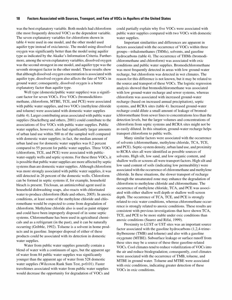
3. Quantile/quantile plot of the concentrations of 10 volatile organic compounds in oxic and anoxic conditions . . . . . . . . . . . . . . . . . . . . . . . . . . . . . . . . . . . . . . . . . . . . . . . . . . 19
iv
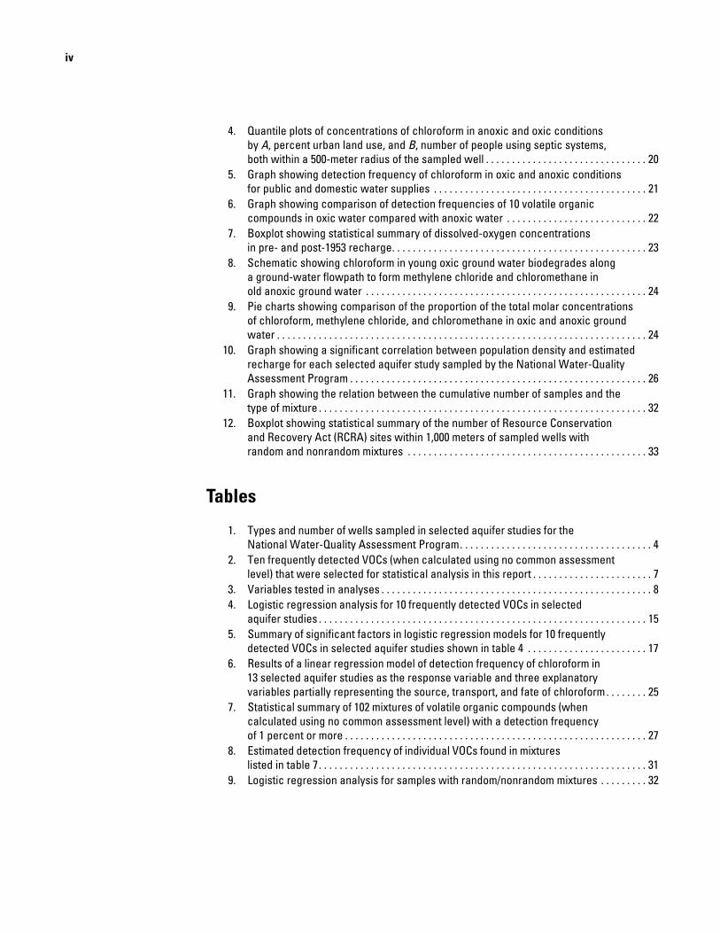
4. Quantile plots of concentrations of chloroform in anoxic and oxic conditions by A, percent urban land use, and B, number of people using septic systems, both within a 500-meter radius of the sampled well . . . . . . . . . . . . . . . . . . . . . . . . . . . . . . . 20
5. Graph showing detection frequency of chloroform in oxic and anoxic conditions for public and domestic water supplies . . . . . . . . . . . . . . . . . . . . . . . . . . . . . . . . . . . . . . . . . 21
6. Graph showing comparison of detection frequencies of 10 volatile organic compounds in oxic water compared with anoxic water . . . . . . . . . . . . . . . . . . . . . . . . . . . 22
7. Boxplot showing statistical summary of dissolved-oxygen concentrations in pre- and post-1953 recharge. . . . . . . . . . . . . . . . . . . . . . . . . . . . . . . . . . . . . . . . . . . . . . . . . 23
8. Schematic showing chloroform in young oxic ground water biodegrades along a ground-water flowpath to form methylene chloride and chloromethane in old anoxic ground water . . . . . . . . . . . . . . . . . . . . . . . . . . . . . . . . . . . . . . . . . . . . . . . . . . . . . . 24
9. Pie charts showing comparison of the proportion of the total molar concentrations of chloroform, methylene chloride, and chloromethane in oxic and anoxic ground water . . . . . . . . . . . . . . . . . . . . . . . . . . . . . . . . . . . . . . . . . . . . . . . . . . . . . . . . . . . . . . . . . . . . . . . 24
10. Graph showing a significant correlation between population density and estimated recharge for each selected aquifer study sampled by the National Water-Quality Assessment Program . . . . . . . . . . . . . . . . . . . . . . . . . . . . . . . . . . . . . . . . . . . . . . . . . . . . . . . . . 26
11. Graph showing the relation between the cumulative number of samples and the type of mixture . . . . . . . . . . . . . . . . . . . . . . . . . . . . . . . . . . . . . . . . . . . . . . . . . . . . . . . . . . . . . . . 32
12. Boxplot showing statistical summary of the number of Resource Conservation and Recovery Act (RCRA) sites within 1,000 meters of sampled wells with random and nonrandom mixtures . . . . . . . . . . . . . . . . . . . . . . . . . . . . . . . . . . . . . . . . . . . . . . 33
Tables
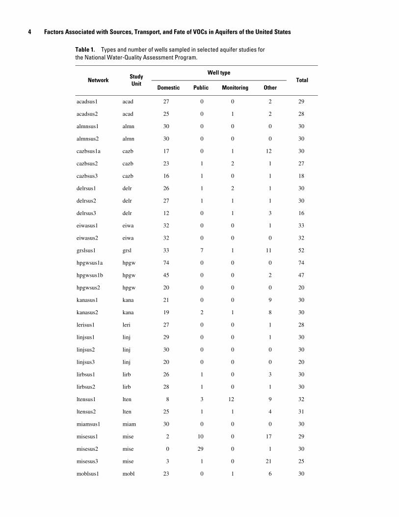
1. Types and number of wells sampled in selected aquifer studies for the National Water-Quality Assessment Program. . . . . . . . . . . . . . . . . . . . . . . . . . . . . . . . . . . . . 4
2. Ten frequently detected VOCs (when calculated using no common assessment level) that were selected for statistical analysis in this report . . . . . . . . . . . . . . . . . . . . . . . 7
3. Variables tested in analyses . . . . . . . . . . . . . . . . . . . . . . . . . . . . . . . . . . . . . . . . . . . . . . . . . . . . 84. Logistic regression analysis for 10 frequently detected VOCs in selected
aquifer studies . . . . . . . . . . . . . . . . . . . . . . . . . . . . . . . . . . . . . . . . . . . . . . . . . . . . . . . . . . . . . . . 155. Summary of significant factors in logistic regression models for 10 frequently
detected VOCs in selected aquifer studies shown in table 4 . . . . . . . . . . . . . . . . . . . . . . . 176. Results of a linear regression model of detection frequency of chloroform in
13 selected aquifer studies as the response variable and three explanatory variables partially representing the source, transport, and fate of chloroform. . . . . . . . 25
7. Statistical summary of 102 mixtures of volatile organic compounds (when calculated using no common assessment level) with a detection frequency of 1 percent or more . . . . . . . . . . . . . . . . . . . . . . . . . . . . . . . . . . . . . . . . . . . . . . . . . . . . . . . . . . 27
8. Estimated detection frequency of individual VOCs found in mixtures listed in table 7. . . . . . . . . . . . . . . . . . . . . . . . . . . . . . . . . . . . . . . . . . . . . . . . . . . . . . . . . . . . . . . 31
9. Logistic regression analysis for samples with random/nonrandom mixtures . . . . . . . . . 32
v
Conversion Factors and Abbreviations
Multiply By To obtain
cubic centimeter (cm3) 0.06102 cubic inchmeter (m) 3.281 footmillimeter (mm) 0.03937 inch
Concentrations of chemical constituents in water are given either in milligrams per liter (mg/L) or micrograms per liter (µg/L).

Factors Associated with Sources, Transport, and Fate of Volatile Organic Compounds in Aquifers of the United States and Implications for Ground-Water Management and Assessments
By Paul J. Squillace and Michael J. Moran
Abstract
Factors associated with sources, transport, and fate of volatile organic compounds (VOCs) in aquifer systems of the United States were evaluated using various statistical methods. VOC data from 1,631 wells sampled between 1996 and 2002 as part of the National Water-Quality Assessment (NAWQA) Program of the U.S. Geological Survey were used in the anal-yses. Sampled wells were randomly selected from aquifers used to supply drinking water in the regional study areas. Samples were analyzed for more than 50 VOCs from primarily domestic water supplies (1,184), followed by public-supply wells (216); the remaining wells (231) were from a variety of well types. The median well depth was 50 meters. Age-date information, avail-able from 44 percent of the sampled wells, shows that about 60 percent of the sampled water was recharged after 1953.
Ten VOCs frequently detected in aquifer samples were selected for statistical explanatory analyses and included the solvents chloromethane, methylene chloride, 1,1,1-trichloro- ethane, trichlorethene, and perchloroethene; the trihalom-ethanes bromodichloromethane and chloroform; and the gaso-line compounds toluene, 1,2,4-trimethylbenzene and methyl tert-butyl ether. Concentrations of VOCs generally were less than 1 µg/L. Source factors, in order of decreasing importance, were general land-use activity (dispersed source), septic/sewer density (dispersed source), and sites where large concentrations of VOCs are potentially released (concentrated sources), such as leaking underground storage tanks. Mixture analysis showed that 11 percent of all samples had VOC mixtures that were asso-ciated with concentrated sources; 20 percent were associated with dispersed sources. Important transport factors included well depth, screen depth, precipitation/recharge, air tempera-ture, various soil characteristics, and amount of water removed from storage during withdrawal from the aquifer. Dissolved oxygen was the explanatory factor that was strongly associated with the fate of VOCs; it proved crucial in explaining the detec-tion and concentration of many VOCs. Chloroform, for example, is more stable in water that contains oxygen. This increased stability explained the larger detection frequencies and concentrations of chloroform in water containing oxygen
compared with water having little or no oxygen. Well type (domestic or public supply) was also an important explanatory factor, but was classified as indeterminate because it was not clearly associated with the sources, transport, or fate of the VOC.
Results of multiple analyses show the importance of (1) accounting for dispersed and concentrated sources of VOCs, (2) understanding the ground-water-flow system at different scales to help explain VOC detections, (3) measuring dissolved oxygen when sampling for VOCs, and (4) limiting the type of wells sampled in monitoring networks to avoid unnecessary variance in the data.
Introduction
Ground water is used by about one-half of the population of the United States as a source of potable water, including nearly all of the 40 million or more people served by domestic water supplies (Alley and others, 1999). Concern about the quality of this heavily used resource has led to many small-scale investigations that define the risk and remediation of concen-trated sources where contaminants are released at one location. A complementary interest in dispersed sources, those where contaminants are released over large areas, has led to water-quality investigations of aquifers. Dispersed sources result from routine activity prevalent in a given setting. Discharge from septic systems, runoff from paved surfaces, and volatile organic compounds (VOCs) in air are examples of dispersed sources. Large-scale studies can provide an indication of aquifer vulner-ability and the quality of water in the aquifer as a whole, as well as identify contaminants that present the greatest risk to aqui-fers. As part of the National Water-Quality Assessment (NAWQA) Program of the U.S. Geological Survey (USGS), a plan was developed to define water-quality conditions of the most important aquifers in the Nation (Gilliom and others, 1995). The results of these aquifer studies serve as a broad-scale assessment of water quality and important issues related to aquifers.

2 Factors Associated with Sources, Transport, and Fate of VOCs in Aquifers of the United States
Part of the design of the NAWQA selected aquifer studies was extensive sampling for VOCs; that is, organic chemical compounds that have a high vapor pressure relative to their solubility in water. VOCs include components of gasoline, fuel oils, and lubricants, as well as organic solvents, fumigants, some adjuvants in pesticides, and some by-products of chlorine disinfection. VOCs can be detected virtually everywhere in the environment. They are a concern in ground water because many are mobile, persistent, and toxic. Understanding the sources, transport, and fate of VOCs is crucial for the protection and management of the ground-water resource. Because VOCs are used in numerous domestic, commercial, and industrial products and applications, they can be released to ground water through sources such as septic systems, leaking water lines and sewer lines, landfills and dumps, leaking storage tanks, and stormwater runoff.
Purpose and Scope
The purpose of this report is to (1) summarize factors affecting the sources, transport, and fate of 10 frequently detected VOCs using various statistical techniques, and (2) describe implications of the preceding for ground-water management and future ground-water assessments. The VOC data were from samples collected between 1996 and 2002 during NAWQA selected aquifer studies across the United States. The five approaches used to analyze the data were logistic regression, quantile plots, detection frequencies, network analysis, and mixture analysis.
Background and Previous Studies
Numerous household products contain VOCs (for example, toluene) and can be discharged to septic systems or disposed of improperly. In commerce and industry, VOCs are used in numerous applications, and this use results in consider-able quantities of VOCs being released to the environment (U.S. Environmental Protection Agency, 1998). Considerable amounts of gasoline are, for example, released to ground water from leaking underground storage tanks. Once in the environ-ment, VOCs can move between the atmosphere, soil, ground water, and surface water.
VOCs can be transported through the unsaturated zone in ground-water recharge, in soil vapor, or as non-aqueous-phase liquid. Any hydrologic condition that shortens residence time within the unsaturated zone can result in increased amounts of VOCs to the water table; for example, structures such as recharge basins and dry wells can accelerate transport of water and accompanying VOCs through the unsaturated zone. Furthermore, a shallow water table and abundant ground-water recharge would favor rapid transport through the unsaturated zone and increase the likelihood of VOCs reaching ground water. Some VOCs also can move slowly through the unsatur-ated zone in the gas phase and enter the top of the water table directly where concentrations partition between soil, air, and
ground water; however, this type of transport also is enhanced by the movement of recharge water (Pankow and others, 1997). For example, methyl tert-butyl ether (MTBE) is likely one of the few VOCs measured in ground water where urban air could be a source of small concentrations in shallow ground water beneath urban areas (Baehr and others, 1999; Baehr and others, 2001; Zogorski and others, in press). VOCs as non-aqueous-phase liquids could migrate to the water table by gravity without the aid of recharge or any other transport mechanism.
The transport of VOCs dissolved in ground water may be affected by sorption, advection, and dispersion. Sorption of VOCs to organic carbon in the aquifer material may slow trans-port. The effect of sorption on VOC transport is dependent on the solubility of the VOC, the amount of organic carbon in the aquifer, and the density and porosity of the aquifer. Solubility tends to be inversely related to sorption. Some very soluble VOCs like MTBE have a small sorption tendency and thus move as quickly as water does, whereas other less soluble VOCs like carbon tetrachloride (Wiedemeier and others, 1999) have a larger sorption tendency and move very slowly relative to the rate of ground-water flow. The movement of solutes by the bulk motion of flowing ground water is known as advection. The rate of advective transport varies by many orders of magni-tude in natural ground-water-flow systems (Reilly and Pollock, 1995). The tendency of solutes to spread out from the path that would be expected from advective flow is known as dispersion. Dispersion contributes to the dilution of concentrations of VOCs in ground water. VOCs can eventually be discharged with ground water into pumped wells, streams, and rivers if traveltimes are short enough or aquifer conditions are such that complete attenuation of VOCs is prevented.
The fate of any particular VOC in ground water depends largely on its persistence under the conditions present in the aquifer. VOCs that are persistent in water are more likely to be detected in ambient ground water because they can travel greater distances from their source before degradation and dilu-tion occurs. In ground water, VOCs undergo selective abiotic and biotic transformation. Hydrolysis is an example of abiotic transformation in water; for example, 1,1,1-trichloroethane (TCA) is the only commonly used chlorinated solvent that can be transformed to 1,1-dichloroethene and acetic acid by hydrol-ysis (Wiedemeier and others, 1999). Biotic transformations generally are more important than abiotic transformations for most VOCs and are linked to redox conditions in ground water. In fact, certain microorganisms under specific redox conditions can transform only some organic compounds. In redox reac-tions, inorganic electron acceptors are sequentially used in biotic transformations of organic compounds in the following order: oxygen, nitrate, manganese, iron, sulfate, and carbon dioxide. This sequential use explains why some organic compounds are persistent in an aquifer until a particular redox condition occurs; other organic compounds can be transformed under many redox conditions, but the rates can vary with the redox condition (Wiedemeier and others, 1999). Some highly chlorinated ethenes such as perchloroethene (PCE) and trichlo-roethene (TCE) also can act as electron acceptors in microbial

Methods 3
metabolism. In fact, PCE is a stronger oxidant than all of the naturally occurring inorganic electron acceptors with the excep-tion of oxygen; consequently, PCE readily undergoes reductive dechlorination (hydrogen replaces chlorine) to TCE under anaerobic conditions (Chapelle and others, 2003).
Bacteria may be unable to use VOCs as a sole source of carbon and energy when the compounds are at very small concentrations (nanograms per liter or a few micrograms per liter); this may slow the transformation of VOCs in ground water (Roch and Alexander, 1997). A decline in transformation rate with concentration may explain why some VOCs that degrade quickly for larger concentrations are commonly detected in NAWQA’s ground-water assessments at very low concentrations.
In typical technical reports and data sets, detection frequencies and concentrations are given for individual contam-inants; however, contaminants may occur more frequently as mixtures in samples than by themselves (Stackelberg and others, 2001; Squillace and others, 2002). The health implica-tion of contaminants (VOCs, pesticides, nitrate, and others) occurring together is an area of ongoing research. The challenge is to identify mixtures that present a health risk among the enor-mous number of mixtures humans are exposed to every day. The environmental importance of mixtures of contaminants is a new area of research that could help explain the sources, trans-port, and fate of VOCs.
Previous investigations have used statistical methods to show associations between land-use activity and ground-water quality for various anthropogenic contaminants. At a national scale, Kolpin and others (1998) showed an association between detection of pesticides and their use, mobility, and persistence. Nolan and others (2002) developed a logistic regression model to predict the probability of nitrate concentrations exceeding 4 milligrams per liter (mg/L) in predominantly shallow, recently recharged ground waters of the United States. The model contains factors representing fertilizer loading, percent cropland-pasture, human population density, percent well-drained soil, depth to the seasonally high water table, and pres-ence or absence of unconsolidated sand and gravel aquifers. Tesoriero and Voss (1997) used logistic regression to predict the likelihood that nitrate is present at concentrations of 3 mg/L or more in ground waters of the Puget Sound Basin in north-western Washington. Variables in this model include well depth, ground-water recharge, soil hydrologic group, surficial geology type, land-use type, and population density. Eckhardt and Stackelberg (1995) used logistic regression to predict the probability of detecting several anthropogenic contaminants in ground water beneath agricultural, suburban, and undeveloped areas of Long Island, N.Y. Two important explanatory factors were population density and land-use activity near the sampled well. Squillace and others (1999) developed a national-scale logistic regression model showing an association between the detection of any VOC and population density. Squillace and others (2004) developed logistic regression models for 14 frequently detected VOCs in the shallowest ground water beneath new residential/commercial areas in the United States. Dissolved-oxygen concentrations, estimated recharge, and land use were the most important explanatory factors for these
models. This report is a national scale assessment of associa-tions between the quality of the ground water used as a water supply and factors related to the sources, transport, and fate of VOCs.
Acknowledgments
The authors thank the many USGS personnel who collected and compiled the water-quality data used in this paper. We also thank Kerie Hitt, Barbara Ruddy, Curtis Price, and David Wolock for compiling and analyzing data using geographic information systems. Lastly, we thank Arthur Baehr, Paul Stackelberg, Gary Rowe, and John Zogorski for providing insightful reviews that substantially improved this report.
Methods
In this section, a number of methods used in this report are documented. These methods include design of NAWQA’s selected aquifer studies, sampling and analytical methods, ancillary data, statistical methods, quantile plots, and mixtures analysis.
Selected Aquifer Studies by NAWQA
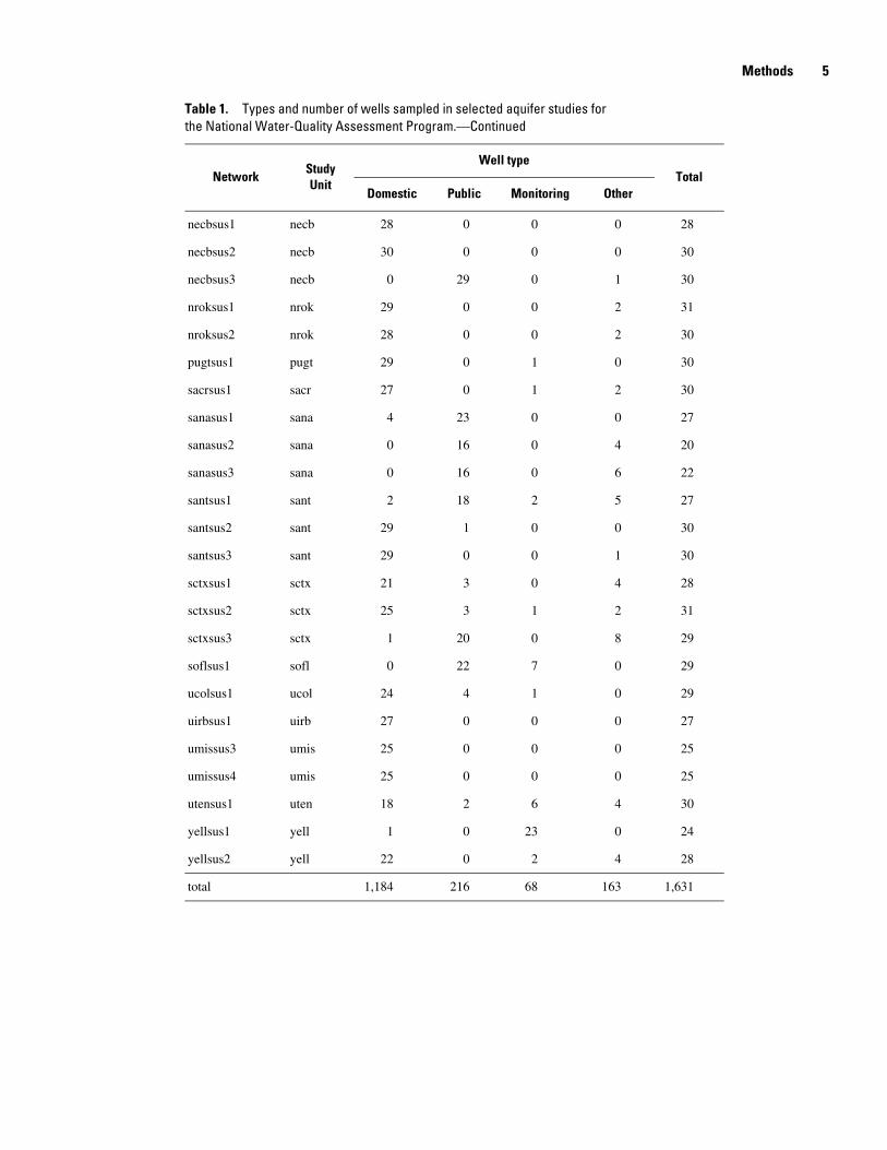
Ground-water samples from 55 selected aquifers were collected between 1996 and 2002 as part of the USGS’s NAWQA Program (fig. 1 and table 1). The selected 55 aquifer studies are a subset of the 98 aquifer studies included in the NAWQA Program’s national assessment of VOCs (Zogorski and others, in press). The original design of the NAWQA Program was to study aquifers in 60 large hydrologic basins (Gilliom and others, 1995); however, the number of hydrologic basins has been reduced to 42 (Gilliom and others, 2001). Each selected aquifer study generally contained 30 sampled wells and was done by sampling existing wells. These studies have three unique characteristics. First, samples were collected before any treatment to define the quality of water in the aquifer. Second, sampled wells were spatially distributed and randomly selected among existing wells within the targeted aquifer. Third, most of the samples were collected from domestic wells; in fact, 73 percent of the samples (1,184) were collected from domestic wells, 13 percent (216) were from public water supplies, and the remaining 14 percent (231) were from monitoring wells and a variety of other well types (table 1). Domestic wells were sampled more frequently because they were most commonly available; in addition, public-supply wells can have high pumping rates and large capture zones, which can increase the number of potential contamination sources (Stackelberg and others, 2000) compared with other types of wells. Domestic wells were also the only type of well available for sampling in many parts of the investigated aquifers. Sampling these domestic wells saved installation costs associated with monitoring wells.
4 Factors Associated with Sources, Transport, and Fate of VOCs in Aquifers of the United States
Table 1. Types and number of wells sampled in selected aquifer studies for the National Water-Quality Assessment Program.
NetworkStudyUnit
Well typeTotal
Domestic Public Monitoring Other
acadsus1 acad 27 0 0 2 29
acadsus2 acad 25 0 1 2 28
almnsus1 almn 30 0 0 0 30
almnsus2 almn 30 0 0 0 30
cazbsus1a cazb 17 0 1 12 30
cazbsus2 cazb 23 1 2 1 27
cazbsus3 cazb 16 1 0 1 18
delrsus1 delr 26 1 2 1 30
delrsus2 delr 27 1 1 1 30
delrsus3 delr 12 0 1 3 16
eiwasus1 eiwa 32 0 0 1 33
eiwasus2 eiwa 32 0 0 0 32
grslsus1 grsl 33 7 1 11 52
hpgwsus1a hpgw 74 0 0 0 74
hpgwsus1b hpgw 45 0 0 2 47
hpgwsus2 hpgw 20 0 0 0 20
kanasus1 kana 21 0 0 9 30
kanasus2 kana 19 2 1 8 30
lerisus1 leri 27 0 0 1 28
linjsus1 linj 29 0 0 1 30
linjsus2 linj 30 0 0 0 30
linjsus3 linj 20 0 0 0 20
lirbsus1 lirb 26 1 0 3 30
lirbsus2 lirb 28 1 0 1 30
ltensus1 lten 8 3 12 9 32
ltensus2 lten 25 1 1 4 31
miamsus1 miam 30 0 0 0 30
misesus1 mise 2 10 0 17 29
misesus2 mise 0 29 0 1 30
misesus3 mise 3 1 0 21 25
moblsus1 mobl 23 0 1 6 30
Methods 5
necbsus1 necb 28 0 0 0 28
necbsus2 necb 30 0 0 0 30
necbsus3 necb 0 29 0 1 30
nroksus1 nrok 29 0 0 2 31
nroksus2 nrok 28 0 0 2 30
pugtsus1 pugt 29 0 1 0 30
sacrsus1 sacr 27 0 1 2 30
sanasus1 sana 4 23 0 0 27
sanasus2 sana 0 16 0 4 20
sanasus3 sana 0 16 0 6 22
santsus1 sant 2 18 2 5 27
santsus2 sant 29 1 0 0 30
santsus3 sant 29 0 0 1 30
sctxsus1 sctx 21 3 0 4 28
sctxsus2 sctx 25 3 1 2 31
sctxsus3 sctx 1 20 0 8 29
soflsus1 sofl 0 22 7 0 29
ucolsus1 ucol 24 4 1 0 29
uirbsus1 uirb 27 0 0 0 27
umissus3 umis 25 0 0 0 25
umissus4 umis 25 0 0 0 25
utensus1 uten 18 2 6 4 30
yellsus1 yell 1 0 23 0 24
yellsus2 yell 22 0 2 4 28
total 1,184 216 68 163 1,631
Table 1. Types and number of wells sampled in selected aquifer studies for the National Water-Quality Assessment Program.—Continued
NetworkStudyUnit
Well typeTotal
Domestic Public Monitoring Other
6 Factors Associated with Sources, Transport, and Fate of VOCs in Aquifers of the United States
EXPLANATIONStudy Unit boundary with 4 letter identifierWells
PUGTPUGT
YELLYELL
SACRSACR
GRSLGRSL
SANASANA
SCTXSCTX
ACADACAD
MOBLMOBLCAZBCAZB
SOFLSOFL
SANTSANT
ALMNALMN
UMISUMIS
EIWAEIWA
UIRBUIRB
LIRBLIRB MIAMMIAM
LERILERI
DELRDELR
LINJLINJ
NECBNECB
UTENUTEN
KANAKANA
MISEMISE
UCOLUCOL
NROKNROK
LTENLTEN
PUGT
YELL
SACR
GRSL
SANA
SCTX
ACAD
MOBLCAZB
SOFL
SANT
ALMN
UMIS
EIWA
UIRB
LIRB MIAM
LERI
DELR
LINJ
NECB
UTEN
KANA
MISE
UCOL
HPGWHPGWHPGW
NROK
LTEN
GRSLGRSLGRSL
0 200 400 MILES
0 200 400 KILOMETERS
Base modified from U.S. Geological Surveydigital data, 1:2,000,000, 1990Albers Equal-Area ProjectionNorth American Datum of 1983
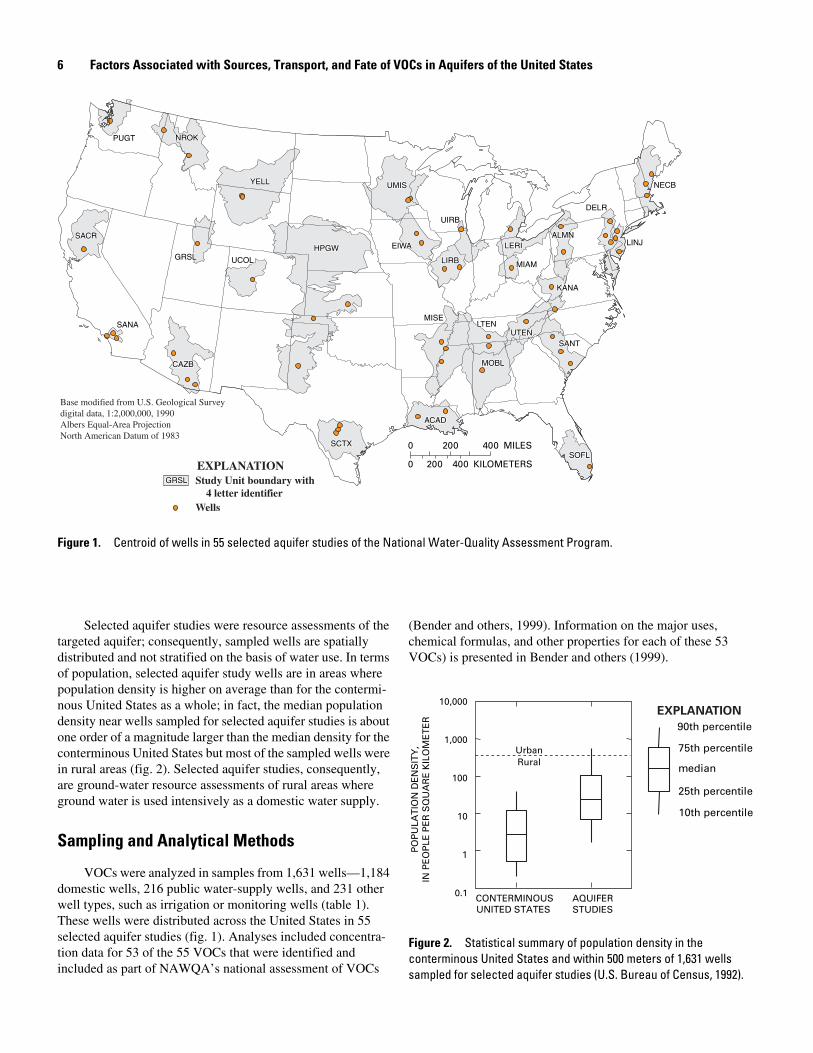
Figure 1. Centroid of wells in 55 selected aquifer studies of the National Water-Quality Assessment Program.
Selected aquifer studies were resource assessments of the targeted aquifer; consequently, sampled wells are spatially distributed and not stratified on the basis of water use. In terms of population, selected aquifer study wells are in areas where population density is higher on average than for the contermi-nous United States as a whole; in fact, the median population density near wells sampled for selected aquifer studies is about one order of a magnitude larger than the median density for the conterminous United States but most of the sampled wells were in rural areas (fig. 2). Selected aquifer studies, consequently, are ground-water resource assessments of rural areas where ground water is used intensively as a domestic water supply.
Sampling and Analytical Methods
VOCs were analyzed in samples from 1,631 wells—1,184 domestic wells, 216 public water-supply wells, and 231 other well types, such as irrigation or monitoring wells (table 1). These wells were distributed across the United States in 55 selected aquifer studies (fig. 1). Analyses included concentra-tion data for 53 of the 55 VOCs that were identified and included as part of NAWQA’s national assessment of VOCs
(Bender and others, 1999). Information on the major uses, chemical formulas, and other properties for each of these 53 VOCs) is presented in Bender and others (1999).
median
25th percentile
75th percentile
10th percentile
90th percentile
PO
PU
LAT
ION
DE
NS
ITY
,IN
PE
OP
LE P
ER
SQ
UA
RE
KIL
OM
ET
ER
10
1
0.1
100
1,000
10,000
CONTERMINOUSUNITED STATES
AQUIFERSTUDIES
RuralUrban
EXPLANATION
Figure 2. Statistical summary of population density in the conterminous United States and within 500 meters of 1,631 wells sampled for selected aquifer studies (U.S. Bureau of Census, 1992).

Methods 7
All 1,631 analyses were done at the USGS National Water Quality Laboratory in Denver, Colo., using the method that provided the lowest concentration information (method schedule 2020), currently (2005) in use at the USGS National Water Quality Laboratory (Connor and others, 1998). Although also analyzed by this low-level method, samples from Alaska and Hawaii were not included in analyses in this report because ancillary information needed for explanatory analyses was not available. Analyses were done by use of purge-and-trap, capil-lary column gas chromatography/mass spectrometry. Identifi-cation was confirmed by gas chromatographic retention time and by the resultant mass spectrum typically identified by three unique ions (Connor and others, 1998). Some of the smallest reported concentrations were estimated, indicating quantitative uncertainty. No common assessment level (for example, 0.02 or 0.2 micrograms per liter (µg/L)) was applied to any of the VOC data for this analysis. A subset of 10 VOCs listed in table 2 were frequently detected VOCs (when calculated using no common assessment level) and were selected for more detailed statistical analysis in this report. All VOC data are discussed in more detail by Moran and others (in press).
Sampling protocols and quality-assurance/quality-control plans are described by Koterba and others (1995). One primary environmental sample per well was used for the analyses in this report. Source solution blanks, equipment blanks, field blanks, trip blanks, laboratory blanks, replicate samples, and spike samples are some of the types of quality-control samples that are routinely collected. All samples were reviewed to verify the quality of the data; in particular, field blank samples were reviewed to identify any systematic contamination. If contami-nation occurred, the environmental concentration data associ-
ated with contaminated quality-control samples were not used for this analysis. There were very few incidents of systematic contamination.
Ancillary Data
Information was collected to characterize the well construction, hydrogeology, geochemistry, land use, and age of the water (table 3 and Moran and others, in press). Well depths ranged from 4 to 825 m, with a median depth of 50 m. Domestic wells had a median well depth of 45 m, and public-supply wells had a median depth of 120 m. There were 922 wells finished in unconfined aquifers and 381 wells in confined aquifers; for the remaining 328 wells, aquifer types were mixed or not identified. This information was collected because unconfined aquifers generally are considered more prone to contamination than are confined aquifers. For example, recharge water can move rela-tively quickly through sand lying above an unconfined aquifer, but recharge water moves much slower through clay lying above a confined aquifer. Dissolved-oxygen concentrations in ground water were classified as oxic or anoxic. Water was clas-sified as oxic if dissolved-oxygen concentrations were greater than 0.5 mg/L and anoxic if dissolved-oxygen concentrations were less than or equal to 0.5 mg/L. Direction of ground-water flow was not known at each sampled well. If accurate flow-direction information had been available, statistical associations between water-quality factors such as potential sources and land-use activities near the sampled well likely would have been stronger, because areas downgradient from sampled domestic wells could have been eliminated from consideration in statistical analysis.
Table 2. Ten frequently detected VOCs (when calculated using no common assessment level) that were selected for statistical analysis in this report.
[IUPAC, International Union of Pure and Applied Chemistry]
IUPAC name Selected alternative name Abbreviation VOC Group
Bromodichloromethane -- -- Trihalomethane
Trichloromethane Chloroform -- Trihalomethane
Chloromethane Methyl chloride -- Solvent
Dichloromethane Methylene chloride -- Solvent
1,1,1-Trichloroethane Methyl chloroform TCA Solvent
Trichloroethene -- TCE Solvent
Tetrachloroethene Perchloroethene PCE Solvent
Methyl-tert-butyl ether -- MTBE Gasoline oxygenate
1,2,4-Trimethylbenzene -- TMB Gasoline hydrocarbon
Methylbenzene Toluene -- Gasoline hydrocarbon
8 Factors Associated with Sources, Transport, and Fate of VOCs in Aquifers of the United States
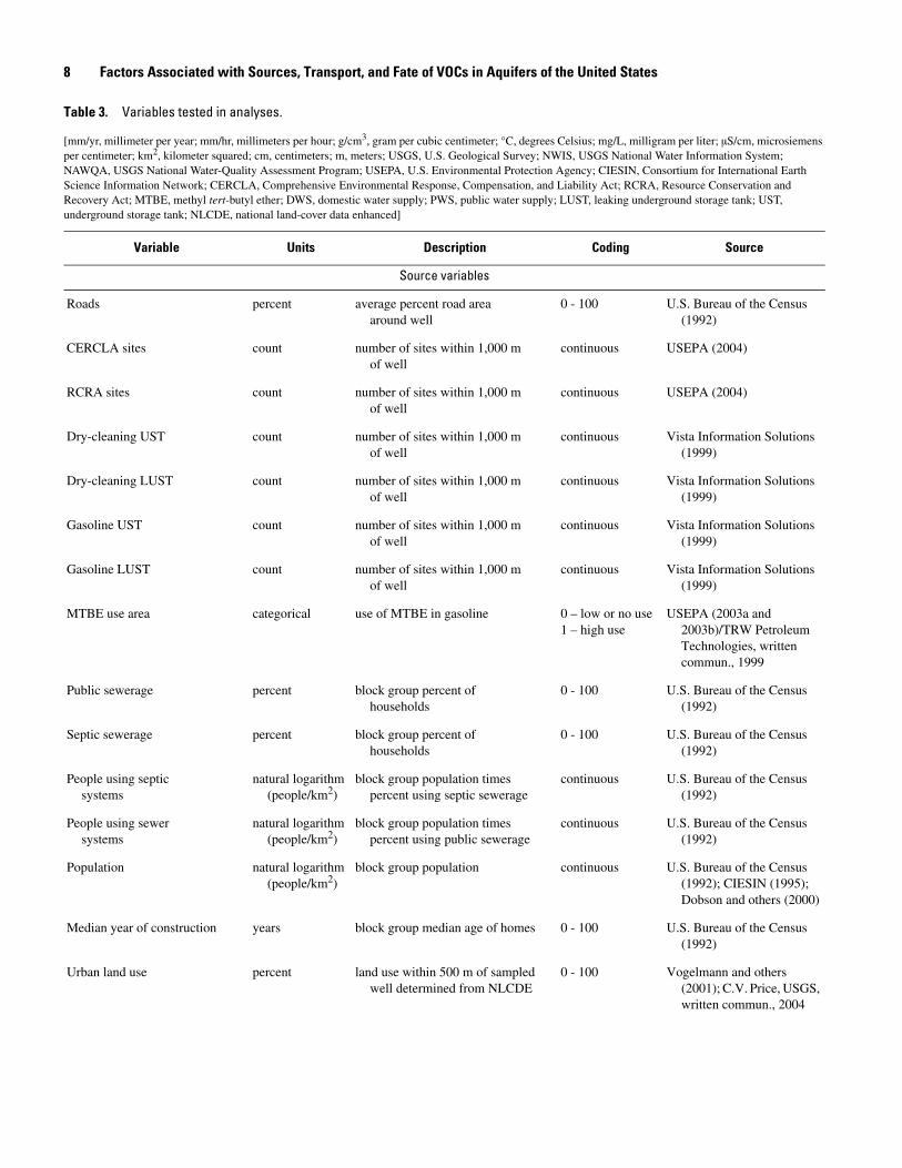
Table 3. Variables tested in analyses.
[mm/yr, millimeter per year; mm/hr, millimeters per hour; g/cm3, gram per cubic centimeter; °C, degrees Celsius; mg/L, milligram per liter; µS/cm, microsiemens per centimeter; km2, kilometer squared; cm, centimeters; m, meters; USGS, U.S. Geological Survey; NWIS, USGS National Water Information System; NAWQA, USGS National Water-Quality Assessment Program; USEPA, U.S. Environmental Protection Agency; CIESIN, Consortium for International Earth Science Information Network; CERCLA, Comprehensive Environmental Response, Compensation, and Liability Act; RCRA, Resource Conservation and Recovery Act; MTBE, methyl tert-butyl ether; DWS, domestic water supply; PWS, public water supply; LUST, leaking underground storage tank; UST, underground storage tank; NLCDE, national land-cover data enhanced]
Variable Units Description Coding Source
Source variables
Roads percent average percent road area around well
0 - 100 U.S. Bureau of the Census (1992)
CERCLA sites count number of sites within 1,000 m of well
continuous USEPA (2004)
RCRA sites count number of sites within 1,000 m of well
continuous USEPA (2004)
Dry-cleaning UST count number of sites within 1,000 m of well
continuous Vista Information Solutions (1999)
Dry-cleaning LUST count number of sites within 1,000 m of well
continuous Vista Information Solutions (1999)
Gasoline UST count number of sites within 1,000 m of well
continuous Vista Information Solutions (1999)
Gasoline LUST count number of sites within 1,000 m of well
continuous Vista Information Solutions (1999)
MTBE use area categorical use of MTBE in gasoline 0 – low or no use1 – high use
USEPA (2003a and 2003b)/TRW Petroleum Technologies, written commun., 1999
Public sewerage percent block group percent of households
0 - 100 U.S. Bureau of the Census (1992)
Septic sewerage percent block group percent of households
0 - 100 U.S. Bureau of the Census (1992)
People using septic systems
natural logarithm (people/km2)
block group population times percent using septic sewerage
continuous U.S. Bureau of the Census (1992)
People using sewer systems
natural logarithm (people/km2)
block group population times percent using public sewerage
continuous U.S. Bureau of the Census (1992)
Population natural logarithm (people/km2)
block group population continuous U.S. Bureau of the Census (1992); CIESIN (1995); Dobson and others (2000)
Median year of construction years block group median age of homes 0 - 100 U.S. Bureau of the Census (1992)
Urban land use percent land use within 500 m of sampled well determined from NLCDE
0 - 100 Vogelmann and others (2001); C.V. Price, USGS, written commun., 2004
Methods 9
Source variables—Continued
Agricultural land use percent land use within 500 m of sampled well determined from NLCDE
0 - 100 Vogelmann and others (2001); C.V. Price, USGS, written commun., 2004
Undeveloped land use percent land use within 500 m of sampled well determined from NLCDE
0 - 100 Vogelmann and others (2001); C.V. Price, USGS, written commun., (2004)
Transport variables
Public-water-supply usage percent block group percent of households
0 - 100 U.S. Bureau of the Census (1992)
Domestic-water-supply usage percent block group percent of households
0 - 100 U.S. Bureau of the Census (1992)
Households with drilled wells percent block group percent of households
0 - 100 U.S. Bureau of the Census (1992)
Households with dug wells percent block group percent of households
0 - 100 U.S. Bureau of the Census (1992)
Well casing diameter cm average casing diameter by well
continuous NWIS
Well depth m total depth of well continuous NWIS
Water level m average water level by well continuous NWIS
Depth to top of well screen m depth to the top of the screened interval in the well
continuous NWIS
Ground-water recharge mm/yr average recharge continuous Wolock (2003)
Soil permeability average mm/hr average soil permeability by soil unit
continuous Wolock (1997)
Soil permeability minimum mm/hr soil permeability of least permeable layer
continuous Wolock (1997)
Soil sand percent average soil sand content by soil unit
0 - 100 Wolock (1997)
Soil silt percent average soil silt content by soil unit
0 - 100 Wolock (1997)
Soil clay percent average soil clay content by soil unit
0 - 100 Wolock (1997)
Soil organic matter percent average organic matter content by soil unit
0 - 100 Wolock (1997)
Soil bulk density g/cm3 average bulk density of soil by soil unit
continuous Wolock (1997)
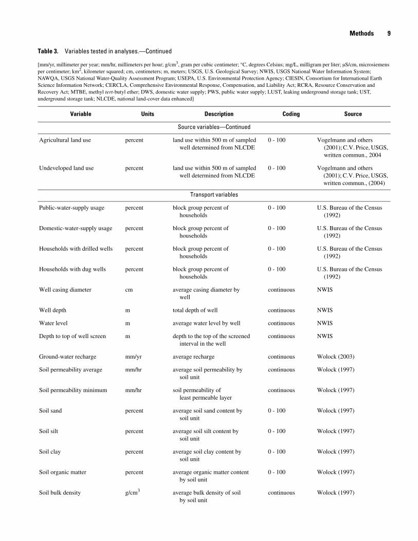
Table 3. Variables tested in analyses.—Continued
[mm/yr, millimeter per year; mm/hr, millimeters per hour; g/cm3, gram per cubic centimeter; °C, degrees Celsius; mg/L, milligram per liter; µS/cm, microsiemens per centimeter; km2, kilometer squared; cm, centimeters; m, meters; USGS, U.S. Geological Survey; NWIS, USGS National Water Information System; NAWQA, USGS National Water-Quality Assessment Program; USEPA, U.S. Environmental Protection Agency; CIESIN, Consortium for International Earth Science Information Network; CERCLA, Comprehensive Environmental Response, Compensation, and Liability Act; RCRA, Resource Conservation and Recovery Act; MTBE, methyl tert-butyl ether; DWS, domestic water supply; PWS, public water supply; LUST, leaking underground storage tank; UST, underground storage tank; NLCDE, national land-cover data enhanced]
Variable Units Description Coding Source

10 Factors Associated with Sources, Transport, and Fate of VOCs in Aquifers of the United States
Transport variables—Continued
Vertical soil permeability mm/hr average vertical soil permeability by soil unit
continuous Wolock (1997)
Hydric soils percent average percent hydric soils by soil unit
0 - 100 Wolock (1997)
Available water capacity fraction average water fraction by soil unit
0 - 1 Wolock (1997)
Slope of land surface percent average slope of land surface by soil unit
0 - 100 Wolock (1997)
Annual precipitation cm/yr average estimated annual precipitation
continuous U.S. Dept. of Commerce (1995)
Annual air temperature °C average estimated annual air temperature
continuous U.S. Dept. of Commerce (1995)
Aquifer type unitless lithologic description of the aquifer
categorical based on major lithologic units
NWIS
Aquifer confinement unitless confining condition of the aquifer
confinedmixed unconfined
NWIS
Specific conductance µS/cm average specific conductance of water in the well
continuous NWIS
Age of ground water years age of ground water at time of recharge determined by various methods
0 - older than or equal to 1953
1 - younger than 1953
NWIS
Fate variables
Temperature of ground water °C average temperature of water in the well
continuous NWIS
Dissolved oxygen (oxic/anoxic) categorical oxic water had average dissolved oxygen concentrations of water from the well greater than 0.5 mg/L; anoxic water had concentrations less than or equal to 0.5 mg/L
0 - oxic1 - anoxic
NWIS
Indeterminate variables
DWS PWS categorical major use of water from the well
0 - DWS1 - PWS
NWIS
Table 3. Variables tested in analyses.—Continued
[mm/yr, millimeter per year; mm/hr, millimeters per hour; g/cm3, gram per cubic centimeter; °C, degrees Celsius; mg/L, milligram per liter; µS/cm, microsiemens per centimeter; km2, kilometer squared; cm, centimeters; m, meters; USGS, U.S. Geological Survey; NWIS, USGS National Water Information System; NAWQA, USGS National Water-Quality Assessment Program; USEPA, U.S. Environmental Protection Agency; CIESIN, Consortium for International Earth Science Information Network; CERCLA, Comprehensive Environmental Response, Compensation, and Liability Act; RCRA, Resource Conservation and Recovery Act; MTBE, methyl tert-butyl ether; DWS, domestic water supply; PWS, public water supply; LUST, leaking underground storage tank; UST, underground storage tank; NLCDE, national land-cover data enhanced]
Variable Units Description Coding Source

Methods 11
Ancillary data on land-use activity near the sampled well was available. The limitations and assumptions associated with ancillary data are summarized here but are discussed in more detail by Moran and others (in press). Data from the U.S. Bureau of Census (1992), Vista Information Systems (1999), U.S. Department of Commerce (1995), U.S. Environmental Protection Agency (2003a and 2003b), and Wolock (1997) also were used in the analysis (table 3). Census block data from the 1990 U.S. Bureau of the Census (1992) were used to calculate the median age of homes and number of people using septic and sewer systems. Information from ancillary data was assumed to be relevant for an area within 500 m of the sampled well except for data from the U.S. Environmental Protection Agency (2004) and Vista Information Solutions (1999) where an area within 1,000 m of the sampled well was used. The percentage of people using septic and sewer systems was multiplied by popu-lation density to obtain estimates of the number of people using septic and sewer systems. Vista Information Systems data (1999) were used to calculate the densities of underground storage tanks and leaking underground storage tanks (LUST) around the sampled wells. The gasoline tanks were distin-guished from dry cleaners and other tanks by looking for a number of key words in the name of the business that would identify gasoline stations and dry cleaners. U.S. Environmental Protection Agency (2004) data were used to calculate the number of sites covered by the Comprehensive Environmental Response, Compensation, and Liability Act (CERCLA) and Resource Conservation and Recovery Act (RCRA). For each 500-m grid cell, the number of underground tanks, leaking tanks, CERCLA sites, and RCRA sites was determined using a 1,000-m circular buffer. A large circular buffer was used for these data because of the uncertainty associated with the loca-tions. Data from U.S. Environmental Protection Agency (2003a and 2003b) and TRW Petroleum Technologies (Cheryl Dickson, Bartlesville, Okla., written commun., 1999) were used to define areas that used MTBE in gasoline at concentrations greater than 3 percent by volume. The enhanced national land-cover data for 1992 (Vogelmann and others, 2001; C.V. Price, U.S. Geological Survey, written commun., 2004), which has a 30-m resolution, was used to classify the general land use in a 500-m buffer around the well. Urban land use included areas identified as low- to high-intensity residential, commercial, industrial, transportation, and urban/recreational grasses. Agricultural land use included areas identified as orchards/vine-yards, row crops, or small grains. Data were not available to show how land use changed with time.
Ancillary information was evaluated before it was used in any statistical analysis. The quality of the ancillary data was evaluated by (1) comparing the ancillary data with known locations where more detailed information was available, (2) comparing similar ancillary data sets to determine which was the most accurate, and (3) critically evaluating the ancillary data. For example, there were only three dry-cleaning LUST sites near any of the sampled wells. Using this variable in statistical analysis may produce statistically significant results, but the small number of sites is an indication that these
statistical relations are not environmentally important. A crit-ical evaluation also included, for example, cumulative distribu-tion plots that can show unusual plateaus in the data resulting from data manipulation or compilation. All these evaluations aided in understanding the strengths and weaknesses of the ancillary data.
Previous investigations provided information on estimated ground-water recharge. Ground-water recharge is an important explanatory variable because of the potential of recharge water to transport VOCs to the water table; areas with high recharge rates can have less residence time for degradation/transforma-tion within the unsaturated zone. Wolock (2003) estimated ground-water recharge indices for the United States using data from 8,249 USGS stream gages with at least 10 years of record. Assumptions required for this method are (1) aquifer storage was steady state, implying that recharge was equal to ground-water discharge; (2) recharge was discharged to streams, and (3) ground-water discharge to streams could be estimated by multi-plying a base-flow index (BFI) by long-term mean annual runoff. Stream gages on large river systems in the United States were not included in this analysis; consequently, the recharge estimates were representative of the local and possibly interme-diate ground-water-flow system. Recharge to the deep, regional ground-water-flow system probably was not reflected in the recharge estimate. The BFI was calculated at each stream gage using the Wahl and Wahl (1995) hydrograph-separation tech-nique. A grid was created from the BFI values using an inverse distance-weighting method. This grid was multiplied by a grid of average annual runoff (Wolock, 2003) to generate the average annual recharge value for the conterminous United States and to obtain point recharge estimates for the urban-land-use study wells. Irrigation may augment the transport of VOCs with ground-water recharge, but it is not known how much of this water applied to the land surface actually recharges the ground water. Evapotranspiration is largest during summer months when irrigation occurs; nevertheless, any irrigation return flow to the ground water should be reflected in the recharge index estimate. Although Wolock’s recharge estimate (Wolock, 2003) has limitations, this probably is the best recharge estimate currently (2005) available at a national scale for local and possibly intermediate ground-water-flow systems.
Thirteen selected aquifer studies were done in seven aquifers for which regional ground-water-flow models had been developed by the Regional Aquifer System Analysis (RASA) Program of the USGS (Johnston, 1999). These models did not include contaminant transport, but they can show how the hydrogeology of regional aquifers can help explain differences in water quality. RASA transient models were developed to show how factors such as withdrawal and irrigation return flow affected the transport of water within the aquifer (Johnston, 1999); however, water budgets for these large-scale models cannot be used to describe the source of water to a particular well. Ground-water withdrawal can come from three sources (Johnston, 1999): (1) decrease in storage, (2) decrease in natural discharge, and (3) induced recharge and leakage from other aquifers and recharge from irrigation return flow. An overall
12 Factors Associated with Sources, Transport, and Fate of VOCs in Aquifers of the United States
decline in water levels with time and ground-water withdrawal is an indication that water is being taken from storage. For confined aquifers, or for aquifers that have small amount of ground-water recharge, water removed from storage would likely be old water. In these situations, recharge likely occurred before anthropogenic activity began to affect ground-water quality.
Ancillary information was classified as relating to sources, transport, or fate of VOCs, with the exception of well type, which was classified as an indeterminate factor because the reason why it affects VOC detection is uncertain. For example, public water supplies have larger pumping rates, are generally deeper, and are closer to urban areas than domestic water supplies. All these factors can affect the detection of VOCs. Sources of VOCs near domestic wells can be more difficult to determine from existing ancillary data. For example, VOCs that homeowners improperly dispose of on the land surface could be a source of ground-water contamination not identified in any ancillary information.
Statistical Methods
The concentration data used in this analysis were not censored to a common assessment level because (1) the same laboratory analysis was used for all samples, (2) censoring would reduce the ability to show associations between a partic-ular VOC and explanatory factors, and (3) statistical methods like logistic regression are done for each VOC individually. Even though the lowest reported concentration for a particular VOC may change with instrument performance, the additional detections of VOCs at the smallest concentrations can be useful in establishing associations with explanatory factors. Censoring concentration data to a common assessment level is necessary when comparing, for example, detection frequencies among VOCs.
Statistics can be used for many types of analyses with water-quality data, but all of these analyses only show associa-tions and do not prove cause and effect. For example, the detec-tion of a particular VOC may be associated with increased densities of septic systems near the sampled well, but the source of the VOC could be associated with some other type of anthro-pogenic activity or factor (for example road density) that can be correlated with septic-system density.
An alpha level of 0.05 was used for all statistical analyses, which included contingency tables, Wilcoxon rank-sum test, Wilcoxon signed-rank test, Kolmogorov-Smirnov, Spearman’s rho, Pearson’s r, Wald’s t, Akaike’s Information Criteria, McFadden’s rho-squared, Hosmer/Lemeshow statistic, and log likelihood. These statistics are described in statistical books, for example, Menard (2002) and Helsel and Hirsch (1992). Contin-gency tables were used to measure the association between two nominal categorical variables if the populations of all cells were greater than or equal to five. Wilcoxon rank-sum test was used to test difference between two nominal categorical variables if a contingency table could not be used because one or more cells
had a population of less than five. The Wilcoxon signed-rank test was used to test whether matched paired values in one group were larger than those in a second group. Kolmogorov-Smirnov and Wilcoxon rank-sum tests are nonparametric tests that can be used to determine whether the distributions of two data sets are different. Spearman’s rho was calculated to deter-mine correlations between ranked concentrations in two data sets. Pearson’s r was calculated to measure the linear correlation between two data sets. Wald’s t, Akaike’s Information Criteria, McFadden’s rho-squared, Hosmer/Lemeshow statistic, and log likelihood are all statistics used to evaluate logistic regression models.
Logistic regression models were used to show associations of multiple explanatory variables (independent variables) with the presence/absence of a particular VOC (dependent variable). Models were developed for 10 frequently detected VOCs in the 1,631 samples. The presence of a VOC in this analysis is based on all reported concentrations, many of which were below health benchmarks. Explanatory factors determined at these low levels could be different than those developed at higher assessment levels. The results of these models show associa-tions only; they were not developed to be predictive models.
Using logistic regression, explanatory variables are related to the probability of occurrence of the dependent variable in a manner similar to linear regression. For this report, the depen-dent variable is binary coded as 0 or 1, with 0 indicating a non-occurrence and 1 indicating an occurrence of a particular VOC. The explanatory variables can be continuous or binary. The magnitude and sign of the estimated slope coefficient deter-mines the strength and direction of the association of a single explanatory variable with the probability of detecting a VOC in water according to the following equation:
P eβ0 β1X1 …βiXi+ +( )
1 eβ0 β1X1 …βiXi+ +( )
+--------------------------------------------------=
where
P = probability of detecting a VOC;
β0 = the y-intercept;
βi = slope coefficient of Xi explanatory variables; and
Xi = 1 to i explanatory variables.
Estimated slope coefficients with positive signs indicate an increase in the probability of detecting a VOC with an increase in the explanatory variable, whereas estimated coefficients with negative signs indicate a decrease in the probability of detecting a VOC with an increase in the explanatory variable.
For logistic regression models, unstandardized coeffi-cients were recalculated in standard deviation units so that the magnitude of the standardized coefficients could be directly compared (Menard, 2002). A standardized coefficient indicated how many standard deviations of change in the dependent
Methods 13
variable were associated with a 1-standard-deviation increase in the independent variable, as follows:
b*YX bYX( ) sX( ) R( )/slogit Y( )ˆ=
where
b*YX = the standardized logistic regression coefficient;
bYX = the unstandardized logistic regression coeffi-cient;
sX = the standard deviation of the independent vari-able X;
R = the correlation coefficient;
slogit( Y ) = the standard deviation of the logit( Y ); and
logit( Y ) = the natural logarithm of the odds ratio.
Explanatory variables were entered into the logistic regres-sion manually in a step-wise manner, and the regression was analyzed for significance at each step. For the overall regres-sion, if the likelihood ratio of the model produced a p-value of <0.05, all explanatory variables were considered significantly associated with the probability of occurrence of a VOC. The significance of nested logistic regression models was tested using the partial likelihood ratio test. For cases where one addi-tional coefficient was added, the Wald statistic was used to determine significance of the coefficient. If the Wald statistic p-value of the slope coefficient was less than 0.05 and the upper and lower bounds of the odds ratio did not include 1, the addi-tional variable was considered significantly associated with the probability of occurrence of a VOC. The significance of non-nested regression analyses was tested using Akaike’s Informa-tion Criteria (Helsel and Hirsch, 1992). The McFadden’s rho-squared can range between 0 and 1. A higher rho-squared corre-sponds to a more significant result. The Hosmer/Lemeshow statistic is a conservative test to help evaluate if the model fits the data and if the results are unduly influenced by a handful of unusual observations. The values of this statistic can range from 0 to 1 with a higher value indicating a better model.
Logistic regression models were used to look for associa-tions between ground-water quality at a particular location and current land-use activity within a circular buffer with a 500-m radius around the sampled well. No ground-water-flow analysis was done to document source of water to the sampled well. Consequently, the capture zone for the well may lie inside or outside of the 500-m radius. In these types of analyses, land use within the 500-m buffer is assumed to be representative of land use within the actual capture zone. Various conditions could adversely affect the results of this analysis, including land use within a 500-m radius that is not similar to land use within the actual capture zone of the sampled well, available land-use data that are not sufficiently accurate, prior land-use activity that has
affected water quality, current land-use activity that has not had time to affect shallow ground water, only small areas within the 500-m buffer that affect water quality, and concentrated sources that could be sufficiently spread out to give the appearance of dispersed sources. Spurious associations can result if VOCs were formed by the degradation of other VOCs, if the VOCs occur naturally (for example, chloroform (Laturnus and others, 2002)), or if sources have not been included in the model. In these situations, however, model diagnostics usually indicate problems with the explanatory factors. In spite of these potential problems, several previous studies have shown a relation between land use and water quality (Eckhardt and Stackelberg, 1995; Grady and Mullaney, 1998; Nolan and Stoner, 2000, Barbash and others, 2001; Robinson, 2002).
For each VOC, various logistic regression models are possible, but information from a variety of statistical measures were used to select the final model (log likelihood, Wald’s t, Akaike’s Information Criteria, McFadden’s rho-squared, Hosmer/Lemeshow statistic) (Helsel and Hirsch, 1992; Menard, 2002). These models all had explanatory variables with a Wald’s t p-value of <0.05. The negative log likelihood was minimized, and nonnested models were compared by use of Akaike’s Information Criteria. Models with a large McFadden’s rho-squared were selected over those with lower values; and, when possible, models with a high Hosmer/Leme-show statistic were selected over those with lower values to ensure that the model was not unduly affected by a small number of unusual observations. Although a variety of statis-tical measures were used to evaluate the many possible models, these models should not be viewed as definitive, unique, or suit-able for predictive purposes. These models may change as more detailed ancillary or ground-water-flow information becomes available; nevertheless, some general conclusions can be drawn from the results of these initial models.
Quantile Plots
Quantile plots were used to show the distribution of the sample data. The quantile of a sample is the data point corre-sponding to a given fraction of the data at or less than a partic-ular concentration (Helsel and Hirsch, 1992). A quantile plot looks like a cumulative sample distribution function. The spread, skewness, and other characteristics of all the data could be examined in these plots; furthermore, more of the data can be displayed in quantile plots than in boxplots. The quantile plots shown in this report start at the fraction of data with a measured concentration. Direct comparisons between concentration distributions in two data sets also were displayed by graphing the quantiles of one data set in relation to the second in quantile/quantile plots (Helsel and Hirsch, 1992).
14 Factors Associated with Sources, Transport, and Fate of VOCs in Aquifers of the United States
Mixture Analysis
A mixture is defined as a unique combination of two or more particular compounds, regardless of the presence of other compounds that may occur in the same sample (Squillace and others, 2002). Thus, a sample with three detected compounds (A, B, and C) contains four different mixtures (AB, AC, BC, and ABC). This approach is most useful if VOCs in a single sample originate from different sources or some are degradation products. The number of mixtures within a data set can be very large, and samples with the largest numbers of compounds yield most of the mixtures.
The theoretical probability of one VOC occurring with a second VOC is equal to the product of the individual detection frequencies of each VOC, if the detections are independent. For example, the theoretical probability of compound A occurring with compound B in a single sample is equal to the detection frequency of A multiplied by the detection frequency of B. Independence means that the detection of one VOC does not affect the probability of finding a second VOC; however, there are at least three reasons why independence is usually not achieved. First, areas of an aquifer that are most transmissive also are areas where VOCs are most likely to be detected, given a uniform contaminant load at the land surface. Second, VOCs can be transformed from one VOC to a second, resulting in a mixture of the parent compound and the transformation product. Third, VOCs that share a common source are more likely to be detected together in ground water.
The ratio of the actual detection frequency to the theoret-ical probability of detecting a mixture, called the detection frequency ratio (DFR), can be used to show associations with possible sources. If a mixture had a DFR close to 1, then the frequency of these VOCs occurring together can be explained by chance and, consequently, random co-occurrence of VOCs. The DFR can be somewhat larger than 1 for some random mixtures if there are variations in aquifer vulnerability given a uniform contaminant load. In vulnerable parts of the aquifer, many of the potential VOC contaminants reach the ground water because transport of all VOCs to the water table is quick, with little degradation. In less vulnerable parts of the aquifer, only the more mobile and persistent VOCs reach the ground water. If a mixture had a DFR much greater than 1, then the frequency of these VOCs occurring together cannot be explained by chance; consequently, nonrandom co-occurrence of VOCs is implied. These nonrandom mixtures could be derived from, for example, leaking underground storage tanks. The DFR also could be large for some mixtures if one VOC is transformed to a second and they both occur together in one sample. Possible transformation products, however, can some-times be identified, especially if redox conditions favor the degradation of the parent compound.
Analysis of the Sources, Transport, and Fate of VOCs
In this section, the analysis of the sources, transport, and fate of VOCs is presented using various methods. These methods include logistic regression, quantile plots, detection frequency, network analysis, and the use of mixtures.
Logistic Regression to Determine Significant Associations
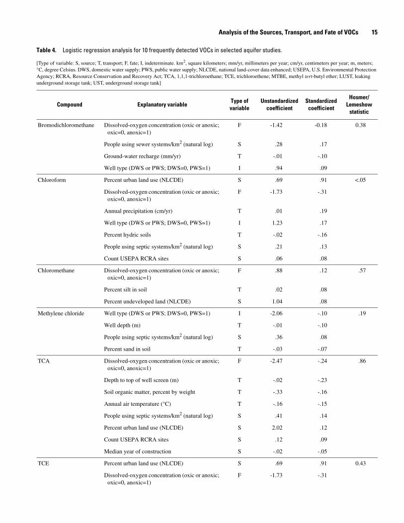
Logistic regression was used to determine associations between the occurrence of 10 frequently detected VOCs and explanatory factors related to their sources, transport, and fate (table 4). The advantage of this method is that it is multivariate and, if the coefficients are standardized, the relative importance of the factors in the model can be determined. A general discus-sion of factors associated with the 10 VOCs is followed by factors associated with groups of VOCs.
A summary of significant factors or groups of factors asso-ciated with sources, transport, and fate for all 10 VOCs is given in table 5. Important source factors include MTBE use areas, RCRA sites, LUST sites, underground storage tank (UST) sites, septic systems, sewer systems, and general land-use character-istics such as the amount of urban land. The relative importance of each of these factors varies by individual VOC, but RCRA, LUST, and UST sites were typically not as important as factors that describe general land-use characteristics. Important trans-port factors include well depth, screen depth, precipitation, ground-water recharge, air temperature, and various soil char-acteristics. The deeper wells had a smaller chance of VOC detection. Generally, more precipitation or ground-water recharge resulted in more VOC detections. Colder temperatures were associated with increased detection of some VOCs because volatility and biodegradation is reduced with cold temperatures, increasing the possibility of VOCs entering the ground water. Only one factor—dissolved-oxygen concentra-tion—was associated with the fate of VOCs. This factor was significant for 8 of the 10 VOCs investigated and was the first or second most important factor for 6 VOCs. Only chlo-romethane was associated with anoxic conditions; detections of the other seven VOCs were associated with oxic conditions.
Analysis of the Sources, Transport, and Fate of VOCs 15
Table 4. Logistic regression analysis for 10 frequently detected VOCs in selected aquifer studies.
[Type of variable: S, source; T, transport; F, fate; I, indeterminate. km2, square kilometers; mm/yr, millimeters per year; cm/yr, centimeters per year; m, meters; °C, degree Celsius. DWS, domestic water supply; PWS, public water supply; NLCDE, national land-cover data enhanced; USEPA, U.S. Environmental Protection Agency; RCRA, Resource Conservation and Recovery Act; TCA, 1,1,1-trichloroethane; TCE, trichloroethene; MTBE, methyl tert-butyl ether; LUST, leaking underground storage tank; UST, underground storage tank]
Compound Explanatory variableType of variable
Unstandardized coefficient
Standardized coefficient
Hosmer/Lemeshow
statistic
Bromodichloromethane Dissolved-oxygen concentration (oxic or anoxic; oxic=0, anoxic=1)
F -1.42 -0.18 0.38
People using sewer systems/km2 (natural log) S .28 .17
Ground-water recharge (mm/yr) T -.01 -.10
Well type (DWS or PWS; DWS=0, PWS=1) I .94 .09
Chloroform Percent urban land use (NLCDE) S .69 .91 <.05
Dissolved-oxygen concentration (oxic or anoxic; oxic=0, anoxic=1)
F -1.73 -.31
Annual precipitation (cm/yr) T .01 .19
Well type (DWS or PWS; DWS=0, PWS=1) I 1.23 .17
Percent hydric soils T -.02 -.16
People using septic systems/km2 (natural log) S .21 .13
Count USEPA RCRA sites S .06 .08
Chloromethane Dissolved-oxygen concentration (oxic or anoxic; oxic=0, anoxic=1)
F .88 .12 .57
Percent silt in soil T .02 .08
Percent undeveloped land (NLCDE) S 1.04 .08
Methylene chloride Well type (DWS or PWS; DWS=0, PWS=1) I -2.06 -.10 .19
Well depth (m) T -.01 -.10
People using septic systems/km2 (natural log) S .36 .08
Percent sand in soil T -.03 -.07
TCA Dissolved-oxygen concentration (oxic or anoxic; oxic=0, anoxic=1)
F -2.47 -.24 .86
Depth to top of well screen (m) T -.02 -.23
Soil organic matter, percent by weight T -.33 -.16
Annual air temperature (°C) T -.16 -.15
People using septic systems/km2 (natural log) S .41 .14
Percent urban land use (NLCDE) S 2.02 .12
Count USEPA RCRA sites S .12 .09
Median year of construction S -.02 -.05
TCE Percent urban land use (NLCDE) S .69 .91 0.43
Dissolved-oxygen concentration (oxic or anoxic; oxic=0, anoxic=1)
F -1.73 -.31

16 Factors Associated with Sources, Transport, and Fate of VOCs in Aquifers of the United States
TCE—Continued Annual precipitation (cm/yr) T 0.01 0.19
Well type (DWS or PWS; DWS=0, PWS=1) I 1.23 .17
Percent hydric soils T -.02 -.16
People using septic systems/km2 (natural log) S .21 .13
Count USEPA RCRA sites S .06 .08
PCE Depth to top of well screen (m) T -0.01 -0.21 .34
Dissolved-oxygen concentration (oxic or anoxic; oxic=0, anoxic=1)
F -.99 -.18
Well type (DWS or PWS; DWS=0, PWS=1) I 1.04 .15
Percent urban land use (NLCDE) S 1.40 .15
People using septic systems/km2 (natural log) S .15 .09
Count USEPA RCRA sites S .04 .06
MTBE Annual precipitation (cm/yr) T .03 .27 .48
MTBE use area S 2.36 .26
Depth to top of well screen (m) T -.02 -.26
Well type (DWS or PWS; DWS=0, PWS=1) I 1.97 .20
Annual air temperature (°C) T -.12 -.15
Dissolved-oxygen concentration (oxic or anoxic; oxic=0, anoxic=1)
F -.83 -.11
Count gasoline LUST sites S .49 .10
1,2,4-Trimethylbenzene People using septic systems/km2 (natural log) S -.28 -.17 .07
Annual air temperature (°C) T -.06 -.11
Annual precipitation (cm/yr) T -.01 -.08
Count gasoline UST sites S .20 .07
Toluene Annual air temperature (°C) T -.08 -.13 .22
Median year of construction S -.03 -.10
Count gasoline LUST sites S .41 .10
Well type (DWS or PWS; DWS=0, PWS=1) I -.86 -.10
Dissolved-oxygen concentration (oxic or anoxic; oxic=0, anoxic=1)
F -.49 -.08
Percent hydric soils T .01 .08
Table 4. Logistic regression analysis for 10 frequently detected VOCs in selected aquifer studies.—Continued
[Type of variable: S, source; T, transport; F, fate; I, indeterminate. km2, square kilometers; mm/yr, millimeters per year; cm/yr, centimeters per year; m, meters; °C, degree Celsius. DWS, domestic water supply; PWS, public water supply; NLCDE, national land-cover data enhanced; USEPA, U.S. Environmental Protection Agency; RCRA, Resource Conservation and Recovery Act; TCA, 1,1,1-trichloroethane; TCE, trichloroethene; MTBE, methyl tert-butyl ether; LUST, leaking underground storage tank; UST, underground storage tank]
Compound Explanatory variableType of variable
Unstandardized coefficient
Standardized coefficient
Hosmer/Lemeshow
statistic
Analysis of the Sources, Transport, and Fate of VOCs 17
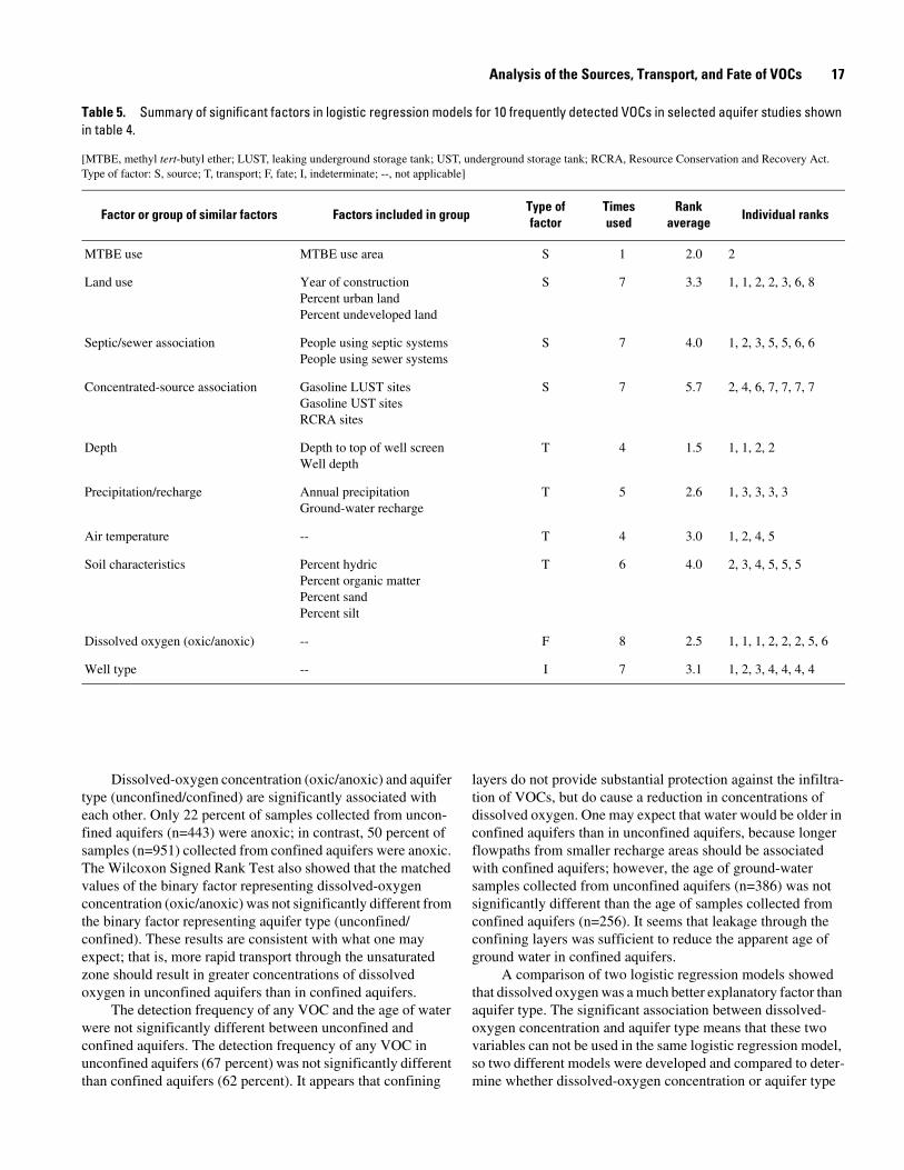
Table 5. Summary of significant factors in logistic regression models for 10 frequently detected VOCs in selected aquifer studies shown in table 4.
[MTBE, methyl tert-butyl ether; LUST, leaking underground storage tank; UST, underground storage tank; RCRA, Resource Conservation and Recovery Act. Type of factor: S, source; T, transport; F, fate; I, indeterminate; --, not applicable]
Factor or group of similar factors Factors included in groupType offactor
Times used
Rank average
Individual ranks
MTBE use MTBE use area S 1 2.0 2
Land use Year of constructionPercent urban landPercent undeveloped land
S 7 3.3 1, 1, 2, 2, 3, 6, 8
Septic/sewer association People using septic systemsPeople using sewer systems
S 7 4.0 1, 2, 3, 5, 5, 6, 6
Concentrated-source association Gasoline LUST sitesGasoline UST sitesRCRA sites
S 7 5.7 2, 4, 6, 7, 7, 7, 7
Depth Depth to top of well screenWell depth
T 4 1.5 1, 1, 2, 2
Precipitation/recharge Annual precipitationGround-water recharge
T 5 2.6 1, 3, 3, 3, 3
Air temperature -- T 4 3.0 1, 2, 4, 5
Soil characteristics Percent hydricPercent organic matterPercent sandPercent silt
T 6 4.0 2, 3, 4, 5, 5, 5
Dissolved oxygen (oxic/anoxic) -- F 8 2.5 1, 1, 1, 2, 2, 2, 5, 6
Well type -- I 7 3.1 1, 2, 3, 4, 4, 4, 4
Dissolved-oxygen concentration (oxic/anoxic) and aquifer type (unconfined/confined) are significantly associated with each other. Only 22 percent of samples collected from uncon-fined aquifers (n=443) were anoxic; in contrast, 50 percent of samples (n=951) collected from confined aquifers were anoxic. The Wilcoxon Signed Rank Test also showed that the matched values of the binary factor representing dissolved-oxygen concentration (oxic/anoxic) was not significantly different from the binary factor representing aquifer type (unconfined/confined). These results are consistent with what one may expect; that is, more rapid transport through the unsaturated zone should result in greater concentrations of dissolved oxygen in unconfined aquifers than in confined aquifers.
The detection frequency of any VOC and the age of water were not significantly different between unconfined and confined aquifers. The detection frequency of any VOC in unconfined aquifers (67 percent) was not significantly different than confined aquifers (62 percent). It appears that confining
layers do not provide substantial protection against the infiltra-tion of VOCs, but do cause a reduction in concentrations of dissolved oxygen. One may expect that water would be older in confined aquifers than in unconfined aquifers, because longer flowpaths from smaller recharge areas should be associated with confined aquifers; however, the age of ground-water samples collected from unconfined aquifers (n=386) was not significantly different than the age of samples collected from confined aquifers (n=256). It seems that leakage through the confining layers was sufficient to reduce the apparent age of ground water in confined aquifers.
A comparison of two logistic regression models showed that dissolved oxygen was a much better explanatory factor than aquifer type. The significant association between dissolved-oxygen concentration and aquifer type means that these two variables can not be used in the same logistic regression model, so two different models were developed and compared to deter-mine whether dissolved-oxygen concentration or aquifer type
18 Factors Associated with Sources, Transport, and Fate of VOCs in Aquifers of the United States
was the best explanatory variable. Both models had chloroform (the most frequently detected VOC) as the dependent variable. The seven explanatory variables for chloroform shown in table 4 were used in one model, and the other model used aquifer type instead of oxic/anoxic. The model using dissolved oxygen was significantly better than the model using aquifer type as indicated by the Akaike’s Information Criteria. Further-more, among the seven explanatory variables, dissolved oxygen was the second strongest in one model, and aquifer type was the seventh strongest factor in the other model. These results show that although dissolved-oxygen concentration is associated with aquifer type, dissolved oxygen also affects the fate of VOCs in ground water; consequently, dissolved oxygen is a better explanatory factor than aquifer type.
Well type (domestic/public water supplies) was a signifi-cant factor for seven VOCs. Five VOCs (bromodichloro- methane, chloroform, MTBE, TCE, and PCE) were associated with public water supplies, and two VOCs (methylene chloride and toluene) were associated with domestic water supplies (table 4). Larger contributing areas associated with public water supplies (Stackelberg and others, 2001) could contribute to the associations of five VOCs with public water supplies. Public water supplies, however, also had significantly larger amounts of urban land use within 500 m of the sampled well compared with domestic water supplies; in fact, the median amount of urban land use for domestic water supplies was 0.2 percent compared to 55 percent for public water supplies. Three VOCs (chloroform, TCE, and PCE) were associated with public-water-supply wells and septic systems. For these three VOCs, it is possible that public water supplies are more affected by septic systems than are domestic water supplies. Although chloroform was more strongly associated with public water supplies, it was still detected in 26 percent of the domestic wells. Chloroform can be formed in septic systems if, for example, household bleach is present. Triclosan, an antimicrobial agent used in household dishwashing soaps, also reacts with chlorinated water to produce chloroform (Rule and others, 2005). In anoxic conditions, at least some of the methylene chloride and chlo-romethane would be expected to come from degradation of chloroform. Methylene chloride also is used as paint stripper and could have been improperly disposed of in some septic systems. Chloromethane has been used in agricultural chemi-cals and as a refrigerant (in the past), and it can be naturally occurring (Gribble, 1992). Toluene is a solvent in home prod-ucts and in gasoline. Improper disposal of either of these products could be associated with its detection in domestic water supplies.
Water from public water supplies generally contain a blend of water with a continuum of ages, but the apparent age of water from 84 public water supplies was significantly younger than the apparent age of water from 528 domestic water supplies (Wilcoxon Rank Sum Test, p<0.01). Faster traveltimes associated with water from public water supplies would decrease the opportunity for degradation of VOCs and
could partially explain why five VOCs were associated with public water supplies compared with two VOCs with domestic water supplies.
Important similarities and differences are apparent in factors associated with the occurrence of VOCs within three groups—trihalomethanes (THMs), solvents, and gasoline hydrocarbons (table 4). The occurrence of THMs (bromodi- chloromethane and chloroform) was associated with oxic conditions and public water supplies. Bromodichloromethane was most frequently detected in areas with low ground-water recharge, but chloroform was detected in wet climates. The reason for this difference is not known, but it may be related to the source and transport of these VOCs. The logistic regression analysis showed that bromodichloromethane was associated with low ground-water recharge and sewer systems, whereas chloroform was associated with increased ground-water recharge (based on increased annual precipitation), septic systems, and RCRA sites (table 4). Increased ground-water recharge could dilute a small amount of leakage of bromod-ichloromethane from sewer lines to concentrations less than the detection levels, but the larger volumes and concentrations of chloroform from septic systems and RCRA sites might not be as easily diluted. In this situation, ground-water recharge helps transport chloroform to public wells.
Many similar factors were associated with the occurrence of solvents (chloromethane, methylene chloride, TCA, TCE, and PCE). Septic-system density, urban land use, and proximity to RCRA sites all were identified as possible sources of solvents. High silt, low sand, and low organic content, and shallow wells or screens all were transport factors. High silt and low sand content of soils (indicating low permeability) were associated with the occurrence of chloromethane and methylene chloride. In these situations, the slower transport of recharge through the unsaturated zone may enhance the degradation of chloroform to methylene chloride and chloromethane. The occurrence of methylene chloride, TCA, and PCE was associ-ated with either shallow well depth or shallow well-screen depth. The occurrence of TCA, TCE, and PCE is strongly related to oxic water conditions, whereas chloromethane occur-rence is strongly related to anoxic conditions. These results are consistent with previous investigations that have shown TCA, TCE, and PCE to be more stable under oxic conditions than anoxic conditions (Suarez and Rifai, 1999).
Proximity to LUST or UST sites was an important source factor associated with the gasoline hydrocarbons (1,2,4-trime-thylbenzene (TMB) and toluene) and also with a gasoline oxygenate (MTBE). Subsurface leakage or surface runoff from these sites may be a source of these three gasoline-related VOCs. Cool climates tend to reduce volatilization of VOCs into the air and reduce biodegradation; consequently, cool climates were associated with the occurrence of TMB, toluene, and MTBE in ground water. Toluene and MTBE were associated with oxic conditions, indicating greater detection of these VOCs in oxic conditions.
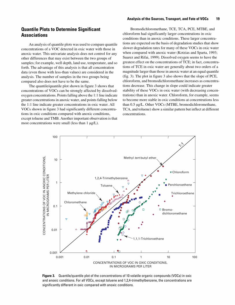
Analysis of the Sources, Transport, and Fate of VOCs 19
Quantile Plots to Determine Significant Associations
An analysis of quantile plots was used to compare quantile concentrations of a VOC detected in oxic water with those in anoxic water. This univariate analysis does not control for any other differences that may exist between the two groups of samples; for example, well depth, land use, temperature, and so forth. The advantage of this analysis is that all concentration data (even those with less-than values) are considered in the analysis. The number of samples in the two groups being compared also does not have to be the same.
The quantile/quantile plot shown in figure 3 shows that concentrations of VOCs can be strongly affected by dissolved-oxygen concentrations. Points falling above the 1:1 line indicate greater concentrations in anoxic water, and points falling below the 1:1 line indicate greater concentrations in oxic water. All VOCs shown in figure 3 had significantly different concentra-tions in oxic conditions compared with anoxic conditions, except toluene and TMB. Another important observation is that most concentrations were small (less than 1 µg/L).
Bromodichloromethane, TCE, TCA, PCE, MTBE, and chloroform had significantly larger concentrations in oxic conditions than in anoxic conditions. These larger concentra-tions are expected on the basis of degradation studies that show slower degradation rates for many of these VOCs in oxic water when compared with anoxic water (Kotzias and Sparta, 1993; Suarez and Rifai, 1999). Dissolved oxygen seems to have the greatest effect on the concentrations of TCE; in fact, concentra-tions of TCE in oxic water are generally about two orders of a magnitude larger than those in anoxic water at an equal quantile (fig. 3). The plot in figure 3 also shows that the slope of PCE, chloroform, and bromodichloromethane increases as concentra-tions decrease. This change in slope could indicate greater stability of these VOCs in oxic water (with decreasing concen-trations) than in anoxic water. Chloroform, for example, seems to become more stable in oxic conditions at concentrations less than 0.5 µg/L. Other VOCs (MTBE, bromodichloromethane, TCA, and toluene) show a similar pattern but inflect at different concentrations.
Chloromethane
Methylene chloride Trichloroethene
Perchloroethene
Methyl tert-butyl ether
Chloroform
1:1
1,2,4-Trimethybenzene
Toluene
Bromo-dichloromethane
1,1,1-Trichloroethane
CO
NC
EN
TR
AT
ION
S O
F V
OC
IN A
NO
XIC
CO
ND
ITIO
NS
,IN
MIC
RO
GR
AM
S P
ER
LIT
ER
CONCENTRATIONS OF VOC IN OXIC CONDITIONS,IN MICROGRAMS PER LITER
100
10
1
0.1
0.01
0.0010.001 0.01 0.1 1 10 100
Figure 3. Quantile/quantile plot of the concentrations of 10 volatile organic compounds (VOCs) in oxic and anoxic conditions. For all VOCs, except toluene and 1,2,4-trimethylbenzene, the concentrations are significantly different in oxic compared with anoxic conditions.

20 Factors Associated with Sources, Transport, and Fate of VOCs in Aquifers of the United States
The concentrations of chloromethane, methylene chloride, toluene, and TMB were larger in anoxic conditions than in oxic conditions; however, only chloromethane and methylene chlo-ride had significantly larger concentrations in anoxic condi-tions. If chloromethane and methylene chloride originate primarily from the degradation of chloroform in anoxic water (Norris and others, 1994), then finding larger concentrations of these two VOCs in anoxic water would be expected. Gasoline hydrocarbons such as toluene and TMB are known to be more stable in anoxic conditions than in oxic conditions (Suarez and Rifai, 1999); however, the concentrations detected in this study generally were less than 1 µg/L. At these concentrations, degra-dation rates may slow considerably (Roch and Alexander, 1997) and may become similar to those in oxic conditions.
The quantile plots in figure 4 show that concentrations of chloroform are more strongly affected by the amount of urban land use and people using septic systems in oxic conditions than in anoxic conditions. Data for figure 4A were divided into four groups on the basis of dissolved-oxygen concentrations and the amount of urban land use. Data for figure 4B were also divided into four groups on the basis of dissolved-oxygen concentra-tions and the number of people using septic systems near the sampled well—about 75 percent of the sampled wells had less than 40 people using septic systems within 500 m of the sampled well, and 25 percent had 40 or more people using septic systems. Figures 4A and 4B show that the concentrations of chloroform were less in anoxic conditions than oxic condi-tions. These results are consistent with data shown in figure 3; however, figures 4A and 4B also show that anthropogenic activity had a greater affect on the concentrations of chloroform
in oxic conditions than in anoxic conditions. In anoxic condi-tions, the amount of urban land use had no effect on the concen-trations of chloroform, and the number of people using septic systems had only minimal effect on the concentrations of chloroform. In oxic conditions, the amount of urban land use and the number of people using septic systems had a dramatic effect on the concentrations of chloroform (fig. 4A). These results generally are substantiated by Spearman’s correlation analysis. In oxic conditions, there was a significant correlation between chloroform concentrations and (1) urban land use and (2) people using septic systems. In anoxic conditions, chloro-form concentrations were not correlated with urban land use but were correlated with the number of people using septic systems.
Detection Frequency to Determine Significant Associations
Detection frequencies can be used as a simple statistical analysis to help understand the sources, transport, and fate of VOCs. Detection frequencies can be calculated using all the data; alternatively, the data can be divided into two or more groups on the basis of a single variable. A contingency table using the Pearson’s chi square test can be used to determine if significant differences exist between the groups of data. This statistical method is easy to do, results are easy to understand, and all data (even those with values less than the reporting level) are included in the analysis; however, the disadvantage is that subdividing the data into groups can result in small numbers of samples in each group.
Urban land use, in percent People using septic systems
CONCENTRATION OF CHLOROFORM,IN MICROGRAMS PER LITER
0.001 0.01 0.1 1 10
FRA
CT
ION
OF
DA
TA
CONCENTRATION OF CHLOROFORM,IN MICROGRAMS PER LITER
1.0
0.9
0.8
0.6
0.7
0.5
0.4
0.3
0.2
0.1
0
FRA
CT
ION
OF
DA
TA
1.0
0.9
0.8
0.6
0.7
0.5
0.4
0.3
0.2
0.1
00.001 0.01 0.1 1 10
Less than 40Greater than or equal to 40
Less than 40Greater than or equal to 40
Anoxic conditions
Oxic conditionsLess than 50Greater than or equal to 50
Less than 50Greater than or equal to 50
Anoxic conditions
Oxic conditions
BA
Figure 4. Quantile plots of concentrations of chloroform in anoxic and oxic conditions by A, percent urban land use, and B, number of people using septic systems, both within a 500-meter radius of the sampled well.

Analysis of the Sources, Transport, and Fate of VOCs 21
Confining layers are thought to provide some protection to ground water from anthropogenic contamination because of the slow movement of water through the confining layer. To test this hypothesis, paired detection frequencies of the 10 VOCs listed in table 2 were compared between aquifers that were classified as confined or unconfined. Using the Wilcoxon signed rank, there was no statistically significant difference in the detection frequencies of these 10 VOCs in the two types of aquifers. Results indicate that either the data or method used to classify aquifers into groups was not sufficiently accurate to identify aquifers less susceptible to contamination or that confining units in general do not protect ground water from VOC contamination.
Domestic and public water supplies had larger detection frequency of chloroform in oxic water compared with anoxic water (fig. 5), when detection frequencies were calculated using no common assessment level. For public-supply wells, there was a significant difference in chloroform detection frequency in oxic conditions (81 percent) compared with anoxic condi-tions (13 percent). For domestic supply wells, there also was a significant difference in chloroform detection frequency in oxic conditions (31 percent) compared with anoxic conditions (12 percent). These differences demonstrate the importance of dissolved-oxygen concentrations but also illustrate the impor-tance of well type. There was, however, no significant differ-ence in detection frequencies of chloroform between domestic and public water supplies with anoxic water.
A comparison of the detection frequencies of 10 VOCs in oxic and anoxic ground water is shown in figure 6. Again,
detection frequencies were calculated using no common assess-ment level. Detection frequencies for all VOCs are significantly different in these two oxygen conditions, except those for TMB and toluene. Those VOCs above the 1:1 line were more frequently detected in anoxic conditions than in oxic conditions, and VOCs below the 1:1 line were more frequently detected in oxic conditions than in anoxic conditions. Differences in detec-tion frequencies are generally consistent with published rates of biodegradation (Suarez and Rifai, 1999). For example, chloro-form, PCE, TCE, and TCA are more persistent in oxic ground water, which was confirmed by their higher detection frequency in oxic ground water than in anoxic ground water (fig. 6). Toluene is more stable in anoxic water (Suarez and Rifai, 1999) but was detected more frequently in oxic conditions; however, this was not a statistically significant difference. The remaining VOCs have very few published degradation rates; conse-quently, it is impossible to determine whether detection frequencies are consistent with degradation rates.
Two-thirds of the samples from aquifers were oxic; conse-quently, compounds that biodegrade more slowly in oxic ground water should be more persistent and have a greater detection frequency. In general, halogenated aliphatic VOCs such as TCE biodegrade more slowly than petroleum hydrocar-bons in oxic conditions; consequently it is not surprising that halogenated VOCs were more frequently detected than petro-leum hydrocarbons even though detection frequencies were not calculated using a common assessment level.
DE
TE
CT
ION
FR
EQ
UE
NC
Y O
F C
HLO
RO
FOR
M, I
N P
ER
CE
NT
PUBLIC WATER SUPPLY DOMESTIC WATER SUPPLY
80
90
50
60
70
10
20
30
40
0Oxic conditions Anoxic conditions Oxic conditions Anoxic conditions
n=141
n=75
n=783
n=370
n=370 Number of samples
Figure 5. Detection frequency of chloroform in oxic and anoxic conditions for public and domestic water supplies (when calculated using no common assessment level).
22 Factors Associated with Sources, Transport, and Fate of VOCs in Aquifers of the United States
DE
TE
CT
ION
FR
EQ
UE
NC
Y O
F V
OLA
TIL
EO
RG
AN
IC C
OM
PO
UN
D IN
AN
OX
ICC
ON
DIT
ION
S, I
N P
ER
CE
NT
DETECTION FREQUENCY OF VOLATILE ORGANIC COMPOUND IN OXIC CONDITIONS,IN PERCENT
15
20
10
0
5
0 10 20 30 40
1:11,2,4-Trimethylbenzene
PerchloroetheneMethylenechloride
Toluene
Chloroform
Trichloroethene
Chloromethane
1,1,1-Trichloroethane
Methy tert-butyl ether
Bromodichloromethane
Figure 6. Comparison of detection frequencies of 10 volatile organic compounds (VOCs) in oxic water compared with anoxic water (when calculated using no common assessment level). For all VOCs, except toluene and 1,2,4-trimethyl- benzene, the detection frequencies are significantly different in oxic compared with anoxic conditions.
The strong influence of dissolved-oxygen concentrations on the detection of VOCs is evident from figure 6; however, dissolved-oxygen concentrations can vary by location in an aquifer and by the age of ground water. Young ground water in recharge areas of aquifers generally has larger dissolved-oxygen concentrations compared to old ground water in discharge areas because dissolved oxygen becomes depleted along an aquifer flowpath (Chapelle and others, 2003). Samples collected by NAWQA show that ground water dated 1953 or older had significantly smaller dissolved-oxygen concentra-tions than ground water dated younger than 1953 (fig. 7). On the basis of 720 samples with age-date information, about 60 percent of sampled ground water was recharged after 1953. It is important to note that there were significantly fewer VOCs per sample in old water than young water.
The degradation of chloroform can partially explain the more frequent detection of methylene chloride and chlo-romethane in anoxic conditions than oxic conditions. By reduc-tive dechlorination reactions, chloroform (trichloromethane— 3 chlorine atoms) can be transformed to methylene chloride (dichloromethane—2 chlorine atoms), which can be further transformed to chloromethane (1 chlorine atom) (Egli and others, 1988). In this reaction, the chlorinated methanes serve as electron acceptors; chlorine atoms are sequentially removed from a single carbon atom and are replaced by hydrogen atoms. The reaction rate for reduction of the chlorinated methanes generally decreases with decreasing chlorination (Egli and others, 1988). The transformation of at least some chloroform to methylene chloride and chloromethane in ground water is supported by three observations. First, among samples with young water (recharged after 1953), the detection frequency of chloroform was about 5 times higher in oxic water compared to anoxic water (fig. 8). If chloroform loading to ground water is
similar for this oxic and anoxic water, then chloroform transfor-mation has occurred in anoxic water. Second, among samples with oxic water, chloroform makes up more than 95 percent of the total molar concentrations of chloroform, methylene chlo-ride, and chloromethane; however, in anoxic water, methylene chloride and chloromethane make up more than one-half of the total molar concentrations of these three compounds (fig. 9). Third, detection frequency of methylene chloride or chlo-romethane in young oxic water was significantly lower than detection frequencies in old (recharged on or before 1953) anoxic water, a finding that supports the possible formation of methylene chloride and chloromethane with time and redox condition (fig. 8).
Network Analysis to Determine Significant Associations
Selected aquifer study data were collected to define water quality in a particular aquifer within a particular area; conse-quently these data are appropriately analyzed as networks. Each selected aquifer study is defined as one network of wells. In the network-analysis approach, summary statistics of the water quality of one aquifer can be compared with those for another aquifer. This approach also provides a convenient summary of the water quality for a particular aquifer—something that is of interest to many—and can reduce the influence of a few anom-alous samples. The disadvantage of this approach is that the number of networks is much smaller than the number of wells; consequently, the ability to discern significant relations between water quality and explanatory variables could be diminished. Also, differences within a particular aquifer are not distinguished.

Analysis of the Sources, Transport, and Fate of VOCs 23
DIS
SO
LVE
D O
XY
GE
N C
ON
CE
NT
RA
TIO
N, I
N M
ILLI
GR
AM
S P
ER
LIT
ER
15
10
5
0SAMPLED WATER
RECHARGED ON ORBEFORE 1953
SAMPLED WATERRECHARGEDAFTER 1953
n=267 n=453267
Median (50th percentile)
Lower quartile (25th percentile)
Upper quartile (75th percentile)
Lower quartile minus 1.5 times the inter-quartile range or smallest value not less thanthis computation
Upper quartile plus 1.5 times the interquartilerange or largest value not greater than thiscomputation
Number of samplesEXPLANATION
Figure 7. Statistical summary of dissolved-oxygen concentrations in pre- and post-1953 recharge.
In a linear regression model, the detection frequency of chloroform (in 13 selected aquifer studies with RASA ground-water-flow models) was selected as the dependent variable, and three independent variables were selected to account for the source, transport, and fate of chloroform. Chloroform was selected because it was the most frequently detected VOC, was widely distributed, and probably is most strongly associated with dispersed sources (table 4). The source of chloroform was represented by the median population density for the selected aquifer study. The transport of chloroform was represented by testing a number of factors from RASA water budgets (such as recharge, amount of withdrawal, and source of water to with-drawal) with source and fate factors. The fate of chloroform was represented by the median dissolved-oxygen concentration for each selected aquifer study.
About 80 percent of the variability in the detection frequency of chloroform, in 13 selected aquifer studies, was explained by (in order of decreasing importance) dissolved-oxygen concentration, percentage of ground-water withdrawal coming from a decrease in storage, and population density. Increased detection frequencies of chloroform were associated with higher dissolved-oxygen concentrations, smaller percentage of water originating from storage, and areas with
larger population densities (table 6). Water removed from storage is more likely to be old water and to not contain any VOCs, including chloroform. As new ground-water-flow models are developed for other aquifers, similar types of anal-ysis could help explain differences in water quality between aquifers.
Two example aquifer studies are presented to help demon-strate how dissolved-oxygen concentration, percentage of with-drawal originating from storage, and median population density for the network affect the detection frequency of chloroform. The detection frequency of chloroform was 76 percent (when calculated using no common assessment level) in a aquifer study done in the Edwards/Trinity aquifer (sctxsus3; table 1). The median concentration of dissolved oxygen for this network was 5.9 mg/L, no water is derived from a decrease in storage at the aquifer scale, and the median population density was 13 people/km2. In contrast, when calculated similarly, the detection frequency of chloroform was 12 percent in the Cambrian-Ordovician aquifer (umissus4; table 1). The median concentration of dissolved oxygen for this network was 2.1 mg/L, 18 percent of the water is derived from a decrease in storage at the aquifer scale, and the median population density was 20 people/km2.
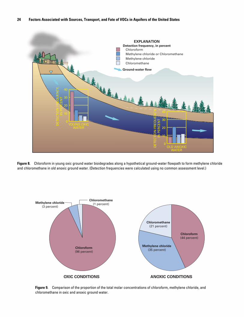
24 Factors Associated with Sources, Transport, and Fate of VOCs in Aquifers of the United States
Detection frequency, in percent
ChloroformMethylene chloride or Chloromethane
Ground-water flow
Methylene chlorideChloromethane
YOUNG OXICWATER
DE
TE
CT
ION
FR
EQ
UE
NC
Y,IN
PE
RC
EN
T
DE
TE
CT
ION
FR
EQ
UE
NC
Y,IN
PE
RC
EN
T
0
10
20
30
40
0
10
20
30
40
OLD ANOXICWATER
EXPLANATION
Figure 8. Chloroform in young oxic ground water bioidegrades along a hypothetical ground-water flowpath to form methylene chloride and chloromethane in old anoxic ground water. (Detection frequencies were calculated using no common assessment level.)
OXIC CONDITIONS ANOXIC CONDITIONS
Chloroform
(96 percent)
Chloroform
(44 percent)
Methylene chloride
(35 percent)
Chloromethane
(21 percent)
Methylene chloride
(3 percent)
Chloromethane
(1 percent)
Figure 9. Comparison of the proportion of the total molar concentrations of chloroform, methylene chloride, and chloromethane in oxic and anoxic ground water.

Analysis of the Sources, Transport, and Fate of VOCs 25
Table 6. Results of a linear regression model of detection frequency of chloroform in 13 selected aquifer studies as the response variable and three explanatory variables partially representing the source, transport, and fate of chloroform.
Dependentvariable
Independent variable Type of variable Unstandardizedcoefficient
Standardizedcoefficient
Detection frequency of chloroform in network
Median dissolved-oxygen concentration in network
Fate 9.93 1.11
Percentage of withdrawal originating from storage in the aquifer
Transport -.90 -.55
Median population density for network Source 5.10 .37
As population density increases (surrogate for the number and strength of anthropogenic sources), the detection frequency of VOCs increases (Squillace and others, 1999); however, in selected aquifer studies, the population density also is corre-lated (Spearman’s rho=0.4, p=0.003) with ground-water recharge in rural and low-density residential areas (fig. 10), where most selected aquifer studies were done. The relation between population density and ground-water recharge has been documented in previous investigations in urban areas (Custodio, 1997; Coldewey and Messer, 1997; Lerner, 2002); however, the three selected aquifer studies done in urban areas by NAWQA had some of the smallest estimates of ground-water recharge (fig. 10). Impervious surfaces are associated with urbanization and result in increased surface runoff; however, in these same areas, irrigation with imported water, leakage from water lines and sewer lines, discharge from septic systems, decreased evapotranspiration, and ground-water recharge from engineered structures (for example, dry wells) could increase ground-water recharge. Correlations between detection frequency of VOCs, population density, and ground-water recharge indicate that areas with larger populations are more vulnerable to ground-water contamination, not only because of the greater number of sources of VOCs but also because greater recharge assists VOC transport to ground water. Even if the relation between population density and recharge is fortuitous—not related to anthropogenic activity but simply a result of where people have chosen to live—the increased recharge would still assist VOC transport through the unsatur-ated zone to ground water.
Use of Mixtures to Determine Significant Associations
Analysis of mixtures of contaminants is a relatively new area of research, but it is particularly pertinent to the selected aquifer studies because many samples contained mixtures of VOCs. Although this mixture analysis is new, it has very impor-tant practical implications in that statistical analysis of the
composition of mixtures can be used to help establish associa-tions with possible sources. Such analysis also can yield addi-tional information on the transport and fate of VOCs. The disad-vantage of mixture analysis is that it can be difficult to understand, perform, and explain. Statistical packages are not designed to do this type of analysis, and even identifying the mixtures is a complicated process.
The detection of mixtures of VOCs is associated with well type. Samples from public-water-supply wells had the largest detection frequency of mixtures, followed by monitoring, irri-gation, and other types of wells; domestic wells had the lowest detection frequency. The reason why samples from public-water supply wells had greater incidence of mixtures than domestic water supplies is not known; however, it could be related to land use and pumping rates. The median amount of urban land use within 500 m of public water supplies was two orders of magnitude greater than that for domestic water supplies. The greater incidence of urban land use near public water supplies is a good indication of more potential sources of VOCs; furthermore, larger pumping rates associated with public water supplies have large capture zones that can integrate more of these sources. Stackelberg and others (2001) also have shown that public supply wells in the Atlantic Coastal Plain aquifer accelerate the vertical gradient and capture ground water with shorter traveltimes than domestic wells. Public supply wells also are more likely than domestic wells to capture ground water that has flowed along extended flowpaths with much longer traveltimes. Short flowpaths with young water could carry recently used VOCs and extended flowpaths with older ground water could carry previously used VOCs and their degradates. The combination of VOCs in short and extended flowpaths makes it more likely to detect multiple VOCs in a single water sample.
Analysis of data indicates no difference in concentrations of VOCs if they occurred alone or in mixtures. Among 10 frequently detected VOCs, 5 (TCA, MTBE, TCE, PCE, and bromodichloromethane) were rarely found by themselves (less than about 10 percent when detected). For these five VOCs, it is impossible to compare concentrations of VOCs occurring

26 Factors Associated with Sources, Transport, and Fate of VOCs in Aquifers of the United States
alone with those in mixtures because of insufficient data. The remaining five VOCs (TMB, chloromethane, methylene chloride, toluene, and chloroform) were found alone about 30 percent of the time when detected. Concentrations of chlo-romethane, methylene chloride, and toluene were not signifi-cantly different if these VOCs were found alone or in mixtures. The concentrations of TMB were significantly smaller in samples with mixtures than samples without mixtures, whereas the concentrations of chloroform were larger in samples with mixtures. Although these differences were statistically signifi-cant, the magnitudes of these differences were very small (medians changed by about 0.01µg/L).
Dissolved oxygen has a dramatic effect on the composition of mixtures. In oxic water, for example, the concentrations of TCE were significantly correlated with five other VOCs; however, in anoxic water, TCE was not correlated with any VOC. Identification of mixtures without regard to dissolved-oxygen concentration (approach taken in this analysis) gives the best indication of mixtures that are most likely to be detected in the ground-water resource, but the approach will result in a bias
toward mixtures common within the dominant redox condition. Data used for this analysis are primarily oxic (two-thirds) with some anoxic samples (one-third).
A mixture that had an actual detection frequency that was similar to the theoretical probability of detection indicates the random co-occurrence of VOCs in the mixture. In contrast, a mixture that had a detection frequency that was much larger than the theoretical probability of detection indicates nonrandom co-occurrence of VOCs in the mixture. The mixtures were ranked according to their DFR, which ranged from 1 to about 3,000 (table 7). Almost all mixtures had a DFR greater than 1, indicating that mixtures normally had detection frequencies greater than what would be expected by chance. Table 8 lists the dectection frequencies of VOCs found in mixtures shown in table 7 and the long-term method detection levels. These estimated detection frequencies are not censored to a common assessment level so direct comparisons of the detection frequencies between individual VOCs may be misleading.
RE
CH
AR
GE
, IN
MIL
LIM
ET
ER
S P
ER
YE
AR
NATURAL LOGARITHM OF POPULATION DENSITY,PEOPLE PER SQUARE KILOMETER
500
400
300
200
100
0-1 0 1 2 3 4 5 6 7 8
Rural Low-densityResidential
Urban
Figure 10. Significant correlation between population density and estimated recharge for each selected aquifer study sampled by the National Water-Quality Assessment Program.
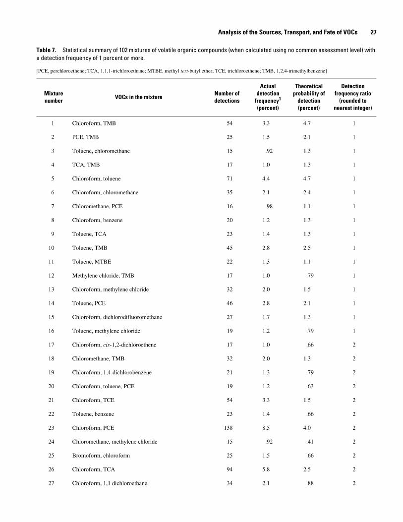
Analysis of the Sources, Transport, and Fate of VOCs 27
Table 7. Statistical summary of 102 mixtures of volatile organic compounds (when calculated using no common assessment level) with a detection frequency of 1 percent or more.
[PCE, perchloroethene; TCA, 1,1,1-trichloroethane; MTBE, methyl tert-butyl ether; TCE, trichloroethene; TMB, 1,2,4-trimethylbenzene]
Mixturenumber
VOCs in the mixtureNumber of detections
Actual detection
frequency1
(percent)
Theoretical probability of
detection(percent)
Detection frequency ratio
(rounded to nearest integer)
1 Chloroform, TMB 54 3.3 4.7 1
2 PCE, TMB 25 1.5 2.1 1
3 Toluene, chloromethane 15 .92 1.3 1
4 TCA, TMB 17 1.0 1.3 1
5 Chloroform, toluene 71 4.4 4.7 1
6 Chloroform, chloromethane 35 2.1 2.4 1
7 Chloromethane, PCE 16 .98 1.1 1
8 Chloroform, benzene 20 1.2 1.3 1
9 Toluene, TCA 23 1.4 1.3 1
10 Toluene, TMB 45 2.8 2.5 1
11 Toluene, MTBE 22 1.3 1.1 1
12 Methylene chloride, TMB 17 1.0 .79 1
13 Chloroform, methylene chloride 32 2.0 1.5 1
14 Toluene, PCE 46 2.8 2.1 1
15 Chloroform, dichlorodifluoromethane 27 1.7 1.3 1
16 Toluene, methylene chloride 19 1.2 .79 1
17 Chloroform, cis-1,2-dichloroethene 17 1.0 .66 2
18 Chloromethane, TMB 32 2.0 1.3 2
19 Chloroform, 1,4-dichlorobenzene 21 1.3 .79 2
20 Chloroform, toluene, PCE 19 1.2 .63 2
21 Chloroform, TCE 54 3.3 1.5 2
22 Toluene, benzene 23 1.4 .66 2
23 Chloroform, PCE 138 8.5 4.0 2
24 Chloromethane, methylene chloride 15 .92 .41 2
25 Bromoform, chloroform 25 1.5 .66 2
26 Chloroform, TCA 94 5.8 2.5 2
27 Chloroform, 1,1 dichloroethane 34 2.1 .88 2

28 Factors Associated with Sources, Transport, and Fate of VOCs in Aquifers of the United States
28 Chloroform, MTBE 84 5.2 2.2 2
29 Styrene, TMB 15 .92 .37 2
30 Chloroform, trichlorofluoromethane 25 1.5 .59 3
31 Chloroform, toluene, TCA 16 .98 .39 3
32 Benzene, TMB 28 1.7 .67 3
33 Chloroform, 1,1-dichloroethene 31 1.9 .68 3
34 TMB, m,p-xylene 20 1.2 .39 3
35 Toluene m,p-xylene 20 1.2 .39 3
36 Chloroform, trichlorotrifluoromethane 15 .92 .31 3
37 Toluene, styrene 19 1.2 .37 3
38 PCE, 1,4-dichlorobenzene 18 1.1 .35 3
39 PCE, MTBE 49 3.0 .98 3
40 Chlorodibromomethane, chloroform 32 2.0 .59 3
41 PCE, TCA 61 3.7 1.1 3
42 PCE, cis-1,2-dichloroethene 18 1.1 .30 4
43 PCE, trichlorofluoromethane 19 1.2 .26 4
44 TCE, MTBE 24 1.5 .36 4
45 TCA, MTBE 38 2.3 .61 4
46 TCA, TCE 31 1.9 .41 5
47 PCE, 1,1-dichloroethane 29 1.8 .39 5
48 PCE, TCE 56 3.4 .66 5
49 1,1-Dichloroethane, TCA 21 1.3 .25 5
50 Trichlorofluoromethane, TCA 15 .92 .16 6
51 PCE, 1,1-dichloroethene 31 1.9 .30 6
52 1,1 Dichloroethane, MTBE 22 1.3 .21 6
53 1,1-Dichloroethene, TCA 23 1.4 .19 7
54 1,1-Dichloroethane, TCE 22 1.3 .14 9
Table 7. Statistical summary of 102 mixtures of volatile organic compounds (when calculated using no common assessment level) with a detection frequency of 1 percent or more.—Continued
[PCE, perchloroethene; TCA, 1,1,1-trichloroethane; MTBE, methyl tert-butyl ether; TCE, trichloroethene; TMB, 1,2,4-trimethylbenzene]
Mixturenumber
VOCs in the mixture Number of detections
Actual detection
frequency1
(percent)
Theoretical probability of
detection(percent)
Detection frequency ratio
(rounded to nearest integer)

Analysis of the Sources, Transport, and Fate of VOCs 29
55 Chloroform, PCE, MTBE 45 2.8 0.29 9
56 Trichlorofluoromethane, TCE 16 .98 .096 10
57 Chloroform, PCE, TCA 54 3.3 .33 10
58 Chloroform, TCE, MTBE 20 1.2 .11 11
59 Chloroform, TCA, MTBE 36 2.2 .18 12
60 Chloroform, TCA, TCE 27 1.7 .12 13
61 Chloroform, PCE, trichlorofluoromethane 18 1.1 .079 14
62 1,1-Dichloroethene, TCE 25 1.5 .11 14
63 Chloroform, PCE, 1,1-dichloroethane 27 1.7 .12 14
64 TCE, cis-1,2-dichloroethene 26 1.6 .11 15
65 Chloroform, PCE, TCE 48 2.9 .20 15
66 1,1-Dichloroethane, cis-1,2-dichloroethene 16 .98 .065 15
67 Chloroform, 1,1-dichloroethane, MTBE 16 .98 .064 15
68 Chloroform, 1,1-dichloroethane, TCA 19 1.2 .073 16
69 1,1-Dichloroethane, 1,1-dichloroethene 20 1.2 .067 18
70 PCE, TCA, MTBE 26 1.6 .081 20
71 Chloroform, PCE, 1,1-dichloroethene 30 1.8 .091 20
72 Bromoform, chlorodibromomethane 17 1.0 .04 24
73 Chloroform, 1,1-dichloroethene, TCA 22 1.3 .057 24
74 PCE, TCE, MTBE 20 1.2 .048 26
75 Chloroform, TCE, cis-1,2-dichloroethene 16 .98 .032 30
76 Chloroform, 1,1-dichloroethane, TCE 21 1.3 .043 30
77 PCE, 1,1-dichloroethane, TCA 16 .98 .033 30
78 TCA, TCE, MTBE 15 .92 .030 31
79 PCE, TCA, TCE 29 1.8 .055 32
80 Chloroform, trichlorofluoromethane, TCE 16 .98 .029 34
81 Chloroform, 1,1-dichloroethene, TCE 23 1.4 .033 42
Table 7. Statistical summary of 102 mixtures of volatile organic compounds (when calculated using no common assessment level) with a detection frequency of 1 percent or more.—Continued
[PCE, perchloroethene; TCA, 1,1,1-trichloroethane; MTBE, methyl tert-butyl ether; TCE, trichloroethene; TMB, 1,2,4-trimethylbenzene]
Mixturenumber
VOCs in the mixture Number of detections
Actual detection
frequency1
(percent)
Theoretical probability of
detection(percent)
Detection frequency ratio
(rounded to nearest integer)
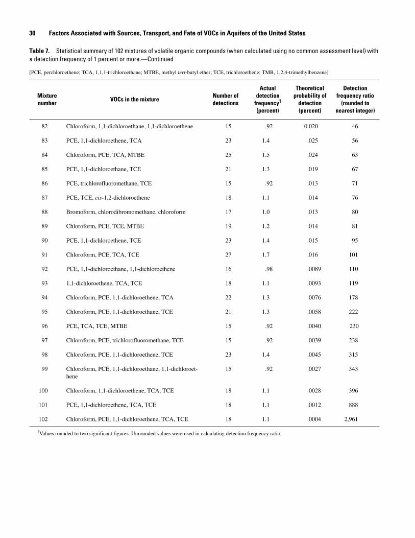
30 Factors Associated with Sources, Transport, and Fate of VOCs in Aquifers of the United States
82 Chloroform, 1,1-dichloroethane, 1,1-dichloroethene 15 .92 0.020 46
83 PCE, 1,1-dichloroethene, TCA 23 1.4 .025 56
84 Chloroform, PCE, TCA, MTBE 25 1.5 .024 63
85 PCE, 1,1-dichloroethane, TCE 21 1.3 .019 67
86 PCE, trichlorofluoromethane, TCE 15 .92 .013 71
87 PCE, TCE, cis-1,2-dichloroethene 18 1.1 .014 76
88 Bromoform, chlorodibromomethane, chloroform 17 1.0 .013 80
89 Chloroform, PCE, TCE, MTBE 19 1.2 .014 81
90 PCE, 1,1-dichloroethene, TCE 23 1.4 .015 95
91 Chloroform, PCE, TCA, TCE 27 1.7 .016 101
92 PCE, 1,1-dichloroethane, 1,1-dichloroethene 16 .98 .0089 110
93 1,1-dichloroethene, TCA, TCE 18 1.1 .0093 119
94 Chloroform, PCE, 1,1-dichloroethene, TCA 22 1.3 .0076 178
95 Chloroform, PCE, 1,1-dichloroethane, TCE 21 1.3 .0058 222
96 PCE, TCA, TCE, MTBE 15 .92 .0040 230
97 Chloroform, PCE, trichlorofluoromethane, TCE 15 .92 .0039 238
98 Chloroform, PCE, 1,1-dichloroethene, TCE 23 1.4 .0045 315
99 Chloroform, PCE, 1,1-dichloroethane, 1,1-dichloroet-hene
15 .92 .0027 343
100 Chloroform, 1,1-dichloroethene, TCA, TCE 18 1.1 .0028 396
101 PCE, 1,1-dichloroethene, TCA, TCE 18 1.1 .0012 888
102 Chloroform, PCE, 1,1-dichloroethene, TCA, TCE 18 1.1 .0004 2,961
1Values rounded to two significant figures. Unrounded values were used in calculating detection frequency ratio.
Table 7. Statistical summary of 102 mixtures of volatile organic compounds (when calculated using no common assessment level) with a detection frequency of 1 percent or more.—Continued
[PCE, perchloroethene; TCA, 1,1,1-trichloroethane; MTBE, methyl tert-butyl ether; TCE, trichloroethene; TMB, 1,2,4-trimethylbenzene]
Mixturenumber
VOCs in the mixture Number of detections
Actual detection
frequency1
(percent)
Theoretical probability of
detection(percent)
Detection frequency ratio
(rounded to nearest integer)
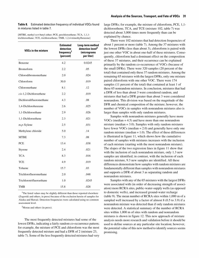
Analysis of the Sources, Transport, and Fate of VOCs 31
Table 8. Estimated detection frequency of individual VOCs found in mixtures listed in table 7.
[MTBE, methyl tert-butyl either; PCE, perchloroethene; TCA, 1,1,1-trichloroethane; TCE, trichloroethene; TMB, 1,2,4-trimethylbenzene]
VOCs in the mixture
Estimateddetection
frequency1
(percent)
Long-term method detection level2
(microgramsper liter)
Benzene 4.2 0.0245
Bromoform 2.2 .05
Chlorodibromomethane 2.0 .024
Chloroform 30.0 .019
Chloromethane 8.1 .12
cis-1,2-Dichloroethene 2.2 .019
Dichlorodifluoromethane 4.3 .08
1,4-Dichlorobenzene 2.6 .025
1,1-Dichloroethane 2.9 .026
1,1-Dichloroethene 2.3 .021
m,p-Xylene 2.5 .031
Methylene chloride 5.0 .14
MTBE 7.3 .08
PCE 13.4 .038
Styrene 2.4 .021
TCA 8.3 .016
TCE 4.9 .019
Toluene 15.7 .03
Trichlorofluoromethane 2.0 .048
Trichlorotrifluoroethane 1.0 .0245
TMB 15.8 .028
1The listed values may be slightly different than those reported elsewhere (Zogorski and others, in press) because of the exclusion herein of samples for Alaska and Hawaii. Detection frequencies were calculated using no common assessment level.
2Moran and others (in press).
The most frequently detected mixtures had some of the lowest DFRs, indicating a fairly random co-occurrence pattern; for example, the mixture of PCE and chloroform was the most frequently detected mixture and had a DFR of 2 (mixture 23, table 7). Some of the less frequently detected mixtures had very
large DFRs; for example, the mixture of chloroform, PCE, 1,1-dichloroethene, TCA, and TCE (mixture 102, table 7) was detected about 3,000 times more frequently than can be explained by chance.
There were 102 mixtures that had detection frequencies of about 1 percent or more (table 7). Among the 37 mixtures with the lowest DFRs (less than about 3), chloroform is paired with just one other VOC in about one-half of these mixtures. Conse-quently, chloroform had a dominant effect on the composition of these 37 mixtures, and their occurrence can be explained primarily by the random co-occurrence of VOCs (because of the small DFRs). There were 320 samples (20 percent of the total) that contained only these 37 random mixtures. Among the remaining 65 mixtures with the largest DFRs, only one mixture paired chloroform with one other VOC. There were 174 samples (11 percent of the total) that contained at least 1 of these 65 nonrandom mixtures. In conclusion, mixtures that had a DFR of less than about 3 were considered random, and mixtures that had a DFR greater than about 3 were considered nonrandom. This division was based on the magnitude of the DFR and chemical composition of the mixture; however, the number of VOCs in samples with nonrandom mixtures also is larger than samples with only random mixtures.
Samples with nonrandom mixtures generally have more VOCs (median = 4.5) and have more than one nonrandom mixture (median = 3.0). Samples with only random mixtures have fewer VOCs (median = 2.0) and generally have only one random mixture (median = 1.0). The effect of these differences is illustrated in figure 11, which shows how the cumulative number of samples with mixtures increases with the inclusion of each mixture (starting with the most nonrandom mixture). The slopes of the two regression lines in figure 11 show that with the inclusion of each nonrandom mixture, only 1.3 new samples are identified; in contrast, with the inclusion of each random mixture, 9.3 new samples are identified. All these differences demonstrate how samples with random mixtures are fundamentally different than samples with nonrandom mixtures and supports a DFR of about 3 as separating random and nonrandom mixtures.
Samples with any of the 65 mixtures with the largest DFRs were associated with (in order of decreasing strength of associ-ation) more RCRA sites, public-water-supply wells (as opposed to domestic wells), and increased ground-water recharge (table 9). The mean number of RCRA sites within 1,000 m of a sampled well increased by a factor of almost 8 (0.5 to 3.9) if a nonrandom mixture was detected than if only random mixtures were detected. A statistical summary of the number of RCRA sites within 1,000 m of sites with random and nonrandom mixtures is shown in figure 12. This new approach of mixture analysis needs more research and validation before it should be used to define sources at any particular site location; however, the potential value of this new method to identify sources seems promising.

32 Factors Associated with Sources, Transport, and Fate of VOCs in Aquifers of the United States
CUM
ULA
TIV
E N
UM
BE
R O
F S
AM
PLE
S W
ITH
MIX
TU
RE
S
MIXTURE NUMBER (see table 6)
600
500
400
300
200
100
0110 8090100 70 60 50 40 30 20 10 0
Random mixtures
Nonrandom mixtures
Figure 11. Relation between the cumulative number of samples and the type of mixture.
Table 9. Logistic regression analysis for samples with random/nonrandom mixtures.
Dependentvariable Independent variable
Type ofvariable
Unstandardizedcoefficient
Standardizedcoefficient
Random/nonrandom mixtures (random mixtures=0, nonrandom mixtures=1)
Number of Resource Conservation and Recovery Act (RCRA) sites within 1 kilometer
Source 0.130 0.27
Domestic/public water supply well (domestic water supply=0, public water supply=1)
Indeterminate 1.500 .25
Estimated ground-water recharge within 500-meter circular buffer around sampled well
Transport .003 .17
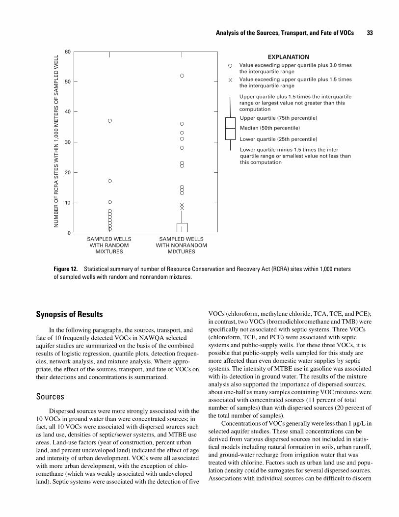
Analysis of the Sources, Transport, and Fate of VOCs 33
Value exceeding upper quartile plus 3.0 timesthe interquartile range
Value exceeding upper quartile plus 1.5 timesthe interquartile range
Median (50th percentile)
Lower quartile (25th percentile)
Upper quartile (75th percentile)
Lower quartile minus 1.5 times the inter-quartile range or smallest value not less thanthis computation
Upper quartile plus 1.5 times the interquartilerange or largest value not greater than thiscomputation
EXPLANATIONN
UM
BE
R O
F R
CR
A S
ITE
S W
ITH
IN 1
,000
ME
TE
RS
OF
SA
MP
LED
WE
LL60
50
40
30
20
10
0SAMPLED WELLSWITH RANDOM
MIXTURES
SAMPLED WELLSWITH NONRANDOM
MIXTURES
Figure 12. Statistical summary of number of Resource Conservation and Recovery Act (RCRA) sites within 1,000 meters of sampled wells with random and nonrandom mixtures.
Synopsis of Results
In the following paragraphs, the sources, transport, and fate of 10 frequently detected VOCs in NAWQA selected aquifer studies are summarized on the basis of the combined results of logistic regression, quantile plots, detection frequen-cies, network analysis, and mixture analysis. Where appro-priate, the effect of the sources, transport, and fate of VOCs on their detections and concentrations is summarized.
Sources
Dispersed sources were more strongly associated with the 10 VOCs in ground water than were concentrated sources; in fact, all 10 VOCs were associated with dispersed sources such as land use, densities of septic/sewer systems, and MTBE use areas. Land-use factors (year of construction, percent urban land, and percent undeveloped land) indicated the effect of age and intensity of urban development. VOCs were all associated with more urban development, with the exception of chlo-romethane (which was weakly associated with undeveloped land). Septic systems were associated with the detection of five
VOCs (chloroform, methylene chloride, TCA, TCE, and PCE); in contrast, two VOCs (bromodichloromethane and TMB) were specifically not associated with septic systems. Three VOCs (chloroform, TCE, and PCE) were associated with septic systems and public-supply wells. For these three VOCs, it is possible that public-supply wells sampled for this study are more affected than even domestic water supplies by septic systems. The intensity of MTBE use in gasoline was associated with its detection in ground water. The results of the mixture analysis also supported the importance of dispersed sources; about one-half as many samples containing VOC mixtures were associated with concentrated sources (11 percent of total number of samples) than with dispersed sources (20 percent of the total number of samples).
Concentrations of VOCs generally were less than 1 µg/L in selected aquifer studies. These small concentrations can be derived from various dispersed sources not included in statis-tical models including natural formation in soils, urban runoff, and ground-water recharge from irrigation water that was treated with chlorine. Factors such as urban land use and popu-lation density could be surrogates for several dispersed sources. Associations with individual sources can be difficult to discern

34 Factors Associated with Sources, Transport, and Fate of VOCs in Aquifers of the United States
with statistical methods because (1) the results depend on the accuracy of the ancillary information, and (2) VOCs can origi-nate from a variety of dispersed and concentrated sources, have multiple sources (even at one location), and result from the degradation of other VOCs.
Small concentrations of certain VOCs detected in selected aquifer studies also were associated with concentrated sources, for example, gasoline LUST sites and RCRA sites. Processes such as dispersion and degradation can reduce concentrations from these sources so that detected concentrations are similar to those from dispersed sources. Seven VOCs (all except bromod-ichloromethane, chloromethane, and methylene chloride) were associated with a concentrated source; however, these sources were not as strong as dispersed sources. Concentrated sources can supply more than one VOC; however, VOC concentrations in samples with mixtures compared with samples without mixtures showed that the difference in concentration was not statistically significant or was not environmentally important. These overall results show that the detection of small concen-trations of VOCs in selected aquifer studies cannot be used exclusively to classify the type of source.
Transport
A VOC detected in ground water would, in general, require first a release from a source and then subsequent trans-port to ground water. Factors that potentially affect the transport of VOCs to ground water are dependent on where the release occurred. If the release is at land surface (for example, a spill), climate and near-surface soil characteristics could affect trans-port to ground water. If the release is below land surface (for example, LUST sites or septic systems/sewer lines), climate would be less important; furthermore, soil characteristics at land surface also might not be relevant unless they are represen-tative of material deeper in the unsaturated zone. Ground-water recharge could, however, be an important transport factor within the unsaturated zone. Once in the aquifer, VOCs are transported by advective ground-water flow and dispersion.
Cool temperature was an important transport factor for the detection of four VOCs (TCA, MTBE, TMB, and toluene). In cool climates, evaporation of MTBE, TMB, and toluene from a gasoline spill would be reduced, increasing the potential of these VOCs to infiltrate to ground water with recharge water. Multiple VOCs in a single source could, however, become separated by in-situ processes such as sorption. Furthermore, some VOCs could evaporate from a gasoline spill while others could move to the top of shallow ground water with recharge water. Concentrations of MTBE in urban air appear sufficiently large in some areas to account for some concentrations of MTBE detected in shallow ground water (Zogorski and others, in press), assuming that equilibrium is achieved between urban air, soil gas, and the top of the water table. Ambient air concen-trations in rural areas likely are not large enough to account for concentrations of MTBE detected in selected aquifer studies.
Several soil characteristics were important for the detec-tion of six VOCs (chloroform, TCE, toluene, chloromethane, methylene chloride, and TCA). A soil is classified as hydric if it is sufficiently wet in the upper part to develop anoxic condi-tions during the growing season; consequently, this soil charac-teristic could be more related to the fate of VOCs than to trans-port. Nevertheless, chloroform and TCE were associated with non-hydric soils (oxic conditions), and toluene was associated with hydric soils (anoxic conditions). Percent sand and silt is related to soil permeability. Two VOCs (chloromethane and methylene chloride) were associated with less permeable soils. If these VOCs are degradation products of chloroform, then slow movement of water through the unsaturated zone may promote the degradation of chloroform and formation of its two degradation products. Sorption to organic carbon would slow the movement of VOCs through the unsaturated zone and within an aquifer; however, TCA was the only VOC associated with low organic carbon content in soils. Organic carbon in soils or aquifer material could also result in the separation of a mixture of VOCs (depending on their solubility in water) as they are transported through soil or an aquifer.
High rates of ground-water recharge were associated with the detection of chloroform, TCE, and MTBE; in contrast, low recharge rates were associated with the detection of bromod-ichloromethane and TMB. VOCs are more frequently detected in more populated areas for two reasons: (1) the number of sources increase, and (2) recharge increases (fig. 10), hastening transport of VOCs through the unsaturated zone to ground water and reducing the opportunity for degradation. This means that one would expect high ground-water recharge rates to be associated with more frequent detections of VOCs in ground water. VOCs associated with low recharge rates are more diffi-cult to explain, but they could be related to the source. If a source (for example, a leaky sewer line) releases a small volume and small concentrations of particular VOCs (for example, bromodichloromethane and TMB), then recharge water could dilute concentrations to below the reporting level. Concentrated sources probably are less affected by recharge than dispersed sources are.
Confining layers can prevent ground-water recharge (and VOCs) from reaching an aquifer; however, confined aquifers were not associated with fewer VOC detections compared with unconfined aquifers. This finding could mean that, in general, the presence of a confining unit does not adequately protect ground water from anthropogenic contamination.
The transport of VOCs within an aquifer was found to be affected by well depth and the percentage of ground-water with-drawal in the aquifer coming from a decrease in storage (water removed from the aquifer that probably is a one-time with-drawal). Shallow well depth (table 5) was an important factor in the detection of four VOCs (methylene chloride, TCA, PCE, and MTBE). Traveltimes to deeper wells generally is longer, allowing more time for degradation along the flowpath. In some situations, water is sufficiently old that no anthropogenic sources of VOCs existed when ground water was recharged. Source of water to a well, direction of ground-water flow, trav-
Implications for Ground-Water Management and Assessments 35
eltimes, and recharge rates can be helpful in explaining the detection of VOCs at a particular location; however, regional ground-water-flow models also can be used to help explain the detection of VOCs in selected aquifer studies. A comparison of regional ground-water-flow models can show major differences in how aquifers respond to withdrawal and the source of water to the aquifers. These differences can be used to explain differ-ences in detection frequencies of some VOCs in selected aquifer studies.
Fate
Dissolved-oxygen concentration was the most frequently occurring explanatory factor in logistic regression models for the 10 VOCs. Seven VOCs were associated with oxic condi-tions (bromodichloromethane, chloroform, TCA, TCE, PCE, MTBE, and toluene), and only one VOC (chloromethane) was associated with anoxic conditions. These results are particularly important because this multivariate analysis controls for differ-ences such as climate and hydrogeologic factors that also can affect the detection of VOCs in ground water. A comparison of detection frequencies of the 10 VOCs in oxic and anoxic condi-tions (fig. 6) generally supports the results of the logistic regres-sion analysis; however, methylene chloride had significantly larger detection frequency in anoxic conditions than in oxic conditions, but logistic regression analysis did not identify oxic/anoxic conditions as being a significant explanatory factor. For the network analysis, the median dissolved-oxygen concentra-tion in a selected aquifer study was a significant explanatory factor for the detection frequency of chloroform.
Dissolved-oxygen concentrations in ground water not only affected the detection but also the concentrations of VOCs. Quantile/quantile plots showed that the amount of dissolved oxygen affected the concentrations of eight VOCs and are generally consistent with results from logistic regression and detection-frequency analysis. Methylene chloride, however, had significantly larger concentrations and detection frequen-cies in anoxic water, but logistic regression analysis did not identify this VOC as being associated with anoxic water. Toluene also did not have significantly different concentrations or detection frequencies in either oxygen condition, but logistic regression analysis showed an association with oxic conditions. These results indicate that univariate analyses such as quantile/quantile plots and analysis of detection frequencies can produce conflicting results when compared with multivariate analysis. Multivariate analyses, however, probably are better because they control for a variety of factors that can affect the detection of VOCs. Quantile plots showed that the effect of anthropo-genic activity on ground-water quality can depend on oxygen concentrations. Chloroform is more stable in oxic than anoxic conditions; therefore, the effect of urban land use and the use of septic systems (both surrogates for chloroform sources) on the concentrations of chloroform was greater for oxic conditions than anoxic conditions.
Implications for Ground-Water Management and Assessments
Objectives of large-scale ground-water resource assess-ments often involve evaluating the occurrence, distribution, and status of contaminants in ground water; however, the value of these assessments could be enhanced if determining the sources, transport, and fate of contaminants also was part of the project objectives and analyses. For example, if associations can be established between VOCs in ground water and explan-atory factors in a particular study area, then one could extrapo-late the results into similar areas where water-quality informa-tion has not been collected. One might also be able to estimate the risk of ground-water contamination in similar hydrogeo-logic areas if certain types of development are allowed. Large aquifers can have many sources of anthropogenic contamina-tion; consequently, the most important contaminant source for a particular aquifer can be difficult to identify. If, however, accurate ancillary information is combined with accurate water-quality data from resource assessments, hypotheses derived from small-scale studies also can be tested for their relevance at a larger scale; conversely, hypotheses derived from large-scale resource assessment can be used to prioritize and design small-scale research projects that address potentially important issues for large aquifers.
Accurate ancillary data related to sources, transport, and fate of VOCs is essential to establishing reliable associations with occurrence and concentrations of VOCs in ground-water resource assessments. Collecting ancillary information in a circular buffer around the sampled well is adequate for some analysis. The assumption behind this approach is that land use within the buffer is representative of land use in the true capture zone of the sampled well, even if it lies beyond the buffer. Ground-water-flow models can provide better estimates of the locations of the capture zones of public-supply wells; however, this approach probably is not feasible for domestic water supplies because of the small amount of withdrawal.
Sources
The best possible information on the location, nature, timing, and amount of any release of VOCs is needed along with general information on land-use activities. Land-use activ-ities within circular buffers around wells can be associated with ground-water quality, but incremental improvements to this approach are possible if more is known about the direction of ground-water flow in the vicinity of the well. For completeness of ancillary data, both concentrated and dispersed sources of contamination should be delineated because both can result in small concentrations in ambient ground water. The known release of VOCs from a concentrated source at a particular loca-tion can be used to establish associations with VOCs in ground water. Small concentrations of VOCs that originate from concentrated sources could be a concern because they can

36 Factors Associated with Sources, Transport, and Fate of VOCs in Aquifers of the United States
increase with time. Concentrations also would be expected to increase closer to the source.
General land-use activities—for example, the amount of urban land use—also can be helpful in estimating input from dispersed sources; however, these types of associations are not as helpful as delineating a particular dispersed source, such as a subdivision served by septic systems. Potential sources that are found not to be associated with any contamination also are important because they help identify anthropogenic activity that does not pose a threat to ground-water quality. VOCs in ground water that are associated with septic systems may not present a substantial concern to human health; however, the presence of these VOCs could indicate the presence of other chemicals or bacteria associated with wastewater. Public-water-supply wells may be more affected by septic systems than domestic water supplies for some VOCs, probably because of the larger pumping rates and larger capture zones for public-supply wells compared with domestic wells. More research is needed to define the effect of septic systems on ground-water quality, in particular how the use of household products like bleach could contribute to the detection of chloroform in ground water or how improper disposable of solvents and other VOCs in septic systems also could contribute to the detection of other VOCs like toluene, PCE, and TCE.
Transport
Well depth/screen depth, ground-water recharge/precipita-tion, air temperature, and soil characteristics were significant factors in helping explain the transport of VOCs to ground water. The availability of simple data such as well depth and depth to the top of the screened interval could be used in well-selection and sampling criteria because of their value in explaining the detection of VOCs in ground water. Estimates of ground-water recharge, precipitation, and air temperature are available for most of the Nation, although the quality of these estimates varies. Chemical and hydrologic characteristics of soils and aquifers can be more difficult to obtain, but these factors are important to adequately explain the transport of VOCs.
The transport of VOCs can be best understood by defining the direction of ground-water flow and developing ground-water-flow models at various scales (small to regional). If the direction of ground-water flow is known, then land-use activi-ties and hydrogeologic factors downgradient from the sampled well generally can be disregarded unless the sampling point is a public-supply well. For public-supply wells, a more sophisti-cated approach (but also more costly) would be to use small-scale flow models to estimate the location of the capture zone; defining capture zones for domestic-supply wells would be very difficult because of the small pumping rates associated with these wells. Ground-water-flow models may still not precisely define the capture zones to public-supply wells, but a simulated capture zone as an area for determining land-use activity prob-ably is better than a circular buffer. Sources in the defined
capture zone could then be related to water quality depending on traveltimes of ground water to the pumping well.
Large-scale ground-water-flow-models can be used to understand the source of water to an aquifer and the way that pumping affects the overall ground-water-flow system. These models can show important differences between regional aqui-fers. Aquifers can differ in lithology, which is sometimes used as a surrogate for hydrogeologic characteristics; however, lithology has limitations because it is not quantitative, is subject to individual interpretation, and it represents only part of the flow system. Many hydrogeologic factors within regional aqui-fers also can vary tremendously; in fact, this variability can be larger than variability between regional aquifers making it diffi-cult to distinguish aquifers on the basis of one factor. Flow models can include the effect of many hydrogeologic factors, are quantitative, can be developed at different scales, and can improve with time as additional data are collected for better model calibration. These models can, for example, help deter-mine whether most of the ground water is coming from induced infiltration from a different aquifer, storage, or intercepted stream discharge. Differences in the quality of water derived from these different sources could be substantial. A comparison of water budgets between various regional aquifers may help explain differences in the water quality and may be helpful in managing the ground-water resource.
VOCs typically are transported through the unsaturated zone to ground water with recharge water; nevertheless, for some VOCs, increased recharge could dilute concentrations in ground water. For example, if a particular VOC comes from small amount of leakage from sewer lines or occurs naturally within the unsaturated zone, then larger amounts of natural recharge could dilute concentrations of this VOC in ground water.
Fate
The fate of VOCs in ground water was explained largely by dissolved-oxygen concentration in ground water. Individual VOCs generally are not equally stable in oxic and anoxic condi-tions; therefore, conditions that favor slower degradation result in increased concentrations and detection frequencies. Dissolved-oxygen data (or, even better, delineation of redox condition) can be used in the analysis of data from monitoring networks to (1) help explain variability in concentrations and detections of VOCs, (2) identify VOCs that are expected to be stable in the sampled ground water and therefore can be used as an early warning for more serious contamination, (3) define more accurately the effects of certain anthropogenic activities on ground-water quality by controlling for differences in dissolved-oxygen concentration, and (4) help determine whether certain VOCs are potential degradation products of other VOCs. If dissolved oxygen/redox changes along a flow-path, it may be more difficult to use in explanatory analysis of monitoring network data.
Summary 37
Well Type
Certain VOCs are more strongly associated with domestic wells, whereas other VOCs are more strongly associated with public-supply wells even after controlling for differences in factors such as land use, dissolved oxygen, and well depth. The effect of well type on the detection frequencies of some VOCs, for example chloroform (fig. 5), may only be apparent in oxygen conditions that favor the preservation of the VOCs. Differences in traveltimes and sources of VOCs near the wells could explain the association of a VOC with a particular type of well. An association of a VOC with a particular well type means higher detection frequencies in one well type compared to another; it does not mean an absence of detections in a partic-ular type of well. These associations could be used to help identify which VOCs to include in the laboratory analysis. The variance in monitoring networks can be reduced by limiting the types of wells selected for sampling, or at least by controlling for well type in the analysis of the data.
Mixtures
VOCs commonly were found in mixtures. Analysis of mixtures of VOCs has the potential to provide greater insight into the interpretation of monitoring data. For example, small concentrations of individual VOCs in a mixture of VOCs in a ground-water sample may not exceed any individual drinking-water standard; however, if the mixture is nonrandom, prox-imity to a concentrated source of VOCs could be indicated, and additional monitoring may be warranted. This preliminary method of mixture analysis used for this report needs to be veri-fied at different reporting levels and with other environmental data.
The health consequence of mixtures of contaminants in potable water is not yet understood. Health risk associated with contaminants in drinking water typically is based on animal studies done at large concentrations for one contaminant over a short period of time. The relevance of these animal studies to human health often is debated because the effect of contami-nants on animals may not be identical to that on humans, and extrapolating effects of exposure to large concentrations to smaller environmental concentrations in drinking water is uncertain. Tracking human health associated with the use of water with a known quality could take years to develop, but the human-health benefits could be substantial. These data could even be compared with risk estimates that are currently being used to establish drinking-water standards.
Summary
Factors associated with sources, transport, and fate of 10 frequently detected volatile organic compounds (VOCs) in selected aquifer systems of the United States were evaluated using various statistical methods. VOC data from 1,631 wells
sampled between 1996 and 2002 as part of the National Water-Quality Assessment (NAWQA) Program of the U.S. Geological Survey were used in the analyses. These samples were a subset of samples included in the Program’s national VOC assessment. Sampled wells were randomly selected from aquifers used to supply drinking water in the regional study areas. Samples were analyzed for 53 VOCs from primarily domestic water supplies (1,184), followed by public-supply wells (216); the remaining wells (231) were from monitoring and other well types. The median well depth was 50 m. Age-date information, available from 44 percent of the sampled wells, shows that about 60 percent of the sampled water was recharged after 1953. Ten VOCs that had a detection frequency of about 5 percent or greater when calculated using no assessment level were selected for more detailed statistical analysis. These compounds are bromodichloromethane, chloroform, chloromethane, meth-ylene chloride, 1,1,1-trichloroethane (TCA), trichloroethene (TCE), perchloroethene (PCE), methyl-tert-butyl ether (MTBE), 1,2,4-trimethylbenzene (TMB), and toluene. Concen-trations of VOCs generally were less than 1 microgram per liter.
A VOC detected in ground water would, in general, require first a release from a source and then subsequent trans-port to ground water. Source factors, in order of decreasing importance, were general land-use activity (dispersed source), septic/sewer density (dispersed source), and sites where large concentrations of VOCs are potentially released (concentrated sources), such as leaking underground storage tanks (LUSTs). All 10 of the VOCs included in this analysis were associated with dispersed sources such as land use, densities of septic/sewer systems, and methyl-tert-butyl-ether-use areas. Three VOCs (chloroform, TCE, and PCE) were associated with septic systems and public-supply wells. For these three VOCs, it is possible that public-supply wells sampled for this study are more affected by septic systems than even domestic water supplies. Factors such as urban land use and densities of septic/sewer systems also could be surrogates for several dispersed sources. Small concentrations of certain VOCs detected in selected aquifer studies also were associated with concentrated sources, for example, gasoline leaking underground storage tank sites and Resource Conservation and Recovery Act sites. Processes such as advection, dispersion, and degradation can reduce concentrations from these sources so that detected concentrations are similar to those from dispersed sources. Seven VOCs (all except bromodichloromethane, chlo-romethane, and methylene chloride) were associated with a concentrated source; however, these sources were not as strong as dispersed sources. Mixture analysis showed that 11 percent of all samples had VOC mixtures that were associated with concentrated sources; 20 percent were associated with dispersed sources. These overall results show that the detection of small concentrations of VOCs in selected aquifer studies cannot be used exclusively to classify the type of source.
Important transport factors included well depth, screen depth, precipitation/recharge, air temperature, soil characteris-tics, and amount of water removed from storage during with-
38 Factors Associated with Sources, Transport, and Fate of VOCs in Aquifers of the United States
drawal from the aquifer. Factors that potentially affect the trans-port of VOCs to ground water are dependent on where the release occurred. If the release is at land surface (for example, a spill), climate and near-surface soil characteristics could affect transport to ground water. If the release is below land surface (for example, LUST sites or septic systems/sewer lines), climate would be less important; furthermore, soil characteris-tics at land surface also might not be relevant unless they are representative of material deeper in the unsaturated zone. Ground-water recharge could, however, be an important trans-port factor within the unsaturated zone. VOCs are more frequently detected in more populated areas for two reasons: (1) the number of sources increase, and (2) recharge increases, hastening transport of VOCs through the unsaturated zone to ground water and reducing the opportunity for degradation. Confining layers can prevent ground-water recharge (and VOCs) from reaching an aquifer; however, confined aquifers were not associated with fewer VOC detections compared with unconfined aquifers. It appears that confining layers do not provide a substantial protection against the infiltration of VOCs. Cool temperature was an important transport factor for the detection of four VOCs (TCA, MTBE, TMB, and toluene). In cool climates, evaporation of MTBE, TMB, and toluene from a gasoline spill would be reduced, increasing the potential of these VOCs to infiltrate to ground water with recharge water. A comparison of regional ground-water-flow models can show major differences in how aquifers respond to withdrawal and the source of water to the aquifers. These differences can be used to explain differences in detection frequencies of some VOCs in selected aquifer studies.
Dissolved oxygen was the explanatory factor that was strongly associated with the fate of VOCs; it proved crucial in explaining the detection and concentration of many VOCs. Chloroform, for example, is more stable in water that contains oxygen. This increased stability explained the larger detection frequencies and concentrations of chloroform in water containing oxygen compared with water having little or no oxygen. Dissolved-oxygen concentration was the most frequently occurring explanatory factor among logistic regres-sion models for 10 VOCs. Seven VOCs (bromodichlo-romethane, chloroform, TCA, TCE, PCE, MTBE, and toluene) were associated with oxic conditions, and only one VOC (chlo-romethane) was associated with anoxic conditions. These results are particularly important because this multivariate anal-ysis controls for differences such as climate and hydrogeologic factors that also can affect the detection of VOCs in ground water. A comparison of detection frequencies of the 10 VOCs in oxic and anoxic conditions generally supports the results of the logistic regression analysis. Dissolved-oxygen concentra-tions in ground water not only affected the detection but also the concentrations of VOCs. Dissolved-oxygen concentration (oxic/anoxic) and aquifer type (unconfined/confined) are significantly associated with each other; however, dissolved-oxygen concentration was determined to be a much better explanatory factor than aquifer type.
Well type (domestic or public supply) also was an impor-tant explanatory factor, but was classified as indeterminate
because it was not clearly associated with the sources, transport, or fate of the VOC. Well type (domestic/public water supplies) was a significant factor for seven VOCs. Five VOCs (bromod-ichloromethane, chloroform, MTBE, TCE, and PCE) were associated with public water supplies, and two VOCs (meth-ylene chloride and toluene) were associated with domestic water supplies. Larger contributing areas associated with public water supplies could contribute to the stronger associations of five VOCs with public water supplies. Public water supplies, however, also had significantly larger amounts of urban land use within 500 m of the sampled well compared with domestic water supplies; in fact, the median amount of urban land use for domestic water supplies was 0.2 percent compared to 55 percent for public water supplies. Three VOCs (chloroform, TCE, and PCE) were associated with public-water-supply wells and septic systems. For these three VOCs, it is possible that public water supplies are more affected by septic systems than domestic water supplies.
Results of multiple analyses show the importance of (1) accounting for dispersed and concentrated sources of VOCs, (2) understanding the ground-water-flow system at different scales to help explain VOC detections, (3) measuring dissolved oxygen when sampling for VOCs, and (4) limiting the type of wells sampled in monitoring networks to avoid unnecessary variance in the data.
References
Alley, W.M., Reilly, T.E., and Franke, O.L., 1999, Sustain-ability of ground-water resources: U.S. Geological Survey Circular 1186, 79 p.
Baehr, A.L., Charles, E.G., Baker, R.J., 2001, Methyl tert-butyl ether degradation in the unsaturated zone and the relation between MTBE in the atmosphere and shallow groundwater: Water Resources Research, v. 37, no. 2, p. 223–234.
Baehr, A.L., Stackelberg, P.E., and Baker, R.J., 1999, Evalua-tion of the atmosphere as a source of volatile organic compounds in shallow ground water: Water Resources Research, v. 35, no. 1, p. 127–136.
Barbash, J.E., Thelin, G.P., Kolpin, D.W., and Gilliom, R.J., 2001, Major herbicides in ground water results from the national water-quality assessment: Journal of Environmental Quality, v. 30, no. 3, p. 831–845.
Bender, D.A., Zogorski, J.S., Halde, M.J., and Rowe, B.L., 1999, Selection procedure and salient information for vola-tile organic compounds emphasized in the National Water-Quality Assessment Program: U.S. Geological Survey Open-File Report 99–182, 32 p.
Chapelle, F.H., Widdowson, M.A., Brauner, J.S., Mendez, Eduardo, III, and Casey, C.C., 2003, Methodology for esti-mating times of remediation associated with monitored natural attenuation: U.S. Geological Survey Water-Resources Investigations Report 03–4057, 51 p.

References 39
Coldewey, W.G., and Messer, Johannes, 1997, The effects of urbanization on groundwater recharge in the Ruhr region of Germany, in Chilton, John, and others, eds., Groundwater in the urban environment—Problems, processes and manage-ment: Rotterdam, Netherlands, A.A. Balkema, p. 115–119.
Connor, B.F., Rose, D.L., Noriega, M.C., Murtagh, L.K., and Abney, S.R., 1998, Methods of analysis by the U.S. Geolog-ical Survey National Water Quality Laboratory—Determina-tion of 86 volatile organic compounds in water by gas chro-matography/mass spectrometry, including detections less than reporting limits: U.S. Geological Survey Open-File Report 97–829, 78 p.
Consortium for International Earth Science Information Network (CIESIN), 1995, Socioeconomic Data and Applica-tions Center (SEDAC), Archive of Census Related Products: CIESIN/SEDAC, accessed July 21, 1998, at http://sedac. ciesin.org/plue/cenguide.html
Custodio, Emilio, 1997, Groundwater quantity and quality changes related to land and water management around urban areas—Blessings and misfortunes, in Chilton, John, and others, eds., Groundwater in the urban environment—Prob-lems, processes and management: Rotterdam, Netherlands, A.A. Balkema, p. 11–22.
Dobson, J. E., Bright, E. A., Coleman, P. R., Durfee, R. C., and Worley, B.A., 2000, A global population database for esti-mating population at risk: Photogrammetric Engineering & Remote Sensing, v. 66, no. 7, p. 849-857.
Eckhardt, D.A.V., and Stackelberg, P.E., 1995, Relation of ground-water quality to land use on Long Island, New York: Ground Water, v. 33, no. 6, p. 1019–1033.
Egli, C., Tschan, T., Schlotz, R., Cook, A.M., and Leisinger, T., 1988, Transformation of tetrachloromethane to dichlo-romethane and carbon dioxide by Acetobacterium woodii: Applied and Environmental Microbiology, v. 54, no. 11, p. 2819–2824.
Gilliom, R.J., Alley, W.M., and Gurtz, M.E., 1995, Design of the National Water-Quality Assessment Program—Occur-rence and distribution of water-quality conditions: U.S. Geological Survey Circular 1112, 33 p.
Gilliom, R.J., Hamilton, P.A., and Miller, T.L., 2001, The National Water-Quality Assessment Program—Entering a new decade of investigations: U.S. Geological Survey Fact Sheet 071–01, 6 p.
Grady, S.J., and Mullaney, J.R., 1998, Natural and human factors affecting shallow water quality in surficial aquifers in the Connecticut, Housatonic, and Thames River Basins: U.S. Geological Survey Water-Resources Investigations Report 98–4042, 81 p.
Gribble, B.W., 1992, Naturally occurring organohalogen compounds—A survey: Journal of Natural Products, v. 55, no. 10, p. 1353–1395.
Helsel, D.R., and Hirsch, R.M., 1992, Statistical methods in water resources: New York, Elsevier, 522 p.
Johnston, R.H., 1999, Hydrologic budgets of regional aquifer systems of the United States for predevelopment and devel-opment conditions: U.S. Geological Survey Professional Paper 1425, 34 p.
Kolpin, D.W., Barbash, J.E., and Gilliom, R.J., 1998, Occur-rence of pesticides in shallow groundwater of the United States—Initial results from the National Water-Quality Assessment Program: Environmental Science & Tech-nology, v. 32, no. 5, p. 558–566.
Koterba, M.T., Wilde, F.D., and Lapham, W.W., 1995, Ground-water data-collection protocols and procedures for the National Water-Quality Assessment Program—Collection and documentation of water-quality samples and related data: U.S. Geological Survey Open-File Report 95–399, 113 p.
Kotzias, D., and Sparta, C., 1993, VOCs and water pollution, in Bloemen H.J. Th., and Burn, J., eds., Chemistry and analysis of volatile organic compounds in the environment: London, Blackie Academic and Professional, p. 175–199.
Laturnus, Frank, Haselmann, K.F., Borch, Thomas, and Gron, Christian, 2002, Terrestrial natural source of trichloro- methane—Chloroform, CHCL3—An overview: Biogeochemistry, v. 60, p. 121–139.
Lerner, D.N., 2002, Identifying and quantifying urban recharge—A review: Hydrogeology Journal, v. 10, no. 1, p. 143–152.
Menard, Scott, 2002, Applied logistic regression analysis (2d ed.): Thousand Oaks, Calif., Sage Publications, 110 p.
Moran, M.J., Zogorski, J.S., and Rowe, B.L., in press, Approach to an assessment of volatile organic compounds in the Nation’s ground water and drinking-water supply wells: U.S. Geological Survey Open-File Report 2005–1452.
Nolan, B.T., Hitt, K.J., and Ruddy, B.C., 2002, Probability of nitrate contamination of recently recharged ground waters in the conterminous United States: Environmental Science & Technology, v. 36, no. 10, p. 2138–2145.
Nolan, B.T., and Stoner, J.D., 2000, Nutrients in ground waters of the conterminous United States, 1992–1995: Environ-mental Science & Technology, v. 34, no. 7, p. 1156–1165.
Norris, R.D., and others, 1994, Handbook of bioremediation: Boca Raton, Fla., Lewis Publishers, 257 p.
Pankow, J.F., Thomson, N.R., Johnson, R.L., Baehr, A.L., and Zogorski, J.S., 1997, The urban atmosphere as a non-point source for the transport of MTBE and other volatile organic compounds (VOCs) to shallow groundwater: Environmental Science & Technology, v. 31, no. 10, p. 2821–2828.
Reilly, T.E., and Pollock, D.W., 1995, Effect of seasonal and long-term changes in stress on sources of water to wells: U.S. Geological Survey Water-Supply Paper 2445, 25 p.
Robinson, J.L., 2002, Ground-water quality beneath an urban residential and commercial area, Montgomery, Alabama, 1999–2000: U.S. Geological Survey Water-Resources Inves-tigations Report 02–4052, 37 p.
Roch, Francois, and Alexander, Martin, 1997, Inability of bacteria to degrade low concentrations of toluene in water: Environmental Toxicology and Chemistry, v. 16, no. 7, p. 1377–1383.
Rule, K.L., Ebbett, V.R., and Vikesland, P.J., 2005, Formation of chloroform and chlorinated organics by free-chlorine-mediated oxidation of triclosan: Environmental Science & Technology, v. 39, no. 9, p. 3176–3185.
40 Factors Associated with Sources, Transport, and Fate of VOCs in Aquifers of the United States
Squillace, P.J., Moran, M.J., Lapham, W.W., Price, C.V., Clawges, R.M., and Zogorski, J.S., 1999, Volatile organic compounds in untreated ambient groundwater of the United States, 1985–1995: Environmental Science & Technology, v. 33, no. 23, p. 4176–4187.
Squillace, P.J., Moran, M.J., and Price, C.V., 2004, VOCs in shallow groundwater in new residential/commercial areas of the United States: Environmental Science & Technology, v. 38, no. 20, p. 5327–5338.
Squillace, P.J., Scott, J.C., Moran, M.J., Nolan, B.T., and Kolpin, D.W., 2002, VOCs, pesticides, nitrate, and their mixtures in groundwater used for drinking water in the United States: Environmental Science & Technology, v. 36, no. 9, p. 1923–1930.
Stackelberg, P.E., Kauffman, L.J., Ayers, M.A., and Baehr, A.L., 2001, Frequently co-occurring pesticides and volatile organic compounds in public-supply and monitoring wells, southern New Jersey, USA: Environmental Toxicology and Chemistry, v. 20, no. 4, p. 853–865.
Stackelberg, P.E., Kauffman, L.J., Baehr, A.L., and Ayers, M.A., 2000, Comparison of nitrate, pesticides, and volatile organic compounds in samples from monitoring and public-supply wells, Kirkwood-Cohansey aquifer system, southern New Jersey: U.S. Geological Survey Water-Resources Inves-tigations Report 00–4123, 78 p.
Suarez, M.P., and Rifai, H.S., 1999, Biodegradation rates for fuel hydrocarbons and chlorinated solvents in groundwater: Bioremediation Journal, v. 3, no. 4, p. 337–362.
Tesoriero, A.J., and Voss, F.D., 1997, Predicting the probability of elevated nitrate concentrations in the Puget Sound Basin—Implications for aquifer susceptibility and vulnera-bility: Ground Water, v. 35, no. 6, p. 1029–1039.
U.S. Bureau of the Census, 1992, Statistical abstracts of the United States—1992 (112th ed.): Washington, D.C., U.S. Government Printing Office, 979 p.
U.S. Department of Commerce, 1995, Monthly station normals of temperature, precipitation, and heating and cooling degree days 1961-1990, Climatography of the United States No. 81: National Oceanic and Atmospheric Administration, National Climatic Data Center Asheville, North Carolina, accessed March 13, 2005, at ftp://ftp.ncdc.noaa.gov/pub/data/normals
U.S. Environmental Protection Agency, 1998, TRI data summary information—Top 20 chemicals with largest on-site and off-site release, 1998, original industries: accessed August 2, 2001, at http://www.epa.gov/tri/tri98/data/rlmc98atold2.pdf
U.S. Environmental Protection Agency, 2003a, Map of current RFG areas: accessed January 7, 2004, at http://www.epa.gov/otaq/rfg/whereyoulive.htm
U.S. Environmental Protection Agency, 2003b, List of reformu-lated gasoline program areas: accessed January 2003, at http://www.epa.gov/oms/rfgarea.htm
U.S. Environmental Protection Agency, 2004, Envirofacts Data Warehouse: accessed April 28, 2004, at http://www.epa.gov/enviro/.
U.S. Geological Survey, 1999, National land cover data 1992 [digital files]: available online at http://edc.usgs.gov// products/landcover/nlcd.html
Vista Information Solutions, 1999, StarView Real Estate 2.6.1. [proprietary computer software with digital data].
Vogelmann, J.E., Howard, S.M., Yang, L., Larson, C.R., Wylie, B.K., and Van Driel, N., 2001, Completion of the 1990s National Land Cover Data Set for the conterminous United States from Landsat Thematic Mapper data and ancillary data sources: Photogrammetric Engineering & Remote Sensing, v. 67, p. 650-662.
Wahl, K.L., and Wahl, T.L., 1995, Determining the flow of Comal Springs at New Braunfels, Texas: Proceedings, Texas Water '95, American Society of Civil Engineers, San Antonio, Texas, p. 77–86 (available at http://www.usbr.gov/wrrl/twahl/bfi/english).
Wiedemeier, T.H., Rifai, H.S., Newell, C.J., and Wilson, J.T., 1999, Natural attenuation of fuels and chlorinated solvents in the subsurface: New York, John Wiley & Sons, 617 p.
Wolock, D.M., 1997, STATSGO soil characteristics for the conterminous United States: U.S. Geological Survey Open-File Report 97-656, accessed June 27, 2003, at http://water.usgs.gov/GIS/metadata/usgswrd/muid.html
Wolock, D.M., 2003, Estimated mean annual natural ground-water recharge in the conterminous United States: U.S. Geological Survey Open-File Report 03–311, digital data set, accessed February 23, 2005, at http://water.usgs.gov/lookup/getspatial?rech48grd
Zogorski, J.S., Carter, J.M., Ivahnenko, Tamara, Lapham, W.W., Moran, M.J., Rowe, B.L., Squillace, P.J., and Toccalino, P.L., in press, The quality of our Nation’s waters—Volatile organic compounds in the Nation’s ground water and drinking-water supply wells: U.S. Geological Survey Circular 1292.
This publication is available online at http://pubs.water.usgs.gov/sir20055269
Prepared by the National Water-Quality Assessment Program, Rapid City, South Dakota.
Edited by Ella M. Decker.
Graphics by Connie J. Ross.
Information regarding the National Water-Quality Assessment Program and the National Synthesis on Volatile Organic Compounds is available at http://water.usgs.gov/nawqa/ and http://sd.water.usgs.gov/nawqa/vocns/
Squillance and Moran—
Factors Associated w
ith Sources, Transport, and Fate of VOCs in A
quifers of the United States—
SIR 2005–5269
Printed on recycled paper


![12 Environmental Science of Metals in the Environment Sources, Fate and Transport[2]](https://img.pdfslide.us/doc/110x75/577d22901a28ab4e1e97bc13/12-environmental-science-of-metals-in-the-environment-sources-fate-and-transport2.jpg)