Embed Size (px)
Citation preview
بسم االله الرحمن الرحيم
Factors Affecting LAN Performance
A thesis submitted to the University of Khartoum in partial fulfillment of the requirement for the Degree of M.A/M.Sc in (Telecommunication and
Information Systems)
By Mohamed Elamin Mahmoud
B.Sc(Telecommunication and control) (1995) University of Gezira
Supervisor Dr. Elrashid Osman Khidir
Faculty of Engineering Department of Electrical & Electronic Engineering
November 2008

Dedication To: My Parents My wife My Daughter
i

Acknowledgment
I am deeply indebted to my supervisor Dr. Elrashid Osman Khidir, for his patience, guidance, and valuable criticism and encouragement. I would like to thank all the great people at the department of Electrical Engineering in the faculty of Engineering and architecture in Khartoum University for their help, guidance, and professionalism. Finally, I would like to thank my parents, for their dedication and support, and my wife for her help, support and faith.
ii
Content Abstract …………………………………………..…………..…...… v
……………………………...….................................….…..vi المستخلص Chapter 1: Introduction ………….………………..................…….. 1
1.1 Overview ………………………………...……...………..... 1 1.2 Data Communication Networks …………….....…………... 2 1.3 Medium Access …………………..……………...……...…. 3 1.4 What is Performance? …………………..……...……..…… 3 1.5 Measures of Performance …………………….………...….. 4 1.6 Objective …………………..………………...……..……… 5 1.7 Thesis layout ………………………..…………..…….…… 5
Chapter 2: Local Area Network ……….……………..……….......... 7 2.1 Definition of a LAN ……………………..………..….….… 8 2.2 Evolution of LANs ……………………..………..……...…. 9 2.3 LAN Technology ………………………….……….…...… 10
2.3.1 Network Topology and Access Control …..…..…... 11 2.3.2 Transmission Media ………………………….…… 15 2.3.3 Transmission Techniques ……………..…...….…... 16
2.4 Standardization of LANs ………….………...…..…….….. 16 2.5 LAN Architectures …………………………….………..... 18
2.5.1 The OSI Model …………………………..…........... 18 2.5.2 The Seven OSI Layers …………..………..…..…… 19 2.5.3 The IEEE Model for LANs …..………………...…. 21
2.6 Performance Evaluation ……………..………...….…...…. 21 2.6.1 Channel Utilization ………...………………...…..... 21 2.6.2 Delay, Power, and Effective Transmission Ratio ..... 24
Chapter 3: Factors Affecting Ethernet Network Performance .… 25 3.1 Operation of CSMA/CD LANs ……………...…….……... 25
3.1.1 Nonpersistent and p-Persistent CSMA/CD ……...... 28 3.2. Determining the Network Frame Rate ………………....... 30
3.2.1 Gigabit Ethernet Considerations ……………...…… 33 3.3 Program EPERFORM.BAS ……………………………… 34
3.3.1 Program GBITPFRM.BAS ………………….....….. 36 3.4 The Actual Ethernet Operating Rate …………....……...… 38 3.5 Network Utilization ……………………………………..... 40 3.6 Information Transfer Rate ……………………….…...…... 42
3.6.1 Gigabit Ethernet Considerations ……...….…...…… 45
iii
Chapter 4: Factors Affecting Token Ring Network Performance ..49 4.1 Operation of Token-Passing Ring LANs …………...……. 50 4.2 Token Ring Traffic Modeling ………………………...….. 53 4.3 Model Development …………………………...…………. 54 4.4 Propagation Delay ……………………………….......…… 54 4.5 4-Mbps Model ………………………………………....…. 55 4.6 Exercising the Model ………………………………...…... 57 4.7 Network Modification …………………...……………….. 58 4.8 Varying the Frame Size ……………………………...…… 59 4.9 General Model Development ……………...……...……… 60 4.10 Program TPERFORM.BAS …………...…………….….. 61 4.11 General Observations ………………...…………………. 65 4.12 Station Effect on Network Performance …...……...……. 66
Chapter 5: Simulation of CSMA/CD LANs …..................….…..... 69 5.1 Simulation Model …………………………………...……. 69
5.1.1 Assumptions ……………………………….…….... 72 5.1.2 Input and Output Variables …………….……..….... 72 5.1.3 Description of the Simulation Model ……..........…. 75 5.1.4 Typical Simulation Sessions .…………………….... 92
Chapter 6: Simulation of Token-Passing LANs .....…………...…. 99 6.1 Simulation Model ……………………………………...…. 99
6.1.1 Assumptions ………………………………..……. 101 6.1.2 Input and Output Variables ……….………....…… 102 6.1.3 Description of the Simulation Model ……........…. 104 6.1.4 Typical Simulation Sessions ………………….….. 121
Chapter 7:Conclusion and Recommendations for future work ..124 7.1 Conclusion ……………...……………………………….. 124 7.2 Recommendations …………………………………….… 125
Reference ………………………….……...…………..………….. 126 Appendices ……………………..…………………..….…………. 127
Appendix A ………………………………………..………... 127 Appendix B ………………………………………..……..…. 135
iv
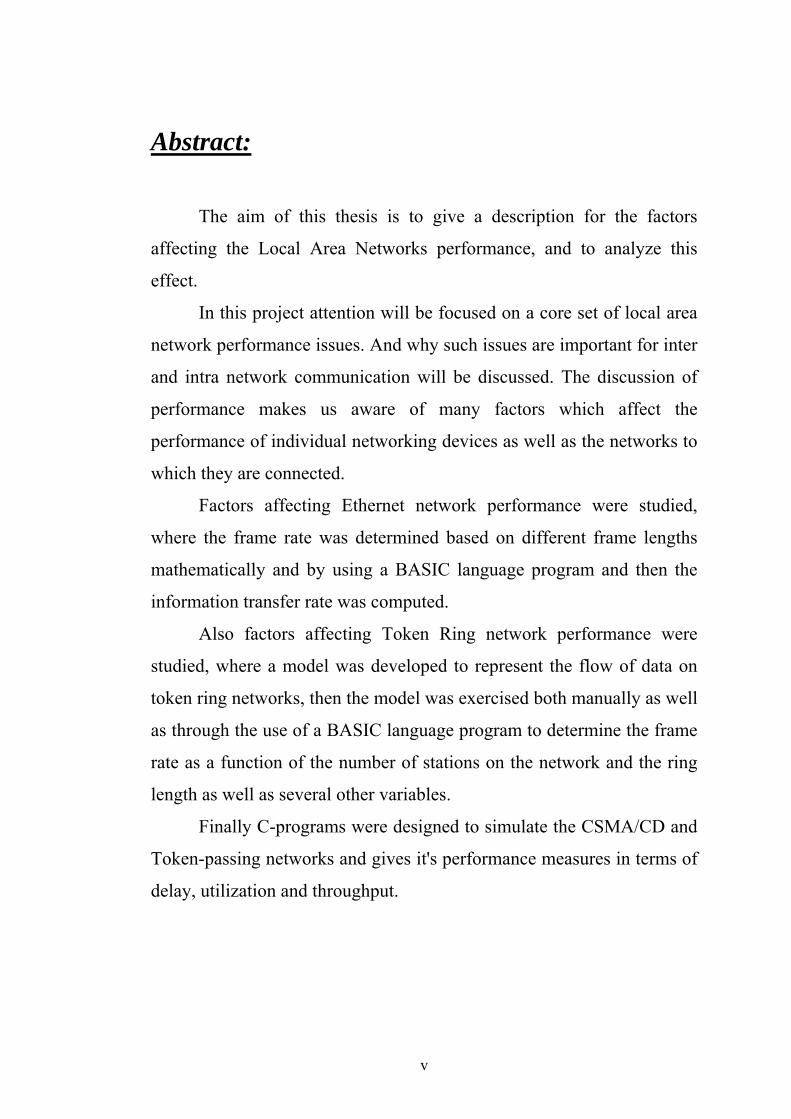
Abstract: The aim of this thesis is to give a description for the factors
affecting the Local Area Networks performance, and to analyze this
effect.
In this project attention will be focused on a core set of local area
network performance issues. And why such issues are important for inter
and intra network communication will be discussed. The discussion of
performance makes us aware of many factors which affect the
performance of individual networking devices as well as the networks to
which they are connected.
Factors affecting Ethernet network performance were studied,
where the frame rate was determined based on different frame lengths
mathematically and by using a BASIC language program and then the
information transfer rate was computed.
Also factors affecting Token Ring network performance were
studied, where a model was developed to represent the flow of data on
token ring networks, then the model was exercised both manually as well
as through the use of a BASIC language program to determine the frame
rate as a function of the number of stations on the network and the ring
length as well as several other variables.
Finally C-programs were designed to simulate the CSMA/CD and
Token-passing networks and gives it's performance measures in terms of
delay, utilization and throughput.
v

:المستخلص
ة شبكات المحلي اءة ال ى آف ؤثر عل الهدف من هذا المشروع عمل دراسة للعوامل التي ت
.وتحليل هذه المؤثرات
ة . في هذا المشروع سيتم الترآيز على صميم أداء الشبكات المحلية ومناقشة مامدى أهمي
لنا نلم بالعديد من مناقشة موضوع آفاءة الشبكات يجع . هذا الموضوع لعملية إتصال هذه الشبكات
.العوامل التي توثر على آفاءة أجهزة الشبكات والشبكات التي تعمل بها هذه الأجهزة
م حساب ، (Ethernet)تم عمل دراسة للعوامل التي تؤثر على شبكة الإيثرنت حيث ت
ز ، معدل عدد الفريمات عند تغير طول الفريم ة البي ك تم الحساب رياضياً وعن طريق برامج بلغ
(Basic)ومن ثم تم حساب معدل حرآة المعلومات .
ج وآن رن ى شبكة الت ؤثر عل ضاً عمل دراسة للعوامل التي ت م أي (Token Ring)وت
ار النموزج م إختب م ت حيث تم تصميم نموزج يمثل حرآة البيانات في شبكات التوآن رنج ومن ث
ر أي لمع (Basic)وعن طريق برامج بلغة البيزك ) رياضياً(يدوياً د تغي دل الفريمات عن رفة مع
.من عدد الحطات بالشبكة أو طول الشبكة بالإضافة لعوامل أخرى
ـ ة ال رامج بلغ صميم ب م ت راً ت ـ Cأخي بكات ال اة ش -Token و CSMA/CD لمحاآ
passingوإعطاء قياسات للكفاءة عن طريق قياس التاخير والإستخدام والإنتاجية .
vi

Chapter One
Introduction
Chapter One
Introduction
1.1 Overview:
Local Area Network (LAN) technology has made a significant
impact on almost every industry. Operations of these industries depend
on computers and networking. The data is stored on computers than on
paper, and the dependence on networking is so high that banks, airlines,
insurance companies and many government organizations would stop
functioning if there were a network failure. In our days the network
become like backbone of the most business and the base that a company
builds its work on.
Effective and meaningful interchange of information is an
essential element in the operation of enterprises and the conduct of
business activity. The dramatic advances in computer and
communication technology are now providing comprehensive
capabilities for the establishment of distributed information system fully
interconnected and integrated to serve as the foundation of business
around the world.
The field of computer networking is changing rapidly and entering
the exponential growth phase of its life cycle and it is becoming an
important part of every computer science curriculum. The enrollment in
networking courses at universities is growing exponentially just like the
number of networks that are being connected to the Internet.
1
1.2 Data Communication Networks:
The purpose of a computer communications network is to allow
moving information from one point to another inside the network. The
information could be stored on a device, such as a personal computer in
the network; it could be generated live outside the network, such as
speech, or could be generated by a process on another piece of
information, such as automatic sales transactions at the end of a business
day. The device does not necessarily have to be a computer; it could be a
hard disk, a camera or even a printer on the network. Due to a large
variety of information to be moved, and due to the fact that each type of
information has its own conditions for intelligibility, the computer
network has evolved into a highly complex system. Specialized
knowledge from many areas of science and engineering goes into the
design of networks. It is practically impossible for a single area of
science or engineering to be entirely responsible for the design of all the
components.
An important requirement of the information society is the facility
to transfer data to a remote location quickly and conveniently. The data
is transferred by means of telecommunication networks. By using a
network we can use computer terminals to do our tasks. The benefits of
these techniques due:
1. Sharing of files, documents, software and resources.
2. Sending massages to all users on the network.
2
1.3 Medium Access:
Medium Access is an effective methodology that allows devices
on a LAN to share their interconnecting media and due to the shared
nature of the media, it is obvious that more than one device might send
data at the same time, and it is classified as:
[1] Random Access: 1.1 ALOHA (Developed by University of Hawaii). 1.2 Slotted ALOHA. 1.3 Carrier Sense Multiple Access (CSMA). 1.4 Carrier Sense Multiple Access With Collision Detection
(CSMA/CD).
[2] Scheduling Medium Access: 2.1 Reservation System. 2.2 Polling. 2.3 Token Passing Rings.
[3] Channelization: 3.1 Frequency Division Multiple Access (FDMA). 3.2 Time Division Multiple Access (TDMA). 3.3 Code Division Multiple Access (CDMA).
1.4 What is performance? The words that network administrators hate to hear are “The
network seems slow today.” What exactly is a slow network, and how
can you tell? Who determines when the network is slow, and how do
they do it? There are usually more questions than answers when you’re
dealing with network performance in a production network environment.
It would be great if there were standard answers to these
questions, along with a standard way to solve slow network
performance. Often, network bottlenecks can be found, and simply
reallocating the resources on a network can greatly improve
3
performance, without the addition of expensive new network equipment.
1.5 Measures of Performance:
Network performance is a complex issue, with lots of independent
variables that affect it. However, most of the elements involved in the
performance of networks can be boiled down to a few simple network
principles that can be measured, monitored, and controlled.
There are three common measures of LAN Performance:
1. Delay (D): Which occurs between the time a packet or a frame is
ready for transmission from a node, and the completion of
successful transmission.
2. Throughput (S): The total rate of data being transmitted between
nodes (carried load) in bit/second and it is expressed as a fraction
of capacity.
3. Utilization (U): The fraction of total capacity being used.
Factors Affecting Performance: The performance of a network depends on a number of factors the most important are:
1. Data rate (Transmission Rate). 2. Propagation Time. 3. Transmission Time 4. Frame size (Number of bits per frame). 5. Local Network Protocols (MAC Protocol). 6. Offered Load. 7. Number of stations. 8. Jitter. 9. Topology. 10. Error rate.
4
1.6 Objective:
The aim of this project is to know the factors that affect
performance and the relative performance of various local network
schemes, and to present analytic techniques that can be used for network
sizing and to obtain first approximations of network performance, and
design simulation programs to calculate and measure the performance of
LAN.
1.7 Thesis layout:
This thesis is composed of seven chapters; the outlines of these chapters
are as follows:
• Chapter Two, provides a brief review of local area networks as
definitions of LAN and it is topologies and how different LANs
work.
• Chapter Three, consider how fast can frames flow on an Ethernet
network, and it focuses attention on the Carrier Sense Multiple
Access with Collision Detection (CSMA/CD) network access
protocol. By closely examining this protocol, we can determine
the maximum frame rate that can be supported on a 10 Mbps, 100
Mbps, and even 1 Gbps Ethernet networks based upon different
frame lengths.
• Chapter Four, the question previously asked concerning how fast
frames can flow on an Ethernet network is also applicable to
Token Ring networks. That is, if we can determine the flow of
information on a Token Ring network, we can use this information
to estimate the performance of the network as additional stations
are added to the network. By determining the frame flow on a
Token Ring network, we used this information to develop a model
5
• to project network and inter-LAN transmission time. So the focus
of chapter four is on the development of a model to reflect the
flow of frames on a Token Ring network, and this model was
exercised to determine the frame carrying capacity of a Token
Ring network under different operating conditions and network
configurations. Where a large number of operating conditions and
network configuration data were used. Some of the parameters
that had a bearing on the flow of frames on a Token Ring network
include the number of stations on the network, the length of each
lobe and the length of the ring, the average frame size, and the
operating rate of the network
• In chapter five, we discussed the simulation of CSMA/CD-based
local area networks. We present a step-by-step process of
simulating this type of LAN. A simulation program is also
described in detail, from providing input parameters to printing
output results. The output results are presented in terms of the
average delay per packet, the average throughput, the average
utilization, and the average collision rate
• Chapter six, we discussed the simulation of token-passing ring and
bus local area networks. We have explained a simulation program
step by step that takes the input parameters from the user and
simulates one of the LANs at a time to a desired level of
convergence.
• Chapter seven, where we gives a conclusion what we have done
and gives recommendations for future work.
6
Chapter Two
Local Area Networks

Chapter Two Local Area Networks
In order to fully participate in the information age, one must be
able to communicate with others in a multitude of ways. However, the
greatest interest today is centered on computer generated data, and its
transmission has become the most rapidly developing facet of the
communication industry. The overall communication problem may be
viewed as involving three types of networks:
• Local area networks (LANs) providing communications over a
relatively small area
• Metropolitan area networks (MANs) operating over a few hundred
kilometers
• Wide area networks (WANs) providing communications over several
kilometers (thousandth), across the nation, or around the globe
Although the three types of communication networks employ
identical principles, their characteristics are quite different. In a WAN,
which may span continents, the transmission media are relatively
expensive because of the large extent of the networks. Transmission
rates in a WAN may range from 2,400 to about 50,000 bits per second,
whereas in a LAN they are much higher, typically from 10 to 1000
million bits per second. In a WAN, the data arrival rate is low enough to
permit processors to ensure error-free transmission and message
integrity. This is not the case with a LAN because of its much higher
data rate.
7
2.1 Definition of a LAN:
A LAN is a data communication system, usually owned by a
single organization that allows similar or dissimilar digital devices to
connect to each other over a common transmission medium. According
to the IEEE [1],
A local area network is distinguished from other types of data networks in that communication is usually confined to a moderate geographic area such as a single office building, a warehouse, or a campus, and can depend on a physical communications channel of moderate-to-high data rate which has a consistently low error rate.
Thus we may regard a LAN as a resource-sharing data
communication network with the following characteristics:
• Short distances (0.1 to 10 km)
• High speed (1 to 1000 Mbps)
• Low cost.
• Low error rate (10-8 to 10-11)
• Ease of access
• High reliability/integrity.
The network may connect data devices such as computers, terminals,
mass storage devices, and printers/plotters. Through the network these
devices can interchange data information such as file transfer, electronic
mail, and word processing.
8
2.2 Evolution of LANs:
LANs, as data communication networks, resulted from the
combining of two different technologies: telecommunications and
computers. Recent developments of large scale and very large scale (LSI
and VLSI) integrated circuits have rapidly reduced the cost of
computation and memory hardware. This has resulted in widely
available low-cost personal computers, intelligent terminals,
workstations, and minicomputers. However, other expensive resources
such as high-quality printers, graphic plotters, and disk storage are best
shared in a geographically limited area using a LAN.
Research in LANs began in the early 1970s, spurred by increasing
requirements for resource sharing in multiple processor environments.
Ethernet, the first bus contention technology, originated at Xerox
Corporation’s Palo Alto Research Center, in the mid-1970s. Called
Ethernet after the concept in classical physics of wave transmission
through an ether, the design borrowed many of the techniques and
characteristics of the Aloha network, a packet radio network developed
at the University of Hawaii. Since the introduction of Ethernet, networks
using a number of topologies and protocols have been developed and
reported.
LANs represent a comparatively new field of activity and continue
to hold the public interest. This is mirrored by the numerous courses
being offered in the subject, by the many conference sessions devoted to
LANs, by the research and development work on LANs being pursued
both at the universities and in industries, and by the increasing amount of
literature devoted to LANs.
9
All this interest is generated by the LAN’s promise as a means of
interconnecting various computers or computer-related devices into
systems that are more useful than their individual parts. The goal of
LANs is to provide a large number of devices with inexpensive yet high-
speed local communications.
Communication between computers is becoming increasingly
important as data processing becomes a commodity. Local area
networking is a very rapidly growing field. Continued efforts are being
made for further technological developments and innovations in the
organization of these networks for maximal operational efficiency.
2.3 LAN Technology:
The types of technologies used to implement LANs are diverse.
Both vendors and users are compelled to make a choice. This choice is
usually based on several criteria such as:
• Network topology and architecture
• Access control
• Transmission medium
• Transmission technique
• Adherence to standards
• Performance in terms of channel utilization, delay, power, and
effective transmission ratio.
The first four criteria are the major technological issues and are of
great concern when discussing LANs. These issues are sometimes
10
interrelated. For example, some access methods are only suitable for
some topologies or with certain transmission techniques.
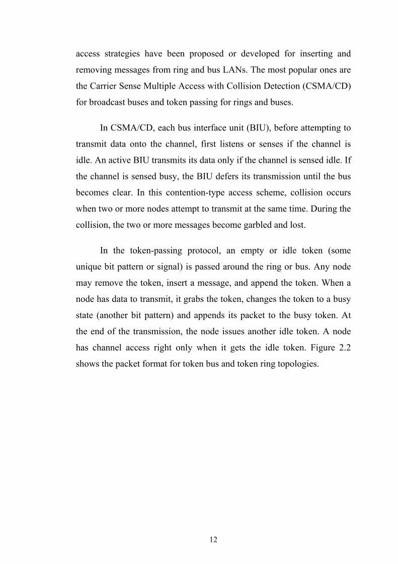
2.3.1 Network Topology and Access Control:
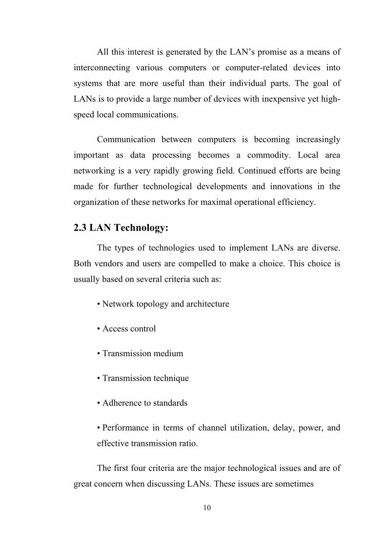
The topology of a network is the way in which the nodes (or
stations) are interconnected (The basic forms of the topologies are shown
in Figure 2.1).
Figure 2.1 Local network topologies.
In the ring topology, all nodes are connected together in a closed
loop. Information passes from node to node on the loop and is
regenerated (by repeaters) at each node (called an active interface). A
bus topology uses a single, open-ended transmission medium. Each node
taps into the medium in a way that does not disturb the signal on the bus
(thus it is called a passive interface). Star topology consists of a central
controlling node with star-like connections to various other nodes.
Both ring and bus topologies, lacking any central node, must use
some distributed mechanism to determine which node may use the
transmission medium at any given moment. Various flow control and
11
access strategies have been proposed or developed for inserting and
removing messages from ring and bus LANs. The most popular ones are
the Carrier Sense Multiple Access with Collision Detection (CSMA/CD)
for broadcast buses and token passing for rings and buses.
In CSMA/CD, each bus interface unit (BIU), before attempting to
transmit data onto the channel, first listens or senses if the channel is
idle. An active BIU transmits its data only if the channel is sensed idle. If
the channel is sensed busy, the BIU defers its transmission until the bus
becomes clear. In this contention-type access scheme, collision occurs
when two or more nodes attempt to transmit at the same time. During the
collision, the two or more messages become garbled and lost.
In the token-passing protocol, an empty or idle token (some
unique bit pattern or signal) is passed around the ring or bus. Any node
may remove the token, insert a message, and append the token. When a
node has data to transmit, it grabs the token, changes the token to a busy
state (another bit pattern) and appends its packet to the busy token. At
the end of the transmission, the node issues another idle token. A node
has channel access right only when it gets the idle token. Figure 2.2
shows the packet format for token bus and token ring topologies.
12
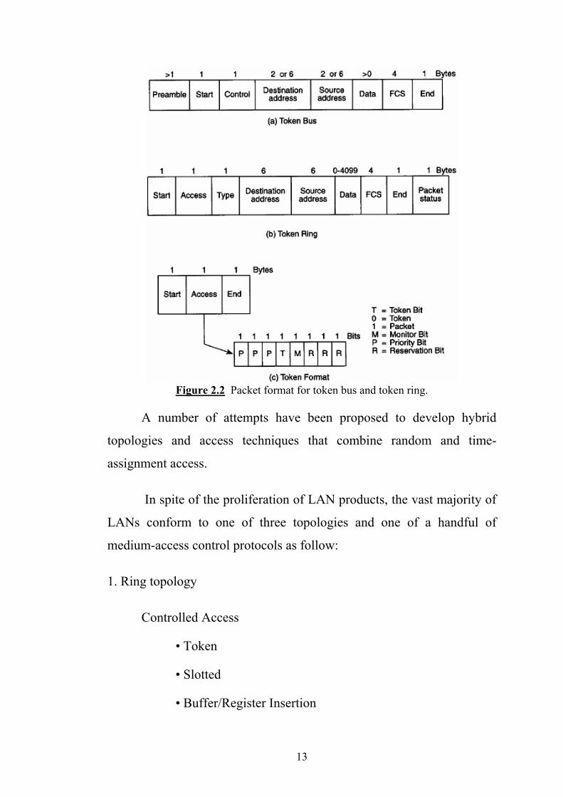
Figure 2.2 Packet format for token bus and token ring.
A number of attempts have been proposed to develop hybrid
topologies and access techniques that combine random and time-
assignment access.
In spite of the proliferation of LAN products, the vast majority of
LANs conform to one of three topologies and one of a handful of
medium-access control protocols as follow:
1. Ring topology
Controlled Access
• Token
• Slotted
• Buffer/Register Insertion
13
2. Bus topology
Controlled Access
• Token
• Multilevel Multiple Access (MLMA)
Random Access
• Carrier Sense Multiple Access (CSMA) (1-persistent, p-
persistent, nonpersistent).
• Carrier Sense Multiple Access with Collision Detection
(CSMA/CD).
• CSMA/CD with Dynamic Priorities (CSMA/CD-DP)
• CSMA/CD with Deterministic Contention Resolution
(CSMA/CD-DCR)
3. Star topology
Random Access
• Carrier Sense Multiple Access (CSMA) (1-persistent, p-
persistent, nonpersistent).
• Carrier Sense Multiple Access with Collision Detection
(CSMA/CD).
• CSMA/CD with Dynamic Priorities (CSMA/CD-DP)
• CSMA/CD with Deterministic Contention Resolution
(CSMA/CD-DCR)
14
4. Hybrid topology
• Ring-star
• Ring-bus
• Bus-star
2.3.2 Transmission Media
The transmission medium is the physical path connecting the
transmitter to the receiver. Any physical medium that is capable of
carrying information in an electromagnetic form is potentially suitable
for use on a LAN. In practice, the media used are twisted-pair cable,
coaxial cable, and optical fiber.
Twisted-pair cable comes in two varieties: shielded and
unshielded. Unshielded twisted pair (UTP) is the most popular and is
generally the best option for small LANs because it is thin, flexible and
easily used. Also, it is cheap.
Coaxial cable is highly resistant to signal interference. So it can
support greater cable lengths between network devices than twisted pair
cable.
Fiber optic cable has the ability to transmit signals over much
longer distances than coaxial and twisted pair. It also has the capability
to carry information at high speed.
15
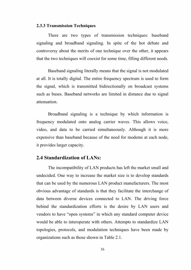
2.3.3 Transmission Techniques
There are two types of transmission techniques: baseband
signaling and broadband signaling. In spite of the hot debate and
controversy about the merits of one technique over the other, it appears
that the two techniques will coexist for some time, filling different needs.
Baseband signaling literally means that the signal is not modulated
at all. It is totally digital. The entire frequency spectrum is used to form
the signal, which is transmitted bidirectionally on broadcast systems
such as buses. Baseband networks are limited in distance due to signal
attenuation.
Broadband signaling is a technique by which information is
frequency modulated onto analog carrier waves. This allows voice,
video, and data to be carried simultaneously. Although it is more
expensive than baseband because of the need for modems at each node,
it provides larger capacity.
2.4 Standardization of LANs:
The incompatibility of LAN products has left the market small and
undecided. One way to increase the market size is to develop standards
that can be used by the numerous LAN product manufacturers. The most
obvious advantage of standards is that they facilitate the interchange of
data between diverse devices connected to LAN. The driving force
behind the standardization efforts is the desire by LAN users and
vendors to have “open systems” in which any standard computer device
would be able to interoperate with others. Attempts to standardize LAN
topologies, protocols, and modulation techniques have been made by
organizations such as those shown in Table 2.1.
16
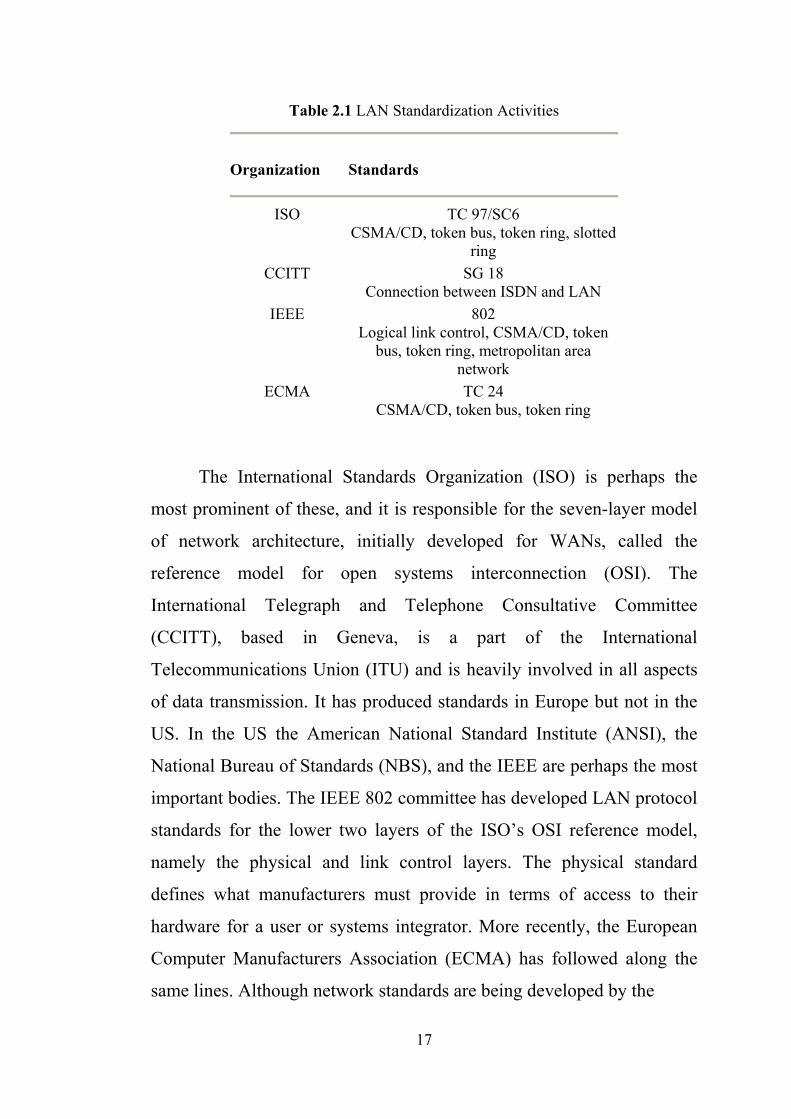
Table 2.1 LAN Standardization Activities
Organization Standards
ISO TC 97/SC6
CSMA/CD, token bus, token ring, slotted ring
CCITT SG 18 Connection between ISDN and LAN
IEEE 802 Logical link control, CSMA/CD, token
bus, token ring, metropolitan area network
ECMA TC 24 CSMA/CD, token bus, token ring
The International Standards Organization (ISO) is perhaps the
most prominent of these, and it is responsible for the seven-layer model
of network architecture, initially developed for WANs, called the
reference model for open systems interconnection (OSI). The
International Telegraph and Telephone Consultative Committee
(CCITT), based in Geneva, is a part of the International
Telecommunications Union (ITU) and is heavily involved in all aspects
of data transmission. It has produced standards in Europe but not in the
US. In the US the American National Standard Institute (ANSI), the
National Bureau of Standards (NBS), and the IEEE are perhaps the most
important bodies. The IEEE 802 committee has developed LAN protocol
standards for the lower two layers of the ISO’s OSI reference model,
namely the physical and link control layers. The physical standard
defines what manufacturers must provide in terms of access to their
hardware for a user or systems integrator. More recently, the European
Computer Manufacturers Association (ECMA) has followed along the
same lines. Although network standards are being developed by the
17
various organizations, standardization is still up to the manufacturers.
The ISO protocols have the advantage of international backing, and most
manufacturers have made the commitment to implement them
eventually.
2.5 LAN Architectures:
Network architecture is a specification of the set of functions
required for a user at a location to interact with another user at another
location. These interconnect functions include determination of the start
and end of a message, recognition of a message address, management of
a communication link, detection and recovery of transmission errors, and
reliable and regulated delivery of data. General network architecture thus
describes the interfaces, algorithms, and protocols by which processes at
different locations and/or at heterogeneous machines could
communicate. Although the architectures developed by different vendors
are functionally equivalent, they do not provide for easy interconnection
of systems of different make.
2.5.1 The OSI Model
As mentioned in the previous section, the need for standardization
and compatibility at all levels has compelled the International Standards
Organization (ISO) to establish a general seven-layer hierarchical model
for universal intercomputer communication. This architecture, known as
the Open Systems Interconnection model (see Figure 2.3), defines seven
layers of communication protocols, with specific functions isolated at
each level. The OSI model is a reference model for the exchange of
information among systems that are open to one another for this purpose
by virtue of their mutual use of the applicable standards.
18
The seven hierarchical layers are hardware and software
functional groupings with specific well-defined tasks. The OSI model
states the purpose of each layer and describes the services provided by
each within its layer and to the adjacent higher and lower layers. Details
of the implementation of each layer of OSI model depend on the
specifics of the application and the characteristics of the communication
channel employed.
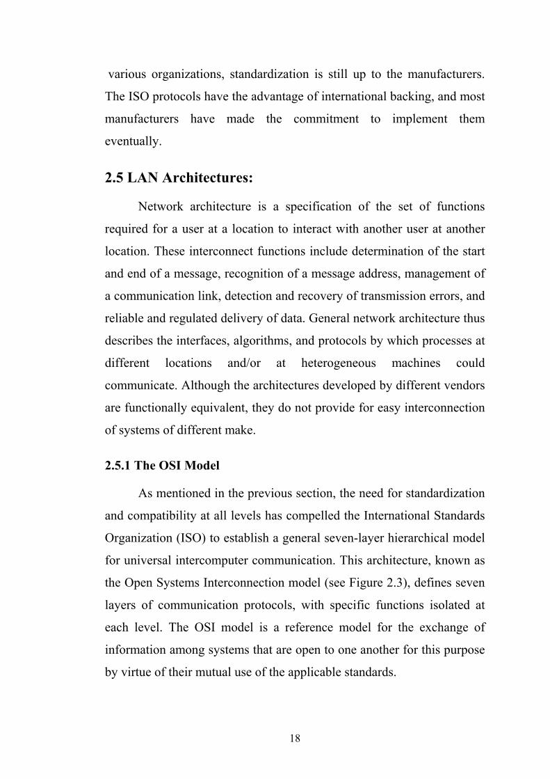
Figure 2.3 Relationship between the OSI model and IEEE LAN layers.
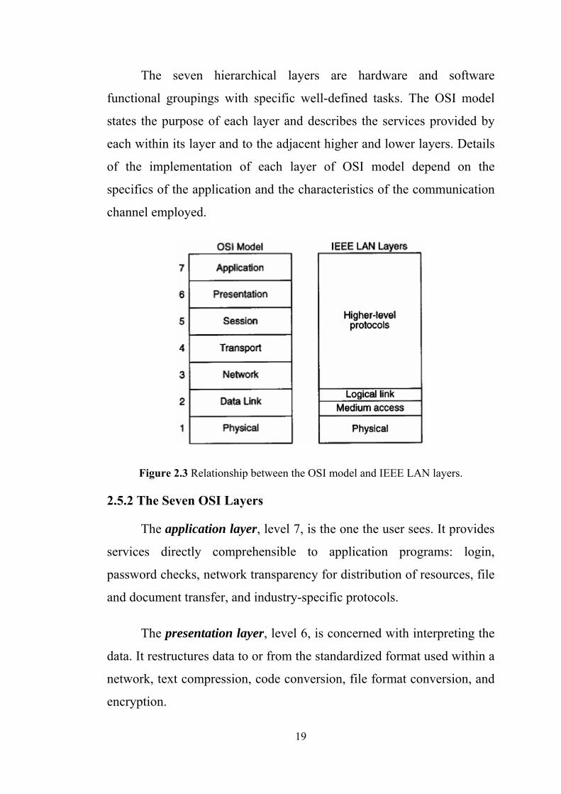
2.5.2 The Seven OSI Layers
The application layer, level 7, is the one the user sees. It provides
services directly comprehensible to application programs: login,
password checks, network transparency for distribution of resources, file
and document transfer, and industry-specific protocols.
The presentation layer, level 6, is concerned with interpreting the
data. It restructures data to or from the standardized format used within a
network, text compression, code conversion, file format conversion, and
encryption.
19
The session layer, level 5, manages address translation and access
security. It negotiates to establish a connection with another node on the
network and then to manage the dialogue. This means controlling the
starting, stopping, and synchronization of the conversion.
The transport layer, level 4, performs error control, sequence
checking, handling of duplicate packets, flow control, and multiplexing.
Here it is determined whether the channel is to be point-to-point (virtual)
with ordered messages, isolated messages with no order, or broadcast
messages. It is the last of the layers concerned with communications
between peer entities in the systems. The transport layer and those above
are referred to as the upper layers of the model, and they are independent
of the underlying network. The lower layers are concerned with data
transfer across the network.
The network layer, level 3, provides a connection path between
systems, including the case where intermediate nodes are involved. It
deals with message packetization, message routing for data transfer
between nonadjacent nodes or stations, congestion control, and
accounting.
The data link layer, level 2, establishes the transmission protocol,
how information will be transmitted, acknowledgment of messages,
token possession, error detection, and sequencing. It prepares the packets
passed down from the network layer for transmission on the network. It
takes a raw transmission and transforms it into a line free from error.
Here headers and framing information are added or removed. With these
go the timing signals, check-sum, and station addresses, as well as the
control system for access.
20
The physical layer, level 1, is that part that actually touches the
transmission medium or cable; the line is the point within the node or
device where the data is received and transmitted. It ensures that ones
arrive as ones and zeros as zeros. It encodes and physically transfers
messages (raw bits in a stream) between adjacent stations. It handles
voltages, frequencies, direction, pin numbers, modulation techniques,
signaling schemes, ground loop prevention, and collision detection in the
CSMA/CD access method.
2.5.3 The IEEE Model for LANs
The IEEE has formulated standards for the physical and logical
link layers for three types of LANs, namely, token buses, token rings,
and CSMA/CD protocols. Figure 2.3 illustrates the correspondence
between the three layers of the OSI and the IEEE 802 reference models.
The physical layer specifies means for transmitting and receiving bits
across various types of media. The media-access-control layer performs
the functions needed to control access to the physical medium. The
logical-link-control layer is the common interface to the higher software
layers.
2.6 Performance Evaluation:
In this section, we present simple performance models of LANs.
The performance is measured in terms of channel utilization, throughput
and delay.
2.6.1 Channel Utilization
A performance yardstick is the maximum throughput achievable
for a given channel capacity. For example, how many megabits per
21
second (Mbps) of data can actually be transmitted for a channel capacity
of 10 Mbps? It is certain that a fraction of the channel capacity is used up
in form of overhead, acknowledgments, retransmission, token delay, etc.
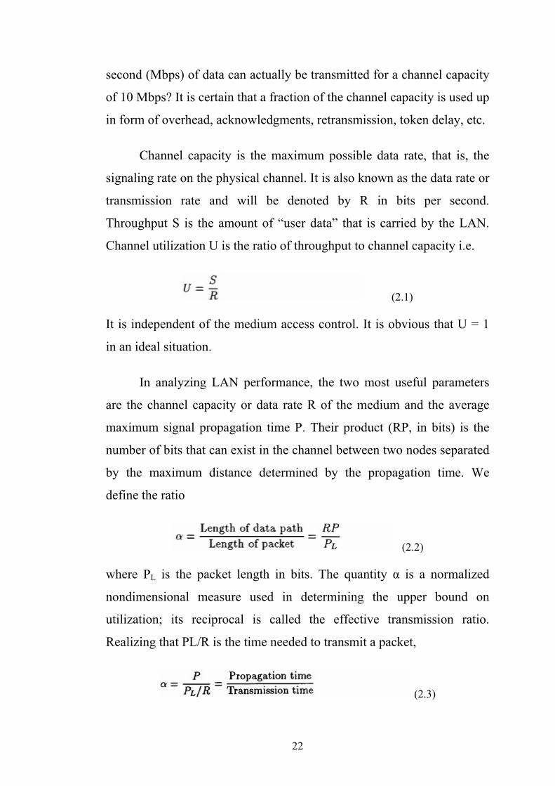
Channel capacity is the maximum possible data rate, that is, the
signaling rate on the physical channel. It is also known as the data rate or
transmission rate and will be denoted by R in bits per second.
Throughput S is the amount of “user data” that is carried by the LAN.
Channel utilization U is the ratio of throughput to channel capacity i.e.
(2.1)
It is independent of the medium access control. It is obvious that U = 1
in an ideal situation.
In analyzing LAN performance, the two most useful parameters
are the channel capacity or data rate R of the medium and the average
maximum signal propagation time P. Their product (RP, in bits) is the
number of bits that can exist in the channel between two nodes separated
by the maximum distance determined by the propagation time. We
define the ratio
(2.2)
where PL is the packet length in bits. The quantity α is a normalized
nondimensional measure used in determining the upper bound on
utilization; its reciprocal is called the effective transmission ratio.
Realizing that PL/R is the time needed to transmit a packet,
(2.3)
22
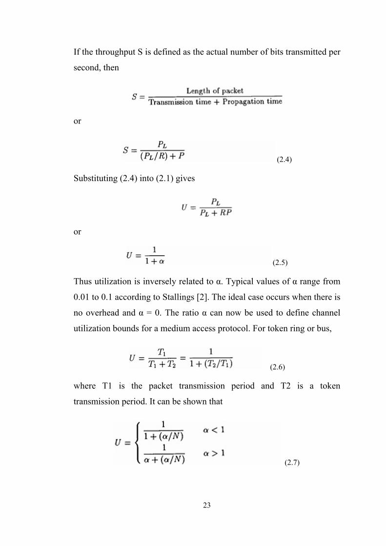
If the throughput S is defined as the actual number of bits transmitted per
second, then
or
(2.4)
Substituting (2.4) into (2.1) gives
or
(2.5)
Thus utilization is inversely related to α. Typical values of α range from
0.01 to 0.1 according to Stallings [2]. The ideal case occurs when there is
no overhead and α = 0. The ratio α can now be used to define channel
utilization bounds for a medium access protocol. For token ring or bus,
(2.6)
where T1 is the packet transmission period and T2 is a token
transmission period. It can be shown that
(2.7)
23
where N is the number of active nodes or stations. In a token bus, the
optimal case occurs when the logical ordering of nodes is the same as the
physical order. In this case, Eq. (2.7) applies. In the worst case, the
logical ordering of nodes forces the propagation delay between nodes to
approach the end-to-end delay. For this case, T2 = α and
(2.8)
2.6.2 Delay:
Packet delay is the period of time between the moment at which a
node becomes active (i.e., when it has data to transmit) and the moment at
which the packet is successfully transmitted. Throughput delay describes the
trade-off between throughput and packet delay. Delay D is the sum of the
service time S plus the time W spent waiting to transmit all messages queued
ahead of it and the actual propagation delay Tp. Thus
(2.9)
24
Chapter Three
Factors Affecting Ethernet Network Performance
Chapter Three
Factors Affecting Ethernet Network Performance
In this chapter we begin to focus attention on the performance
requirements of specific types of LANs by examining the CSMA/CD
access protocol. This will enable us to construct a model that reflects the
transfer of frames on Ethernet, Fast Ethernet, and Gigabit Ethernet
networks at different levels of network utilization. This, in turn, will
provide us with a foundation for computing the maximum frame
forwarding rate required to be supported by a bridge, router, or switch
connected to an Ethernet network to ensure the device is fully capable of
supporting the maximum level of Ethernet transmission.
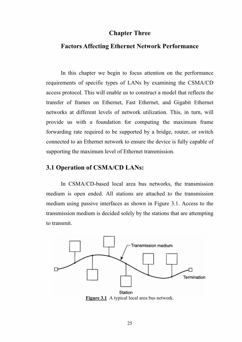
3.1 Operation of CSMA/CD LANs:
In CSMA/CD-based local area bus networks, the transmission
medium is open ended. All stations are attached to the transmission
medium using passive interfaces as shown in Figure 3.1. Access to the
transmission medium is decided solely by the stations that are attempting
to transmit.
Figure 3.1 A typical local area bus network.
25
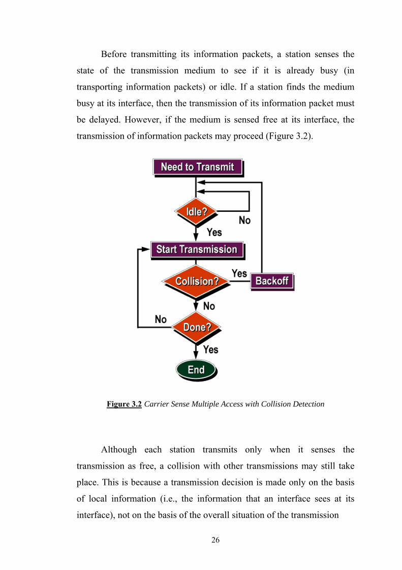
Before transmitting its information packets, a station senses the
state of the transmission medium to see if it is already busy (in
transporting information packets) or idle. If a station finds the medium
busy at its interface, then the transmission of its information packet must
be delayed. However, if the medium is sensed free at its interface, the
transmission of information packets may proceed (Figure 3.2).
Figure 3.2 Carrier Sense Multiple Access with Collision Detection
Although each station transmits only when it senses the
transmission as free, a collision with other transmissions may still take
place. This is because a transmission decision is made only on the basis
of local information (i.e., the information that an interface sees at its
interface), not on the basis of the overall situation of the transmission
26
medium. When a station transmits its packets, it takes a small but finite
amount of time (end-to-end propagation delay τ seconds, in the worst
case) before this information reaches all stations. Consider a situation in
which a station senses the transmission medium at its interface as free
and begins its transmission. Another station senses the transmission
medium at its interface as free because the previous station’s
transmission has not reached its interface yet, so this station also begins
its transmission. Now two transmissions are in progress at the same time
and will definitely collide within τ seconds.
During transmission of their information packets, all stations
monitor transmitted information packets on the transmission medium.
The information on the medium is compared with what each station is
transmitting. If these two match then it is assumed that the transmission
is successful. However, if the transmitted information differs from what
is on the transmission medium, it is assumed that a collision has taken
place and a retransmission is needed.
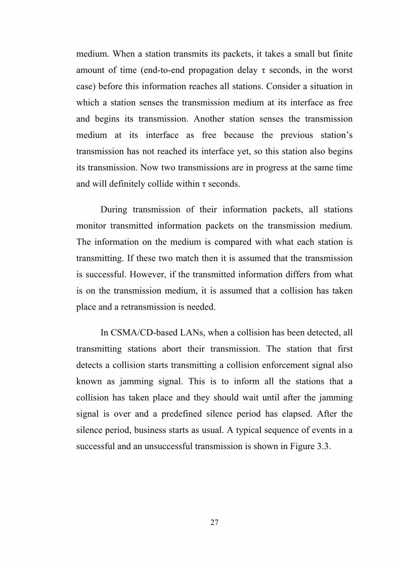
In CSMA/CD-based LANs, when a collision has been detected, all
transmitting stations abort their transmission. The station that first
detects a collision starts transmitting a collision enforcement signal also
known as jamming signal. This is to inform all the stations that a
collision has taken place and they should wait until after the jamming
signal is over and a predefined silence period has elapsed. After the
silence period, business starts as usual. A typical sequence of events in a
successful and an unsuccessful transmission is shown in Figure 3.3.
27
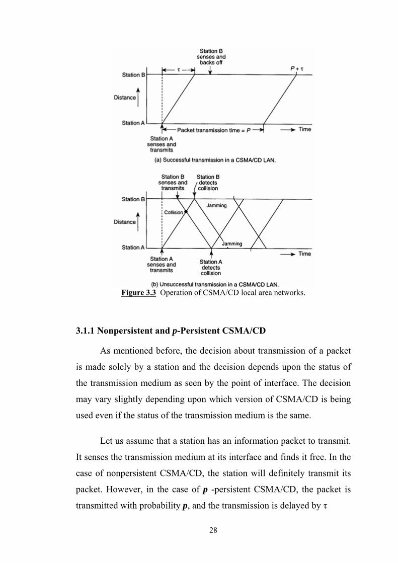
Figure 3.3 Operation of CSMA/CD local area networks.
3.1.1 Nonpersistent and p-Persistent CSMA/CD
As mentioned before, the decision about transmission of a packet
is made solely by a station and the decision depends upon the status of
the transmission medium as seen by the point of interface. The decision
may vary slightly depending upon which version of CSMA/CD is being
used even if the status of the transmission medium is the same.
Let us assume that a station has an information packet to transmit.
It senses the transmission medium at its interface and finds it free. In the
case of nonpersistent CSMA/CD, the station will definitely transmit its
packet. However, in the case of p -persistent CSMA/CD, the packet is
transmitted with probability p, and the transmission is delayed by τ
28
seconds (end-to- end propagation delay) with probability (1 - p). If p
happens to equal 1, as is the case in Ethernet implementations, the packet
will also be transmitted immediately after the transmission medium is
sensed free.
On the other hand, if the transmission medium is sensed busy, no
packet should be transmitted. In the case of nonpersistent CSMA/CD,
the station backs off and senses the transmission medium again after a
random duration of time. In the case of p -persistent CSMA/CD, the
station keeps on checking the transmission medium continuously until it
becomes free. As soon as the medium becomes free, the station transmits
its packet with probability p and delays it by τ seconds with probability
(1 - p). Obviously, if p = 1 in the p -persistent case, the station will
immediately transmit after the transmission medium becomes free. In
this case, if more than one station was checking the transmission
medium at the same time, all of them will transmit almost at the same
time and will collide with probability 1.
So it is simple to calculate the performance of a CSMA/CD
network where only one node attempts to transmit at any time. In this
case, the NIC (Network Interface Card) may saturate the medium and
near 100% utilization of the link may be achieved, providing almost 10
Mbps of throughput on a 10 Mbps LAN.
However, when two or more NICs attempt to transmit at the same
time, the performance of Ethernet is less predictable. The fall in
utilization and throughput occurs because some bandwidth is wasted by
collisions and back-off delays. In practice, a busy shared 10 Mbps
Ethernet network will typically supply 2-4 Mbps of throughput to the
NICs connected to it.
29
As the level of utilization of the network increases, particularly if
there are many NICs competing to share the bandwidth, an overload
condition may occur. In this case, the throughput of Ethernet LANs
reduces very considerably, and much of the capacity is wasted by the
CSMA/CD algorithm, and very little is available for sending useful data.
This is the reason why a shared Ethernet LAN should not connect more
than 1024 computers [8]. Figure 3.4 shows the computed throughput
versus offered traffic for all three protocols, as well as for pure and
slotted ALOHA.
Figure 3.4 Comparison of the channel utilization versus load for various random
access protocols.
3.2. Determining the Network Frame Rate
In this section we compute the frame rate on Ethernet, 100BASE-
TX Fast Ethernet, and Gigabit Ethernet networks. We compute the frame
rate on 10 Mbps Ethernet, we will simply multiply the result by 10 to
determine the frame rate on Fast Ethernet, and by 100 to determine the
frame rate on Gigabit Ethernet (Gigabit Ethernet requires carrier
extension technology to insure the transmission of a minimum length
frame).
30
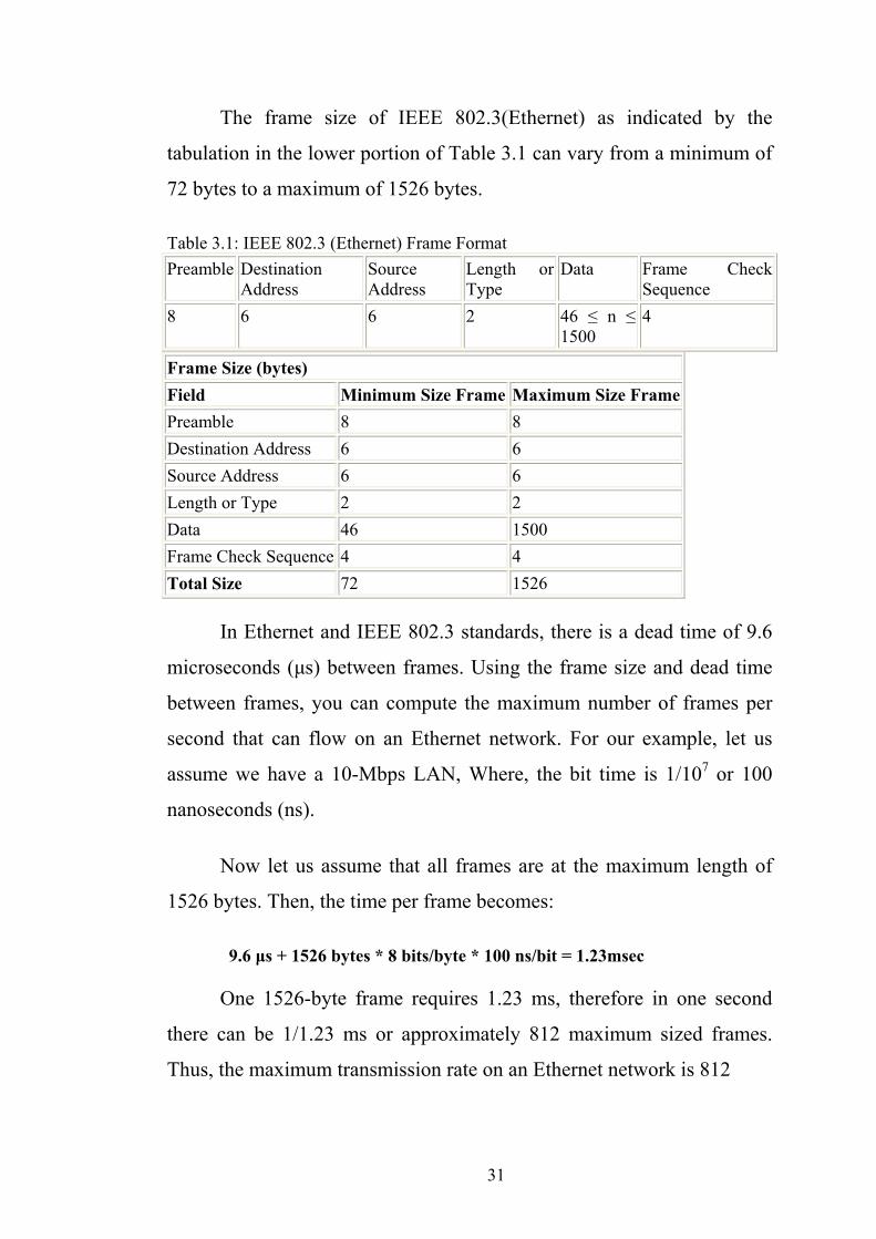
The frame size of IEEE 802.3(Ethernet) as indicated by the
tabulation in the lower portion of Table 3.1 can vary from a minimum of
72 bytes to a maximum of 1526 bytes.
Table 3.1: IEEE 802.3 (Ethernet) Frame Format Preamble Destination
Address Source Address
Length or Type
Data Frame Check Sequence
8 6 6 2 46 ≤ n ≤ 1500
4
Frame Size (bytes) Field Minimum Size Frame Maximum Size Frame Preamble 8 8 Destination Address 6 6 Source Address 6 6 Length or Type 2 2 Data 46 1500 Frame Check Sequence 4 4 Total Size 72 1526
In Ethernet and IEEE 802.3 standards, there is a dead time of 9.6
microseconds (µs) between frames. Using the frame size and dead time
between frames, you can compute the maximum number of frames per
second that can flow on an Ethernet network. For our example, let us
assume we have a 10-Mbps LAN, Where, the bit time is 1/107 or 100
nanoseconds (ns).
Now let us assume that all frames are at the maximum length of
1526 bytes. Then, the time per frame becomes:
9.6 µs + 1526 bytes * 8 bits/byte * 100 ns/bit = 1.23msec
One 1526-byte frame requires 1.23 ms, therefore in one second
there can be 1/1.23 ms or approximately 812 maximum sized frames.
Thus, the maximum transmission rate on an Ethernet network is 812
31
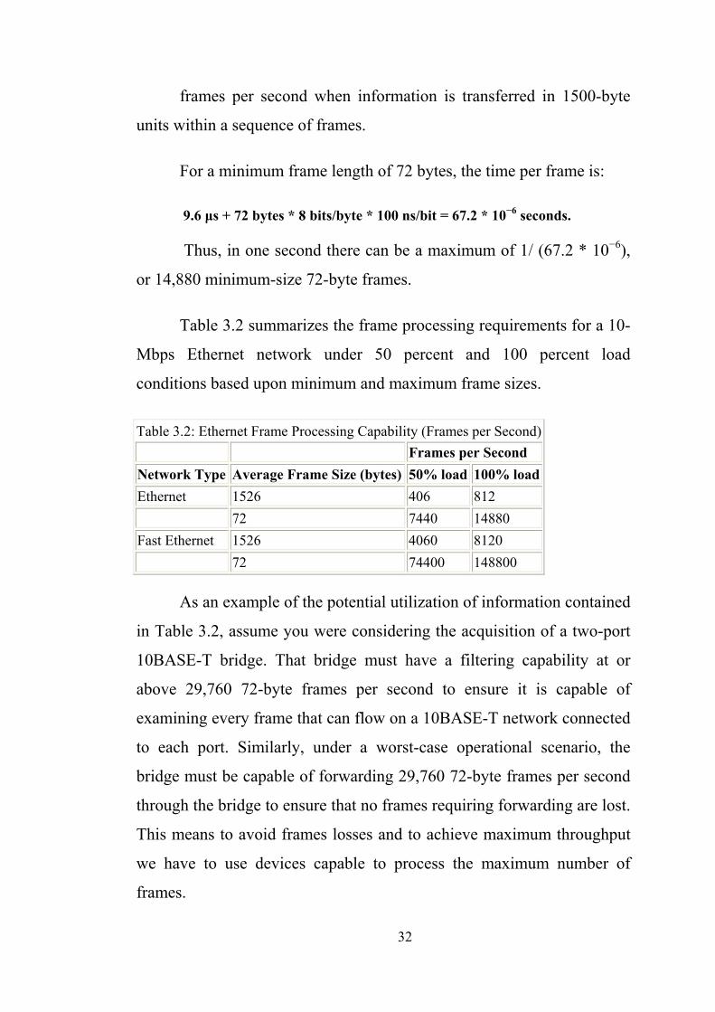
frames per second when information is transferred in 1500-byte
units within a sequence of frames.
For a minimum frame length of 72 bytes, the time per frame is:
9.6 µs + 72 bytes * 8 bits/byte * 100 ns/bit = 67.2 * 10−6 seconds.
Thus, in one second there can be a maximum of 1/ (67.2 * 10−6),
or 14,880 minimum-size 72-byte frames.
Table 3.2 summarizes the frame processing requirements for a 10-
Mbps Ethernet network under 50 percent and 100 percent load
conditions based upon minimum and maximum frame sizes.
Table 3.2: Ethernet Frame Processing Capability (Frames per Second) Frames per Second Network Type Average Frame Size (bytes) 50% load 100% load Ethernet 1526 406 812 72 7440 14880 Fast Ethernet 1526 4060 8120 72 74400 148800
As an example of the potential utilization of information contained
in Table 3.2, assume you were considering the acquisition of a two-port
10BASE-T bridge. That bridge must have a filtering capability at or
above 29,760 72-byte frames per second to ensure it is capable of
examining every frame that can flow on a 10BASE-T network connected
to each port. Similarly, under a worst-case operational scenario, the
bridge must be capable of forwarding 29,760 72-byte frames per second
through the bridge to ensure that no frames requiring forwarding are lost.
This means to avoid frames losses and to achieve maximum throughput
we have to use devices capable to process the maximum number of
frames.
32
3.2.1 Gigabit Ethernet Considerations
Gigabit Ethernet uses carrier extension technology to ensure that
the minimum length frame is 512 bytes, not including its preamble and
start of frame delimiter (SFD) fields.
The carrier extension field will vary in length from a maximum of
448 bytes when a minimum-length 64-byte frame is formed, to 0 bytes
when a frame with an information field equal to or greater than 494 bytes
in length is transmitted. Note that the actual frame length flowing on the
media includes preamble and SFD fields, requiring a minimum length
frame of 520 bytes for Gigabit Ethernet.
For a Gigabit Ethernet minimum length frame of 520 bytes, the
time per frame computations use a dead time of 0.096 µs between frames
and a bit duration of 1 ns. Thus, for a minimum frame length of 520
bytes, the time per frame becomes:
0.096 µs + 520 bytes * 8 bits/byte * 1 ns/bit = 4.256 µs
Then, in one second, there can be a maximum of 1/4.256 µs or
234,962 minimum-size 520-byte frames. To compute the maximum
number of maximum length frames that can flow on a Gigabit Ethernet
network, we would use a frame length of 1526 bytes, to include the
preamble and start of frame delimiter fields. Doing so, the time required
to transmit a maximum-length Gigabit Ethernet frame becomes:
0.096 µs + 1526 bytes * 8 bits/byte * 1 ns/bit = 12.304 µs
Thus, in one second, there can be a maximum of 1/12.304 × 10−6
or 81,200 maximum-length frames per second. Table 3.3 summarizes the
Gigabit Ethernet frame processing capability.
33

Table 3.3: Gigabit Ethernet Frame Processing Capability (Frames per Second) Frames per Second Average Frame Size (bytes) 50% load 100% load 520 117481 234962 1526 40600 81200
If you compare the entries in Table 3.2 and Table 3.3, you will
note that Ethernet supports a data flow of 14,880 minimum-length
frames per second, while Gigabit Ethernet's support for 520-byte
minimum-length frames, which in effect could be 72 byte frames with a
448-byte carrier extension, is limited to 234,962 frames per second. This
is 15.79 times the capability of a 10-Mbps Ethernet. If we compare Fast
Ethernet's minimum-length frame per second rate of 14,800 to Gigabit
Ethernet's rate of 234,962, the ratio decreases to 1.579:1. Thus, instead
of obtaining a 100:1 and 10:1 ratio, we obtain 15.79:1 and 1.579:1 ratios,
which indicates that for interactive query response applications the use
of Gigabit Ethernet can be expected to provide less than a 60 percent
improvement over Fast Ethernet instead of a ten-fold improvement!
3.3 Program EPERFORM.BAS
This program was developed to exercise the previously developed
Ethernet frame rate model for frame lengths varying from 72 to 1526
bytes in length under 50- and 100-percent load conditions.
Table 3.5 lists the results obtained from the execution of the
program EPERFORM.BAS. Using monitoring equipment, such as a
protocol analyzer, you can determine the average frame length
transmitted on your network. Then you can use that data in conjunction
with the frame processing requirements columns listed in Table 3.5 to
determine the frame processing requirements for your specific network
environment.
34
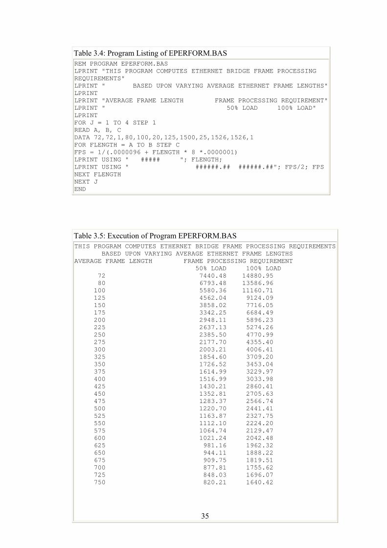
Table 3.4: Program Listing of EPERFORM.BAS REM PROGRAM EPERFORM.BAS LPRINT "THIS PROGRAM COMPUTES ETHERNET BRIDGE FRAME PROCESSING REQUIREMENTS" LPRINT " BASED UPON VARYING AVERAGE ETHERNET FRAME LENGTHS"LPRINT LPRINT "AVERAGE FRAME LENGTH FRAME PROCESSING REQUIREMENT"LPRINT " 50% LOAD 100% LOAD" LPRINT FOR J = 1 TO 4 STEP 1 READ A, B, C DATA 72,72,1,80,100,20,125,1500,25,1526,1526,1 FOR FLENGTH = A TO B STEP C FPS = 1/(.0000096 + FLENGTH * 8 *.0000001) LPRINT USING " ##### "; FLENGTH; LPRINT USING " ######.## ######.##"; FPS/2; FPS NEXT FLENGTH NEXT J END
Table 3.5: Execution of Program EPERFORM.BAS THIS PROGRAM COMPUTES ETHERNET BRIDGE FRAME PROCESSING REQUIREMENTS BASED UPON VARYING AVERAGE ETHERNET FRAME LENGTHS AVERAGE FRAME LENGTH FRAME PROCESSING REQUIREMENT 50% LOAD 100% LOAD 72 7440.48 14880.95 80 6793.48 13586.96 100 5580.36 11160.71 125 4562.04 9124.09 150 3858.02 7716.05 175 3342.25 6684.49 200 2948.11 5896.23 225 2637.13 5274.26 250 2385.50 4770.99 275 2177.70 4355.40 300 2003.21 4006.41 325 1854.60 3709.20 350 1726.52 3453.04 375 1614.99 3229.97 400 1516.99 3033.98 425 1430.21 2860.41 450 1352.81 2705.63 475 1283.37 2566.74 500 1220.70 2441.41 525 1163.87 2327.75 550 1112.10 2224.20 575 1064.74 2129.47 600 1021.24 2042.48 625 981.16 1962.32 650 944.11 1888.22 675 909.75 1819.51 700 877.81 1755.62 725 848.03 1696.07 750 820.21 1640.42
35
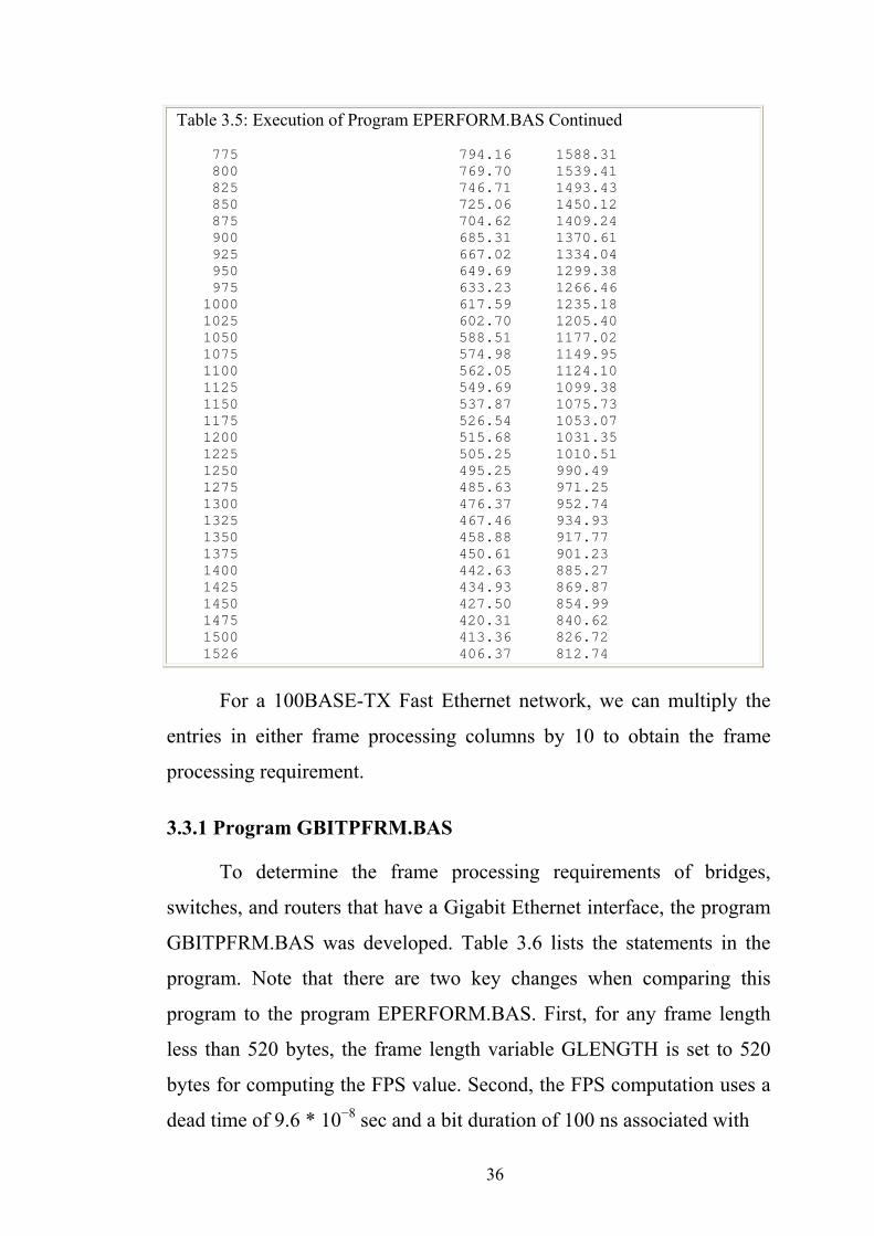
Table 3.5: Execution of Program EPERFORM.BAS Continued 775 794.16 1588.31 800 769.70 1539.41 825 746.71 1493.43 850 725.06 1450.12 875 704.62 1409.24 900 685.31 1370.61 925 667.02 1334.04 950 649.69 1299.38 975 633.23 1266.46 1000 617.59 1235.18 1025 602.70 1205.40 1050 588.51 1177.02 1075 574.98 1149.95 1100 562.05 1124.10 1125 549.69 1099.38 1150 537.87 1075.73 1175 526.54 1053.07 1200 515.68 1031.35 1225 505.25 1010.51 1250 495.25 990.49 1275 485.63 971.25 1300 476.37 952.74 1325 467.46 934.93 1350 458.88 917.77 1375 450.61 901.23 1400 442.63 885.27 1425 434.93 869.87 1450 427.50 854.99 1475 420.31 840.62 1500 413.36 826.72 1526 406.37 812.74
For a 100BASE-TX Fast Ethernet network, we can multiply the
entries in either frame processing columns by 10 to obtain the frame
processing requirement.
3.3.1 Program GBITPFRM.BAS
To determine the frame processing requirements of bridges,
switches, and routers that have a Gigabit Ethernet interface, the program
GBITPFRM.BAS was developed. Table 3.6 lists the statements in the
program. Note that there are two key changes when comparing this
program to the program EPERFORM.BAS. First, for any frame length
less than 520 bytes, the frame length variable GLENGTH is set to 520
bytes for computing the FPS value. Second, the FPS computation uses a
dead time of 9.6 * 10−8 sec and a bit duration of 100 ns associated with
36
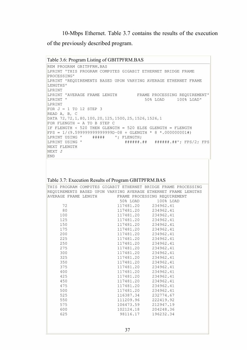
10-Mbps Ethernet. Table 3.7 contains the results of the execution
of the previously described program.
Table 3.6: Program Listing of GBITPFRM.BAS REM PROGRAM GBITPFRM.BAS LPRINT "THIS PROGRAM COMPUTES GIGABIT ETHERNET BRIDGE FRAME PROCESSING" LPRINT "REQUIREMENTS BASED UPON VARYING AVERAGE ETHERNET FRAME LENGTHS" LPRINT LPRINT "AVERAGE FRAME LENGTH FRAME PROCESSING REQUIREMENT"LPRINT " 50% LOAD 100% LOAD" LPRINT FOR J = 1 TO 12 STEP 3 READ A, B, C DATA 72,72,1,80,100,20,125,1500,25,1526,1526,1 FOR FLENGTH = A TO B STEP C IF FLENGTH < 520 THEN GLENGTH = 520 ELSE GLENGTH = FLENGTH FPS = 1/(9.599999999999999D-08 + GLENGTH * 8 *.000000001#) LPRINT USING " ##### "; FLENGTH; LPRINT USING " ######.## ######.##"; FPS/2; FPSNEXT FLENGTH NEXT J END
Table 3.7: Execution Results of Program GBITPFRM.BAS THIS PROGRAM COMPUTES GIGABIT ETHERNET BRIDGE FRAME PROCESSING REQUIREMENTS BASED UPON VARYING AVERAGE ETHERNET FRAME LENGTHS AVERAGE FRAME LENGTH FRAME PROCESSING REQUIREMENT 50% LOAD 100% LOAD 72 117481.20 234962.41 80 117481.20 234962.41 100 117481.20 234962.41 125 117481.20 234962.41 150 117481.20 234962.41 175 117481.20 234962.41 200 117481.20 234962.41 225 117481.20 234962.41 250 117481.20 234962.41 275 117481.20 234962.41 300 117481.20 234962.41 325 117481.20 234962.41 350 117481.20 234962.41 375 117481.20 234962.41 400 117481.20 234962.41 425 117481.20 234962.41 450 117481.20 234962.41 475 117481.20 234962.41 500 117481.20 234962.41 525 116387.34 232774.67 550 111209.96 222419.92 575 106473.59 212947.19 600 102124.18 204248.36 625 98116.17 196232.34
37
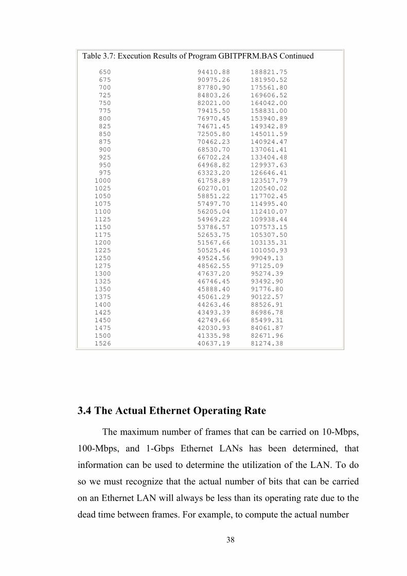
Table 3.7: Execution Results of Program GBITPFRM.BAS Continued 650 94410.88 188821.75 675 90975.26 181950.52 700 87780.90 175561.80 725 84803.26 169606.52 750 82021.00 164042.00 775 79415.50 158831.00 800 76970.45 153940.89 825 74671.45 149342.89 850 72505.80 145011.59 875 70462.23 140924.47 900 68530.70 137061.41 925 66702.24 133404.48 950 64968.82 129937.63 975 63323.20 126646.41 1000 61758.89 123517.79 1025 60270.01 120540.02 1050 58851.22 117702.45 1075 57497.70 114995.40 1100 56205.04 112410.07 1125 54969.22 109938.44 1150 53786.57 107573.15 1175 52653.75 105307.50 1200 51567.66 103135.31 1225 50525.46 101050.93 1250 49524.56 99049.13 1275 48562.55 97125.09 1300 47637.20 95274.39 1325 46746.45 93492.90 1350 45888.40 91776.80 1375 45061.29 90122.57 1400 44263.46 88526.91 1425 43493.39 86986.78 1450 42749.66 85499.31 1475 42030.93 84061.87 1500 41335.98 82671.96 1526 40637.19 81274.38
3.4 The Actual Ethernet Operating Rate
The maximum number of frames that can be carried on 10-Mbps,
100-Mbps, and 1-Gbps Ethernet LANs has been determined, that
information can be used to determine the utilization of the LAN. To do
so we must recognize that the actual number of bits that can be carried
on an Ethernet LAN will always be less than its operating rate due to the
dead time between frames. For example, to compute the actual number
38
of bits transmitted in one second using the maximum-length frame, you
must subtract the number of bits that cannot be transmitted during the
812 slots of dead time (9.6 µs for a 10-Mbps Ethernet) from the LAN
operating rate. Then, when 1526-byte frames are transmitted, the actual
maximum Ethernet network data transfer operating rate becomes:
10Mbps-9.6 µs/100ns *812=9,922,048 bps
Thus, for 100% utilization of a 10-Mbps Ethernet when a
maximum frame size of 1526 bytes is used, 9.922 Mbps must be
transmitted in one second.
For a Fast Ethernet LAN, idle characters are transmitted between
frames, which in effect results in a dead time between frames. That dead
time is one tenth that of a 10-Mbps Ethernet, or 0.96 µs, while the bit
duration is reduced to 10 ns. Thus, the actual maximum 100-Mbps Fast
Ethernet data transfer operating rate when 1526-byte frames are
transmitted becomes:
100Mbps-0.96 µs/10ns *8127=99,220,480 bps
We can perform a similar computation for Gigabit Ethernet,
adjusting the dead time between frames, its bit duration, and the number
of frames transportable per second as follows for maximum length
frames:
1000Mbps-0.096 µs/1ns *81275=992,197,600 bps
So due to the dead time between the frames only 99% of the
transmission rate could be used.
39
3.5 Network Utilization:
To illustrate the computations required to determine the level of
Ethernet network utilization, let us assume that the monitoring of an
Ethernet LAN indicates that during 10 minutes of monitoring, a total of
280,000 frames with an average data field length of 100 bytes were
counted. The average frame length, including 100 data bytes, would be
126 bytes due to the 26 overhead bytes required to transport each frame.
Then the average number of frames per second would be computed as
follows:
280000 frames/10 minutes=466.67 frames per second
The number of bits flowing on the network is computed by
multiplying the frame size by 8 bits/byte and then multiplying the result
by the frame size. Thus, 126 bytes/frame * 8 bits/byte * 466.67
frames/second is 470,403 bits. Then, the utilization in percent would be
470,403/9,922,048 * 100, or 4.74%.
Based on readily available performance statistics, a 100-node
Ethernet can normally be expected to have an average utilization under 2
percent, with worst second, minute, and hour percentages of 40, 15 to 20,
and 3 to 5, respectively. Similar utilization levels may not be applicable
to 100-Mbps Fast Ethernet networks because such networks operate at
ten times the rate of 10BASE-T LANs. This means that they can support
a significant increase in traffic prior to reaching a higher level of
utilization.
These preceding performance statistics represent the activity on a
typical Ethernet network in that, at any particular time, many network
users are performing local processing, such as composing a
memorandum or an electronic message. Other network users may be
40
reading a manual, talking on the telephone, or performing an activity
completely unrelated to network usage. Thus, only a few people are
actually transmitting or receiving information using the network.
Concerning those people, one network user may be transmitting a short
electronic mail message of a few hundred characters while another
network user might be downloading a file from the server or accessing a
server facility. Thus, a typical 2-percent level of network utilization on a
10-Mbps Ethernet network equates to a data transfer of 9,922,048 * 0.02,
or approximately 198 Kbps. At this data transfer rate, many people can
be sending electronic messages, interacting with the file server, and
performing file transfer operations.
On a Fast Ethernet network, a 2-percent level of network
utilization equates to a data transfer rate ten times that of a 10-Mbps
Ethernet network, or approximately 1.98 Mbps. To put this number in
perspective, let us assume that the typical length of an electronic mail
message is 1000 characters, or 8000 bits. This means that at a 2-percent
level of network utilization, a 100-Mbps Fast Ethernet network could
support the transfer of almost 250 1000-character electronic mail
messages per second!
When a number of network users initiate file transfers, you can
expect a short peak level of utilization to approach or surpass 40 percent
on a 10-Mbps Ethernet network. Because a 640-Kbyte file transfer will
require less than 0.07 seconds at 10 Mbps, many file transfers will
rapidly be completed, which eliminates the potential for one file transfer
overlapping another file transfer operation if two people initiate a file
transfer just a second or two apart from one another. This explains why
the worst minute utilization of a 10-Mbps Ethernet network is typically
reduced to a range between 15 and 20 percent in comparison to a worst
41
second utilization of 40 percent. Because our previous computation is
much better than the typical worst minute utilization, it would appear
that the monitored LAN is not overloaded. However, an extension of
monitoring of several hours of activity during peak periods should be
considered to ensure that utilization peaks were not inadvertently missed.
3.6 Information Transfer Rate
Although knowledge concerning the average frame length and
frame rate is important, by themselves they do not provide definitive
information concerning the rate at which information can be transferred
on a network. This is because a portion of an Ethernet frame represents
overhead and does not carry actual data. Thus, to obtain a more realistic
indication of the ability of an Ethernet network to transfer information,
you must compute the information transfer rate in bits per second (bps).
This calculation is performed by first subtracting 26 bytes from the
frame length for frames with a data field of 46 or more bytes, as there are
26 overhead bytes in each frame. Next, you would multiply the frame
rate by the adjusted frame length and then multiply the result by 8 to
obtain the information transfer rate in bits per second.
Table 3.8 lists the statements contained in a program named
EITR.BAS. This program was developed to compute the information
transfer rate in bps based on 16 average frame lengths and their
corresponding frame transfer rates.
The results of the execution of EITR.BAS are listed in Table 3.9.
To obtain the frames per second and information transfer rate for Fast
Ethernet, you can multiply the entries in the second and third columns of
Table 3.9 by 10.
42
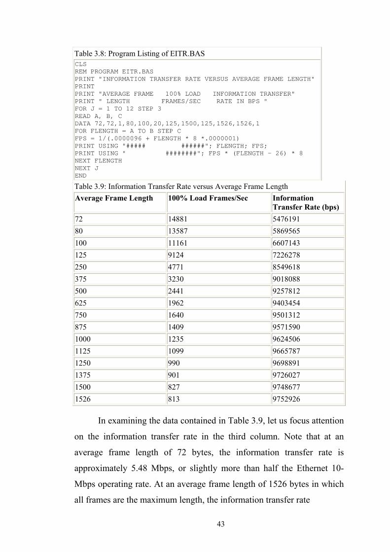
Table 3.8: Program Listing of EITR.BAS CLS REM PROGRAM EITR.BAS PRINT "INFORMATION TRANSFER RATE VERSUS AVERAGE FRAME LENGTH" PRINT PRINT "AVERAGE FRAME 100% LOAD INFORMATION TRANSFER" PRINT " LENGTH FRAMES/SEC RATE IN BPS " FOR J = 1 TO 12 STEP 3 READ A, B, C DATA 72,72,1,80,100,20,125,1500,125,1526,1526,1 FOR FLENGTH = A TO B STEP C FPS = 1/(.0000096 + FLENGTH * 8 *.0000001) PRINT USING "##### ######"; FLENGTH; FPS; PRINT USING " ########"; FPS * (FLENGTH - 26) * 8 NEXT FLENGTH NEXT J END
Table 3.9: Information Transfer Rate versus Average Frame Length Average Frame Length 100% Load Frames/Sec Information
Transfer Rate (bps) 72 14881 5476191 80 13587 5869565 100 11161 6607143 125 9124 7226278 250 4771 8549618 375 3230 9018088 500 2441 9257812 625 1962 9403454 750 1640 9501312 875 1409 9571590 1000 1235 9624506 1125 1099 9665787 1250 990 9698891 1375 901 9726027 1500 827 9748677 1526 813 9752926
In examining the data contained in Table 3.9, let us focus attention
on the information transfer rate in the third column. Note that at an
average frame length of 72 bytes, the information transfer rate is
approximately 5.48 Mbps, or slightly more than half the Ethernet 10-
Mbps operating rate. At an average frame length of 1526 bytes in which
all frames are the maximum length, the information transfer rate
43
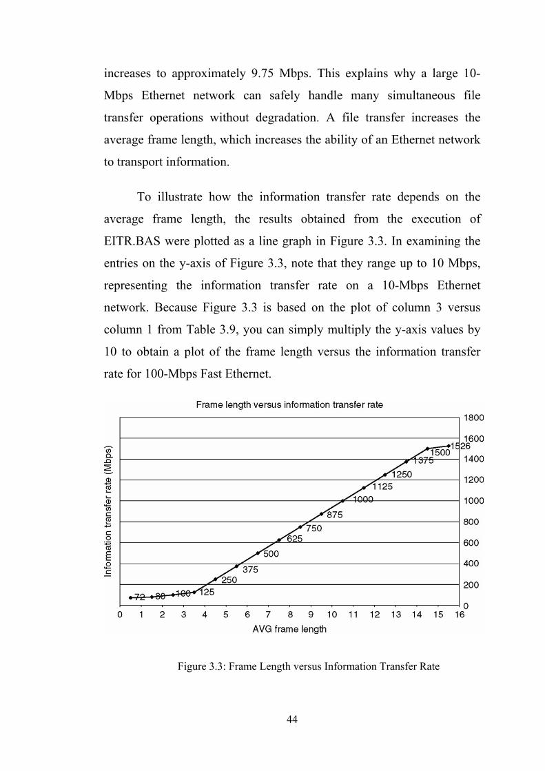
increases to approximately 9.75 Mbps. This explains why a large 10-
Mbps Ethernet network can safely handle many simultaneous file
transfer operations without degradation. A file transfer increases the
average frame length, which increases the ability of an Ethernet network
to transport information.
To illustrate how the information transfer rate depends on the
average frame length, the results obtained from the execution of
EITR.BAS were plotted as a line graph in Figure 3.3. In examining the
entries on the y-axis of Figure 3.3, note that they range up to 10 Mbps,
representing the information transfer rate on a 10-Mbps Ethernet
network. Because Figure 3.3 is based on the plot of column 3 versus
column 1 from Table 3.9, you can simply multiply the y-axis values by
10 to obtain a plot of the frame length versus the information transfer
rate for 100-Mbps Fast Ethernet.
Figure 3.3: Frame Length versus Information Transfer Rate
44
3.6.1 Gigabit Ethernet Considerations
As previously noted, Gigabit frames less than 512 bytes in length,
not including the preamble and start of frame delimiter fields, are
extended to a length of 512 bytes through carrier extension technology.
Thus, the actual information transfer capacity of a Gigabit frame depends
on its length.
Table 3.10 contains the program listing of GITR.BAS, which was
developed to compute the information transfer rate of Gigabit Ethernet
based on a range of frame lengths. Note that when the frame length is
less than 500, that value plus 8 is subtracted from 512 to determine the
number of carrier extensions. Because we are working with frames that
include the preamble and start of frame delimiter fields, an additional 8
bytes is subtracted to determine the number of carrier extensions. Next,
the LPRINT statement subtracts the number of carrier extensions plus 26
overhead Ethernet bytes from the fixed Gigabit frame length of 520
bytes for all frames less than or equal to 520 and multiplies that amount
by 8 to compute the number of information transporting bits in a frame.
Multiplying that number by the variable FPS results in the information
transfer rate for all frames up to 520 bytes in length. When frames
exceed 520 bytes in length, the second series of LPRINT statements is
invoked. This results in the frame length being decremented by the 26
overhead bytes in order to compute the information transfer rate. Table
3.11 illustrates the results obtained from the execution of the program
GITR.BAS.
45
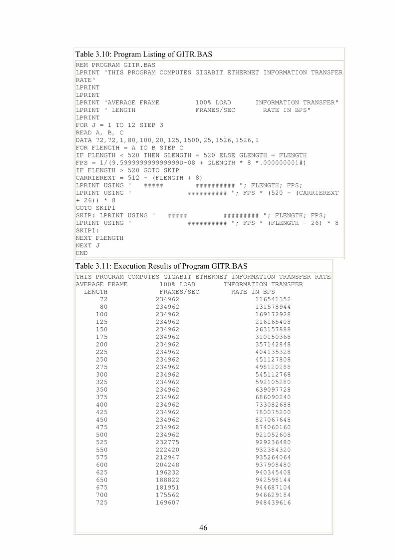
Table 3.10: Program Listing of GITR.BAS REM PROGRAM GITR.BAS LPRINT "THIS PROGRAM COMPUTES GIGABIT ETHERNET INFORMATION TRANSFERRATE" LPRINT LPRINT LPRINT "AVERAGE FRAME 100% LOAD INFORMATION TRANSFER" LPRINT " LENGTH FRAMES/SEC RATE IN BPS" LPRINT FOR J = 1 TO 12 STEP 3 READ A, B, C DATA 72,72,1,80,100,20,125,1500,25,1526,1526,1 FOR FLENGTH = A TO B STEP C IF FLENGTH < 520 THEN GLENGTH = 520 ELSE GLENGTH = FLENGTH FPS = 1/(9.599999999999999D-08 + GLENGTH * 8 *.000000001#) IF FLENGTH > 520 GOTO SKIP CARRIEREXT = 512 - (FLENGTH + 8) LPRINT USING " ##### ########## "; FLENGTH; FPS; LPRINT USING " ########## "; FPS * (520 - (CARRIEREXT + 26)) * 8 GOTO SKIP1 SKIP: LPRINT USING " ##### ######### "; FLENGTH; FPS; LPRINT USING " ########## "; FPS * (FLENGTH - 26) * 8 SKIP1: NEXT FLENGTH NEXT J END
Table 3.11: Execution Results of Program GITR.BAS THIS PROGRAM COMPUTES GIGABIT ETHERNET INFORMATION TRANSFER RATEAVERAGE FRAME 100% LOAD INFORMATION TRANSFER LENGTH FRAMES/SEC RATE IN BPS 72 234962 116541352 80 234962 131578944 100 234962 169172928 125 234962 216165408 150 234962 263157888 175 234962 310150368 200 234962 357142848 225 234962 404135328 250 234962 451127808 275 234962 498120288 300 234962 545112768 325 234962 592105280 350 234962 639097728 375 234962 686090240 400 234962 733082688 425 234962 780075200 450 234962 827067648 475 234962 874060160 500 234962 921052608 525 232775 929236480 550 222420 932384320 575 212947 935264064 600 204248 937908480 625 196232 940345408 650 188822 942598144 675 181951 944687104 700 175562 946629184 725 169607 948439616
46
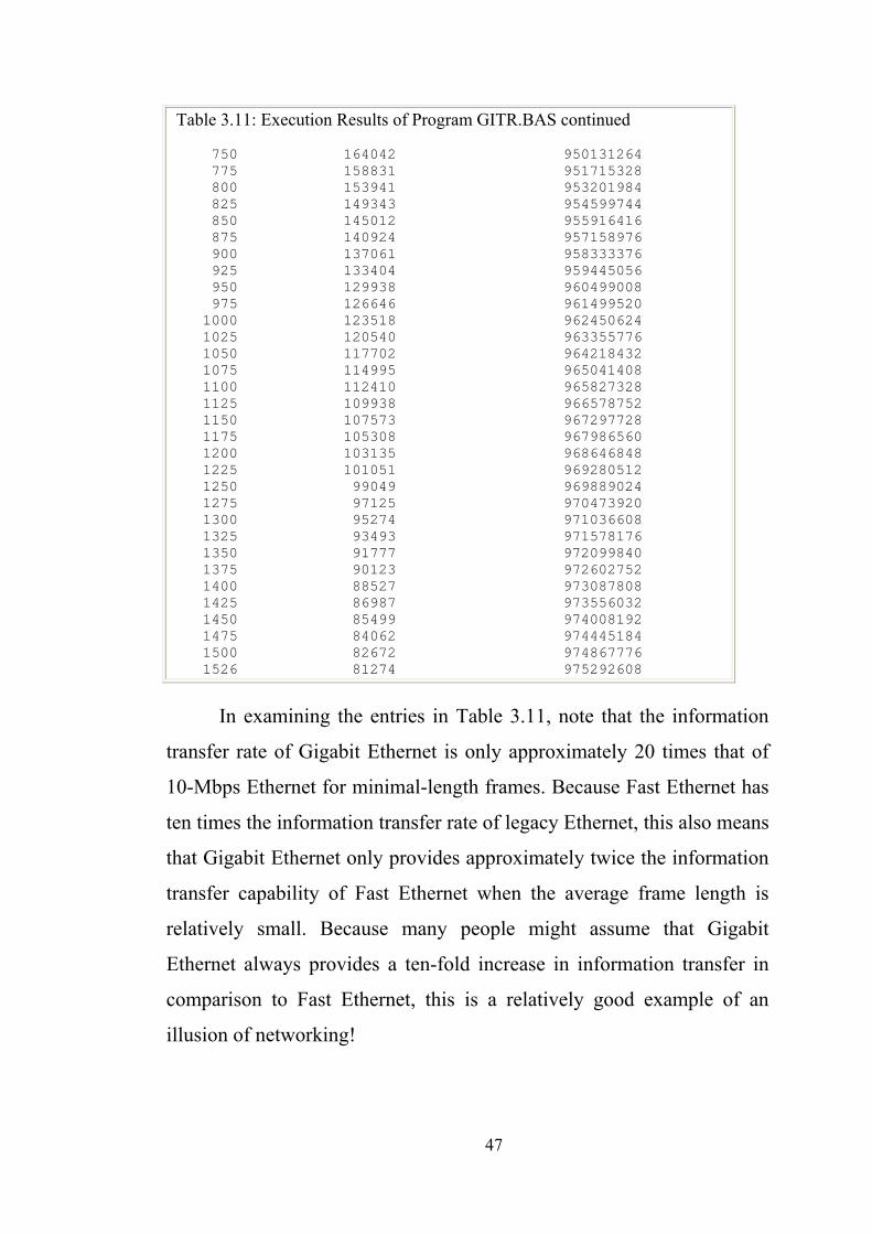
Table 3.11: Execution Results of Program GITR.BAS continued 750 164042 950131264 775 158831 951715328 800 153941 953201984 825 149343 954599744 850 145012 955916416 875 140924 957158976 900 137061 958333376 925 133404 959445056 950 129938 960499008 975 126646 961499520 1000 123518 962450624 1025 120540 963355776 1050 117702 964218432 1075 114995 965041408 1100 112410 965827328 1125 109938 966578752 1150 107573 967297728 1175 105308 967986560 1200 103135 968646848 1225 101051 969280512 1250 99049 969889024 1275 97125 970473920 1300 95274 971036608 1325 93493 971578176 1350 91777 972099840 1375 90123 972602752 1400 88527 973087808 1425 86987 973556032 1450 85499 974008192 1475 84062 974445184 1500 82672 974867776 1526 81274 975292608
In examining the entries in Table 3.11, note that the information
transfer rate of Gigabit Ethernet is only approximately 20 times that of
10-Mbps Ethernet for minimal-length frames. Because Fast Ethernet has
ten times the information transfer rate of legacy Ethernet, this also means
that Gigabit Ethernet only provides approximately twice the information
transfer capability of Fast Ethernet when the average frame length is
relatively small. Because many people might assume that Gigabit
Ethernet always provides a ten-fold increase in information transfer in
comparison to Fast Ethernet, this is a relatively good example of an
illusion of networking!
47
In our examination of the overhead associated with the
composition of Ethernet frames, we noted that relatively short frames
have a relatively large overhead, owing to the necessity to use pad
characters to fill a data field to a minimum of 46 characters. At that time,
we noted that by composing a client screen to accept several items of
information rather than perform separate queries, we could enhance the
efficiency of Ethernet frames, as they would transport larger data fields.
At that time we did not notice an optimum data field size other than the
fact that a minimum data field of 1500 characters is the most efficient.
48
Chapter Four
Factors Affecting Token Ring Network Performance
Chapter Four
Factors Affecting Token Ring Network Performance
For the Ethernet network performance we developed a
mathematical model to determine the frame rate based on different frame
lengths. The results of that model were then used to determine the
information transfer capability of a 10-Mbps Ethernet network based on
different frame sizes. As might be intuitively expect, the use of larger
frames provided a higher information transfer capability because each
Ethernet frame is separated from preceding and succeeding frames by a
uniform time gap. Thus, longer frames were expected to be more
efficient and this was determined to be true.
In this chapter, our attention will turn to Token Ring network
performance in a similar manner to our method of examining Ethernet
performance. That is, we will first develop a model that is representative
of the flow of data on a Token Ring network. Then we will exercise the
model both manually as well as through the use of a BASIC language
program to determine the frame rate as a function of the number of
stations on the network and the ring length as well as several other
variables. In doing so, we will note that the performance models for
CSMA/CD and Token Ring networks considerably differ due to the
basic differences between each network access protocol.
In a CSMA/CD network, the transmission of a frame is read by all
stations without one station's reading activity delaying another station's
reading activity. In a Token Ring network, the opposite is true, because
station n must process a token or frame prior to passing it onto station
n+1 on the network. Thus, the Token Ring model developed in this
49
chapter will considerably differ from the previously developed Ethernet
model. A second area of difference concerns the cabling structure of
Ethernet and Token Ring networks. Most Ethernet bus-based networks
use a fraction of the cabling used in the star-bus topology of a Token
Ring network. Thus, propagation delay time plays a much more
meaningful role in determining network performance and results in our
inclusion of the speed at which tokens and frames traverse the cable in
the Token Ring model we develop in this chapter.
4.1 Operation of Token-Passing Ring LANs
In a token-passing ring local area network, the shared transmission
medium is closed on itself and takes the form of a loop as shown in
Figure 4.1(a). The information flow is only in one direction. Access to
the transmission medium is regulated with the help of a token a small
packet that consists of about eight bits. The token has two possible
states: free and busy. A free token indicates that transmission medium is
available for transmission; a busy token indicates that the transmission
medium is busy.
50
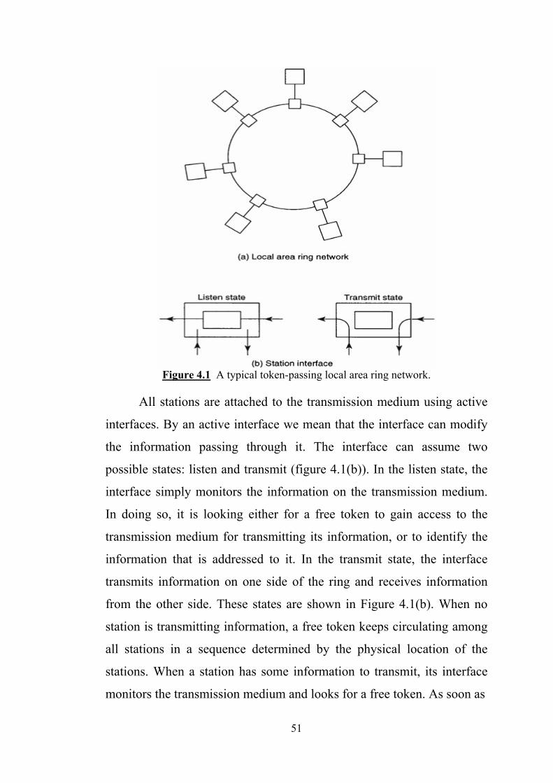
Figure 4.1 A typical token-passing local area ring network.
All stations are attached to the transmission medium using active
interfaces. By an active interface we mean that the interface can modify
the information passing through it. The interface can assume two
possible states: listen and transmit (figure 4.1(b)). In the listen state, the
interface simply monitors the information on the transmission medium.
In doing so, it is looking either for a free token to gain access to the
transmission medium for transmitting its information, or to identify the
information that is addressed to it. In the transmit state, the interface
transmits information on one side of the ring and receives information
from the other side. These states are shown in Figure 4.1(b). When no
station is transmitting information, a free token keeps circulating among
all stations in a sequence determined by the physical location of the
stations. When a station has some information to transmit, its interface
monitors the transmission medium and looks for a free token. As soon as
51
it sees a free token, it captures the token, makes it a busy token (by
changing its last bit), and immediately transmits the information. While a
station is transmitting, the ring is practically broken at the location of the
transmitting station. The station injects information onto the ring from
one side and removes information from the other. As the information
goes around the ring, other stations monitor the transmission medium
identifying the information that belongs to them. As a station finds
information addressed to it, the information is copied (not removed) by
the station. The transmitting station is responsible for removing its
information from the ring. Once a station completes its transmission, it
regenerates a free token so that other stations may have the opportunity
to transmit their information. This process continues, and every station
waits for its turn to use the transmission medium.
Once a station captures a free token to gain access to the
transmission medium, it can theoretically keep the token for an indefinite
period of time. However, this is unacceptable because all stations need a
free token to transmit their information. The token must be released
(regenerated) by a station after it has used the transmission medium for a
certain period of time (called the token-holding time).
There are three well-defined schemes, referred to as service
disciplines that can be used to limit the token-holding time in token-
passing LANs: exhaustive, gated, and limited-k. In the exhaustive
service discipline, once a station captures a free token, it is allowed to
use the transmission medium until its buffer becomes empty and the
station regenerates the free token so that the next station may capture it
to use the transmission medium. In the gated service discipline, a station
is allowed to transmit only as many packets of information as were
present in its buffer when a free token was captured and then the station
52
regenerate the token. All packets that arrive during the transmission of
packets present in the buffer must wait until the next time a free token is
captured. In limited-k service discipline, a station is allowed to transmit a
maximum of k (k = 1, 2, 3, . . .) packets when it captures a free token. A
free token is regenerated either immediately after k packets have been
transmitted or when the buffer becomes empty.
Token-holding time also depends upon when a station decides to
regenerate a free token. There are three types of operation defined in this
regard: multiple-token operation, single-token operation, and single-
packet operation. In multiple-token operation, a station regenerates a free
token immediately after it has completed the transmission of the last bit
of its information. In single-token operation, a station regenerates a free
token after it has transmitted the last bit of its information and after it has
removed the busy token from the ring. Multiple-token and single- token
operations behave in exactly the same way if the packet transmission
time is more than the ring latency (the time it takes for a bit to travel
around the ring). However, if the packet transmission time is less than
the ring latency, the performance of these two operations is quite
different. Single-packet operation is a more rigid operation in terms of its
requirements for regenerating a free token. In this operation a free token
is regenerated only after the last bit of transmitted information has been
removed from the ring. The ring must be absolutely free before a free
token can be regenerated.
4.2 Token Ring Traffic Modeling
Compared to Ethernet, the modeling of a Token Ring network can
be much more complex. This is because the frame rate depends on the
number of nodes in a network, the token holding time per node, the type
53
of wire used for cabling and ring length, and the type of adapter used as
a ring interface unit.
The number of nodes and their cabling govern both token propagation
time and holding time as a token flow around the ring. The type of
adapter used governs the maximum frame rate supported. This rate can
vary between vendors as well as within a vendor's product line.
The type of cabling and ring length governs the propagation delay
associated with the flow of tokens and frames around the ring. Although
the data rate around a ring is consistent at either 4 Mbps or 16 Mbps,
tokens and frames do not flow instantaneously around the ring and are
delayed based upon the distance they must traverse and the type of
cabling used. In addition, a slight delay is encountered at each node
because the token must be examined to determine its status.
4.3 Model Development
Let us assume there are N stations on the network. Then, on
average, a token will travel N/2 stations until it is grabbed and converted
into a frame. Similarly, a frame can be expected to travel N/2 stations
until it reaches its destination and another N/2 stations until it returns to
the origination station and is reconverted into a token.
4.4 Propagation Delay
In free space, the velocity of light is 3*108 m/s. In twisted pair
cable, the speed of electrons is approximately 62% of the velocity of
light in free space. Thus, electrons will travel at approximately
(3x108x0.62), or (186x106 m/s). Then, to traverse 1000 meter (1km) of
cable would require 1000/ (186x106), or approximately 5.38 x10⁻⁶ (5.38
µs).
54
At a Token Ring operating rate of 4 Mbps, the bit duration is
1/4,000,000, or 2.5 x 10⁻⁷ seconds. At a network operating rate of 16
Mbps, the bit duration is 1/16,000,000, or 0.625 x 10⁻⁷ seconds. Because
the time required for electrons to traverse 1000 meter of cable is 5.38 µs,
the cable propagation delay time per 1000 meter of cable can be
converted into a bit time delay to simplify computations. At a Token
Ring operating rate of 4 Mbps, the bit time delay per 1000 meter of cable
becomes 5.38 x10⁻⁶ / 2.5 x 10⁻⁷, or 21.52 bit times. When the Token Ring
network operates at 16 Mbps, the bit time delay per 1000 meter of cable
becomes 5.38 x10⁻⁶ / 0.625x10⁻⁷, or 86.08 bit times.
4.5 4-Mbps Model
For the development of a 4-Mbps Token Ring performance model,
let us start with the flow of a token as indicated by the following steps in
the model development process.
1. Given a Token Ring network with N stations, a free token travels,
on average, N/2 stations until it is grabbed and converted into a
frame.
2. Each station adds a 2.5-bit time delay to examine the token. At a
4-Mbps ring operating rate, a bit time equals 2.5 * 10−7 seconds.
Thus, each station induces a delay of 2.5 * 2.5 * 10−7, or 6.25 *
10−7 seconds.
3. The token consists of 3 bytes, or 24 bits. The time required for the
token to be placed onto the ring is:
24 x 2.5 x 10-7 sec/bit =60 x 10-7 seconds = 6 µs
55
4. The time for the token to be placed onto the ring and flow around
half the ring until it is grabbed is the sum of the times of step 2
and step 3. This time then becomes:
N/2 x 6.25 x 10-7 +60 x 10-7
5. Once a token is grabbed, it is converted into a frame. On average,
the frame will travel N/2 stations to its destination. A frame
containing 64 bytes of information consists of 85 bytes because 21
bytes of overhead, including starting and ending delimiters, source
and destination addresses, and other control information must be
included in the frame. Thus, the time required to place the frame
on the ring becomes:
85 bytes x 8 bit/byte x 2.5 x 10⁻⁷ seconds/bit =1.7 x 10⁻⁴
6. The frame must traverse N/2 stations, on average, to reach its
destination. Thus, the time required for the frame to be placed
onto the ring and traverse half the ring becomes:
1.7 x 10⁻⁴ +N/2 x 6.25 x 10-7 seconds
7. The total token and frame time from numbers 4 and 6 above is:
N/2 x 6.25 x 10-7 +60 x 10-7 + N/2 x 6.25 x 10-7 +1.7 x 10-4
= N x 6.25 x 10⁻⁷ +60 x 10-7 + 1.7 x 10⁻⁴ seconds
8. Once the frame reaches its destination, it must traverse another
N/2 stations, on average, to return to its originating station, which
then removes it from the network. Then, the origination station
generates a new token onto the network and the previously
56
described process is repeated. The time for the frame to again traverse
half the network becomes:
N/2 x 6.25 x 10-7 seconds
This time must be added to the time in step 7. Doing so, we
obtain:
N x 9.375 x 10⁻⁷ +60 x 10-7 + 1.7 x 10⁻⁴ seconds
9. To consider the effect of propagation delay time as tokens and
frames flow in the cable, we must consider the sum of the ring
length and twice the sum of all lobe distances. Here, we must
double the lobe distances because the token will flow to and from
each workstation on the lobe. If we let C equal the number of
thousands of meter of cable, we obtain the time in seconds to
traverse the ring as:
N x 9.375 x 10⁻⁷ +60 x 10-7 + 1.7 x 10⁻⁴ +5.38 x 10⁻⁶ x C
which equals:
N x 9.375 x 10⁻⁷ +1.76 x 10⁻⁴ +5.38 x 10⁻⁶ x C
where:
N = number of stations
C = thousands of meters of cable
4.6 Exercising the Model
To illustrate the use of the previously developed Token Ring
performance model, let us assume a Token Ring network of 50 stations
57
has 8000 meter of cable. Then, the time for a token and frame to
circulate the ring becomes:
50 x 9.375 x 10-7 +1.76 x 10⁻⁴ +5.38 x 10-6 x 8
=468.75 x 10⁻⁷ +1.76 x 10⁻⁴ +43.04 x 10-6
=0.46875 x 10⁻⁴ +1.76 x 10⁻⁴ +0.4304 x 10-4
=2.6592 x 10⁻⁴ seconds=0.2659 ms
Then, in 1 second there will be, on average, 1/(0.2659 * 10−3 ), or 3760
64-byte information frames that can flow on a Token Ring network
containing 50 stations and a total of 8000 meter of cable.
4.7 Network Modification
To determine the effect of cabling length and the number of the
network stations on the frame rate, let us now consider what happens
when we reduce the size of the network. Suppose the number of
workstations is reduced to 25 and the total cable distance reduced to
4000 meter. Then, with N = 25 and C = 4, the time for a token and frame
to flow around the ring becomes:
25 x 9.375 x 10-7 +1.76 x 10⁻⁴ +5.38 x 10-6 x 4
=0.234375 x 10⁻⁴ +1.76 x 10⁻⁴ +0.2152 x 10-4
=2.21 x 10⁻⁴ seconds=0.221 ms
Thus, in 1 second there will be, on average, 1/ (0.221 x 10⁻³), or
4524 of 64-byte information frames. As we would intuitively expect, as
the number of stations and cable distance decrease, the transmission
capacity of the ring increases.
58
4.8 Varying the Frame Size
Suppose we transmit 4000-byte information frames. Here, a total
of 4021 bytes is required. Thus, the time required for the frame to be
placed on the ring becomes:
4021x8x2.5x10-7, or 8.042 ms
Then, the total token and frame time becomes:
Nx9.375x10-7+60x10-7+8.042x10⁻³+5.38 x 10⁻⁶xC
Again, let us assume the number of stations, N, is 50, while the cabling
distance is 8000 meter. Thus, we obtain the token and frame revolution
time as follows:
50x9.375x10-7+60x10-7+8.042x10⁻³+5.38 x 10-6 x8 =8.138 ms
Thus, in 1 second there will be 1/(8.138 x 10−3) or 122 frames. Because
each frame contains 4000 bytes of information, the effective operating
rate becomes 122 x 4000 x 8, or 3.904 Mbps for a 50-station Token Ring
network with 8000 meter of cable using 4000 character information
frames. In comparison, a similar Token Ring network using 64-byte
information frames would have a frame rate of 4760 frames per second.
However, this rate would be equivalent to an information transfer rate of
3760 x 64 x 8, or 1.925 Mbps. Thus, larger frame sizes provide a more
efficient data transportation capability.
This means, the frame length, cabling distance, and number of network
stations govern the maximum frame rate that can flow on a Token Ring
network. This tells us that when a network becomes saturated due to
heavy usage, you should consider breaking larger networks into two or
59
more subnets interconnected by bridges to improve Token Ring network
performance.
4.9 General Model Development
We have developed and exercised a mathematical model to
determine the frame rate on a 4-Mbps Token Ring network; we will use
our prior effort to develop a general model for 4- and 16-Mbps networks.
In doing so, let us use BASIC language variables so that we can exercise
our model through its incorporation into a BASIC language program.
To denote the difference between 4- and 16-Mbps networks, let us
use the array variable BITTIME(1). Then, we can assign the value
1/4,000,000 to BITTIME(1) to represent the bit time duration on a 4-
Mbps Token Ring network and the value 1/16,000,000 to BITTIME(2)
to represent the bit time duration on a 16-Mbps network.
Using the variable S.DELAY to represent the station delay, we obtain:
S.DELAY = 2.5 * BITTIME(1)
Using the variable T.PLACEMENT to represent the token placement
time, we obtain:
T.PLACEMENT = 24 * BITTIME(1)
Then, using the variable H.TRINGFLOW to represent the time for a
token to be placed on the network and traverse half the ring (step 4 in our
earlier model), we obtain:
H.TRINGLOW = (N/2) * S.DELAY + T.PLACEMENT
Once a token is grabbed, it is converted into a frame. Because the time
required to place the frame onto the ring depends on the length of the
60
frame, let us use the array variable FRAMELENGTH(F) to denote
different frame lengths, and add 21 bytes to represent the overhead per
frame. Then, if we use the variable FRAMETIME to denote the time
required to place a frame on the ring, we obtain:
FRAMETIME = (FRAMELENGTH(F) + 21) * 8 * BITTIME(1)
If we denote the variable H.FRAMEFLOW to represent the time
required for the frame to be placed on the ring and flow N/2 stations
down the ring, we obtain:
H.FRAMEFLOW = (N/2) * S.DELAY + FRAMETIME
If we use the variable C to denote the cable length (ring plus twice each
lobe distance) in 1000-meter increments and the variable C.PROPTIME
to denote the propagation delay time, we obtain:
C.PROPTIME = C * 5.38 * 10-6
Then, to compute the frame rate using the variable FPS, we obtain:
FPS = 1/(TOTAL.TIME + C.PROPTIME)
4.10 Program TPERFORM.BAS
This program can be used to generate a series of tables that
indicates the frame rate based upon the network operating rate, number
of stations on the network, average frame length, and network cable
length in 1000-meter increments. As previously noted, the frame length
is specified in terms of the information field to which 21 bytes
representing frame overhead are added.
61
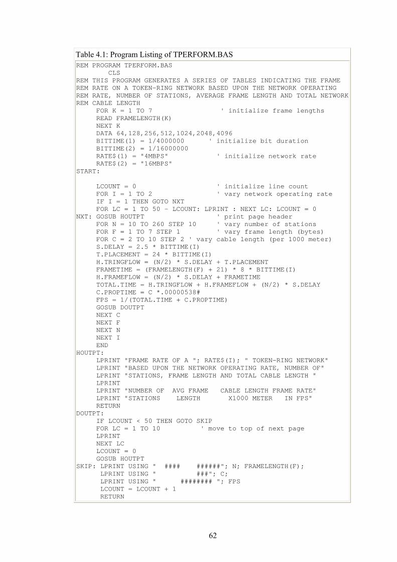
Table 4.1: Program Listing of TPERFORM.BAS REM PROGRAM TPERFORM.BAS CLS REM THIS PROGRAM GENERATES A SERIES OF TABLES INDICATING THE FRAME REM RATE ON A TOKEN-RING NETWORK BASED UPON THE NETWORK OPERATING REM RATE, NUMBER OF STATIONS, AVERAGE FRAME LENGTH AND TOTAL NETWORKREM CABLE LENGTH FOR K = 1 TO 7 ' initialize frame lengths READ FRAMELENGTH(K) NEXT K DATA 64,128,256,512,1024,2048,4096 BITTIME(1) = 1/4000000 ' initialize bit duration BITTIME(2) = 1/16000000 RATE$(1) = "4MBPS" ' initialize network rate RATE$(2) = "16MBPS" START: LCOUNT = 0 ' initialize line count FOR I = 1 TO 2 ' vary network operating rate IF I = 1 THEN GOTO NXT FOR LC = 1 TO 50 - LCOUNT: LPRINT : NEXT LC: LCOUNT = 0 NXT: GOSUB HOUTPT ' print page header FOR N = 10 TO 260 STEP 10 ' vary number of stations FOR F = 1 TO 7 STEP 1 ' vary frame length (bytes) FOR C = 2 TO 10 STEP 2 ' vary cable length (per 1000 meter) S.DELAY = 2.5 * BITTIME(I) T.PLACEMENT = 24 * BITTIME(I) H.TRINGFLOW = (N/2) * S.DELAY + T.PLACEMENT FRAMETIME = (FRAMELENGTH(F) + 21) * 8 * BITTIME(I) H.FRAMEFLOW = (N/2) * S.DELAY + FRAMETIME TOTAL.TIME = H.TRINGFLOW + H.FRAMEFLOW + (N/2) * S.DELAY C.PROPTIME = C *.00000538# FPS = 1/(TOTAL.TIME + C.PROPTIME) GOSUB DOUTPT NEXT C NEXT F NEXT N NEXT I END HOUTPT: LPRINT "FRAME RATE OF A "; RATE$(I); " TOKEN-RING NETWORK" LPRINT "BASED UPON THE NETWORK OPERATING RATE, NUMBER OF" LPRINT "STATIONS, FRAME LENGTH AND TOTAL CABLE LENGTH " LPRINT LPRINT "NUMBER OF AVG FRAME CABLE LENGTH FRAME RATE" LPRINT "STATIONS LENGTH X1000 METER IN FPS" RETURN DOUTPT: IF LCOUNT < 50 THEN GOTO SKIP FOR LC = 1 TO 10 ' move to top of next page LPRINT NEXT LC LCOUNT = 0 GOSUB HOUTPT SKIP: LPRINT USING " #### ######"; N; FRAMELENGTH(F); LPRINT USING " ###"; C; LPRINT USING " ######## "; FPS LCOUNT = LCOUNT + 1 RETURN
62
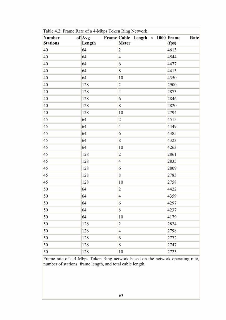
Table 4.2: Frame Rate of a 4-Mbps Token Ring Network Number of Stations
Avg Frame Length
Cable Length × 1000 Meter
Frame Rate (fps)
40 64 2 4613 40 64 4 4544 40 64 6 4477 40 64 8 4413 40 64 10 4350 40 128 2 2900 40 128 4 2873 40 128 6 2846 40 128 8 2820 40 128 10 2794 45 64 2 4515 45 64 4 4449 45 64 6 4385 45 64 8 4323 45 64 10 4263 45 128 2 2861 45 128 4 2835 45 128 6 2809 45 128 8 2783 45 128 10 2758 50 64 2 4422 50 64 4 4359 50 64 6 4297 50 64 8 4237 50 64 10 4179 50 128 2 2824 50 128 4 2798 50 128 6 2772 50 128 8 2747 50 128 10 2723 Frame rate of a 4-Mbps Token Ring network based on the network operating rate, number of stations, frame length, and total cable length.
63
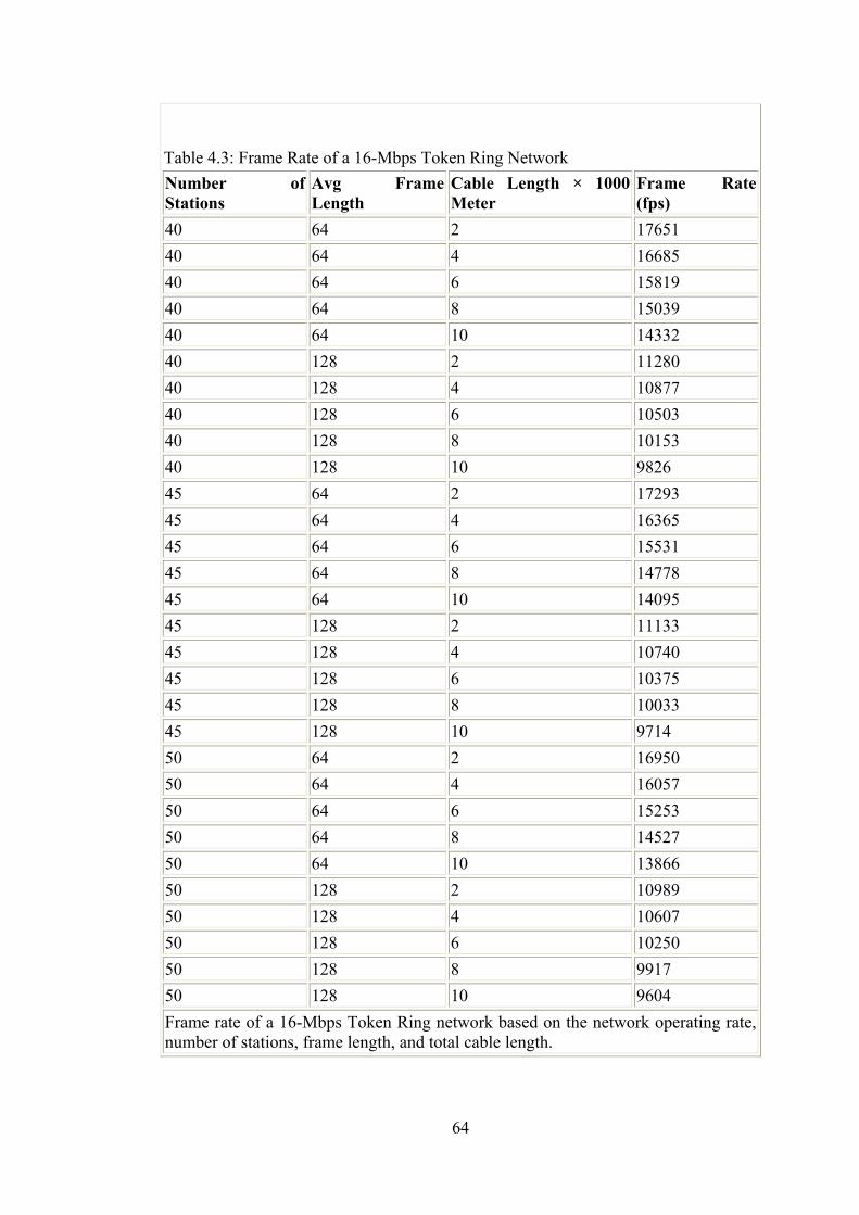
Table 4.3: Frame Rate of a 16-Mbps Token Ring Network Number of Stations
Avg Frame Length
Cable Length × 1000 Meter
Frame Rate (fps)
40 64 2 17651 40 64 4 16685 40 64 6 15819 40 64 8 15039 40 64 10 14332 40 128 2 11280 40 128 4 10877 40 128 6 10503 40 128 8 10153 40 128 10 9826 45 64 2 17293 45 64 4 16365 45 64 6 15531 45 64 8 14778 45 64 10 14095 45 128 2 11133 45 128 4 10740 45 128 6 10375 45 128 8 10033 45 128 10 9714 50 64 2 16950 50 64 4 16057 50 64 6 15253 50 64 8 14527 50 64 10 13866 50 128 2 10989 50 128 4 10607 50 128 6 10250 50 128 8 9917 50 128 10 9604 Frame rate of a 16-Mbps Token Ring network based on the network operating rate, number of stations, frame length, and total cable length.
64
4.11 General Observations
In reviewing the results of the frame rate computations
represented in Table 4.2, let us first examine the effect of a change in the
average frame length versus a change in the cable length of a network.
This will enable us to determine the relative effect of the average frame
length versus cable distance for a network with a given number of
stations.
For a 40-station network with an average frame length of 64 bytes, note
that each increase in network cabling by 2000 meter results in a decrease
in the frame rate ranging from 69 (4613 − 4544) to 63 (4413 − 4350)
frames per second. Note that a 40-station network with an average frame
length of 128 bytes has a decrease in the frame rate ranging from 27
(2900 − 2873) to 26 (2820 − 2794) frames per second as the cable length
increases in 2000-meter increments from 2000 to 10,000 meter. When
the average frame length is 64 bytes, a decrease in frame flow of 64
frames per second per 2000-meter cable length increase is equivalent to
64 * 64 * 8, or a decrease of 32,768 bits per second in the information
flow capability of the network. When the average frame length is 128
bytes, a decrease in frame flow of 26 frames per second due to a cable
length increase of 2000 meter results in a decrease of 128 * 26 * 8, or
26,628 bits per second in the flow of information. Thus, as the average
frame length increases, the effect of an increase in the amount of cabling
used in the network slightly decreases.
Now let us examine the frame rate as the average frame length
increases and the number of stations remains fixed. Note that for a 40-
station network, an increase in the average frame rate from 64 to 128
bytes for a cable length of 2000 meter results in a decrease in the frame
65
rate of 1713 (4613 − 2900) frames per second. For a cable length of
10,000 meter, an increase in the average frame length from 64 to 128
bytes for a 40-station network results in a decrease in the frame rate of
1556 (4350 − 2794) frames per second. Thus, the effect of the frame
length on the frame rate exceeds the effect of the cable length.
Now let us turn our attention to observing the effect of an increase
in the number of network stations with a fixed average frame length and
cable length. For a 40-station network that has an average frame length
of 64 bytes and a cable length of 2000 feet, the frame rate is 4613 frames
per second. When the number of stations is increased to 45, the frame
rate drops to 4515, a decrease of almost 100 frames per second. On a
per-station-increase basis, this results in a decrease of approximately 20
frames per second when the average frame length is 64 bytes. Note that
this decrease in the frame rate is slightly less than the decrease in the
frame rate as the network cable distance increases from 2000 to 10,000
meter. This means that each increase in the number of stations has a
lesser effect on network performance than an increase of 8000 meter in
the cabling used in a network. Although these figures slightly differ as
the number of stations on a network increases, you can use the preceding
as a general guide for configuring and expanding Token Ring networks.
That is, by limiting your network cabling distance, you may be able to
alleviate the effect of an increase in the number of network stations on
network performance.
4.12 Station Effect on Network Performance
The frame rate for 4- and 16-Mbps Token Ring networks was
extracted for 64-byte frame lengths and 10,000 meter of cable as the
number of network stations varied from 10 to 260 in increments of ten
66
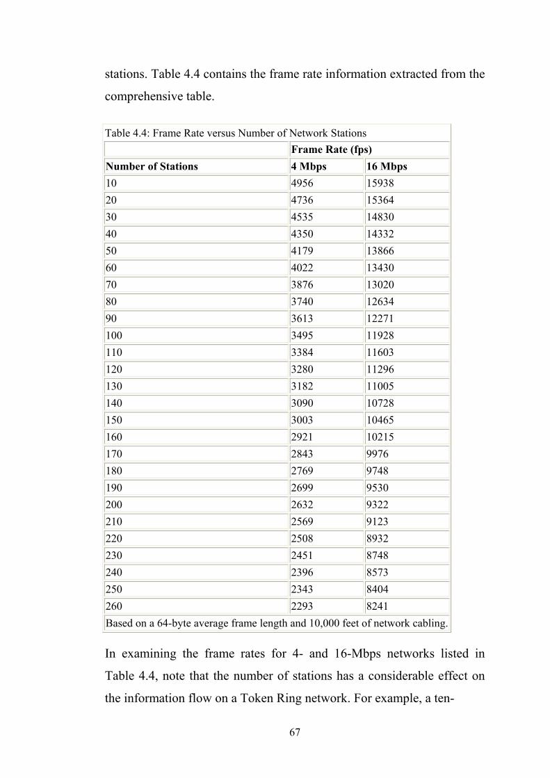
stations. Table 4.4 contains the frame rate information extracted from the
comprehensive table.
Table 4.4: Frame Rate versus Number of Network Stations Frame Rate (fps) Number of Stations 4 Mbps 16 Mbps 10 4956 15938 20 4736 15364 30 4535 14830 40 4350 14332 50 4179 13866 60 4022 13430 70 3876 13020 80 3740 12634 90 3613 12271 100 3495 11928 110 3384 11603 120 3280 11296 130 3182 11005 140 3090 10728 150 3003 10465 160 2921 10215 170 2843 9976 180 2769 9748 190 2699 9530 200 2632 9322 210 2569 9123 220 2508 8932 230 2451 8748 240 2396 8573 250 2343 8404 260 2293 8241 Based on a 64-byte average frame length and 10,000 feet of network cabling.
In examining the frame rates for 4- and 16-Mbps networks listed in
Table 4.4, note that the number of stations has a considerable effect on
the information flow on a Token Ring network. For example, a ten-
67
station 4-Mbps network supports a frame rate of 4956 frames per second,
which is equivalent to an information transfer rate of 4956
frames/second * 64 bytes/frame * 8 bits/byte, or 2.537 Mbps. For a 260-
station network, the frame rate is reduced to 2293 frames per second,
which is equivalent to an information transfer rate of 2293
frames/second * 64 bytes/frame * 8 bits/byte, or 1.174 Mbps. For a 16-
Mbps Token Ring network, note that a ten-station network supports an
information flow of 15,938 frames/second * 64 bytes/frame * 8 bits/byte,
or 8.16 Mbps. When the number of stations is increased to 260, the
information rate decreases to 8241 frames/second * 64 bytes/frame * 8
bits/byte, or 4.219 Mbps. Although the primary reason a Token Ring
network supports a maximum of 260 network stations is based on jitter
of the bits flowing on the network, the approximate halving of the
information transfer capability is another important consideration for
limiting the number of stations on a network this means number of
stations is very important factor for token ring LAN performance.
68
Chapter Five
Simulation of CSMA/CD LANs
Chapter Five Simulation of CSMA/CD LANs
Ethernet is the popular and widely used local area network (LAN).
It is based upon CSMA/CD which is a multiple access protocol. In this
technique, all stations attached to the LAN make their transmission
decisions on the basis of the status of the transmission medium (busy or
idle) as they see it at their interfaces. The transmissions initiated by
various stations may overlap and may cause a collision. This necessitates
retransmission of all collided packets of information. In this chapter, we
discuss simulation of LANs that use CSMA/CD as an access protocol to
measure it's performance by calculating the delay, throughput and
utilization.
5.1 Simulation Model
In this section, we describe the model developed for simulating
CSMA/CD local area networks. The simulation program is written in
turbo C and is based upon the event-scheduling approach. It is self-
driven and needs generation of random numbers according to a desired
probability distribution function. For this purpose, we have used a built-
in function rand(). This function generates uniformly distributed
numbers, which are then converted to follow a desired probability
distribution. In this simulation program, we primarily need exponentially
distributed random numbers. The output of the rand() function can easily
be converted to exponentially distributed numbers using the transform
method.
69
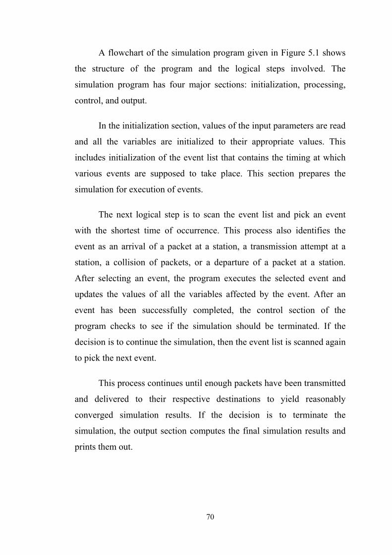
A flowchart of the simulation program given in Figure 5.1 shows
the structure of the program and the logical steps involved. The
simulation program has four major sections: initialization, processing,
control, and output.
In the initialization section, values of the input parameters are read
and all the variables are initialized to their appropriate values. This
includes initialization of the event list that contains the timing at which
various events are supposed to take place. This section prepares the
simulation for execution of events.
The next logical step is to scan the event list and pick an event
with the shortest time of occurrence. This process also identifies the
event as an arrival of a packet at a station, a transmission attempt at a
station, a collision of packets, or a departure of a packet at a station.
After selecting an event, the program executes the selected event and
updates the values of all the variables affected by the event. After an
event has been successfully completed, the control section of the
program checks to see if the simulation should be terminated. If the
decision is to continue the simulation, then the event list is scanned again
to pick the next event.
This process continues until enough packets have been transmitted
and delivered to their respective destinations to yield reasonably
converged simulation results. If the decision is to terminate the
simulation, the output section computes the final simulation results and
prints them out.
70
Figure 5.1 Flow chart of the simulation program.
In this simulation program each packet carries with it a unique
identification number. The number is assigned to a packet as soon as it
arrives at station and remains with the packet until the packet departs
from the network. This identification number is in all calculations related
to a packet. For example, the packet delay is calculated by using the
simulation clock value at the departure time and the start time of a
packet. When a packet is departing, we can find its start time by looking
at its identification number and the starting time associated with that
71
identification number. This approach becomes very helpful when there is
a large number of parameters associated with a packet.
5.1.1 Assumptions:
The following assumptions have been made in the simulation process of
CSMA/CD local area networks:
• Arrivals at all stations follow a Poisson process.
• All stations generate the traffic at the same rate.
• Packet lengths are fixed.
• The transmission medium is assumed to be error-free, and any
errors are only due to collisions.
• The spacing between stations is the same.
• The propagation delay is about 5 microseconds per kilometer of
transmission medium.
5.1.2 Input and Output Variables
Input variables:
MAX_STATIONS
Number of stations in the local area network.
BUS_RATE
Transmission rate of the transmission medium in bits per second. A
reasonable value is from 1.0 Mbps to 10.0 Mbps.
PACKET_LENGTH
Packet length in bits. Its reasonable value is from 500 bits to 10,000
bits.
72
BUS_LENGTH
Length of the transmission medium in meters. This is also used to
compute the end-to-end propagation delay by assuming that the
propagation delay is 5 microseconds per kilometer. A reasonable
value for this variable is 1 km to 5 km.
MAX_BACKOFF
Maximum length of the backoff interval in terms of number of slots. A
reasonable value for this variable is 5.0 to 20.0.
PERSIST
The persistent parameter. This may vary, from 0 to 1 (inclusive). If it is
zero, it represents nonpersistent CSMA/CD; other values represent p-
persistent CSMA/CD.
JAM_PERIOD
The duration of the jamming signal in terms of number of slots. A
reasonable value for this variable is 5.0 to 20.0.
MAX_PACKETS
The number of packets for which each simulation run is executed
before terminating. At lower traffic loads a value of about 5,000 can be
used. However, at higher loads a value of at least 20,000 should be
used. Also, if the size of the network grows, this value should be
increased, too. Basically, this parameter is for convergence of
simulation results.
FACTOR
An accuracy parameter that determines the unit of time for a
simulation run. At higher transmission rates this parameter should
have a higher value for the reasons of accuracy. If FACTOR = 1.0, the
time unit is in seconds. If FACTOR = 1,000, the time unit is
milliseconds, and so on. For our simulation the value of FACTOR
should be at least 1,000.
73
MAX_Q_SIZE
The maximum buffer size at a station. Its reasonable value is from 100
to 500.
ID_SIZE
The size of the identification array. Its reasonable value is about
5,000.
DEGREES_FR
The number of degrees of freedom to be used for calculating
confidence intervals for the output results. In our simulation the range
for this variable is from 1 to 10. However, in most of the results, we
have used 5 degrees of freedom and 95% level of confidence.
Output Variables:
average_delay
The average delay per packet in seconds per packet.
delay_con_int
The 95% confidence interval for the average delay with the selected
degrees of freedom.
utilization
The fraction of time the transmission medium is utilized.
utilization_con_int
The 95% confidence interval for the utilization with a given number of
degrees of freedom.
throughput
The average throughput in terms of packets per second.
collision_rate
The collision rate in terms of collisions per second.
74
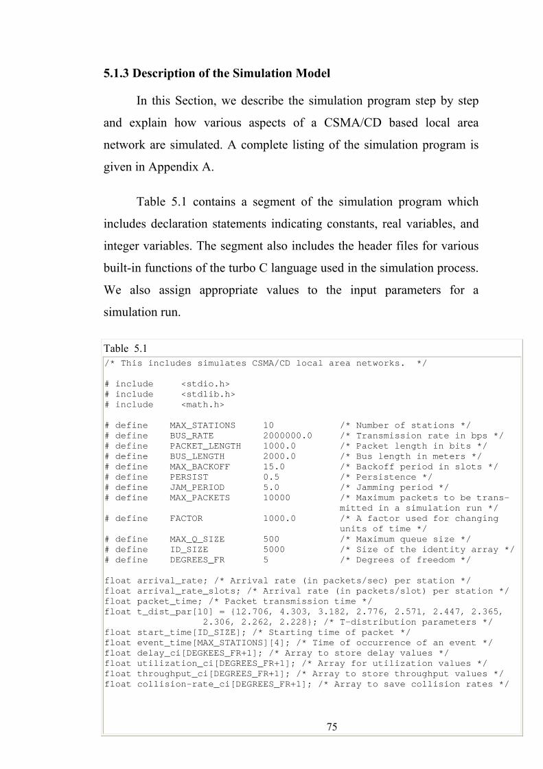
5.1.3 Description of the Simulation Model
In this Section, we describe the simulation program step by step
and explain how various aspects of a CSMA/CD based local area
network are simulated. A complete listing of the simulation program is
given in Appendix A.
Table 5.1 contains a segment of the simulation program which
includes declaration statements indicating constants, real variables, and
integer variables. The segment also includes the header files for various
built-in functions of the turbo C language used in the simulation process.
We also assign appropriate values to the input parameters for a
simulation run.
Table 5.1 /* This includes simulates CSMA/CD local area networks. */ # include <stdio.h> # include <stdlib.h> # include <math.h> # define MAX_STATIONS 10 /* Number of stations */ # define BUS_RATE 2000000.0 /* Transmission rate in bps */ # define PACKET_LENGTH 1000.0 /* Packet length in bits */ # define BUS_LENGTH 2000.0 /* Bus length in meters */ # define MAX_BACKOFF 15.0 /* Backoff period in slots */ # define PERSIST 0.5 /* Persistence */ # define JAM_PERIOD 5.0 /* Jamming period */ # define MAX_PACKETS 10000 /* Maximum packets to be trans- mitted in a simulation run */ # define FACTOR 1000.0 /* A factor used for changing units of time */ # define MAX_Q_SIZE 500 /* Maximum queue size */ # define ID_SIZE 5000 /* Size of the identity array */ # define DEGREES_FR 5 /* Degrees of freedom */ float arrival_rate; /* Arrival rate (in packets/sec) per station */ float arrival_rate_slots; /* Arrival rate (in packets/slot) per station */ float packet_time; /* Packet transmission time */ float t_dist_par[10] = {12.706, 4.303, 3.182, 2.776, 2.571, 2.447, 2.365, 2.306, 2.262, 2.228}; /* T-distribution parameters */ float start_time[ID_SIZE]; /* Starting time of packet */ float event_time[MAX_STATIONS][4]; /* Time of occurrence of an event */ float delay_ci[DEGKEES_FR+1]; /* Array to store delay values */ float utilization_ci[DEGREES_FR+1]; /* Array for utilization values */ float throughput_ci[DEGREES_FR+1]; /* Array to store throughput values */ float collision-rate_ci[DEGREES_FR+1]; /* Array to save collision rates */
75
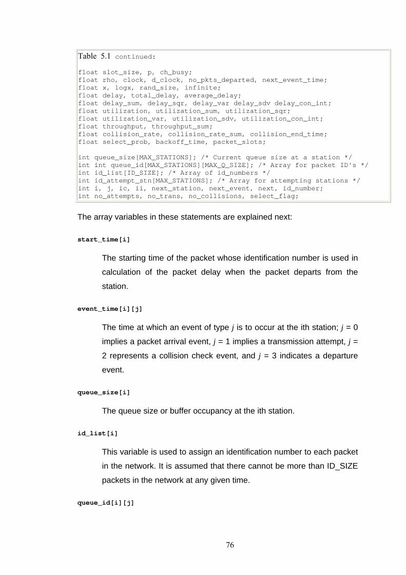
Table 5.1 continued: float slot_size, p, ch_busy; float rho, clock, d_clock, no_pkts_departed, next_event_time; float x, logx, rand_size, infinite; float delay, total_delay, average_delay; float delay_sum, delay_sqr, delay_var delay_sdv delay_con_int; float utilization, utilization_sum, utilization_sqr; float utilization_var, utilization_sdv, utilization_con_int; float throughput, throughput_sum; float collision_rate, collision_rate_sum, collision_end_time; float select_prob, backoff_time, packet_slots; int queue_size[MAX_STATIONS]; /* Current queue size at a station */ int int queue_id[MAX_STATIONS][MAX_Q_SIZE]; /* Array for packet ID's */ int id_list[ID_SIZE]; /* Array of id_numbers */ int id_attempt_stn[MAX_STATIONS]; /* Array for attempting stations */ int i, j, ic, ii, next_station, next_event, next, id_number; int no_attempts, no_trans, no_collisions, select_flag;
The array variables in these statements are explained next:
start_time[i]
The starting time of the packet whose identification number is used in
calculation of the packet delay when the packet departs from the
station.
event_time[i][j]
The time at which an event of type j is to occur at the ith station; j = 0
implies a packet arrival event, j = 1 implies a transmission attempt, j =
2 represents a collision check event, and j = 3 indicates a departure
event.
queue_size[i]
The queue size or buffer occupancy at the ith station.
id_list[i]
This variable is used to assign an identification number to each packet
in the network. It is assumed that there cannot be more than ID_SIZE
packets in the network at any given time.
queue_id[i][j]
76
The identification number of the packet that is sitting in the buffer of
the ith station and occupies the jth position. It is assumed that the
buffer size dose not exceed MAX_Q_SIZE.
t_dist_par[i]
This array contains T-distribution parameters used in calculation of
confidence intervals. The ith element of this array indicates the
parameters to be used in calculating 95% confidence intervals with i
degrees of freedom.
delay_ci[i]
This array is used to temporarily hold the values of delay from various
simulation runs with the same input parameters. These values are
eventually used in calculating confidence intervals.
utilization_ci[i]
This array is used to temporarily hold the values of utilization from
various simulation runs with the same input parameters. These values
are eventually used in calculating confidence intervals.
throughput_ci[i]
This array is used to temporarily hold the values of throughput from
various simulation runs with the same input parameters. These values
may eventually be used in calculation of confidence intervals.
collision_rate_ci[i]
This array is used to temporarily hold the values of collision rate from
various simulation runs with the same input parameters. These values
may eventually be used in calculating confidence intervals.
The segment in Table 5.2 marks the beginning of the main body of the
simulation program. The variable arrival_rate is initialized to zero, and its
value is incremented within a for-loop. Some of the input variables that are
assigned one type of unit in the beginning are converted to a convenient type
77
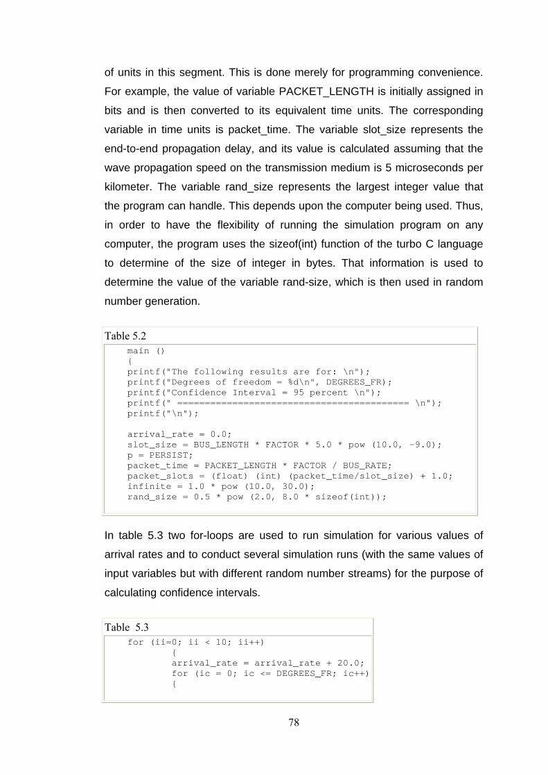
of units in this segment. This is done merely for programming convenience.
For example, the value of variable PACKET_LENGTH is initially assigned in
bits and is then converted to its equivalent time units. The corresponding
variable in time units is packet_time. The variable slot_size represents the
end-to-end propagation delay, and its value is calculated assuming that the
wave propagation speed on the transmission medium is 5 microseconds per
kilometer. The variable rand_size represents the largest integer value that
the program can handle. This depends upon the computer being used. Thus,
in order to have the flexibility of running the simulation program on any
computer, the program uses the sizeof(int) function of the turbo C language
to determine of the size of integer in bytes. That information is used to
determine the value of the variable rand-size, which is then used in random
number generation.
Table 5.2 main () { printf("The following results are for: \n"); printf("Degrees of freedom = %d\n", DEGREES_FR); printf("Confidence Interval = 95 percent \n"); printf(" ========================================== \n"); printf("\n"); arrival_rate = 0.0; slot_size = BUS_LENGTH * FACTOR * 5.0 * pow (10.0, -9.0); p = PERSIST; packet_time = PACKET_LENGTH * FACTOR / BUS_RATE; packet_slots = (float) (int) (packet_time/slot_size) + 1.0; infinite = 1.0 * pow (10.0, 30.0); rand_size = 0.5 * pow (2.0, 8.0 * sizeof(int));
In table 5.3 two for-loops are used to run simulation for various values of
arrival rates and to conduct several simulation runs (with the same values of
input variables but with different random number streams) for the purpose of
calculating confidence intervals.
Table 5.3 for (ii=0; ii < 10; ii++) { arrival_rate = arrival_rate + 20.0; for (ic = 0; ic <= DEGREES_FR; ic++) {
78
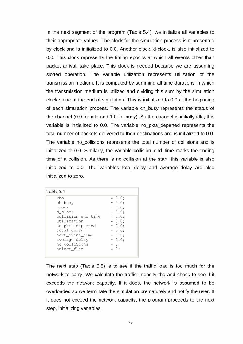
In the next segment of the program (Table 5.4), we initialize all variables to
their appropriate values. The clock for the simulation process is represented
by clock and is initialized to 0.0. Another clock, d-clock, is also initialized to
0.0. This clock represents the timing epochs at which all events other than
packet arrival, take place. This clock is needed because we are assuming
slotted operation. The variable utilization represents utilization of the
transmission medium. It is computed by summing all time durations in which
the transmission medium is utilized and dividing this sum by the simulation
clock value at the end of simulation. This is initialized to 0.0 at the beginning
of each simulation process. The variable ch_busy represents the status of
the channel (0.0 for idle and 1.0 for busy). As the channel is initially idle, this
variable is initialized to 0.0. The variable no_pkts_departed represents the
total number of packets delivered to their destinations and is initialized to 0.0.
The variable no_collisions represents the total number of collisions and is
initialized to 0.0. Similarly, the variable collision_end_time marks the ending
time of a collision. As there is no collision at the start, this variable is also
initialized to 0.0. The variables total_delay and average_delay are also
initialized to zero.
Table 5.4 rho = 0.0; ch_busy = 0.0; clock = 0.0; d_clock = 0.0; collision_end_time = 0.0; utilization = 0.0; no_pkts_departed = 0.0; total_delay = 0.0; next_event_time = 0.0; average_delay = 0.0; no_colliSions = 0; select_flag = 0;
The next step (Table 5.5) is to see if the traffic load is too much for the
network to carry. We calculate the traffic intensity rho and check to see if it
exceeds the network capacity. If it does, the network is assumed to be
overloaded so we terminate the simulation prematurely and notify the user. If
it does not exceed the network capacity, the program proceeds to the next
step, initializing variables.
79
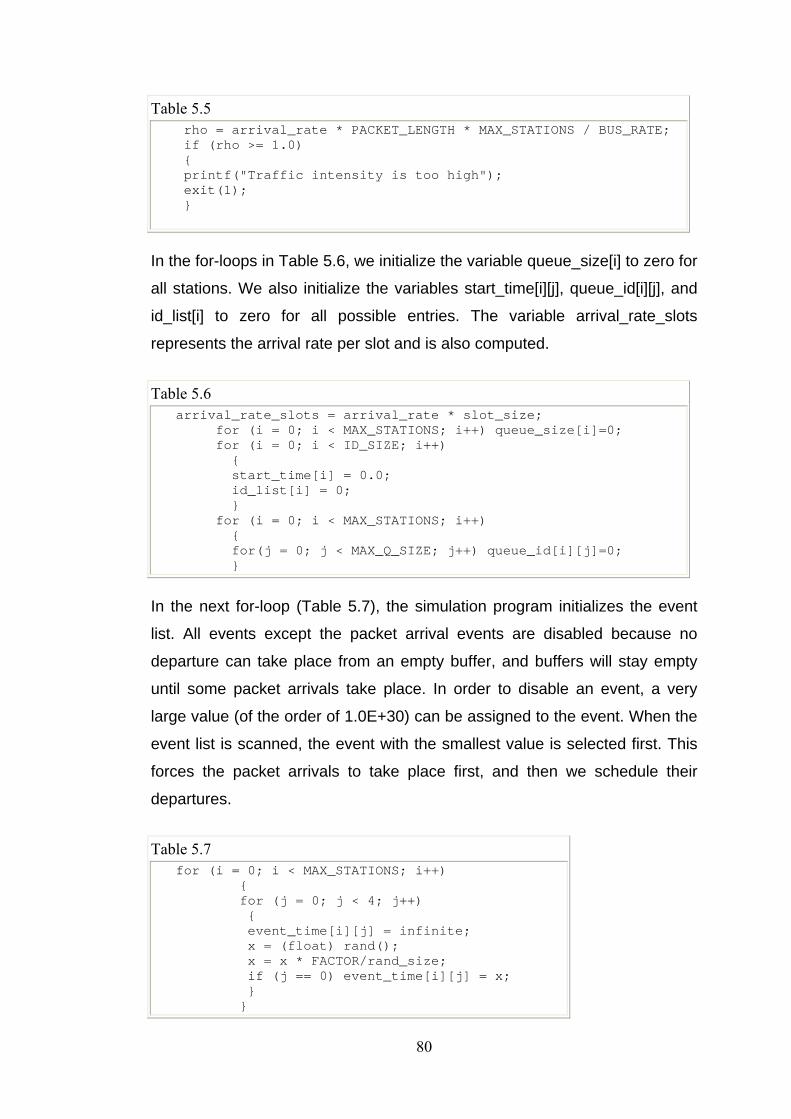
Table 5.5 rho = arrival_rate * PACKET_LENGTH * MAX_STATIONS / BUS_RATE; if (rho >= 1.0) { printf("Traffic intensity is too high"); exit(1); }
In the for-loops in Table 5.6, we initialize the variable queue_size[i] to zero for
all stations. We also initialize the variables start_time[i][j], queue_id[i][j], and
id_list[i] to zero for all possible entries. The variable arrival_rate_slots
represents the arrival rate per slot and is also computed.
Table 5.6 arrival_rate_slots = arrival_rate * slot_size; for (i = 0; i < MAX_STATIONS; i++) queue_size[i]=0; for (i = 0; i < ID_SIZE; i++) { start_time[i] = 0.0; id_list[i] = 0; } for (i = 0; i < MAX_STATIONS; i++) { for(j = 0; j < MAX_Q_SIZE; j++) queue_id[i][j]=0; }
In the next for-loop (Table 5.7), the simulation program initializes the event
list. All events except the packet arrival events are disabled because no
departure can take place from an empty buffer, and buffers will stay empty
until some packet arrivals take place. In order to disable an event, a very
large value (of the order of 1.0E+30) can be assigned to the event. When the
event list is scanned, the event with the smallest value is selected first. This
forces the packet arrivals to take place first, and then we schedule their
departures.
Table 5.7 for (i = 0; i < MAX_STATIONS; i++) { for (j = 0; j < 4; j++) { event_time[i][j] = infinite; x = (float) rand(); x = x * FACTOR/rand_size; if (j == 0) event_time[i][j] = x; } }
80
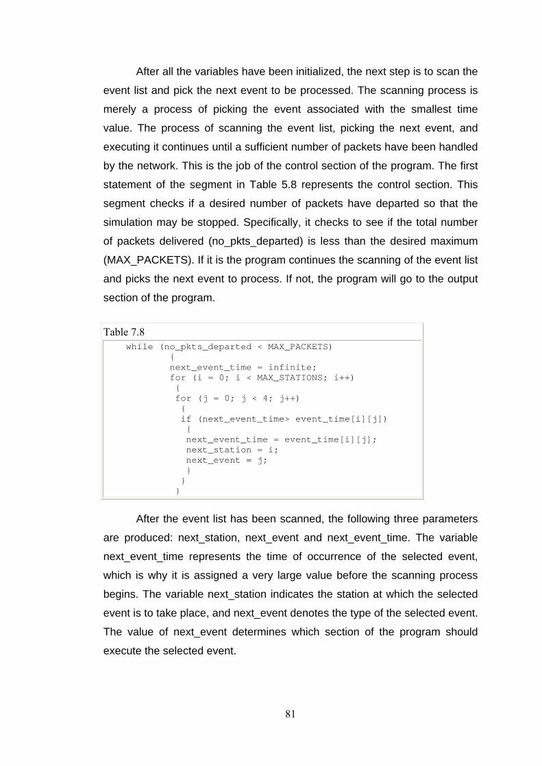
After all the variables have been initialized, the next step is to scan the
event list and pick the next event to be processed. The scanning process is
merely a process of picking the event associated with the smallest time
value. The process of scanning the event list, picking the next event, and
executing it continues until a sufficient number of packets have been handled
by the network. This is the job of the control section of the program. The first
statement of the segment in Table 5.8 represents the control section. This
segment checks if a desired number of packets have departed so that the
simulation may be stopped. Specifically, it checks to see if the total number
of packets delivered (no_pkts_departed) is less than the desired maximum
(MAX_PACKETS). If it is the program continues the scanning of the event list
and picks the next event to process. If not, the program will go to the output
section of the program.
Table 7.8 while (no_pkts_departed < MAX_PACKETS) { next_event_time = infinite; for (i = 0; i < MAX_STATIONS; i++) { for (j = 0; j < 4; j++) { if (next_event_time> event_time[i][j]) { next_event_time = event_time[i][j]; next_station = i; next_event = j; } } }
After the event list has been scanned, the following three parameters
are produced: next_station, next_event and next_event_time. The variable
next_event_time represents the time of occurrence of the selected event,
which is why it is assigned a very large value before the scanning process
begins. The variable next_station indicates the station at which the selected
event is to take place, and next_event denotes the type of the selected event.
The value of next_event determines which section of the program should
execute the selected event.
81
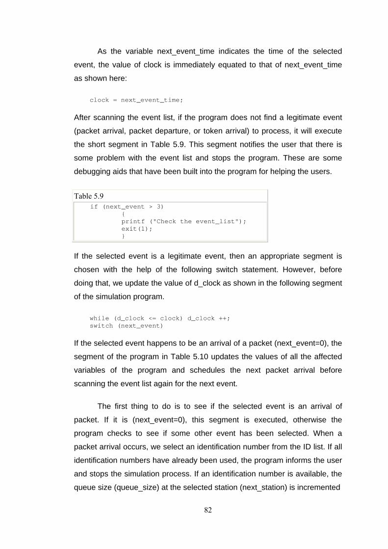
As the variable next_event_time indicates the time of the selected
event, the value of clock is immediately equated to that of next_event_time
as shown here:
clock = next_event_time;
After scanning the event list, if the program does not find a legitimate event
(packet arrival, packet departure, or token arrival) to process, it will execute
the short segment in Table 5.9. This segment notifies the user that there is
some problem with the event list and stops the program. These are some
debugging aids that have been built into the program for helping the users.
Table 5.9 if (next_event > 3) { printf ("Check the event_list"); exit(1); }
If the selected event is a legitimate event, then an appropriate segment is
chosen with the help of the following switch statement. However, before
doing that, we update the value of d_clock as shown in the following segment
of the simulation program.
while (d_clock <= clock) d_clock ++; switch (next_event)
If the selected event happens to be an arrival of a packet (next_event=0), the
segment of the program in Table 5.10 updates the values of all the affected
variables of the program and schedules the next packet arrival before
scanning the event list again for the next event.
The first thing to do is to see if the selected event is an arrival of
packet. If it is (next_event=0), this segment is executed, otherwise the
program checks to see if some other event has been selected. When a
packet arrival occurs, we select an identification number from the ID list. If all
identification numbers have already been used, the program informs the user
and stops the simulation process. If an identification number is available, the
queue size (queue_size) at the selected station (next_station) is incremented
82
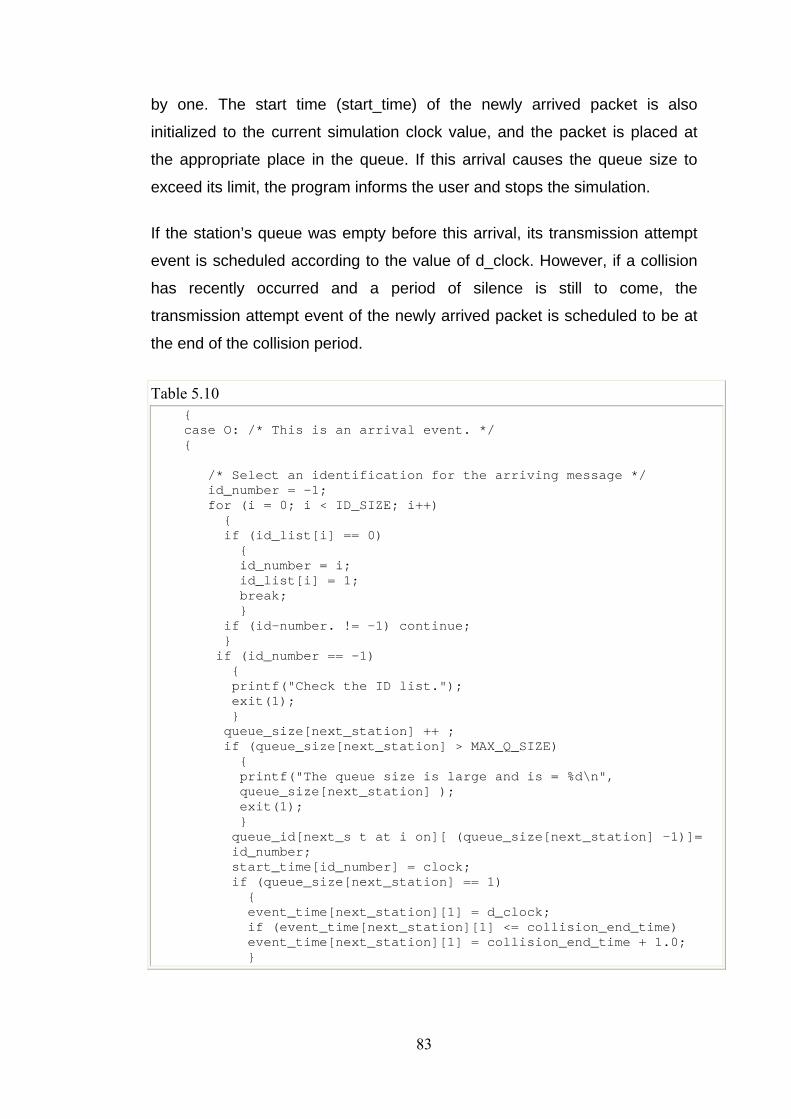
by one. The start time (start_time) of the newly arrived packet is also
initialized to the current simulation clock value, and the packet is placed at
the appropriate place in the queue. If this arrival causes the queue size to
exceed its limit, the program informs the user and stops the simulation.
If the station’s queue was empty before this arrival, its transmission attempt
event is scheduled according to the value of d_clock. However, if a collision
has recently occurred and a period of silence is still to come, the
transmission attempt event of the newly arrived packet is scheduled to be at
the end of the collision period.
Table 5.10 { case O: /* This is an arrival event. */ { /* Select an identification for the arriving message */ id_number = -1; for (i = 0; i < ID_SIZE; i++) { if (id_list[i] == 0) { id_number = i; id_list[i] = 1; break; } if (id-number. != -1) continue; } if (id_number == -1) { printf("Check the ID list."); exit(1); } queue_size[next_station] ++ ; if (queue_size[next_station] > MAX_Q_SIZE) { printf("The queue size is large and is = %d\n", queue_size[next_station] ); exit(1); } queue_id[next_s t at i on][ (queue_size[next_station] -1)]= id_number; start_time[id_number] = clock; if (queue_size[next_station] == 1) { event_time[next_station][1] = d_clock; if (event_time[next_station][1] <= collision_end_time) event_time[next_station][1] = collision_end_time + 1.0; }
83
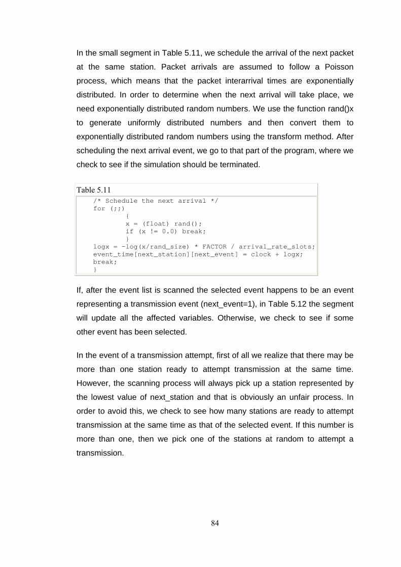
In the small segment in Table 5.11, we schedule the arrival of the next packet
at the same station. Packet arrivals are assumed to follow a Poisson
process, which means that the packet interarrival times are exponentially
distributed. In order to determine when the next arrival will take place, we
need exponentially distributed random numbers. We use the function rand()x
to generate uniformly distributed numbers and then convert them to
exponentially distributed random numbers using the transform method. After
scheduling the next arrival event, we go to that part of the program, where we
check to see if the simulation should be terminated.
Table 5.11 /* Schedule the next arrival */ for (;;) { x = (float) rand(); if (x != 0.0) break; } logx = -log(x/rand_size) * FACTOR / arrival_rate_slots; event_time[next_station][next_event] = clock + logx; break; }
If, after the event list is scanned the selected event happens to be an event
representing a transmission event (next_event=1), in Table 5.12 the segment
will update all the affected variables. Otherwise, we check to see if some
other event has been selected.
In the event of a transmission attempt, first of all we realize that there may be
more than one station ready to attempt transmission at the same time.
However, the scanning process will always pick up a station represented by
the lowest value of next_station and that is obviously an unfair process. In
order to avoid this, we check to see how many stations are ready to attempt
transmission at the same time as that of the selected event. If this number is
more than one, then we pick one of the stations at random to attempt a
transmission.
84
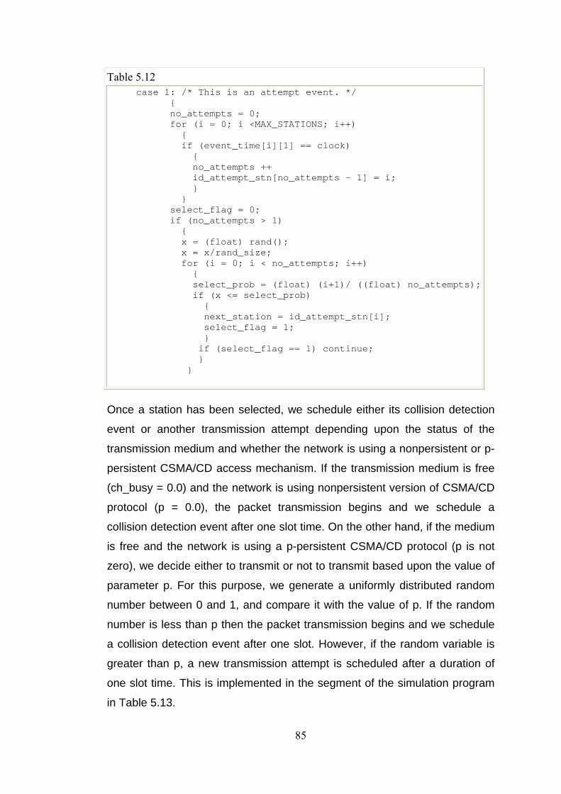
Table 5.12 case 1: /* This is an attempt event. */ { no_attempts = 0; for (i = 0; i <MAX_STATIONS; i++) { if (event_time[i][1] == clock) { no_attempts ++ id_attempt_stn[no_attempts - 1] = i; } } select_flag = 0; if (no_attempts > 1) { x = (float) rand(); x = x/rand_size; for (i = 0; i < no_attempts; i++) { select_prob = (float) (i+1)/ ((float) no_attempts); if (x <= select_prob) { next_station = id_attempt_stn[i]; select_flag = 1; } if (select_flag == 1) continue; } }
Once a station has been selected, we schedule either its collision detection
event or another transmission attempt depending upon the status of the
transmission medium and whether the network is using a nonpersistent or p-
persistent CSMA/CD access mechanism. If the transmission medium is free
(ch_busy = 0.0) and the network is using nonpersistent version of CSMA/CD
protocol (p = 0.0), the packet transmission begins and we schedule a
collision detection event after one slot time. On the other hand, if the medium
is free and the network is using a p-persistent CSMA/CD protocol (p is not
zero), we decide either to transmit or not to transmit based upon the value of
parameter p. For this purpose, we generate a uniformly distributed random
number between 0 and 1, and compare it with the value of p. If the random
number is less than p then the packet transmission begins and we schedule
a collision detection event after one slot. However, if the random variable is
greater than p, a new transmission attempt is scheduled after a duration of
one slot time. This is implemented in the segment of the simulation program
in Table 5.13.
85
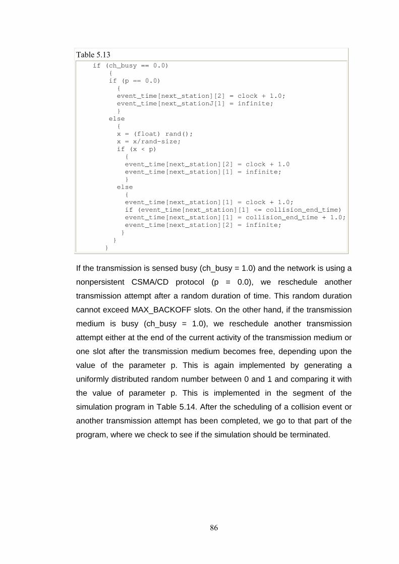
Table 5.13 if (ch_busy == 0.0) { if (p == 0.0) { event_time[next_station][2] = clock + 1.0; event_time[next_stationJ[1] = infinite; } else { x = (float) rand(); x = x/rand-size; if (x < p) { event_time[next_station][2] = clock + 1.0 event_time[next_station][1] = infinite; } else { event_time[next_station][1] = clock + 1.0; if (event_time[next_station][1] <= collision_end_time) event_time[next_station][1] = collision_end_time + 1.0; event_time[next_station][2] = infinite; } } }
If the transmission is sensed busy (ch_busy = 1.0) and the network is using a
nonpersistent CSMA/CD protocol (p = 0.0), we reschedule another
transmission attempt after a random duration of time. This random duration
cannot exceed MAX_BACKOFF slots. On the other hand, if the transmission
medium is busy (ch_busy = 1.0), we reschedule another transmission
attempt either at the end of the current activity of the transmission medium or
one slot after the transmission medium becomes free, depending upon the
value of the parameter p. This is again implemented by generating a
uniformly distributed random number between 0 and 1 and comparing it with
the value of parameter p. This is implemented in the segment of the
simulation program in Table 5.14. After the scheduling of a collision event or
another transmission attempt has been completed, we go to that part of the
program, where we check to see if the simulation should be terminated.
86

Table 5.14 if (ch_busy == 1.0) { if (p == 0.0) { x = (float) rand(); x = x/rand_size; backoff_time = (float) (int) (x * MAX_BACKOFF); if (backoff_time < 1.0) backoff_time = 1.0; event_time[next_station][1] = clock + backoff_time; if (event_time[next_station][1] <= collision_end_time) event_time[next-station][1] = collision_end_time + backoff_time; event_time[next-station][2] = infinite; } else { event_time[next_station][1] = clock + 1.0; if (event_time[next_station][1] <= collision_end_time) event_time[next-station][1] = collision_end_time + 1.0; event_time[next_station][2] = infinite; } } break; }
In this section (Table 5.15), the program checks to see if a collision has taken
place. The first item is to make sure that the selected event is that of a
collision check (next_event = 2). If it is, we proceed to update all the affected
variables. Initially, we count the number of stations (no_trans) transmitting at
the same time. If no_trans is greater than 1, then there is a collision. In this
case, all transmitting stations must back off, send a jamming signal for a
specified duration of time (JAM_PERIOD), wait for a silence period equal to
two slot times, and schedule their transmission attempts after a random
duration of time. All stations that were attempting to transmit before the
collision occurred must also back off and reschedule their transmission
attempts later. However, if there is no collision (no_trans = 1), the
transmission is successful and the simulation program schedules departure
of the packet. After scheduling the departure, the simulation program checks
to see if the simulation is to be terminated.
87
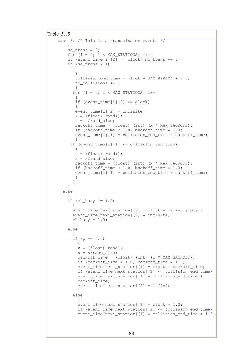
Table 5.15 case 2: /* This is a transmission event, */ { no_trans = 0; for (i = 0; i < MAX_STATIONS; i++) if (event_time[i][2] == clock) no_trans ++ ; if (no_trans > 1) { { collision_end_time = clock + JAM_PERIOD + 2.0; no_collisions ++ ; } for (i = 0; i < MAX_STATIONS; i++) { if (event_time[i][2] == clock) { event time[i][2] = infinite; x = (float) rand(); x = x/rand_size; backoff_time = (float) (int) (x * MAX_BACKOFF); if (backoff_time < 1.0) backoff_time = 1.0; event_time[i][1] = collision_end_time + backoff_time; } if (event_time[i][1] <= collision_end_time) { x = (float) rand(); x = x/rand_size; backoff_time = (float) (int) (x * MAX_BACKOFF); if (backoff_time < 1.0) backoff_time = 1.0; event_time[i][1] = collision_end_time + backoff_time; } } } else { if (ch_busy != 1.0) { event_time[next_station][3] = clock + packet_slots ; event_time[next_station][2] = infinite; ch_busy = 1.0; } else { if (p == 0.0) { x = (float) rand(); x = x/rand_size; backoff_time = (float) (int) (x * MAX_BACKOFF); if (backoff_time < 1.0) backoff_time = 1.0; event_time[next_station][1] = clock + backoff_time; if (event_time[next_station][1] <= collision_end_time) event_time[next_station][1] = collision_end_time + backoff_time; event_time[next_station][2] = infinite; } else { event_time[next_station][1] = clock + 1.0; if (event_time[next_station][1] <= collision_end_time) event_time[next_station][1] = collision_end_time + 1.0;
88
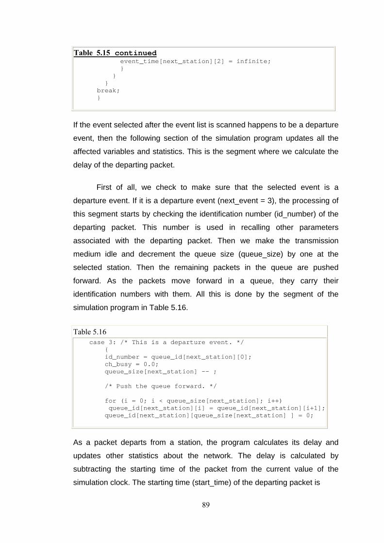
Table 5.15 continued event_time[next_station][2] = infinite; } } } break; }
If the event selected after the event list is scanned happens to be a departure
event, then the following section of the simulation program updates all the
affected variables and statistics. This is the segment where we calculate the
delay of the departing packet.
First of all, we check to make sure that the selected event is a
departure event. If it is a departure event (next_event = 3), the processing of
this segment starts by checking the identification number (id_number) of the
departing packet. This number is used in recalling other parameters
associated with the departing packet. Then we make the transmission
medium idle and decrement the queue size (queue_size) by one at the
selected station. Then the remaining packets in the queue are pushed
forward. As the packets move forward in a queue, they carry their
identification numbers with them. All this is done by the segment of the
simulation program in Table 5.16.
Table 5.16 case 3: /* This is a departure event. */ { id_number = queue_id[next_station][0]; ch_busy = 0.0; queue_size[next_station] -- ; /* Push the queue forward. */ for (i = 0; i < queue_size[next_station]; i++) queue_id[next_station][i] = queue_id[next_station][i+1]; queue_id[next_station][queue_size[next_station] ] = 0;
As a packet departs from a station, the program calculates its delay and
updates other statistics about the network. The delay is calculated by
subtracting the starting time of the packet from the current value of the
simulation clock. The starting time (start_time) of the departing packet is
89
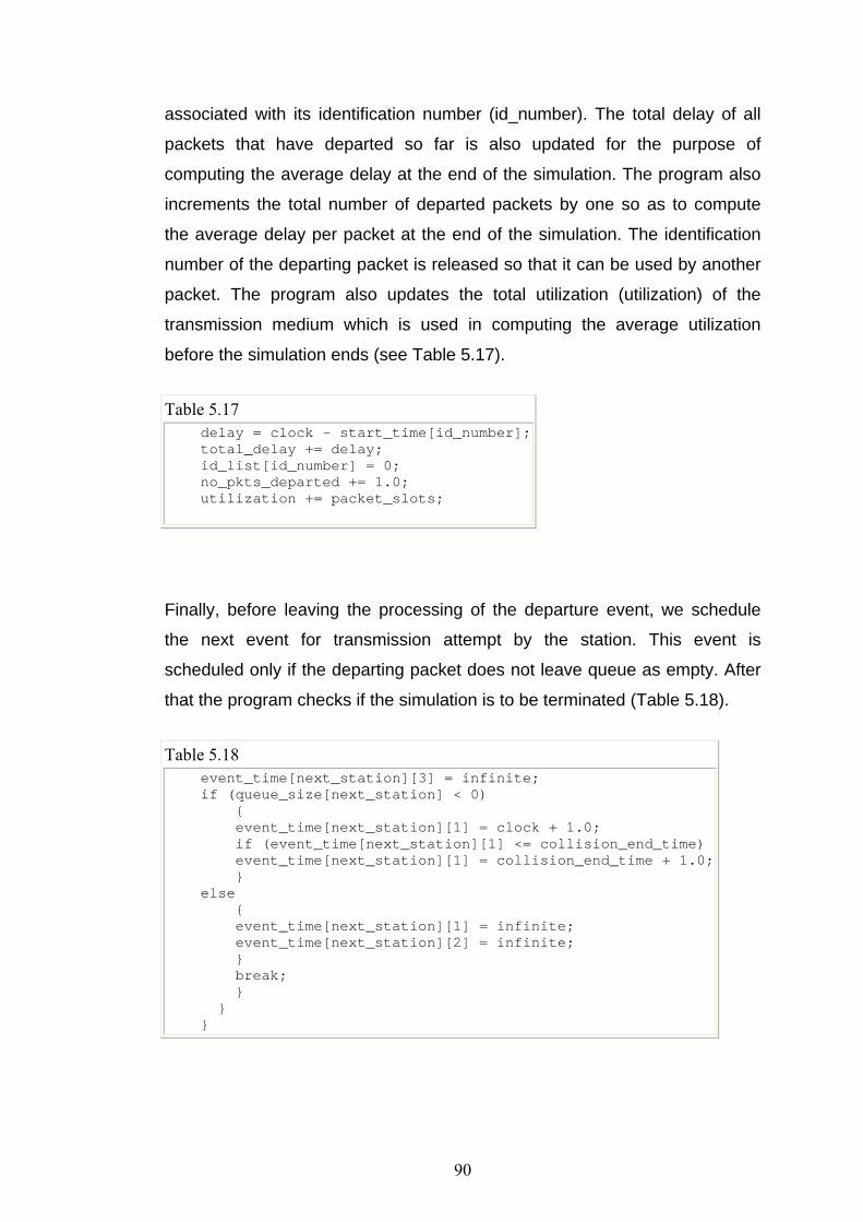
associated with its identification number (id_number). The total delay of all
packets that have departed so far is also updated for the purpose of
computing the average delay at the end of the simulation. The program also
increments the total number of departed packets by one so as to compute
the average delay per packet at the end of the simulation. The identification
number of the departing packet is released so that it can be used by another
packet. The program also updates the total utilization (utilization) of the
transmission medium which is used in computing the average utilization
before the simulation ends (see Table 5.17).
Table 5.17 delay = clock - start_time[id_number]; total_delay += delay; id_list[id_number] = 0; no_pkts_departed += 1.0; utilization += packet_slots;
Finally, before leaving the processing of the departure event, we schedule
the next event for transmission attempt by the station. This event is
scheduled only if the departing packet does not leave queue as empty. After
that the program checks if the simulation is to be terminated (Table 5.18).
Table 5.18 event_time[next_station][3] = infinite; if (queue_size[next_station] < 0) { event_time[next_station][1] = clock + 1.0; if (event_time[next_station][1] <= collision_end_time) event_time[next_station][1] = collision_end_time + 1.0; } else { event_time[next_station][1] = infinite; event_time[next_station][2] = infinite; } break; } } }
90
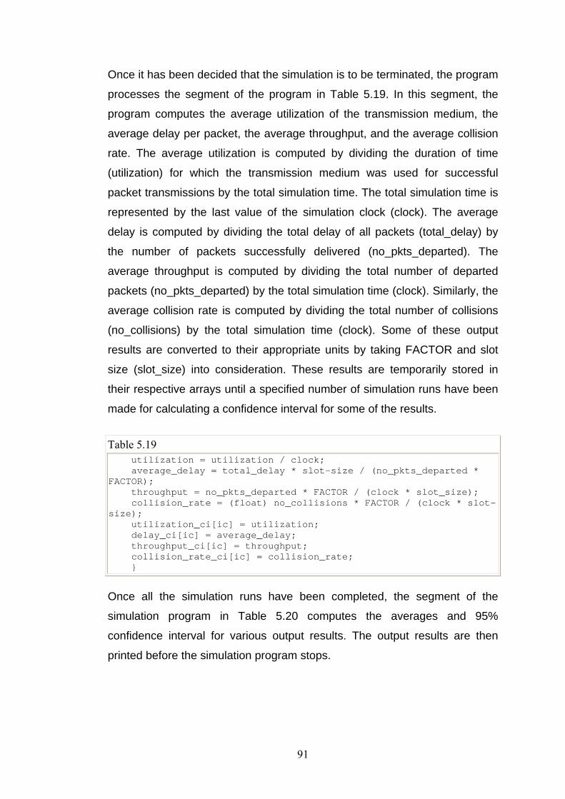
Once it has been decided that the simulation is to be terminated, the program
processes the segment of the program in Table 5.19. In this segment, the
program computes the average utilization of the transmission medium, the
average delay per packet, the average throughput, and the average collision
rate. The average utilization is computed by dividing the duration of time
(utilization) for which the transmission medium was used for successful
packet transmissions by the total simulation time. The total simulation time is
represented by the last value of the simulation clock (clock). The average
delay is computed by dividing the total delay of all packets (total_delay) by
the number of packets successfully delivered (no_pkts_departed). The
average throughput is computed by dividing the total number of departed
packets (no_pkts_departed) by the total simulation time (clock). Similarly, the
average collision rate is computed by dividing the total number of collisions
(no_collisions) by the total simulation time (clock). Some of these output
results are converted to their appropriate units by taking FACTOR and slot
size (slot_size) into consideration. These results are temporarily stored in
their respective arrays until a specified number of simulation runs have been
made for calculating a confidence interval for some of the results.
Table 5.19 utilization = utilization / clock; average_delay = total_delay * slot-size / (no_pkts_departed * FACTOR); throughput = no_pkts_departed * FACTOR / (clock * slot_size); collision_rate = (float) no_collisions * FACTOR / (clock * slot-size); utilization_ci[ic] = utilization; delay_ci[ic] = average_delay; throughput_ci[ic] = throughput; collision_rate_ci[ic] = collision_rate; }
Once all the simulation runs have been completed, the segment of the
simulation program in Table 5.20 computes the averages and 95%
confidence interval for various output results. The output results are then
printed before the simulation program stops.
91
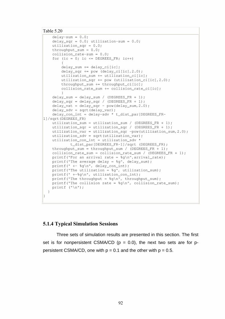
Table 5.20 delay-sum = 0.0; delay_sqr = 0.0; utilization-sum = 0.0; utilization_sqr = 0.0; throughput_sum = 0.0; collision_rate-sum = 0.0; for (ic = 0; ic <= DEGREES_FR; ic++) { delay_sum += delay_ci[ic]; delay_sqr += pow (delay_ci[ic],2.0); utilization_sum += utilization_ci[ic]; utilization_sqr += pow (utilization_ci[ic],2.0); throughput_sum += throughput_ci[ic]; collision_rate_sum += collision_rate_ci[ic]; } delay_sum = delay_sum / (DEGREES_FR + 1); delay_sqr = delay_sqr / (DEGREES_FR + 1); delay_vat = delay_sqr - pow(delay_sum,2.0); delay_sdv = sqrt(delay_var); delay_con_int = delay-sdv * t_dist_par[DEGREES_FR-1]/sqrt(DEGREES_FR) utilization_sum = utilization_sum / (DEGREES_FR + 1); utilization_sqr = utilization_sqr / (DEGREES_FR + 1); utilization_var = utilization_sqr -pow(utilization_sum,2.0); utilization_sdv = sqrt(utilization_var); utilization_con_int = utilization_sdv * t_dist_par[DEGREES_FR-1]/sqrt (DEGREES_FR); throughput_sum = throughput_sum / (DEGREES_FR + 1); collision_rate_sum = collision_rate_sum / (DEGREES_FR + 1); printf("For an arrival rate = %g\n",arrival_rate); printf("The average delay = %g", delay_sum); printf(" +- %g\n", delay_con_int); printf("The utilization = %g", utilization_sum); printf(" +-%g\n", utilization_con_int); printf("The throughput = %g\n", throughput_sum); printf("The collision rate = %g\n", collision_rate_sum); printf ("\n"); } }
5.1.4 Typical Simulation Sessions
Three sets of simulation results are presented in this section. The first
set is for nonpersistent CSMA/CD (p = 0.0), the next two sets are for p-
persistent CSMA/CD, one with p = 0.1 and the other with p = 0.5.
92
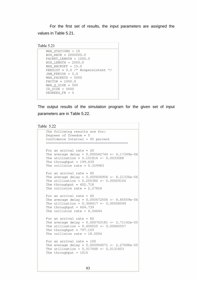
For the first set of results, the input parameters are assigned the
values in Table 5.21.
Table 5.21 MAX_STATIONS = 10 BUS_RATE = 2000000.0 PACKET_LENGTH = 1000.0 BUS_LENGTH = 2000.0 MAX_BACKOFF = 15.0 PERSIST = 0.0 /* Nonpersistent */ JAM_PERIOD = 5.0 MAX_PACKETS = 5000 FACTOR = 1000.0 MAX_Q_SIZE = 500 ID_SIZE = 5000 DEGREES_FR = 5
The output results of the simulation program for the given set of input
parameters are in Table 5.22.
Table 5.22 The following results are for: Degrees of freedom = 5 Confidence Interval = 95 percent ========================================= For an arrival rate = 20 The average delay = 0.000562744 +- 4.17349e-06 The utilization = 0.101816 +- 0.0033588 The throughput = 199.639 The collision rate = 0.329983 For an arrival rate = 40 The average delay = 0.000606906 +- 8.21336e-06 The utilization = 0.205386 +- 0.00509104 The throughput = 402.718 The collision rate = 2.27824 For an arrival rate = 60 The average delay = 0.000672506 +- 8.85559e-06 The utilization = 0.308417 +- 0.00508099 The throughput = 604.739 The collision rate = 6.54644 For an arrival rate = 80 The average delay = 0.000763181 +- 2.71142e-05 The utilization = 0.406525 +- 0.00860557 The throughput = 797.109 The collision rate = 18.5004 For an arrival rate = 100 The average delay = 0.000904571 +- 2.27698e-05 The utilization = 0.517648 +- 0.0131853 The throughput = 1015
93
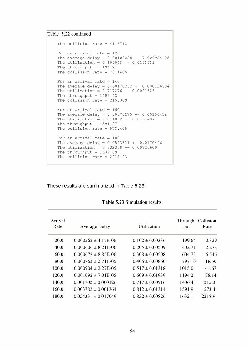
Table 5.22 continued The collision rate = 41.6712 For an arrival rate = 120 The average delay = 0.00109228 +- 7.00992e-05 The utilization = 0.609048 +- 0.0193935 The throughput = 1194.21 The collision rate = 78.1405 For an arrival rate = 140 The average delay = 0.00170232 +- 0.000126584 The utilization = 0.717276 +- 0.0091623 The throughput = 1406.42 The collision rate = 215.309 For an arrival rate = 160 The average delay = 0.00378275 +- 0.00136432 The utilization = 0.811852 +- 0.0131487 The throughput = 1591.87 The collision rate = 573.405 For an arrival rate = 180 The average delay = 0.0543311 +- 0.0170496 The utilization = 0.832368 +- 0.00826609 The throughput = 1632.09 The collision rate = 2218.93
These results are summarized in Table 5.23.
Table 5.23 Simulation results.
Arrival
Rate Average Delay Utilization Through-
put Collision
Rate
20.0 0.000562 ± 4.17E-06 0.102 ± 0.00336 199.64 0.329 40.0 0.000606 ± 8.21E-06 0.205 ± 0.00509 402.71 2.278 60.0 0.000672 ± 8.85E-06 0.308 ± 0.00508 604.73 6.546 80.0 0.000763 ± 2.71E-05 0.406 ± 0.00860 797.10 18.50 100.0 0.000904 ± 2.27E-05 0.517 ± 0.01318 1015.0 41.67 120.0 0.001092 ± 7.01E-05 0.609 ± 0.01939 1194.2 78.14 140.0 0.001702 ± 0.000126 0.717 ± 0.00916 1406.4 215.3 160.0 0.003782 ± 0.001364 0.812 ± 0.01314 1591.9 573.4 180.0 0.054331 ± 0.017049 0.832 ± 0.00826 1632.1 2218.9
94

For simulating p-persistent CSMA/CD LANs, one may give the set of input
parameters in Table 5.24.
Table 5.24 MAX_STATIONS = 10 BUS_RATE = 2000000.0 PACKET_LENGTH = 1000.0 BUS_LENGTH = 2000.0 MAX_BACKOFF = 15.0 PERSIST = 0.1 /* p-Persistent */ JAM_PERIOD = 5.0 MAX_PACKETS = 5000 FACTOR = 1000.0 MAX_Q_SIZE = 500 ID_SIZE = 5000 DEGREES_FR = 5
The output results for this set of parameters are in Table 5.25.
Table 5.25 The following results are for: Degrees of freedom 5 Confidence Interval = 95 percent ========================================== For an arrival rate = 20 The average delay = 0.000658616 +- 3.04385e-06 The utilization = 0.101 +- 0.00172139 The throughput = 198.04 The collision rate = 0.379955 For an arrival rate = 40 The average delay = 0.000715458 +- 4.15925e-06 The utilization = 0.20489 +- 0.00567377 The throughput = 401.745 The collision rate = 1.37544 For an arrival rate = 60 The average delay = 0.000791979 +- 2.07238e-05 The utilization = 0.310382 +- 0.00900632 The throughput = 608.591 The collision rate = 4.93771 For an arrival rate = 80 The average delay = 0.00088773 +- 2.11368e-05 The utilization = 0.407861 +- 0.00824132 The throughput = 799.727 The collision rate = 10.0247 For an arrival rate = 100 The average delay = 0.0010505 +- 1.68148e-05 The utilization = 0.514659 +- 0.0100435 The throughput = 1009.14 The collision rate 25.4778 For an arrival rate = 120
95
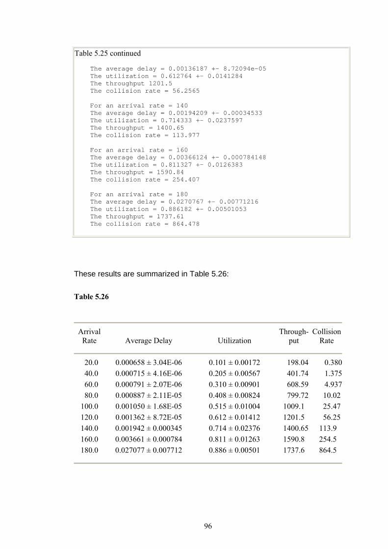
Table 5.25 continued The average delay = 0.00136187 +- 8.72094e-05 The utilization = 0.612764 +- 0.0141284 The throughput 1201.5 The collision rate = 56.2565 For an arrival rate = 140 The average delay = 0.00194209 +- 0.00034533 The utilization = 0.714333 +- 0.0237597 The throughput = 1400.65 The collision rate = 113.977 For an arrival rate = 160 The average delay = 0.00366124 +- 0.000784148 The utilization = 0.811327 +- 0.0126383 The throughput = 1590.84 The collision rate = 254.407 For an arrival rate = 180 The average delay = 0.0270767 +- 0.00771216 The utilization = 0.886182 +- 0.00501053 The throughput = 1737.61 The collision rate = 864.478
These results are summarized in Table 5.26:
Table 5.26
Arrival Rate Average Delay Utilization
Through-put
Collision Rate
20.0 0.000658 ± 3.04E-06 0.101 ± 0.00172 198.04 0.380 40.0 0.000715 ± 4.16E-06 0.205 ± 0.00567 401.74 1.375 60.0 0.000791 ± 2.07E-06 0.310 ± 0.00901 608.59 4.937 80.0 0.000887 ± 2.11E-05 0.408 ± 0.00824 799.72 10.02 100.0 0.001050 ± 1.68E-05 0.515 ± 0.01004 1009.1 25.47 120.0 0.001362 ± 8.72E-05 0.612 ± 0.01412 1201.5 56.25 140.0 0.001942 ± 0.000345 0.714 ± 0.02376 1400.65 113.9 160.0 0.003661 ± 0.000784 0.811 ± 0.01263 1590.8 254.5 180.0 0.027077 ± 0.007712 0.886 ± 0.00501 1737.6 864.5
96
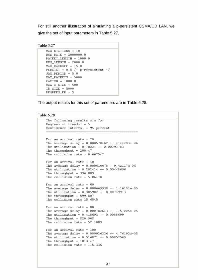
For still another illustration of simulating a p-persistent CSMA/CD LAN, we
give the set of input parameters in Table 5.27.
Table 5.27 MAX_STATIONS = 10 BUS_RATE = 2000000.0 PACKET_LENGTH = 1000.0 BUS_LENGTH = 2000.0 MAX_BACKOFF = 15.0 PERSIST = 0.5 /* p-Persistent */ JAM_PERIOD = 5.0 MAX_PACKETS = 5000 FACTOR = 1000.0 MAX_Q_SIZE = 500 ID_SIZE = 5000 DEGREES_FR = 5
The output results for this set of parameters are in Table 5.28.
Table 5.28 The following results are for: Degrees of freedom = 5 Confidence Interval = 95 percent ============================================== For an arrival rate = 20 The average delay = 0.000570462 +- 4.44283e-06 The utilization = 0.10224 +- 0.00292783 The throughput = 200.47 The collision rate = 0.667547 For an arrival rate = 40 The average delay = 0.000616678 + 9.42117e-06 The utilization = 0.202414 +- 0.00448696 The throughput = 396.889 The collision rate = 5.06478 For an arrival rate = 60 The average delay = 0.000669938 +- 1.16101e-05 The utilization = 0.305902 +- 0.00749913 The throughput = 599.807 The collision rate 15.6545 For an arrival rate = 80 The average delay = 0.000782643 +- 1.57005e-05 The utilization = 0.418693 +- 0.0088699 The throughput = 820.968 The collision rate = 52.1089 For an arrival rate = 100 The average delay = 0.000936336 +- 4.76193e-05 The utilization = 0.516871 +- 0.00857569 The throughput = 1013.47 The collision rate = 115.336
97
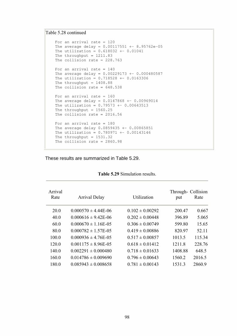
Table 5.28 continued For an arrival rate = 120 The average delay = 0.00117551 +- 8.95762e-05 The utilization = 0.618032 +- 0.01041 The throughput = 1211.83 The collision rate = 228.763 For an arrival rate = 140 The average delay = 0.00229173 +- 0.000480587 The utilization = 0.718528 +- 0.0163306 The throughput = 1408.88 The collision rate = 648.538 For an arrival rate = 160 The average delay = 0.0147868 +- 0.00969014 The utilization = 0.79573 +- 0.00643513 The throughput = 1560.25 The collision rate = 2016.56 For an arrival rate = 180 The average delay 0.0859435 +- 0.00865851 The utilization = 0.780971 +- 0.00143146 The throughput = 1531.32 The collision rate = 2860.98
These results are summarized in Table 5.29.
Table 5.29 Simulation results.
Arrival
Rate Arrival Delay Utilization Through-
put Collision
Rate
20.0 0.000570 ± 4.44E-06 0.102 ± 0.00292 200.47 0.667 40.0 0.000616 ± 9.42E-06 0.202 ± 0.00448 396.89 5.065 60.0 0.000670 ± 1.16E-05 0.306 ± 0.00749 599.80 15.65 80.0 0.000782 ± 1.57E-05 0.419 ± 0.00886 820.97 52.11 100.0 0.000936 ± 4.76E-05 0.517 ± 0.00857 1013.5 115.34 120.0 0.001175 ± 8.96E-05 0.618 ± 0.01412 1211.8 228.76 140.0 0.002291 ± 0.000480 0.718 ± 0.01633 1408.88 648.5 160.0 0.014786 ± 0.009690 0.796 ± 0.00643 1560.2 2016.5 180.0 0.085943 ± 0.008658 0.781 ± 0.00143 1531.3 2860.9
98
Chapter Six
Simulation of Token-Passing LANs
Chapter Six Simulation of Token-Passing LANs
In this chapter, we discuss simulation of token-passing local area
networks (LANs). Token-passing is a technique in which the
transmission medium is shared without conflict among LAN users.
6.1 Simulation Model
In this section, we describe the simulation model developed for
simulating token-passing (ring and bus) local area networks. We have
used the event-scheduling approach in this simulation and it is self-
driven. The program is written in turbo C. Generation of random
numbers according to a desired probability distribution is a necessity for
any self-driven simulation. In this simulation program we have used a
built-in function rand( ) for this purpose. This function generates
uniformly distributed numbers, which are then converted to follow a
desired probability distribution. In this simulation program, we primarily
need exponentially distributed random numbers. The output of the rand(
) function can easily be converted to exponentially distributed numbers
using the transform method.
A flowchart of the simulation program is given in Figure 6.1 that
shows the structure of the program and the logical steps involved. The
simulation program has four major sections: initialization, processing,
control, and output. In the initialization section, values of the input
parameters are read and all the variables are initialized to their
appropriate values. This includes initialization of the event list, which
99
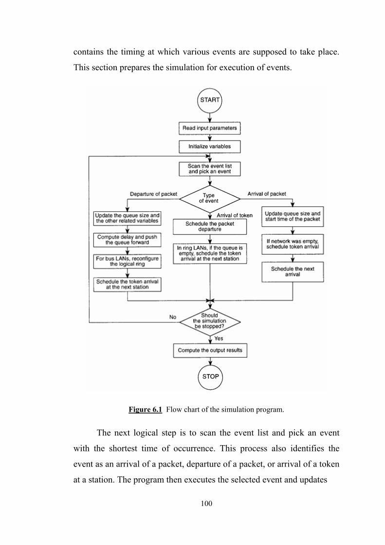
contains the timing at which various events are supposed to take place.
This section prepares the simulation for execution of events.
Figure 6.1 Flow chart of the simulation program.
The next logical step is to scan the event list and pick an event
with the shortest time of occurrence. This process also identifies the
event as an arrival of a packet, departure of a packet, or arrival of a token
at a station. The program then executes the selected event and updates
100
the values of all the variables affected by the event. This is part of the
processing section. After an event has been successfully completed, the
program control section checks to see if the simulation should be
terminated. If the decision is to continue the simulation, then the event
list is scanned again to pick the next event. This process continues until a
sufficient number of packets have been transmitted and delivered to their
respective destinations to yield reasonably converged simulation results.
If the decision is to terminate the simulation, the output section computes
the final simulation results and prints them out, and the simulation
process stops.
6.1.1 Assumptions
The following assumptions have been made in the simulation process:
• Arrivals at all stations follow a Poisson process.
• All stations generate the traffic at the same rate.
• Packet lengths are fixed.
• Multiple token operation has been used.
• The transmission medium is assumed to be error-free.
• The spacing between stations is the same.
• The source and destination stations are on the average half the
ring apart.
• The propagation delay is about five microseconds per kilometer
of transmission medium.
101
6.1.2 Input and Output Variables
Input Variables:
MAX_STATIONS
Number of stations in the local area network.
RING_OR_BUS
This variable is used to choose ring or bus local area network for
simulation. If RING_OR_BUS = 1, the program simulates a ring LAN;
otherwise it simulates a bus LAN.
RATE
Transmission rate of the transmission medium in bits per second. Its
reasonable value is 1.0 Mbps to 5.0 Mbps.
PACKET_LENGTH
Packet length in bits. Its reasonable value is from 500 bits to 10,000
bits.
MEDIUM_LENGTH
Length of the transmission medium in meters. This is also used to
compute the end-to-end propagation delay by assuming that the
propagation delay is 5 microseconds per kilometer. A reasonable
value of this variable is 1 km to 5 km.
TOKEN_LENGTH
Token length in bits. Its typical value is 8 bits for ring LANs and 48 bits
for bus LANs.
STN_LATENCY
Station latency of interfaces. For bus LANs, its value is zero; for ring
LANs, it is typically 1 bit.
MAX_PACKETS
102
The number of packets for which each simulation run is executed
before terminating. At lower traffic loads, a value of about 5,000 can
be used. However, at higher loads a value of at least 20,000 should be
used. Also if the size of the network grows, this value should be
increased, too. Basically this parameter is for convergence of
simulation results.
FACTOR
An accuracy parameter that determines the unit of time for a
simulation run. At higher transmission rates this parameter should
have a higher value for reasons of accuracy. If FACTOR = 1.0, the
time unit is in seconds. If FACTOR = 1,000, the time unit is
milliseconds, and so on. For our simulation the value of FACTOR
should be at least 1,000.
MAX_Q_SIZE
The maximum buffer size at a station.
DEGREES_FR
The degrees of freedom to be used for calculating confidence intervals
for the output results. In our simulation the range for this variable is
from 1 to 10. However, in most of the results, we have used 5 degrees
of freedom and a 95% level of confidence.
Output Variables:
average_delay
The average delay per packet in seconds per packet.
delay_con_int
This variable represents a 95% confidence interval for the average
delay with the selected degrees of freedom.
103
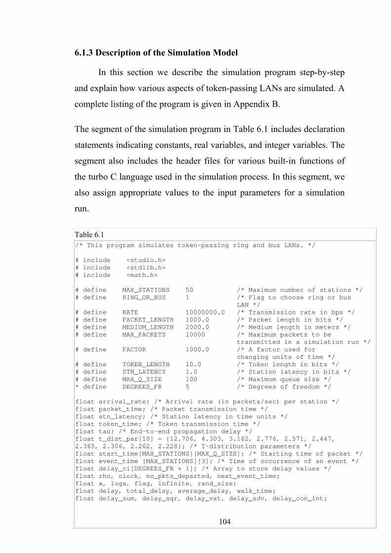
6.1.3 Description of the Simulation Model
In this section we describe the simulation program step-by-step
and explain how various aspects of token-passing LANs are simulated. A
complete listing of the program is given in Appendix B.
The segment of the simulation program in Table 6.1 includes declaration
statements indicating constants, real variables, and integer variables. The
segment also includes the header files for various built-in functions of
the turbo C language used in the simulation process. In this segment, we
also assign appropriate values to the input parameters for a simulation
run.
Table 6.1 /* This program simulates token-passing ring and bus LANs. */ # include <studio.h> # include <stdlib.h> # include <math.h> # define MAX_STATIONS 50 /* Maximum number of stations */ # define RING_OR_BUS 1 /* Flag to choose ring or bus LAN */ # define RATE 10000000.0 /* Transmission rate in bps */ # define PACKET_LENGTH 1000.0 /* Packet length in bits */ # define MEDIUM_LENGTH 2000.0 /* Medium length in meters */ # define MAX_PACKETS 10000 /* Maximum packets to be transmitted in a simulation run */ # define FACTOR 1000.0 /* A factor used for changing units of time */ # define TOKEN_LENGTH 10.0 /* Token length in bits */ # define STN_LATENCY 1.0 /* Station latency in bits */ # define MAX_Q_SIZE 100 /* Maximum queue size */ * define DEGREES_FR 5 /* Degrees of freedom */ float arrival_rate; /* Arrival rate (in packets/sec) per station */ float packet_time; /* Packet transmission time */ float stn_latency; /* Station latency in time units */ float token_time; /* Token transmission time */ float tau; /* End-to-end propagation delay */ float t_dist_par[10] = {12.706, 4.303, 3.182, 2.776, 2.571, 2.447, 2.365, 2.306, 2.262, 2.228}; /* T-distribution parameters */ float start_time[MAX_STATIONS][MAX_Q_SIZE]; /* Starting time of packet */ float event_time [MAX_STATIONS][3]; /* Time of occurrence of an event */ float delay_ci[DEGREES_FR + 1]; /* Array to store delay values */ float rho, clock, no_pkts_departed, next_event_time; float x, logx, flag, infinite, rand_size; float delay, total_delay, average_delay, walk_time; float delay_sum, delay_sqr, delay_vat, delay_sdv, delay_con_int;
104
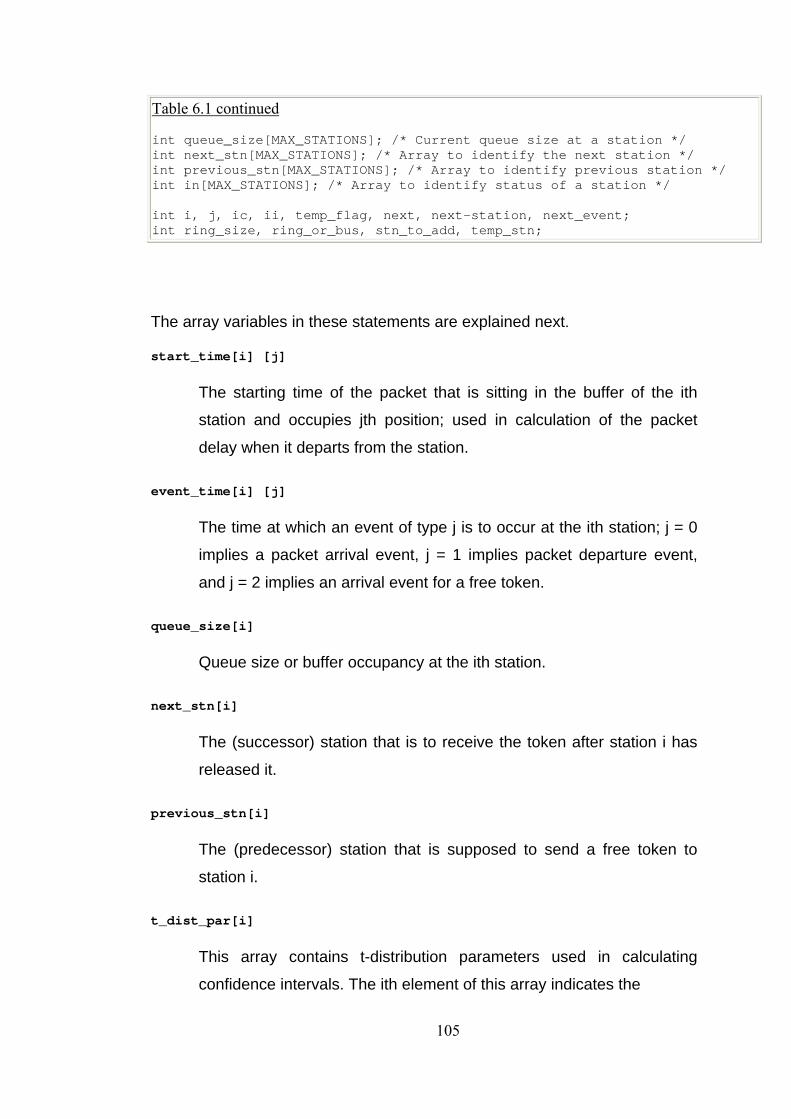
Table 6.1 continued int queue_size[MAX_STATIONS]; /* Current queue size at a station */ int next_stn[MAX_STATIONS]; /* Array to identify the next station */ int previous_stn[MAX_STATIONS]; /* Array to identify previous station */ int in[MAX_STATIONS]; /* Array to identify status of a station */ int i, j, ic, ii, temp_flag, next, next-station, next_event; int ring_size, ring_or_bus, stn_to_add, temp_stn;
The array variables in these statements are explained next.
start_time[i] [j]
The starting time of the packet that is sitting in the buffer of the ith
station and occupies jth position; used in calculation of the packet
delay when it departs from the station.
event_time[i] [j]
The time at which an event of type j is to occur at the ith station; j = 0
implies a packet arrival event, j = 1 implies packet departure event,
and j = 2 implies an arrival event for a free token.
queue_size[i]
Queue size or buffer occupancy at the ith station.
next_stn[i]
The (successor) station that is to receive the token after station i has
released it.
previous_stn[i]
The (predecessor) station that is supposed to send a free token to
station i.
t_dist_par[i]
This array contains t-distribution parameters used in calculating
confidence intervals. The ith element of this array indicates the
105
parameters to be used in calculating 95% confidence intervals with i
degrees of freedom.
delay_ci[i]
This array is used to temporarily hold the values of delay from various
simulation runs with the same input parameters. These values are
eventually used in calculating confidence intervals.
in[i]
This array is used only in token-passing bus LANs. It indicates
whether a station is part of logical ring or not. If in[i] is 1, that implies
station i is a part of the logical ring; and if it is 0, that implies station i is
not a part of the logical ring.
The segment in Table 6.2 marks the beginning of the main body of the
program. The segment starts with some output statements. The variable
arrival_rate is initialized to zero and its value is incremented within a for-loop.
Some of the input variables that are assigned one type of units in the
beginning are converted to a more convenient type of units, in this segment.
This is done merely for programming convenience. For example, the values
of PACKET_LENGTH, TOKEN_LENGTH and STN_LATENCY are initially
assigned in bits and are then converted to their equivalent time units (i.e., the
time it takes to transmit that many bits). The corresponding variables in time
units are packet_time, token_time, and stn_latency, respectively. The
variable tau represents the end-to-end propagation delay, and its value is
calculated assuming that the wave propagation speed on the transmission
medium is 5 microseconds per kilometer. The variable rand-size represents
the largest integer value that the program can handle. This depends on the
computer being used. Thus, in order to have the flexibility of running the
simulation program on any computer, the program uses sizeof(int) function of
the turbo C language to determine the size of the integer in bytes. That
information is used to determine the value of the variable rand_size, which is
then used in random number generation.
106
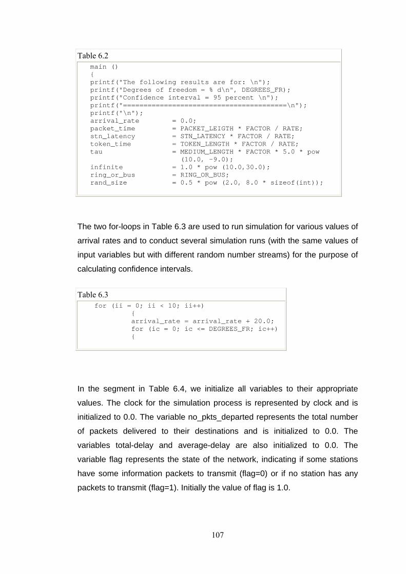
Table 6.2 main () { printf("The following results are for: \n"); printf("Degrees of freedom = % d\n", DEGREES_FR); printf("Confidence interval = 95 percent \n"); printf("========================================\n"); printf("\n"); arrival_rate = 0.0; packet_time = PACKET_LEIGTH * FACTOR / RATE; stn_latency = STN_LATENCY * FACTOR / RATE; token_time = TOKEN_LENGTH * FACTOR / RATE; tau = MEDIUM_LENGTH * FACTOR * 5.0 * pow (10.0, -9.0); infinite = 1.0 * pow (10.0,30.0); ring_or_bus = RING_OR_BUS; rand_size = 0.5 * pow (2.0, 8.0 * sizeof(int));
The two for-loops in Table 6.3 are used to run simulation for various values of
arrival rates and to conduct several simulation runs (with the same values of
input variables but with different random number streams) for the purpose of
calculating confidence intervals.
Table 6.3 for (ii = 0; ii < 10; ii++) { arrival_rate = arrival_rate + 20.0; for (ic = 0; ic <= DEGREES_FR; ic++) {
In the segment in Table 6.4, we initialize all variables to their appropriate
values. The clock for the simulation process is represented by clock and is
initialized to 0.0. The variable no_pkts_departed represents the total number
of packets delivered to their destinations and is initialized to 0.0. The
variables total-delay and average-delay are also initialized to 0.0. The
variable flag represents the state of the network, indicating if some stations
have some information packets to transmit (flag=0) or if no station has any
packets to transmit (flag=1). Initially the value of flag is 1.0.
107
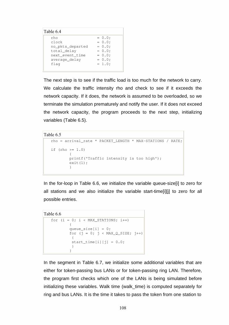
Table 6.4 rho = 0.0; clock = 0.0; no_pkts_departed = 0.0; total_delay = 0.0; next_event_time = 0.0; average_delay = 0.0; flag = 1.0;
The next step is to see if the traffic load is too much for the network to carry.
We calculate the traffic intensity rho and check to see if it exceeds the
network capacity. If it does, the network is assumed to be overloaded, so we
terminate the simulation prematurely and notify the user. If it does not exceed
the network capacity, the program proceeds to the next step, initializing
variables (Table 6.5).
Table 6.5 rho = arrival_rate * PACKET_LENGTH * MAX-STATIONS / RATE; if (rho >= 1.0) { printf("Traffic intensity is too high"); exit(1); }
In the for-loop in Table 6.6, we initialize the variable queue-size[i] to zero for
all stations and we also initialize the variable start-time[i][j] to zero for all
possible entries.
Table 6.6 for (i = 0; i < MAX_STATIONS; i++) { queue_size[i] = 0; for (j = 0; j < MAX_Q_SIZE; j++) { start_time[i][j] = 0.0; } }
In the segment in Table 6.7, we initialize some additional variables that are
either for token-passing bus LANs or for token-passing ring LAN. Therefore,
the program first checks which one of the LANs is being simulated before
initializing these variables. Walk time (walk_time) is computed separately for
ring and bus LANs. It is the time it takes to pass the token from one station to
108
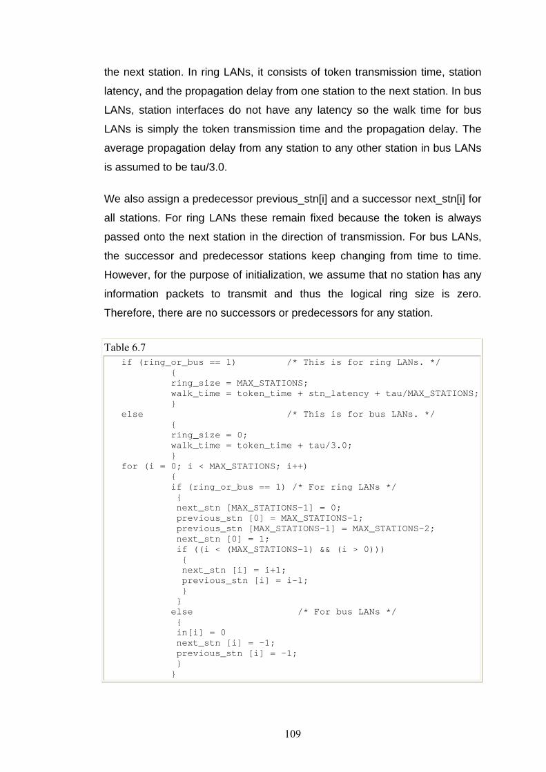
the next station. In ring LANs, it consists of token transmission time, station
latency, and the propagation delay from one station to the next station. In bus
LANs, station interfaces do not have any latency so the walk time for bus
LANs is simply the token transmission time and the propagation delay. The
average propagation delay from any station to any other station in bus LANs
is assumed to be tau/3.0.
We also assign a predecessor previous_stn[i] and a successor next_stn[i] for
all stations. For ring LANs these remain fixed because the token is always
passed onto the next station in the direction of transmission. For bus LANs,
the successor and predecessor stations keep changing from time to time.
However, for the purpose of initialization, we assume that no station has any
information packets to transmit and thus the logical ring size is zero.
Therefore, there are no successors or predecessors for any station.
Table 6.7 if (ring_or_bus == 1) /* This is for ring LANs. */ { ring_size = MAX_STATIONS; walk_time = token_time + stn_latency + tau/MAX_STATIONS; } else /* This is for bus LANs. */ { ring_size = 0; walk_time = token_time + tau/3.0; } for (i = 0; i < MAX_STATIONS; i++) { if (ring_or_bus == 1) /* For ring LANs */ { next_stn [MAX_STATIONS-1] = 0; previous_stn [0] = MAX_STATIONS-1; previous_stn [MAX_STATIONS-1] = MAX_STATIONS-2; next_stn [0] = 1; if ((i < (MAX_STATIONS-1) && (i > 0))) { next_stn [i] = i+1; previous_stn [i] = i-1; } } else /* For bus LANs */ { in[i] = 0 next_stn [i] = -1; previous_stn [i] = -1; } }
109
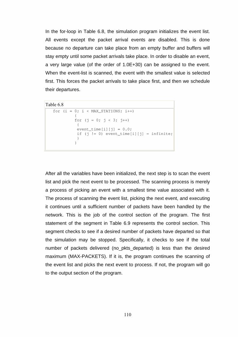
In the for-loop in Table 6.8, the simulation program initializes the event list.
All events except the packet arrival events are disabled. This is done
because no departure can take place from an empty buffer and buffers will
stay empty until some packet arrivals take place. In order to disable an event,
a very large value (of the order of 1.0E+30) can be assigned to the event.
When the event-list is scanned, the event with the smallest value is selected
first. This forces the packet arrivals to take place first, and then we schedule
their departures.
Table 6.8 for (i = 0; i < MAX_STATIONS; i++) { for (j = 0; j < 3; j++) { event_time[i][j] = 0.0; if (j != 0) event_time[i][j] = infinite; } }
After all the variables have been initialized, the next step is to scan the event
list and pick the next event to be processed. The scanning process is merely
a process of picking an event with a smallest time value associated with it.
The process of scanning the event list, picking the next event, and executing
it continues until a sufficient number of packets have been handled by the
network. This is the job of the control section of the program. The first
statement of the segment in Table 6.9 represents the control section. This
segment checks to see if a desired number of packets have departed so that
the simulation may be stopped. Specifically, it checks to see if the total
number of packets delivered (no_pkts_departed) is less than the desired
maximum (MAX-PACKETS). If it is, the program continues the scanning of
the event list and picks the next event to process. If not, the program will go
to the output section of the program.
110
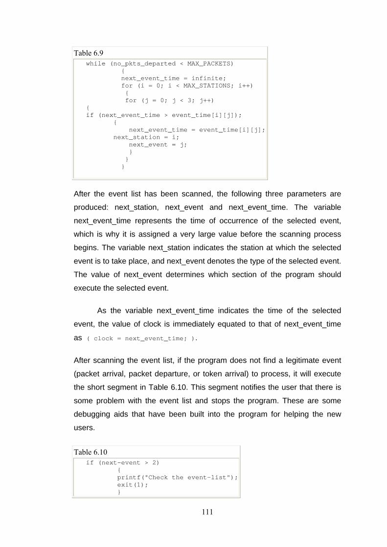
Table 6.9 while (no_pkts_departed < MAX_PACKETS) { next_event_time = infinite; for (i = 0; i < MAX_STATIONS; i++) { for (j = 0; j < 3; j++) { if (next_event_time > event_time[i][j]); { next_event_time = event_time[i][j]; next_station = i; next_event = j; } } }
After the event list has been scanned, the following three parameters are
produced: next_station, next_event and next_event_time. The variable
next_event_time represents the time of occurrence of the selected event,
which is why it is assigned a very large value before the scanning process
begins. The variable next_station indicates the station at which the selected
event is to take place, and next_event denotes the type of the selected event.
The value of next_event determines which section of the program should
execute the selected event.
As the variable next_event_time indicates the time of the selected
event, the value of clock is immediately equated to that of next_event_time
as ( clock = next_event_time; ).
After scanning the event list, if the program does not find a legitimate event
(packet arrival, packet departure, or token arrival) to process, it will execute
the short segment in Table 6.10. This segment notifies the user that there is
some problem with the event list and stops the program. These are some
debugging aids that have been built into the program for helping the new
users.
Table 6.10 if (next-event > 2) { printf("Check the event-list"); exit(1); }
111
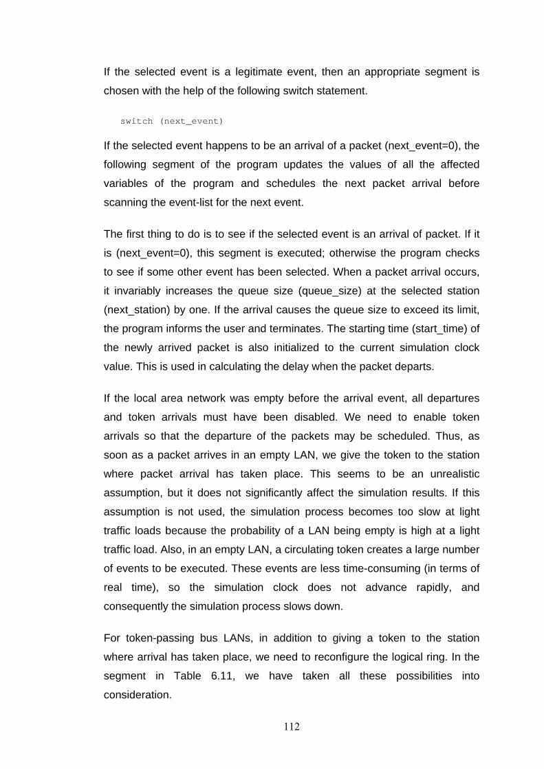
If the selected event is a legitimate event, then an appropriate segment is
chosen with the help of the following switch statement.
switch (next_event)
If the selected event happens to be an arrival of a packet (next_event=0), the
following segment of the program updates the values of all the affected
variables of the program and schedules the next packet arrival before
scanning the event-list for the next event.
The first thing to do is to see if the selected event is an arrival of packet. If it
is (next_event=0), this segment is executed; otherwise the program checks
to see if some other event has been selected. When a packet arrival occurs,
it invariably increases the queue size (queue_size) at the selected station
(next_station) by one. If the arrival causes the queue size to exceed its limit,
the program informs the user and terminates. The starting time (start_time) of
the newly arrived packet is also initialized to the current simulation clock
value. This is used in calculating the delay when the packet departs.
If the local area network was empty before the arrival event, all departures
and token arrivals must have been disabled. We need to enable token
arrivals so that the departure of the packets may be scheduled. Thus, as
soon as a packet arrives in an empty LAN, we give the token to the station
where packet arrival has taken place. This seems to be an unrealistic
assumption, but it does not significantly affect the simulation results. If this
assumption is not used, the simulation process becomes too slow at light
traffic loads because the probability of a LAN being empty is high at a light
traffic load. Also, in an empty LAN, a circulating token creates a large number
of events to be executed. These events are less time-consuming (in terms of
real time), so the simulation clock does not advance rapidly, and
consequently the simulation process slows down.
For token-passing bus LANs, in addition to giving a token to the station
where arrival has taken place, we need to reconfigure the logical ring. In the
segment in Table 6.11, we have taken all these possibilities into
consideration.
112
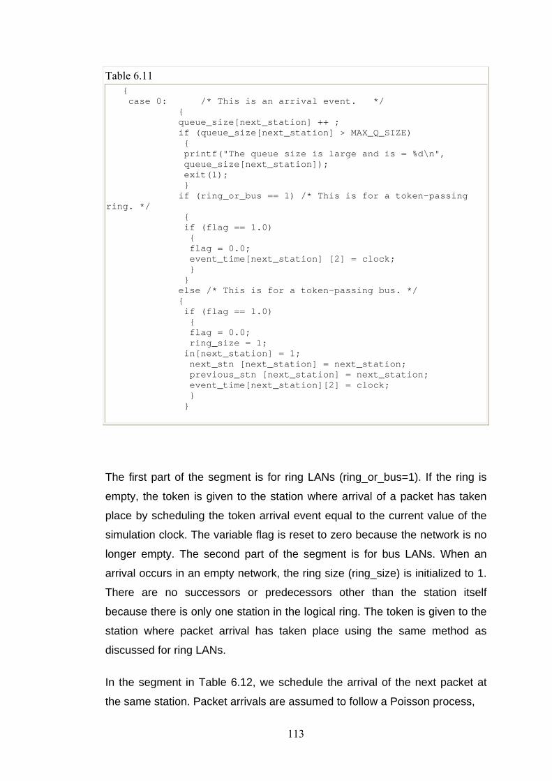
Table 6.11 { case 0: /* This is an arrival event. */ { queue_size[next_station] ++ ; if (queue_size[next_station] > MAX_Q_SIZE) { printf("The queue size is large and is = %d\n", queue_size[next_station]); exit(1); } if (ring_or_bus == 1) /* This is for a token-passing ring. */ { if (flag == 1.0) { flag = 0.0; event_time[next_station] [2] = clock; } } else /* This is for a token-passing bus. */ { if (flag == 1.0) { flag = 0.0; ring_size = 1; in[next_station] = 1; next_stn [next_station] = next_station; previous_stn [next_station] = next_station; event_time[next_station][2] = clock; } }
The first part of the segment is for ring LANs (ring_or_bus=1). If the ring is
empty, the token is given to the station where arrival of a packet has taken
place by scheduling the token arrival event equal to the current value of the
simulation clock. The variable flag is reset to zero because the network is no
longer empty. The second part of the segment is for bus LANs. When an
arrival occurs in an empty network, the ring size (ring_size) is initialized to 1.
There are no successors or predecessors other than the station itself
because there is only one station in the logical ring. The token is given to the
station where packet arrival has taken place using the same method as
discussed for ring LANs.
In the segment in Table 6.12, we schedule the arrival of the next packet at
the same station. Packet arrivals are assumed to follow a Poisson process,
113
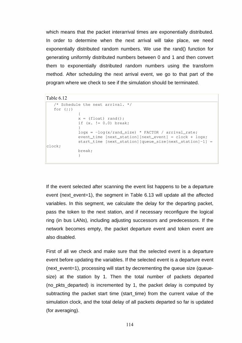
which means that the packet interarrival times are exponentially distributed.
In order to determine when the next arrival will take place, we need
exponentially distributed random numbers. We use the rand() function for
generating uniformly distributed numbers between 0 and 1 and then convert
them to exponentially distributed random numbers using the transform
method. After scheduling the next arrival event, we go to that part of the
program where we check to see if the simulation should be terminated.
Table 6.12 /* Schedule the next arrival. */ for (;;) { x = (float) rand(); if (x. != 0.0) break; } logx = -log(x/rand_size) * FACTOR / arrival_rate; event_time [next_station][next_event] = clock + logx; start_time [next_station][queue_size[next_station]-1] = clock; break; }
If the event selected after scanning the event list happens to be a departure
event (next_event=1), the segment in Table 6.13 will update all the affected
variables. In this segment, we calculate the delay for the departing packet,
pass the token to the next station, and if necessary reconfigure the logical
ring (in bus LANs), including adjusting successors and predecessors. If the
network becomes empty, the packet departure event and token event are
also disabled.
First of all we check and make sure that the selected event is a departure
event before updating the variables. If the selected event is a departure event
(next_event=1), processing will start by decrementing the queue size (queue-
size) at the station by 1. Then the total number of packets departed
(no_pkts_departed) is incremented by 1, the packet delay is computed by
subtracting the packet start time (start_time) from the current value of the
simulation clock, and the total delay of all packets departed so far is updated
(for averaging).
114
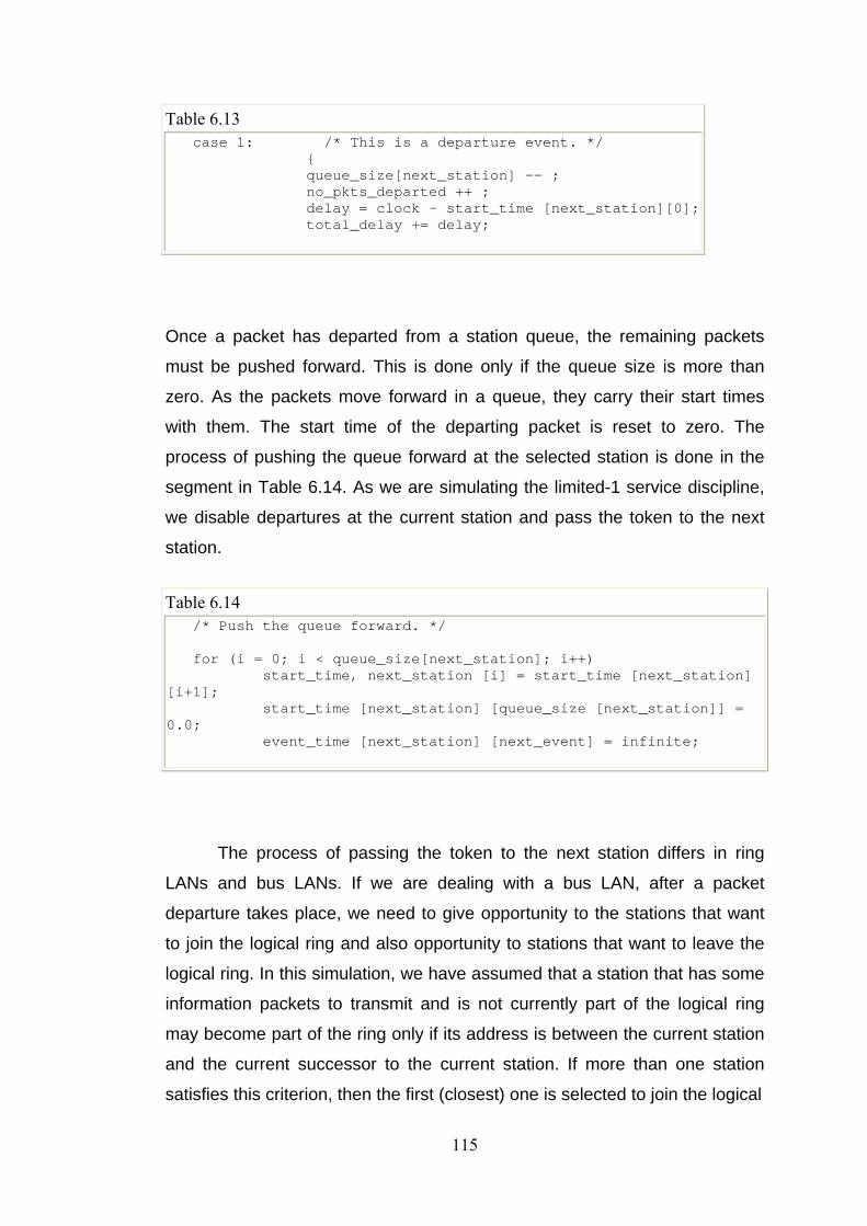
Table 6.13 case 1: /* This is a departure event. */ { queue_size[next_station] -- ; no_pkts_departed ++ ; delay = clock - start_time [next_station][0]; total_delay += delay;
Once a packet has departed from a station queue, the remaining packets
must be pushed forward. This is done only if the queue size is more than
zero. As the packets move forward in a queue, they carry their start times
with them. The start time of the departing packet is reset to zero. The
process of pushing the queue forward at the selected station is done in the
segment in Table 6.14. As we are simulating the limited-1 service discipline,
we disable departures at the current station and pass the token to the next
station.
Table 6.14 /* Push the queue forward. */ for (i = 0; i < queue_size[next_station]; i++) start_time, next_station [i] = start_time [next_station] [i+1]; start_time [next_station] [queue_size [next_station]] = 0.0; event_time [next_station] [next_event] = infinite;
The process of passing the token to the next station differs in ring
LANs and bus LANs. If we are dealing with a bus LAN, after a packet
departure takes place, we need to give opportunity to the stations that want
to join the logical ring and also opportunity to stations that want to leave the
logical ring. In this simulation, we have assumed that a station that has some
information packets to transmit and is not currently part of the logical ring
may become part of the ring only if its address is between the current station
and the current successor to the current station. If more than one station
satisfies this criterion, then the first (closest) one is selected to join the logical
115
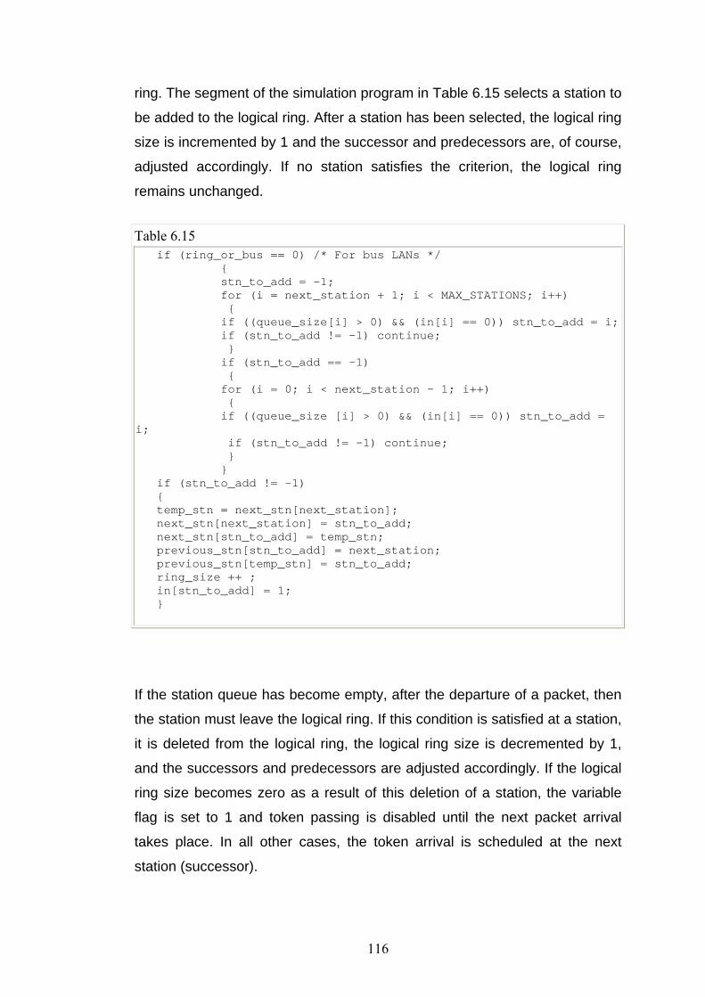
ring. The segment of the simulation program in Table 6.15 selects a station to
be added to the logical ring. After a station has been selected, the logical ring
size is incremented by 1 and the successor and predecessors are, of course,
adjusted accordingly. If no station satisfies the criterion, the logical ring
remains unchanged.
Table 6.15 if (ring_or_bus == 0) /* For bus LANs */ { stn_to_add = -1; for (i = next_station + 1; i < MAX_STATIONS; i++) { if ((queue_size[i] > 0) && (in[i] == 0)) stn_to_add = i; if (stn_to_add != -1) continue; } if (stn_to_add == -1) { for (i = 0; i < next_station - 1; i++) { if ((queue_size [i] > 0) && (in[i] == 0)) stn_to_add = i; if (stn_to_add != -1) continue; } } if (stn_to_add != -1) { temp_stn = next_stn[next_station]; next_stn[next_station] = stn_to_add; next_stn[stn_to_add] = temp_stn; previous_stn[stn_to_add] = next_station; previous_stn[temp_stn] = stn_to_add; ring_size ++ ; in[stn_to_add] = 1; }
If the station queue has become empty, after the departure of a packet, then
the station must leave the logical ring. If this condition is satisfied at a station,
it is deleted from the logical ring, the logical ring size is decremented by 1,
and the successors and predecessors are adjusted accordingly. If the logical
ring size becomes zero as a result of this deletion of a station, the variable
flag is set to 1 and token passing is disabled until the next packet arrival
takes place. In all other cases, the token arrival is scheduled at the next
station (successor).
116
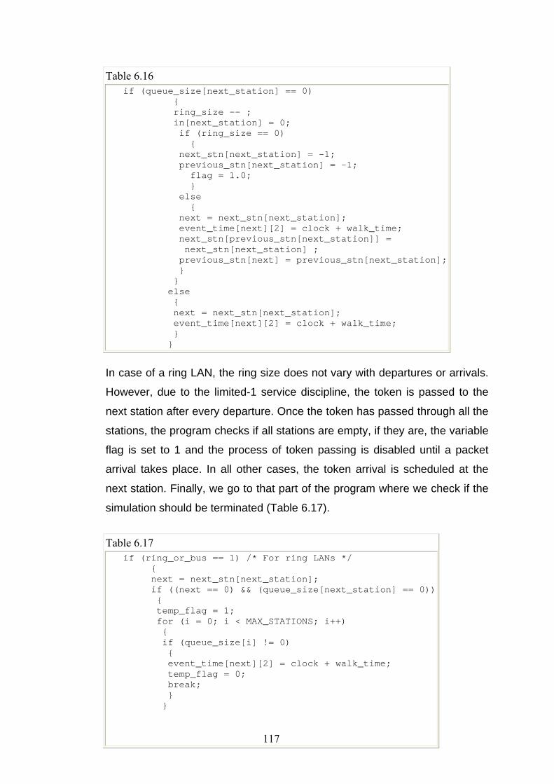
Table 6.16 if (queue_size[next_station] == 0) { ring_size -- ; in[next_station] = 0; if (ring_size == 0) { next_stn[next_station] = -1; previous_stn[next_station] = -1; flag = 1.0; } else { next = next_stn[next_station]; event_time[next][2] = clock + walk_time; next_stn[previous_stn[next_station]] = next_stn[next_station] ; previous_stn[next] = previous_stn[next_station]; } } else { next = next_stn[next_station]; event_time[next][2] = clock + walk_time; } }
In case of a ring LAN, the ring size does not vary with departures or arrivals.
However, due to the limited-1 service discipline, the token is passed to the
next station after every departure. Once the token has passed through all the
stations, the program checks if all stations are empty, if they are, the variable
flag is set to 1 and the process of token passing is disabled until a packet
arrival takes place. In all other cases, the token arrival is scheduled at the
next station. Finally, we go to that part of the program where we check if the
simulation should be terminated (Table 6.17).
Table 6.17 if (ring_or_bus == 1) /* For ring LANs */ { next = next_stn[next_station]; if ((next == 0) && (queue_size[next_station] == 0)) { temp_flag = 1; for (i = 0; i < MAX_STATIONS; i++) { if (queue_size[i] != 0) { event_time[next][2] = clock + walk_time; temp_flag = 0; break; } }
117
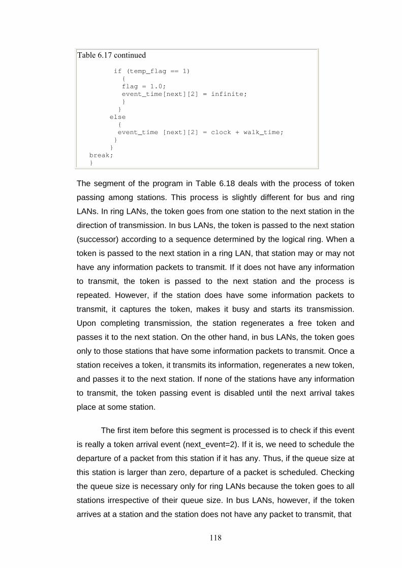
Table 6.17 continued if (temp_flag == 1) { flag = 1.0; event_time[next][2] = infinite; } } else { event_time [next][2] = clock + walk_time; } } break; }
The segment of the program in Table 6.18 deals with the process of token
passing among stations. This process is slightly different for bus and ring
LANs. In ring LANs, the token goes from one station to the next station in the
direction of transmission. In bus LANs, the token is passed to the next station
(successor) according to a sequence determined by the logical ring. When a
token is passed to the next station in a ring LAN, that station may or may not
have any information packets to transmit. If it does not have any information
to transmit, the token is passed to the next station and the process is
repeated. However, if the station does have some information packets to
transmit, it captures the token, makes it busy and starts its transmission.
Upon completing transmission, the station regenerates a free token and
passes it to the next station. On the other hand, in bus LANs, the token goes
only to those stations that have some information packets to transmit. Once a
station receives a token, it transmits its information, regenerates a new token,
and passes it to the next station. If none of the stations have any information
to transmit, the token passing event is disabled until the next arrival takes
place at some station.
The first item before this segment is processed is to check if this event
is really a token arrival event (next_event=2). If it is, we need to schedule the
departure of a packet from this station if it has any. Thus, if the queue size at
this station is larger than zero, departure of a packet is scheduled. Checking
the queue size is necessary only for ring LANs because the token goes to all
stations irrespective of their queue size. In bus LANs, however, if the token
arrives at a station and the station does not have any packet to transmit, that
118
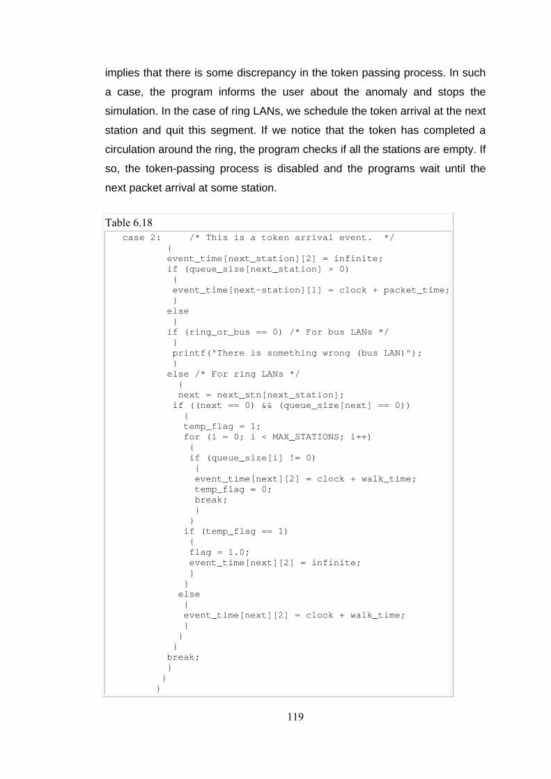
implies that there is some discrepancy in the token passing process. In such
a case, the program informs the user about the anomaly and stops the
simulation. In the case of ring LANs, we schedule the token arrival at the next
station and quit this segment. If we notice that the token has completed a
circulation around the ring, the program checks if all the stations are empty. If
so, the token-passing process is disabled and the programs wait until the
next packet arrival at some station.
Table 6.18 case 2: /* This is a token arrival event. */ { event_time[next_station][2] = infinite; if (queue_size[next_station] > 0) { event_time[next-station][1] = clock + packet_time; } else } if (ring_or_bus == 0) /* For bus LANs */ } printf("There is something wrong (bus LAN)"); } else /* For ring LANs */ { next = next_stn[next_station]; if ((next == 0) && (queue_size[next] == 0)) { temp_flag = 1; for (i = 0; i < MAX_STATIONS; i++) { if (queue_size[i] != 0) { event_time[next][2] = clock + walk_time; temp_flag = 0; break; } } if (temp_flag == 1) { flag = 1.0; event_time[next][2] = infinite; } } else { event_time[next][2] = clock + walk_time; } } } break; } } }
119
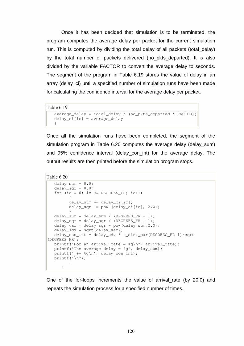
Once it has been decided that simulation is to be terminated, the
program computes the average delay per packet for the current simulation
run. This is computed by dividing the total delay of all packets (total_delay)
by the total number of packets delivered (no_pkts_departed). It is also
divided by the variable FACTOR to convert the average delay to seconds.
The segment of the program in Table 6.19 stores the value of delay in an
array (delay_ci) until a specified number of simulation runs have been made
for calculating the confidence interval for the average delay per packet.
Table 6.19 average_delay = total_delay / (no_pkts_departed * FACTOR); delay_ci[ic] = average_delay }
Once all the simulation runs have been completed, the segment of the
simulation program in Table 6.20 computes the average delay (delay_sum)
and 95% confidence interval (delay_con_int) for the average delay. The
output results are then printed before the simulation program stops.
Table 6.20 delay_sum = 0.0; delay_sqr = 0.0; for (ic = 0; ic <= DEGREES_FR; ic++) { delay_sum += delay_ci[ic]; delay_sqr += pow (delay_ci[ic], 2.0); } delay_sum = delay_sum / (DEGREES_FR + 1); delay_sqr = delay_sqr / (DEGREES_FR + 1); delay_var = delay_sqr - pow(delay_sum,2.0); delay_sdv = sqrt(delay_var); delay_con_int = delay_sdv * t_dist_par[DEGREES_FR-1]/sqrt (DEGREES_FR); printf("For an arrival rate = %g\n", arrival_rate); printf("The average delay = %g", delay_sum); printf(" +- %g\n", delay_con_int); printf("\n"); } }
One of the for-loops increments the value of arrival_rate (by 20.0) and
repeats the simulation process for a specified number of times.
120
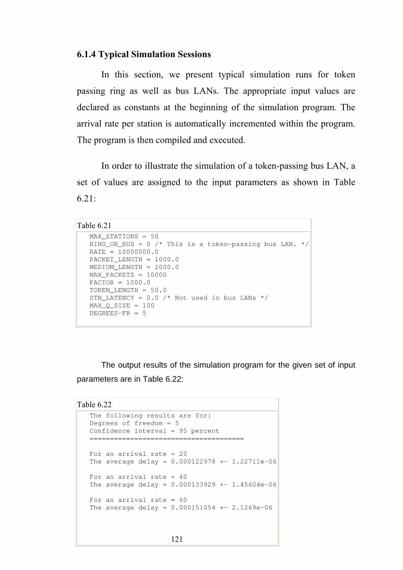
6.1.4 Typical Simulation Sessions
In this section, we present typical simulation runs for token
passing ring as well as bus LANs. The appropriate input values are
declared as constants at the beginning of the simulation program. The
arrival rate per station is automatically incremented within the program.
The program is then compiled and executed.
In order to illustrate the simulation of a token-passing bus LAN, a
set of values are assigned to the input parameters as shown in Table
6.21:
Table 6.21 MAX_STATIONS = 50 RING_OR_BUS = 0 /* This is a token-passing bus LAN. */ RATE = 10000000.0 PACKET_LENGTH = 1000.0 MEDIUM_LENGTH = 2000.0 MAX_PACKETS = 10000 FACTOR = 1000.0 TOKEN_LENGTH = 50.0 STN_LATENCY = 0.0 /* Not used in bus LANs */ MAX_Q_SIZE = 100 DEGREES-FR = 5
The output results of the simulation program for the given set of input
parameters are in Table 6.22:
Table 6.22 The following results are for: Degrees of freedom = 5 Confidence interval = 95 percent ====================================== For an arrival rate = 20 The average delay = 0.000122978 +- 1.22711e-06 For an arrival rate = 40 The average delay = 0.000133929 +- 1.45604e-06 For an arrival rate = 60 The average delay = 0.000151054 +- 2.1269e-06
121
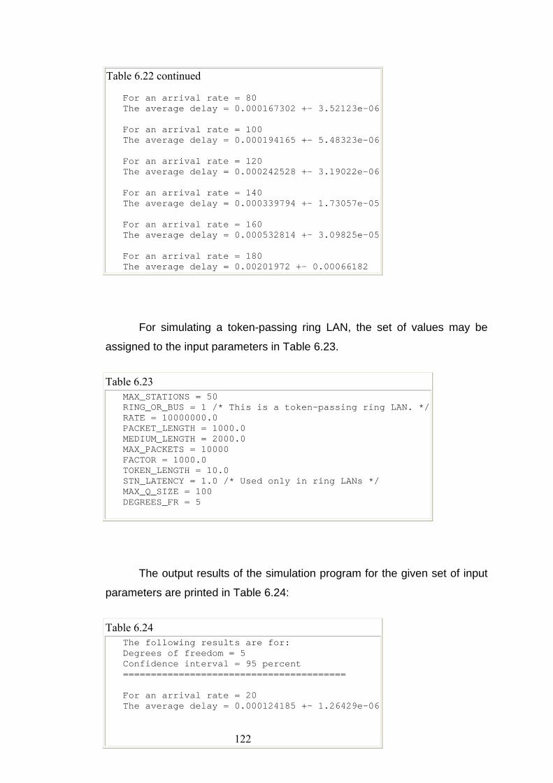
Table 6.22 continued For an arrival rate = 80 The average delay = 0.000167302 +- 3.52123e-06 For an arrival rate = 100 The average delay = 0.000194165 +- 5.48323e-06 For an arrival rate = 120 The average delay = 0.000242528 +- 3.19022e-06 For an arrival rate = 140 The average delay = 0.000339794 +- 1.73057e-05 For an arrival rate = 160 The average delay = 0.000532814 +- 3.09825e-05 For an arrival rate = 180 The average delay = 0.00201972 +- 0.00066182
For simulating a token-passing ring LAN, the set of values may be
assigned to the input parameters in Table 6.23.
Table 6.23 MAX_STATIONS = 50 RING_OR_BUS = 1 /* This is a token-passing ring LAN. */ RATE = 10000000.0 PACKET_LENGTH = 1000.0 MEDIUM_LENGTH = 2000.0 MAX_PACKETS = 10000 FACTOR = 1000.0 TOKEN_LENGTH = 10.0 STN_LATENCY = 1.0 /* Used only in ring LANs */ MAX_Q_SIZE = 100 DEGREES_FR = 5
The output results of the simulation program for the given set of input
parameters are printed in Table 6.24:
Table 6.24 The following results are for: Degrees of freedom = 5 Confidence interval = 95 percent ======================================== For an arrival rate = 20 The average delay = 0.000124185 +- 1.26429e-06
122
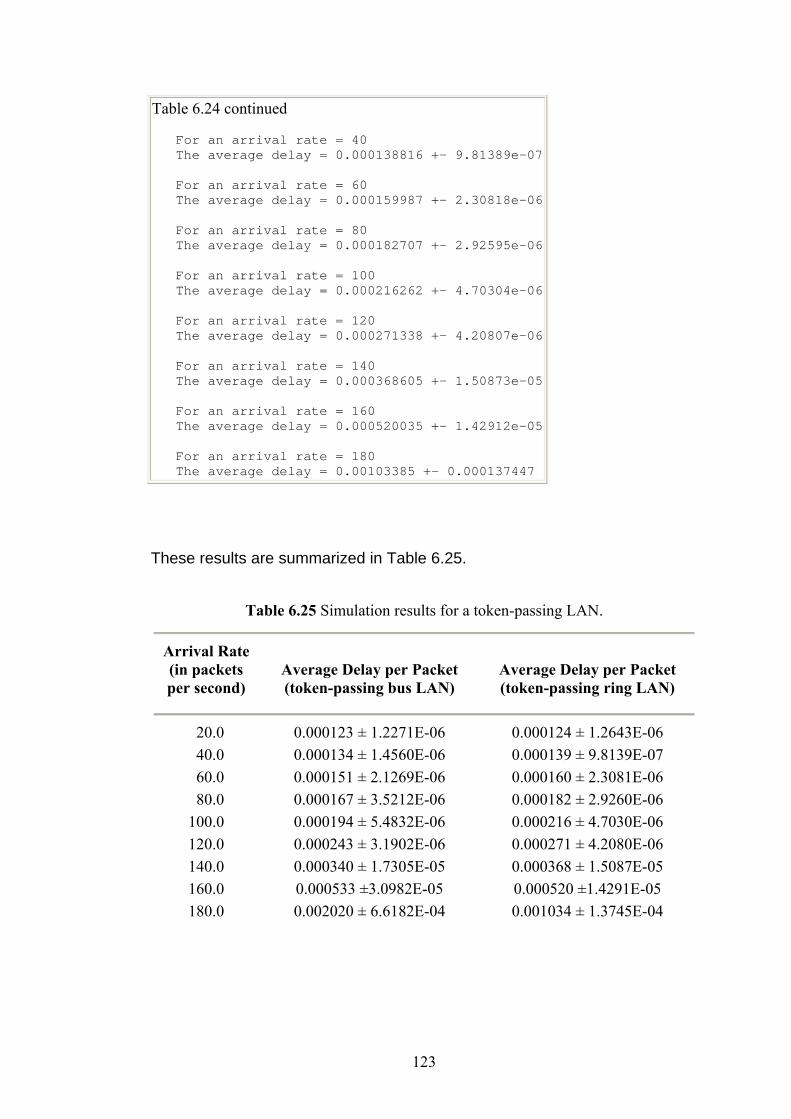
Table 6.24 continued For an arrival rate = 40 The average delay = 0.000138816 +- 9.81389e-07 For an arrival rate = 60 The average delay = 0.000159987 +- 2.30818e-06 For an arrival rate = 80 The average delay = 0.000182707 +- 2.92595e-06 For an arrival rate = 100 The average delay = 0.000216262 +- 4.70304e-06 For an arrival rate = 120 The average delay = 0.000271338 +- 4.20807e-06 For an arrival rate = 140 The average delay = 0.000368605 +- 1.50873e-05 For an arrival rate = 160 The average delay = 0.000520035 +- 1.42912e-05 For an arrival rate = 180 The average delay = 0.00103385 +- 0.000137447
These results are summarized in Table 6.25.
Table 6.25 Simulation results for a token-passing LAN.
Arrival Rate (in packets per second)
Average Delay per Packet (token-passing bus LAN)
Average Delay per Packet (token-passing ring LAN)
20.0 0.000123 ± 1.2271E-06 0.000124 ± 1.2643E-06 40.0 0.000134 ± 1.4560E-06 0.000139 ± 9.8139E-07 60.0 0.000151 ± 2.1269E-06 0.000160 ± 2.3081E-06 80.0 0.000167 ± 3.5212E-06 0.000182 ± 2.9260E-06 100.0 0.000194 ± 5.4832E-06 0.000216 ± 4.7030E-06 120.0 0.000243 ± 3.1902E-06 0.000271 ± 4.2080E-06 140.0 0.000340 ± 1.7305E-05 0.000368 ± 1.5087E-05 160.0 0.000533 ±3.0982E-05 0.000520 ±1.4291E-05 180.0 0.002020 ± 6.6182E-04 0.001034 ± 1.3745E-04
123

Chapter Seven
Conclusion and Recommendations for future work
Chapter Seven Conclusion and Recommendations for future work
7.1 Conclusion:
The objective of the research disclosed in this thesis was to study
the factors that affect local area network performance, since the most
important issue in the networking is how to achieve maximum
performance, so this project has present the key principle and goals of
network performance study.
The frame rate in the Ethernet network was calculated according
to the frame lengths first mathematically and by using a BASIC language
program and then the information transfer rate was computed, and was
found that as large as frame length more information transfer rate
occurred.
A model was developed to represent the flow of data on token ring
networks, and then the model was exercised both manually as well as
through the use of a BASIC language program, and found that the frame
rate depends on the number of stations on the network and the ring
length as well as the frame length.
Finally C-programs were designed to simulate the CSMA/CD and
Token-passing networks. The simulation programs were described in
detail, from providing input parameters to printing output results. The
output results are presented in terms of the average delay per packet, the
average throughput, the average utilization, and the average collision
rate. The results are presented with 95% confidence intervals.
124
7.2 Recommendations for future work:
Additional work is still needed in the area of factors affecting
LAN performance. Especially, factors were not calculated in this project
like Jitter and error rate.
Also we can make new programs or modify these simulation
programs to obtain the delay distribution.
125
References:
[1] IEEE Standards for Local and metropolitan area networks, std 802,2002.
[2] William Stallings, "Local and Metropolitan Area Networks" Fifth Edition.
[3] Gilbert Held, "Enhancing LAN Performance" Fourth Edition, Auerbach Publications, 2004.
[4] Gilbert Held, "LAN Performance Issues and Answers" Second Edition.
[5] Andrew S. Tanenbaum, "Computer Networks" Fourth Edition, Prentice Hall, 2003.
[6] Dr. K. V. Prasad, "Principles of Digital Communication Systems and Computer Networks" First Edition, CHARLES RIVER MEDIA, 2004.
[7] William Stalling, "Data and Computer Communications" Fifth Edition, Prentice Hall, 1997.
[8] www.erg.abdn.ac.uk/users/gorry/course/lan-pages/csma-cd.html, 1st November 2008.
126

Appendices
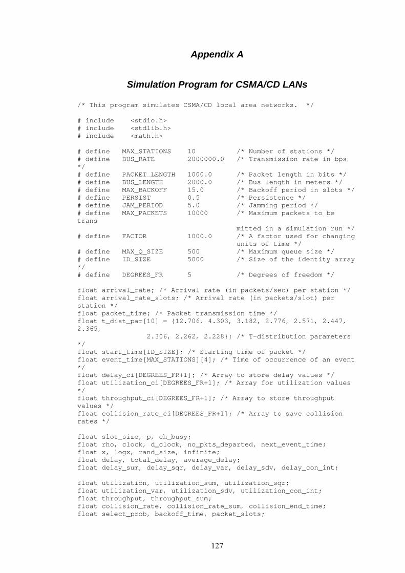
Appendix A
Simulation Program for CSMA/CD LANs
/* This program simulates CSMA/CD local area networks. */ # include <stdio.h> # include <stdlib.h> # include <math.h> # define MAX_STATIONS 10 /* Number of stations */ # define BUS_RATE 2000000.0 /* Transmission rate in bps */ # define PACKET_LENGTH 1000.0 /* Packet length in bits */ # define BUS_LENGTH 2000.0 /* Bus length in meters */ # define MAX_BACKOFF 15.0 /* Backoff period in slots */ # define PERSIST 0.5 /* Persistence */ # define JAM_PERIOD 5.0 /* Jamming period */ # define MAX_PACKETS 10000 /* Maximum packets to be trans mitted in a simulation run */ # define FACTOR 1000.0 /* A factor used for changing units of time */ # define MAX_Q_SIZE 500 /* Maximum queue size */ # define ID_SIZE 5000 /* Size of the identity array */ # define DEGREES_FR 5 /* Degrees of freedom */ float arrival_rate; /* Arrival rate (in packets/sec) per station */ float arrival_rate_slots; /* Arrival rate (in packets/slot) per station */ float packet_time; /* Packet transmission time */ float t_dist_par[10] = {12.706, 4.303, 3.182, 2.776, 2.571, 2.447, 2.365, 2.306, 2.262, 2.228}; /* T-distribution parameters */ float start_time[ID_SIZE]; /* Starting time of packet */ float event_time[MAX_STATIONS][4]; /* Time of occurrence of an event */ float delay_ci[DEGREES_FR+1]; /* Array to store delay values */ float utilization_ci[DEGREES_FR+1]; /* Array for utilization values */ float throughput_ci[DEGREES_FR+1]; /* Array to store throughput values */ float collision_rate_ci[DEGREES_FR+1]; /* Array to save collision rates */ float slot_size, p, ch_busy; float rho, clock, d_clock, no_pkts_departed, next_event_time; float x, logx, rand_size, infinite; float delay, total_delay, average_delay; float delay_sum, delay_sqr, delay_var, delay_sdv, delay_con_int; float utilization, utilization_sum, utilization_sqr; float utilization_var, utilization_sdv, utilization_con_int; float throughput, throughput_sum; float collision_rate, collision_rate_sum, collision_end_time; float select_prob, backoff_time, packet_slots;
127
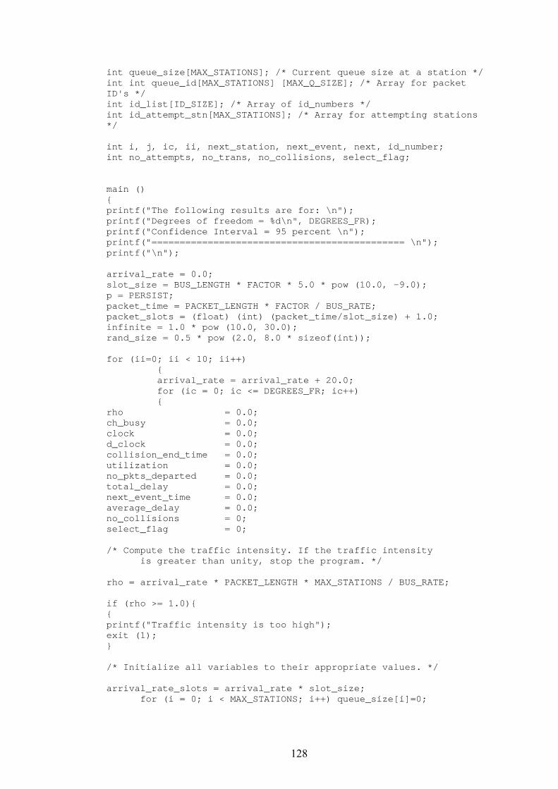
int queue_size[MAX_STATIONS]; /* Current queue size at a station */ int int queue_id[MAX_STATIONS] [MAX_Q_SIZE]; /* Array for packet ID's */ int id_list[ID_SIZE]; /* Array of id_numbers */ int id_attempt_stn[MAX_STATIONS]; /* Array for attempting stations */ int i, j, ic, ii, next_station, next_event, next, id_number; int no_attempts, no_trans, no_collisions, select_flag; main () { printf("The following results are for: \n"); printf("Degrees of freedom = %d\n", DEGREES_FR); printf("Confidence Interval = 95 percent \n"); printf("============================================= \n"); printf("\n"); arrival_rate = 0.0; slot_size = BUS_LENGTH * FACTOR * 5.0 * pow (10.0, -9.0); p = PERSIST; packet_time = PACKET_LENGTH * FACTOR / BUS_RATE; packet_slots = (float) (int) (packet_time/slot_size) + 1.0; infinite = 1.0 * pow (10.0, 30.0); rand_size = 0.5 * pow (2.0, 8.0 * sizeof(int)); for (ii=0; ii < 10; ii++) { arrival_rate = arrival_rate + 20.0; for (ic = 0; ic <= DEGREES_FR; ic++) { rho = 0.0; ch_busy = 0.0; clock = 0.0; d_clock = 0.0; collision_end_time = 0.0; utilization = 0.0; no_pkts_departed = 0.0; total_delay = 0.0; next_event_time = 0.0; average_delay = 0.0; no_collisions = 0; select_flag = 0; /* Compute the traffic intensity. If the traffic intensity is greater than unity, stop the program. */ rho = arrival_rate * PACKET_LENGTH * MAX_STATIONS / BUS_RATE; if (rho >= 1.0){ { printf("Traffic intensity is too high"); exit (1); } /* Initialize all variables to their appropriate values. */ arrival_rate_slots = arrival_rate * slot_size; for (i = 0; i < MAX_STATIONS; i++) queue_size[i]=0;
128
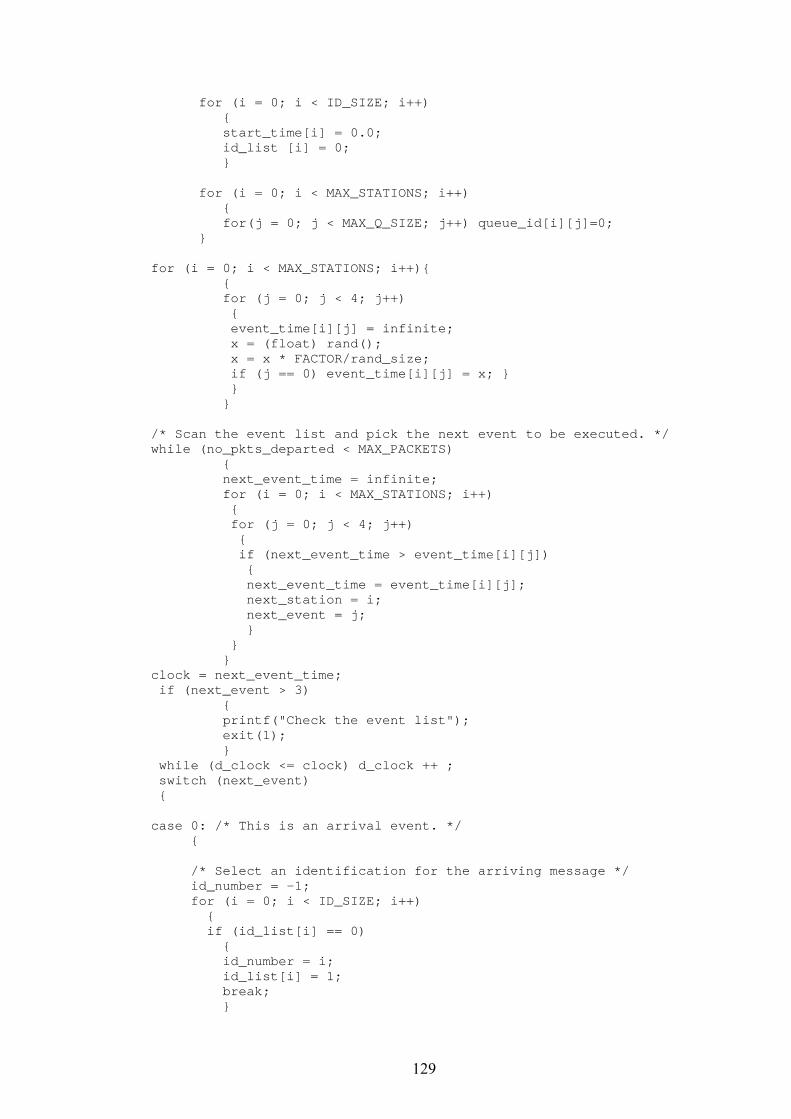
for (i = 0; i < ID_SIZE; i++) { start_time[i] = 0.0; id_list [i] = 0; } for (i = 0; i < MAX_STATIONS; i++) { for(j = 0; j < MAX_Q_SIZE; j++) queue_id[i][j]=0; } for (i = 0; i < MAX_STATIONS; i++){ { for (j = 0; j < 4; j++) { event_time[i][j] = infinite; x = (float) rand(); x = x * FACTOR/rand_size; if (j == 0) event_time[i][j] = x; } } } /* Scan the event list and pick the next event to be executed. */ while (no_pkts_departed < MAX_PACKETS) { next_event_time = infinite; for (i = 0; i < MAX_STATIONS; i++) { for (j = 0; j < 4; j++) { if (next_event_time > event_time[i][j]) { next_event_time = event_time[i][j]; next_station = i; next_event = j; } } } clock = next_event_time; if (next_event > 3) { printf("Check the event list"); exit(1); } while (d_clock <= clock) d_clock ++ ; switch (next_event) { case 0: /* This is an arrival event. */ { /* Select an identification for the arriving message */ id_number = -1; for (i = 0; i < ID_SIZE; i++) { if (id_list[i] == 0) { id_number = i; id_list[i] = 1; break; }
129
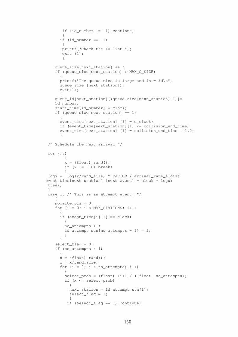
if (id_number != -1) continue; } if (id_number == -1) { printf("Check the ID-list."); exit (1); } queue_size[next_station] ++ ; if (queue_size[next_station] > MAX_Q_SIZE) { printf("The queue size is large and is = %d\n", queue_size [next_station]); exit(1); } queue_id[next_station][(queue-size[next_station]-1)]= 1d_number; start_time[id_number] = clock; if (queue_size[next_station] == 1) { event_time[next_station] [1] = d_clock; if (event_time[next_station][1] <= collision_end_time) event_time[next_station] [1] = collision_end_time + 1.0; } /* Schedule the next arrival */ for (;;) { x = (float) rand(); if (x != 0.0) break; } logx = -log(x/rand_size) * FACTOR / arrival_rate_slots; event_time[next_station] [next_event] = clock + logx; break; } case 1: /* This is an attempt event. */ { no_attempts = 0; for (i = 0; i < MAX_STATIONS; i++) { if (event_time[i][1] == clock) { no_attempts ++; id_attempt_stn[no_attempts - 1] = i; } } select_flag = 0; if (no_attempts > 1) { x = (float) rand(); x = x/rand_size; for (i = 0; i < no_attempts; i++) { select_prob = (float) (i+1)/ ((float) no_attempts); if (x <= select_prob) { next_station = id_attempt_stn[i]; select_flag = 1; } if (select_flag == 1) continue;
130
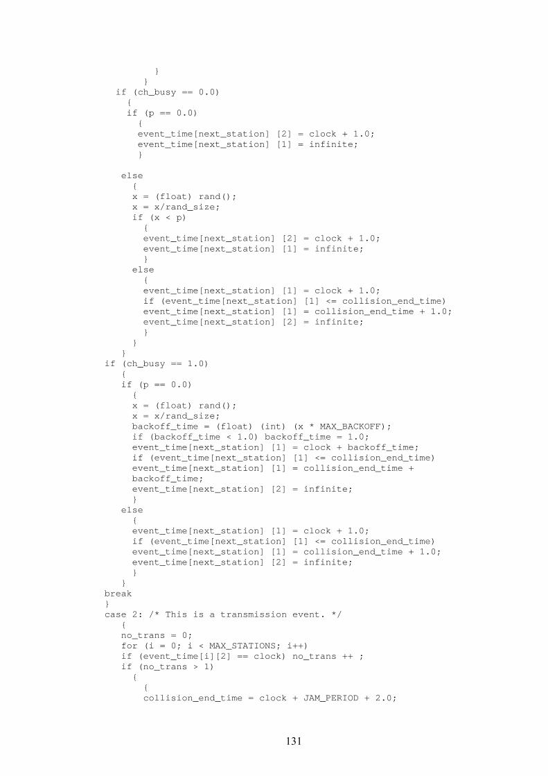
} } if (ch_busy == 0.0) { if (p == 0.0) { event_time[next_station] [2] = clock + 1.0; event_time[next_station] [1] = infinite; } else { x = (float) rand(); x = x/rand_size; if (x < p) { event_time[next_station] [2] = clock + 1.0; event_time[next_station] [1] = infinite; } else { event_time[next_station] [1] = clock + 1.0; if (event_time[next_station] [1] <= collision_end_time) event_time[next_station] [1] = collision_end_time + 1.0; event_time[next_station] [2] = infinite; } } } if (ch_busy == 1.0) { if (p == 0.0) { x = (float) rand(); x = x/rand_size; backoff_time = (float) (int) (x * MAX_BACKOFF); if (backoff_time < 1.0) backoff_time = 1.0; event_time[next_station] [1] = clock + backoff_time; if (event_time[next_station] [1] <= collision_end_time) event_time[next_station] [1] = collision_end_time + backoff_time; event_time[next_station] [2] = infinite; } else { event_time[next_station] [1] = clock + 1.0; if (event_time[next_station] [1] <= collision_end_time) event_time[next_station] [1] = collision_end_time + 1.0; event_time[next_station] [2] = infinite; } } break } case 2: /* This is a transmission event. */ { no_trans = 0; for (i = 0; i < MAX_STATIONS; i++) if (event_time[i][2] == clock) no_trans ++ ; if (no_trans > 1) { { collision_end_time = clock + JAM_PERIOD + 2.0;
131
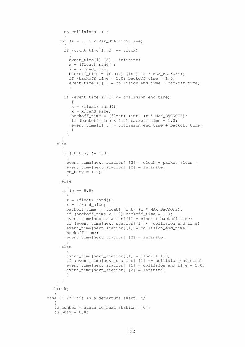
no_collisions ++ ; } for (i = 0; i < MAX_STATIONS; i++) { if (event_time[i][2] == clock) { event_time[i] [2] = infinite; x = (float) rand(); x = x/rand_size; backoff_time = (float) (int) (x * MAX_BACKOFF); if (backoff_time < 1.0) backoff_time = 1.0; event_time[i][1] = collision_end_time + backoff_time; } if (event_time[i][1] <= collision_end_time) { x = (float) rand(); x = x/rand_size; backoff_time = (float) (int) (x * MAX_BACKOFF); if (backoff_time < 1.0) backoff_time = 1.0; event_time[i][1] = collision_end_time + backoff_time; } } } else { if (ch_busy != 1.0) { event_time[next_station] [3] = clock + packet_slots ; event_time[next_station] [2] = infinite; ch_busy = 1.0; } else { if (p == 0.0) { x = (float) rand(); x = x/rand_size; backoff_time = (float) (int) (x * MAX_BACKOFF); if (backoff_time < 1.0) backoff_time = 1.0; event_time[next_station][1] = clock + backoff_time; if (event_time[next_station][1] <= collision_end_time) event_time[next.station][1] = collision_end_time + backoff_time; event_time[next_station] [2] = infinite; } else { event_time[next_station][1] = clock + 1.0; if (event_time[next_station] [1] <= collision_end_time) event_time[next_station] [1] = collision_end_time + 1.0; event_time[next_station] [2] = infinite; } } } break; } case 3: /* This is a departure event. */ { id_number = queue_id[next_station] [0]; ch_busy = 0.0;
132
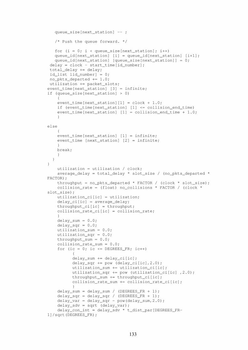
queue_size[next_station] -- ; /* Push the queue forward. */ for (i = 0; i < queue_size[next_station]; i++) queue_id[next_station] [i] = queue_id[next_station] [i+1]; queue_id[next_station] [queue_size[next_station]] = 0; delay = clock - start_time[id_number]; total_delay += delay; id_list lid_number] = 0; no_pkts_departed += 1.0; utilization += packet_slots; event_time[next_station] [3] = infinite; if (queue_size[next_station] > 0) { event_time[next_station][1] = clock + 1.0; if (event_time[next_station] [1] <= collision_end_time) event_time[next_station] [1] = collision_end_time + 1.0; } else { event_time[next_station] [1] = infinite; event_time [next_station] [2] = infinite; } break; } } } utilization = utilization / clock; average_delay = total_delay * slot_size / (no_pkts_departed * FACTOR); throughput = no_pkts_departed * FACTOR / (clock * slot_size); collision_rate = (float) no_collisions * FACTOR / (clock * slot_size); utilization_ci[ic] = utilization; delay_ci[ic] = average_delay; throughput_ci[ic] = throughput; collision_rate_ci[ic] = collision_rate; } delay_sum = 0.0; delay_sqr = 0.0; utilization_sum = 0.0; utilization_sqr = 0.0; throughput_sum = 0.0; collision_rate_sum = 0.0; for (ic = 0; ic <= DEGREES_FR; ic++) { delay_sum += delay_ci[ic]; delay_sqr += pow (delay_ci[ic],2.0); utilization_sum += utilization_ci[ic]; utilization_sqr += pow (utilization_ci[ic] ,2.0); throughput_sum += throughput_ci[ic]; collision_rate_sum += collision_rate_ci[ic]; } delay_sum = delay_sum / (DEGREES_FR + 1); delay_sqr = delay_sqr / (DEGREES_FR + 1); delay_var = delay_sqr - pow(delay_sum,2.0); delay_sdv = sqrt (delay_var); delay_con_int = delay_sdv * t_dist_par[DEGREES_FR-1]/sqrt(DEGREES_FR);
133
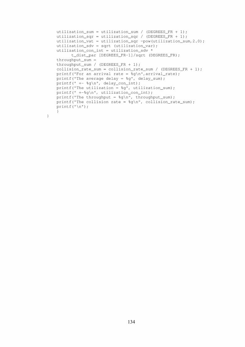
utilization_sum = utilization_sum / (DEGREES_FR + 1); utilization_sqr = utilization_sqr / (DEGREES_FR + 1); utilization_vat = utilization_sqr -pow(utilization_sum,2.0); utilization_sdv = sqrt (utilization_var); utilization_con_int = utilization_sdv * t_dist_par [DEGREES_FR-1]/sqrt (DEGREES_FR); throughput_sum = throughput_sum / (DEGREES_FR + 1); collision_rate_sum = collision_rate_sum / (DEGREES_FR + 1); printf("For an arrival rate = %g\n",arrival_rate); printf("The average delay = %g", delay_sum); printf(" +- %g\n", delay_con_int); printf("The utilization = %g", utilization_sum); printf(" +-%g\n", utilization_con_int); printf("The throughput = %g\n", throughput_sum); printf("The collision rate = %g\n", collision_rate_sum); printf("\n"); } }
134

Appendix B
Simulation for Token-Passing LANs
/* This program simulates token-passing ring and bus LANs. */ # include <stdio.h> # include <stdlib.h> # include <math.h> # define MAX_STATIONS 50 /*Maximum number of stations*/ # define RING_OR_BUS 1 /* Flag to choose ring or bus LAN */ # define RATE 10000000.0 /* Transmission rate in bps */ # define PACKET_LENGTH 1000.0 /* Packet length in bits */ # define NEDIUM_LENGTH 2000.0 /* Medium length in meters */ # define MAX_PACKETS 10000 /* Maximum packets to be transmitted in a simulation run */ # define FACTOR 1000.0 /* A factor used for changing units of time */ # define TOKEN_LENGTH 10.0 /* Token length in bits */ # define STN_LATENCY 1.0 /* Station latency in bits */ # define MAX_Q_SIZE 100 /* Maximum queue size */ # define DEGREES_FR 5 /* Degrees of freedom */ float arrival_rate; /* Arrival rate (in packets/sec) per station */ float packet_time; /* Packet transmission time */ float stn_latency; /* Station latency in time units */ float token_time; /* Token transmission time */ float tau; /* End-to-end propagation delay */ float t_dist_par[10] = {12.706, 4.303, 3.182, 2.776, 2.571, 2.447,2.365, 2.306, 2.262, 2.228}; /* T-distribution parameters */ float start_time[MAX_STATIONS][MAX_Q_SIZE]; /* Starting time of packet */ float event_time[MAX_STATIONS][3]; /* Time of occurrence of an event */ float delay_ci[DEGREES_FR + 1]; /* Array to store delay values */ float rho, clock, no_pkts_departed, next_event_time; float x, logx, flag, infinite, rand_size; float delay, total_delay, average_delay, walk_time; float delay_sum, delay_sqr, delay_var, delay_sdv, delay_con_int; int queue_size[MAX_STATIONS]; /* Current queue size at a station */ int next_stn[MAX_STATIONS]; /* Array to identify the next station */ int previous_stn[MAX_STATIONS]; /* Array to identify previous station */ int in[NAX_STATIONS]; /* Array to identify status of a station */ int i, j, ic, ii, temp_flag, next, next_station, next_event; int ring_size, ring_or_bus, stn_to_add, temp_stn; main () { printf("The following results are for: \n"); printf("Degrees of freedom = % d\n", DEGREES_FR); printf("Confidence interval = 95 percent \n"); printf(" ============================================ \n"); printf("\n"); arrival_rate = 0.0;
135
packet_time = PACKET_LENGTH * FACTOR / RATE; stn_latency = STN_LATENCY * FACTOR / RATE; token_time = TOKEN_LENGTH * FACTOR / RATE; tau = MEDIUM_LENGTH * FACTOR 5.O * pow (10.0, -9.0); infinite = 1.0 * pow (10.0,30.0); ring_or_bus = RING_OR_BUS; rand_size = 0.5 * pot (2.0, 8.0 * sizeof(int)); for (ii = 0; ii < 10; ii++) { arrival_rate = arrival_rate + 20.0; for (ic = 0; ic <= DEGREES_FR; ic++) { rho = 0.0; clock = 0.0; no_pkts_departed = 0.0; tot al_delay = 0.0; next_event_time = 0.0; average_delay = 0.0; flag = 1.0; /* Compute the traffic intensity. If the traffic intensity is greater than unity, stop the program. */ rho = arrival_rate * PACKET_LENGTH * MAX_STATIONS / RATE; if (rho >= 1.0) { printf("Traffic intensity is too high"); exit(1); } /* Initialize all variables to their appropriate values.*/ for (i = 0; i < MAX_STATIONS; i++) { queue_size[i] = 0; for (j = 0; j < MAX_Q_SIZE; j++) { start_time[i][j] = 0.0; } } if (ring_or_bus == 1) /* This is for ring LANs. */ { ring_size = MAX_STATIONS; walk_time token_time + stn_latency + tau/MAX-STATIONS; } else /* This is for bus LANs. */ } ring_size = 0; walk_time = token_time + tau/3.0; } for (i = 0; i < MAX_STATIONS; i++) { if (ring_or_bus == 1) /* For ring LANs */ { next_stn [MAX_STATIONS-1] = 0; previous_stn [0] = MAX_STATIONS-1; previous_stn [MAX_STATIONS-1] = MAX_STATIONS-2; next_stn [0] = 1; if ((i < (MAX_STATIONS-1) && (i > 0))) {
136
next_stn [i] = i+1; previous_stn [i] = i-1; } } else /* For bus LANs */ { in[i] = 0; next_stn [i] = -1; previous_stn [i] = -1; } } for (i = 0; i < MAX_STATIONS; i++) { for (j = 0; j < 3; j++) { event_time[i][j] = 0.0; if (j != 0) event_time[i][j] = infinite; } } /* Scan the event list and pick the next event to be executed. */ while (no_pkts_departed < MAX_PACKETS) { next_event_time = infinite; for (i = 0; i < MAX_STATIONS; i++) { for (j = 0; j < 3; j++) { if (next_event_time > event_time[i][j]) { next_event_time = event_time[i][j]; next_station = i; next_event = j; } } } clock = next_event_time; if (next_event > 2) { printf("Check the event-list"); exit(1); } switch (next_event) { case 0: /* This is an arrival event. */ { queue_size[next_station] ++ ; if (queue_size[next_station] > MAX_Q_SIZE) { printf("The queue size is large and is = %d\n", queue_size[next_station]); exit(1); } if (ring_or_bus == 1) /* This is for a token-passing ring. */ { if (flag == 1.0) { flag = 0.0; event_time[next_station][2] = clock; } }
137
else /* This is for a token-passing bus. */ { if (flag == 1.0) flag = 0.0; ring_size = 1; in[next_station] = 1; next_stn [next_station] = next_station; previous_stn [next_station] = next_station; event_time[next_station][2] = clock; } } /* Schedule the next arrival. */ for (;;) { x = (float) rand(); if (x != 0.0) break; } logx = -log(x/rand_size) * FACTOR / arrival_rate; event_time[next_station][next_event] = clock + logx; start_time [next_station][queue_size[next_station]-1] = clock; break; } case 1: /* This is a departure event. */ { queue_size[next_station] -- ; no_pkts_departed ++ ; delay = clock - start_time [next_station][0]; total_delay += delay; /* Push the queue forward. */ for (i = 0; i < queue_size[next_station]; i++) start_time[next_station] [i] = start_time [next_station][i+1]; start_time[next_station][queue_size[next_station]] = 0.0; event_time[next_station][next_event] = infinite; if (ring_or_bus == 0) /* For bus LANs */ { stn_to_add = -1; for (i = next_station + 1; i < MAX_STATIONS; i++) { if ((queue_size[i] > 0) && (in[i] == 0)) stn_to_add = i; if (stn_to_add != -1) continue; } if (stn_to_add == -1) { for (i = 0; i < next_station - 1; i++) { if (queue_size [i] > 0) && (in[i] == 0)) stn_to_add = i; if (stn_to_add != -1) continue; } } if (stn_to_add != -1) { temp_stn = next-stn [next_station]; next_stn[next_station] = stn_to_add; next-stn[stn_to_add] = temp_stn; previous_stn[stn_to_add] = next_station; previous_stn[temp_stn] = stn_to_add; ring-size ++ ;
138
in[stn_to_add] = 1; } if (queue_size[next_station] == 0) { ring_size -- ; in[next_station] = 0; if (ring-size == 0) { next-stn[next-station] = -1; previous-stn[next-station] = -1; flag = 1.0; } else { next = next-stn[next_station]; event_time[next][2] = clock + walk_time; next-stn [previous-stn [next_station]] = next-stn[next_station]; previous-stn[next] = previous-stn[next-station]; } } else { next = next_stn[next_station]; event_time[next][2] = clock + walk_time; } } if (ring_or_bus == 1) /* For ring LANs */ { next = next_stn[next_station]; if ((next == 0) && (queue-size[next_station] == 0)) { temp_flag = 1; for (i = 0; i < MAX_STATIONS; i++) { if (queue-size[i] ! = 0) { event_time[next][2] = clock + walk_time; temp_flag = 0; break; } } if (temp_flag == 1) { flag = 1.0; event_time[next][2] = infinite; } } else { event_time[next][2] = clock + walk_time; } break; } case 2: /* This is a token arrival event. */ { event_time[next_station][2] = infinite; if (queue_size[next_station] > 0) { event_time[next_station][1] = clock + packet_time;
139
} else { if (ring_or_bus == 0) /* For bus LANs */ { print("There is something wrong (bus LAN)"); } else /* For ring LANs */ { next = next_stn[next_station]; if ((next == 0) && (queue_size[next] == 0)) { temp_flag = 1; for (i = 0; i < MAX_STATIONS; i++) { if (queue_size[i] != 0) { event_time[next][2] = clock + walk_time; temp_flag = 0; break; } } if (temp_flag == 1) { flag = 1.0; event_time[next][2] = infinite; } } else { event_time[next][2] = clock + walk_time; } } } break; } } } average_delay = total_delay / (no_pkts_departed * FACTOR); delay_ci[ic] = average_delay } delay_sum = 0.0; delay_sqr 0.0; for (ic = 0; ic <= DEGREES_FR; ic++) { delay_sum += delay_ci[ic]; delay_sqr += pow (delay_ci[ic] ,2.0); } delay_sum = delay_sum / (DEGREES_FR + 1); delay_sqr = delay_sqr / (DEGREES_FR + 1); delay_vat = delay_sqr - pow(delay_sum,2.0); delay_sdv = sqrt(delay_var); delay_con_int = delay_sdv * t_dist_par[DEGREES_FR-1]/sqrt (DEGREES_FR); printf("For an arrival rats = %g\n",arrival_rate); printf("The average delay = %g", delay_sum); printf(" +- %g\n", delay_con_int); printf("\n"); } }
140