Embed Size (px)
Citation preview
Fact, Fiction, and Value Investing
CLIFFORD ASNESS, ANDREA FRAZZINI, RONEN ISRAEL AND TOBIAS MOSKOWITZ
This draft: June 2015
Forthcoming, Journal of Portfolio Management, Fall 2015
Not for quotation without permission
Abstract
Value investing has been a part of the investment lexicon for at least the better part of a century.
In particular the diversified systematic “value factor” or “value effect” has been studied
extensively since at least the 1980s. Yet, there are still many areas of confusion about value
investing, which we aim to clarify in this article. We focus on the diversified systematic value
strategy, but also explore how this strategy relates to its more concentrated implementation. We
highlight many points about value investing and attempt to prove or disprove each of them,
referencing an extensive academic literature and performing simple, yet powerful, tests based on
easily accessible, industry-standard public data.
CLIFFORD ASNESS is Managing Principal of AQR Capital Management in Greenwich, CT.
ANDREA FRAZZINI is a Principal at AQR Capital Management in Greenwich, CT.
RONEN ISRAEL is a Principal at AQR Capital Management in Greenwich, CT.
TOBIAS MOSKOWITZ is the Fama Family Professor of Finance at the University of Chicago
Booth School of Business, Research Associate at the NBER, and a Principal at AQR.
[email protected]; [email protected]
Acknowledgments: We thank Phil DeMuth, Antti Ilmanen, Sarah Jiang, Johnny Kang, Samuel
Lee, Dori Levanoni, John Liew, Lasse Pedersen, Scott Richardson, Rodney Sullivan, Laura
Serban, and Daniel Villalon for useful comments and suggestions.
The views and opinions expressed herein are those of the authors and do not necessarily reflect
the views of AQR Capital Management, its affiliates or employees.
2
Introduction
While recently confronting the myths surrounding momentum investing1 we discovered two
things: 1) there is as much confusion about value investing and 2) if one debunks the mythology
around momentum investing some will get the wrong impression that defending momentum
means denigrating value. Even experienced investors often seem to wrongly assume one cannot
simultaneously believe in both value and momentum investing.
Value is the phenomenon that securities which appear “cheap” on average outperform securities
which appear to be “expensive.” The value premium is the return achieved by buying (being long
in an absolute sense or overweight relative to a benchmark) cheap assets and selling (shorting or
underweighting) expensive ones. The existence of the value premium is a well-established
empirical fact: it is evident in 87 years of U.S. equity data, in over 30 years of out-of-sample
evidence from the original studies, in 40 other countries, in more than a dozen other asset
classes,2 and even dating back to Victorian age England!
3
Importantly, our definition of “value investing” is the highly diversified “academic” (though
many practitioners follow it also) version of value, not concentrated value-based stock picking
(which we discuss further in one of our sections). In addition, our starting point is “pure” value,
meaning price relative to some fundamental like book value, based solely on quantifiable
measures. It is not further adjusted for other qualities that you might pay more for such as faster
growth or more profitable firms (some call this “growth at a reasonable price” though obviously
we are generalizing beyond just growth). We will address later the interplay between “pure
value” and value considering other qualities.
Value strategies have had a long and storied history in financial markets. They are often credited
to Benjamin Graham and David Dodd dating back to the late 1920s, who advocated a form of
value investing by buying profitable but undervalued assets (a double condition which, again, is
an important distinction from what we call “pure value”). Indeed, value investing has been
considered an important part of the equity investment landscape for the better part of the last
century, and while undocumented, we would assume for far longer (somewhere there must have
been a Roman saying “I came, I saw, I purchased at a low multiple”). However, despite all of
this, there still remains much confusion about value investing. Some of this confusion is
propagated by value’s opponents in an attempt to disparage the strategy, but others are often,
intended or not, also perpetuated by those explicitly or implicitly advocating it (there is even one
notable case of a clear pure value investor who claims not to be!).
Our paper is organized by identifying a number of facts and fictions about value investing that
need clarification. The facts we present include: showing that value works best with other
1 “Fact, Fiction, and Momentum Investing,” Journal of Portfolio Management [2014], 40
th Anniversary edition.
2 See Asness et al. [2013].
3 See Chabot, Ghysels, and Jagannathan (2015), who show evidence of a value effect using dividend yield in U.K.
stocks going back to the 1860’s.
3
factors, which can still be consistent with risk-based explanations for value; that it is best
measured by multiple value-related variables (rather than just a single variable such as book
value relative to price); that it is exactly what the recently popular investing approach called
“Fundamental Indexing” does; and that it is a weak effect among large cap stocks (especially
relative to other factors that hold up in both large and small caps). The fictions we will attempt to
clarify include: the false notions that value investing is only effective in concentrated portfolios;
that it is a “passive” strategy; that it is a redundant factor in the face of newly emergent academic
factors (namely, Fama and French’s new investment and profitability factors); and that it is only
applicable in a stock picking context. Finally, we will take on the commonly held beliefs that
value is solely compensation for risk yet somehow not a scary strategy, and that a continued
value premium in the future can only be consistent with a risk-based efficient markets view of
the world. We certainly do not reject efficient markets, but note that value’s success can occur in
a world of efficient markets, inefficient markets, or the likely truth that lies somewhere in-
between. In each of these words, value is subject to time variation and hard to envision
disappearing.4
As in our prior paper on momentum, we address the facts and fictions of value investing using
published and peer-reviewed academic papers and conduct tests using the most well-known and
straightforward publicly available data5 in U.S. equity markets.
6
Finally, the topics we address include both positive and negative attributes of value investing.
We consider ourselves among value investing’s strongest proponents, particularly when used in
combination with some other factors (like momentum and, more recently, profitability). Our
discussion is not at all meant to denigrate a strategy that we believe is a cornerstone of good
investing. Instead, it is merely to see the pros, cons, and even ancillary beliefs more clearly.
Fiction: Value investing is an idiosyncratic skill that can only be successfully implemented
with a concentrated portfolio.
As discussed in the introduction, we focus on the highly diversified, systematic version of “value
investing”, not concentrated value-based idiosyncratic stock picking. Yet, to be a successful
value investor some argue that you have to apply value in a concentrated portfolio, deeply
understanding each and every security in order to uniquely identify cheap stocks. Warren
Buffett, often characterized as a value investor, certainly claims so. To quote Mr. Buffett:
4
In case you are wondering what did not make the list, there are two honorable mentions: 1) value is better for a
taxable investor than other factors (namely, momentum) and 2) value has a lot more evidence behind it than other
factors. Both of these are fiction and covered extensively in Asness et al. [2014] coming from the perspective of
momentum investing. 5
Kenneth French’s data library (http://mba.tuck.dartmouth.edu/pages/faculty/ken.french/data_library.html) provides
returns for market (RMRF), small (SMB), value (HML), momentum (UMD), profitability (RMW) and investment
(CMA) factors, including returns for the long and short sides separately and for both large and small capitalization
securities separately, all of which we use in this article. AQR’s data library (https://www.aqr.com/library/data-sets)
provides returns for an improved value factor (HML-DEV) using timelier price data, which we use in this article. 6 Our results are extremely robust when ported to other countries and we invite others to verify this claim!
4
“Diversification is protection against ignorance. It makes little sense if you know what you are
doing.”
As Mr. Buffett himself states, his common investment theme is to find “discrepancies between
the value of a business and the price of that business in the market.” He applies this philosophy
to a handful of stocks that he deeply investigates and understands, holding them in a
concentrated portfolio for the long-term. He’s obviously done it incredibly well.
But, Benjamin Graham, who Buffett credits as a mentor for his investment training, actually
believed in the long term evidence in favor of a diversified portfolio as opposed to one based on
a few concentrated positions. In The Intelligent Investor (revised in 1973) he writes “In the
investor’s list of common stocks there are bound to be some that prove disappointing… But the
diversified list itself, based on the above principles of selection, plus whatever other sensible
criteria the investor may wish to apply, should perform well enough across the years. At least,
long experience tells us so.”
But, does the existence of Warren Buffett’s long-term remarkable performance prove that an
idiosyncratic value process dominates a systematic one? As the saying at the University of
Chicago goes, “the plural of anecdote is not data.” Warren Buffett is to value investing what
George Burns, the comedian who lived to 99 years of age while smoking 10 to 15 cigars a day
for 70-plus years, is to the health effects of smoking.7 Should we ignore the evidence that
statistically you are at greater mortality risk from smoking based on George Burns? Unless you
are the magazine Cigar Aficionado,8 the answer is clearly, no. There is strong long-term
evidence from a wide variety of assets that a systematic value strategy can deliver good long-
term returns. That Warren Buffett was (as we now know after the fact) able to successfully pick
individual cheap stocks should not derail that notion. The legion of academic and practitioner
evidence shows that diversified portfolios of “cheap” (on pure value measures) securities
healthily outperform their more expensive brethren, all without the necessity (and the ex-ante
danger) of picking the handful of best ones.
Of course, the systematic versus idiosyncratic value investing concepts are not mutually
exclusive. An investment professional that is very good at persistently identifying idiosyncratic
cheap positions deserves a lot of credit. But a manager who is able to systematically invest in a
group of cheap securities can also capture a positive long-term source of returns. An investor
looking to invest in one of these two approaches should consider both as a way to diversify the
process that generates the returns to value, as long as that investor is confident that the returns
7 We attribute a similar analogy to John Cochrane, from a speech about Warren Buffett and market efficiency in
honor of Eugene Fama’s 2013 Nobel Prize. It also appears in print in Cochrane and Moskowitz [2014]. 8 Cigar Aficionado published an article in 1994 with the following incredulous quote: “Comedian George Burns is
not only a living legend, he’s living proof that smoking between 10 and 15 cigars a day for 70 years contributes to
one’s longevity.” Or, as Mr. Burns put it himself, “If I’d taken my doctor’s advice and quit smoking when he
advised me to, I wouldn’t have lived to go to his funeral.” Of course, there is a good chance they were joking. We
certainly hope so…
5
being generated by both processes are indeed persistent. In our view, the diversified, systematic
process provides greater comfort in this regard, but that does not mean that a concentrated value
process could not also add value over time. The point is certainly not to denigrate Mr. Buffett’s
approach or his record but to emphasize that value investing encompasses more than Warren
Buffett’s version. In fact, we can think of these two things separately. The returns of a
diversified portfolio of value stocks over their more expensive counter-parts are available to any
who choose to pursue them (but not if everyone chooses to pursue them, a different topic), and
should be available at a reasonably low fee. Picking the exact right small handful of value stocks
may, or may not, be possible, but comes with additional downside dangers (if you’re wrong
about one of only a handful it matters a lot!) accompanied by additional upside returns (if you
get it massively right for 50 years you get to be Warren Buffett!), and usually comes with a
higher fee if purchased in the active management world (with Mr. Buffett being a pleasant
exception here).
In this article, we extoll (but also critically examine) the diversified value investing process,
pointing out that it exists largely separate from the ability (or lack thereof) to build highly
concentrated portfolios, but without necessarily dismissing the latter possibility. At the very least
we hope to convince the reader that these two investment philosophies are not mutually
exclusive or indeed even in competition with one another.
Fiction: Value is a passive strategy because it is rules-based and has low turnover.
Although we differentiate between systematic value investing and the concentrated active stock
picking of Warren Buffett, we often hear people take this to the other extreme – claiming that
what we call systematic value is a passive strategy. In particular, some claim that value is
passive, much like simply buying and holding the equity market index. The implication being
that a value strategy does not make “active” choices and is therefore not “active management,”
which some paint as dirty words in the investment world.
Our own view is that anything that deviates from the market portfolio, which weights assets in
proportion to their market values, is by definition “active.” The reason why is because the market
portfolio is the only portfolio that everyone can hold simultaneously (which is what makes it the
market portfolio!). A portfolio that deviates from market weights, on the other hand, must be
balanced by other investors who are willing to take the other side of those bets. For example, for
every value investor, who tilts toward or selects cheap value stocks, there has to be an investor
on the other side who is underweight value and overweight expensive, growth stocks. Hence, as
everything must add up to the market-weighted portfolio, everyone at once cannot hold or tilt
toward value at the same time. It is not a buy and hold strategy that everyone can do. In our
view, this makes value an “active” choice, as it has to come from someone willing to take the
other side (albeit we mean “active” here in a very different way than traditional, concentrated
stock picking.) Any deviation from market weights is active by this definition – this is true of
other systematic strategies such as momentum, profitability, low volatility, and, indeed again,
6
value. Perhaps the distinction people are after here is “judgmental” vs. “systematic”, but instead
they wrongly frame it as “active” vs. “passive”.
Some might argue that our definition of passive is too narrow (and by extension our definition of
active too broad) and that a better definition is the one alluded to by this commonly heard
statement: a passive strategy is one that follows simple rules and has low turnover. However,
simple counter-examples show that this is not an appropriate definition of passive. Take, for
example, a single stock portfolio that buys and holds that stock in perpetuity. Imagine an
employee putting all of her wealth in the company she works for. By the above definition this
would be considered a passive portfolio, even though it is clearly a concentrated, idiosyncratic,
and active bet in one firm (that also happens to be tied to her human capital in our example).
Warren Buffett’s portfolio would also be considered passive under this definition, too, since his
turnover is even lower than the typical diversified, systematic value strategy. When single stock
portfolios and Warren Buffett are falling under the definition of “passive”, the definition seems
flawed.
As for rules-based, this part of the definition fails, too. A high frequency trader who trades in
microseconds by definition is rules-based, but we would be hard-pressed to call them passive
investors.
Quite frankly, we find the debate between active and passive management just semantics. The
main issues facing investors are really what they are getting (i.e., long-term expected returns
with correlation properties that are valuable to their portfolio) at what price/cost, and are there
good reasons, either risk or behavioral, to believe these returns will persist. Whether this comes
from active or passive products is irrelevant so long as it adds value to a portfolio after cost
(regardless of definition, both active and passive have good and bad products).
We firmly believe that a fairly priced, systematic, disciplined, rules-based, and low turnover
portfolio exposed to value (and other factors, too) is a great investment – no matter what you call
it – and we would call it active.
Fact: “Fundamental Indexing” is, and only is, systematic value investing.
As we will discuss later, some acclaimed value investors, such as Warren Buffett, are actually
not pure value investors (they consider other “quality” measures too), but before getting to that
we first address the flip side of this issue – investors claiming not to be pure value investors, but
who actually are.
There are a series of investment products with names like “Fundamental Indexing” (FI) and
others that fall under the name “smart beta” that are just simple systematic tilts away from an
index in the precise direction of value investing. That is fine. It is even great. In case it is not
already obvious, we are fans of systematic value investing. What is not fine is when people
claim that their simple value tilts are something more, different or, even worse, a new discovery.
7
The violations of this in the case of FI have been particularly acute with claims that it is “related
to” value investing but somehow different and better.9 Mixed in with this tends to be all kinds of
theorizing about why value (or FI) works. Much of that is also reinvented as if new (e.g.,
academics considered “noise” or mispricing as a potential reason for value’s long-term success
long before these musings) and serves to further obfuscate things, looking for points of
distinction from value investing, where none exist. (We will have more to say on the theory
behind why value works later.)
FI works by weighting stocks according to various fundamentals like book value, dividends, cash
flows, sales, earnings, etc., as opposed to market capitalization, as done in traditional index
funds. Proponents point out, correctly, that if prices contain errors (which of course they do, even
efficient marketers don’t believe in perfect efficiency) then by definition a market capitalization
based index overweights the too expensive and underweights the too cheap (it is already
sounding like we are discussing value investing, no?). Of course, prices can also vary for rational
risk-based reasons, but we will come back to that issue later. In any case, weighting by
fundamentals creates an investment product that is less prone to this potential bias. Also, unlike
some popular but patently ridiculous (in terms of practicality) alternatives, like equal-weight
indices, they create an investment product that is deep, liquid, and investable. All is good so far.
But when its proponents overplay how this is more than value investing it adds confusion and
hides the truth. An equation illustrates the point nicely. If you create a Fundamental Index based
on one measure (e.g., book value), the weight of stock i held in the Fundamental Index is the
following function of its weight in a traditional market capitalization weighted index (assuming
it is done over the same universe – varying the universes is another way to obfuscate the issue):
FIi = MKTi x (P/BMKT / P/Bi)
Here FIi is the weight of the stock in the Fundamental Index, MKTi is its weight in the traditional
market capitalization weighted index, P/BMKT is the price-to-book of the market-cap weighted
index, and P/Bi is the price-to-book of firm i. Forming a Fundamental Index over multiple
measures, something we endorse versus a single measure, complicates the mathematics but
doesn’t change the spirit one iota. We dub this “the simplest equation in the world” with
acknowledgment of the hyperbole in that sentence (Aristotle’s A=A, among others, might beat us
out for that title).10
Clearly, the weight of firm i in the Fundamental Index is a direct function of
relative valuations, as measured by P/B, of firm i and the market itself.
9 For example, Arnott, Hsu, and Moore [2005] say “A Fama-French three-factor regression shows that the
Fundamental Indexes have factor exposure to the value factor.” Of course, we would argue “have factor exposure”
is a giant understatement! 10
This formula originally appeared in Asness [2006]. Arnott, Hsu, and West [2008] also present this formula.
While they concede it shows that “in any snapshot in time” FI is “pure value,” they go on and try to explain why it is
not pure value because it is a different amount of pure value at different times.
8
Remember, value strategies have been around forever (e.g., Graham and Dodd [1934], Victorian
England) and systematic value strategies have been studied in depth since at least the mid-1980s
(e.g., Rosenberg, Reid and Lanstein [1985] and Fama and French [1992]) and likely far longer.
When posed this way, likely, no one in investing would say that systematically overweighting
low P/B stocks and underweighting high P/B stocks versus a capitalization weighted index using
a simple formula was anything other than a pure value strategy.
To see what the data say about this, next we run a regression using monthly data from Ken
French’s website and the backtest of FI in large capitalization U.S. stocks available on
Bloomberg11
from 1962 through early 2014. The left-hand side measures how much the
Fundamental Index beats the cap-weighted market over this period (note, we expect it to win as
value has won over this period) by subtracting the returns of the cap-weighted market portfolio
from the monthly backtest of FI. The right-hand side is simply the HML factor, the return spread
between a diversified portfolio of low price-to-book and high price-to-book stocks (a factor, to
our knowledge, that nobody disputes is pure “value”). Here are the results with t-statistics in
parentheses: an intercept of -4 basis points per annum (-0.10), +0.37 loading on HML (35.2) and
a 66% R-squared.
The results show that the Fundamental Index delivers no additional average returns beyond those
of value, as measured by Fama and French’s HML factor. The intercept is -4 basis points,
meaning after adjusting for “pure” value using Fama and French’s HML factor, FI
underperforms by 4 bps (though it is statistically no different from zero, as indicated by the -0.10
t-statistic). The enormous 35.2 t-statistic on HML and the very high R-squared testifies to the
strong relation between FI and value. Adding other factors or changing the above factors (e.g.,
using the version of HML from Asness and Frazzini [2013], adding momentum and size factors,
defining value more broadly than HML using multiple measures like FI does, etc.) can change
the results, moving the intercept in either direction, but the very tight relation with value
remains.12
For example, (as we will discuss later), Asness and Frazzini [2013] find that the Fama-French
value factor unnecessarily lags price in its formation and propose an alternative version of HML
that uses up-to-date prices rebalanced monthly. FI rebalances annually, but unlike Fama and
11
“FTSE RAFI US 1000 Total Return Index” with Bloomberg code “FR10XTR Index”. 12
As noted by Arnott, Hsu, and West [2008] this type of regression compares a long-only portfolio to a long-short
portfolio, potentially and probably biasing it against the long-only portfolio. That’s true, but it is precisely why we
subtract the market return from the left hand side of the regression. However, Arnott, Hsu, and West [2008] make
similar comparisons when they state: “It’s striking to note that the 0.3 percent Fama-French alpha on Table 10.3
soars to 1.1 percent in the Fama-French-Carhart analysis. This is 1.1 percent of return, which is utterly unexplained
in a Fama-French-Carhart model!” Ignoring the hyperbole (“striking”, italicizing the already hyperbolic “soars” and
“utterly”, and of course the exclamation point!) and the fact that the intercept is always by definition “utterly
unexplained” by the model on the right-hand-side, we think this increase in intercept is real and is happening for
precisely the reason documented in Asness and Frazzini [2013]. They are right in that the intercept is positive, but
they think and imply that it comes from something that has to do with FI, not the more mundane improvement found
for any value strategy that rebalances with more current prices.
9
French’s HML uses up-to-date prices when it does so (Fama and French’s HML uses a six month
lag in price when rebalancing). On this dimension, therefore, FI is somewhere between Fama and
French and Asness and Frazzini. Here is what happens when we add the Asness and Frazzini
[2013] version of HML (called HML-DEV after that paper’s title) to the regression (t-statistics in
parentheses): an intercept of -6 basis points per annum (-0.20), +0.21 loading on HML (14.7),
+0.18 loading on HML-DEV (14.8), and a 75% R-squared.
It seems FI, as its design would suggest, comes out almost dead in the middle of these two HML
constructs (t-statistics of approximately 15 on both), with an improved R-squared of 75% from
the 66% on just Fama and French’s HML alone (remember, this is a 75% R-squared despite the
Fundamental Index being formed on four value measures and HML and HML-DEV just on one).
The intercept also drops another 2 bps to -6 bps, but it is still not reliably different from zero. (If
we simply regressed on the average of HML and HML-DEV, we get a t-statistic of 43.3, and you
thought the earlier 35.2 was impressive?)
Again, specific results will of course vary based on specific regressors. But the core result that
FI loads gigantically on value is very robust. The fact that something has a positive or negative
alpha to, for example, a value index (like the Russell 1000 value) says that you have a better or
worse value strategy, but it is still a value strategy if the loading and R-squared are large. We can
have reasonable arguments about whether a t-statistic of 2.0 or 3.0 should be a standard of
significance, but you do not argue about the significance of a t-statistic of 35 or 43. Now, the R-
squared is certainly not 100% (an obvious statement), but it’s not 100% because different
specific choices were made in constructing the Fundamental Index versus HML. For one of
many important differences, Fundamental Indexes use multiple measures of value (which we
like, e.g., Frazzini et al. [2013]) while both forms of HML use only price-to-book. Does that
make one “value” and the other not? Of course not. Though some have tried to claim
otherwise.13
To be clear, there is room for many good, fairly-priced value strategies. We are believers in the
value effect and do not consider it our, or anyone else’s, private sand box. FI does several things
we like in a value strategy: it uses multiple measures, it uses up-to-date prices when rebalancing,
and it does some implicit timing based on the size of valuation differences across stocks that,
despite adding only modest benefit historically, we find intuitively appealing. It is a very clear,
simple, even clever way to explain and implement value investing.
Still, it is obvious that FI is only a systematic value strategy and a simple one at that. It is not
unrelated to value (the story 10+ years ago) or related to but still different from value (the story
13
Another way it is claimed that FI is not “value” is that it apparently beats the Russell 1000 Value index, which is
the straw man here standing in as the only pure “value” strategy. Well, the Russell 1000 Value is an odd beast, as it
is not pure price based but considers specific measures of growth, too. We don’t know anyone who considers it the
only standard of what is “value.” And, even if it were the standard of value, beating it only implies you may have a
better value strategy, not something different from value.
10
now). It is exactly value. Proponents of FI are absolutely free to argue (quite possibly
successfully) why their version of value is better (and be prepared for counter-arguments).
But the arguments that it is not value, and pure value at that, should end. It is literally a simple
value tilt. It might be a very good value tilt, but it is time for all to acknowledge that it is indeed
value. Then we can all get on with arguing over whose value (yes, value!) portfolio is better.
Fact: Profitability, or quality measures, can be used to improve value investing and still be
consistent with a risk-based explanation for value.
Some have argued that using profitability to enhance a value strategy is inconsistent with a risk-
based efficient markets view of the world (and hence may be one reason some choose not to do
it), yet we don't believe that is necessarily true. The efficient markets hypothesis (EMH) states
that all information should be incorporated into prices, such that any return predictability has to
be about risk premia. Nowhere does the EMH state that all firms should have the same price or
the same price multiple, such as B/P.
In fact, the use of profitability to enhance value strategies can be consistent with an efficient or
inefficient markets view of the world. By cleaning up valuation ratios to identify which firms
have low (high) B/P because they are more (less) profitable rather than less (more) risky,
profitability helps identify the riskiest (highest expected return) assets from an efficient markets
perspective. From an inefficient market scenario, profitability helps find the most underpriced
assets, considering that price should vary with quality, with the best hopes for higher future
returns. Put simply, under either hypothesis not all firms should have the same B/P and measures
such as profitability can help remove the variation in B/P that comes with variation in quality and
not expected return. Both stories provide a role for profitability making valuation ratios more
informative (either about risk or mispricing).
Graham and Dodd actually advocated the use of profitability and other quality measures to
“clean up” value. That is, while we argued above they were more systematic than Buffett (at
least Graham was), they were not “pure” value investors as we use the term here. Witness the
main criteria for security selection from The Intelligent Investor (revised in 1973): (1) Adequate
size; (2) A sufficiently strong financial condition; (3) Continued dividends for at least the past 20
years; (4) No earnings deficit in the past ten years; (5) Ten-year growth of at least one-third in
per-share earnings; (6) Price of stock no more than 1.5 times net asset [book or “balance sheet”]
value; and (7) Price no more than 15 times average earnings of the past three years.
Only the last two would be considered a valuation metric by most definitions. In our view, the
rest would fall under the category of identifying growing, high quality companies.14
In fact, the
14
Frazzini, Kabiller, and Pedersen [2013], in analyzing Warren Buffett’s public track record, found that Buffett
indeed bought cheap stocks, as defined by the pure value measures, but he also bought safe (i.e., low risk) and high
quality (i.e., profitable, stable, growing, and high payout ratio) stocks. Accounting for these factors helped explain a
large part of Buffett's performance.
11
above listed criteria for security selection are very consistent with the Peter Lynch (the famous
portfolio manager of Fidelity’s flagship and extremely successful Magellan fund) concept of
“growth at a reasonable price” (or “GARP”).
The idea again being that all stocks should not necessarily sell at the same valuation ratios,
which a pure value investment strategy assumes. The fact that pure value investing, ignoring this
truism, works so well, despite the illogical implied view that all valuations should sell at the
same price, is testament to its power as an investment tool. A very good strategy can survive a
little noise.15
However, one can do even better by recognizing that valuation ratios do not need
to be treated exactly the same. Using measures of quality of earnings or profitability can identify
the cheap and profitable firms that can give an even bigger boost to a portfolio.
Put differently, simple and pure value investing buys all cheap companies, many of which can be
really dodgy companies in very poor shape, betting on average that they rebound in the future.
Pure value investing makes no distinction between what type of low-priced stocks one should
invest in. Adding measures like profitability or quality to the process makes relying on that
notion considerably less true. Using value combined with measures of firm quality together can
identify the cheap and promising companies, and thus finding the best value opportunities.
So, value and growth-like strategies like profitability (and momentum – though we focus on
profitability here as we fought the momentum battle already!) are not incompatible in theory, but
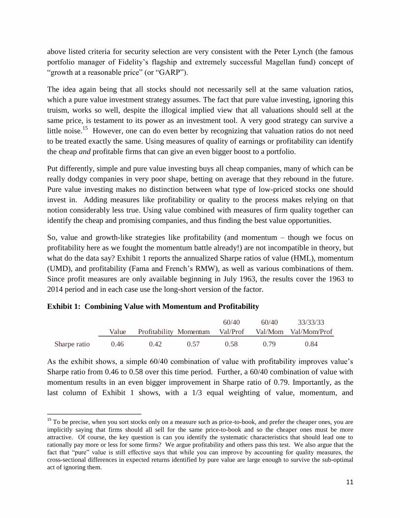
what do the data say? Exhibit 1 reports the annualized Sharpe ratios of value (HML), momentum
(UMD), and profitability (Fama and French’s RMW), as well as various combinations of them.
Since profit measures are only available beginning in July 1963, the results cover the 1963 to
2014 period and in each case use the long-short version of the factor.
Exhibit 1: Combining Value with Momentum and Profitability
As the exhibit shows, a simple 60/40 combination of value with profitability improves value’s
Sharpe ratio from 0.46 to 0.58 over this time period. Further, a 60/40 combination of value with
momentum results in an even bigger improvement in Sharpe ratio of 0.79. Importantly, as the
last column of Exhibit 1 shows, with a 1/3 equal weighting of value, momentum, and
15
To be precise, when you sort stocks only on a measure such as price-to-book, and prefer the cheaper ones, you are
implicitly saying that firms should all sell for the same price-to-book and so the cheaper ones must be more
attractive. Of course, the key question is can you identify the systematic characteristics that should lead one to
rationally pay more or less for some firms? We argue profitability and others pass this test. We also argue that the
fact that “pure” value is still effective says that while you can improve by accounting for quality measures, the
cross-sectional differences in expected returns identified by pure value are large enough to survive the sub-optimal
act of ignoring them.
60/40 60/40 33/33/33
Value Profitability Momentum Val/Prof Val/Mom Val/Mom/Prof
Sharpe ratio 0.46 0.42 0.57 0.58 0.79 0.84
12
profitability, the improvement in Sharpe ratio is even higher at 0.84.16
Hence, a value portfolio’s
Sharpe ratio almost doubles by combining it with growth-like strategies such as momentum and
profitability. Interestingly, using a simple optimizer to choose positive weights on each to
maximize the Sharpe ratio of the portfolio results in weights not too far off from 33% in each.17
While adding measures like profitability to improve a value strategy can still be consistent with
an efficient markets/risk-based view, that story works best if profitability is both negatively
correlated with value and does not carry a positive premium on its own. For example, all-else-
equal, being negatively correlated with (hedging) the value factor should imply a negative
expected return, so if the return is not as negative as expected, or is zero, then it can add
significant diversification benefits. Profitability (and especially momentum) is strongly
negatively correlated with value. However, its returns are not simply zero or less negative than
they should be, but rather are strongly positive. This, of course, makes profitability an even
more valuable factor to add to value, but, at the same time, makes it harder to reconcile from an
efficient markets point of view. If profitability is merely “cleaning up” value, something
consistent with both risk and behavioral stories, then its efficacy on its own would be flat or
neutral. So, given that profitability has a strong positive return premium, it’s also doing
something more by owning higher quality expensive stocks. For proponents of a risk-based view
of the value premium, this presents a challenge since it is these expensive high quality stocks that
also enjoy a positive premium.18
Our view is that most of these factors work for a combination
of reasons – risk and behavioral – and these results fit nicely into that paradigm.
So, whether you are a systematic, diversified value manager or a concentrated value manager,
adding measures of profitability as another bona fide factor can improve your portfolio greatly,
and neither proves or disproves that value is consistent or inconsistent with efficient markets.
Clearly, value does not work best alone. Far from it. And, combining it with other intuitive and
empirically strong factors such as profitability and momentum builds the best portfolio.
16
We note again that these findings are robust to testing in other countries, and for use in other asset classes where
appropriate (momentum always has an analogy for other asset classes, profitability sometimes). 17
Of course, the returns above are to long-short portfolios and all before trading costs and do not include taxes or
other practical costs an investor might face. However, the diversification benefits of combining value with
momentum and profitability also extend to trading costs and tax considerations, and to long-only portfolios
particularly when viewed versus a neutral benchmark (see Frazzini et al. [2012] and Israel and Moskowitz [2013b]).
After taxes and trading costs, the historically optimal portfolio has still been far from pure value, including sizeable
weights to momentum and profitability. 18
Perhaps for this reason, some use profitability (and momentum) as a screen rather than as a separate factor in their
investment process. We covered this ground in our last paper on momentum, so we will only rehash the highlights
here. Basically, the use of other factors as only a screen is an attempt to be a “little pregnant,” because you either
believe in these other factors and hence would want to use them effectively, or you do not believe in them and thus
would not want to use them at all (i.e., you are either pregnant or you are not). Adding only a little bit of a factor via
screens is inconsistent with both and only optimal under the most restrictive conditions that are wildly inconsistent
with the data. And, even if you only believe in another factor “a little” the proper action would be to give it a little
weight in creating your desired portfolio, not to use it as a screen.
13
Fiction: Value is “redundant.”
Fama and French [2014] advance a new Five Factor Model (FFM) that adds a “profitability”
factor (RMW) and an “investment” factor (CMA) to the three factor model of Fama and French
[1993]. Similarly, Asness, Frazzini, and Pedersen [2014] advance a model that adds a composite
“quality” factor that includes within it both profitability and investment related factors which are
commonly considered as part of a firm’s quality..
Some controversy has arisen with regard to the FFM in that the stalwart value factor, HML, is
claimed to be “redundant,” in the sense that it adds nothing beyond the other four factors in
explaining returns. Enough of a stir was created that Fama and French decided to write about it,
explaining “When we say that HML is redundant, what we mean is that its average return is fully
captured by its exposures to the other factors of the five-factor model. This means HML has no
information about average returns that is not in other factors, so we do not need HML to explain
average returns.”19
So, should we all stop worrying about, and writing long papers about, say,
the facts and fictions related to value investing, instead concentrating on only the other four
factors? Should we all stop building investment products with value investing as a core feature
and instead switch to these others? We argue no.
In principle there is nothing wrong with value, as proxied by HML, being captured by other
sources such as a combination of profitability and investment, implying there are simply better
ways to measure and capture the value effect. It would not mean value was useless. It would
simply mean its efficacy could be fully captured in other ways. However, we do not believe
value is redundant in even this way. And, the reason why has to do with two things we have
already discussed along the way: 1) the fact that the Fama-French HML factor, as discussed
above, uses a price that is highly lagged, and 2), in an ironic twist, the one missing factor that
Fama and French have never embraced in their academic work – momentum!
Fama and French [2014] explicitly omits momentum, despite the overwhelming evidence that it
contributes to explaining returns and is itself not captured by the other five factors (e.g.,
momentum is not redundant), while simultaneously keeping value, despite their own evidence
showing that it is driven out by their other factors. The fact that the momentum factor they left
out resurrects the most famous factor everybody associates with them, value, is not only ironic,
but is also very consistent with a long-standing view (emphasized many times in the following
papers: Asness et. al [2014], Asness, Moskowitz, and Pedersen [2013], Asness and Frazzini
[2013], Asness [2011], and Asness et. al [2015]) that value and momentum are best viewed
together, as a system, and not stand-alone. Failure to do so can result in erroneous conclusions
19
See the Fama/French Forum hosted by Dimensional: “Q&A: What does it mean to say HML is redundant?”
(http://www.dimensional.com/famafrench/questions-answers/qa-what-does-it-mean-to-say-hml-is-redundant.aspx.)
14
and poorer investment decisions, of which the apparent “redundancy” of value in the new five
factor world is another example.
To be precise, there are two things that resurrect HML within the new Fama and French five
factor model that are both related to viewing value and momentum together. The first is
including a momentum factor explicitly in the model along with value. The second is to
construct that value factor as discussed earlier by using up-to-date timely, not lagged, measures
of prices, a seemingly small change that turns out to have sizeable consequences.
Here’s the evidence that backs up these claims.20
Exhibit 2 replicates the Fama and French
results where HML is seemingly made redundant by the other factors as found in the first panel
of Table 6 in Fama and French’s [2014] paper. The table reports results from regressing the
monthly returns on each of their factors individually from July 1963 through December 2013 on
the other four factors. In finance geek speak, we are interested in seeing if the two new factors
“subsume” or “span” value, which means asking whether a factor can be essentially replicated by
a linear combination of the other factors. If a factor is so spanned then it is “redundant.”
The first row of Exhibit 2 replicates their version with the sole aesthetic difference being that we
report the intercept in percent per annum.
Each row reports the regression coefficients, with t-statistics below in parentheses. The first
column reports the intercept or alpha from the regressions and the last column the R-squared. If
the intercept is reliably different from zero, e.g., statistically significant at a reasonable level of
confidence usually meaning having an absolute value of its t-statistic > 2, then the dependent
variable factor in question contributes to explaining returns above and beyond the other four
factors. If the intercept is zero (statistically no different from zero), then the other four factors
span or subsume the factor in question. That is, the factor is redundant.
As the first row shows, HML is indeed redundant in this particular model. This is the headliner.
The controversial, or at least somewhat jolting, finding.
20
More details can be found here: https://www.aqr.com/cliffs-perspective/our-model-goes-to-six-and-saves-value-
from-redundancy-along-the-way.
15
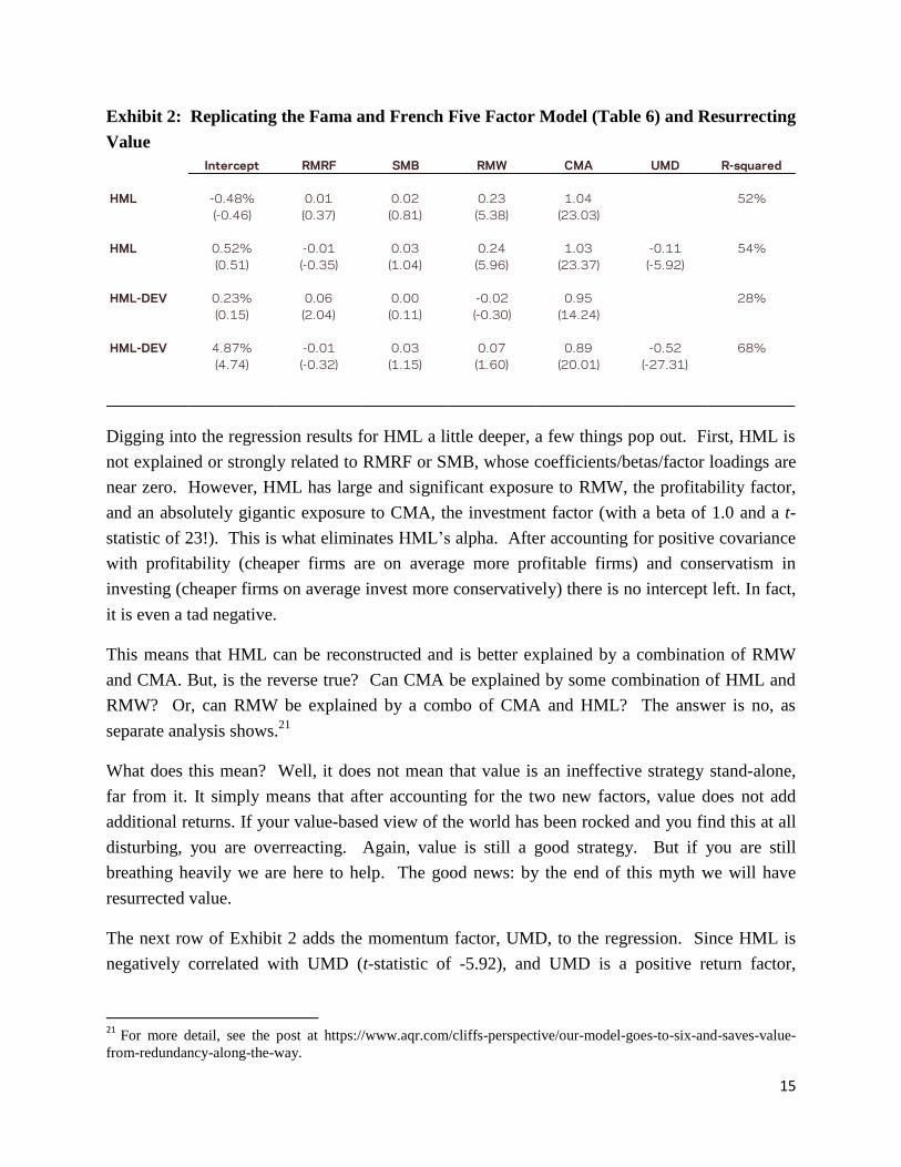
Exhibit 2: Replicating the Fama and French Five Factor Model (Table 6) and Resurrecting
Value
Digging into the regression results for HML a little deeper, a few things pop out. First, HML is
not explained or strongly related to RMRF or SMB, whose coefficients/betas/factor loadings are
near zero. However, HML has large and significant exposure to RMW, the profitability factor,
and an absolutely gigantic exposure to CMA, the investment factor (with a beta of 1.0 and a t-
statistic of 23!). This is what eliminates HML’s alpha. After accounting for positive covariance
with profitability (cheaper firms are on average more profitable firms) and conservatism in
investing (cheaper firms on average invest more conservatively) there is no intercept left. In fact,
it is even a tad negative.
This means that HML can be reconstructed and is better explained by a combination of RMW
and CMA. But, is the reverse true? Can CMA be explained by some combination of HML and
RMW? Or, can RMW be explained by a combo of CMA and HML? The answer is no, as
separate analysis shows.21
What does this mean? Well, it does not mean that value is an ineffective strategy stand-alone,
far from it. It simply means that after accounting for the two new factors, value does not add
additional returns. If your value-based view of the world has been rocked and you find this at all
disturbing, you are overreacting. Again, value is still a good strategy. But if you are still
breathing heavily we are here to help. The good news: by the end of this myth we will have
resurrected value.
The next row of Exhibit 2 adds the momentum factor, UMD, to the regression. Since HML is
negatively correlated with UMD (t-statistic of -5.92), and UMD is a positive return factor,
21
For more detail, see the post at https://www.aqr.com/cliffs-perspective/our-model-goes-to-six-and-saves-value-
from-redundancy-along-the-way.
Intercept RMRF SMB RMW CMA UMD R-squared
HML -0.48% 0.01 0.02 0.23 1.04 52%
(-0.46) (0.37) (0.81) (5.38) (23.03)
HML 0.52% -0.01 0.03 0.24 1.03 -0.11 54%
(0.51) (-0.35) (1.04) (5.96) (23.37) (-5.92)
HML-DEV 0.23% 0.06 0.00 -0.02 0.95 28%
(0.15) (2.04) (0.11) (-0.30) (14.24)
HML-DEV 4.87% -0.01 0.03 0.07 0.89 -0.52 68%
(4.74) (-0.32) (1.15) (1.60) (20.01) (-27.31)
16
HML’s alpha increases by 1% per annum. That is enough to flip its sign but not enough to get it
to statistical significance. So HML is not quite as redundant as before, but not resurrected either.
To save value we are going to have to change it. Fama and French’s industry-standard
construction of HML uses annual rebalancing in June, using book-to-price as the valuation
measure to decide “H” and “L”, where both book and price are taken as of the prior December.
That is, both book and price are six months old upon portfolio formation, and grow to eighteen
months old by the time the portfolio is rebalanced next. Regarding the initial six month lag, there
is a clear reason to do this for the book value: to ensure that an investor would have had this
information in real time when forming a portfolio and therefore the backtested results do not
suffer from look-ahead bias.
But, as discussed earlier, the researcher has a choice as to which price to use. You could use, as
Fama and French did, price from the same date as book so they match in time. However, Asness
and Frazzini [2013] argue for a mismatch in the timing of book and price for two reasons. First,
if all you knew is price fell dramatically (and vice versa for all these examples) since you last
had an accurate matched-in-time book-to-price, your best guess would clearly be that book-to-
price went up because book does not tend to move as much as price. Second, a properly
constructed value strategy is naturally (and to us quite beautifully) negatively correlated with
momentum. Throwing in a six month lag in price that grows to eighteen months before the next
rebalance throws away much of this natural, elegant, and intuitive negative correlation.
After making these arguments Asness and Frazzini [2013] construct an alternative to Fama and
French’s HML by preserving all aspects of their methodology, except allowing the portfolio to
rebalance monthly, using last month’s price to scale book values. In the third row of Exhibit 2
we show the results of re-running the regression by replacing Fama and French’s HML with
HML-DEV. The result, for the most part, is a non-event. HML-DEV experiences an intercept
that is not radically different from using Fama-French HML and still no different from zero. It is
now insignificantly positive instead of insignificantly negative. So it is still redundant.
Now, let us add back momentum in the fourth row of Exhibit 2. Resurrection! Finally, we have
some meaningfully different results, all from doing two simple things.
Timely value, or HML-DEV, now has an economically and statistically large intercept, even
with a very large loading on the positive CMA factor. The negative correlation with the
successful momentum factor is just that powerful. Again, value and momentum are best thought
of as a system. They are both strong alone, but much stronger together due to their negative
correlation (which shows up most clearly when value is defined with timely prices).
17
Fama and French’s latest Five Factor Model may be a useful way to summarize the known
playing field of factors, and it brings some very good things to the table. However, for reasons
we do not find compelling, it leaves out momentum. With no change necessary to the value
factor it is absolutely compelling to add momentum back, creating a better Six Factor Model.
But, as we have argued for some time, the value factor can be made timelier. Doing so makes
momentum even stronger, and the value factor, rendered distressingly (for those of us who have
considered ourselves value investors for many years) redundant by the Five Factor Model, is
suddenly and clearly resurrected.
Strong proponents of pure value may rejoice at this news, but at the same time they must face the
irony that it was momentum that rescued them.
Fact: Value investing is applicable to more than just choosing what stocks to own or avoid.
Can value really be applied outside of equities? To many, value is a concept that applies
exclusively to stocks, in part because most of the academic literature and evidence has focused
on stocks and, relatedly, because the most common way people measure value is by some ratio
of accounting-value-to-market-value, such as the book-to-market equity ratio. Since accounting
values are non-existent in other asset classes such as bonds, commodities, currencies, etc. value
is often thought not to apply to those assets.
But, we can think more broadly about what value investing is trying to accomplish: identify
cheap versus expensive assets. If we can measure cheapness and expensiveness in other asset
classes, then we can form a value portfolio in other asset classes. There are many reasonable
ways to measure value, including reversal of long-term past returns. And, as every asset has a
measureable return, this is at least one measure of value we can use for any asset class.
In other asset classes, we can form direct fundamental measures of value as well. For instance, in
bonds a measure of value is the real bond yield or yield on a bond minus expected inflation. For
currencies, deviations from purchasing power parity (PPP) as proxied by the price of a basket of
goods in two countries relative to their exchange rate might also indicate cheapness and
expensiveness, as in the long-run exchange rates should converge to PPP across countries.
Using some of these value measures, Asness et al. [2013] document significant value return
premia in bonds, country equity index futures, commodities, currencies, and equities globally,
from 1972 to 2011. They find not only that there is a reliable value premium in each asset class,
but that the correlation of value strategies across asset classes is positive. Interestingly, the value
strategy correlations are higher than passive exposures to the asset classes themselves, indicating
that value strategies in different asset classes using different measures, but all tied together by the
same theme of identifying cheap versus expensive assets, are still capturing a similar
phenomenon. In other words, cheap assets in one asset class move with cheap assets in other
asset classes, bonded by an overall value effect that pervades all of these markets.
18
So, value is more than a narrowly defined equity-only concept and can be applied more broadly
to any asset class. The implications of this are that more robust and diversified value strategies
can be created that deliver better and more stable performance. Asness et al. [2013] show that a
diversified value strategy applied across all asset classes more than doubles the Sharpe ratio of a
U.S. equity-only value strategy such as HML. Moreover, combining value with momentum, and
doing so across all asset classes, improves an overall portfolio by substantially more.
Regardless of whether one takes advantage of these global (across geography and asset class)
results, they are out-of-sample tests of the original U.S. results, which makes us more confident
that both value and momentum are effective and even more effective together rather than
separately, a robust feature of the data and not an artifact of data mining.
Fact: Value can be measured in many ways, and is best measured by a composite of
variables.
Simple intuition tells you this should be true. The opposite idea that a single measure of
anything is optimal – given estimation error, data mining concerns, and absent any strong theory
– seems at best remote and most likely wrong.
Nevertheless, we put this statement to the test in the data. The predominant, certainly in
academia, way to measure value is to use the book value of a firm’s equity relative to its market
value, referred to as the book-to-market ratio, or expressed per share as book-to-price. This
particular measure of value has been made popular by Fama and French [1992, 1993, 1996,
2008, and 2012] in a series of papers. But, we know of no theoretical justification for it as the
true measure of value versus other reasonable competitors. In fact, Fama and French [1996] use
a variety of fundamental-to-price ratios, such as earnings-to-price and cash flow-to-price, and
other measures of value such as dividend yield, sales growth, and even reversal of the past five-
year returns (the “poor man’s” value measure).
The results are consistent across measures, and the portfolios constructed from different value
measures yield highly correlated returns. Exhibit 3 reports summary statistics on HML-style
portfolios using different value measures to rank stocks. These portfolios are taken from Kenneth
French’s website and pertain to the top 30% of stocks (value stocks) minus the bottom 30% of
stocks (growth stocks) based on book-to-market equity (BE/ME), earnings-to-price (E/P), cash
flow-to-price (CF/P), dividend yield (D/P), and negative past five-year returns.
While there is some variation in returns across the different measures, all of the HML-style
portfolios based on different value measures produce positive returns and are highly correlated.
19
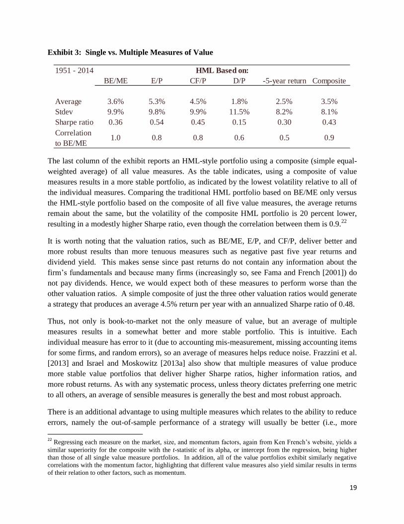
Exhibit 3: Single vs. Multiple Measures of Value
The last column of the exhibit reports an HML-style portfolio using a composite (simple equal-
weighted average) of all value measures. As the table indicates, using a composite of value
measures results in a more stable portfolio, as indicated by the lowest volatility relative to all of
the individual measures. Comparing the traditional HML portfolio based on BE/ME only versus
the HML-style portfolio based on the composite of all five value measures, the average returns
remain about the same, but the volatility of the composite HML portfolio is 20 percent lower,
resulting in a modestly higher Sharpe ratio, even though the correlation between them is 0.9.22
It is worth noting that the valuation ratios, such as BE/ME, E/P, and CF/P, deliver better and
more robust results than more tenuous measures such as negative past five year returns and
dividend yield. This makes sense since past returns do not contain any information about the
firm’s fundamentals and because many firms (increasingly so, see Fama and French [2001]) do
not pay dividends. Hence, we would expect both of these measures to perform worse than the
other valuation ratios. A simple composite of just the three other valuation ratios would generate
a strategy that produces an average 4.5% return per year with an annualized Sharpe ratio of 0.48.
Thus, not only is book-to-market not the only measure of value, but an average of multiple
measures results in a somewhat better and more stable portfolio. This is intuitive. Each
individual measure has error to it (due to accounting mis-measurement, missing accounting items
for some firms, and random errors), so an average of measures helps reduce noise. Frazzini et al.
[2013] and Israel and Moskowitz [2013a] also show that multiple measures of value produce
more stable value portfolios that deliver higher Sharpe ratios, higher information ratios, and
more robust returns. As with any systematic process, unless theory dictates preferring one metric
to all others, an average of sensible measures is generally the best and most robust approach.
There is an additional advantage to using multiple measures which relates to the ability to reduce
errors, namely the out-of-sample performance of a strategy will usually be better (i.e., more
22
Regressing each measure on the market, size, and momentum factors, again from Ken French’s website, yields a
similar superiority for the composite with the t-statistic of its alpha, or intercept from the regression, being higher
than those of all single value measure portfolios. In addition, all of the value portfolios exhibit similarly negative
correlations with the momentum factor, highlighting that different value measures also yield similar results in terms
of their relation to other factors, such as momentum.
1951 - 2014
BE/ME E/P CF/P D/P -5-year return Composite
Average 3.6% 5.3% 4.5% 1.8% 2.5% 3.5%
Stdev 9.9% 9.8% 9.9% 11.5% 8.2% 8.1%
Sharpe ratio 0.36 0.54 0.45 0.15 0.30 0.43
Correlation
to BE/ME1.0 0.8 0.8 0.6 0.5 0.9
HML Based on:
20
closely match the backtest) when using an average of multiple measures. As with any specific
sample of data, you will always find some measures that work particularly well in sample and
some that do not (e.g., E/P vs. D/P in Exhibit 3). However, without theory telling you a priori
why one measure should outperform another, this is largely due to chance. As a consequence,
you would not expect that same measure to outperform out-of-sample. Taking an average of
multiple measures guards against picking one particular measure over others that happened to
work well in one particular sample. In other words, it helps prevent data mining by extracting
more of the signal and avoiding over fitting errors.
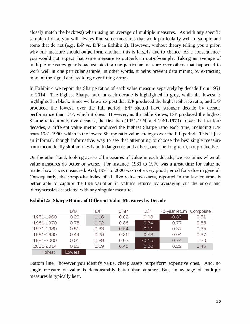
In Exhibit 4 we report the Sharpe ratios of each value measure separately by decade from 1951
to 2014. The highest Sharpe ratio in each decade is highlighted in grey, while the lowest is
highlighted in black. Since we know ex post that E/P produced the highest Sharpe ratio, and D/P
produced the lowest, over the full period, E/P should have stronger decade by decade
performance than D/P, which it does. However, as the table shows, E/P produced the highest
Sharpe ratio in only two decades, the first two (1951-1960 and 1961-1970). Over the last four
decades, a different value metric produced the highest Sharpe ratio each time, including D/P
from 1981-1990, which is the lowest Sharpe ratio value strategy over the full period. This is just
an informal, though informative, way to see that attempting to choose the best single measure
from theoretically similar ones is both dangerous and at best, over the long-term, not productive.
On the other hand, looking across all measures of value in each decade, we see times when all
value measures do better or worse. For instance, 1961 to 1970 was a great time for value no
matter how it was measured. And, 1991 to 2000 was not a very good period for value in general.
Consequently, the composite index of all five value measures, reported in the last column, is
better able to capture the true variation in value’s returns by averaging out the errors and
idiosyncrasies associated with any singular measure.
Exhibit 4: Sharpe Ratios of Different Value Measures by Decade
Bottom line: however you identify value, cheap assets outperform expensive ones. And, no
single measure of value is demonstrably better than another. But, an average of multiple
measures is typically best.
B/M E/P CF/P D/P -5-year return Composite
1951-1960 0.28 1.16 0.82 0.08 -0.83 0.51
1961-1970 0.78 1.02 0.86 0.34 0.77 0.85
1971-1980 0.51 0.33 0.54 -0.11 0.37 0.35
1981-1990 0.44 0.29 0.26 0.48 0.04 0.37
1991-2000 0.01 0.39 0.03 -0.15 0.74 0.20
2001-2014 0.28 0.39 0.45 0.30 0.29 0.45
Highest Lowest
21
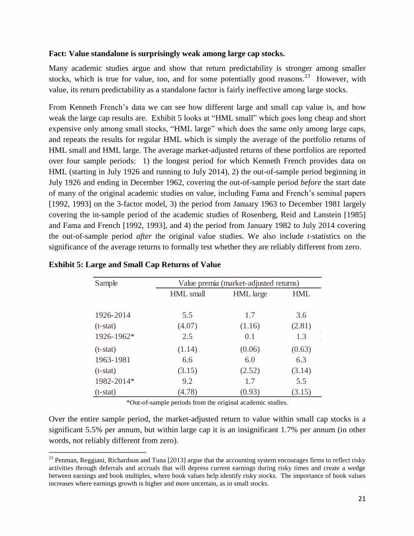
Fact: Value standalone is surprisingly weak among large cap stocks.
Many academic studies argue and show that return predictability is stronger among smaller
stocks, which is true for value, too, and for some potentially good reasons.23
However, with
value, its return predictability as a standalone factor is fairly ineffective among large stocks.
From Kenneth French’s data we can see how different large and small cap value is, and how
weak the large cap results are. Exhibit 5 looks at “HML small” which goes long cheap and short
expensive only among small stocks, “HML large” which does the same only among large caps,
and repeats the results for regular HML which is simply the average of the portfolio returns of
HML small and HML large. The average market-adjusted returns of these portfolios are reported
over four sample periods: 1) the longest period for which Kenneth French provides data on
HML (starting in July 1926 and running to July 2014), 2) the out-of-sample period beginning in
July 1926 and ending in December 1962, covering the out-of-sample period before the start date
of many of the original academic studies on value, including Fama and French’s seminal papers
[1992, 1993] on the 3-factor model, 3) the period from January 1963 to December 1981 largely
covering the in-sample period of the academic studies of Rosenberg, Reid and Lanstein [1985]
and Fama and French [1992, 1993], and 4) the period from January 1982 to July 2014 covering
the out-of-sample period after the original value studies. We also include t-statistics on the
significance of the average returns to formally test whether they are reliably different from zero.
Exhibit 5: Large and Small Cap Returns of Value
*Out-of-sample periods from the original academic studies.
Over the entire sample period, the market-adjusted return to value within small cap stocks is a
significant 5.5% per annum, but within large cap it is an insignificant 1.7% per annum (in other
words, not reliably different from zero).
23
Penman, Reggiani, Richardson and Tuna [2013] argue that the accounting system encourages firms to reflect risky
activities through deferrals and accruals that will depress current earnings during risky times and create a wedge
between earnings and book multiples, where book values help identify risky stocks. The importance of book values
increases where earnings growth is higher and more uncertain, as in small stocks.
Sample
HML small HML large HML
1926-2014 5.5 1.7 3.6
(t-stat) (4.07) (1.16) (2.81)
1926-1962* 2.5 0.1 1.3
(t-stat) (1.14) (0.06) (0.63)
1963-1981 6.6 6.0 6.3
(t-stat) (3.15) (2.52) (3.14)
1982-2014* 9.2 1.7 5.5
(t-stat) (4.78) (0.93) (3.15)
Value premia (market-adjusted returns)
22
Looking at the sub period results, the only period where there seems to be a significantly positive
HML premium among large cap stocks is over the in-sample period from 1963-1981, when the
bulk of the original academic work on value took place. Over both out-of-sample periods – prior
to these studies from 1926 to 1962 and after these studies from 1982 to 2014 – there is no
evidence that there exists a healthy value premium among large cap stocks. Even over the entire
88-year sample period that includes the in-sample evidence, HML among large cap stocks does
not yield significantly positive returns!24
This may come as a surprise to some readers who only remember the original academic studies
using data from 1963 to the early 1980s where large cap value does seem to work. However,
upon further review and revisiting the data and updating the analysis, there is not, or perhaps
there never was, a strong stand-alone value premium among large caps.
Pushing this a bit further also reveals something not generally appreciated about the construction
of HML (the benchmark by which most researchers measure value). HML, which is an equal-
weighted combination of HML small and HML large, by construction gives much more weight
to small than a simple passive cap-weighted value portfolio would, leading to better looking
results. The last column of Exhibit 5 shows that HML looks alive and well in every period
except 1926 to 1962, even though small cap HML performed well. While HML is touted and
used as a benchmark and often thought of as a passive portfolio, it is actually a monthly
rebalanced equal-weighted portfolio of small cap HML and large cap HML, whereby giving 50%
weight to small cap HML significantly overweights exposure to small cap value relative to a cap
weighted value benchmark. Furthermore, since the risk of small cap stocks is higher than large
caps, the exposure to small caps is even greater and more imbalanced from a risk perspective. A
purely cap-weighted value portfolio with market-cap weights would look much like HML large,
as the large stocks would dominate in cap-weighting which does not reveal a significant return
premium over the full sample period (it would likely look slightly better as it would have very
small, but positive, exposure to smaller stocks).
Despite the weakness of the large cap results, we are still big proponents of value investing even
among large cap stocks. Why? Because the weak stand-alone evidence of large cap value should
not be confused with value’s very valuable contribution to a portfolio, particularly one with
momentum or profitability in it as we showed earlier.
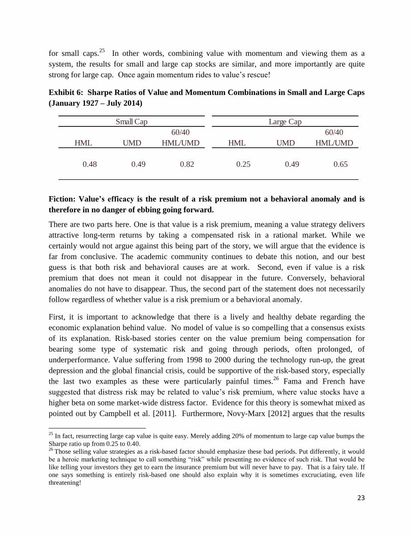
Exhibit 6 separately looks at small and large cap value in combination with momentum. Even
though the small cap value strategy has the higher Sharpe ratio, it is still greatly improved by
combining it with momentum – raising the Sharpe ratio from 0.48 to 0.82. But, for large cap
value, which by itself only generates a 0.25 Sharpe ratio, combining it with large cap momentum
produces a robust 0.65 Sharpe, which is not so far off the combination of value and momentum
24
For a more detailed study on this topic, see Israel and Moskowitz [2013a], who find that the value premium is
virtually non-existent among large stocks.
23
for small caps.25
In other words, combining value with momentum and viewing them as a
system, the results for small and large cap stocks are similar, and more importantly are quite
strong for large cap. Once again momentum rides to value’s rescue!
Exhibit 6: Sharpe Ratios of Value and Momentum Combinations in Small and Large Caps
(January 1927 – July 2014)
Fiction: Value’s efficacy is the result of a risk premium not a behavioral anomaly and is
therefore in no danger of ebbing going forward.
There are two parts here. One is that value is a risk premium, meaning a value strategy delivers
attractive long-term returns by taking a compensated risk in a rational market. While we
certainly would not argue against this being part of the story, we will argue that the evidence is
far from conclusive. The academic community continues to debate this notion, and our best
guess is that both risk and behavioral causes are at work. Second, even if value is a risk
premium that does not mean it could not disappear in the future. Conversely, behavioral
anomalies do not have to disappear. Thus, the second part of the statement does not necessarily
follow regardless of whether value is a risk premium or a behavioral anomaly.
First, it is important to acknowledge that there is a lively and healthy debate regarding the
economic explanation behind value. No model of value is so compelling that a consensus exists
of its explanation. Risk-based stories center on the value premium being compensation for
bearing some type of systematic risk and going through periods, often prolonged, of
underperformance. Value suffering from 1998 to 2000 during the technology run-up, the great
depression and the global financial crisis, could be supportive of the risk-based story, especially
the last two examples as these were particularly painful times.26
Fama and French have
suggested that distress risk may be related to value’s risk premium, where value stocks have a
higher beta on some market-wide distress factor. Evidence for this theory is somewhat mixed as
pointed out by Campbell et al. [2011]. Furthermore, Novy-Marx [2012] argues that the results
25
In fact, resurrecting large cap value is quite easy. Merely adding 20% of momentum to large cap value bumps the
Sharpe ratio up from 0.25 to 0.40. 26
Those selling value strategies as a risk-based factor should emphasize these bad periods. Put differently, it would
be a heroic marketing technique to call something “risk” while presenting no evidence of such risk. That would be
like telling your investors they get to earn the insurance premium but will never have to pay. That is a fairy tale. If
one says something is entirely risk-based one should also explain why it is sometimes excruciating, even life
threatening!
60/40 60/40
HML UMD HML/UMD HML UMD HML/UMD
0.48 0.49 0.82 0.25 0.49 0.65
Small Cap Large Cap
24
on firm profitability and its interaction with value provide a real challenge to the distress risk
story. We have hit on this earlier. If something (value) is purely a distress premium it would be
odd that you can mitigate that distress (buying stronger more profitable companies) and get paid
to do so. Typically, you have to pay to alleviate risk, not get paid, so, if profitability was a
negative return that hedged value and thus was useful it would be a more consistent story. In
addition, the notion of distress is hard to reconcile with the evidence on value effects in
commodities, for example, where it is difficult to think of what “distress” means.
The behavioral theories focus on investor mis-reaction to information that causes temporary
mispricing. For value, a leading story, originally suggested by DeBondt and Thaler [1985] and
Lakonishok et al. [1994] and later formalized by Daniel et al. [1998], is that the value premium is
driven by investor overreaction. The idea is that value stocks are neglected stocks that investors
have fled from and now shun, while growth stocks are glamour stocks that investors have
irrationally stampeded toward, causing value stocks to be underpriced and growth stocks to be
overpriced. This story, while formulated before it, is often seen to be buoyed by the technology
boom and bust of the late 1990’s to early 2000’s and the corresponding bust and boom of value.
Academics from the rational-risk-based-efficient markets camp continue to wage war with
academics from the behavioral-irrational-inefficient markets group over what drives the value
premium. While the jury is still out on which of these explanations better fit the data (indeed, the
2013 Nobel Prize committee split the prize between the two camps),27
almost all agree that the
data are undeniable – value offers a robust return premium highly unlikely to be the random
result of data mining. And, in our view, both theories have some truth to them as is likely the
case with most other premia. The world is rarely so bright-lined that one theory is correct and
the other completely wrong. Elements of both risk and behavior are likely present.
Furthermore, to make things more interesting, or more complicated depending on your
perspective, if both explanations have important elements of truth and make up part of the story,
nothing says that mix is constant through time. For instance, inefficiency-based behavioral type
reasons may have driven much of the 1999-2000 period where value suffered at historic levels,
and then soared at historic levels, but that could be the exception that proves the rule. The
important point, however, is that both theories offer good reasons to expect the value premium to
persist in the future.
If value is a risk premium, however, would that imply that we do not expect it to disappear (and
its subtext: if not risk, then would it disappear)? Just because something is related to risk (and
we reiterate that for value this is far from certain) does not guarantee it will not get greatly
reduced. If risks change or the taste or compensation for risk changes, then so, too, will the
expected returns to that risk. Critics of efficient markets have long mistaken time-varying risk
premia for a refutation of the idea of efficient markets based risk premia. As long as risks and
27
Asness and Liew [2014] give a thorough discussion of this from both academic and practitioner perspectives.
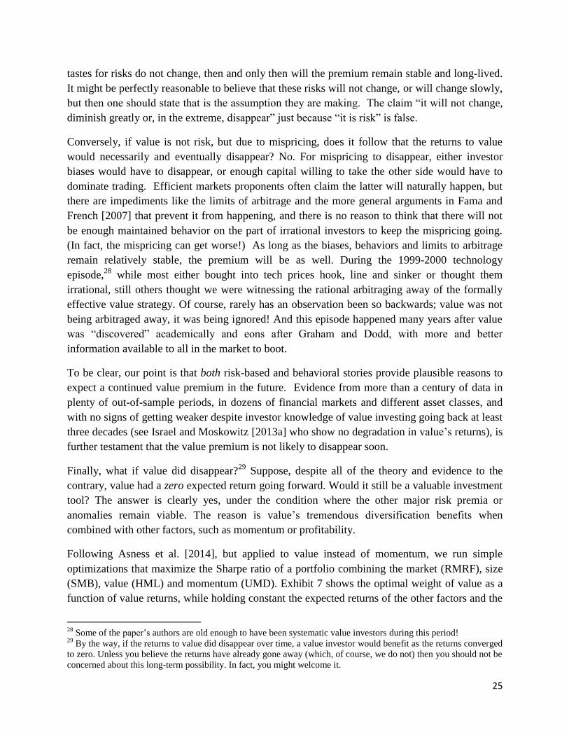
25
tastes for risks do not change, then and only then will the premium remain stable and long-lived.
It might be perfectly reasonable to believe that these risks will not change, or will change slowly,
but then one should state that is the assumption they are making. The claim “it will not change,
diminish greatly or, in the extreme, disappear” just because “it is risk” is false.
Conversely, if value is not risk, but due to mispricing, does it follow that the returns to value
would necessarily and eventually disappear? No. For mispricing to disappear, either investor
biases would have to disappear, or enough capital willing to take the other side would have to
dominate trading. Efficient markets proponents often claim the latter will naturally happen, but
there are impediments like the limits of arbitrage and the more general arguments in Fama and
French [2007] that prevent it from happening, and there is no reason to think that there will not
be enough maintained behavior on the part of irrational investors to keep the mispricing going.
(In fact, the mispricing can get worse!) As long as the biases, behaviors and limits to arbitrage
remain relatively stable, the premium will be as well. During the 1999-2000 technology
episode,28
while most either bought into tech prices hook, line and sinker or thought them
irrational, still others thought we were witnessing the rational arbitraging away of the formally
effective value strategy. Of course, rarely has an observation been so backwards; value was not
being arbitraged away, it was being ignored! And this episode happened many years after value
was “discovered” academically and eons after Graham and Dodd, with more and better
information available to all in the market to boot.
To be clear, our point is that both risk-based and behavioral stories provide plausible reasons to
expect a continued value premium in the future. Evidence from more than a century of data in
plenty of out-of-sample periods, in dozens of financial markets and different asset classes, and
with no signs of getting weaker despite investor knowledge of value investing going back at least
three decades (see Israel and Moskowitz [2013a] who show no degradation in value’s returns), is
further testament that the value premium is not likely to disappear soon.
Finally, what if value did disappear?29
Suppose, despite all of the theory and evidence to the
contrary, value had a zero expected return going forward. Would it still be a valuable investment
tool? The answer is clearly yes, under the condition where the other major risk premia or
anomalies remain viable. The reason is value’s tremendous diversification benefits when
combined with other factors, such as momentum or profitability.
Following Asness et al. [2014], but applied to value instead of momentum, we run simple
optimizations that maximize the Sharpe ratio of a portfolio combining the market (RMRF), size
(SMB), value (HML) and momentum (UMD). Exhibit 7 shows the optimal weight of value as a
function of value returns, while holding constant the expected returns of the other factors and the
28
Some of the paper’s authors are old enough to have been systematic value investors during this period! 29
By the way, if the returns to value did disappear over time, a value investor would benefit as the returns converged
to zero. Unless you believe the returns have already gone away (which, of course, we do not) then you should not be
concerned about this long-term possibility. In fact, you might welcome it.
26
correlations between factors at their long-term averages (1927-2014). Using the average value
premium observed in the full sample, the optimization would place about 33% of a portfolio in
HML. Moreover, the exhibit shows that even in the extreme case where we assume a zero return
for value, the optimal portfolio still places a significant positive weight on value (about 13%).
The logic is simple. Since momentum is a good strategy and value is significantly negatively
correlated with it, you would expect value to lose money, and the fact that it breaks even makes
it a valuable hedge. The diversification benefits are so great that even a zero expected return
would be valuable to your portfolio. . Even with the assumption that the value premium goes
away but the momentum premium remains, we think this is strong testimony to the power of
diversification across negatively correlated strategies.
Another point that is often missed is that not every investor can (or should if it’s a risk) hold
value (or tilt towards value). Remember, all investment has to, by definition, aggregate to the
market. So, for every value investor there has to be a growth investor willing to take the other
side. If not, and everyone decided to tilt towards value stocks and away from growth stocks,
then the value premium would cease to exist.
For both explanations of the value premium, therefore, a key component is “who is on the other
side?” In the case of the behavioral stories, it is clear: those who suffer from behavioral biases
or like to chase the glamorous growth stocks and neglect the fallen value stocks. As long as
enough of them continue to survive, the value premium remains intact. For the risk-based
explanation, the answer is investors who do not want to bear the risk associated with value, or
more accurately, those who would pay not to bear it. That is, investors who are long value are
provided a risk premium, like an insurance premium, by those willing to pay for this insurance
(who are naturally short or underweight value). Of course, again, to fully understand this
insurance based explanation we need to fully understand what catastrophe some investors are
rationally insuring against.
This then begs the question: if a manager offering value to its clients believes it is related to risk,
then why not also offer a growth fund for those wishing to bear less of this risk? In other words,
if HML provides a risk premium to investors willing to bear value’s risk, should they not also
offer LMH to the other set of investors who are willing to pay to eliminate this risk? To our
knowledge, no one does (at least explicitly).
27
Exhibit 7: Optimal Weight Frontier for Value
In summary, the jury is still out as to whether the value premium exists because of risk or
behavioral based explanations, and we believe the truth is likely a combination of the two. But,
both theories give a plausible reason to expect a value premium to continue to persist.
Conclusion
Despite being around practically forever and formally studied for at least thirty years there is still
a lot of confusion surrounding value investing. Now that you have seen the evidence, know
where to find it, and can replicate it yourself, hopefully the truth behind value investing will be
clearer.
As we stated before, if one wants to challenge the evidence, that is fine, too. As always, if
someone discovers something challenging or enlightening versus what we have shown, we
welcome it and wish to understand it.
Bottom line: in dispelling the myths about momentum in our prior paper, and detailing the facts
and fictions about value in this one, we end up even stronger believers in both factors, and in
particular their efficacy when used together.
0%
5%
10%
15%
20%
25%
30%
35%
40%
45%
50%
-2% -1% 0% 1% 2% 3% 4% 5% 6% 7% 8% 9% 10%
Op
tim
al p
ort
folio
we
igh
t o
n H
ML
Expected return to HML
28
References
Arnott, R., J. Hsu, and P. Moore [2004]. “Fundamental Indexation.” Financial Analysts Journal:
83-99.
Arnott, R. [2006]. “An Overwrought Orthodoxy.” Institutional Investor, December: 36-41.
Arnott, R., J. Hsu, and J. West [2008]. The Fundamental Index. New Jersey: John Wiley & Sons,
Inc.
Asness, C. [1997]. “The Interaction of Value and Momentum Strategies.” Financial Analysts
Journal, Vol. 53, No. 2, 29-36.
Asness, C. [2006]. “The Value of Fundamental Indexing.” Institutional Investor, October 2006:
94-99.
Asness, C. [2012]. “Momentum in Japan.” Journal of Portfolio Management, Vol. 37, No. 4, 67-
75.
Asness, C. and A. Frazzini [2013]. “The Devil in HML’s Details.” Journal of Portfolio
Management 39(4), 49-68.
Asness, C., A. Frazzini, R. Israel and T. Moskowitz [2014]. “Fact, Fiction, and Momentum
Investing,” Journal of Portfolio Management, 40th Anniversary edition.
Asness, C., A. Frazzini and L. Pedersen [2014]. “Quality Minus Junk.” Working Paper, AQR
Capital Management.
Asness, C., J. Friedman, R. Krail, and J. Liew [2000]. “Style Timing: Value versus Growth”.
Journal of Portfolio Management, volume 26, number 3, 50-60.
Asness, C., A. Ilmanen, R. Israel and T. Moskowitz [2015]. “Investing with Style.” Journal of
Investment Management Volume 13, No. 1, 27–63.
Asness, C. and J. Liew [2014]. “The Great Divide over Market Efficiency.” Institutional
Investor, March 2014.
Asness, C., T. Moskowitz, and L. Pedersen [2013]. ‘‘Value and Momentum Everywhere.’’
Journal of Finance 68(3), 929-985.
Barberis, N., A. Shleifer, and R. Vishny [1998]. “A Model of Investor Sentiment.” Journal of
Financial Economics 49, 307-34.
Bergstresser, D. and J. Pontiff [2013]. “Investment Taxation and Portfolio Performance.” Journal
of Public Economics 97, 245-257.
Berk, J., R. Green, and V. Naik [1999]. “Optimal Investment, Growth Options, and Security
Returns.” Journal of Finance 54, 1553-1607.
Booth, D. [2013]. “The Evolution of Dimensional.” Equius Partners, Inc. Asset Class Newsletter.
29
Campbell, John, Jens Hilscher, and Jan Szilagyi [2011]. “Predicting Financial Distress and the
Performance of Distressed Stocks”, Journal of Investment Management 9(2):1-21.
Carhart, M. [1997]. “On Persistence in Mutual Fund Performance.” Journal of Finance 53.
Chabot, B., E. Ghysels and R. Jagannathan [2009]. “Price Momentum in Stocks: Insights from
Victorian Age Data.” National Bureau of Economic Research Working Papers 14500.
Chabot, B., E. Ghysels and R. Jagannathan [2015]. “Momentum Trading, Return Chasing, and
Predictable Crashes.” Working paper, Northwestern University.
Chan, L., N. Jegadeesh, and J. Lakonishok [1997]. “Momentum strategies.” Journal of Finance,
51, pp. 1681–1713.
Daniel, K., D. Hirshleifer, and A. Subrahmanyam [1998]. “A Theory of Overconfidence, Self-
Attribution, and Security Market Under- and Over-Reactions.” Journal of Finance 53, 1839-
1885.
Daniel, K. and T. Moskowitz [2013]. “Momentum Crashes.” Working paper, University of
Chicago.
DeBondt W., and R. Thaler (1985). “Does the Stock Market Overreact?” Journal of Finance,
40(3), 793-805.
DeLong, J.B., A. Shleifer, L. H. Summers, and R.J. Waldmann [1990]. “Positive Feedback
Investment Strategies and Destabilizing Rational Speculation.” Journal of Finance, 45(2),
379-395.
Erb, Claude B. [2014]. “Momentum Has Not Been 'Overgrazed': A Visual Overview in 10
Slides.” Working paper, SSRN.
Fama, E.F., and K.R. French [1992]. “The cross-section of expected stock returns.” Journal of
Finance 47, 427–465.
Fama, E.F. and K.R. French [1993]. “Common Risk Factors in the Returns on Stocks and
Bonds.” Journal of Financial Economics 33, 3-56.
Fama, E.F. and K.R. French [2001]. “Disappearing dividends: changing firm characteristics or
lower propensity to pay?” Journal of Financial Economics 60(1):3-43.
Fama, E.F. and K.R. French [2007]. “Disagreement, tastes, and asset prices.” Journal of
Financial Economics 83(3):667-689.
Fama, E.F. and K.R. French [2008]. “Dissecting Anomalies.” Journal of Finance 63.
Fama, E.F. and K.R. French [2012]. “Size, Value, and Momentum in International Stock
Returns.” Journal of Financial Economics 105 p. 457-472.
Fama, E.F. and K.R. French [2014]. “A Five-Factor Asset Pricing Model.” Working paper,
University of Chicago.
30
Frazzini, A. [2006]. “The Disposition Effect and Underreaction to News.” Journal of Finance,
61.
Frazzini, A., R. Israel, and T.J. Moskowitz [2012]. “Trading Costs of Asset Pricing Anomalies.”
Working paper, University of Chicago.
Frazzini, A., R. Israel, T.J. Moskowitz and R. Novy-Marx [2013]. “A New Core Equity
Paradigm.” Whitepaper, AQR Capital Management.
Frazzini A., D. Kabiller, and Lasse Heje Pedersen [2013]. “Buffett’s Alpha.” Working paper,
AQR Capital Management.
Geczy, C. and M. Samonov [2013]. “212 Years of Price Momentum (The World’s Longest
Backtest: 1801 – 2012).” Working paper, University of Pennsylvania - The Wharton School.
Goyal, A. and S. Wahal [2013]. “Is Momentum an Echo?” Journal of Financial and Quantitative
Analysis, forthcoming.
Graham, Benjamin [1973]. The Intelligent Investor. 4th ed. New York: Harper.
Graham, Benjamin and David L. Dodd [2009]. Security Analysis. 6th ed. New York: McGraw
Hill.
Greiner, Steven P. [2011]. Ben Graham Was a Quant. New Jersey: John Wiley & Sons, Inc.
Grinblatt, M. and B. Han [2005]. “Prospect Theory, Mental Accounting, and Momentum.”
Journal of Financial Economics.
Grinblatt, M. and T.J. Moskowitz [2004]. “Predicting Stock Price Movements from Past Returns:
The Role of Consistency and Tax-Loss Selling.” Journal of Financial Economics, 71, 541-
579.
Harvey, C., Y. Liu and H. Zhu [2014]. “…and the Cross-Section of Expected Returns”, Working
paper, Duke University Fuqua School of Business.
Hong, H., T. Lim, and J. Stein [2000]. “Bad news travels slowly: size, analyst coverage, and the
profitability of momentum strategies.” Journal of Finance, 55, 265–295.
Hong, H. and J. Stein [1999]. “A Unified Theory of Underreaction, Momentum Trading and
Overreaction in Asset Markets.” Journal of Finance, LIV, no. 6.
Huij, H., S. Lansdorp, D. Blitz, and P. Stein [2014]. “Factor Investing: Long-Only versus Long-
Short.” Working paper, Erasmus School of Economics.
Israel, R. and T. Moskowitz [2012]. “How Tax Efficient Are Equity Styles?” Working paper,
University of Chicago Booth School of Business.
Israel, R. and T. Moskowitz [2013]. “The Role of Shorting, Firm Size, and Time on Market
Anomalies.” Journal of Financial Economics 108(2), 275-301.
31
Jegadeesh, N. and S. Titman [1993]. “Returns to Buying Winners and Selling Losers:
Implications for Stock Market Efficiency.” Journal of Finance, vol. 48, pp. 65-91.
Johnson, Timothy [2002]. “Rational Momentum Effects.” Journal of Finance 57, 585 – 608.
Kahneman, D. and A. Tversky [1979]. “Prospect Theory: An Analysis of Decision Under Risk.”
Econometrica 47.
Keim, D.B. [1999], “An analysis of mutual fund design: the case of investing in small-cap
stocks,” Journal of Financial Economics, vol. 51, pp. 173-194.
Korajczyk, Robert A., and Ronnie Sadka [2004], “Are momentum profits robust to trading
costs?,” Journal of Finance, vol. 59, pp. 1039-1082.
Lakonishok, J., A. Shleifer, and R.W. Vishny (1994). “Contrarian Investment, Extrapolation, and
Risk.” Journal of Finance 49, 1541-1578.
Larson, R. [2013]. “Hot Potato: Momentum as an Investment Strategy.” Research Affiliates
Fundamentals Newsletter.
Lesmond, David A., Michael J. Schill, and Chunsheng Zhou [2003]. “The illusory nature of
momentum profits.” Journal of Financial Economics, vol. 71, pp. 349–380.
Merton, Robert C. [1987]. “A Simple Model of Capital Market Equilibrium with Incomplete
Information.” Journal of Finance 42, 483-510.
Novy-Marx, Robert [2012]. “Is Momentum Really Momentum?” Journal of Financial
Economics, 103(3), 429-453.
Pastor, L. and R. F. Stambaugh [2003]. “Liquidity Risk and Expect Stock Returns.” Journal of
Political Economy, Vol. 111.
Penman, S., F. Reggiani, S. Richardson, A. Irem Tuna [2013]. “An Accounting-Based
Characteristic Model for Asset Pricing.” Working paper, Columbia University.
Rosenberg, R., K. Reid, and R. Lanstein [1985]. “Persuasive Evidence of Market Inefficiency.”
Journal of Portfolio Management, volume 11, number 3, 9-16.
Sagi, J. and M.S. Seasholes [2007]. “Firm-Specific Attributes and the Cross-Section of
Momentum.” Journal of Financial Economics 84, 389-434.
Shefrin, H. and M. Statman [1985]. “The Disposition to Sell Winners Too Early and Ride Losers
Too Long: Theory and Evidence.” Journal of Finance 40, 777–791.
Sialm, C. and H. Zhang [2013]. "Tax-Efficient Asset Management: Evidence from Equity
Mutual Funds.” Working paper, University of Texas at Austin.
Zhang, H. [2004]. “Dynamic Beta, Time-Varying Risk Premium, and Momentum.” Yale ICF
Working Paper No. 04-26.