Abstract

Approximationalgorithmsfor facilitylocationproblems(Extended Abstract)

David B. Shmoys* Eva Tardost Karen Aardal$

We present new approximation algorithms for several facility lo-cation problems. In each facility location problem that we study,there is a set of locations at which we may build a facility (such asa warehouse), where the cost of building at location i is ~i; ftier-more, there is a set of client locations (such as stores) that require tobe serviced by a facility, and if a client at location j is assigned toa facility at location i, a cost of cl] is incurred that is proportionalto the distance between i and j. The objective is to determine aset of locations at which to open facilities so as to minimize thetotal facility and assignment costs. In the incapacitated case, eachfacility can service an unlimited number of clients, whereas in thecapacitated case, each facility can serve, for example, at most uclients. These models and a number of closely related ones havebeen studied extensively in the Operations Research literature.

We shall consider the case in which the distances between loca-tions are non-negative, symmetric and satisfy the triangle inequality.For the incapacitated facility location, we give a polynomial-timealgorithm that finds a solution of cost within a factor of 3.16 of theoptimal. This is the first constant performance guarantee knownfor this problem. We also present approximation algorithms withconstant performance guarantees for a number of capacitated mod-els as well as a generalization in which there is a 2-level hierarchyof facilities. Our results are based on the filtering and roundingtechnique of Lin & Wter. We also give a randomized variant ofthis technique that can then be derandomized to yield improveddeterministic performance guarantees.

● shmoys@cs. cornel 1. edu. Schoolof OperationsResearch&hr-dustrialEngineeringand Departmentof ComputerScience,CornellUni-versity,Ithaca, NY 14853. Researchpartiallysupportedby NSF grantsCCR-9307391and DMS-9505155andONRgrantNOOO14-96-1-00500.

t eva@cs. cornel 1. edu. Departmentof ComputerScienceandSchool of OperationsResearch& IndustrialEngineering,Cornell Uni-versity,Ithaca, NY 14853. Researchpartiallysupportedby NSF grantsDMI-9157199andDMS-9505155andONRgrantNOO014-96-1-00500.

~aardal@cs . ruu. nl. Departmentof ComputerScience,UtrechtUniversity,Utrecht,TheNetherlands.ResearchpartiallysupportedbyNSFgrantCCR-9307391.

Pwmissiott l,) (ll:IACdlyl;il IIJIC{.c>I>IC5,~1211t>rll.ll-I c>IIllt. II\<IlCV!;IlIi>rpW.011410!’CIWVW<)l)l(ISC1.~~.lll(d \\It]),,lll [iC lllll\iLILX! 111:1!IIICWplL’Sm WI mdd or dislriluilcd Ii]r pr(~lil tw c.tmlnldrti.11dd! ;IIII. ISC. IIIC kxy),wrighl nt~(iw. Ilw III IL,ol’llw pLthliL.IIItlIl :IIh{ ils d;tlc .IIIIJc.11. .)III I llt}liLk, IS

g.ijm 111:11c{l[l\.righl is In pcmlw[u] 01’lIIc ;\C\l. IIIL. ‘1’0 c(yI\ ,Nlkmf Isc.

lo rcpi!hlish, {<1pot cm wrvcrh tw l,> rtklixlrll>b]lclc~I14s. r<(tlt!wh yltcllicpxmlwit~ll owi or l~d

S7’(X 97 1;1 l’:l. ().“1’c\:l. I ~s.1L’opyrighl 101)7 ,\{’\l (1-S’)71)1-XXX-(, ‘)7 05 S.1.5(1

1 Introduction

We shall present approximation algorithms for a variety of facilitylocation problems. One of the most well-studied problems in theOperations Research literature is the uncapacitatedfacilify locationproblem, dating back to the work of Balinski [2], Kuehn & Ham-burger [16], Marine [20], and Stollsteimer [25, 26] in the early 60’s.In its simplest form, the problem is as follows: we wish to findoptimal locations at which to build facilities (such as warehouses)to serve a given set of n client locations (such as stores); we arealso given a set of locations at which facilities may be built, wherebuilding a facility at location i incurs a cost of f.; each client j mustbe assigned to one facility, thereby incurring a cost of cij, propor-tional to the distance between locations i and j; the objective is tofind a solution of minimum total cost. The main result of this paperis an approximation algorithm that finds a solution of cost within afactor of 3.16 of the optimum, provided the distances between thebeations are symmetric and satisfy the triangle inequality. This isthe first approximation algorithm for this problem with a constantperformance guarantee.

This ~P-hard problem has been studied from, among others,the perspective of worst-case performance guarantees, probabilisticanalysis of the average-case performance, polyhedral characteriza-tions, and the empirical investigation of heuristics. Its prominencein the literature is due to the fact that it has a wide variety of appli-cations as well as its appealing simplicity. For an extensive surveyof work on this, and closely related problems, the reader is referredto the textbook edited by Mirchandani & Francis [21], and in partic-ular, the chapter by Comtiejols, Nemhauser, and Wolsey [6]. For amore in-depth explanation of results known for these models, thereis an extensive discussion in the textbook of Nemhauser & Wolseyr+?lLLLJ

We shall briefly survey the results known on approximation al-gorithms for the incapacitated facility location problem. Tlnrough-out this paper, a p-appmxirnafion algorithm is a polynomial-timealgorithm that always finds a feasible solution with objective ftmc-tion value within a factor of p of optimal. Hochbaum [12] showedthat the greedy algorithm is an 0( log n)-approximation algorithmfor this problem, and provided instances to verify that this analysisis asymptotically tight. This provided a stark contrast to earlierresults of Comisejols, Fisher, & Nemhauser [5], who considereda problem that is equivalent from the perspective of optimization,but not approximation: their objective was to find a solution so asto maximize the difference between the assignment “costs” (whichthey interpreted as profits) and the facility costs. For this objective,Comuejols, Fisher, & Nemhauser showed that the greedy algorithm,in effect, came within a constant factor of optimal. Although theyjustified their variant with an application for computing an oph-mal strategy for gaining profit from interest accrued by delays in

265

clearing checks, the original objective N much more natural for thetypical network design type of setting in which the incapacitatedfacility location problem usually arises.

Lin & Wrer [19] gave an elegant technique, called filtering,for rounding fractional solutions to linear programming relaxations,and as one application of this technique for designing approximationalgorithms, gave another O(log rz)-approximation algorithm for theincapacitated facility location problem. Furthermore, Lin & Vkterconsidered the k-medianproblem, where facility costs are replacedby a constraint that limits the number of facilities to k; that is,there are n locations, and one is allowed to build facilities at nomore than k of them to serve all n locations; the objective is tominimize the total assignment costs. They gave an algorithm thatfinds a solution for which the objective is within a factor of 1+ e ofthe optimum, but is infeasible since it opens (1 + 1/c)(ln n + 1)kfacilities. Lin & Vitter [18] also showed that in the special case ofthe k-median problem where the assignment costs are symmetricand satisfy the triangle inequality, one can find a solution of costno more than 2(1 + ~) times the optimum, while using at most(1 + 1/e)k facilities.

All of the problems discussed above are rein-sum problems, inthat the sum of the assignment costs enters into the objective func-tion. Much stronger approximation results are known for min-maxfacility location problems. The k-center problem is the min-maxanalogue of the k-median problem: one builds facilities at k loca-tions out of n, so as to minimize the maximum distance that an un-selected location is from its nearest facility. Hochbaum & Shmoys[13] and subsequently Dyer & Frieze [7] gave 2-approximation al-gorithms for this problem, and also gave extensions for weightedvariants. Bar-IIan, Kortsarz, & Peleg [3] considered a capacitatedvariant, in which each facility can serve at most u locations, andgave a 10-approximation algorithm for this problem. Khulier &Sussmann [15] recently improved this to give a 6-approximationalgorithm. They also considered a variant in which one can buildmultiple facilities of capacity u at a location, for which they gave a5-approximation algorithm.

Our results for rein-sum facility location problems are filteringand rounding algorithms that build on the results of Lin and Vhter[18, 19]. In addition to our algorithm for the incapacitated facilitylocation problem, we will give approximation algorithms for severalcapacitated variants of this problem. We shall assume that eachlocation has a given demand that must be serviced by some facility,and each facility can service a total demand that is at most u, Inassigning locations to facilities, we can either require that eachlocation have its entire demand serviced by a unique facility, orelse we can allow a client’s demand to be split among several openfacilities, For both settings, we will give an algorithm that findsa solution of cost within a constant factor of optimal, but usesfacilities that have a constant factor greater capacity than u (andare proportionately more expensive). Finally, we also consider thevariant of the problem in which we may build multiple facilities ata location, each of capacity u, and give an approximation algorithmwith constant performance guarantee, All of the constants arerelatively small (Iess than 10); for example, in the setting in whichwe may build multiple facilities at a location and may split a client’sdemand among several facilities, we give a 5.69-approximationalgorithm. Our strongest performance guarantees are based ona randomized variant of the filtering technique of Lin & Wter,which yields deterministic algorithms with improved performanceguarantees.

2 Theuncapacitated facility location problem

In this sechon, we will consider the following problem: we aregiven asetoflocations~ = {1,.. ., n}, and distances betweenthem, G7, i,j= 1,. . .,n; there isasubset~ ~ IVoflocationsat

which wemayopen afaciiity, andasubset~ Q ~Yoflocations thatmust be assigned to some open facility; for each Iocationj E D,there is a positive integral demand dj that must be shipped to itsassigned location. For each location i E F, thenon-negative costofopening afacilityatiis j,. Thecost ofassigning location itoanopen facility atjisc,j perunit ofdemandshipped. We shall assumethat these costs are non-negative, symmetric, and satisfy the triangleinequality: that is, C,j = C3,foraii i,j C N, andc,~ + Cjk ~ ctkforalli, j,k E N. Wewishto find afeasible assignment of eachlocation in D to an open facility so as to minimize tbe total costincurred. This istitemetic uncapacitatedfacili@ locationpmblem.

This problem can be stated as the following integer program,where the O-1 variable Vi, i E F indicates if a facility is openedat location i,andthe O-1variable ~ij, i 6 F, j E D, indicates iflocation j is assigned to a facility at i:

subject to

E Z*j = 1, for each j E D, (2)%cF

Xi, < ~t, for each i E F, j G D, (3)

Z*j E {0,1}, for each i E F, j E D, (4)

y; G {o, 1}, for each i E F. (5)

The constraints (2) ensure that each location j 6 D is assigned tosome location i 6 F, and the cons~aints (3) ensure that whenevera location j is assigned to location i, then a facility must have beenopened at i (and paid for). For notational simplicity, we shall referto 0-1 variables ~ij for each i, j E N, with the understanding that ifi @F or j # D, then ~tj = O;similarly, we shall refer to variablesvi, for each i @F, with the understanding that Vi = Oin this case.

We will derive an approximation algorithm for the incapaci-tated facility location problem that is based on solving the linearrelaxation of this integer program, and rounding the fractional solu-tion to an integer solution that increases its cost by a relatively smallconstant factor. This rounding algorithm consists of two phases,We apply the filtering and rounding technique of Lin & Vitter [19]to obtain a newfractional solution, where the new solution has theproperty that whenever a location j is fractionally assigned to a(partially opened) facility i, the cost czj associated with that assign-ment is not too big. We then show how a fractional solution withthis closeness pmpe~ can be rounded to a near-optimal integersolution.

Consider the linear relaxation to the integer program (1)-(5),where the O-1 constraints (4) and (5) are replaced, respectively,with

x,, > 0, foreachi G F, j < D, (6)

y, > 0, for each i E F. (7)

Given gj, for each j E D, we shall say that a feasible solution(z, y) to this linear program is g-close if it satisfies the property

X,j>O*Gj<gj. (8)

The following lemma is proved by applying the filtering tech-nique of Lin & Vhter [19]. Given a feasible fractional solu-tion (s, y), we shall define the a-point, cj (cc), for each locationj E D. Focus on a location j c D, and let K be a permu-tation such that CT(1,j < c~(2)1 < . . . < C=(m)j. Recall thatif i @ F, then ~i~ = O. We then set Cf(cx) = Cm(,.)j, where

i* = min{i’ : ~~~1 Zm(i)j 2 Q’}.

266

Lemma 1 Let o be a jired value in the interval (0, 1). Gwen afeasible fractional solu~lon (x, y), we can find a g-close feasiblefractional solution [5, y) in polynomial time, such thal

1. g] < cl(a), foreachj E D:

2 & ft!i < (11~) & ftY1.

Proofi The proof of this lemma is quite simple. For each j 6 D,kt0, = z,~F: c,, <cj(a) Z,$; clearly, a, ~ a. We merely set

{

~, j /Cl, ifC,j < Cj(Cr);3;, = o otherw]se.

For each i ~ F, we setji= rein{ 1,yi/~}. The definition of 5 isset up exactly to ensure that the first condition holds. Furthermore,since j, S ( 1/@)y,, the second condition holds as well. Finally, astraightforward calculation verifies that (z, ~) is a feasible fractionalsolution. ■

If we let S = {i : cij ~ cj(~)}, then the definition of CJ(o)implies that ~i=~ z,, ~ 1 —~. Hence,

x Cij~ij 2x

Cij Zij ~ (1 ‘~) Cj(~),iEF *ES

or equivalently,

Cj(O.) <+G”Jl–a

(9),EF

Wewill show how to exploit this closeness property in roundingfractional solutions to near-optimal integer solutions. This resultgeneralizes a similar claim used by Lin & Vitter [18]to obtain theirresults for the metric k-median problem.

Lemma 2 Given a feasib[e fractional g-close solution (5, j), wecanjnd afeasible integer 3g-close solution (~, j) such that

~f%~i s ~f.jit.,EF ,GF

Proofi We shall first present the rounding algorithm, and then provethat it yields the lemma. We are given gj, j G D, and a feasiblefactional solution (5, j) that is g-close. The algorithm iterativelyconverts this solution into a 3g-close integer solution (2, ~), withoutincreasing the total facility cost.

The algorithm maintains a feasible fractional solution (i, j);initially, we set (2, j) = (5, j). Throughout the execution of thealgorithm, F will denote the set of partially opened facility locationsfor the current solution; that is, F = {i c F :0< j, < 1}. We

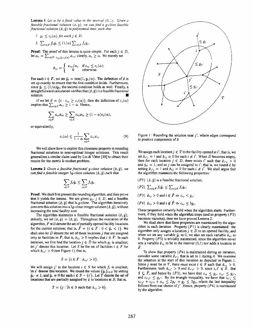
shall also let 5 denote the set of those locations j that are assignedonly to facilities in $’; that is, ~ij >0 implies that i c $’. In eachiteration, we first find the location j c D for which gj is smallest;let j’ denote this location. Let S be the set of facilities i c F forwhich t,j, >0 (see Figure 1); that is,

S={ ’iG-F:i~j, >O}.

We will aasign j’ to the location i E S for which f, is smallest;let i’ denote this location. We round the values {$i }i=s by settingji~ = 1, and Ya= Ofor each i E S – {i’}. Let T denote the set oflocations that are partially assigned by 2 to locations in S; that is,

T = {j : 3i c S such that it, > O}.

Figure 1: Rounding the sohstion near j’, where edges correspondto positive components of&

Weassign each location j E T to the facility opened at i’; that is, weset ii,, = 1 and ii, = Ofor each i # i’. When D becomes empty,then for each location j G D, there exists i’ such that i,,j > 0and y,, = 1, and so j can be assigned to i’; that is, we round i bysetting 2,,3 = 1 and tij = Ofor each i # i’. We shall argue thatthe algorithm maintains the following properties:

(P 1) (~, y) is a feasible fractional solution;

(P3) ii] >Oandi EF~c,, <g,;

(P4) iiJ >Oandi$F*Gj <3g,.

These properties certainly hold when the algorithm starts. Further-more, if they hold when the algorithm stops (and so property (P3)becomes vacuous), then we have proved Lemma 2.

We shall show that these properties are maintained by the algo-rithm in each iteration. Property (P 1) is clearly maintained: thealgorithm only assigns a location j G D to an opened facility, andwhen we set any variable ji to O,we also set each variable i,, toO. Property (P3) is trivially maintained, since the algorithm neversets a variable itj to be in the interval (0,1) nor adds a location toF.

To show that property (P4) is maintained during an iteration,consider some variable ii,2 that is set to 1 during it. We examinethe situation at the start of this iteration as depicted in Figure 1.Since j must be in T, there must exist i c S such that ii, >0.Furthermore,both i,,, > 0 and ii,,, > 0, since i, i’ c S. ButS ~ F, and hence by (P3), we have that C,l < g,, cil, < g,,,and C,/jJ < gjl. By the triangle inequality, we have that ci12 <c,~jl + Cjt, + c,, < 2gj~ + gj < 3gj, where the last inequalityfollows from our choice of j’, Hence, property (P4) is maintainedby the algorithm.

267

To show that (P2) is maintained, we note that

where the inequality follows from the fact that

E i,,=1,*ES

and that the minimum of a set of numbers is never more thantheir weighted average. Finally, ~ij < yi, and so we have thatf,, < ~i=~ fij,. But this inequality implies that the facility costof j never increases throughout the execution of the algorithm,which proves that (P2) is maintained.

Finally, we note that the simpIe rounding performed when ~is empty also maintains these four properties. This completes theproof of the lemma. ■

If we start with a feasible fractional solution (z, y) and applyLemma I to get (~, j), and then apply Lemma 2 to (i, y), theresulting feasible integer solution (2, j) has facility cost at most

On the other hand, for each location j E D, its unit assignment costin; is at most 3gj < 3cj(a) < ~ ~,EF cajzaj. BYcombining

these two bounds, we see that the total cost of (i, j)

(lo)

(11)

— ..icF ,GF JGD

If we set Q = 1/4, then we see that the total cost of (2, j) is withina factor of 4 of the cost of (z, y). By rounding an optimal solution(z, y) to the linear relaxation, we get the following theorem.

Theorem 3 For themetricuncapacitatedfacili~ Iocationpmblem,jiltering and roundingyields a 4-approximationalgorithm

In Section 5, we will give an algorithm with a somewhat betterperformance guarantee, by refining this analysis. Nonetheless, wedo not know very much about the extent to which there is an in-herent gap between integer and tractional optimal solutions to thisformulation for the metric incapacitated location problem.

3 The capacitated facility location problem

h this section, we consider the case in which each open facility canbe assigned to serve a total demand that is at most u, where u is apositive integer. We will show how to adapt our algorithm for theincapacitated case to this more general setting.

In the incapacitated case, if we are given the optimal value ofg, then it is trivial to find the corresponding z: we simply assigneach location j E D to the location i for which c~j is the minimumamong all possibilities where y, = 1. In the capacitated case, thesituation is somewhat more complicated. First of all, there aretwo variants of the problem, depending on whether each location’sdemand must be assigned to only one facility, or the demand maybefractionally split among more than one (completely) open facility.

We will first focus on the latter case. If we are given the optimalvalue of y, the problem of finding a minimum-cost assignment thatsatisfies each location’s demand, while assibaing at most u to eachopen facility is an instance of the transportation problem. (Fora review of the basics for this problem see, e.g., the textbook ofLawler [17].) Briefly, the optimal solution to this problem can befound in polynomial time, and if u and the demands d,, j E D,are integers, then the tlow values dl X,j in the solution found arealso integral. For example, this implies that in the case that thedemands are all 1and u is an integer, there is no distinction betweenthe two capacitated variants mentioned above: we always find anassignment that routes each demand to a unique open facility.

Our algorithm is based on rounding an optimal solution to itslinear programming relaxation. This linear programming relaxationis identical to the one used in the incapacitated case, except we mustexplicitly require that

O<y, <l, for each i G F, (13)

and we must impose capacity constraints

x djx,j < Uyt, for each i E F. (14)JCD

It is not possible to design an approximation algorithm for thecapacitated problem based solely on this linear programming relax-ation, since the ratio between its integer and fractional optimal isunbounded. To see this, consider an instance with u + 1 locationswith unit demands that are all distance Ofrom each other with fixedcosts jl = Oand fi = 1, i = 2, ..., u + 1. There is the followingfractional solution: set yl = 1, yz = l/u, ZIJ = u/(u + 1) andxl, = I/(u+ l), j = 1,. ... u+ 1. Thecost ofthis solution is1/u, whereas the optimal integer solution has cost 1. However,if we also allow the near-optimal solution to slightly overuse anyfacility then clearly one can, at least in this instance, find an integersolution of cost nearly equal to that for the optimal fractional one.

Motivated by this discussion, we shall call an algorithm for themetric capacitated facility location problem a (p, p’)-approximationalgon”thmif it finds, in polynomial time, a solution of total costwithin a factor of p of the true optimum, but each facility i cF is expanded to have capacity p,u at a cost of p,f, for somep, E [1,p’]. In this section, we present a (7, 7/2)-approximationalgorithm. We will express the relaxation in the capacity constraintby allowing O $ vi < p’, for each i E F. If (z, g) is a feasiblefractional solutlon to this modified linear program, then it is p’-relaxed. Furthermore, the analogue of an integer solution with thisrelaxation is that yi is either O or at least 1, for each i s F; if(z, y) is a p’-relaxed solution with this additional property, then wewill call it a p’-mloxed integer solution (even though it is not reallyinteger at all).

Once again, our algorithm is based on first filtering, and thenrounding. It is quite straightforward to generalize Lemma 1 toobtain the foIlowing result.

Lemma 4 Let CYbe a fixed value in the interval (O, 1). Given ajim.siblefractional solution (x, y), we can~nd a g-close fractionalsolution (5, j) inpolynomial time,such that

1. g, ~ cj(a),for each j 6 D;

2 z,~~fl~l ~ (l/a)z,~Ffty~;

3. (~, j) is 1/a-relaxed. ■

On the other hand, the rounding algorithm becomes a bit morecomplicated, since the incapacitated algorithm takes great advan-tage of the fact that there are no capacities: all demand fractionallyrouted to any location in S ends up being assigned to j’ (using thenotation in the proof of Lemma 2). We next prove the followinganalogue of Lemma 2.

268

Lemma 5 Givena p’-relaxedjiractionalg-close solution (5, y), wecarrjinda 2p’ -relaxedinteger3g-close solution (~, y) inpolynomialtime,such ~hat

,GF ,GF

Proofi We first describe the rounding algorithm in detail, and thenprove that it produces the claimed solution. As in the incapacitatedcase, we maintain a solution (i, y) and the algorithm graduallyrounds each O < y, < 1to either Oor 1; initially, we set & = i, weset j, = 1 for each i such that y, E [1/2, I), and we set j, = j,otherwise. We also maintain a set F ~ F of facilities i for whichO< j, < 1 (but due to the previous step, this will be equivalent torestricting O < y, < 1/2). For each j E D, the algorithm keepstrack of the fractjon of the demand for location j that is satisfiedby locations in F: let p~ = ~,=F i,, for each j E D. In this

case, we let D G D be the set of locations j for which 83 > 1/2.(In the incapacitated case, the restriction for D was, in effect that~, = 1.)

In each iteration, we first select the location j e D for whichgj is minim~, and let j’ denote this location -Again>we let

and‘T={j GD:Zli GSsuchthat&, >O}.

We do not open just one facility in S, but open the cheapest[X, S il facilities in S instead let O denote his set of facil-ities.%or each i G O, we update j, = 1, and for each i E S -0,we update j, = O. (Thus, F wilI be reset to F – S in the nextiteration.)

For each location j ~ T, there is a total demand d, currentlyassigned to locations in S, where

this demand will be rerouted to go only to those facilities in O.The problem of assigning the demand d, at each location j E T tofacilities in O, each of which is capable of handling total demandat most u, is an instance of the hansportation problem (analogousto the discussion at the beginning of this section). Our analysiswill show that any feasible solution suffices; however, it is naturalto exploit the fact that a minimum-cost solution can be found inpolynomial time. For each i E O, j ~ T, let Z,j be the amountof j‘s demand that is assigned to i by an optimal solution to thisinstance of the transportation problem. We update our solution byresetting x,, = zi, /dj for each i 60, j G T, and Xij = Ofor eachi 6 S – O, ~ E D. (All other components of ~ remain unchanged.)

When D becomes empty, we have satisfied at least half of thedemand for each location j ~ D, by assigning it to locations forwhich the component of y is at least 1. To compute the solutionclaimed by the lemma, we will simply ignore the ~j fraction of j‘sdemand that is still assigned to the remaining facilities in F, andrescale the part of i specifying the assignment to facilities not inF. That is, for each i @F, we reset y, to be 2@,,and reset iaj tobe ~iJ/(l – @j) for each j ~ D. For each i E F, we set j, = Oand set iii = O,for each j ~ D.

The proof that this algorithm delivers a suitable solution followsthe same outline as the proof of Lemma 2. We show that until thepoint at which D becomes empty, the algorithm maintains invariants

(Pi’) (i, j) is a p’-rehixed solution;

as well as (P3) and (P4),Of course, we must also show that the algorithm is well-defined.

In each iteration, we rely on an optimal solution to an auxiliary inputto the transportation problem, and so we must show that a feasiblesolution exists to this input. An input to the transportation problemhas a feasible solution provided that the total demand is no morethan the total supply. That is, we must show that the total demandfor T, ~)e~ d,, is not more than the total supply for 0, ]Olu. But

since the solution (i, y) maintained by the algorithm is a p’-relaxedsolution, we have that (2, j) satisfies the inequality

and hence

jET ICT aGS ics

Hence, the algorithm is well-defined. Furthermore, it is clear thatthis solution of the transportation problem is precisely what is re-quired to maintain the fact that (2, j) remains a p’-relaxed solution.Hence, property (.PI’ ) is maintained.

As in the incapacitated case, property (P3 ) is trivially main-tained, since the algorithm never sets ~,, > 0 while maintainingi E F. The proof for property (P4) is identical to its proof in theincapacitated case: for each z c S and j G T, c,, < 3gj.

It remains only to prove that property (P2’ ) is maintained bythe algorithm. This property is true initially, since the only locationsi # # either have y, = j,, or else j, z I/2 and y, = 1, and hencej; s 29,. Next consider the set of Ioeations S removed from j insome iteration. At the end of this iteration, we will set j, = I foreach i c O, and j, = Ofor each i E S – O. Until this iteration, foreach z E S, we have not changed j,, and hence, j, = j,. Thus, toprove that property (P2’ ) is maintained by this iteration, it sufficesto show that the inequality

~f,<2~f,y, (15)

iEO iES

holds for the value of j at the start of this iteration.Observe that since O was selected in order of cheapest fixed

costs, we have that

(16)

provided O s z, s 1, for each i E S, and ~,cs Zi = 101. If weset

IolZi=ji. —

2,s Y*‘for each z G S, (17)

then c]early ~i<s z, = 101. Since i G F, y, < 1/2. Furthermore,

j’ E D implies that

i6F KS

Since itj) s ji, we can conclude that

269

and so z, < 1, for each i E S. By combining (16), (17), and (18).we see that

and so (15) holds; property (P2’ ) is maintained.Next consider the situation when when ~ becomes empty. At

this point, property (P 1‘) implies that j, S p’, for each i E F.Since we now multiply y by at most 2, and we have ensured thatthere does not exist some y, E (O, 1), we see that the solutionis a 2p’-relaxed integer solution. Furthermore, since before y ismultiplied by 2, we know that (P2’ ) holds, then the final solutionj must have facility cost at most 4 times the cost of j, and thiscompletes the proof of the lemma. ■

Next we show how to combine Lemmas 4 and 5 to obtain a(7, 7/2)-approximation algorithm for the capacitated facility loca-tion problem. Let (z, y) denote an optimal solution to the linearrelaxation of the capacitated facility location problem. We applyLemma4 to (z, y), to obtain a 1/o-relaxed solution (z, j), and thenapply Lemma 5 to yield the 2/cwrelaxed integer solution (t, j). Foreach i E F with j, > 0, we open a facility of capacity ~i~ andassign to it a fraction &j of the demand dj at location j. The facili&cost of this solution is at most

Furthermore, the total assignment cost is at most

—

(19)

Hence, we have found a solution of total cost at most

If we set cr = 4/7, then we see that the total cost of the solutionfound is within a factor of 7 of the cost of the optimal solution tothe linear relaxation. Since the solution is 2/~-relaxed, we obtainthe following theorem.

Theorem 6 For the metric capacitatedfacility location prvblem,filtering and mundingyielak a (7, 7/2)-approximation algorithm.

Next we turn our attention to the model in which the entiredemand of each location must be assigned to the same facility.We shall call this problem the metric capacitated location pmb-Iem withunsplittable~ows. We will show that the solution foundby algorithm of Theorem 6 can be adjusted to satisfy this morestringent condition, while only slightly increasing the performanceguarantees.

The extension to the model with unsplittable flows is based ona rounding theorem of Sbmoys & Tardos [24] for the generalizedassignment problem. This theorem can be explained as follows.Suppose that there is a collection of jobs J, each of which is to beassigned to exactly one machine among the set h4; if job j ~ J isassigned to machine i c M, then it requires P;j units of processing,and incurs a cost rij. Each machine i E M can be assigned jobs

that require a total of at most P, units of processing on it, and thetotal cost of the assignment must be at most R, where R and P,,for each i E &f, are given as part of the input, The aim is to decideif there is a feasible assignment. If there is such an assignment,then there must also be a feasible solution to the following linearprogram, where Z,j is the relaxation of a 0-1 variable that indicateswhether job j is assigned to machine i:

zpZjx%j ~ Pi, for each i E M; (22)IGJ

(23)SCM jGJ

X*, > 0, for each i EM, j c J. (24)

Shmoys and Tardos [24] show that any feasible solution z can berounded, in polynomial time, to an integer solution that is feasibleif the right-hand side of (22) is relaxed to P, + maxj= J Pij.

We show next how to apply this rounding theorem to producea solution for the capacitated version with unsplittable flows. Con-sider the algorithm of Theorem 6 without specifying the choice ofa. Suppose that we apply the algorithm starting with an optimalsolution (z, ~) to the linear relaxation of the capacitated facilitylocation problem (that is, the linear program given by(1), (2), (3),(6), (13), and (14).) The algorithm delivers a 2/et-relaxed integersolution (i, j), where the facility cost and the assignment cost are,respectively, within a factor of 4/a and 3/(1 – o) of the analogouscosts for (z, y). Let O denote the set of facilities opened by thesolution (i, j); that is,

Wecan view each facility i 60 as a machine of processing capacityj,u, and each location j E D as ajob that requires a total of dj unitsof processing (independent of the machine to which it is assigned)and incurs a cost djci j when assigned to machine i. Therefore, ifweset M= O, J= D, Pi=Yiu foreachi6M,

as well as pij = dj and r,, = djc%~for each i 6 M, j E J, then iis a feasible solution to the linear program(21 )-(24).

The rounding theorem for the generalized assignment problemimplies that we can round 2 into an integer solution i such that eachfacility i E 0 is assigned a total demand at most P, + maxj ● D djand the assignment cost of this solution is

where the last inequality follows from (20). Note that, in orderfor there to exist a feasible solution with unsplittable flows, thedemand d, must be at most u, for each j c D; hence, we assumethat our instance has this property. Wecan conclude that the roundedsolution i assigns a total demand to each facility i c O that is atmost

maxdj + y,u ~ (1 + j.)u.jED

Hence, if we consider the solution (5, j) where j, = y, + 1, foreach i E O and ji = j; otherwise, then we see that it is a 1+ 2/cr-relaxed integer solution, Finally, since y, ~ 2 for each i c O(due to the final doubling when D becomes empty), we see that

270

j. < (3/2 )rjt, for each i c D, This implies that the facility cost of(i, j) is

%EF ,EF ,cF

where the last inequality follows from (19). Thus, if we comparethe solution (i, j) to tire optimal fractional solution (s, y) fromwhich we statted, we have shown that the facility cost increases byat most a factor of 6/cY, and the assignment cost increases by atmost a factor of 3/(1 – a). If we set a = 2/3, then both of thesebounds are equal to 9, and so we obtain the following theorem.

Theorem 7 For the mem”ccapacitatedfacility location problemwith unsplittableflows, )lten”ng and rounding yields a (9, 4)-appro-ximationalgon”thm.

Khuller & Sussmann [15] have introduced the notion that onecan open multiple facilities of capacity u at each location (in thecontext of the capacitated k-center problem), We can also obtainanalogues of Theorems 6 and 7 for this variant of the capacitatedfacility location problem. In other words, we are now interestedin obtaining solutions in which each Vi is an integer. We start bysolving the linear relaxation, which is identical to the one usedabove, except that we replace (13) with just vi z O, for eachz G F. Lemma 4 must now be modified to reflect that we obtaina solution (5, j) that is feasible for the new linear relaxation, butstill has the property that j, < ( 1/cx)y., for each i c F; otherwiseLemma 4 remains unaffected. The statement of Lemma 5 mustalso be modified; we now require that (2, j) be a feasible fractionalsolution, and that the solution (i, j) be such that each j;, z c F,is an integer. This apparently stronger claim can be obtained byessential y the same proof. The only modification needed is in theinitialization of j: at the start of the algorithm, we set yi = [j,l foreach i such that jj ~ 1/2, and as before, we set j; = j; for each isuch that j, < 1/2, This also maintains propetty (P2’ ), since thisinitial rounding increases the cost incurred for each facility locationz ~ F by at most a factor of 2. Of course, we no longer need tomaintain property (P 1‘). By using these modified lemmas, we canobtain the following analogue of Theorems 6 and 7.

Theorem 8 For the mem”c capacitatedfacili~ location problemwith multiple facilities allowed, filten’ng and rounding yields a 7-appmximation algon’thm with splittablejlows, and a 9-approx-imationa[gon”thmwithunsplittable~ows.

Since the performance guarantees have not become worse byimposing this additional restriction that the capacity used for eachlocation is an integer multiple of u, one might wonder why we havenot stated Theorems 6 and 7 in this stronger way. The reason is thatby maintaining this integerized capacity, we do need to introduce agreater relaxation of the capacity bound. For example, in Theorem6 we would produce a 2[$1 -relaxed solution, rather than simply a2p’-relaxed solution.

4 The 2-level imcapackated facility location problem

Another more general version of the facility location problems thatwe consider is the setting in which there is a 2-level hierarchyof facilities. Such 2-level facility location problems have beenconsidered extensively in the literature (see, for example, [1, 14,27, 28]).

We shallonly consider the 2-level version of the incapacitatedproblem, but it is possible to obtain similar extensions for the capac-itated models as well. In the 2-level incapacitated facility locationproblem, there is, as before, a set of demand points D, and a set of

locations F where hub facilities can be built. However, each unitof demand at a point in D must now be shipped from a hub facilityvia an intermediate transit station; let E denote the set of locationsat which one of these transit stations may be built, We shall con-sider the metric case in which the unit cost of shipping between twolocations i,.j c D U E U F is equal to C,j; that is, these costs arenon-negative, symmetric, and satisfy the triangle inequality, and sofor any i, j,k 6 D UEUF, C,l +c,k > C,k, Each location k G Dhas a specified demand dk. For each i c F, the cost of buildinga hub facility at location i is f, and for each j ~ E, the cost ofbuilding a transit station at location j is e~. Each unit of demand atlocation k c D must be shipped from some location i G Fat whicha hub is built via a location j G E at which a transit station is built,incurring a shipping cost of C,2+ c, k. We shall let C,Jk denote theshipping cost ci~ + c, k. The aim is to determine which hubs andtransit stations to build so that the total building and shipping costis minimized. We will show how to extend Theorem 3 to obtain a4-approximation algorithm for this more general model.

First, we give a linear programming relaxation of the 2-levelincapacitated facility location problem. All of the variables in thislinear program are relaxations of 0-1 decision variables, and thereare three types of variables: the variables Xijk, ~ G F, j 6 E,k < D, indicate whether the demand at location k is routed througha transit station at location j from a hub facility at location i; thevariables vi, i c F, indicate if a hub facility is opened at locationi; and the variables z,, j 6 E indicate if a transit station is openedat location j.

subject to

for each k G D, (26)

for each i E F, k E D, (27)

for each j 6 E, k c D, (28)

for each i c F, j E E, k E D, (29)

for each i E F, (30)

for each j c E. (31)

As in the single-level setting, we will show that any feasiblesolution to the linear relaxation of this integer program can berounded to an integer solution that has objective function valueat most 4 times as much. This rounding algorithm will closelyresemble the algorithm used to prove Theorem 3. We first modifithe definition ofg-close. A feasible solution (z, y, z) to this linearrelaxation is said to be g-close if it satisfies the property

xijk >O*~]k <gk. (32)

We shall also modi~ the notion of an a-point. For each locationk E D, we sort the costs c,,k over all pairs i G ~, j E E, innondecreasing order; if we add the associated values z,, k in thissorted order, then we let ck (a ) be the cost associated with the firstpair for which this running sum is at least a. It is straightforwardto obtain the following extension of Lemma 1.

Lemma 9 Let a be a fixed value in the interval (O, 1). Given afeasible f?actional solution (z, g, z), we canflnd a g-close fiasiblefractional solution (s, ~, 2) inpolynomial time,such that

271

for each k E D,

■

(33)..

tGF 3GE

Next we prove the following analogue of Lemma 2.

Lemma 10 Given a feasible fractional g-close solution (~, ~, 2),we canfind afeasible integer3g-cIose solution (i, ~, .2)such that

,GF ,cE ,EF ,cE

Proofi We shall first give the rounding algorithm, and then provethat the solution found has the properties claimed by the lemma. Thealgorithm is quite similar to the one used in the single-level inca-pacitated case. We maintain a feasible fractional solution (i, j, 2)that is initialized to (5, ~, 2). We will maintain a collection R oftriples (i)j, k), i c F, j ~ E, k E D, that have been rounded tohave ~,~k = 1 (and hence ~, = ~j = 1). Initially, R = o (evgn ifsome components of i are equal to l). We also maintain a set D oflocations k c D that do not participate in any triple in R; that is,

D={i ED:(2,j, k) CR Si #k}.

In each iteration, we first find the location k E b for which gkis smallest; let k‘ denote this location. Let S denote the set of pairs(i,j ) that are used to supply k’ in the cument solution; that is,

S = {(i, j) : ~t,kf > 0}.

We also introduce notation for those locations that occur in somepair in S; let

SF = {i 6 ~ : ~j such thatz,j~l > O}

andSE = {j E E : ~i such that xljkl > O}.

We will assign k’ to be served by the facility-transit station pair(i, j) G S for which j, + .1 is smallest; let (i’, j’) denote thispair. We round the values {ji }i~s~ by setting ji~ = 1, and j; = Ofor each i E SF – {z’}. Similarly, we round {~i }~cSE by setting~j, = 1, and ~j = O for each j c SE – {j’}. Let T denote theset of locations that are partially assigned by t to use locations ineither SE or SF; that is,

T={k~fi:3~i,~ >Osuchthati CSForj ESE}.

We assign each location k E 2’ to the facility opened at i’ throughthe transit station located at j’; that is, for each k s T, we reset~t~j,k = 1 and ~:~~ = Ofor each (i, j) # (i’, j’); furthermore, weadd (i’, j’, k) to R. When D becomes empty, then for each locationk c D, there exists (i’, j’) such that ii,j,b = 1, and so we havecomputed an integer solution.

We shall argue that the algorithm maintains the following prop-erties:

(P{ ) (2, j, 2) is a feasible fractional solution;

(P2) ~,,~ fiYi + E,CE ej& 5 E,CF fi$i + xj~~ %Z;

(P3) X,,k > Oand (i, j,k) @ R a c,, k < gk:

(P4) x,,, > Oand (i, j,k) c R * c,,, s ~gk;

(P5) (i,j, k) c Rand 2t,~ >0 ~ (i, j,~) c R;

(P6) (i,j, k) ● R ~ (~,j~ = Oforeachj # j, k E D and

~ijk =Oforeachi# i, i G D.)

These properties certainly hold when the algorithm starts. Further-more, if they hold when the algorithm stops (and so property (P3)becomes vacuous), then we have proved Lemma 10. The proofthat (P 1) is maintained is similar to the proof of property (P 1) inLemma 2: the main observation is that whenever some j, or 22 isset to O,we also set all corresponding variables ~,$k to O.

The new properties (P5) and (P6) are straightforward conse-quences of the way in which the rounding algorithm proceeds. Toprove (P5), consider two triples (i, j, k) and (i, j, k) for which~~jk >0 and ilj~ >0 at the start of the algorithm. If either tripleis placed in R, then in the same iteration, the algorithm will putthe other one in R as well. Since the algorithm never changes acomponent of i from being Oto being positive, this implies thatproperty (P5) holds.

Toprove (P6), consider two triples (i, j, k) and (i, j, i), wherej # j, for which initially we have that ~,jk >0 and Xtjk >0. Ifeither of these triples is added to R, then in the same iteration, wemust also set the variable corresponding to the other triple to O; inother words, if (i, j, k) c R, then iijk = O, and so the first halfof (P6) has been proved. The proof of the second half is exactlyanalogous.

The proof that property (P4) is maintained is similar to theproof given for (P4) in Lemma 2. Consider some variable ;, IJ,kthat is set to 1 during some iteration of the algorithm. However,this implies that k 6 T, since the algorithm only sets to I thosecomponents of ~ for which the last index is in T. For the locationk’ used in this iteration (that is, the location in D with minimum gkvalue), we have that ~al~lk, > O; furthermore, (i’, j’, k’) was notin R at the start of this iteration, and hence, by (P3), G,,,k) < gkl.Since k G T, we know that there exists ~;~k >0 such that i 6 SFor j E SE. We shall consider these two cases separately.

Case 1: i E SF. It follows from i c SF that there existsj E -E such that that ~tjk, > 0. Since k’ c D, this implies that(i,~, k’) #R, and SOc,jk, ~ gk,.

We will show next that (i, j, k) @ R, and hence C,jk ~ gk.

Suppose that j # j. Since i,jk? >0, it follows ftom (P6) that(i, j, k) @ R. On the other hand, suppose that j = j, Since

k’ G D,weknowthat (i,j, k’) @R,andhence, by(P5), (i, j,k) =(i, j, k) # R.

We wish to show that Ci,j,k ~ 3gk. However, by the triangleinequality, we can bound c,,j, k by the total cost of the path ffom i’to j’ to k’, followed by the path from k’ to j to i, followed by thepath from i to j to k. Hence,

c%,l,k~ ca,,,k, + c,ik, + c,, k s gkt +gkl +gk s qgk.

Case 2: j E SE. Since j E SE, there exists i such thati~jkl >0. Again, since k’ E D, we know that (i, j, k’) @ R, andhence ci,kl < gkl

We will show next that (i, j, k) @ R, ~d hence cijk < gk.Suppose that i # i. Since ~ijk, >0, it follows from (P6) that(i, j, k) @R. On theotherhand, suppose that i = i. Since k’ c D,we know that (i, j, k’) = (i, j, k’) ~ R, and hence, by (P5),(i, j, k) @R. Finally, we can bound cl, ,,k by the cost of the pathfrom i’ to j’ to k’ followed by the edge from k’ to j, followed bythe edge from j to k. Hence,

ci,~~k~ ca,j,k, + cf,k, + ~~k s gkt + gk) +gk ~ qgk,

272

and we have shown that properry (P4) is maintamed.To show that (P?) is maintamed, we note that

where the inequality follows from the fact that the minimum ofa set is no more than any convex combination of it. Finally.

and

(.>j)cs l~sE z:(t,, )es l~sE

Hence

But this inequality implies that the total of the facility cost and transitstation cost of (~, 2) never increases throughout the execution of thealgorithm, which proves that (P2) is maintained. This completesthe proof of the lemma. ■

By combining Lemmas 9 and 10 in a manner identical to theway in which Lemmas 1 and 2 were used to prove Theorem 3, weobtain the following theorem.

Theorem 11 For the 2-level incapacitated facilip location prob-lem, fikering and rounding yieIds a 4-approximation algorithm.

5 A randomized filtering algorithm

In this section, we will show that by choosing the threshold a atrandom, we are able to obtain improved performance guarantees. Infact, it will also be straightforward to derandomize these algorithms.This use of randomization is very much in the same spirit as therandomization used in scheduling algorithms by Chekun, Motwani,Natarajan, & Stein [4] and Goemans [9].

For each of the facility location models that we have discussedin the previous three sections, we have given an approximationalgorithm based on a particular choice of Q, but it is evident thatwe can also consider the algorithm for any choice of a E (O, 1).For each model, the randomized algorithm is quite easy to state:we choose a uniformly in the interval (~, 1), where ~ will befixed later to optimize the algorithm’s performance; then we applythe deterministic algorithm with that value of a. Tbe intuitionfor cutting off the uniform distribution at some point/3 is that thefiltering step increases the facility cost by a factor of 1/a, and sowe will need to bound E[l/cY].

We first analyze this approach for the incapacitated (single-level) facility location problem. At the core of our analyses is thefollowing simple lemma about the a-point of a cost fimction, whichwas first observed by Goemans [8]. Goemans used this observationto show that if one implements the cwpoint 1-machine schedulingalgorithm of Hail, Shmoys, & Wein [11]where a G (O, 1) is chosenwith probability density function ~(a) = 2a, then its performanceguarantee improves from 4 to 2 (which had already been shown in[IO] by a less direct approach). Independent of our work, Schulz&Skutella [23] also used this observation for improved performanceguarantees for other scheduling models.

Proof For simplicity of notation, let us assume that

CI, <c?,<.. .<cn, ;that is, the permutation n is the identity. The function cl (o) is a stepfunction, which can be described as follows. Let i, <22 <...< itbe the indices i for which ~i, >0. The function c, (et) is equalto c,,, for each a in the interval (~~~~ z,,j,~~=l z,,~]. ‘Wewish to compute the area under this curve; for the interval from

x::; u., toz:=, z,,,,this area is exactly c,k~ . z,~j. Hencethe total area is exactly

which proves the lemma. ■

Weshow next how to apply this lemma. In fact, we have alreadyproved that the filtering and rounding algorithm of Theorem 3 findsa solution of cost at most ~ ~ ,~~.f1Y1+3zj6~ d,c,(~) for anygiven cz(see equation (11)). Hence, we see that the expected costof the solution found by the randomized algorithm is

Hence, we wish to choose ~ so as to minimize max{ w, ~ };

that is, we set ~ = 1/e3, to yield the following theorem.

Theorem 13 For the metric uncapacitatedfacili~ location pro-blem,randomizedjiltenng and rounding yields an algorithm thatfords a solution whose expected total cost is within a factor of3/(1 – e-3) <3.16 of theoptimum.

One reinterpretation of the proof of this theorem is that for ~selected at random in this manner, we have

where p = ~l_~_3). Of course, a consequence of this is that there

must exist a choice for ct for which this function is not greaterthan its expectation. Thus, if we can find the a = a“ for which

A ~.c~ f~yi + 3 ~lGD ~j%(~) is minimized> then@ runningthe deterministic filtering and rounding algorithm with a = a“, weare assured of finding a solution within the expected performanceguarantee. Fortunately, the step function nature of cj (a) makes thisa particularly simple function to minimize; we need only check allbreakpoints of all of the step functions cj (a), j G D. This yieldsthe following theorem.

Theorem 14 For the metric incapacitated facili~ location pmb-Iem,-filteringand roundingyields a 3.16-appmximation algorithm.

273

The same randomization and derandomization technique can beapplied to each of the theorems in this paper, yielding somewhatimproved constants for each of the performance guarantees. Inthe capacitated case, for example, if we again choose a uniformlywithin the interval between [f?,1] (where P will be chosen later),then the expected total cost of the solution found by the algorithmis at most

where (z, y) is the optimal solution to the linear relaxation of thecapacitated facility location problem. If we set fl = e–3/4, then wesee that the expected cost is within a factor of 3/(1 – e-314) <5.69of the cost of the linear relaxation optimum (z, y). The solution(2, j) found by the algorithm is also guaranteed to be 2/a-relaxed,and so the expectation of the maximum capacity used at any fa-cility is at most 2u13[l /0] < ~(l_~--Sf4) M s 2.85u. When we

derandomize this algorithm, by focusing on the optimal choice ofa with respect to the bound on the cost of the solution, we cannotsimultaneously keep the guarantee for the maximum capacity usedclose to its expectation, 2.S5U. However, we are choosing a within

–~1~ 1 and tie bound 2/~ is at most 2e3’4 5 4.24the interval [e , ],throughout this interval. Hence, we obtain the following theorem.

Theorem 15 For themem’c capacitatedfaciIity location problem,~kering and rounding yields a (5.69, 4.24)-approximation algo-rithm.

The same approach can be applied to each of the theorems in thispaper. In particular, for Theorem 7, the performance guarantee of(9,4) canbeirnprovedto (3/(1 -e-’\ 2), l+2e’f2) ~ (7.62,4.29);for Theorem 8, the performance guarantees of 7 and 9 can beimproved to 5.69 and 7.62, respectively; and for Theorem 11, theperformance guarantee of 4 can be improved to 3.16.

Acknowledgments Weare grateful to Michel Goemans for shar-ing with us his randomized analysis of the 1-machine schedulingalgorithm of [11], since this ultimately led to the results in Section<J.

References

[1] K. Aardal, M. Labb4, J. Leung, and M. Queyranne. On thetwo-level incapacitated facility location problem. INFORMSJ. Compul., 8:28%301, 1996.

[2] M. L. Balinksi. On finding integer solutions to linear pro-grams. In Proceedings of theIBM Scien@c ComputingSym-posium on Combinatorial Pivblems, pages 225-248. IBM,1966.

[3] J,Bar-IIan,G. Kortsarz,andD. Peleg. How to allocatenetworkcenters.J. of Algorithms, 15:385-415, 1993.

[4] C. Chekuri, R. Motwani, B. Natarajan, and C. Stein. Approx-imation techniques for average completion time scheduling.In Proceedings of the 8th Annual ACM-SIAM SymposiumonDiscreteAlgorithms,pages 609-618, 1997.

[5] G. Comu4jols, M. L. Fisher, and G. L. Nemhauser. Locationof bank accounts to optimize float: An analytic study of exactand approximate algorithms. ManagementSci., 8:789-810,1977.

[6] G. Comuejols, G. L. Nemhauser, and L. A. Wolsey. Theincapacitated facility location problem. In P. Mirchandaniand R. Francis, editors, DiscreteLocation Theory,pages 11!+171. John Wiley and Sons, Inc., New York, 1990.

[7] M, E, Dyer and A. M. Frieze. A simple heuristic for thep-center problem, Oper Res. Left.,3:28$288, 1985.

[8] M. X. Goemans. Personal communication, 1996,[9] M. X, Goemans. Improved approximation algorithms for

scheduling with release dates. In Proceedings o~~he 8thAn-nual ACM-SIAM Symposiumon Discrete Algon”thms,pages591–598, 1997.

[10] L, A. Hall, A. S. Schulz, D, B. Sbmoys, and J. Wein, Schedul-ing to minimize the average completion time: on-line andoff-line approximation algorithms. 1996. Submitted to Math,Oper Res.

[11] L. A. Hall, D. B. Shmoys, and J. Wein. Scheduling to minimizethe average completion time: on-line and off-line algorithms.In Proceedings of the 7thAnnual ACM-SIAM SymposiumonDiscreteAlgon’thms,pages 142–151, 1996.

[12] D. S. Hochbaum, Heuristics for the fixed cost median problem.Math. Programming, 22:148-162, 1982.

[13] D. S. Hochbaum and D. B. Shmoys. A best possible approxi-mation algorithm for the k-center problem. Math. Opex Res.,10:18&184, 1985.

[14] L. Kaufman, M. vanden Eede, and P. Hansen. A plant andwarehouse location problem. Operan”onalReseamh Quar-terly,28:547–557, 1977.

[15] S. KIrtdlerand Y.J. Sussmann. The capacitated k-center prob-lem. In Proceedings of the 4th Annual European Sympo-siumon Algordhms, LectureNotesin ComputerScience 1136,pages 152–166, Berlin, 1996. Springer.

[16] A. A. Kuehn and M. J. Hamburger, A heuristic program forlocating warehouses. J4anagementSci., 9:643-666, 1963.

[17] E. L. Lawler. Combinatorial Optimization: Networks andMatmids. HoIt, Rinehart, and Winston, New York, 1976.

[18] J.-H. Lin and J. S. Vitter. Approximation algorithms for ge-ometric median problems. Inform Pmc, Lett,, 44:24$249,1992.

[19] J.-H, Lin and J. S. Vitter. e-approximations with minimumpacking constraint violation. In Proceedings of the 24th An-nual ACM Symposiumon Theo~ of Computing, pages 77l–782, 1992.

[20] A. S. Marine. Plant location under economies-of-scale-decentralization and computation. ManagementSci., 11:213-235, 1964.

[21] P. B. Mirchandani and R. L. Francis, eds. Discwte LocationTheory. John Wiley and Sons, Inc., New York, 1990.

[22] G. L. Nemhauser and L. A. Wolsey. httegerandCombinatotialOptimization.John Wiley and Sons, Inc., New York, 1988.

[23] A. S. Schulz and M. Skutella. Randomization strikes in LP-based scheduling: Improved approximations for rein-sum cri-teria. Technical Report 533/1996, Department of Mathemat-ics, Technical University of Berlin, 1996.

[24] D. B, Shmoys and E. Tardos. An improved approximationalgorithm for the generalized assignment problem. Mathe-matical Programming,62:461474, 1993,

[25] J. F. Stollsteimer. The eflec~of ~echnicalchange and outputexpansion on the optimumnumber size and location of pearmarketingfacilities in a Callfomia pear producing reg”on.PhD thesis, University of California at Berkeley, Berkeley,California, 1961.

[26] J. F. Stollsteimer. A working model for plant numbers andlocations. J. Farm Econom., 45:631-645, 1963.

[27] D. Tcha and B. Lee. A branch-and-bound algorithm for themulti-level uncapaeitated location problem. EuropeanJ, OperRes,, 18:3W13, 1984.

[28] T. J. Van Roy and D. Erlenkotter. A dual based procedure fordynamic facility location. ManagementSci., 28: 1091–1105,1982.

274