209-1

Facies Modeling in Presence of High Resolution Surface-based Reservoir Models

Kevin Zhang

Centre for Computational Geostatistics Department of Civil and Environmental Engineering

University of Alberta

A surface-based facies modeling approach is illustrated in this paper. The relative spatial position information is transformed into facies probabilities information based on user-specified facies template, which may be utilized by conventional cell-based facies modeling algorithms, such as BlockSIS and GTSIM. The large scale facies distribution is represented by the surface model, and fine scale facies distribution may be controlled by semivariograms. The spatial structures and facies distribution are reproduced. The model will lead to more accurate reservoir simulation. The workflow for surface-based facies modeling is proposed with a synthetic case study example.

Introduction

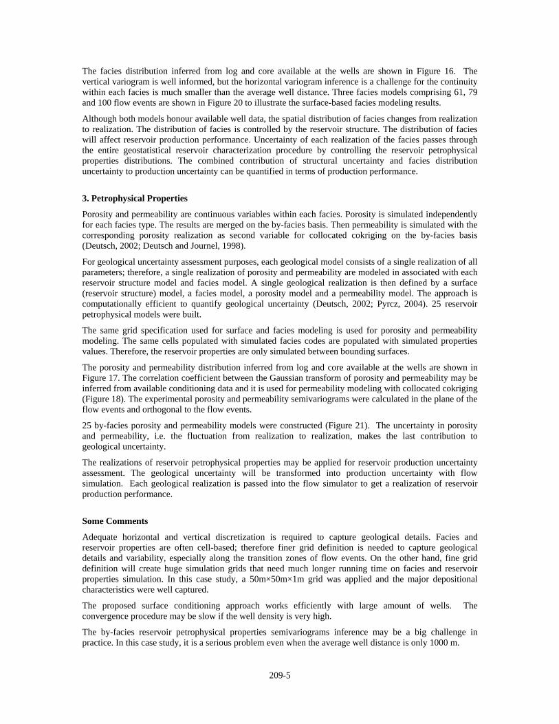
In terms of waning flow regime from bottom to top and with increasing path across a basin, turbidity current loses both energy and sediment; hence the distal turbidites, as well as deposits on the levees, do not show the complete turbidite sequences (Figure 1; Reineck and Singh, 1980). The resulting hypothetical facies plan distribution is shown in Figure 2. This is also the idealized facies distribution within a second-order turbidite lobe. The loss of energy results in progressively less basal erosion, deposition of progressively finer sediment and thickening of the finer part of the sandstone / mudstone couplet. Most importantly, accompanying the downcurrent (lateral) grading of size and bed thickness, there is a change in the internal structure of the sand component of the couplet, with progressively higher parts of the Bouma sequence forming the base of the turbidite bed (Figure 3; MacDonald, 1992). Based on above analysis, the idealized facies distribution of a second-order turbidite lobe is shown in Figure 4. Three facies are assumed in this diagram.

Facies models are often cell based. For a given cell, its depositional coordinates can be easily determined based on its vertical, longitudinal and transverse relative position within a second-order lobe. If facies trends are known, the position information may be transformed to facies proportions and taken into account in facies modeling. Therefore, surface shape information will be brought into facies modeling stage.

The vertical facies trend may be available from well logs. Areal facies trend inference is difficult due to sparsely spaced wells. Therefore, an areal facies conceptual model is used often in practice, which may come from experienced geologists. These models are problem specific and therefore no universal solutions exist. In this research, the areal facies distribution in Figure 2 is applied to illustrate the proposed methodology.

Conceptual models may also be defined analytically. There are several analytical turbidite lobe models available. One popular model is the “simple” lobe model proposed by Deutsch (2002). Assuming that the inner facies distribution follow the lobe boundary shape, the facies boundary may be expressed as:

2

4 ( - ) [ (1- )], 02 2

-1- ( ) , -

x xw W w x ll l

yx lW l x LL l

⎧ + × × < <⎪⎪= ⎨⎪ × < <⎪⎩

(1)

where x, y are the X, Y coordinates of facies boundary, w, W are the minimum and maximum facies width, l is the X position of maximum width, and L is the maximum length. An idealized areal facies distribution is shown in Figure 5.

209-2

For a given cell within a second-order lobe, its depositional coordinates may be denoted as Xr, Yr and Zr. It may have the same vertical trend as some position on the centerline. The location can be inferred under some assumptions. Therefore, the 3D facies trend calculation problem may be simplified to a 2D facies trend calculation problem. One convenient assumption is that for any point on axis, it has the same facies changing rate longitudinally and laterally (Figure 6), that is,

1 1 1

2 2 1X Y YX Y

= = (2)

where Y1 is the distance from P1 to its perpendicular projection on centerline, A; Y2 is the lateral facies width of Facies Two from A; X1 is the distance from A to P2, the position has same vertical facies trend as P1; and X2 is the longitudinal distance from A to the boundary of Facies Two.

A linear vertical facies trend model may be applied to simulate the facies change proximally according to proximity theory. For convenience, the facies trend is defined in relative scale. Since the areal lobe shape is known, only vertical trend definition is needed in facies proportion calculation. An example linear vertical trend template is shown on the left plot in Figure 7.

The calculated facies proportions may be rescaled to honour global proportions,

1 ( ) ( )Dk r k k rp z P p z= ⋅ (3)

where k denotes for the kth facies, 1 ( )Dk rp z is the updated facies proportion, kP is the global proportion,

and ( )k rp z is the calculated facies proportion.

Integration of Statistical Trends

When well spacing is close enough, areal facies trends may be inferred. In this case, both areal and vertical facies trends may be applied. For simplification, both vertical and areal facies trends are defined in relative scale. An elliptical areal facies trend and a linear vertical facies trend are applied in this research. The elliptical shape is selected because it is simple and the facies distribution follows the shape of the lobe outline very well (Figure 8). An example 2D trend template is shown in Figure 7.

Under the assumption that the areal and vertical facies trends are conditionally independent, the final facies trend may be expressed as,

( , ) ( ) ( )CIk r r k k r k rp y z P p y p z= ⋅ ⋅ (4)

where k denotes for the kth facies, ( , )CIk r rp y z is the updated facies proportion under conditional

independence assumption, kP is the global proportion, and ( )k rp y and ( )k rp z are the calculated areal and vertical facies proportions, respectively.

A common shortcoming of the conditional independence assumption is that the high values may be extremely high and low values may be extremely low (Deutsch, 2002). To overcome this drawback, the permanence ratio approach (Journel, 2002) is applied to integrate the two types of trends,

1

( , ) 1 1 ( ) 1 ( )( ) ( )

k

PR kk r r

k k r k r

k k r k r

PPp y z P p y p z

P p y p z

−

=− − −

+ ⋅

(5)

where ( , )PRk r rp y z is the updated facies proportion under permanence ratios assumption. The calculated

facies proportions are also scaled to honour global facies proportions.

209-3

Application of Facies Proportions

Programs available in the public domain to integrate calculated facies proportions include GTSIM, BlockSIS and sisim_lm. GTSIM applies facies proportions directly to truncate continuous Gaussian values to build facies model. BlockSIS and sisim_lm integrate facies proportions as secondary data.

For surface-based facies modeling, both facies types and facies proportions are known at wells, so the corresponding Gaussian values may be easily calculated by reversely transforming the centroid ccdf value of the facies (Figure 9). A Fortran 90 program, CalcSgsData, was written to perform the proposed methodology.

A comparison of above transformation approach and conventional transformation approach is shown in Figure 10. Although the transformed values do not have perfect Gaussian shape, they are consistent with the facies proportions at wells. A typical GTSIM workflow for surface-based facies modeling with facies proportions information is shown in Figure 11. The GTSIM program was modified to have the ability to read keyout array, so the volume out of the bounding surfaces will not be modeled. If a cell is located within the strata, its keyout value equals to 1; otherwise it equals to 0. An example GTSIM parameter file is shown below and each parameter is included in Table 2.

There are two algorithms that can integrate facies proportions as secondary data. One is the non-stationary simple kriging with residuals from the locally varying mean probabilities,

( ) ( ) ( ) ( ) ( )1

*

1; ; ;

nSK

LVM k ki k p k i k pα α αα

λ=

⎡ ⎤− = −⎣ ⎦∑u u u u ui (6)

Another one uses one minus the sum of the weights assigned to the local mean,

( ) ( ) ( ) ( ) ( )2

*

1 1; ; ; 1 ;

n nSK SK

LVM ki k k i k k pα α αα α

λ λ= =

⎡ ⎤= + −⎢ ⎥

⎣ ⎦∑ ∑u u u u u (7)

When locally varying mean values are smooth, the differences between Function (6) and (7) are minor (Deutsch, 2006). sisim_lm program is not recommended for it cannot utilize the keyout array; therefore, the volume above the top surface or below the base surface will be filled up with background facies.

Synthetic Case Study

The data

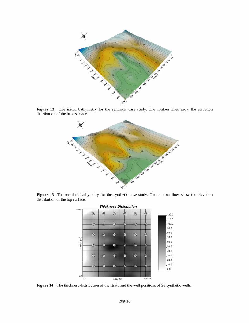
The bounding surfaces were synthetically constructed. The slope gradient is about 2 degrees, which is common in distal continental slope environment. The stratum is roughly 60m (198ft) thick and pinches out towards west and north (Figure 12 and Figure 13). The initial bathymetry is a northwest-southeast-trending submarine depression, and it is assumed that 36 vertical wells are available (Figure 14). 36 wells are chosen as a reasonable high level of conditioning in a typical deepwater reservoir study. The 36 wells are regularly distributed (1000 m). A large amount of wells are used in this case study for better variogram inference and enough well data for controlling facies, porosity and permeability distributions. The newly developed dual-spline error surface interpolation approach works efficiently with a relatively large number of wells. All available data will be honoured, including well picks, facies, porosity and permeability at wells. No large-scale seismic trend and areal trend are applied.

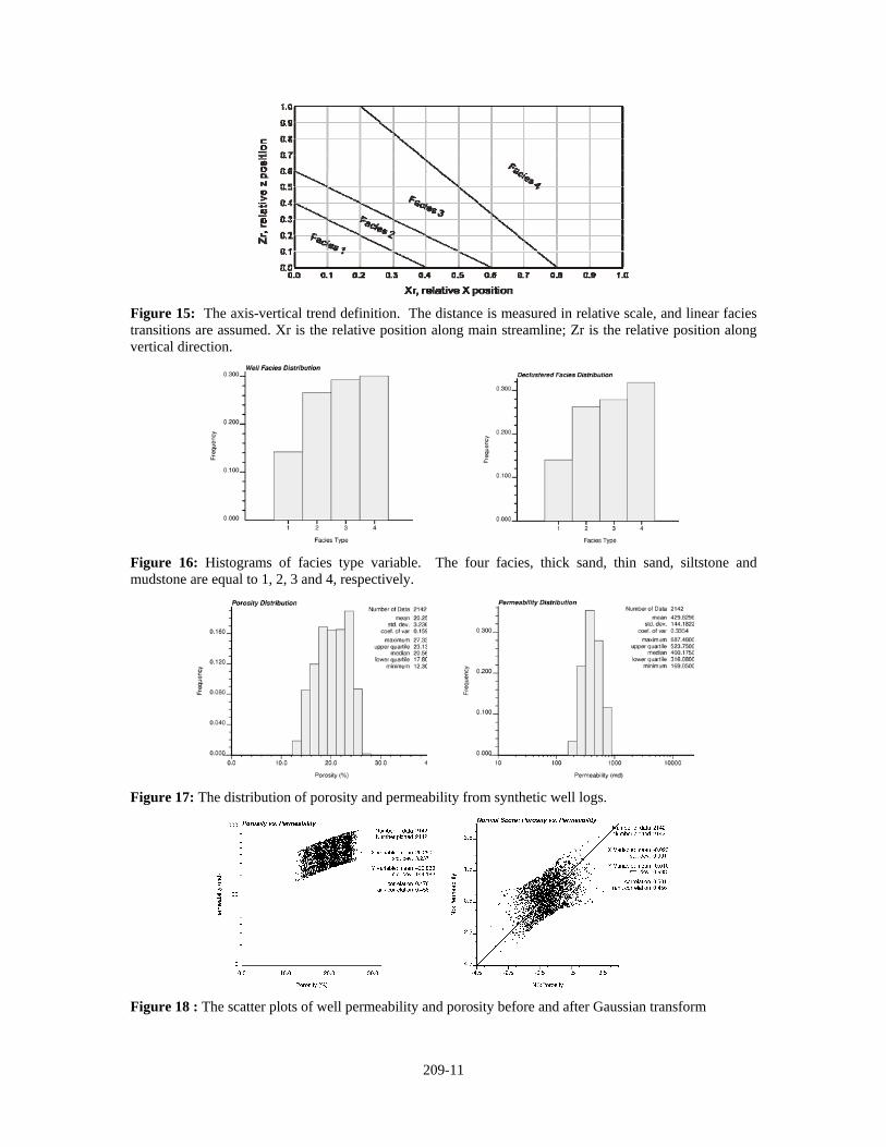
The turbidite reservoir is dominated by compensational cycles that constrain the distribution of lithofacies. Facies along wells were sampled from an unconditional SIS-based realization for modelling the facies distribution at wells. Four facies types are recognized (Table 3 and Figure 15) and linear vertical facies trend is assumed from proximal to distal based on proximality theory. Declustering technology is applied to rebuild global facies distribution (Figure 16). In this synthetic case study, the “true” facies model is assessable, so we know the “real” facies proportions.

Porosity and permeability along the wells were synthetically sampled on a by-facies basis. Permeability is commonly related to porosity. For simplicity, an experimental logarithm relationship between porosity and

209-4

permeability is applied to build the porosity-based permeability distribution (Deutsch, 2002). The regression equation takes the form:

*0 1( )log K a a φ= + ⋅ (8)

where *( )log K is the predicted logarithm of permeability, a0 and a1 are regression coefficients, and φ is porosity. The reservoir is assumed to be a mud-rich turbidite fan. Therefore, mudstone is the most important facies component under this geological background. Porosity and permeability histograms are shown in Figure 17. The scatter plots of permeability and porosity are shown in Figure 18.

Category Dominant Lithology Bedding Bouma Sequence

Facies 1 Sandstone Thick – massive, crudely graded A-division

Facies 2 Sandstone Thin – medium, subtly graded B, C-division

Facies 3 Siltstone Thinly bedded siltstone D-division

Facies 4 Mudstone Devoid of mudstone E-division

Geostatistical Work Flow

A common geostatistical workflow for surface based modeling is to model: (1) reservoir geometry that honours available wells picks based on geological concept models and related statistical information; cell-based facies proportions model will be built at the same time based on modeled surfaces distribution; (2) lithofacies considering facies proportions model as secondary data; (3) porosity distribution within each facies; and (4) permeability distribution within each facies considering porosity as a secondary variable (Deutsch, 2002; Pyrcz, 2004, 2005). These models are conditioned to all available well data and analog information.

1. Model of Reservoir Geometry

Large-scale reservoir geometry can be visualized with seismic and are known for subsequent surfaces modeling. In this case study, two source locations for the turbidite lobes are selected based on global base surface geometry. There are four facies types: graded sandstone, laminated sandstone, siltstone and mudstone (Figure 15). Mudstone has the largest proportion (Figure 16). Subsequent flow event deposits have persistent internal lithofacies trends which are defined by a linear proximal-distal facies trend template (Figure 15). An idealized areal facies distribution is assumed.

25 conditional surface models were built to demonstrate the surface-based modeling approach. Although all conditional surface models honour available well picks, the number of surfaces and spatial structures are different, which indicates that the fine-scale reservoir structure has significant uncertainty. The number of surfaces is a good indicator of spatial structure uncertainty; it changes from 61 to 100 with a lognormal shape. The median number of surfaces is 78. Three conditional surface models are shown in Figure 19 to compare different spatial structures, which comprising 61, 79 and 100 flow events, respectively.

The surface models affect reservoir production performance. This is the initial motivation of quantitative stratigraphic forward modelling (Cross and Lessenger, 1998). Each realization of the reservoir structure is passed through the entire subsequent process of geostatistical reservoir characterization.

2. Lithofacies Models

There are progressively finer sediments and thickening of the finer part of the sandstone / mudstone as the sediments go from proximal to distal direction. The trend information is integrated into cell-based facies model as facies proportions information. BlockSIS is applied in this case study.

209-5

The facies distribution inferred from log and core available at the wells are shown in Figure 16. The vertical variogram is well informed, but the horizontal variogram inference is a challenge for the continuity within each facies is much smaller than the average well distance. Three facies models comprising 61, 79 and 100 flow events are shown in Figure 20 to illustrate the surface-based facies modeling results.

Although both models honour available well data, the spatial distribution of facies changes from realization to realization. The distribution of facies is controlled by the reservoir structure. The distribution of facies will affect reservoir production performance. Uncertainty of each realization of the facies passes through the entire geostatistical reservoir characterization procedure by controlling the reservoir petrophysical properties distributions. The combined contribution of structural uncertainty and facies distribution uncertainty to production uncertainty can be quantified in terms of production performance.

3. Petrophysical Properties

Porosity and permeability are continuous variables within each facies. Porosity is simulated independently for each facies type. The results are merged on the by-facies basis. Then permeability is simulated with the corresponding porosity realization as second variable for collocated cokriging on the by-facies basis (Deutsch, 2002; Deutsch and Journel, 1998).

For geological uncertainty assessment purposes, each geological model consists of a single realization of all parameters; therefore, a single realization of porosity and permeability are modeled in associated with each reservoir structure model and facies model. A single geological realization is then defined by a surface (reservoir structure) model, a facies model, a porosity model and a permeability model. The approach is computationally efficient to quantify geological uncertainty (Deutsch, 2002; Pyrcz, 2004). 25 reservoir petrophysical models were built.

The same grid specification used for surface and facies modeling is used for porosity and permeability modeling. The same cells populated with simulated facies codes are populated with simulated properties values. Therefore, the reservoir properties are only simulated between bounding surfaces.

The porosity and permeability distribution inferred from log and core available at the wells are shown in Figure 17. The correlation coefficient between the Gaussian transform of porosity and permeability may be inferred from available conditioning data and it is used for permeability modeling with collocated cokriging (Figure 18). The experimental porosity and permeability semivariograms were calculated in the plane of the flow events and orthogonal to the flow events.

25 by-facies porosity and permeability models were constructed (Figure 21). The uncertainty in porosity and permeability, i.e. the fluctuation from realization to realization, makes the last contribution to geological uncertainty.

The realizations of reservoir petrophysical properties may be applied for reservoir production uncertainty assessment. The geological uncertainty will be transformed into production uncertainty with flow simulation. Each geological realization is passed into the flow simulator to get a realization of reservoir production performance.

Some Comments

Adequate horizontal and vertical discretization is required to capture geological details. Facies and reservoir properties are often cell-based; therefore finer grid definition is needed to capture geological details and variability, especially along the transition zones of flow events. On the other hand, fine grid definition will create huge simulation grids that need much longer running time on facies and reservoir properties simulation. In this case study, a 50m×50m×1m grid was applied and the major depositional characteristics were well captured.

The proposed surface conditioning approach works efficiently with large amount of wells. The convergence procedure may be slow if the well density is very high.

The by-facies reservoir petrophysical properties semivariograms inference may be a big challenge in practice. In this case study, it is a serious problem even when the average well distance is only 1000 m.

209-6

Conclusions

A surface-based facies modeling approach is illustrated in this paper. The relative spatial position information is transformed into facies probabilities based on user-specified facies template, which may be utilized by conventional cell-based facies modeling algorithms, such as BlockSIS and GTSIM. A workflow for surface-based simulation is reviewed in this paper. The workflow is proposed for geological uncertainty assessment, so each geological realization consists of a surface model, a facies model, a porosity model and a permeability model. The uncertainty in each step will be transferred into performance forecasting; the entire geological uncertainty will be brought into reservoir production uncertainty.

With honouring the same available surface picks, surface models show great uncertainty. The number of flow events varies significantly. The reservoir properties models reflect the structural uncertainty by honouring facies distribution, which is controlled by surface distribution. The proposed methodology works very well with relatively dense well pattern. The reservoir structural model will control the later facies and reservoir petrophysical properties distribution. The proposed methodology may be applied to other fan-shaped depositional systems, such as small-scale delta fans and alluvial fans. The default assumption is that the facies trend is understood. The proposed methodology can be easily modified for more complicated geological settings. For example, streamlines may be modeled based on local bathymetry. The starting point of a flow event should be located on a streamline, instead of by random drawing.

References

Cross, T. A., and M. A. Lessenger, 1998, Sediment volume partitioning: rationale for stratigraphic model evaluation and high-resolution stratigraphic correlation, in K. O. Sandvik, F. Gradstein, and N. Milton, eds., Predictive high resolution sequence stratigraphy, Norwegian Petroleum Society Special Publication, p. 171 - 196.

Deutsch, C. V., 2002, Geostatistical reservoir modeling: New York, Oxford University Press, 376 p. Deutsch, C. V., 2006, A sequential indicator simulation program for categorical variables with point and

block data: BlockSIS: Computers & Geosciences, v. 32, p. 1669 - 1681. Deutsch, C. V., and A. G. Journel, 1998, GSLIB: geostatistical software library and user's guide: New York,

Oxford University Press, 2nd edition, 369 p. Journel, A. G., 2002, Combining knowledge from diverse sources: an alternative to traditional data

independence hypotheses: Mathematical Geology, v. 34, p. 573 - 596. MacDonald, D. I. M., 1992, Proximal to distal sedimentological variation in a linear turbidite through:

implications for the fan model, in A. V. Stow, eds., Deep-water turbidte systems: Oxford, Blackwell Scientific Publications.

Pyrcz, M. J., 2004, Integration of geologic information into geostatistical models: Ph.D. thesis, University of Alberta, Edmonton, 293 p.

Pyrcz, M. J., O. Catuneanu, and C. V. Deutsch, 2005, Stochastic surface-based modeling of turbidite lobes: AAPG Bulletin, v. 89, p. 177 - 191.

Reineck, H., and I. B. Singh, 1980, Depositional sedimentary environments, with reference to terrigenous clastics: New York, Springer-Verlag, 2nd, revised and updated edition, 549 p.

209-7

Figure 1: Schematic diagram depicting Bouma sequences change in terms of distance across basin and flow conditions (after Reineck and Singh, 1980). Background is a second-order turbidite lobe.

Figure 2: Hypothetical plan view showing geographic distribution of intervals in a flysch profile from Bouma division A at the base to E at the top (after Reineck and Singh, 1980).

Figure 3: Schematic diagram showing upper parts of the Bouma sequence (Ta-Te) coming to rest on turbidite bed base distally (after MacDonald, 1992).

Figure 4: Schematic diagram depicting idealized facies distribution in a second-order turbidite lobe. This plot also shows how to calculate depositional coordinates for a given cell (after Pyrcz, 2004).

209-8

(a) (b)

Figure 5: Schematic diagrams illustrating an analytical conceptual facies template, (a) parameters used in “simple” facies template, and (b) the idealized facies distribution described with Formula (1).

Figure 6: Schematic diagram illustrating the axis relative position determination procedure.

Figure 7: Schematic diagrams illustrating the linear and elliptical axis-vertical facies trend definition.

0 20 40 60 80 100X (m)

-40

-20

0

20

40

Y (m

)

Figure 8: An analytical diagram showing the areal facies distribution with elliptical areal facies trends.

209-9

Figure 9: Schematic diagram illustrating the ccdf value of each facies.

Figure 10: Comparison of calculated Gaussian values with CalcSgsData and conventional Normal score transformed Gaussian values. Left: CalcSGSData; right: nscore.

Figure 11: Schematic diagram illustrating the workflow of GTSIM with facies proportion curves.

209-10

Figure 12: The initial bathymetry for the synthetic case study. The contour lines show the elevation distribution of the base surface.

Figure 13 The terminal bathymetry for the synthetic case study. The contour lines show the elevation distribution of the top surface.

Figure 14: The thickness distribution of the strata and the well positions of 36 synthetic wells.

209-11

Figure 15: The axis-vertical trend definition. The distance is measured in relative scale, and linear facies transitions are assumed. Xr is the relative position along main streamline; Zr is the relative position along vertical direction.

Figure 16: Histograms of facies type variable. The four facies, thick sand, thin sand, siltstone and mudstone are equal to 1, 2, 3 and 4, respectively.

Figure 17: The distribution of porosity and permeability from synthetic well logs.

Figure 18 : The scatter plots of well permeability and porosity before and after Gaussian transform

209-12

(a) (b) (c)

Figure 19: Three realizations of stochastic surfaces comprising 61 (a), 79 (b) and (c) 100 flow events.

Figure 20: Fence diagrams of facies model comprising 79 flow events

Figure 21: Fence diagrams of porosity and permeability models comprising 79 flow events.