Embed Size (px)
DESCRIPTION
lbp FACE RECOGNITION
Citation preview
Face Detection and Verification
using Local Binary Patterns
THÈSE No 3681 (2006)
PRESENTÉE LE 26 OCTOBRE 2006
Á LA FACULTÉ DES SCIENCES ET TECHNIQUES DE L’INGÉNIEUR
Laboratoire de l’IDIAP
SECTION DE GÉNIE ÉLECTRIQUE ET ÉLECTRONIQUE
ÉCOLE POLYTECHNIQUE FÉDÉRALE DE LAUSANNEPOUR L’OBTENTION DU GRADE DE DOCTEUR ÈS SCIENCES
PAR
Yann RODRIGUEZ
ingénieur en microtechnique EPF
de nationalité suisse et originaire de Bagnes (VS)
acceptée sur proposition du jury:
Prof. J.R. Mosig, président du juryProf. H. Bourlard, Dr. S. Marcel, directeurs de thèse
Prof. T. Cootes, rapporteurProf. M. Pietikäinen, rapporteurProf. J.-Ph. Thiran, rapporteur
Lausanne, EPFL
2006

2
Abstract
This thesis proposes a robust Automatic Face Verification (AFV) system using Local Binary Pat-
terns (LBP). AFV is mainly composed of two modules: Face Detection (FD) and Face Verification
(FV). The purpose of FD is to determine whether there are any face in an image, while FV involves
confirming or denying the identity claimed by a person. The contributions of this thesis are the
following: 1) a real-time multiview FD system which is robust to illumination and partial occlusion,
2) a FV system based on the adaptation of LBP features, 3) an extensive study of the performance
evaluation of FD algorithms and in particular the effect of FD errors on FV performance.
The first part of the thesis addresses the problem of frontal FD. We introduce the system of Viola
and Jones which is the first real-time frontal face detector. One of its limitations is the sensitivity
to local lighting variations and partial occlusion of the face. In order to cope with these limitations,
we propose to use LBP features. Special emphasis is given to the scanning process and to the
merging of overlapped detections, because both have a significant impact on the performance. We
then extend our frontal FD module to multiview FD.
In the second part, we present a novel generative approach for FV, based on an LBP description
of the face. The main advantages compared to previous approaches are a very fast and simple
training procedure and robustness to bad lighting conditions.
In the third part, we address the problem of estimating the quality of FD. We first show the
influence of FD errors on the FV task and then empirically demonstrate the limitations of current
detection measures when applied to this task. In order to properly evaluate the performance of a
face detection module, we propose to embed the FV into the performance measuring process. We
show empirically that the proposed methodology better matches the final FV performance.
Keywords: Face Detection and Verification, Boosting, Local Binary Patterns.
i

ii

Résumé
Cette thèse présente un système d’authentification biométrique basé sur la reconnaisance de visage.
Le système est composé de deux modules: détection et authentification. Le but du premier module
consiste à détecter si un visage est contenu dans l’image. Le second module détermine si ce visage
appartient ou non à la personne qui tente de s’authentifier. Les contributions de cette thèse sont
les suivantes: 1) un module de détection temps-réel robuste à lumière et capable de localiser des
visages non frontaux, 2) un module d’authentification basé sur l’adaptation de filtres locaux appelés
LBP (Local Binary Pattern), 3) une étude sur l’évaluation de la qualité des modules de détection.
La première partie de ce travail discute le problème de la détection de visages. Les principales
limites des systèmes existants résident dans le manque de robustesse à la lumière et aux occulta-
tions partielles du visage. Pour y remédier, nous proposons une représentation du visage basée sur
les LBP. Une attention particulière est apportée aux processus de recherche dans l’image et de la
fusion des multiples détections, qui peuvent avoir un impact significatif sur les performances du
système.
Dans la deuxième partie, nous présentons une nouvelle méthode d’authentification, basée sur
une représentation LBP de l’image. Elle offre une meilleure robustesse aux conditions de lumière
et une procédure d’entrainement plus simple et rapide.
La troisième partie adresse le problème de l’évaluation de la qualité de la détection de visages.
En premier lieu, nous analysons l’influence des erreurs de détection sur l’authentification. Ensuite,
nous démontrons empiriquement les limites des mesures de détection existantes, puis nous pro-
posons d’encapsuler le module d’authentification dans le processus d’évaluation. La méthodologie
proposée améliore l’évaluation de la performance finale du module d’authentification.
Mots-clés: Détection et authentification de visages, Boosting, Local Binary Patterns.
iii

iv

Acknowledgement
The research presented in this thesis has been carried out at the IDIAP Research Institute in
Martigny, between the years 2002 and 2006, under the supervision of Dr. Sébastien Marcel and
Dr. Samy Bengio. I would like to thank them for their guidance, availability and enthusiasm dur-
ing this thesis. It was great to work with them. Many thanks to Sébastien who always support me
along these four years. Beside the hot discussions about C++ code cleaning and Torchvision data
management, I will keep very nice memories of the CeBIT (darts, box of cookies, Japanese restau-
rant..) and also of the wonderful "Médaillon de cerf" we had after the private defense! I would also
like to thank IDIAP for funding my research and Prof. Hervé Bourlard for his encouragement and
valuable advice.
Thanks to my officemates and colleagues at IDIAP over the years, and especially to Agnes for
the interesting discussions, for sometimes being my secretary, for helping me when I was desperate
with latex and generally for the nice working atmosphere. Special thanks to Ronan and Johnny for
their C++ support and teaching in machine learning. I do not want to forget Frank, Norbert and
Tristan of the system group, always available, efficient and very nice guys.
I would like to thank the jury members of my thesis committee for the many interesting com-
ments and criticism that helped improve this manuscript.
Lastly and most importantly, I am deeply grateful to my lovely parents and my brother for their
unconditional support, and to Sandra for her encouragement, her smile, her delicious food and her
constant love.
v

vi

Contents
1 Introduction 3
1.1 Automatic Face Verification . . . . . . . . . . . . . . . . . . . . . . . . . . . . . . . . . . 4
1.2 Challenges . . . . . . . . . . . . . . . . . . . . . . . . . . . . . . . . . . . . . . . . . . . . 5
1.3 Scope and Contributions . . . . . . . . . . . . . . . . . . . . . . . . . . . . . . . . . . . . 5
1.4 Organization of the Thesis . . . . . . . . . . . . . . . . . . . . . . . . . . . . . . . . . . . 7
2 Frontal Face Detection 9
2.1 Related Work . . . . . . . . . . . . . . . . . . . . . . . . . . . . . . . . . . . . . . . . . . . 9
2.1.1 Appearance-based Approaches . . . . . . . . . . . . . . . . . . . . . . . . . . . . 10
2.1.2 Boosting-based Approaches . . . . . . . . . . . . . . . . . . . . . . . . . . . . . . 11
2.1.3 Discussion . . . . . . . . . . . . . . . . . . . . . . . . . . . . . . . . . . . . . . . . 15
2.2 Frontal Face Detection Using Local Binary Patterns . . . . . . . . . . . . . . . . . . . . 18
2.2.1 LBP Features . . . . . . . . . . . . . . . . . . . . . . . . . . . . . . . . . . . . . . 18
2.2.2 Weak Classifiers and Cascade Training . . . . . . . . . . . . . . . . . . . . . . . 21
2.3 Performance Evaluation . . . . . . . . . . . . . . . . . . . . . . . . . . . . . . . . . . . . 22
2.3.1 Performance Measure . . . . . . . . . . . . . . . . . . . . . . . . . . . . . . . . . 22
2.3.2 Face Criterion . . . . . . . . . . . . . . . . . . . . . . . . . . . . . . . . . . . . . . 23
2.3.3 Application-dependent Evaluation . . . . . . . . . . . . . . . . . . . . . . . . . . 24
2.4 Experimental Setup . . . . . . . . . . . . . . . . . . . . . . . . . . . . . . . . . . . . . . . 24
2.4.1 Training Data . . . . . . . . . . . . . . . . . . . . . . . . . . . . . . . . . . . . . . 24
2.4.2 Benchmark Test Sets . . . . . . . . . . . . . . . . . . . . . . . . . . . . . . . . . . 27
2.4.3 Image Scanning . . . . . . . . . . . . . . . . . . . . . . . . . . . . . . . . . . . . . 28
vii

viii CONTENTS
2.4.4 Merging Overlapped Detections . . . . . . . . . . . . . . . . . . . . . . . . . . . . 30
2.4.5 Benchmark Face Detectors . . . . . . . . . . . . . . . . . . . . . . . . . . . . . . . 31
2.5 Frontal Face Detection Results . . . . . . . . . . . . . . . . . . . . . . . . . . . . . . . . 32
2.5.1 LBP vs. Haar Face Localization Results . . . . . . . . . . . . . . . . . . . . . . . 33
2.5.2 Influence of Merging Parameters . . . . . . . . . . . . . . . . . . . . . . . . . . . 35
2.5.3 Influence of the Size of the Training Set . . . . . . . . . . . . . . . . . . . . . . . 36
2.5.4 Time Constraints . . . . . . . . . . . . . . . . . . . . . . . . . . . . . . . . . . . . 38
2.6 Conclusion . . . . . . . . . . . . . . . . . . . . . . . . . . . . . . . . . . . . . . . . . . . . 39
3 Multiview Face Detection 41
3.1 Related work . . . . . . . . . . . . . . . . . . . . . . . . . . . . . . . . . . . . . . . . . . . 41
3.2 Proposed Multiview Face Detection System . . . . . . . . . . . . . . . . . . . . . . . . . 45
3.2.1 Multiview Face Detector . . . . . . . . . . . . . . . . . . . . . . . . . . . . . . . . 45
3.2.2 Out-of-plane Face Detector . . . . . . . . . . . . . . . . . . . . . . . . . . . . . . . 46
3.2.3 In-plane Face Detector . . . . . . . . . . . . . . . . . . . . . . . . . . . . . . . . . 47
3.3 Experimental Setup . . . . . . . . . . . . . . . . . . . . . . . . . . . . . . . . . . . . . . . 48
3.3.1 Training Data . . . . . . . . . . . . . . . . . . . . . . . . . . . . . . . . . . . . . . 48
3.3.2 Benchmark Test Sets . . . . . . . . . . . . . . . . . . . . . . . . . . . . . . . . . . 49
3.3.3 Image Scanning . . . . . . . . . . . . . . . . . . . . . . . . . . . . . . . . . . . . . 49
3.3.4 Merging Overlapped Detections . . . . . . . . . . . . . . . . . . . . . . . . . . . . 50
3.3.5 Performance Evaluation . . . . . . . . . . . . . . . . . . . . . . . . . . . . . . . . 52
3.4 Multiview Face Detection Results . . . . . . . . . . . . . . . . . . . . . . . . . . . . . . . 53
3.4.1 Multiview Detector vs. Frontal Detector . . . . . . . . . . . . . . . . . . . . . . . 53
3.4.2 In-plane and Out-of-plane Face Detection Results . . . . . . . . . . . . . . . . . 55
3.4.3 Multiview Face Detection Results . . . . . . . . . . . . . . . . . . . . . . . . . . . 58
3.4.4 Pose Estimation . . . . . . . . . . . . . . . . . . . . . . . . . . . . . . . . . . . . . 60
3.5 Conclusion . . . . . . . . . . . . . . . . . . . . . . . . . . . . . . . . . . . . . . . . . . . . 62
4 Face Verification Using Adapted Local Binary Pattern Histograms 63
4.1 Related Work . . . . . . . . . . . . . . . . . . . . . . . . . . . . . . . . . . . . . . . . . . . 64
4.1.1 Feature Extraction . . . . . . . . . . . . . . . . . . . . . . . . . . . . . . . . . . . 64

CONTENTS ix
4.1.2 Classification . . . . . . . . . . . . . . . . . . . . . . . . . . . . . . . . . . . . . . 65
4.2 Proposed Approach . . . . . . . . . . . . . . . . . . . . . . . . . . . . . . . . . . . . . . . 65
4.2.1 Face Representation with Local Binary Patterns . . . . . . . . . . . . . . . . . . 65
4.2.2 Model Description . . . . . . . . . . . . . . . . . . . . . . . . . . . . . . . . . . . . 67
4.2.3 Client Model Adaptation . . . . . . . . . . . . . . . . . . . . . . . . . . . . . . . . 68
4.2.4 Face Verification Task . . . . . . . . . . . . . . . . . . . . . . . . . . . . . . . . . 69
4.3 Experimental Setup . . . . . . . . . . . . . . . . . . . . . . . . . . . . . . . . . . . . . . . 70
4.3.1 Databases and Experimental Protocols . . . . . . . . . . . . . . . . . . . . . . . 70
4.3.2 Performance Evaluation . . . . . . . . . . . . . . . . . . . . . . . . . . . . . . . . 72
4.3.3 The Proposed LBP/MAP Face Verification System . . . . . . . . . . . . . . . . . 74
4.4 Face Verification Results . . . . . . . . . . . . . . . . . . . . . . . . . . . . . . . . . . . . 74
4.4.1 Manual Face Localization . . . . . . . . . . . . . . . . . . . . . . . . . . . . . . . 74
4.4.2 Automatic Face Localization . . . . . . . . . . . . . . . . . . . . . . . . . . . . . . 77
4.5 Conclusion . . . . . . . . . . . . . . . . . . . . . . . . . . . . . . . . . . . . . . . . . . . . 78
5 Measuring the Performance of Face Localization Systems 81
5.1 Performance Measures for Face Localization . . . . . . . . . . . . . . . . . . . . . . . . 82
5.1.1 Lack of Uniformity . . . . . . . . . . . . . . . . . . . . . . . . . . . . . . . . . . . 82
5.1.2 A Relative Error Measure . . . . . . . . . . . . . . . . . . . . . . . . . . . . . . . 83
5.1.3 A More Parametric Measure . . . . . . . . . . . . . . . . . . . . . . . . . . . . . . 84
5.1.4 System-Dependent Measure . . . . . . . . . . . . . . . . . . . . . . . . . . . . . . 84
5.2 Robustness of Current Measures . . . . . . . . . . . . . . . . . . . . . . . . . . . . . . . 85
5.2.1 Effect of Face Localization Errors . . . . . . . . . . . . . . . . . . . . . . . . . . . 86
5.2.2 Indetermination of deye . . . . . . . . . . . . . . . . . . . . . . . . . . . . . . . . . 87
5.3 Approximate Face Verification Performance . . . . . . . . . . . . . . . . . . . . . . . . . 91
5.4 Experiments and Results . . . . . . . . . . . . . . . . . . . . . . . . . . . . . . . . . . . . 92
5.4.1 Training Data . . . . . . . . . . . . . . . . . . . . . . . . . . . . . . . . . . . . . . 92
5.4.2 Face Localization Performance Measure . . . . . . . . . . . . . . . . . . . . . . . 93
5.4.3 KNN Function Evaluation . . . . . . . . . . . . . . . . . . . . . . . . . . . . . . . 93
5.5 Conclusion . . . . . . . . . . . . . . . . . . . . . . . . . . . . . . . . . . . . . . . . . . . . 96

x CONTENTS
6 Conclusion 97
6.1 Face Detection . . . . . . . . . . . . . . . . . . . . . . . . . . . . . . . . . . . . . . . . . . 97
6.2 Face Verification . . . . . . . . . . . . . . . . . . . . . . . . . . . . . . . . . . . . . . . . . 98
6.3 Combined Face Detection and Verification . . . . . . . . . . . . . . . . . . . . . . . . . . 99
A Face Localization using Active Shape Models and LBP 103
A.1 Active Shape Models . . . . . . . . . . . . . . . . . . . . . . . . . . . . . . . . . . . . . . 103
A.2 Proposed Approach . . . . . . . . . . . . . . . . . . . . . . . . . . . . . . . . . . . . . . . 105
A.3 Results on the XM2VTS Database . . . . . . . . . . . . . . . . . . . . . . . . . . . . . . 105
B Hand Posture Classification and Recognition using LBP 109
B.1 Database and Protocols . . . . . . . . . . . . . . . . . . . . . . . . . . . . . . . . . . . . . 109
B.2 Hand Posture Classification . . . . . . . . . . . . . . . . . . . . . . . . . . . . . . . . . . 110
B.3 Hand Posture Recognition . . . . . . . . . . . . . . . . . . . . . . . . . . . . . . . . . . . 111
C Texture Representation for Illumination Robust Face Verification 113
C.1 Results on the XM2VTS Database . . . . . . . . . . . . . . . . . . . . . . . . . . . . . . 114
C.2 Results on the BANCA Database . . . . . . . . . . . . . . . . . . . . . . . . . . . . . . . 114
D BioLogin Demonstrator 117

List of Figures
1.1 Structure of an automatic face verification system . . . . . . . . . . . . . . . . . . . . . 4
2.1 Five types of Haar-like features . . . . . . . . . . . . . . . . . . . . . . . . . . . . . . . . 12
2.2 Haar-like feature computation with the integral image . . . . . . . . . . . . . . . . . . 13
2.3 Overview of the cascade architecture . . . . . . . . . . . . . . . . . . . . . . . . . . . . . 14
2.4 Extended Haar-like feature set (1) . . . . . . . . . . . . . . . . . . . . . . . . . . . . . . 16
2.5 Extended Haar-like feature set (2) . . . . . . . . . . . . . . . . . . . . . . . . . . . . . . 16
2.6 The basic Local Binary Pattern operator . . . . . . . . . . . . . . . . . . . . . . . . . . . 19
2.7 Robustness of the LBP features . . . . . . . . . . . . . . . . . . . . . . . . . . . . . . . . 19
2.8 The extended LBP operator with (8,2) neighborhood . . . . . . . . . . . . . . . . . . . . 20
2.9 Pixel classifier and its associated look-up table . . . . . . . . . . . . . . . . . . . . . . . 21
2.10 Face criterion . . . . . . . . . . . . . . . . . . . . . . . . . . . . . . . . . . . . . . . . . . 23
2.11 Face anthropometric measures . . . . . . . . . . . . . . . . . . . . . . . . . . . . . . . . 25
2.12 Virtual face training examples . . . . . . . . . . . . . . . . . . . . . . . . . . . . . . . . 26
2.13 Nonface training examples . . . . . . . . . . . . . . . . . . . . . . . . . . . . . . . . . . . 26
2.14 Image examples of the XM2VTS database (standard set) . . . . . . . . . . . . . . . . . 27
2.15 Image examples of the XM2VTS database (darkened set) . . . . . . . . . . . . . . . . . 27
2.16 Image examples of the BioID database . . . . . . . . . . . . . . . . . . . . . . . . . . . . 28
2.17 Image examples of the Purdue database . . . . . . . . . . . . . . . . . . . . . . . . . . . 29
2.18 Overlapped detections merging . . . . . . . . . . . . . . . . . . . . . . . . . . . . . . . . 30
2.19 Performance evaluation on the XM2VTS database . . . . . . . . . . . . . . . . . . . . . 33
2.20 Performance evaluation on BioID and BANCA databases . . . . . . . . . . . . . . . . . 34
xi

xii LIST OF FIGURES
2.21 Performance evaluation on the Purdue database . . . . . . . . . . . . . . . . . . . . . . 36
2.22 Influence of the merging parameters . . . . . . . . . . . . . . . . . . . . . . . . . . . . . 37
2.23 Influence of the training set size . . . . . . . . . . . . . . . . . . . . . . . . . . . . . . . 38
3.1 Different architectures of multiview face detection systems . . . . . . . . . . . . . . . . 43
3.2 Overview of the architecture of the multiview face detector . . . . . . . . . . . . . . . . 45
3.3 In-plane and out-of-plane view partitions . . . . . . . . . . . . . . . . . . . . . . . . . . 46
3.4 Overview of the architecture of the out-of-plane detector . . . . . . . . . . . . . . . . . 46
3.5 Overview of the architecture of the in-plane detector . . . . . . . . . . . . . . . . . . . . 47
3.6 Merging overlapped multiview face detections . . . . . . . . . . . . . . . . . . . . . . . 50
3.7 Output of the multiview face detector illustrating the merging process . . . . . . . . . 51
3.8 Examples of correct and incorrect detections . . . . . . . . . . . . . . . . . . . . . . . . 52
3.9 Results on the CMU-MIT Frontal Test Set . . . . . . . . . . . . . . . . . . . . . . . . . . 54
3.10 Results on the CMU Rotated Test Set . . . . . . . . . . . . . . . . . . . . . . . . . . . . 56
3.11 Results on the CMU Profile Test Set . . . . . . . . . . . . . . . . . . . . . . . . . . . . . 57
3.12 Some results obtained on Web and Cinema Test Sets . . . . . . . . . . . . . . . . . . . 59
3.13 Out-of-plane pose estimation example . . . . . . . . . . . . . . . . . . . . . . . . . . . . 61
4.1 Three levels of information of the LBP face representation . . . . . . . . . . . . . . . . 66
4.2 Client model composed of histogram of LBP codes . . . . . . . . . . . . . . . . . . . . . 68
4.3 Illustration of the client model adaptation . . . . . . . . . . . . . . . . . . . . . . . . . . 69
4.4 Example of images from the XM2VTS (standard set) . . . . . . . . . . . . . . . . . . . . 71
4.5 Example of images from the XM2VTS (darkened set) . . . . . . . . . . . . . . . . . . . 71
4.6 Examples of images from the BANCA Database . . . . . . . . . . . . . . . . . . . . . . 72
4.7 Performance evaluation on the XM2VTS database for automatic face localization . . . 77
5.1 A relative error measure for face localization . . . . . . . . . . . . . . . . . . . . . . . . 83
5.2 Conceptual representations of the two face verification systems . . . . . . . . . . . . . 86
5.3 Face verification performance as a function of face localization errors . . . . . . . . . . 88
5.4 Bounding boxes for several face localization errors . . . . . . . . . . . . . . . . . . . . . 90
5.5 Face localization scanning parameters . . . . . . . . . . . . . . . . . . . . . . . . . . . . 94

LIST OF FIGURES xiii
A.1 Face image example annotated with 68 landmarks . . . . . . . . . . . . . . . . . . . . . 104
A.2 Local appearance representation using LBP . . . . . . . . . . . . . . . . . . . . . . . . . 105
A.3 Mean and median of the Jesorsky’s measure on the XM2VTS database . . . . . . . . . 106
A.4 Example of search on a darkened image using the original ASM and the LBP-ASM . 107
B.1 The Jochen Triesch hand posture database . . . . . . . . . . . . . . . . . . . . . . . . . 110
D.1 FaceTracker demonstration system . . . . . . . . . . . . . . . . . . . . . . . . . . . . . . 117
D.2 BioLogin authentication demonstration system . . . . . . . . . . . . . . . . . . . . . . . 118

xiv LIST OF FIGURES

List of Tables
3.1 Bounding box color codes to differentiate face poses . . . . . . . . . . . . . . . . . . . . 53
3.2 Frontal vs. multiview face detector on the CMU-MIT Test Set . . . . . . . . . . . . . . 53
3.3 Multiview face detection results on CMU Rotated and CMU Profile Test Sets . . . . . 55
3.4 Multiview face detection results on Web and Cinema Test Sets . . . . . . . . . . . . . . 58
3.5 Out-of-plane pose estimation on Sussex Face Database . . . . . . . . . . . . . . . . . . 60
4.1 HTER performance on the XM2VTS database for manual face localization . . . . . . . 75
4.2 HTER performance on the BANCA database for manual face localization . . . . . . . 76
4.3 HTER performance on the XM2VTS database for automatic face localization . . . . . 77
5.1 HTER performance for manually pertubed face localization . . . . . . . . . . . . . . . 89
5.2 Face localization performance measure evaluation . . . . . . . . . . . . . . . . . . . . . 95
B.1 Classification rate (in %) on the test set . . . . . . . . . . . . . . . . . . . . . . . . . . . 111
B.2 Recognition rate (in %) on the test set . . . . . . . . . . . . . . . . . . . . . . . . . . . . 112
C.1 HTER performances on the standard and the darkened sets of the XM2VTS database 114
C.2 HTER Performances on the different protocols of the BANCA database . . . . . . . . . 114
xv

xvi LIST OF TABLES

1
List of selected publications
This thesis is mainly based on the following papers:
I. Y. Rodriguez, F. Cardinaux, S. Bengio, and J. Mariéthoz, Measuring the Performance of Face Localiza-
tion Systems, Image and Vision Computing Journal, 24(8):882-893, 2006
II. Y. Rodriguez and S. Marcel, Face Authentication Using Adapted Local Binary Pattern Histograms, 9th
European Conference on Computer Vision (ECCV’06), pages 321-332, Graz, Austria, 2006.
III. G. Heusch, Y. Rodriguez and S. Marcel, Local Binary Patterns as an Image Preprocessing for Face
Authentication, 7th IEEE Int. Conf. on Automatic Face and Gesture Recognition (AFGR’06), pages 9-14,
Southampton, UK, 2006.
IV. A. Just, Y. Rodriguez and S. Marcel, Hand Posture Classification and Recognition using the Modi-
fied Census Transform 7th IEEE Int. Conf. on Automatic Face and Gesture Recognition (AFGR’06),
Southampton, UK, 2006.
V. Y. Rodriguez, F. Cardinaux, S. Bengio, and J. Mariéthoz, Estimating the Quality of Face Localization
for Face Verification, 11th IEEE Int. Conf. on Image Processing (ICIP’04), pages 581-584, Singapore,
2004.
VI. V. Popovici, J.-P. Thiran, Y. Rodriguez and S. Marcel, On Performance Evaluation of Face Detection and
Localization Algorithms, 17th Int. Conf. on Pattern Recognition (ICPR’04), pages 313-317, Cambridge,
UK, 2004.
VII. Y. Rodriguez and S. Marcel, Boosting Pixel-Based Classifiers for Face Verification, 8th European Con-
ference on Computer Vision, BIOAW Workshop, Prague, Czech Republic, 2004.
VIII. S. Marcel, J. Keomany, Y. Rodriguez, Robust-to-illumination face localisation using Active Shape Mod-
els and local binary patterns, Technical report IDIAP-RR-06-47 (submitted for publication), 2006.
IX. S. Marcel, Y. Rodriguez, G. Heusch, On the Recent Use of Local Binary Patterns for Face Authentica-
tion, Technical report IDIAP-RR-06-34 (submitted for publication), 2006.
X. T. Sauquet, Y. Rodriguez and S. Marcel, Multi-View Face Detection, Technical report IDIAP-RR-05-49,
2005.

2

Chapter 1
Introduction
Face Recognition involves recognizing people with their intrinsic facial characteristics. Compared
to other biometrics, such as fingerprint, DNA, or voice, face recognition is more natural, non-
intrusive and can be used without the cooperation of the subject. Since the first automatic system of
Kanade [44], a growing attention has been given to face recognition. Due to powerful computers and
recent advances in pattern recognition, face recognition systems can now perform in real-time and
achieve satisfying performance under controlled conditions, leading to many potential applications.
A face recognition system can be used in two modes: verification (or authentication) and identi-
fication. A face verification system involves confirming or denying the identity claimed by a person
(one-to-one matching). On the other hand, a face identification system attempts to establish the
identity of a given person out of a pool of N people (one-to-N matching). When the identity of the
person may not be in the database, this is called open set identification. While verification and iden-
tification often share the same classification algorithms, both modes target distinct applications. In
verification mode, the main applications concern access control, such as computer or mobile de-
vice log-in, building gate control, digital multimedia data access. Over traditional security access
systems, face verification has many advantages: the biometric signature can not be stolen, lost
or transmitted, like for ID card, token, badges or forgotten like passwords or PIN codes. In iden-
tification mode, potential applications mainly involve video surveillance (public places, restricted
areas), information retrieval (police databases, multimedia data management) or human computer
interaction (video games, personal settings identification).
3
4 CHAPTER 1. INTRODUCTION
1.1 Automatic Face Verification
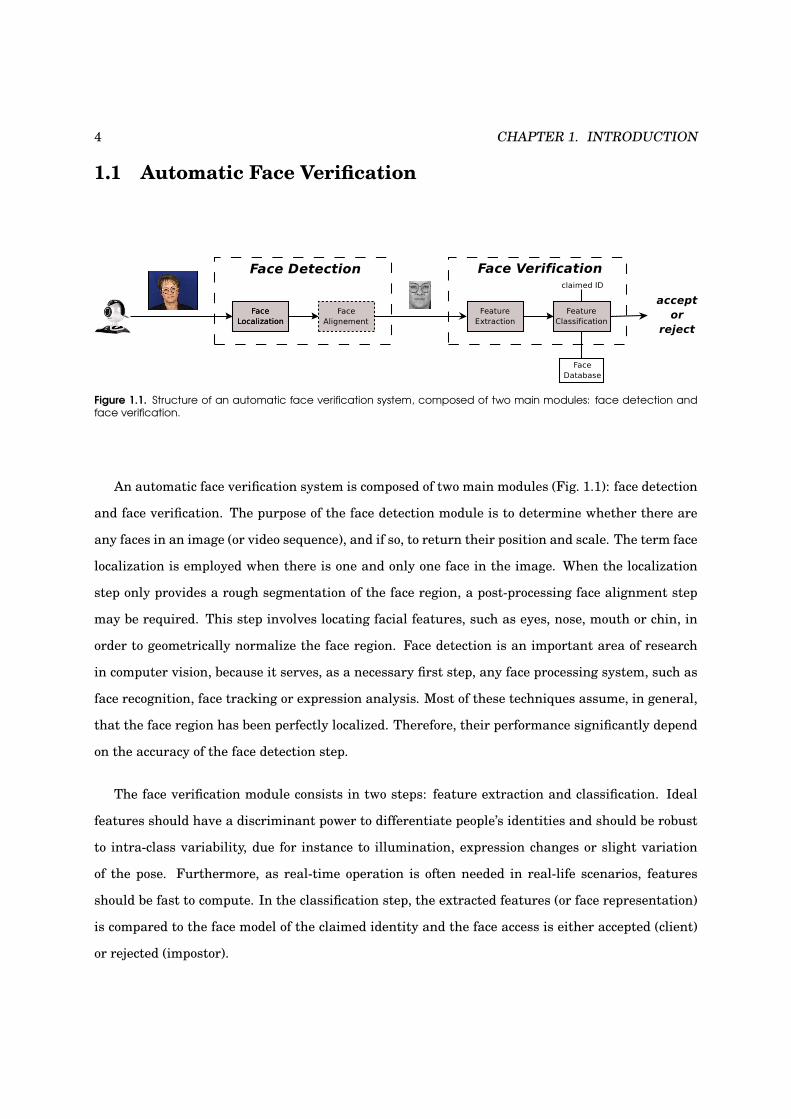
Figure 1.1. Structure of an automatic face verification system, composed of two main modules: face detection andface verification.
An automatic face verification system is composed of two main modules (Fig. 1.1): face detection
and face verification. The purpose of the face detection module is to determine whether there are
any faces in an image (or video sequence), and if so, to return their position and scale. The term face
localization is employed when there is one and only one face in the image. When the localization
step only provides a rough segmentation of the face region, a post-processing face alignment step
may be required. This step involves locating facial features, such as eyes, nose, mouth or chin, in
order to geometrically normalize the face region. Face detection is an important area of research
in computer vision, because it serves, as a necessary first step, any face processing system, such as
face recognition, face tracking or expression analysis. Most of these techniques assume, in general,
that the face region has been perfectly localized. Therefore, their performance significantly depend
on the accuracy of the face detection step.
The face verification module consists in two steps: feature extraction and classification. Ideal
features should have a discriminant power to differentiate people’s identities and should be robust
to intra-class variability, due for instance to illumination, expression changes or slight variation
of the pose. Furthermore, as real-time operation is often needed in real-life scenarios, features
should be fast to compute. In the classification step, the extracted features (or face representation)
is compared to the face model of the claimed identity and the face access is either accepted (client)
or rejected (impostor).

1.2. CHALLENGES 5
1.2 Challenges
Although face detection receives considerable attention, it still remains a difficult pattern recog-
nition task, because of the high variability of the face appearance. Faces are non-rigid, dynamic
objects with a large diversity in shape, color and texture, due to multiple factors such as head pose,
lighting conditions (contrast, shadows), facial expressions, occlusions (glasses) and other facial fea-
tures (make-up, beard).
Large variability in face appearance also affects face verification. Furthermore, quoting Moses et
al., "the variations between the images of the same face due to illumination and viewing direction
are almost always larger than the image variation due to change in face identity" [70]. Another
difficulty comes from the lack of reference images to train face templates. In real-life applications,
the enrolment procedure has to be fast and is generally done once. The few available training data
are usually not enough to cover the intra-personal variability of the face. Moreover a significant
mismatch between training and testing conditions may happen (especially lighting). Finally, the
verification performance is highly related to the quality of the face localization step.
1.3 Scope and Contributions
This thesis aims to build a fully automatic face verification system which works in real-time. The
system must be robust enough to small head pose and lighting variations in order to be used in a
real-life low level application such as computer access log-in. Most research has been done in face
detection, face alignment and face verification, but few works treat these distinct modules as an
ensemble. Most of the papers on face detection do not consider the final application for which the
detector is designed and most of the papers on face verification assume a perfect localization of the
face, which is not realistic. In this thesis, we consider the automatic face verification as a unified
task. The main contributions of this work are briefly presented in the following:
• performance evaluation of face detection systems [80]: several aspects make perfor-
mance comparisons very difficult. We underline the importance of a unified face criterion,
assessing what is a correctly detected face, when reporting detection rates. We also show how
the image scanning process, the overlapped detections merging or even the size of the training

6 CHAPTER 1. INTRODUCTION
dataset may affect the performance of a detection system.
• multiview face detection [93]: we propose a novel architecture, based on a pyramid of de-
tectors trained for each view. Individual detectors are based on the boosting of Local Binary
Pattern (LBP) features. The system works in real-time and shows high performance on bench-
mark test sets. Compared to traditional approaches based on Haar-features [105], the detector
is more robust to illumination changes and partial occlusion of the face.
• face verification [84]: we propose a new generative approach based on the adaptation of
LBP histograms. Generative approaches have proven to be more effective than discriminative
ones, mainly because of the lack of training data. Our system shows improved performance
compared to other state-of-the-art LBP based techniques.
• face alignment [59]: we extend the Active Shape Model (ASM) [13] method by using an LBP
representation instead of pixel intensities. The LBP-ASM system achieves more accurate
alignment and is more robust to illumination.
• system-dependent performance measure [82, 83]: we explain that face localization errors
may have different impacts depending on the final application. We analyze the effect of the
different kinds of localization errors (shift, scale, rotation) on the specific task of face verifi-
cation. To properly evaluate the performance of face localization algorithms, we propose to
embed the final application (here verification) into the performance measuring process. We
empirically demonstrate that the proposed measure gives a better estimate of the quality of
the face localization step.
• demonstrators [60]: based on the findings of this thesis, we built several demonstrators,
such as a bi-modal (face and speech) biometric demonstrator, a computer access log-in and a
face tracking system.
• Torch3vision: it is an open source machine vision library, written in simple C++, designed for
scientific research. It includes standard image processing and feature extraction algorithms
and is available from: http://torch3vision.idiap.ch/. All experiments in this thesis
have been implemented with Torch3vision.

1.4. ORGANIZATION OF THE THESIS 7
1.4 Organization of the Thesis
This thesis is organized as follows:
Chapter 2 addresses the problem of frontal face detection. The main previous approaches are
reviewed and a method based on boosting LBP features is presented. Special attention is also given
to the important issue of performance evaluation. (Papers V, VI)
Chapter 3 extends the frontal face detection system in order to deal with multiview faces. Some
recent approaches are reviewed and a novel pyramid architecture is introduced. Experimental
analysis is provided for different kinds of head rotations. (Paper X)
Chapter 4 describes a new face verification system based on the adaptation of LBP histograms.
Experimental evaluation is provided for both manual and automatic segmentation of the face. (Pa-
pers II, VII, IX)
Chapter 5 concerns the performance evaluation of face localization algorithms. It first analyzes
the effect of localization errors on the performance of a face verification system. It then presents
a new measure which takes into account the performance of the final application. An empirical
evaluation is provided for the particular case of face verification. (Papers I, V, VI)
Chapter 6 summarizes the main findings and remarks of the previous chapters and discusses
some ideas for future research.
Appendices present additional LBP-based works, respectively on face alignment (Appendix A,
Paper VIII), hand posture recognition (Appendix B, Paper IV) and image normalization (Appendix C,
Paper III), as well as some demonstrators on face detection and verification (Appendix D).

8 CHAPTER 1. INTRODUCTION
Chapter 2
Frontal Face Detection
Face detection is the first module of the automatic face verification system illustrated in Fig. 1.1. In
a verification scenario, we generally assume that the user will cooperate with the system, and thus
that the detection module will deal with frontal faces. This is the subject of this chapter.
We first present some previous approaches to the frontal face detection task (Section 2.1). Spe-
cial attention is given to boosting-based methods which have been so far the most effective in prac-
tice, both in terms of accuracy and speed. One of the main limitations in early boosting-based
approaches is the robustness to illumination and partial occlusion of the face. To cope with these
limitations, we propose to use Local Binary Pattern (LBP) features (Section 2.2). We also discuss
the fundamental problem of evaluating the quality of the face detection step, because its reliability
largely affects the performance of the whole verification system (Section 2.3). A detailed description
of the experimental setup is then provided (Section 2.4). While not mentioned in the majority of the
papers, experiments show that the scanning and overlapped detection merging processes may sig-
nificantly influence the accuracy and/or speed of the face detection process (Section 2.5). We finally
give some concluding remarks (Section 2.6).
2.1 Related Work
Numerous methods have been proposed to detect faces in images. Many of them are reviewed in
two recent survey papers by Yang et al. [111], and by Hjelmas and Low [33]. These methods can be
9

10 CHAPTER 2. FRONTAL FACE DETECTION
organized in two categories: feature-based approaches and appearance-based approaches.
Feature-based approaches make explicit use of face knowledge. They are usually based on the
detection of local features of the face, such as the nose, the mouth or the eyes, and the structural
relationship between these facial features. Feature-based methods are generally used for face lo-
calization (one face) in good quality images. They are robust to illumination conditions, occlusions
and viewpoint, but may also be computationnaly expensive.
Appearance-based approaches consider face detection as a two-class pattern recognition prob-
lem. They rely on statistical learning methods to build a face/nonface classifier from training sam-
ples. These methods are used for multiple face detections in lower image resolutions. Although
both classes of methods do not deal with the same problems and environments, appearance-based
approaches have recently received considerable attention and have proven to be more successful
and robust than feature-based approaches. We will discuss them in more detail hereafter.
2.1.1 Appearance-based Approaches
The concept of scanning window is the root idea of appearance-based methods. A sliding window
scans the input image at different locations and scales. Each subwindow is then given to a classifier
whose goal is to classify the subwindow as either face or nonface. The different appearance-based
methods mainly differ in the choice of this classifier. Among the most popular learning classifiers,
Support Vector Machines [75, 88, 79], Neural Networks [85, 112], Bayesian classifiers [14] or Hid-
den Markov Models [72] have been tried. Some of the most significant approaches are reported
below.
Turk and Pentland [101] proposed to perform Principal Component Analysis (PCA) on training
face images and to use the eigenvectors, also called eigenfaces, as a face template. A candidate sub-
window region is classified according to the distance computed in the PCA subspace after projection.
This distance can be interpreted as a measure of faceness.
Sung and Poggio [97] developed a distribution-based system which consists of two steps. First,
they partition the face distribution into 6 clusters, approximated by Gaussian functions, and de-
compose each cluster in the PCA subspace. The same is done to model the nonface distribution.
A distance is then computed between a candidate subwindow and its projection onto the PCA sub-
space for each of the 12 clusters. In a second step, a neural network is trained to classify face and

2.1. RELATED WORK 11
nonfaces based on these distances.
Rowley et al. [85] presented an ensemble of Neural Networks which works on pixel intensities
of candidate regions. Each network has a different structure with retinal connections to capture
the spatial relationships of pixels (facial features). Detections from individual networks are then
merged to provide the final classification decision.
Féraud et al. [19] proposed another Neural Network model, based on the Constrained Gen-
erative Model (CGM). CGMs are auto-associative connected Multi-Layer Perceptrons (MLP) with
three large layers of weights, trained to perform a non-linear PCA. Classification is obtained by
considering the reconstruction errors of the CGMs.
One of the most accurate face detector was reported by Roth et. al [112] who use the Sparse Net-
work of Winnows (SNoW) learning architecture. SNoW is a single layer Neural Network, composed
of linear threshold units, that uses the Littlestone’s Winnow update rule [50]. Their system uses
boolean features that encode the positions and intensity of pixels. A comparative analysis of SNoW
with Neural Networks and Support Vector Machines (SVM) can be found in [113] and [18].
Appearance-based methods reported above provide accurate detection results with few false
alarms. However, all of them need several seconds at best to process an image, mainly because
candidate subwindows need to be geometrically and photometrically normalized before classifica-
tion. This limitation is restrictive for real-life applications that need real-time face detection (> 15
frames per second).
In 2001, Viola and Jones [105] introduced the first real-time frontal face detection system. In-
stead of using pixel information, they proposed to use a new image representation and a set of
simple features that can be computed at any position and scale in constant time. Boosting learning
is both used for feature selection and classifier design. [105] is the first work of a new family of
face detection methods, called boosting-based methods, which we will describe in more details in
the next section.

12 CHAPTER 2. FRONTAL FACE DETECTION
2.1.2 Boosting-based Approaches
Boosting learning
Recently, most of the attention has been paid to boosting-based approaches since the famous work
of Viola and Jones [105]. These approaches show very good results both in terms of accuracy and
speed, and are then well suited for real-time applications. The Viola and Jones face detector is
presented in more details in this section because a lot of recent work has concentrated on improving
this detector and because it will serve as a baseline comparison system in our experiments.
A complete introduction to the theoretical basis of boosting and its applications can be found
in [65]. The underlying idea of boosting is to linearly combine simple classifiers hj(X) to build a
strong ensemble H(X):
H(X) =
n∑
j=1
wjhj(X). (2.1)
The selection of the weak classifiers hj(X) as well as the estimation of the weights wj are learned
by the boosting procedure. Each classifier hj(X) aims to minimize the classification training error
on a particular distribution of the training samples. At each iteration (i.e. for each weak classifier),
the boosting procedure updates the weight of each sample such that the misclassified ones get more
weight in the next iteration. Boosting hence focuses on the examples that are hard to classify.
Several variants of Boosting exist. They mainly differ in the iterative reweigting process of the
training samples. AdaBoost [20] is probably the most well known.
Haar-like feature classifiers
In 2001, Pavlovic and Garg [77] proposed to boost pixel-based classifiers for face detection. Instead
of directly using pixel information, Viola and Jones introduce a set of simple features (Fig. 2.1),
derived from Haar wavelets. A feature is computed by summing the pixels in the white region and
Figure 2.1. Five types of Haar-like features.

2.1. RELATED WORK 13
subtracting those in the dark region. Haar-like features can be computed efficiently with the inte-
gral image representation or summed area table, first introduced by Crow [16] for texture mapping.
At a given location (x; y) in an image, the value of the integral image ii(x; y) is the sum of the pixels
above and to the left of (x; y):
ii(x; y) =∑
x′≤x,y′≤y
i(x′; y′),
where i(x′; y′) is the pixel value of the original image at location (x′; y′). If s(x; y) is the cumulative
row sum, with s(x;−1) = 0 and s(−1; y) = 0, the integral image can be computed in one pass over
the original image using the following pair of recurrences:
s(x; y) = s(x; y − 1) + i(x; y), (2.2)
ii(x; y) = ii(x − 1; y) + s(x; y). (2.3)
An example is given in Fig. 2.2. To compute the illustrated feature, only 6 table accesses and 7
simple operations are needed. Haar-like features can then be computed very quickly at any scale
and position in constant time.
BA
D FE
C
S S1 2
integral image
Figure 2.2. Haar-like feature computation with the integral image. The feature value is: S1−S2, with S1 = E−B−D+A
and S2 = F − C − E + B
The feature set is obtained by varying the size and position of each type of Haar-like features. To
select the weak classifiers hj(X) of Eq. 2.1, the learning procedure works as follows. Each candidate
feature fi is computed on a training set of positive and negative samples (faces and nonfaces).

14 CHAPTER 2. FRONTAL FACE DETECTION
The weak classifier then determines the optimal threshold θi which minimizes the classification
error. The task of the learning procedure is to find the feature f such that the minimum number of
samples are misclassified. A weak classifier hj(X) thus consists of a Haar-like feature f , a threshold
θ and a parity p indicating the direction of the inequality:
hj(X) =
1 if pf(X) < pθ,
0 otherwise.(2.4)
Such classifier can be seen as a single-node decision tree, also called decision stump.
Cascade architecture
Considering a set of images, the detection rate of a face detector is defined as the number of correctly
detected faces over the total number of faces in the test set. A false alarm is accounted each time
the system badly classifies a background region as a face. A higher detection rate (with less false
alarms) can be achieved by increasing the number n of weak classifiers hj(X) of the ensemble H(X)
of Eq. 2.1 . On the other hand, increasing n will also increase the complexity of the ensemble and
then the computation time.
To deal with the trade-off performance vs. computation time, Viola and Jones propose a cascade
structure of ensembles. This framework is motivated by the nature of the problem which is a rare
event detection problem. In an image, only a very small number of subwindows contain a face
(generally < 0.1%).
2τ>Mτ>
1τ<2τ<
Mτ<
1τ>M
H (x)
reject subwindow (Non Face)
Face
all candidatesubwindows
H (x)1
H (x)2
Figure 2.3. Overview of the cascade architecture which works as a degenerated decision tree. At each stage, theclassifier either rejects the sample and the process stops, or accepts it and the sample is forwarded to the next stage.

2.1. RELATED WORK 15
The cascade, illustrated in Fig. 2.3, works as follows: Each ensemble Hi(X) is designed to detect
almost all faces (>99%) while rejecting as much background regions as possible. This is done by
adjusting the thresholds τi on a validation set. The first ensemble H1(X), composed of only two
features, rejects approximately 50% of the background subwindows. As the task becomes more
difficult, the next ensembles contain more weak classifiers. With such a simple-to-complex ap-
proach, most of the background regions are quickly discarded early in the cascade and only face
subwindows should pass over all the cascade. Viola and Jones compare a cascade of ten 20-feature
classifiers with a monolithic 200-feature classier. They report that the accuracy of both classifiers
is not significantly different, but that the cascade version performs almost 10 times faster.
2.1.3 Discussion
Since the work of Viola and Jones [105] published in 2001, most of the research in face detection
has focused on the improvement of their cascade architecture. Related works can be classified in
three directions, whether they provide alternative feature set, boosting algorithm or architecture
design.
Alternative boosting algorithms
At each iteration, AdaBoost selects the weak classifier which minimizes the (weighted) classification
error, regardless if the error is a false positive or false negative. The goal of the detection cascade
is however to achieve high detection rates (>99%) with moderate false alarm rates (>50%) for each
stage. In [106], Viola and Jones proposed a modified version of the original boosting algorithm,
called Asymmetric AdaBoost, which gives more weight to the positive examples. A very similar
cost-sensitive algorithm, CS-AdaBoost, has been published by Ma and Ding [56].
Wu et al. [108] also observed that AdaBoost is an indirect way to meet the learning goals of
the cascade. They proposed a cascade learning procedure based on direct forward feature selection
which is much faster than AdaBoost while yielding similar performance. McCane and Novins [64]
also proposed an alternative to boosting. They explained that since the feature set is parame-
terizable (size and position of the Haar-like masks), the feature selection is a form of numerical
optimization, and they provided a fast (300-fold) heuristic to find (suboptimal) features.
In [49], Lienhart et al. compared three boosting algorithms, Discrete, Real and Gentle AdaBoost,
16 CHAPTER 2. FRONTAL FACE DETECTION
and showed that the latter performs slightly better. However, according to [9], the choice of the
boosting algorithm has more impact on the speed of the detector than on classification performance.
Li et al. [46] proposed a new boosting algorithm, called FloatBoost, to solve the monotonicity
problem encountered in the sequential forward search procedure of AdaBoost. After each iteration,
FloatBoost removes the least significant weak classifier which leads to a higher error rate of the
global classifier. Compared to the sequential AdaBoost, FloatBoost needs fewer weak classifiers
to achieve the same error rate. The cost of such improvement is a learning time of about 5 times
longer.
Other variants of AdaBoost have been tried for face detection, like Kullback-Leibler Boost-
ing [51], LogitBoost [21], Jensen-Shannon Boosting [37], Vector Boosting [34] or MRC-Boosting [110]
Alternative feature sets
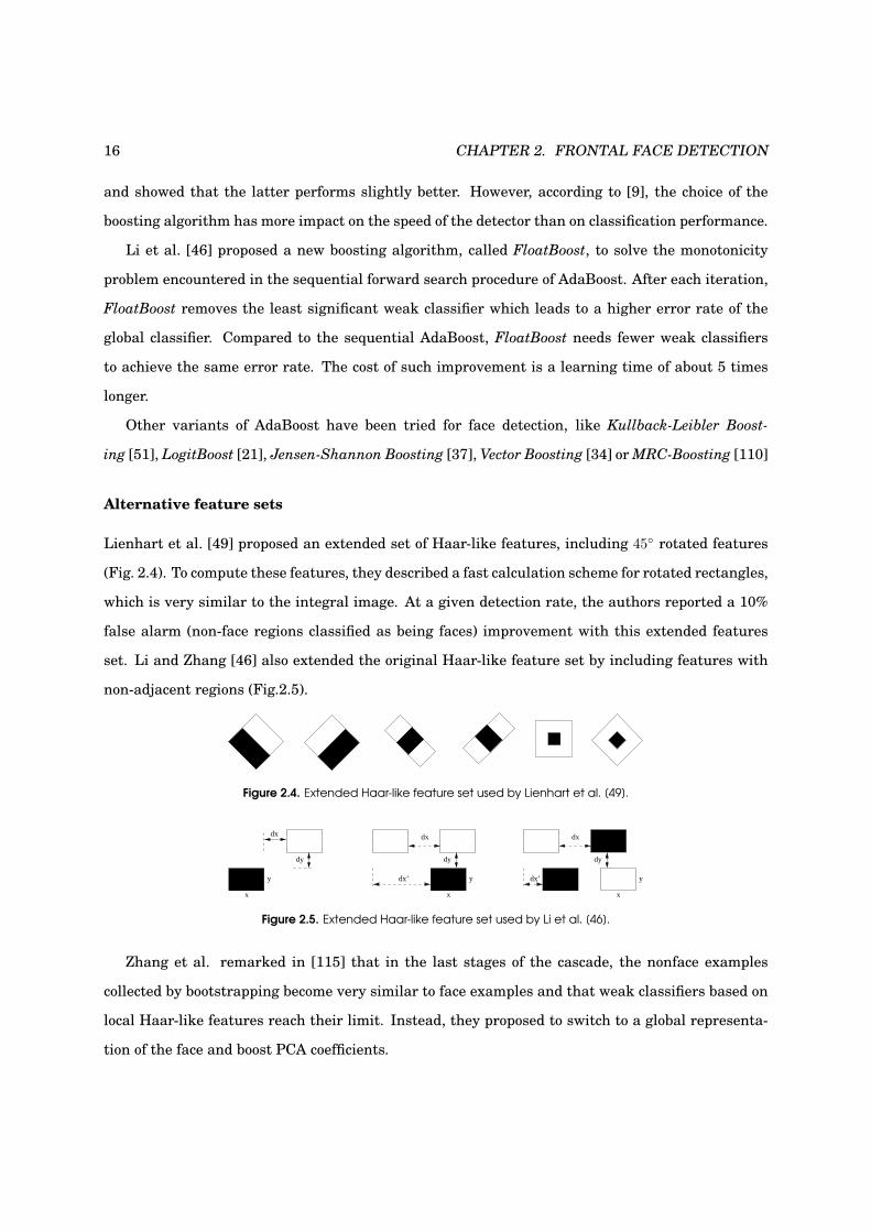
Lienhart et al. [49] proposed an extended set of Haar-like features, including 45 rotated features
(Fig. 2.4). To compute these features, they described a fast calculation scheme for rotated rectangles,
which is very similar to the integral image. At a given detection rate, the authors reported a 10%
false alarm (non-face regions classified as being faces) improvement with this extended features
set. Li and Zhang [46] also extended the original Haar-like feature set by including features with
non-adjacent regions (Fig.2.5).
Figure 2.4. Extended Haar-like feature set used by Lienhart et al. [49].
dx
dy
dx’
x
y
dx
dy
y
x
dx’
dx
dy
y
x
Figure 2.5. Extended Haar-like feature set used by Li et al. [46].
Zhang et al. remarked in [115] that in the last stages of the cascade, the nonface examples
collected by bootstrapping become very similar to face examples and that weak classifiers based on
local Haar-like features reach their limit. Instead, they proposed to switch to a global representa-
tion of the face and boost PCA coefficients.

2.1. RELATED WORK 17
Mita et al. [68] proposed new features based on co-occurrence of multiple Haar-like features,
called joint Haar-like features, which capture the structural similarities within the face class. Given
the same number of features, they reported improved performance compared to the original system.
In [22], Fröba and Ernst used a Modified version of the Census Transform (MCT) to build weak
classifiers, while Hadid et al. [29], Jin et al. [40] or Zhang et al. [117] chose LBP features (cf.
Section 2.2.1).
Alternative cascade architecture
The two main limitations of the detector of Viola and Jones [105] are a long training procedure and
the choice of the cascade parameters. A lot of effort has been given on finding training alternatives,
but much less attention has been paid to the fundamental problem of the cascade architecture
design.
In [54], Luo published a method to adjust the stage thresholds after the training of the cascade.
He reported improved performance compared to the original Viola and Jones detector. However,
his post-processing technique does not help to chose the threshold values during training and then
does not solve the problem of when to stop training the current stage and go for the next one.
McCane and Novins [64] pointed out that the root idea of the cascade architecture is to quickly
discard nonface subwindows. Since there are much less faces than nonfaces regions, the speed of
the detector can be seen as the average speed to reject a nonface subwindow. McCane and Novins
argued that the speed of the detector is the function to minimize and proposed a method to deter-
mine the optimal cascade speed.
Grossman [28] first trained a single-stage classifier with AdaBoost. Using dynamic program-
ming, he then partitioned the weak classifiers of this single stage to build a cascade of optimal
speed with almost identical behavior to the original single-stage classifier. The main drawback
of Grossman’s method is to produce more false alarms, because it does not take advantage of the
bootstrapping technique of the original cascade training approach.
Li and Satoh [45] proposed to sequentially combine a classical boosted cascade with a cascade
of three SVM classifiers, trained with the features selected by AdaBoost in the last stage of the
classical cascade.
Lienhart et al. [49] tried Classification And Regression decision Trees (CART) as weak clas-

18 CHAPTER 2. FRONTAL FACE DETECTION
sifiers instead of simple decision stumps (Eq. 2.1). They reported improved results for the same
computation time.
Wu et al. [107] described a nested cascade structure. The difference with the classical cascade
approach is that each layer is used as the first weak classifier of the following layer, thus retaining
the discriminative power of previous layers (confidence of the predecessor). A similar approach was
proposed by Xiao et al. [109].
Brubaker et al. [9] introduced a new criterion for cascade training to select stage thresholds
(balance between detection and false alarm rates) and number of weak classifiers (when to stop
training in one stage and move on to the next one), based on a probabilistic model of the overall cas-
cade’s performance. They also evaluated several feature selection methods to speed up the training
process and investigated CART as weak classifiers.
2.2 Frontal Face Detection Using Local Binary Patterns
The face detection algorithm introduced in this section is an extension of Viola and Jones sys-
tem [105] based on boosted cascades of Haar-like features. As pointed out by Zhang et al. [115],
these features are very efficient early in the cascade to quickly discard most of the background
regions. However, in the last stages of the cascade, a large number of Haar-like features (several
hundreds) are necessary to reach the desired detection/false acceptance rate trade-off. It results in
a long training procedure and cascades with several dozens of stages which are difficult to design.
Furthermore, Haar-like features are not robust to local illumination changes.
To cope with the limitation of Haar-like features, we propose to use LBP features (Section 2.2.1).
The method to build the weak classifiers is inspired by the work of Fröba and Ernst [22] and the
cascade training is done with AdaBoost [20] (Section 2.2.2).
2.2.1 LBP Features
The LBP operator is a non-parametric 3x3 kernel which summarizes the local spacial structure of
an image. It was first introduced by Ojala et al. [73] who showed the high discriminative power of
this operator for texture classification. At a given pixel position (xc, yc), LBP is defined as an ordered
set of binary comparisons of pixel intensities between the center pixel and its eight surrounding
2.2. FRONTAL FACE DETECTION USING LOCAL BINARY PATTERNS 19
83 75 126
99 95 141
91 91 100
0 0
0 10
1
1
1 binary: 00111001decimal: 57
comparisonwith the center
binary intensity
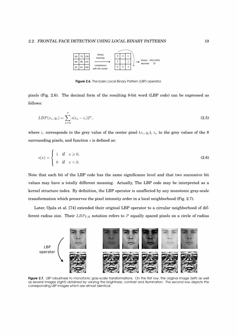
Figure 2.6. The basic Local Binary Pattern (LBP) operator.
pixels (Fig. 2.6). The decimal form of the resulting 8-bit word (LBP code) can be expressed as
follows:
LBP (xc, yc) =7
∑
n=0
s(in − ic)2n, (2.5)
where ic corresponds to the grey value of the center pixel (xc, yc), in to the grey values of the 8
surrounding pixels, and function s is defined as:
s(x) =
1 if x > 0,
0 if x < 0.(2.6)
Note that each bit of the LBP code has the same significance level and that two successive bit
values may have a totally different meaning. Actually, The LBP code may be interpreted as a
kernel structure index. By definition, the LBP operator is unaffected by any monotonic gray-scale
transformation which preserves the pixel intensity order in a local neighborhood (Fig. 2.7).
Later, Ojala et al. [74] extended their original LBP operator to a circular neighborhood of dif-
ferent radius size. Their LBPP,R notation refers to P equally spaced pixels on a circle of radius
Figure 2.7. LBP robustness to monotonic gray-scale transformations. On the first row, the original image (left) as wellas several images (right) obtained by varying the brightness, contrast and illumination. The second row depicts thecorresponding LBP images which are almost identical.
20 CHAPTER 2. FRONTAL FACE DETECTION
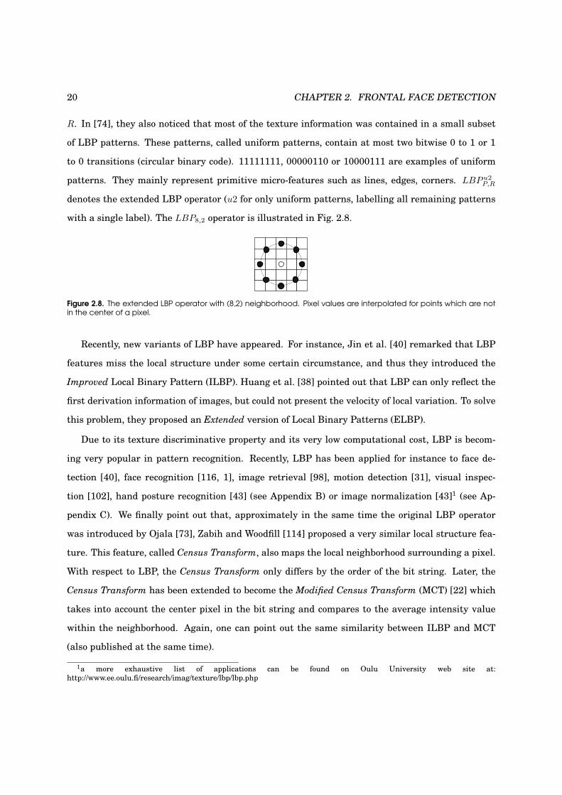
R. In [74], they also noticed that most of the texture information was contained in a small subset
of LBP patterns. These patterns, called uniform patterns, contain at most two bitwise 0 to 1 or 1
to 0 transitions (circular binary code). 11111111, 00000110 or 10000111 are examples of uniform
patterns. They mainly represent primitive micro-features such as lines, edges, corners. LBPu2P,R
denotes the extended LBP operator (u2 for only uniform patterns, labelling all remaining patterns
with a single label). The LBP8,2 operator is illustrated in Fig. 2.8.
Figure 2.8. The extended LBP operator with (8,2) neighborhood. Pixel values are interpolated for points which are notin the center of a pixel.
Recently, new variants of LBP have appeared. For instance, Jin et al. [40] remarked that LBP
features miss the local structure under some certain circumstance, and thus they introduced the
Improved Local Binary Pattern (ILBP). Huang et al. [38] pointed out that LBP can only reflect the
first derivation information of images, but could not present the velocity of local variation. To solve
this problem, they proposed an Extended version of Local Binary Patterns (ELBP).
Due to its texture discriminative property and its very low computational cost, LBP is becom-
ing very popular in pattern recognition. Recently, LBP has been applied for instance to face de-
tection [40], face recognition [116, 1], image retrieval [98], motion detection [31], visual inspec-
tion [102], hand posture recognition [43] (see Appendix B) or image normalization [43]1 (see Ap-
pendix C). We finally point out that, approximately in the same time the original LBP operator
was introduced by Ojala [73], Zabih and Woodfill [114] proposed a very similar local structure fea-
ture. This feature, called Census Transform, also maps the local neighborhood surrounding a pixel.
With respect to LBP, the Census Transform only differs by the order of the bit string. Later, the
Census Transform has been extended to become the Modified Census Transform (MCT) [22] which
takes into account the center pixel in the bit string and compares to the average intensity value
within the neighborhood. Again, one can point out the same similarity between ILBP and MCT
(also published at the same time).
1a more exhaustive list of applications can be found on Oulu University web site at:
http://www.ee.oulu.fi/research/imag/texture/lbp/lbp.php
2.2. FRONTAL FACE DETECTION USING LOCAL BINARY PATTERNS 21
In this chapter, we will consider the ILBP version (or MCT), described in [40] (or in [22]), which
outputs a 9-bit word (ILBP code). In the rest of this chapter, we will use the LBP notation to refer
to ILBP (or MCT) features.
2.2.2 Weak Classifiers and Cascade Training
Weak classifiers
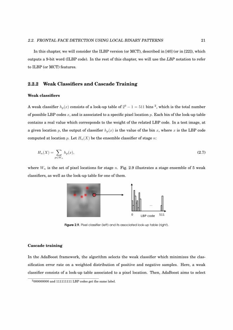
A weak classifier hp(x) consists of a look-up table of 29 − 1 = 511 bins 2, which is the total number
of possible LBP codes x, and is associated to a specific pixel location p. Each bin of the look-up table
contains a real value which corresponds to the weight of the related LBP code. In a test image, at
a given location p, the output of classifier hp(x) is the value of the bin x, where x is the LBP code
computed at location p. Let Hn(X) be the ensemble classifier of stage n:
Hn(X) =∑
p∈Wn
hp(x), (2.7)
where Wn is the set of pixel locations for stage n. Fig. 2.9 illustrates a stage ensemble of 5 weak
classifiers, as well as the look-up table for one of them.
Figure 2.9. Pixel classifier (left) and its associated look-up table (right).
Cascade training
In the AdaBoost framework, the algorithm selects the weak classifier which minimizes the clas-
sification error rate on a weighted distribution of positive and negative samples. Here, a weak
classifier consists of a look-up table associated to a pixel location. Then, AdaBoost aims to select
2000000000 and 111111111 LBP codes get the same label.

22 CHAPTER 2. FRONTAL FACE DETECTION
pixel locations and to build the associated look-up tables. The training algorithm is detailed in [22]
and is explained below.
At each stage n of the cascade, the number Pn of weak classifiers is fixed, as well as the number
Tn of boosting iterations. Pn is then the size of the set of pixel locations Wn.
At each boosting iteration t, to select the best pixel classifier, two look-up tables Lfacep and
Lnonfacep are allocated for each pixel location of Wn. Then, for each location p, the LBP operator
is applied on a training set of face samples. For each sample, the computed LBP code is used to
identify the bin of Lfacep , which is increased by an amount equal to the weight of the sample. The
same is done with a training set of nonfaces to populate the Lnonfacep tables. The classification error
ε at position p is given by:
εp =511∑
j=1
min(Lfacep [j], Lnonface
p [j]). (2.8)
The look-up table Lp∗ of the selected pixel classifier at iteration t is then computed for each bin j:
Lp∗ [j] =
1 if Lfacep [j] > Lnonface
p [j],
0 otherwise.(2.9)
A pixel classifier thus consists of a look-up table of 0s and 1s. During the boosting learning, a
discriminative pixel location may be selected several times. At the end of the boosting procedure,
look-up tables associated to the same pixel location are merged into a single table. For each bin, a
weighted (by coefficient wt of AdaBoost, Eq. 2.1) sum is done on the bin values of each table. Weak
classifiers hp(x) of Eq. 2.7 consist of these single weighted look-up tables.
Note that this boosted cascade of LBP framework has been successfully applied to the task of
hand posture recognition [43] and described in Appendix B.

2.3. PERFORMANCE EVALUATION 23
2.3 Performance Evaluation
2.3.1 Performance Measure
On a given test database, the performance of a face detection system is measured in terms of De-
tection Rate (DR), which is the proportion of faces detected, and the number of False Acceptances
(nFA), which is the number of background regions badly classified as face regions. DR and nFA
are related. Increasing (resp. decreasing) DR usually means increasing (resp. decreasing) nFA as
well. Then, instead of providing a single operating point, it is more appropriate to provide the Free
Receiver Operator Characteristic (FROC) curve, which plots DR versus nFA. The ROC curve is very
similar. It represents the detection rate versus the false acceptance rate. However, the ROC curve
is not adapted for face detection because the false acceptance rate, which is defined as the number
of false acceptances over the total number of scanned windows containing no face, depends on the
scanning process.
2.3.2 Face Criterion
Reporting detection and error rates is not enough to allow fair performance comparisons. The way
detections and errors are accounted should also be clearly described. In other words, a face criterion,
assessing what is a correctly detected face, should be defined. Fig. 2.10 illustrates the problem.
Some people will account five correct face detections, while other people, using a more restrictive
face criterion, will only report the detection on the left. Recently, Jesorsky et al. [39] introduced a
relative error measure based on the distance between the detected and the expected (ground-truth)
eye center positions. Let Cl (respectively Cr) be the true left (resp. right) eye coordinate position
and let Cl (resp. Cr) be the left (resp. right) eye position estimated by the face detection algorithm.
Figure 2.10. Examples of various detections of the same face. Which one is a correct detection?

24 CHAPTER 2. FRONTAL FACE DETECTION
This measure can be written as:
deye =max(d(Cl, Cl), d(Cr, Cr))
d(Cl, Cr)(2.10)
where d(a, b) is the Euclidean distance between positions a and b. A successful detection is ac-
counted if deye < 0.25, which corresponds approximately to half the width of an eye. This is, to
the best of our knowledge, the first attempt to provide a unified face localization measure. This
fundamental problem of face criterion is analyzed in Chapter 5.
2.3.3 Application-dependent Evaluation
The performance evaluation should depend on the purpose of the detector. The balance between
detection rate, number of false acceptances and speed should be properly weighted. If the detector
is used for face recognition, the detection rate must be maximized, to the detriment of the number
of false acceptance which will be rejected by the recognition process. On the other hand, if the
detector is used for active tracking in video conferencing, accuracy may need to be sacrificed for
speed. One may use temporal information to refine the accuracy and remove false acceptances. A
clear description of the scenario (final application) and of the evaluation protocol (DR, nFA, speed)
is needed when assessing the performance of face detection systems.
2.4 Experimental Setup
2.4.1 Training Data
Appearance-based face detection methods highly rely on the training sets to find a discriminant
function between face and nonface classes. Robustness to appearance variability of the face is
achieved by incorporating this variability into the training set. For instance, to detect the face of
people wearing glasses, several samples of faces with glasses are added into the face training set.
We proceed similarly to deal with small pose variations of the head, facial expressions, people gen-
der, aging and so on. Actually, the richness of the training set is fundamental for the performance
of the face detector system.

2.4. EXPERIMENTAL SETUP 25
Faces
Many face databases are available on the Internet. Among them, we selected face images from
BANCA [3] (Spanish corpus), Essex 3, Feret [78], ORL [89], Stirling4 and Yale [6] databases. The
extraction of each face is done as follows:
1. Each face is labelled by manually locating the center position of both eyes. These two land-
mark points (groundtruth) are used to geometrically align the faces.
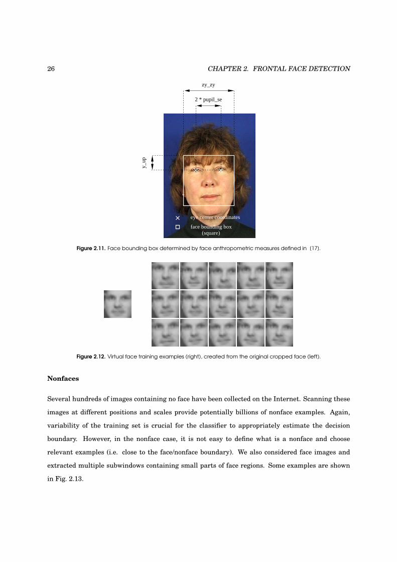
2. Face/head anthropometric measures are used to determine the face bounding box and crop the
face region. The width bbxw of this region (in pixels) is defined by:
bbxw =zy_zy
2 ∗ pupil_se∗ dGT (2.11)
where dGT is the distance (in pixels) between both eye centers, and zy_zy = 139.1 (mean width
of a human face in [mm]) and pupile_se = 33.4 (half of the inter-pupil distance in [mm]) are
anthropometric constants given by Farkas in [17]. According to Fig 2.11 and given y_up =
pupile_se, the position of the bounding box can be computed.
3. The cropped face is then subsampled to the size of 19x19 pixels. This template size was also
used by Sung et al. [97], Papageorgiou et al. [76] or Osuna et al. [75], while Rowley [85]
chose a template of 20x20 and Viola and Jones [105] a template of 24x24. In his thesis [15],
Cristinacce showed that the choice of an optimal face template size is not trivial. The set of
faces is then split in two sets of equal size (training and validation).
The concept of scanning window is a discrete process. Due to time constraints, a test image can
not be scanned at each position and scale. To detect faces which do not exactly fit the scanning
window, small localization errors are artificially generated by slightly shifting, scaling and rotating
the original face. Training and validation sets can be further extended by mirroring each face
example (Fig. 2.12). From each original face image, 10 virtual samples are randomly created.
3images available from: http://cswww.essex.ac.uk/mv/allfaces/index.html4images available from: http://pics.psych.stir.ac.uk/
26 CHAPTER 2. FRONTAL FACE DETECTION
face bounding box
eye center coordinates
2 * pupil_se
zy_zy
y_up
(square)
Figure 2.11. Face bounding box determined by face anthropometric measures defined in [17].
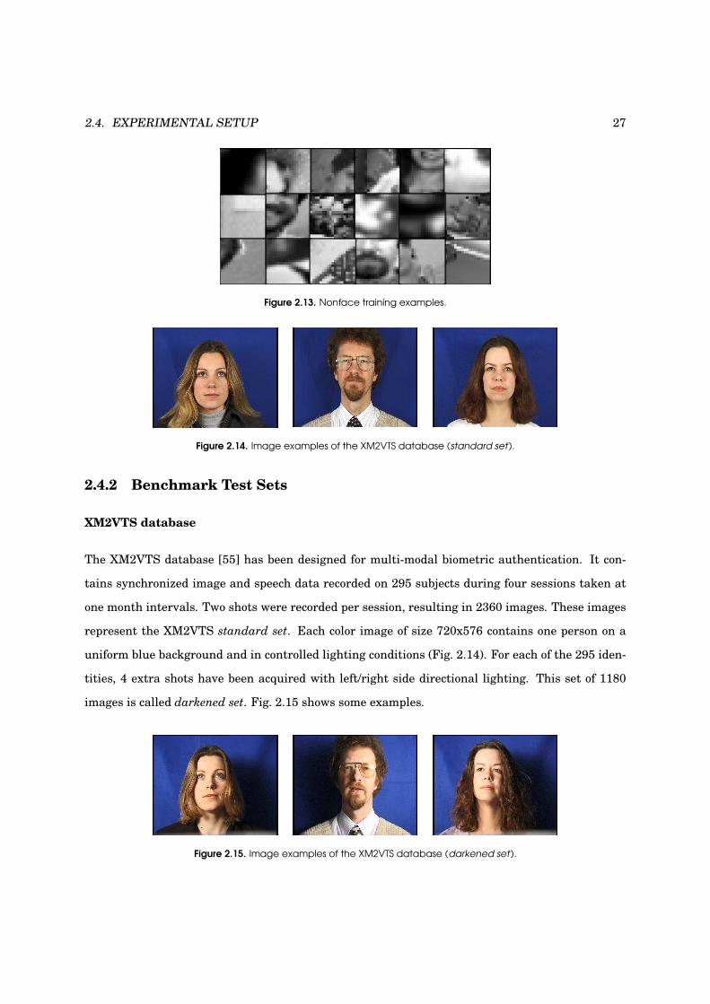
Figure 2.12. Virtual face training examples (right), created from the original cropped face (left).
Nonfaces
Several hundreds of images containing no face have been collected on the Internet. Scanning these
images at different positions and scales provide potentially billions of nonface examples. Again,
variability of the training set is crucial for the classifier to appropriately estimate the decision
boundary. However, in the nonface case, it is not easy to define what is a nonface and choose
relevant examples (i.e. close to the face/nonface boundary). We also considered face images and
extracted multiple subwindows containing small parts of face regions. Some examples are shown
in Fig. 2.13.
2.4. EXPERIMENTAL SETUP 27
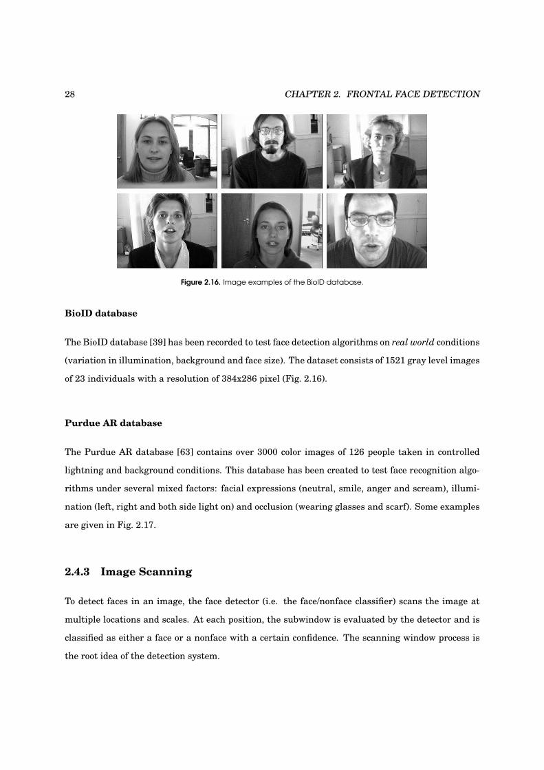
Figure 2.13. Nonface training examples.
Figure 2.14. Image examples of the XM2VTS database (standard set).
2.4.2 Benchmark Test Sets
XM2VTS database
The XM2VTS database [55] has been designed for multi-modal biometric authentication. It con-
tains synchronized image and speech data recorded on 295 subjects during four sessions taken at
one month intervals. Two shots were recorded per session, resulting in 2360 images. These images
represent the XM2VTS standard set. Each color image of size 720x576 contains one person on a
uniform blue background and in controlled lighting conditions (Fig. 2.14). For each of the 295 iden-
tities, 4 extra shots have been acquired with left/right side directional lighting. This set of 1180
images is called darkened set. Fig. 2.15 shows some examples.
Figure 2.15. Image examples of the XM2VTS database (darkened set).
28 CHAPTER 2. FRONTAL FACE DETECTION
Figure 2.16. Image examples of the BioID database.
BioID database
The BioID database [39] has been recorded to test face detection algorithms on real world conditions
(variation in illumination, background and face size). The dataset consists of 1521 gray level images
of 23 individuals with a resolution of 384x286 pixel (Fig. 2.16).
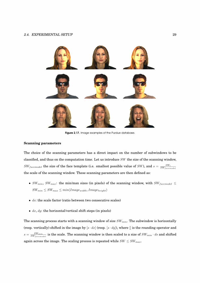
Purdue AR database
The Purdue AR database [63] contains over 3000 color images of 126 people taken in controlled
lightning and background conditions. This database has been created to test face recognition algo-
rithms under several mixed factors: facial expressions (neutral, smile, anger and scream), illumi-
nation (left, right and both side light on) and occlusion (wearing glasses and scarf). Some examples
are given in Fig. 2.17.
2.4.3 Image Scanning
To detect faces in an image, the face detector (i.e. the face/nonface classifier) scans the image at
multiple locations and scales. At each position, the subwindow is evaluated by the detector and is
classified as either a face or a nonface with a certain confidence. The scanning window process is
the root idea of the detection system.
2.4. EXPERIMENTAL SETUP 29
Figure 2.17. Image examples of the Purdue database.
Scanning parameters
The choice of the scanning parameters has a direct impact on the number of subwindows to be
classified, and thus on the computation time. Let us introduce SW the size of the scanning window,
SWfacemodel the size of the face template (i.e. smallest possible value of SW ), and s = SWi
SWfacemodel
the scale of the scanning window. These scanning parameters are then defined as:
• SWmin, SWmax: the min/max sizes (in pixels) of the scanning window, with SWfacemodel ≤
SWmin ≤ SWmax ≤ min(Imagewidth, Imageheight)
• ds: the scale factor (ratio between two consecutive scales)
• dx, dy: the horizontal/vertical shift steps (in pixels)
The scanning process starts with a scanning window of size SWmin. The subwindow is horizontally
(resp. vertically) shifted in the image by [s · dx] (resp. [s · dy]), where [] is the rounding operator and
s = SWmin
SWfacemodelis the scale. The scanning window is then scaled to a size of SWmin · ds and shifted
again across the image. The scaling process is repeated while SW ≤ SWmax.

30 CHAPTER 2. FRONTAL FACE DETECTION
Two types of scanning
Scaling can be achieved in two different ways:
1. the image is iteratively subsampled, while the size of the scanning window is kept constant.
This method is referred to as pyramid scanning.
2. the scanning window is resized for each scale level, rather than subsampling the image. We
refer to this method as multiscale scanning.
When the computation cost to classify a subwindow does not depend on the size of the subwindow
(scale invariant), the multiscale mode is much faster, because no image subsampling nor subwin-
dow cropping is needed. Features based on summed area of pixels, like Haar-like or LBP features,
can be computed in constant time at different scales with the integral image representation. Those
features are then candidates for multiscale scanning. On the other hand, features based on inde-
pendent pixel values can not take advantage of this scanning method (the pixel interpolation cost
is scale dependent). In this work, we will only use multiscale scanning.
2.4.4 Merging Overlapped Detections
Multiple detections at different locations and scales may occur around a face in the image, because
the face classifier is trained to be insensitive to small localization errors. The same behavior may
happen around a background region. However, overlapped false alarms usually appear with less
consistency than true detections. This assumption is useful to reduce the number of false alarms
and to combine true detections, as illustrated in Fig. 2.18. The image on the left shows a scanned
image with multiple detections around the face and some false alarms in the background. In the
image on the right, false alarms have been removed and the detections around the face have been
merged. After the image scanning, the processing of the multiple detections consists in two steps:
1. clustering: two detections belong to the same cluster if the detected regions overlap by a
given percentage φ. A cluster is a candidate for merging (next step) if the number of detec-
tions (or sum of confidence detection) is above a given threshold η. Another variant could
consider the aggregate confidence score (output of the classifier) of the detections instead of
their occurrence. If a cluster is not candidate, all detections of this cluster are removed.
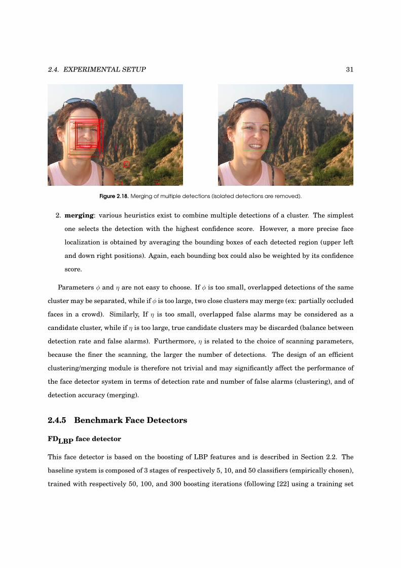
2.4. EXPERIMENTAL SETUP 31
Figure 2.18. Merging of multiple detections (isolated detections are removed).
2. merging: various heuristics exist to combine multiple detections of a cluster. The simplest
one selects the detection with the highest confidence score. However, a more precise face
localization is obtained by averaging the bounding boxes of each detected region (upper left
and down right positions). Again, each bounding box could also be weighted by its confidence
score.
Parameters φ and η are not easy to choose. If φ is too small, overlapped detections of the same
cluster may be separated, while if φ is too large, two close clusters may merge (ex: partially occluded
faces in a crowd). Similarly, If η is too small, overlapped false alarms may be considered as a
candidate cluster, while if η is too large, true candidate clusters may be discarded (balance between
detection rate and false alarms). Furthermore, η is related to the choice of scanning parameters,
because the finer the scanning, the larger the number of detections. The design of an efficient
clustering/merging module is therefore not trivial and may significantly affect the performance of
the face detector system in terms of detection rate and number of false alarms (clustering), and of
detection accuracy (merging).
2.4.5 Benchmark Face Detectors
FDLBP face detector
This face detector is based on the boosting of LBP features and is described in Section 2.2. The
baseline system is composed of 3 stages of respectively 5, 10, and 50 classifiers (empirically chosen),
trained with respectively 50, 100, and 300 boosting iterations (following [22] using a training set

32 CHAPTER 2. FRONTAL FACE DETECTION
and a validation set of ∼50.000 faces. The decision threshold of each stage has been chosen on
the face validation set to achieve 99% detection rate. On a 3GHz Pentium 4 with 1Go RAM, the
training of the whole cascade lasts around 5 hours. The scanning and overlap merging parameters
were chosen as follows:
• step x factor: dx = 0.05 (corresponds to a shift of 1 pixel for a bounding box of size 19 × 19)
• step y factor: dy = 0.10 (empirically chosen twice the step x factor)
• scale factor: ds = 1.125 (according to [105])
• min scanning window size: depends on the experiment
• min scanning window size: SWmax = size of the image
• surface overlap factor: φ = 0.5 (empirically chosen; depends on the step factors)
• detection confidence threshold: η = 1.5
FDHaar face detector
We use the face detector included in the OpenCV library available at: http://sourceforge.
net/projects/opencvlibrary/. The detector has been implemented by Lienhart and is related
to his paper [49]. We chose the model called alt tree. The 47-stage cascade is composed of 8468
Haar-like stump classifiers. We have no information on the training of the model (training set size,
threshold selection, face model, training duration, ..). Because the system only outputs bounding
boxes, we empirically estimated the coordinates of the eyes from the boxes by running the detector
on a set of simple face images and computing the average detected face image.
2.5 Frontal Face Detection Results
In this Section, face detection experiments will be done in localization mode (only one face per
image). For each detector, we only consider the detection with the highest confidence score. In order
to assess the localization accuracy of a system, cumulative distributions of Jesorsky’s deye metric are
reported (detection rate vs. deye). In a first set of experiments, we will compare FDLBP and FDHaar

2.5. FRONTAL FACE DETECTION RESULTS 33
detectors in several conditions: controlled (XM2VTS standard set), uncontrolled lighting (XM2VTS
darkened set), realistic office scenario (BioID), facial occlusions and expression variation (Purdue),
uncontrolled environment (BANCA English). In a second set of experiments, we will only consider
FDLBP and show the effect of several parameters such as scanning or merging parameters, which
may affect detection performance, both in terms of accuracy and speed.
In the following experiments, we will consider that system A is significantly better than system
B, when system A will give statistically better results than system B with a confidence level of
99%, with a standard proportion test, assuming a binomial distribution for the errors, and using a
normal approximation.
2.5.1 LBP vs. Haar Face Localization Results
Evaluation on the XM2VTS database (standard set)
The deye cumulative distributions were collected for FDLBP and FDHaar face detectors. The XM2VTS
database has been recorded in well controlled conditions (uniform background and frontal lighting).
Both systems are supposed to give similar performance. Fig. 2.19(a) confirms this assumption. For
deye ≤ 0.255, FDLBP achieves 99.5% detection rate compared to 97.7% for FDHaar.
Evaluation on the XM2VTS database (darkened set)
The XM2VTS darkened set set has been recorded with the same setup than the standard set, but
with directional lighting respectively illuminating the left and the right side of the face. We ex-
pect that the resulting shadows on the face should more affect the FDHaar system, because of the
sensitivity to local variations of pixel values. However, Fig. 2.19(b) shows that both systems are
similarly affected (97.5% compared to 99.5% for FDLBP and 95.7% compared to 97.7% for FDLBP ).
Both deye curves are very close for deye ≤ 0.10 and FDLBP looks better for deye > 0.10, although not
significantly.
5Jesorsky et al. [39] consider a face found if deye ≤ 0.25
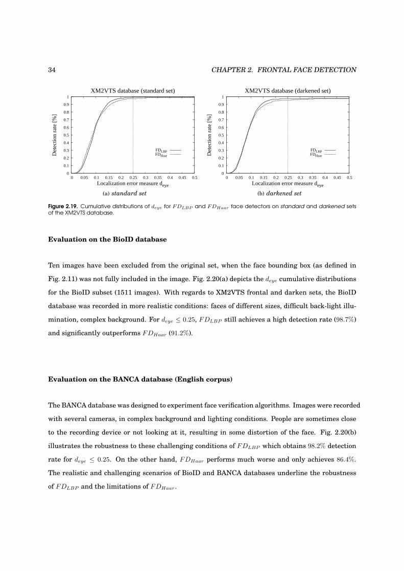
34 CHAPTER 2. FRONTAL FACE DETECTION
1
0.9
0.8
0.7
0.6
0.5
0.4
0.3
0.2
0.1
0 0.5 0.45 0.4 0.35 0.3 0.25 0.2 0.15 0.1 0.05 0
Det
ectio
n ra
te [
%]
Localization error measure deye
XM2VTS database (standard set)
FDLBPFDHaar
(a) standard set
1
0.9
0.8
0.7
0.6
0.5
0.4
0.3
0.2
0.1
0 0.5 0.45 0.4 0.35 0.3 0.25 0.2 0.15 0.1 0.05 0
Det
ectio
n ra
te [
%]
Localization error measure deye
XM2VTS database (darkened set)
FDLBPFDHaar
(b) darkened set
Figure 2.19. Cumulative distributions of deye for FDLBP and FDHaar face detectors on standard and darkened setsof the XM2VTS database.
Evaluation on the BioID database
Ten images have been excluded from the original set, when the face bounding box (as defined in
Fig. 2.11) was not fully included in the image. Fig. 2.20(a) depicts the deye cumulative distributions
for the BioID subset (1511 images). With regards to XM2VTS frontal and darken sets, the BioID
database was recorded in more realistic conditions: faces of different sizes, difficult back-light illu-
mination, complex background. For deye ≤ 0.25, FDLBP still achieves a high detection rate (98.7%)
and significantly outperforms FDHaar (91.2%).
Evaluation on the BANCA database (English corpus)
The BANCA database was designed to experiment face verification algorithms. Images were recorded
with several cameras, in complex background and lighting conditions. People are sometimes close
to the recording device or not looking at it, resulting in some distortion of the face. Fig. 2.20(b)
illustrates the robustness to these challenging conditions of FDLBP which obtains 98.2% detection
rate for deye ≤ 0.25. On the other hand, FDHaar performs much worse and only achieves 86.4%.
The realistic and challenging scenarios of BioID and BANCA databases underline the robustness
of FDLBP and the limitations of FDHaar.
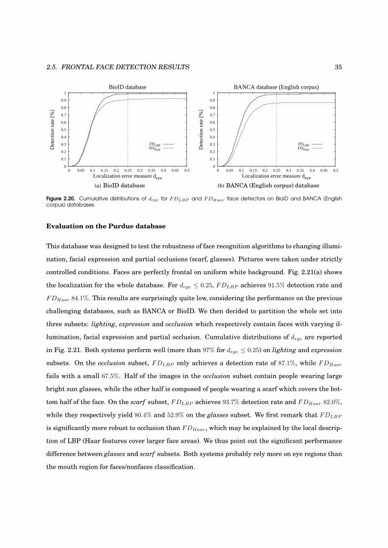
2.5. FRONTAL FACE DETECTION RESULTS 35
1
0.9
0.8
0.7
0.6
0.5
0.4
0.3
0.2
0.1
0 0.5 0.45 0.4 0.35 0.3 0.25 0.2 0.15 0.1 0.05 0
Det
ectio
n ra
te [
%]
Localization error measure deye
BioID database
FDLBPFDHaar
(a) BioID database
1
0.9
0.8
0.7
0.6
0.5
0.4
0.3
0.2
0.1
0 0.5 0.45 0.4 0.35 0.3 0.25 0.2 0.15 0.1 0.05 0
Det
ectio
n ra
te [
%]
Localization error measure deye
BANCA database (English corpus)
FDLBPFDHaar
(b) BANCA (English corpus) database
Figure 2.20. Cumulative distributions of deye for FDLBP and FDHaar face detectors on BioID and BANCA (Englishcorpus) databases.
Evaluation on the Purdue database
This database was designed to test the robustness of face recognition algorithms to changing illumi-
nation, facial expression and partial occlusions (scarf, glasses). Pictures were taken under strictly
controlled conditions. Faces are perfectly frontal on uniform white background. Fig. 2.21(a) shows
the localization for the whole database. For deye ≤ 0.25, FDLBP achieves 91.5% detection rate and
FDHaar 84.1%. This results are surprisingly quite low, considering the performance on the previous
challenging databases, such as BANCA or BioID. We then decided to partition the whole set into
three subsets: lighting, expression and occlusion which respectively contain faces with varying il-
lumination, facial expression and partial occlusion. Cumulative distributions of deye are reported
in Fig. 2.21. Both systems perform well (more than 97% for deye ≤ 0.25) on lighting and expression
subsets. On the occlusion subset, FDLBP only achieves a detection rate of 87.1%, while FDHaar
fails with a small 67.5%. Half of the images in the occlusion subset contain people wearing large
bright sun glasses, while the other half is composed of people wearing a scarf which covers the bot-
tom half of the face. On the scarf subset, FDLBP achieves 93.7% detection rate and FDHaar 82.0%,
while they respectively yield 80.4% and 52.9% on the glasses subset. We first remark that FDLBP
is significantly more robust to occlusion than FDHaar, which may be explained by the local descrip-
tion of LBP (Haar features cover larger face areas). We thus point out the significant performance
difference between glasses and scarf subsets. Both systems probably rely more on eye regions than
the mouth region for faces/nonfaces classification.
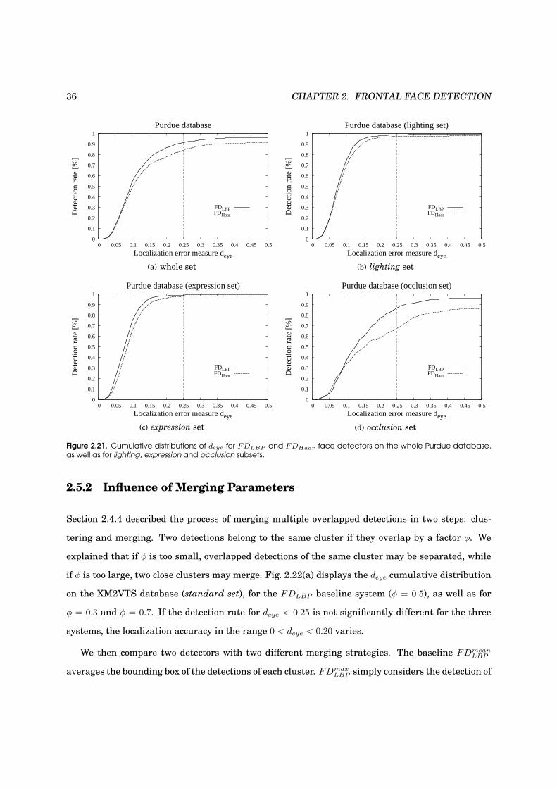
36 CHAPTER 2. FRONTAL FACE DETECTION
1
0.9
0.8
0.7
0.6
0.5
0.4
0.3
0.2
0.1
0 0.5 0.45 0.4 0.35 0.3 0.25 0.2 0.15 0.1 0.05 0
Det
ectio
n ra
te [
%]
Localization error measure deye
Purdue database
FDLBPFDHaar
(a) whole set
1
0.9
0.8
0.7
0.6
0.5
0.4
0.3
0.2
0.1
0 0.5 0.45 0.4 0.35 0.3 0.25 0.2 0.15 0.1 0.05 0
Det
ectio
n ra
te [
%]
Localization error measure deye
Purdue database (lighting set)
FDLBPFDHaar
(b) lighting set
1
0.9
0.8
0.7
0.6
0.5
0.4
0.3
0.2
0.1
0 0.5 0.45 0.4 0.35 0.3 0.25 0.2 0.15 0.1 0.05 0
Det
ectio
n ra
te [
%]
Localization error measure deye
Purdue database (expression set)
FDLBPFDHaar
(c) expression set
1
0.9
0.8
0.7
0.6
0.5
0.4
0.3
0.2
0.1
0 0.5 0.45 0.4 0.35 0.3 0.25 0.2 0.15 0.1 0.05 0
Det
ectio
n ra
te [
%]
Localization error measure deye
Purdue database (occlusion set)
FDLBPFDHaar
(d) occlusion set
Figure 2.21. Cumulative distributions of deye for FDLBP and FDHaar face detectors on the whole Purdue database,as well as for lighting, expression and occlusion subsets.
2.5.2 Influence of Merging Parameters
Section 2.4.4 described the process of merging multiple overlapped detections in two steps: clus-
tering and merging. Two detections belong to the same cluster if they overlap by a factor φ. We
explained that if φ is too small, overlapped detections of the same cluster may be separated, while
if φ is too large, two close clusters may merge. Fig. 2.22(a) displays the deye cumulative distribution
on the XM2VTS database (standard set), for the FDLBP baseline system (φ = 0.5), as well as for
φ = 0.3 and φ = 0.7. If the detection rate for deye < 0.25 is not significantly different for the three
systems, the localization accuracy in the range 0 < deye < 0.20 varies.
We then compare two detectors with two different merging strategies. The baseline FDmeanLBP
averages the bounding box of the detections of each cluster. FDmaxLBP simply considers the detection of
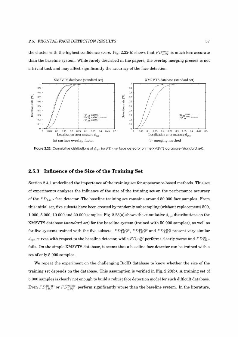
2.5. FRONTAL FACE DETECTION RESULTS 37
the cluster with the highest confidence score. Fig. 2.22(b) shows that FDmaxLBP is much less accurate
than the baseline system. While rarely described in the papers, the overlap merging process is not
a trivial task and may affect significantly the accuracy of the face detection.
1
0.9
0.8
0.7
0.6
0.5
0.4
0.3
0.2
0.1
0 0.5 0.45 0.4 0.35 0.3 0.25 0.2 0.15 0.1 0.05 0
Det
ectio
n ra
te [
%]
Localization error measure deye
XM2VTS database (standard set)
FDLBP surf 0.5FDLBP surf 0.3FDLBP surf 0.7
(a) surface overlap factor
1
0.9
0.8
0.7
0.6
0.5
0.4
0.3
0.2
0.1
0 0.5 0.45 0.4 0.35 0.3 0.25 0.2 0.15 0.1 0.05 0
Det
ectio
n ra
te [
%]
Localization error measure deye
XM2VTS database (standard set)
FDLBPmean
FDLBPmax
(b) merging method
Figure 2.22. Cumulative distributions of deye for FDLBP face detector on the XM2VTS database (standard set).
2.5.3 Influence of the Size of the Training Set
Section 2.4.1 underlined the importance of the training set for appearance-based methods. This set
of experiments analyzes the influence of the size of the training set on the performance accuracy
of the FDLBP face detector. The baseline training set contains around 50.000 face samples. From
this initial set, five subsets have been created by randomly subsampling (without replacement) 500,
1.000, 5.000, 10.000 and 20.000 samples. Fig. 2.23(a) shows the cumulative deye distributions on the
XM2VTS database (standard set) for the baseline system (trained with 50.000 samples), as well as
for five systems trained with the five subsets. FD20.000LBP , FD10.000
LBP and FD5.000LBP present very similar
deye curves with respect to the baseline detector, while FD1.000LBP performs clearly worse and FD500
LBP
fails. On the simple XM2VTS database, it seems that a baseline face detector can be trained with a
set of only 5.000 samples.
We repeat the experiment on the challenging BioID database to know whether the size of the
training set depends on the database. This assumption is verified in Fig. 2.23(b). A training set of
5.000 samples is clearly not enough to build a robust face detection model for such difficult database.
Even FD10.000LBP or FD20.000
LBP perform significantly worse than the baseline system. In the literature,
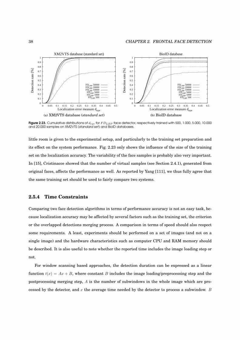
38 CHAPTER 2. FRONTAL FACE DETECTION
1
0.9
0.8
0.7
0.6
0.5
0.4
0.3
0.2
0.1
0 0.5 0.45 0.4 0.35 0.3 0.25 0.2 0.15 0.1 0.05 0
Det
ectio
n ra
te [
%]
Localization error measure deye
XM2VTS database (standard set)
FDLBP 50000FDLBP 20000FDLBP 10000
FDLBP 5000FDLBP 1000
FDLBP 500
(a) XM2VTS database (standard set)
1
0.9
0.8
0.7
0.6
0.5
0.4
0.3
0.2
0.1
0 0.5 0.45 0.4 0.35 0.3 0.25 0.2 0.15 0.1 0.05 0
Det
ectio
n ra
te [
%]
Localization error measure deye
BioID database
FDLBP 50000FDLBP 20000FDLBP 10000FDLBP 5000FDLBP 1000
FDLBP 500
(b) BioID database
Figure 2.23. Cumulative distributions of deye for FDLBP face detector, respectively trained with 500, 1.000, 5.000, 10.000and 20.000 samples on XM2VTS (standard set) and BioID databases.
little room is given to the experimental setup, and particularly to the training set preparation and
its effect on the system performance. Fig. 2.23 only shows the influence of the size of the training
set on the localization accuracy. The variability of the face samples is probably also very important.
In [15], Cristinacce showed that the number of virtual samples (see Section 2.4.1), generated from
original faces, affects the performance as well. As reported by Yang [111], we thus fully agree that
the same training set should be used to fairly compare two systems.
2.5.4 Time Constraints
Comparing two face detection algorithms in terms of performance accuracy is not an easy task, be-
cause localization accuracy may be affected by several factors such as the training set, the criterion
or the overlapped detections merging process. A comparison in terms of speed should also respect
some requirements. A least, experiments should be performed on a set of images (and not on a
single image) and the hardware characteristics such as computer CPU and RAM memory should
be described. It is also useful to note whether the reported time includes the image loading step or
not.
For window scanning based approaches, the detection duration can be expressed as a linear
function t(x) = Ax + B, where constant B includes the image loading/preprocessing step and the
postprocessing merging step, A is the number of subwindows in the whole image which are pro-
cessed by the detector, and x the average time needed by the detector to process a subwindow. B

2.6. CONCLUSION 39
can generally not be compressed and x concerns the optimization of the face/nonface classifier (ar-
chitecture design for cascade-based approaches). We describe below some techniques to reduce the
number of subwindows A:
• scanning parameters: Increasing the scanning parameters (see Section 2.4.3) will decrease A,
but usually at the cost of a loss in localization accuracy. A trade-off has to be found in practice.
• pruning: fast preprocessing methods can quickly discard subwindows before processing by the
classifier. For instance, thresholding the mean and standard deviation of pixels may easily
rejects uniform or too bright/dark regions. Skin color or edge filtering cues may also help.
• scanning tricks: instead of a constant horizontal or vertical shift step between two consecutive
subwindows, the amount of the shift can depends on the confidence score of the previous
subwindow.
• scanning techniques: in localization mode (one face), starting at a given (central) location and
at a given scale may largely speed-up the detection of the face.
In practical applications, other factors have to be taken into account, such as hardware (acquisition
device, image processing controller), source code/compilation optimizations, parallelization of the
image search. However, these factors are usually out of the research scope.
2.6 Conclusion
In this chapter, we gave an overview of recent methods in automatic face detection. Special at-
tention has been paid to boosting-based methods, which have been the most effective so far. The
main limitations of these approaches consist in long training procedures and the design of optimal
cascade architectures. We also showed the advantages of LBP features compared to the traditional
Haar-like features:
• the higher discriminative power of LBP allows similar error rates with much fewer features.
An effective system only needs about 200 LBP features distributed on 3 or 4 stages instead
of several thousands of Haar-like features on more than 30 stages. The training procedure is
then much shorter and the cascade design easier.

40 CHAPTER 2. FRONTAL FACE DETECTION
• LBP features are more robust to local illumination changes as well as to partial occlusion.
Experiments on BioID and BANCA databases underlined the limitation of Haar-like features
in difficult lighting conditions.
• LBP features can be computed quickly and take advantage of the integral image technique.
The fundamental issue of performance evaluation has also been discussed. We pointed out the
necessity of a standard face criterion to determine what is a correctly detected face when report-
ing error rates. However, even with a unified criterion, comparing face detection algorithms is
still tricky, because the performance of a system is affected by a wide range of factors such as the
training set, the image scanning parameters or the process of merging the overlapped detections.
Furthermore, in real-life applications, not only the accuracy but also the speed of the face detection
may be crucial.
Frontal face detection is now mature enough to be used in many practical applications. However,
performances are not comparable with those obtained by humans. It is still challenging to detect
partially occluded faces in a crowd in bad lighting conditions. In order to handle such limitations,
further improvements should consider additional feature sets with complementary discriminative
properties. However, the main challenge in face detection is to deal with head pose variations. This
is the subject of the next chapter.

Chapter 3
Multiview Face Detection
In real-life applications, faces are most of the time not in frontal view. Even with a cooperative
subject (verification scenario) the face is usually not perfectly frontal. An effective detector should
then be able to detect faces of varying head poses, called multiview faces. This chapter addresses
the problem of multiview face detection and extends the frontal system presented in Chapter 2.
We will first review recent state-of-the art approaches to the multiview face detection task (Sec-
tion 3.1) and then present a novel architecture, based on a pyramid of detectors that are trained
for different views of the face (Section 3.2). Individual detectors are based on the boosting of Local
Binary Pattern (LBP) features. Overlapped detection merging and performance evaluation are also
discussed (Section 3.3). We show that the proposed system works in real-time and achieves high
performance on benchmark test sets, comparable to some state-of-the art approaches (Section 3.4).
We finally give some concluding remarks (Section 3.5).
3.1 Related work
Multiview face detection involves three types of head rotations: up-down nodding rotation (tilt),
in-plane rotation (roll) and frontal to profile out-of-plane rotation (pan). The different viewpoints
largely increase the variety of face appearance and make the detection of multiview faces much
more difficult than the detection of frontal faces. Detecting faces across multiple views is however
becoming a topic of growing interest. Usually, a divide-and-conquer strategy is adopted and multi-
41

42 CHAPTER 3. MULTIVIEW FACE DETECTION
ple face models are trained individually for each view. Several architectures have been proposed:
• parallel: this structure involves applying all face models. A voting strategy is then used
to merge the output of each model which has detected a face. The main drawback of this
approach is that the computational cost linearly grows with the number of views (Fig. 3.1a).
• pose estimator + single model: this architecture can be seen as a decision tree structure.
The root node first tries to predict the view, and then the corresponding face model is applied.
This approach is much faster but may also be less accurate because it fully relies on the view
estimator (Fig. 3.1b).
• pyramid: a coarse-to-fine view-partition strategy is adopted. The top level is trained with
all views. In the next levels, the full range of views is partitioned into increasingly smaller
subranges and a classifier is trained for each subrange. If a sample is classified as a face, it
goes to the next level. Otherwise, it passes through the next classifier of the current level. If
the last classifier of a layer still does not accept the sample as a face, the sample is rejected and
the process stops. One drawback of this structure is that if a nonface sample passes a level, it
has to be sent to all the classifiers of the next level, which is time consuming (Fig. 3.1c).
Garcia and Delakis [24] proposed a monolithic approach which tries to model all face views
with one face template. Their system is based on a convolutional neural network architecture to
detect ±20 in-plane and ±60 out-of-plane rotated faces. The neural network consists of six locally
connected layers to extract elementary visual features. The first four layers contain a series of
planes where successive convolutions and subsampling operations are performed, while the last
two layers carry out the classification. The detector is trained using highly variable face patterns
artificially rotated by ±20, covering the range of ±60 out-of-plane. They reported high detection
rates with a particularly low level of false alarms, compared to other state-of-the-art approaches.
Rowley et al. [86] extended their frontal face detector based on neural networks to a 360 in-
plane rotation invariant system. They chose the pose estimator architecture. A multiclass neural
network is trained to determine the orientation of the input sample. Afterward, the sample is
rotated accordingly and processed by the frontal face detector.
In order to overcome the limitation of the image rotation step (computation cost), Viola and
Jones [41] proposed to train a face model for each view. The pose estimation is performed with
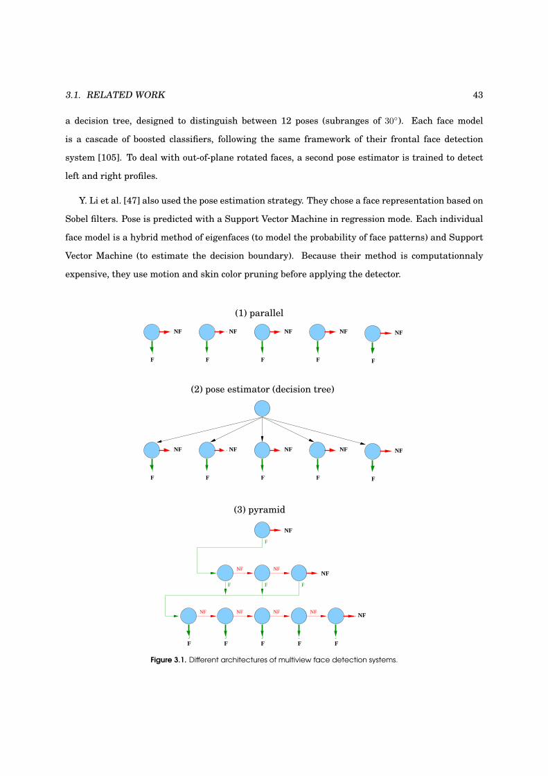
3.1. RELATED WORK 43
a decision tree, designed to distinguish between 12 poses (subranges of 30). Each face model
is a cascade of boosted classifiers, following the same framework of their frontal face detection
system [105]. To deal with out-of-plane rotated faces, a second pose estimator is trained to detect
left and right profiles.
Y. Li et al. [47] also used the pose estimation strategy. They chose a face representation based on
Sobel filters. Pose is predicted with a Support Vector Machine in regression mode. Each individual
face model is a hybrid method of eigenfaces (to model the probability of face patterns) and Support
Vector Machine (to estimate the decision boundary). Because their method is computationnaly
expensive, they use motion and skin color pruning before applying the detector.
F
NF
F
NF
F
NF
F
NF
F
NF
F
NF
F
NF
F
NF
F
NF
F F FF
NF
NF
F F F
F
NF NF
NF NF NF NF
F
NF
F
NF
(2) pose estimator (decision tree)
(3) pyramid
(1) parallel
Figure 3.1. Different architectures of multiview face detection systems.

44 CHAPTER 3. MULTIVIEW FACE DETECTION
S. Li and Zhang [46] introduced the pyramid architecture. Their system, reported as the first
real-time multiview face detection system, is based on an extended set of Haar-like features and on
a new boosting algorithm called FloatBoost. Their pyramid consists of 13 detectors distributed on
three levels. The detector of the top level deals with the full [−90; +90] out-of-plane range. This
range is partitioned into three subranges in the second level, and each subrange is again partitioned
three times in the third level. Each detector is robust to ±15 in-plane rotation. To increase the
in-plane range to ±45, the pyramid detector is applied on the original image as well as on two ±30
in-plane rotated images.
Wu et al. [107] proposed an improved version of the detector of Viola and Jones. RealAdaBoost
is used to train the cascades, composed of lookup tables of Haar-like features. They also remarked
that successive layers in the cascade are loosely correlated and suggested a nested structure where
the output of a given layer is used as the first weak classifier of the next layer. The in-plane range
is partitioned in 12 views and the out-of-plane range in 5 views. Wu et al. also chose the pose
estimation strategy. To predict the orientation, they computed the first six layers of each cascade
and selected the best score. Their method is thus an hybrid version of parallel and pose estimation
strategy.
Huang et al. [34] proposed a novel tree-structured detector. Again, the full range of views is
partitioned in smaller and smaller subranges. They explained that the pyramid architecture treats
all faces as a single class (a sample has to be sent to all the classifiers of the next level), which slows
down the detection process. They also pointed out that in the decision tree architecture, a node
works as a pose estimator and has to select one branch, which may result in a loss in accuracy. In
their proposed tree approach, each branching node is trained with a multiclass version of AdaBoost
which outputs a vector of binary values instead of a single value. Thus, there is no exclusive path
like for a decision tree. A sample may be sent to more than one child node. If all values of the
decision vector are equal to zero, the process stops and the sample is rejected. Huang et al. showed
significant improvements in both accuracy and speed and is currently one of the most effective
multiview face detectors.

3.2. PROPOSED MULTIVIEW FACE DETECTION SYSTEM 45
3.2 Proposed Multiview Face Detection System
Most of the previous approaches are based on the pose prediction strategy. While very fast, these
approaches fully rely on the pose estimator which may affect the accuracy of the detector. The
pyramid approach of Li and Zhang [46] does not focus on the diversity between face poses, but
consider all poses as the same class and try to separate them from nonfaces. This method is more
accurate but also slower. In this section, we propose an improved version of the pyramid detector
of Li and Zhang, which takes advantage of both the pose estimator and the pyramid architectures.
3.2.1 Multiview Face Detector
Our multiview face detector is designed to handle out-of-plane face rotations in the range of [−90; +90]
and in-plane face rotations in the range of [−67.5; +67.5]. The detector architecture, illustrated
in Figure 3.2, is composed of two levels. The top-level detector is trained with all views to quickly
reject as many nonfaces as possible. The second level consists of two modules: one to deal with out-
of-plane rotations and another one to deal with in-plane rotations. The face space is divided into 7
subspaces in the in-plane case and into 9 subspaces in the out-of-plane case, as shown in Fig. 3.3.
If a sample is not rejected by the top-level classifier, it goes through both modules of the second
level. At the top of both modules of the second level, a classifier, called a router, evaluates the sam-
Figure 3.2. Overview of the architecture of the multiview face detector.
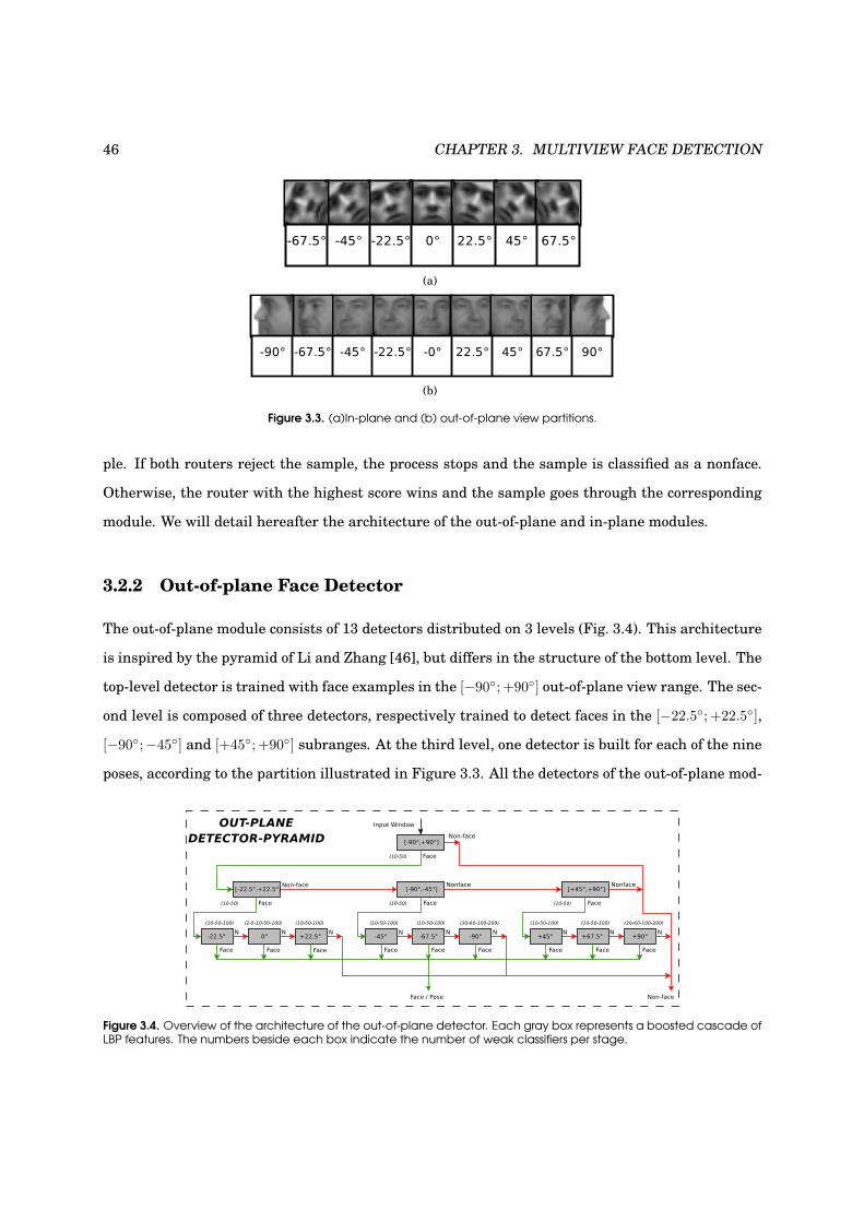
46 CHAPTER 3. MULTIVIEW FACE DETECTION
(a)
(b)
Figure 3.3. (a)In-plane and (b) out-of-plane view partitions.
ple. If both routers reject the sample, the process stops and the sample is classified as a nonface.
Otherwise, the router with the highest score wins and the sample goes through the corresponding
module. We will detail hereafter the architecture of the out-of-plane and in-plane modules.
3.2.2 Out-of-plane Face Detector
The out-of-plane module consists of 13 detectors distributed on 3 levels (Fig. 3.4). This architecture
is inspired by the pyramid of Li and Zhang [46], but differs in the structure of the bottom level. The
top-level detector is trained with face examples in the [−90; +90] out-of-plane view range. The sec-
ond level is composed of three detectors, respectively trained to detect faces in the [−22.5; +22.5],
[−90;−45] and [+45; +90] subranges. At the third level, one detector is built for each of the nine
poses, according to the partition illustrated in Figure 3.3. All the detectors of the out-of-plane mod-
Figure 3.4. Overview of the architecture of the out-of-plane detector. Each gray box represents a boosted cascade ofLBP features. The numbers beside each box indicate the number of weak classifiers per stage.

3.2. PROPOSED MULTIVIEW FACE DETECTION SYSTEM 47
ule are boosted cascades of LBP. For each detector, the number of stages as well as the number of
weak classifiers per stages are given in Fig. 3.4. These values have been chosen empirically. The
same training procedure used for frontal face detection and described in Section 2.2 is applied to
train these detectors.
Let us explain the path taken by a testing sample through the module. First, the sample is
processed by the top-level detector, designed to quickly reject nonfaces. If classified as a face, the
sample goes to the second level. The sample is sent to the third level if one detector of the second
level classifies it as a face; otherwise, the next classifier of the second level is applied. Detectors of
this level may be seen as decision tree nodes, because if accepted as a face, the sample is not sent to
all children node detectors but a subset of three of them. At the third level, the sample is processed
by at most the three detectors of the selected subset, but it is classified as a face as soon as one
detector accepts it. The pose of the sample corresponds to the view of the detector which classified
the sample as a face.
3.2.3 In-plane Face Detector
Instead of rotating the image to handle in-plane rotations like in [46] or [86], we use an architecture
similar to the out-of-plane detector. The in-plane module consists of 8 detectors distributed on 2
levels (Fig. 3.5). The top-level detector is trained with face examples covering the [−67.5; +67.5] in-
plane view range. At the second level, the range is divided into 7 views, according to the partitions
of Fig. 3.3 and one detector is independently trained for each view. As for the out-of-plane module,
all the detectors are trained with the boosting procedure described in Section 2.2. If a sample is not
rejected by the top-level detector, it sequentially goes through the detectors of the second level until
Figure 3.5. Overview of the architecture of the in-plane detector. Each gray box represents a boosted cascade of LBPfeatures. The numbers beside each box indicate the number of weak classifiers per stage.

48 CHAPTER 3. MULTIVIEW FACE DETECTION
one detector classifies it as a face. Again, the pose of the sample is identified by the detector which
accepts the sample as a face.
3.3 Experimental Setup
3.3.1 Training Data
The top-level detector of the multiview pyramid-cascade was trained with faces covering the [−90; +90]
out-of-plane range and the [−67.5; +67.5] in-plane range. Let us describe it in more details.
Out-of-plane Training Data
Our multiview face detector is designed to handle out-of-plane face rotations in the range of [−90; +90].
This range is partitioned in 9 subranges. 4700 face samples from Feret [78], PIE [96] and Prima
Head Pose [26] databases were collected to create the +22.5, +45, +67.5 and +90 face sets. The
faces were mirrored to create the −22.5, −45, −67.5 and −90 face sets. Each face was manually
labelled, cropped according to a face model specific to each pose and subsampled to the size of 19x19
pixels. 15 virtual samples were added from each training face by slightly shifting, scaling, rotating
and mirroring the original sample, leading to a set of about 16000 training samples per pose. These
8 face training sets were used to train the 8 bottom detectors of the out-of-plane detector-pyramid
(the 9th detector is the frontal face detector). The 3 second-level detectors were trained with faces
respectively covering the view ranges of [−22.5; +22.5], [−90;−45] and [+45; +90]. A selection
of faces in the full range of [−90; +90] were used to train the top-level detector.
In-plane Training Data
Our multiview face detector is designed to handle in-plane face rotations in the range of [−67.5; +67.5].
This range is partitioned in 7 subranges. Each face set was created by rotating the training set used
for frontal face detection, respectively by −67.5, −45, −22.5, +22.5, +45, and +67.5. These 6
face training sets were used to train the 6 bottom detectors of the in-plane detector-pyramid (the
7th detector is the frontal face detector). The top-level detector was trained with a selection of faces
covering the full [−67.5; +67.5] in-plane range.

3.3. EXPERIMENTAL SETUP 49
Nonface Training Data
As for the frontal face detection system, nonfaces have been collected by scanning several hundreds
of images containing no face, potentially providing billions of nonface samples. This huge set has
been used to train all detectors of the multiview pyramid-cascade.
3.3.2 Benchmark Test Sets
CMU Rotated Test Set
This data set contains 50 gray-scale images with a total of 223 faces, of which 207 are rotated in
the [−67.5; +67.5] in-plane range. This set was collected by Rowley at CMU [86].
CMU Profile Test Set
This data set consists of 208 images with 441 faces of which 347 are profile views. They were
collected from various news Web sites at CMU by Schneiderman and Kanade [94].
Web and Cinema
These two sets were collected by Garcia and Delakis [24]. The Web test set contains 215 images with
499 faces. The images come from a large set of images that have been submitted to the interactive
demonstration of their system, available on the Web. The Cinema test set consists of 162 images
with 276 faces in challenging conditions (facial expressions, occlusion, complex background).
Sussex
This face database was collected by Jonathan Howell at the University of Sussex. It is composed
of 10 individuals with 10 orientations in the range of [0; +90], leading to a total of 100 gray-scale
images with 100 faces. The faces are surrounded by a simple background. This database can be
freely downloaded from: http://www.cogs.susx.ac.uk/users/jonh/.
3.3.3 Image Scanning
As for frontal face detection, the detector scans the test image at multiple locations and scales.
At each position, the subwindow is evaluated by the detector and classified as either a face or a

50 CHAPTER 3. MULTIVIEW FACE DETECTION
nonface. If it is a face, the detector also provides the pose of the face, which is important for the
overlapped detection merging step.
3.3.4 Merging Overlapped Detections
In Section 2.4.4, we explained that multiple detections at different locations and scales may occur
around faces or face-like regions in the image. The same behavior happens for multiview face
detection. Moreover, these multiple detections may occur for several face poses. Merging overlapped
detections of different poses, like a −22.5 in-plane detection and a +45 out-of-plane detection,
would not make much sense. Hence, we propose the following method, illustrated in Figure 3.6, to
merge multiview overlapped detections:
Figure 3.6. Merging overlapped multiview detections. First, patterns which belongs to the same pose are merged.Then, when several patterns from different poses overlap we choose the one with the highest score.
1. merging per pose: for each pose, detections are merged using the method described in Sec-
tion 2.4.4 for frontal faces. The method consists in a clustering step followed by a merging
step using a detection averaging strategy.
2. final merging: after pose-wise, a clustering step is applied to check whether merged detec-
tions overlap. If it happens, the merged detection with the highest confidence score wins.
The method is illustrated in Figure 3.7. Image (a) shows all the detections of the multiview face
detector (multiple detections for several poses). The merging-per-pose step is applied and the re-
sulting merged detections per pose are displayed on image (b). Multiple detections appear around
some faces, meaning that these faces have been detected by several detectors of different poses. The
best-win merging strategy is applied for each cluster and final detections are drawn in image (c).
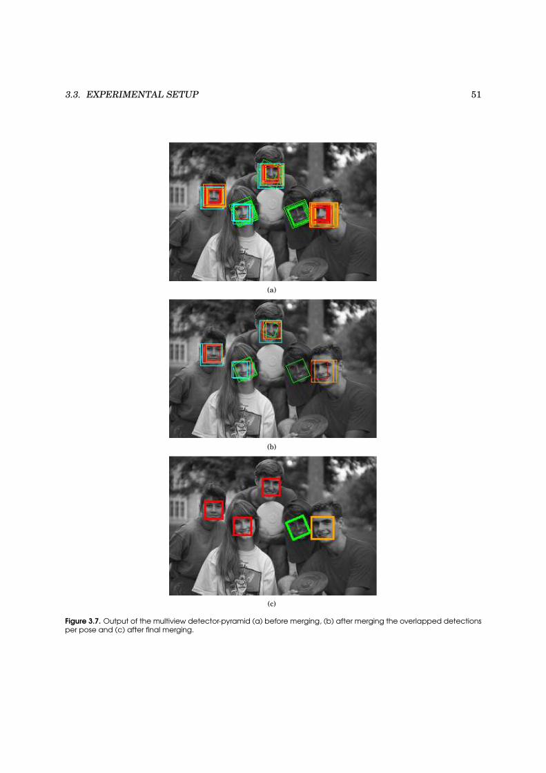
3.3. EXPERIMENTAL SETUP 51
(a)
(b)
(c)
Figure 3.7. Output of the multiview detector-pyramid (a) before merging, (b) after merging the overlapped detectionsper pose and (c) after final merging.
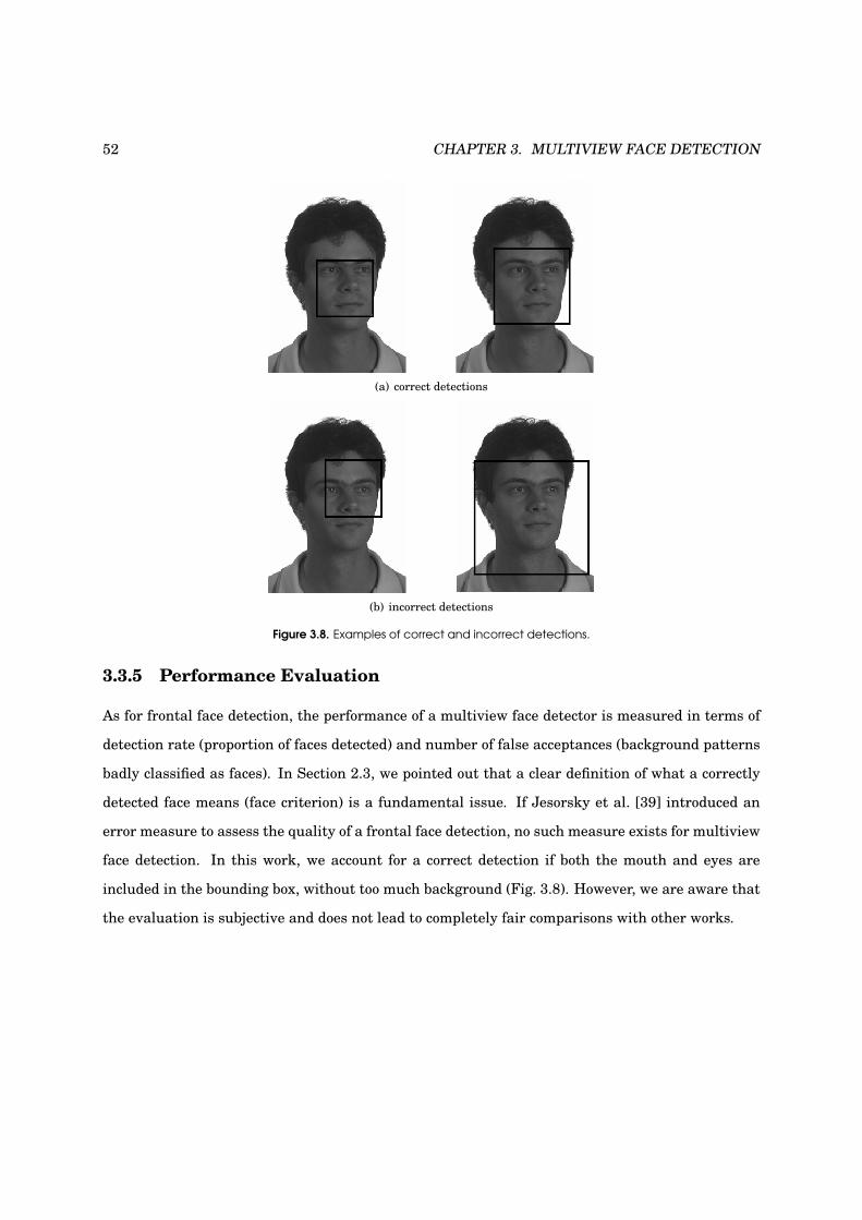
52 CHAPTER 3. MULTIVIEW FACE DETECTION
(a) correct detections
(b) incorrect detections
Figure 3.8. Examples of correct and incorrect detections.
3.3.5 Performance Evaluation
As for frontal face detection, the performance of a multiview face detector is measured in terms of
detection rate (proportion of faces detected) and number of false acceptances (background patterns
badly classified as faces). In Section 2.3, we pointed out that a clear definition of what a correctly
detected face means (face criterion) is a fundamental issue. If Jesorsky et al. [39] introduced an
error measure to assess the quality of a frontal face detection, no such measure exists for multiview
face detection. In this work, we account for a correct detection if both the mouth and eyes are
included in the bounding box, without too much background (Fig. 3.8). However, we are aware that
the evaluation is subjective and does not lead to completely fair comparisons with other works.

3.4. MULTIVIEW FACE DETECTION RESULTS 53
3.4 Multiview Face Detection Results
In this section, some examples of images with detected faces are included. Table 3.1 gives the color
code we use to differentiate the face poses.
Table 3.1. Bounding box color codes to differentiate face poses.Frontal
Bounding Box Color Pose
Red 0
In-plane
Bounding Box Color Pose
Green −67.5, −45, −22.5
Yellow +22.5, +45, +67.5
Out-of-plane
Bounding Box Color Pose
Seagreen −90
Orange −67.5, −45, −22.5
Cyan +22.5, +45, +67.5
Blue +90
3.4.1 Multiview Detector vs. Frontal Detector
Table 3.2 compares the detection rate and the number of false alarms between the baseline frontal
face detector and the multiview face detector, on the CMU-MIT Frontal Test Set (Section 2.4.2).
The proposed system achieves a significantly higher detection rate (91.7%) than the frontal detector
(84.6%) with a similar number of false alarms. Indeed, even though the CMU-MIT set contains only
frontal faces, some of them can be slightly rotated in-plane or out-of-plane (see Fig. 3.9 for some
examples). The multiview face detector is by definition more robust to variation in orientation and
pose, but on the other hand it is also twice as slow.
Table 3.2. Detection rate (DR) and number of false alarms (FA) for our frontal and multiview face detectors on theCMU-MIT Frontal Test Set.
System
CMU Frontal Test Set
DR FA
Baseline Frontal Face Detector84.6% 435
Multiview Face Detector91.7% 441
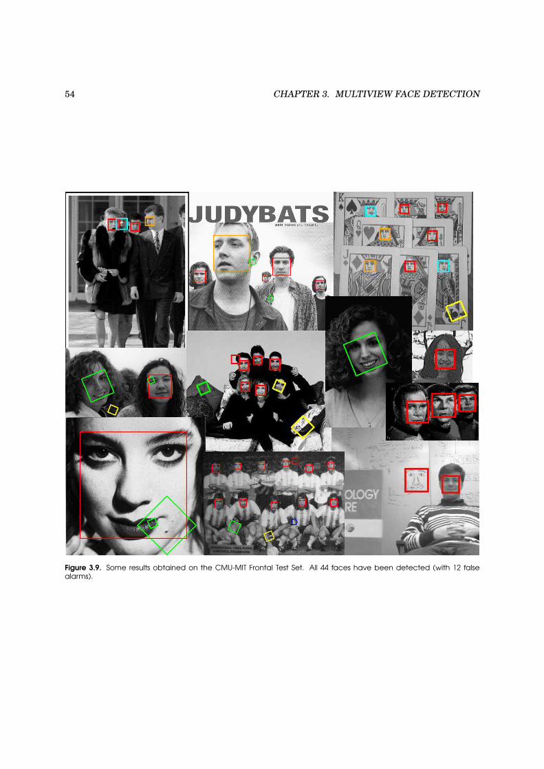
54 CHAPTER 3. MULTIVIEW FACE DETECTION
Figure 3.9. Some results obtained on the CMU-MIT Frontal Test Set. All 44 faces have been detected (with 12 falsealarms).

3.4. MULTIVIEW FACE DETECTION RESULTS 55
3.4.2 In-plane and Out-of-plane Face Detection Results
Table 3.3 compares the detection rate and the number of false alarms between the multiview face
detector and two state-of-the art detectors on the CMU Rotated Test Set and the CMU Profile Test
Set.
Our multiview face detector achieves a higher detection rate (92.3%) than Viola and Jones de-
tector (89.7%), but with a higher number of false alarms. Viola and Jones trained their detector to
detect 12 different poses covering the full 360 in-plane range, whereas our multiview face detec-
tor was trained to detect 16 different poses in-plane and out-of-plane, covering only 135 in-plane.
Thus, the results can not fairly be compared since both detectors are not trained to detect the same
types of faces. Some examples are presented in Fig. 3.10.
Our multiview face detector achieves a much lower detection rate (53.1%) than Schneiderman
and Kanade detector (92.8%) with a lower number of false alarms. The low performance of our
multiview face detection system on this test set can have several reasons. First, Schneiderman and
Kanade trained their detector to cover the full 180 out-of-plane range, when our multiview face
detector also detects faces in the [−67.5; +67.5] in-plane range. Moreover, their detector only dis-
tinguishes frontal, from left or right profile, whereas the proposed system estimates the pose more
precisely: 16 poses are tested where Schneiderman and Kanade only test 3 poses. Furthermore,
Table 3.3. Multiview face detection rate (DR) and number of false alarms (FA) for our multiview face detector and twobaseline detectors on (a) CMU Rotated Test Set and (b) CMU Profile Test Set.
(a)
SystemCMU Rotated Test Set
DR FA
Multiview Face Detector
(in-plane and out-plane)92.3% 342
Viola and Jones [105]
(in-plane only)89.7% 221
(b)
SystemCMU Profile Test Set
DR FA
Multiview Face Detector
(in-plane and out-plane)53.1% 416
Schneiderman and Kanade [94]
(out-plane only)92.8% 700
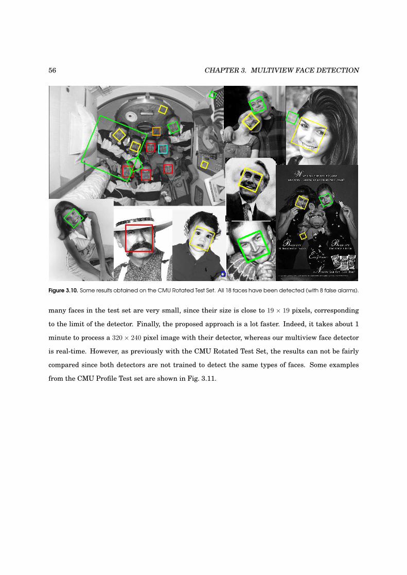
56 CHAPTER 3. MULTIVIEW FACE DETECTION
Figure 3.10. Some results obtained on the CMU Rotated Test Set. All 18 faces have been detected (with 8 false alarms).
many faces in the test set are very small, since their size is close to 19 × 19 pixels, corresponding
to the limit of the detector. Finally, the proposed approach is a lot faster. Indeed, it takes about 1
minute to process a 320 × 240 pixel image with their detector, whereas our multiview face detector
is real-time. However, as previously with the CMU Rotated Test Set, the results can not be fairly
compared since both detectors are not trained to detect the same types of faces. Some examples
from the CMU Profile Test set are shown in Fig. 3.11.
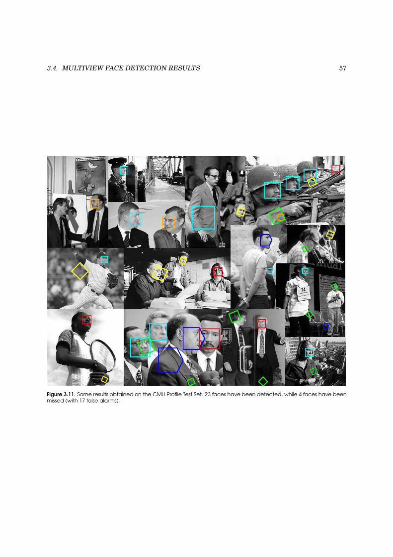
3.4. MULTIVIEW FACE DETECTION RESULTS 57
Figure 3.11. Some results obtained on the CMU Profile Test Set. 23 faces have been detected, while 4 faces have beenmissed (with 17 false alarms).

58 CHAPTER 3. MULTIVIEW FACE DETECTION
3.4.3 Multiview Face Detection Results
Table 3.4 compares the detection rate and the number of false alarms between the multiview face
detector and the one proposed by Garcia and Delakis [24] on the Web and Cinema Test Sets. Both
detectors are multiview detectors, by contrast to Viola and Jones and Schneiderman and Kanade
detectors. This allows a better comparison. Our multiview face detector achieves a lower detection
rate on the Web Test Set (94%) when compared to Garcia and Delakis detector (98%), but a similar
detection rate on the Cinema Test Set (95.3%). On both test sets, our multiview face detector
obtains many more false alarms. However, Garcia and Delakis trained their detector on [−20; +20]
in-plane and [−60; +60] out-of-plane. The view range covered is thus narrower than with our
multiview detector, since the proposed system covers [−67.5; +67.5] in-plane and [−90; +90] out-
of-plane. Moreover, they do not estimate the pose and our system is faster. Fig. 3.12 shows some
results obtained on these test sets.
Table 3.4. Multiview face detection rate (DR) and number of false alarms (FA) for our multiview face detector andGarcia and Delakis detector on Web and Cinema Test Sets.
SystemWeb
DR FA
Cinema
DR FA
Multiview Face Detector 94% 743 95.3% 682
Garcia and Delakis [24] 98% 108 95.3% 104
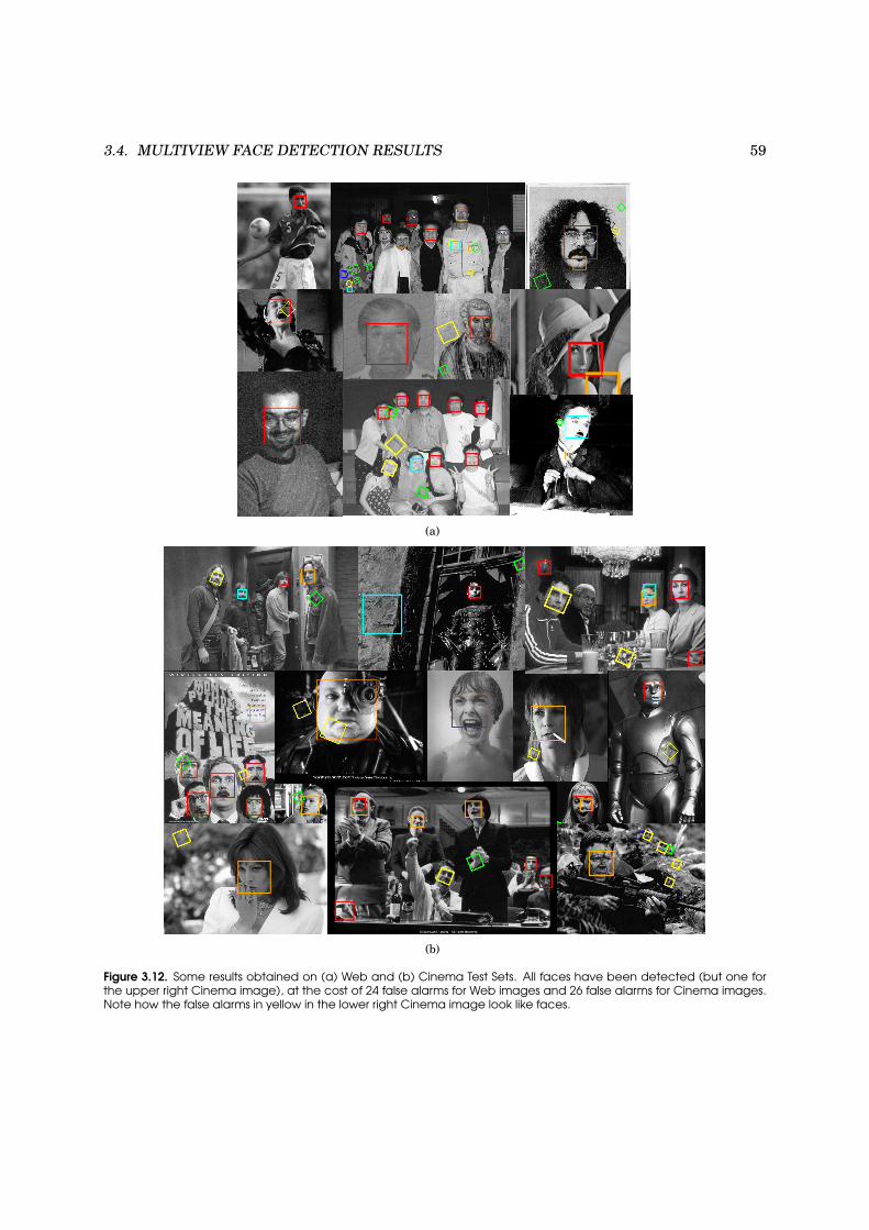
3.4. MULTIVIEW FACE DETECTION RESULTS 59
(a)
(b)
Figure 3.12. Some results obtained on (a) Web and (b) Cinema Test Sets. All faces have been detected (but one forthe upper right Cinema image), at the cost of 24 false alarms for Web images and 26 false alarms for Cinema images.Note how the false alarms in yellow in the lower right Cinema image look like faces.

60 CHAPTER 3. MULTIVIEW FACE DETECTION
3.4.4 Pose Estimation
For each detection, the multiview face detector also estimates the pose. The pose estimation is
evaluated on the Sussex face database (Fig. 3.13). However, only the estimation of the out-of-plane
pose can be evaluated on this database, since it only contains faces rotated out of the image plane.
The 100 images were mirrored (Fig. 3.13 (b)) in order to obtain faces covering the [−90; +90] out-
of-plane view range, leading to a total of 200 images with 10 images per pose (20 for the frontal
pose). The system achieves a detection rate of 98.5% with 10 false alarms and approximately 75%
of the poses which are correctly estimated. Table 3.5 details the number of detections per pose and
gives the percentage of correctly estimated poses. The pose of a face is correctly estimated if the
difference between its angle and the one given by the detector does not exceed +22.5. As each
bottom detector of the detector-pyramid is trained to be robust to pose variations, the ranges that
they cover overlap. Thus, the poses between ±60 and ±30 are those where there are most of the
errors.
Table 3.5. Out-of-plane pose estimation on Sussex Face Database. The bold numbers correspond to the posesconsidered as correctly estimated.
Number of correct detections / detector view Correct
Pose -90˚ -67.5˚ -45˚ -22.5˚ 0˚ 22.5˚ 45˚ 67.5˚ 90˚ Pose Estimation
-90˚ 10 - - - - - - - - 100%
-80˚ 9 1 - - - - - - - 100%
-70˚ 6 2 1 - - - - - - 80%
-60˚ 5 3 1 1 - - - - - 40%
-50˚ 2 3 4 - 1 - - - - 70%
-40˚ - 1 4 3 1 - - - - 70%
-30˚ - 1 4 1 4 - - - - 50%
-20˚ - 1 1 1 7 - - - - 80%
-10˚ - - - 1 9 - - - - 100%
0˚ - - 1 1 16 1 1 - - 90%
10˚ - - - 1 7 - 2 - - 70%
20˚ - - - - 6 2 2 - - 80%
30˚ - - - - 6 - 4 - - 40%
40˚ - - - - 2 - 6 1 1 60%
50˚ - - - - 1 - 1 5 3 60%
60˚ - - - - - - 2 4 4 60%
70˚ - - - - - - 1 1 8 90%
80˚ - - - - - - 1 1 8 90%
90˚ - - - - - - - - 9 90%
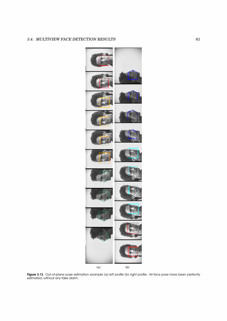
3.4. MULTIVIEW FACE DETECTION RESULTS 61
(a) (b)
Figure 3.13. Out-of-plane pose estimation example (a) left profile (b) right profile. All face pose have been perfectlyestimated, without any false alarm.

62 CHAPTER 3. MULTIVIEW FACE DETECTION
3.5 Conclusion
In this chapter, we extended the frontal face detection system described in Chapter 2 in order to
deal with faces rotated in-plane and out-of-plane. We proposed a novel architecture based on an
improved version of the pyramid detector of Li and Zhang [46]. The system is designed to detect
rotated faces in [−90; +90] out-of-plane range and [−67.5; +67.5] in-plane range. As for frontal
faces, the multiview detector is based on the boosting of LBP features which have shown to be
robust to illumination changes. We showed that the proposed system achieves high performance on
benchmark test sets, comparable to some state-of-the art approaches. The systems handles 16 face
poses, but it is only twice slower than the frontal face detector, and can thus work in real-time.
One limitation of our system is the number of false acceptances. We see two main directions
to cope with this limitation. First, a post-processing stage could be added to reject most false
alarms while keeping a high detection rate. This stage should use another feature space. This
step would however slow down the detection process. Second, the overlapped detections merging
strategy could be improved. Instead of first merging per pose and then applying a best-win strategy
to the resulting overlapped detections, a more relaxed constraint may be considered. For instance,
if a subwindow is classified as a face for pose α, one could consider the score (confidence) of the two
detector adjacent to detector α. This information may help to reject false alarms.
Real-time frontal face detection in controlled conditions (simple background, uniform lighting)
is well solved. Facial expressions, partial occlusions (glasses) or small pose variations around the
frontal pose should also be handled, providing the face appearance variability has been introduced
in the training set. For unconstrained conditions (bad lighting, cluttered background), current
systems still achieve good enough performance for many practical applications.
However, multiview face detection is still a challenging topic, even in controlled scenarios and
especially if real-time is needed. Face appearance variability due to lighting or facial expression
is even larger for profile views than for frontal view. Furthermore, most current algorithms rely
on a pose estimation strategy which is a difficult task in itself and produces many false alarms. If
a precise head pose estimation is required, other techniques, such as particle filtering [2] could be
employed. However, they do not work in real-time. In conclusion, more research is still needed in
order to achieve robust multiview face detection.
Chapter 4
Face Verification Using Adapted
Local Binary Pattern Histograms
Face verification is the second module of the automatic face verification system illustrated in Fig. 1.1.
In this chapter, we propose a novel generative approach for face verification, based on a Local Bi-
nary Pattern (LBP) description of the face. A generic face model is considered as a collection of
LBP-histograms. A client-specific model is then obtained by an adaptation technique from this
generic model under a probabilistic framework. We compare the proposed approach to standard
state-of-the-art face verification methods on two benchmark databases. We also compare our ap-
proach to two state-of-the-art LBP-based face recognition techniques, that we have adapted to the
verification task.
This chapter is organized as follows. First, we review some previous approaches to the face
verification task (Section 4.1) and then introduce a new generative method based on the maximum
a posteriori adaptation of local feature histograms (Section 4.2). Performance evaluation for face
verification and benchmark databases with their protocol are also presented (Section 4.3). We
then compare the proposed approach to state-of-the-art face verification methods, for manual and
automatic face localization (Section 4.4). Finally, we give some concluding remarks and discuss
some possible future ideas (Section 4.5).
63

64CHAPTER 4. FACE VERIFICATION USING ADAPTED LOCAL BINARY PATTERN HISTOGRAMS
4.1 Related Work
A face verification system involves confirming or denying the identity claimed by a person (one-
to-one matching). In the verification mode, people are supposed to cooperate with the system (the
claimant wants to be accepted). The main applications are access control systems, such as computer
log-in, building gate control or digital multimedia access. Face verification has been widely studied
and is performing well in controlled lighting environment and on frontal faces. In real-world ap-
plications (unconstrained environment and non-frontal faces), face verification does not yet achieve
efficient results. Besides the pose of the subject, a major difficulty comes from the appearance vari-
ability of a given identity due to facial expressions, lighting, facial features (mustaches, glasses,
make-up or other artefacts) or even the hair cut and skin color. As depicted in Fig. 1.1, the face
verification module is composed of two steps: feature extraction and feature classification.
4.1.1 Feature Extraction
The main challenge of face verification is to find relevant facial features which best discriminate
individuals, but are robust to intra-personal face appearance variability. In order to allow fast
processing, features should also be easy and fast to extract. Many features have been proposed for
face verification. Among them, we can distinguish holistic and local facial representation.
Holistic facial representation: Holistic approaches consider the face as a whole and repre-
sent it by a single feature vector. The most popular methods include Principal Component Analysis
(PCA) [101] and its extensions (for instance dual PCA [69] or probabilistic PCA [100]), Indepen-
dent Component Analysis (ICA) [4] and Linear Discriminant Analysis (LDA) [52]. Some works do
not perform dimensionality reduction and directly rely on pixel values [58]. Holistic approaches
also include methods which locally extract features in block regions, such as DCT [12], but which
then concatenate all block features in one single high dimensional feature vector. Holistic methods
require a rigid face alignment.
Local facial representation: Approaches that decompose the face into an ensemble of block
regions have reported better performance than holistic approaches and have shown a better robust-
ness against partial occlusions [62] and face localization errors (see Chapter 5). Gabor filters [95]
and DCT [91, 11, 53] are the main representative features of local approaches.

4.2. PROPOSED APPROACH 65
4.1.2 Classification
Given the feature representation of a face sample, the classification step aims to compute a score for
the sample and, according to a decision threshold, accept or reject the sample. Similarity measure
methods, such the Normalized Correlation (NC) [48], are the most simple and popular classifiers.
More complex statistical models such as Neural Networks (NN) [57] or Support Vector Machines
(SVM) [42] are also used. NC, NN or SVM are discriminative approaches. For each client, two
training sets are collected: one containing client examples and another one containing examples
of as many other identities as possible. The classifier is trained to best separate both data sets.
The main limitation of these approaches comes from the small amount of available training data
in practice which makes difficult the design of such models. Recently, it has been shown that
generative approaches such as Gaussian Mixture Models (GMMs) [12] and Hidden Markov Models
(HMMs) [71, 10] were more robust to automatic face localization than the above discriminative
methods. A generative approach computes the likelihood of an observation (holistic) or a set of
observations (local) given a client model and a world model. The client model is trained only with
client data, while the world model is built with data from as many other identities as possible.
4.2 Proposed Approach
4.2.1 Face Representation with Local Binary Patterns
The LBP operator and its extensions have been presented in Section 2.2.1. This operator is defined
as an ordered set of binary comparison between the intensity of the center pixel and the pixels in a
defined neighborhood. It is then unaffected by any monotonic gray-scale transformation which pre-
serves the pixel intensity order in a local neighborhood. Due to its texture discriminative property
and its very low computational cost, LBP is becoming very popular in pattern recognition.
In [1], Ahonen proposed a face recognition system based on a LBP representation of the face.
The individual sample image is divided into R small non-overlapping block regions of same size.
Histograms of LBP codes Hr, with r ∈ 1, 2, . . . , R are calculated over each block and then concate-
nated into a single histogram representing the face image.
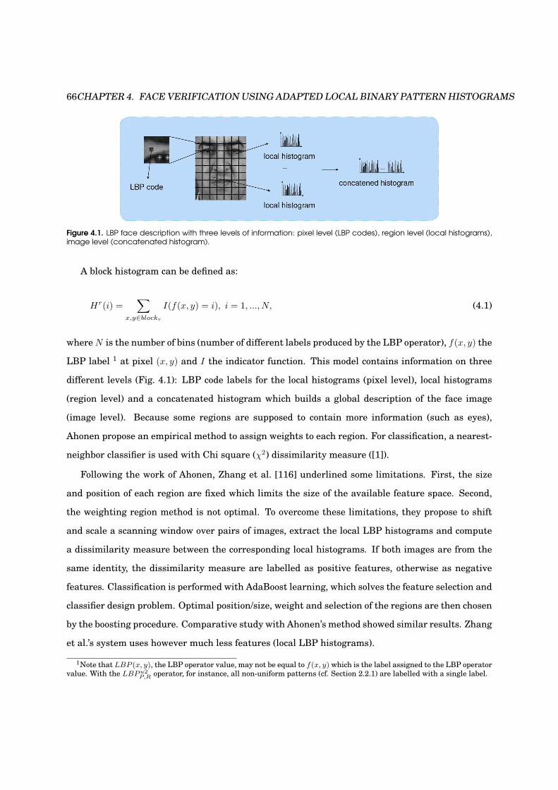
66CHAPTER 4. FACE VERIFICATION USING ADAPTED LOCAL BINARY PATTERN HISTOGRAMS
Figure 4.1. LBP face description with three levels of information: pixel level (LBP codes), region level (local histograms),image level (concatenated histogram).
A block histogram can be defined as:
Hr(i) =∑
x,y∈blockr
I(f(x, y) = i), i = 1, ..., N, (4.1)
where N is the number of bins (number of different labels produced by the LBP operator), f(x, y) the
LBP label 1 at pixel (x, y) and I the indicator function. This model contains information on three
different levels (Fig. 4.1): LBP code labels for the local histograms (pixel level), local histograms
(region level) and a concatenated histogram which builds a global description of the face image
(image level). Because some regions are supposed to contain more information (such as eyes),
Ahonen propose an empirical method to assign weights to each region. For classification, a nearest-
neighbor classifier is used with Chi square (χ2) dissimilarity measure ([1]).
Following the work of Ahonen, Zhang et al. [116] underlined some limitations. First, the size
and position of each region are fixed which limits the size of the available feature space. Second,
the weighting region method is not optimal. To overcome these limitations, they propose to shift
and scale a scanning window over pairs of images, extract the local LBP histograms and compute
a dissimilarity measure between the corresponding local histograms. If both images are from the
same identity, the dissimilarity measure are labelled as positive features, otherwise as negative
features. Classification is performed with AdaBoost learning, which solves the feature selection and
classifier design problem. Optimal position/size, weight and selection of the regions are then chosen
by the boosting procedure. Comparative study with Ahonen’s method showed similar results. Zhang
et al.’s system uses however much less features (local LBP histograms).
1Note that LBP (x, y), the LBP operator value, may not be equal to f(x, y) which is the label assigned to the LBP operator
value. With the LBP u2
P,Roperator, for instance, all non-uniform patterns (cf. Section 2.2.1) are labelled with a single label.

4.2. PROPOSED APPROACH 67
4.2.2 Model Description
In this chapter, we propose a new generative model for face verification, based on a LBP description
of the face. Sample images are divided in R non-overlapping block regions of same size. This block
by block basis is mainly motivated by the success of some recent works [53, 91, 10]. Similar to [1],
a histogram of LBP codes is computed for each block. However, this histogram is not seen as a
static observation. We instead consider it as a probability distribution. Each block histogram is
thus normalized:∑
i Hr(i) = 1, where r ∈ 1, 2, . . . , R.
Given a claim for client C, let us denote a set of independent features X = xrRr=1, extracted
from the given face image. If θC is the set of parameters to be estimated from sample X, we can
define the likelihood of the claim coming from the true claimant C as:
P (X|θC) =
R∏
r=1
p(xr|θC) (4.2)
=
R∏
r=1
p(xr|θC1, . . . , θCR
) (4.3)
=
R∏
r=1
p(xr|θCr), (4.4)
assuming that each block is independent and that θC can be decomposed as a set of independent
parameters per block (θC1, . . . , θCR
).
The next important step consists in choosing the function to estimate the likelihood functions
p(xr|θCr). We chose a very simple and computationally inexpensive non parametric model: his-
togram of LBP codes (Fig. 4.2). xr = lkKk=1 is thus defined as a set of K labelled LBP code
observations, where K is the maximum number of kernels which can be computed in the block by
the LBP operator. This value is constant because all blocks have the same size. Assuming that each
LBP code observation is independent, we can thus develop further:
P (X|θC) =
R∏
r=1
p(xr|θCr) (4.5)
=
R∏
r=1
p(l1, . . . , lK |θCr) (4.6)
=
R∏
r=1
K∏
k=1
p(lk|θCr) (4.7)
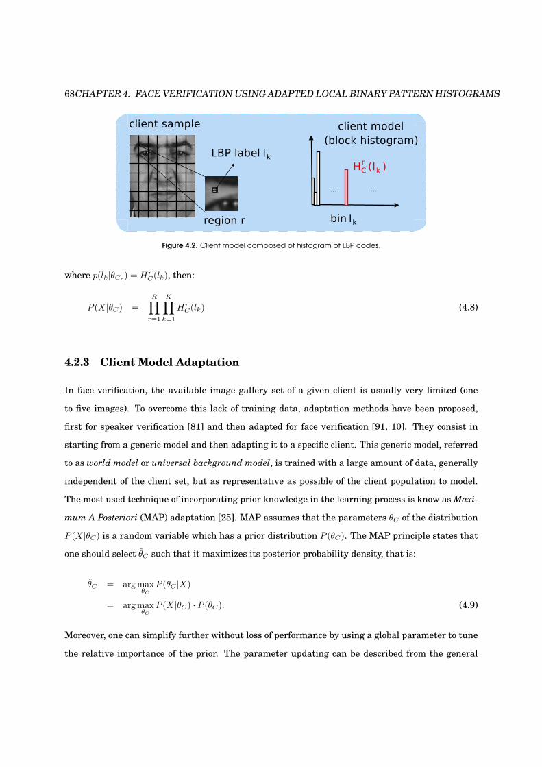
68CHAPTER 4. FACE VERIFICATION USING ADAPTED LOCAL BINARY PATTERN HISTOGRAMS
Figure 4.2. Client model composed of histogram of LBP codes.
where p(lk|θCr) = Hr
C(lk), then:
P (X|θC) =R
∏
r=1
K∏
k=1
HrC(lk) (4.8)
4.2.3 Client Model Adaptation
In face verification, the available image gallery set of a given client is usually very limited (one
to five images). To overcome this lack of training data, adaptation methods have been proposed,
first for speaker verification [81] and then adapted for face verification [91, 10]. They consist in
starting from a generic model and then adapting it to a specific client. This generic model, referred
to as world model or universal background model, is trained with a large amount of data, generally
independent of the client set, but as representative as possible of the client population to model.
The most used technique of incorporating prior knowledge in the learning process is know as Maxi-
mum A Posteriori (MAP) adaptation [25]. MAP assumes that the parameters θC of the distribution
P (X|θC) is a random variable which has a prior distribution P (θC). The MAP principle states that
one should select θC such that it maximizes its posterior probability density, that is:
θC = arg maxθC
P (θC |X)
= arg maxθC
P (X|θC) · P (θC). (4.9)
Moreover, one can simplify further without loss of performance by using a global parameter to tune
the relative importance of the prior. The parameter updating can be described from the general

4.2. PROPOSED APPROACH 69
Figure 4.3. Illustration of the client model adaptation.
MAP estimation equations using constraints on the prior distribution presented in [25]:
HrC(lk) = αHr
W (lk) + (1 − α)HrC(lk) (4.10)
where HrW (lk) is the feature value (bin lk of the histogram of block r) of the world model (prior),
HrC(lk) is the current estimation (client training data) and Hr
C(lk) is the updated feature value
(Fig. 4.3). The weighting factor α is chosen by cross-validation. The client model is thus a combina-
tion of parameters estimated from an independent world model and from training samples. After
adaptation, each block histogram HrC is normalized to remain a probability distribution.
4.2.4 Face Verification Task
Let us denote θC the parameter set for client model C, θW the parameter set for the world model
and a set of feature X. The binary process of face verification can be expressed as follows:
Λ(X) = log P (X|θC) − log P (X|θW ) (4.11)
where P (X|θC) is the likelihood of the claim coming from the true claimant and P (X|θW ) is the
likelihood of the claim coming from an impostor. Given a decision threshold τ , the claim is accepted
when Λ(X) > τ and rejected when Λ(X) < τ . P (X|θ.) is computed using Eq.4.8.
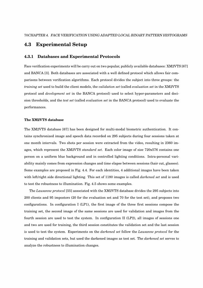
70CHAPTER 4. FACE VERIFICATION USING ADAPTED LOCAL BINARY PATTERN HISTOGRAMS
4.3 Experimental Setup
4.3.1 Databases and Experimental Protocols
Face verification experiments will be carry out on two popular, publicly available databases: XM2VTS [67]
and BANCA [3]. Both databases are associated with a well defined protocol which allows fair com-
parisons between verification algorithms. Each protocol divides the subject into three groups: the
training set used to build the client models, the validation set (called evaluation set in the XM2VTS
protocol and development set in the BANCA protocol) used to select hyper-parameters and deci-
sion thresholds, and the test set (called evaluation set in the BANCA protocol) used to evaluate the
performances.
The XM2VTS database
The XM2VTS database [67] has been designed for multi-modal biometric authentication. It con-
tains synchronized image and speech data recorded on 295 subjects during four sessions taken at
one month intervals. Two shots per session were extracted from the video, resulting in 2360 im-
ages, which represent the XM2VTS standard set. Each color image of size 720x576 contains one
person on a uniform blue background and in controlled lighting conditions. Intra-personal vari-
ability mainly comes from expression changes and time elapse between sessions (hair cut, glasses).
Some examples are proposed in Fig. 4.4. For each identities, 4 additional images have been taken
with left/right side directional lighting. This set of 1180 images is called darkened set and is used
to test the robustness to illumination. Fig. 4.5 shows some examples.
The Lausanne protocol [55] associated with the XM2VTS database divides the 295 subjects into
200 clients and 95 impostors (20 for the evaluation set and 70 for the test set), and proposes two
configurations. In configuration I (LP1), the first image of the three first sessions compose the
training set, the second image of the same sessions are used for validation and images from the
fourth session are used to test the system. In configuration II (LP2), all images of sessions one
and two are used for training, the third session constitutes the validation set and the last session
is used to test the system. Experiments on the darkened set follow the Lausanne protocol for the
training and validation sets, but used the darkened images as test set. The darkened set serves to
analyze the robustness to illumination changes.
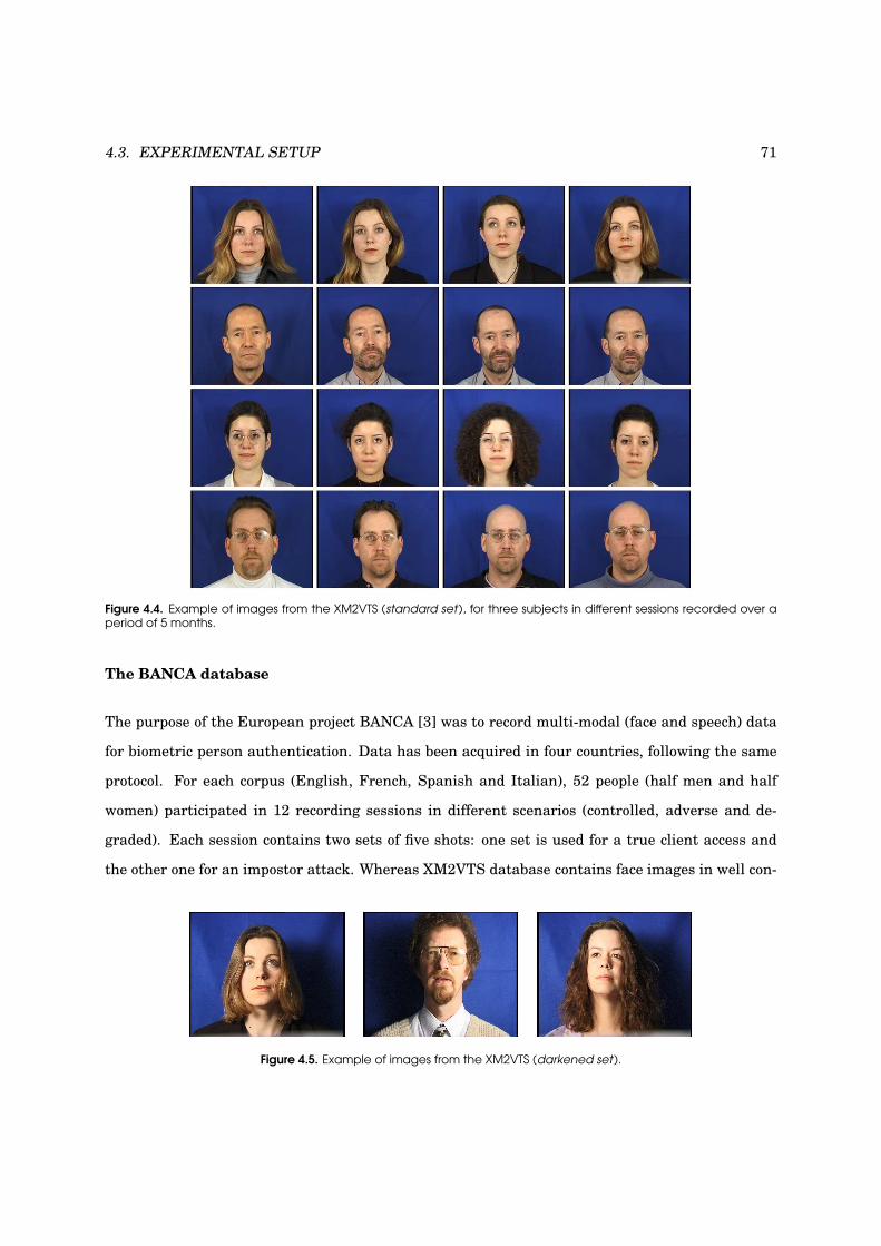
4.3. EXPERIMENTAL SETUP 71
Figure 4.4. Example of images from the XM2VTS (standard set), for three subjects in different sessions recorded over aperiod of 5 months.
The BANCA database
The purpose of the European project BANCA [3] was to record multi-modal (face and speech) data
for biometric person authentication. Data has been acquired in four countries, following the same
protocol. For each corpus (English, French, Spanish and Italian), 52 people (half men and half
women) participated in 12 recording sessions in different scenarios (controlled, adverse and de-
graded). Each session contains two sets of five shots: one set is used for a true client access and
the other one for an impostor attack. Whereas XM2VTS database contains face images in well con-
Figure 4.5. Example of images from the XM2VTS (darkened set).
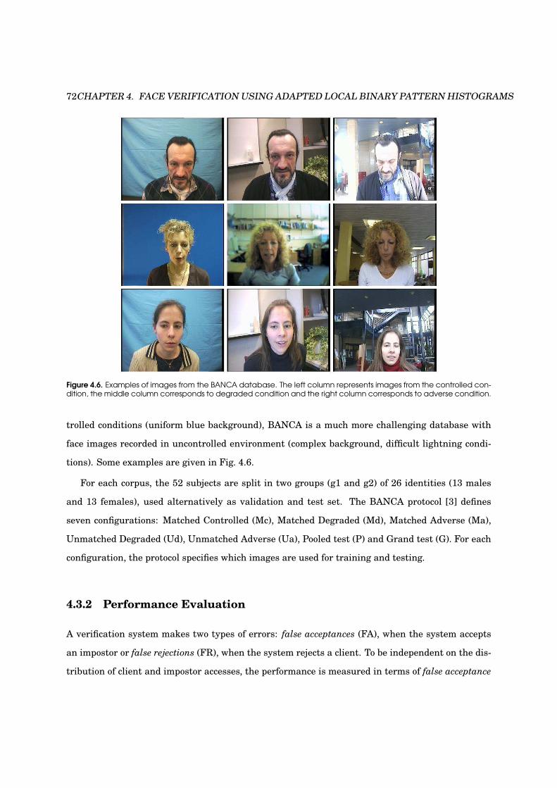
72CHAPTER 4. FACE VERIFICATION USING ADAPTED LOCAL BINARY PATTERN HISTOGRAMS
Figure 4.6. Examples of images from the BANCA database. The left column represents images from the controlled con-dition, the middle column corresponds to degraded condition and the right column corresponds to adverse condition.
trolled conditions (uniform blue background), BANCA is a much more challenging database with
face images recorded in uncontrolled environment (complex background, difficult lightning condi-
tions). Some examples are given in Fig. 4.6.
For each corpus, the 52 subjects are split in two groups (g1 and g2) of 26 identities (13 males
and 13 females), used alternatively as validation and test set. The BANCA protocol [3] defines
seven configurations: Matched Controlled (Mc), Matched Degraded (Md), Matched Adverse (Ma),
Unmatched Degraded (Ud), Unmatched Adverse (Ua), Pooled test (P) and Grand test (G). For each
configuration, the protocol specifies which images are used for training and testing.
4.3.2 Performance Evaluation
A verification system makes two types of errors: false acceptances (FA), when the system accepts
an impostor or false rejections (FR), when the system rejects a client. To be independent on the dis-
tribution of client and impostor accesses, the performance is measured in terms of false acceptance

4.3. EXPERIMENTAL SETUP 73
rate (FAR) and false rejection rate (FRR), defined as follows:
FAR =number of FAs
number of impostor accesses(4.12)
FRR =number of FRs
number of true claimant accesses(4.13)
Generally, the Half Total Error Rate (HTER) is reported to assess the performance of a verification
system:
HTER =FAR + FRR
2(4.14)
However, because FAR and FRR are related (decreasing one means increasing the other), a more
useful measure, called Weighted Error Rate (WER), is used in practice:
WER(τ∗) = ωFAR(τ∗) + (1 − ω) FRR (τ∗) (4.15)
where ω ∈ [0, 1] is set for a specific situation and τ∗ is the threshold that minimizes the WER for a
given ω. This FAR vs. FRR trade-off may be seen as a trade-off between level of security (controlled
by the FAR) and usability (controlled by the FRR). Note that to correspond to a realistic situation,
τ∗ should not be chosen (a posteriori) on the test set, but (a priori) on the validation set.
In order to illustrate the FAR vs. FRR trade-off, the Receiver Operating Characteristics (ROC)
curve [103], which plots FRR as a function of FAR, is often reported in the literature. Sometimes
the Detection Error Tradeoff (DET) [61] curve, which is a non-linear transformation of the ROC
curve, is preferred for easier comparison. Recently, Bengio et al. [7] observed that these curves
can be misleading, because, they do not take into account that, in real life, the threshold has to be
selected a priori. Instead, they propose the Expected Performance Curve (EPC). For each value of ω
in Equation 4.15, the threshold τ∗ is first found on the validation set; the HTER is then found on
the test set and is plotted as a function of ω. The EPC may be seen as an unbiased version of the
ROC curve.
In the following sets of experiments, we will only report HTERs, with the decision threshold
chosen a priori on the validation set at Equal Error Rate (i.e. for FAR = FRR). ROC curves or
EPCs are practically useful to compare systems which have very similar performances, and select
74CHAPTER 4. FACE VERIFICATION USING ADAPTED LOCAL BINARY PATTERN HISTOGRAMS
the best system for a particular operating point.
4.3.3 The Proposed LBP/MAP Face Verification System
For both XM2VTS and BANCA databases, face images are extracted to a size of 84 × 68 (rows ×
columns), according to the eye positions, either provided by the groundtruth (manual localization)
or by a face detection system (automatic localization). The cropped faces are then processed with
the LBPu28,2 operator (N = 59 labels). The resulting 80× 64 LBP face images do not need any further
lighting normalization, due to the gray-scale invariant property of LBP operators. In a block by
block basis, the face images are decomposed in 8 × 8 blocks (R = 80 blocks). Histograms of LBP
codes are then computed over each block r and normalized (∑
i Hr(i) = 1, where i ∈ 1, 2, . . . , N).
For experiments on the XM2VTS database, we use all available training client images to build
the generic model. For BANCA experiments, the generic model was trained with the additional
set of images, referred to as world data (independent of the subjects in the client database). For
all experiments, the adaptation factor α of Eq. 4.10 (client model adaptation) is selected on the
validation set.
For comparison purpose, we implemented the systems of Ahonen [1] and Zhang [116], briefly
described in Section 4.2.1. Similarly, we used a 8 × 8 block decomposition and computed LBP
histograms for each block with the LBPu28,2 operator.
4.4 Face Verification Results
4.4.1 Manual Face Localization
Results on the XM2VTS Database
Table 4.1 reports comparative results for Ahonen and Zhang systems, our proposed LBP/MAP his-
togram adaptation approach, as well as for two standard state-of-the-art methods. LDA/NC, as
described in [66], combines Linear Discriminant Analysis with Normalized Correlation (holistic
representation of the face), while DCT/GMM [12] is a generative approach based on a modified
version of the Discrete Cosine Transform and Gaussian Mixture Models (local description of the
face).
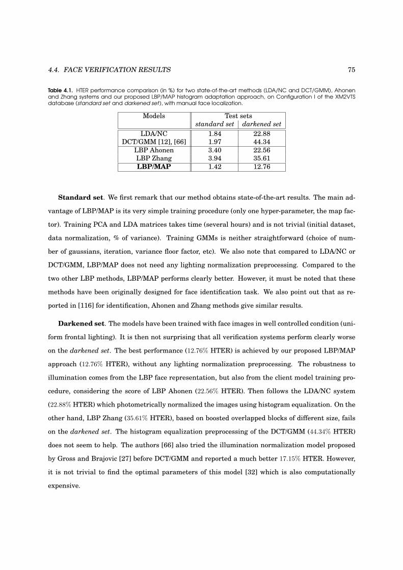
4.4. FACE VERIFICATION RESULTS 75
Table 4.1. HTER performance comparison (in %) for two state-of-the-art methods (LDA/NC and DCT/GMM), Ahonenand Zhang systems and our proposed LBP/MAP histogram adaptation approach, on Configuration I of the XM2VTSdatabase (standard set and darkened set), with manual face localization.
Models Test sets
standard set darkened set
LDA/NC 1.84 22.88
DCT/GMM [12], [66] 1.97 44.34
LBP Ahonen 3.40 22.56
LBP Zhang 3.94 35.61
LBP/MAP 1.42 12.76
Standard set. We first remark that our method obtains state-of-the-art results. The main ad-
vantage of LBP/MAP is its very simple training procedure (only one hyper-parameter, the map fac-
tor). Training PCA and LDA matrices takes time (several hours) and is not trivial (initial dataset,
data normalization, % of variance). Training GMMs is neither straightforward (choice of num-
ber of gaussians, iteration, variance floor factor, etc). We also note that compared to LDA/NC or
DCT/GMM, LBP/MAP does not need any lighting normalization preprocessing. Compared to the
two other LBP methods, LBP/MAP performs clearly better. However, it must be noted that these
methods have been originally designed for face identification task. We also point out that as re-
ported in [116] for identification, Ahonen and Zhang methods give similar results.
Darkened set. The models have been trained with face images in well controlled condition (uni-
form frontal lighting). It is then not surprising that all verification systems perform clearly worse
on the darkened set. The best performance (12.76% HTER) is achieved by our proposed LBP/MAP
approach (12.76% HTER), without any lighting normalization preprocessing. The robustness to
illumination comes from the LBP face representation, but also from the client model training pro-
cedure, considering the score of LBP Ahonen (22.56% HTER). Then follows the LDA/NC system
(22.88% HTER) which photometrically normalized the images using histogram equalization. On the
other hand, LBP Zhang (35.61% HTER), based on boosted overlapped blocks of different size, fails
on the darkened set. The histogram equalization preprocessing of the DCT/GMM (44.34% HTER)
does not seem to help. The authors [66] also tried the illumination normalization model proposed
by Gross and Brajovic [27] before DCT/GMM and reported a much better 17.15% HTER. However,
it is not trivial to find the optimal parameters of this model [32] which is also computationally
expensive.
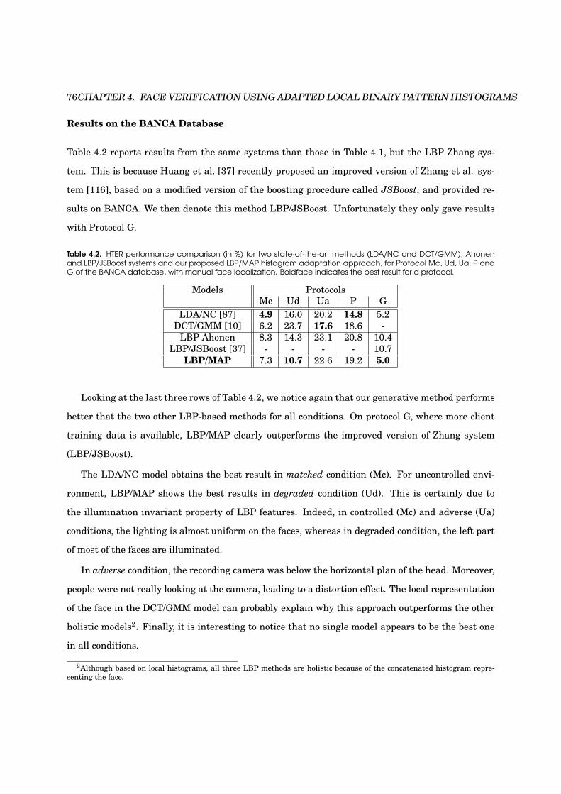
76CHAPTER 4. FACE VERIFICATION USING ADAPTED LOCAL BINARY PATTERN HISTOGRAMS
Results on the BANCA Database
Table 4.2 reports results from the same systems than those in Table 4.1, but the LBP Zhang sys-
tem. This is because Huang et al. [37] recently proposed an improved version of Zhang et al. sys-
tem [116], based on a modified version of the boosting procedure called JSBoost, and provided re-
sults on BANCA. We then denote this method LBP/JSBoost. Unfortunately they only gave results
with Protocol G.
Table 4.2. HTER performance comparison (in %) for two state-of-the-art methods (LDA/NC and DCT/GMM), Ahonenand LBP/JSBoost systems and our proposed LBP/MAP histogram adaptation approach, for Protocol Mc, Ud, Ua, P andG of the BANCA database, with manual face localization. Boldface indicates the best result for a protocol.
Models Protocols
Mc Ud Ua P G
LDA/NC [87] 4.9 16.0 20.2 14.8 5.2
DCT/GMM [10] 6.2 23.7 17.6 18.6 -
LBP Ahonen 8.3 14.3 23.1 20.8 10.4
LBP/JSBoost [37] - - - - 10.7
LBP/MAP 7.3 10.7 22.6 19.2 5.0
Looking at the last three rows of Table 4.2, we notice again that our generative method performs
better that the two other LBP-based methods for all conditions. On protocol G, where more client
training data is available, LBP/MAP clearly outperforms the improved version of Zhang system
(LBP/JSBoost).
The LDA/NC model obtains the best result in matched condition (Mc). For uncontrolled envi-
ronment, LBP/MAP shows the best results in degraded condition (Ud). This is certainly due to
the illumination invariant property of LBP features. Indeed, in controlled (Mc) and adverse (Ua)
conditions, the lighting is almost uniform on the faces, whereas in degraded condition, the left part
of most of the faces are illuminated.
In adverse condition, the recording camera was below the horizontal plan of the head. Moreover,
people were not really looking at the camera, leading to a distortion effect. The local representation
of the face in the DCT/GMM model can probably explain why this approach outperforms the other
holistic models2. Finally, it is interesting to notice that no single model appears to be the best one
in all conditions.
2Although based on local histograms, all three LBP methods are holistic because of the concatenated histogram repre-
senting the face.
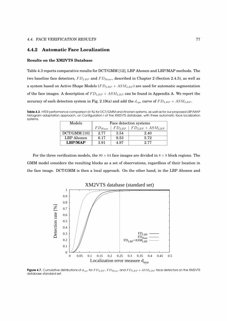
4.4. FACE VERIFICATION RESULTS 77
4.4.2 Automatic Face Localization
Results on the XM2VTS Database
Table 4.3 reports comparative results for DCT/GMM [12], LBP Ahonen and LBP/MAP methods. The
two baseline face detectors, FDLBP and FDHaar, described in Chapter 2 (Section 2.4.5), as well as
a system based on Active Shape Models (FDLBP + ASMLBP ) are used for automatic segmentation
of the face images. A description of FDLBP + ASMLBP can be found in Appendix A. We report the
accuracy of each detection system in Fig. 2.19(a) and add the deye curve of FDLBP + ASMLBP .
Table 4.3. HTER performance comparison (in %) for DCT/GMM and Ahonen systems, as well as for our proposed LBP/MAPhistogram adaptation approach, on Configuration I of the XM2VTS database, with three automatic face localizationsystems.
Models Face detection systems
FDHaar FDLBP FDLBP + ASMLBP
DCT/GMM [10] 2.77 3.54 2.40
LBP Ahonen 6.17 9.53 5.72
LBP/MAP 3.91 4.97 2.77
For the three verification models, the 80 × 64 face images are divided in 8 × 8 block regions. The
GMM model considers the resulting blocks as a set of observations, regardless of their location in
the face image. DCT/GMM is then a local approach. On the other hand, in the LBP Ahonen and
1
0.9
0.8
0.7
0.6
0.5
0.4
0.3
0.2
0.1
0 0.5 0.45 0.4 0.35 0.3 0.25 0.2 0.15 0.1 0.05 0
Det
ectio
n ra
te [
%]
Localization error measure deye
XM2VTS database (standard set)
FDLBPFDHaar
FDLBP+ASMLBP
Figure 4.7. Cumulative distributions of deye for FDLBP , FDHaar and FDLBP +ASMLBP face detectors on the XM2VTSdatabase standard set.
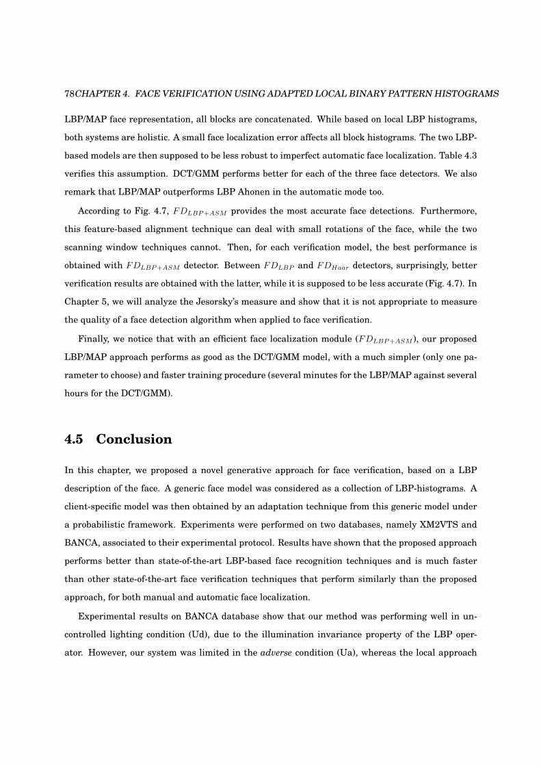
78CHAPTER 4. FACE VERIFICATION USING ADAPTED LOCAL BINARY PATTERN HISTOGRAMS
LBP/MAP face representation, all blocks are concatenated. While based on local LBP histograms,
both systems are holistic. A small face localization error affects all block histograms. The two LBP-
based models are then supposed to be less robust to imperfect automatic face localization. Table 4.3
verifies this assumption. DCT/GMM performs better for each of the three face detectors. We also
remark that LBP/MAP outperforms LBP Ahonen in the automatic mode too.
According to Fig. 4.7, FDLBP+ASM provides the most accurate face detections. Furthermore,
this feature-based alignment technique can deal with small rotations of the face, while the two
scanning window techniques cannot. Then, for each verification model, the best performance is
obtained with FDLBP+ASM detector. Between FDLBP and FDHaar detectors, surprisingly, better
verification results are obtained with the latter, while it is supposed to be less accurate (Fig. 4.7). In
Chapter 5, we will analyze the Jesorsky’s measure and show that it is not appropriate to measure
the quality of a face detection algorithm when applied to face verification.
Finally, we notice that with an efficient face localization module (FDLBP+ASM ), our proposed
LBP/MAP approach performs as good as the DCT/GMM model, with a much simpler (only one pa-
rameter to choose) and faster training procedure (several minutes for the LBP/MAP against several
hours for the DCT/GMM).
4.5 Conclusion
In this chapter, we proposed a novel generative approach for face verification, based on a LBP
description of the face. A generic face model was considered as a collection of LBP-histograms. A
client-specific model was then obtained by an adaptation technique from this generic model under
a probabilistic framework. Experiments were performed on two databases, namely XM2VTS and
BANCA, associated to their experimental protocol. Results have shown that the proposed approach
performs better than state-of-the-art LBP-based face recognition techniques and is much faster
than other state-of-the-art face verification techniques that perform similarly than the proposed
approach, for both manual and automatic face localization.
Experimental results on BANCA database show that our method was performing well in un-
controlled lighting condition (Ud), due to the illumination invariance property of the LBP oper-
ator. However, our system was limited in the adverse condition (Ua), whereas the local approach

4.5. CONCLUSION 79
(DCT/GMM) was performing best. This limitation comes from the holistic representation of the face
(concatenated LBP histograms). The next step would be to relax the constraints on the location of
the blocks and consider a more elastic grid. One promising direction we are investigating is to look
at the close neighborhood of each block and select the region with the highest likelihood.
The experimental section also showed the limitation of the current face detection measure (deye).
FDHaar detector, which was supposed to be less accurate than FDLBP detector according to the deye
measure, actually led to better face verification performance. In the next chapter, we will analyze
the limitation of deye measure in more details.

80CHAPTER 4. FACE VERIFICATION USING ADAPTED LOCAL BINARY PATTERN HISTOGRAMS

Chapter 5
Measuring the Performance of
Face Localization Systems
This chapter concerns the performance evaluation of face localization algorithms. We argue that
a universal performance measure does not exist, because localization errors may have different
impacts depending on the final application for which the localization algorithm has been designed.
We think that the performance measure should be specifically tailored for the final application. In
this chapter, we focus on the face verification task. In that context, the best localization system
should be the one that minimizes the number of errors made by a specific verification system.
First, we start by analyzing how the various types of localization errors (shift, rotation, scale)
affect the performance of two face verification algorithms. This empirical analysis demonstrates
that the different types of localization errors do not induce the same verification error, even if
current localization performance measures would have rated them similarly.
Then, we propose a new localization measure which embeds the final application (here face ver-
ification) into the performance measuring process. This measure estimates directly the verification
errors as a function of the errors made by the localization algorithm. We then empirically show that
the proposed measure better matches the final verification performance.
This chapter is organized as follows. First, we will review classical measures currently used in
the literature to evaluate the performance of a face localization algorithm (Section 5.1). Then, we
81

82 CHAPTER 5. MEASURING THE PERFORMANCE OF FACE LOCALIZATION SYSTEMS
will present two empirical analyses that both show that the performance of a localization algorithm
can only make sense in the context of the application for which the localization algorithm was built
for (Section 5.2). Thus, we propose a new face localization measure which takes into account the
performance of the final application, here face verification (Section 5.3). The idea of the proposed
measure consists in estimating the error made by the verification process given the error made by
the localization process. We provide an empirical evaluation on how performance measure behaves
on a real benchmark database (Section 5.4), and we finally conclude (Section 5.5).
5.1 Performance Measures for Face Localization
5.1.1 Lack of Uniformity
Direct comparison of face localization systems is a very difficult task, mainly because there is no
clear definition of what a good face localization is. While most concerned papers found in the litera-
ture provide localization and error rates, almost none mention the way they count a correct/incorrect
hit that leads to computation of these rates. Furthermore, when reported, the underlying criterion
is usually not clearly described. For instance, in [99] and [36], a detected window is counted as a
true or false detection based on the visual observation that the box includes both eyes, the nose and
the mouth. According to Yang’s survey [111], Rowley et al. [85] adjust the criterion until the exper-
imental results match their intuition of what a correct detection is (i.e. the square window should
contain the eyes and also the mouth). In some rare works, the face localization criterion is more pre-
cisely presented. In [49] for instance, Lienhart et al. count a correct hit if the Euclidean distance
between the centers of the detected and the true face is less than 30% of the width of the true face,
and the width of the detected face is within ±50% of the true face. In [23], the authors consider
a true detection if the measured face position (through the position of the eyes) and size (through
the distance between the eyes) do not differ more than 30% from the true values. Unfortunately,
the lack of uniformity between reported results makes them particularly difficult to compare and
reproduce.
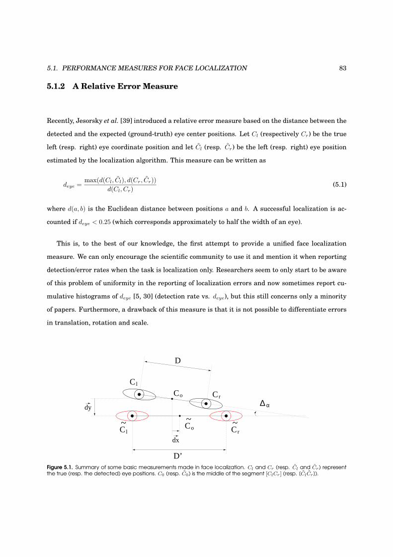
5.1. PERFORMANCE MEASURES FOR FACE LOCALIZATION 83
5.1.2 A Relative Error Measure
Recently, Jesorsky et al. [39] introduced a relative error measure based on the distance between the
detected and the expected (ground-truth) eye center positions. Let Cl (respectively Cr) be the true
left (resp. right) eye coordinate position and let Cl (resp. Cr) be the left (resp. right) eye position
estimated by the localization algorithm. This measure can be written as
deye =max(d(Cl, Cl), d(Cr, Cr))
d(Cl, Cr)(5.1)
where d(a, b) is the Euclidean distance between positions a and b. A successful localization is ac-
counted if deye < 0.25 (which corresponds approximately to half the width of an eye).
This is, to the best of our knowledge, the first attempt to provide a unified face localization
measure. We can only encourage the scientific community to use it and mention it when reporting
detection/error rates when the task is localization only. Researchers seem to only start to be aware
of this problem of uniformity in the reporting of localization errors and now sometimes report cu-
mulative histograms of deye [5, 30] (detection rate vs. deye), but this still concerns only a minority
of papers. Furthermore, a drawback of this measure is that it is not possible to differentiate errors
in translation, rotation and scale.
~Co
Co C r
C l
C l~
C r~
∆ α
dx
D’
D
dy
Figure 5.1. Summary of some basic measurements made in face localization. Cl and Cr (resp. Cl and Cr) representthe true (resp. the detected) eye positions. C0 (resp. C0) is the middle of the segment [ClCr] (resp. [ClCr]).

84 CHAPTER 5. MEASURING THE PERFORMANCE OF FACE LOCALIZATION SYSTEMS
5.1.3 A More Parametric Measure
More recently, Popovici et al. [80] proposed a new parametric scoring function whose parameters
can be tuned to more precisely penalize each type of errors. Since face localization is often only a
first step of a more complex face processing system (such as a face recognition module), analyzing
individually each type of errors may provide useful hints to improve the performance of the upper
level system.
In the same spirit as in [80], let us now define four basic measures to represent the difference in
horizontal translation (∆x), vertical translation (∆y), scale (∆s) and rotation (∆α):
∆x =dx
d(Cl, Cr), (5.2)
∆y =dy
d(Cl, Cr), (5.3)
∆s =d(Cl, Cr)
d(Cl, Cr), (5.4)
∆α =−−−→
ClCr,−−−→ClCr , (5.5)
where dx is the algebraic measure of vector−→dx. All these measures are summarized in Fig. 5.1.
The four delta measures are easily computed given the ground-truth eye positions (Cl and Cr) and
the detected ones (Cl and Cr). Furthermore, as it will appear useful later in the paper, one can
artificially create detected positions given these four delta measures. Note finally that both the
choices of Jesorsky’s threshold (0.25) and Popovici’s weights on each of these delta measures (in
order to obtain a single measure) still remain subjective.
5.1.4 System-Dependent Measure
In this chapter, we argue that a universal objective measure for evaluating face localization algo-
rithms does not exist. A given localized face may be correct for the task of initializing a face tracking
system [35], but may not be accurate enough for a face verification system [12]. We therefore think
that there can be no absolute definition of what a good face localization is. We rather suggest to look
for a system-dependent measure representing the final task. Moreover, in the context of face verifi-
cation, there has been several empirical evidence [12] showing that the verification score obtained
with a perfect (manual) localization is significantly better than the verification score obtained with
5.2. ROBUSTNESS OF CURRENT MEASURES 85
a not-so-perfect (automatic) localization, which shows the importance of measuring accurately the
quality of a face localization algorithm for verification.
Hence, in the remainder of the chapter, we will empirically show, using some real datasets, how
face localization errors affect face verification results, and how it can be more accurately measured
than using currently proposed measures.
5.2 Robustness of Current Measures
In this Section, we analyse how face localization errors affect the performance of face verification
systems. We start by observing the robustness of two verification systems to localization errors
which were artificially generated (Section 5.2.1). Then, we empirically demonstrate, for a particular
case, that a generic face localization measure is not accurate (Section 5.2.2). These preliminary
experiments are performed on the XM2VTS database, with two verification systems, DCT/GMM
and PCA/Gaussian, which we briefly describe here.
In both systems, a 80 × 64 (rows × columns) face window is first cropped out, based on the
result of the face localization process. Then, histogram equalization is applied to photometrically
normalize the the cropped face images. For the DCT/GMM system [12, 11], a set of modified Discrete
Cosin Transform (DCT) feature vectors [91] X are extracted from each face image. The DCT/GMM
system was implemented using a Gaussian Mixture Model (GMM) technique similar to those used
in text-independent speaker verification systems [81]. A generic GMM is trained with the features
computed on several faces (non-client specific), in order to maximize p(X|Ω), the likelihood of a face
X given the generic GMM parameters Ω, for all X of the training database. This GMM is then
adapted for each client i in order to produce a new GMM model of p(X|Ci), the likelihood of a face
X given the parameters of a client Ci. The ratio between these likelihoods represents the score of
the verification model, which is then compared to a threshold θ in order to take a final decision. A
conceptual example of the DCT/GMM system is represented in Fig. 5.2(a).
The PCA/Gaussian model is based on Principal Component Analysis (PCA) feature extraction [101].
The classifier used for the PCA system is somewhat similar to the DCT/GMM system; the main dif-
ference is that only two Gaussians are used: one for the client and one to represent the generic
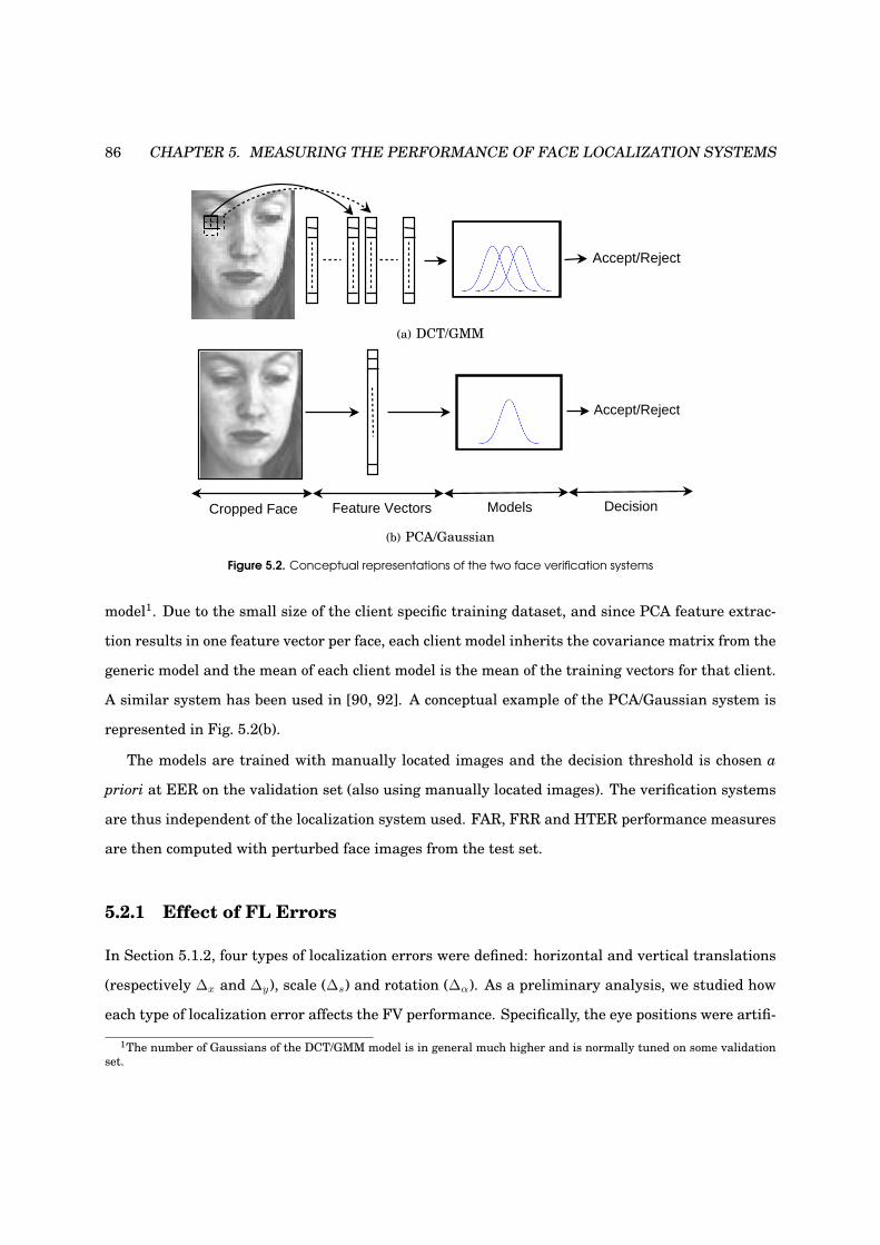
86 CHAPTER 5. MEASURING THE PERFORMANCE OF FACE LOCALIZATION SYSTEMS
Accept/Reject
(a) DCT/GMM
Feature VectorsCropped Face
Accept/Reject
Models Decision
(b) PCA/Gaussian
Figure 5.2. Conceptual representations of the two face verification systems
model1. Due to the small size of the client specific training dataset, and since PCA feature extrac-
tion results in one feature vector per face, each client model inherits the covariance matrix from the
generic model and the mean of each client model is the mean of the training vectors for that client.
A similar system has been used in [90, 92]. A conceptual example of the PCA/Gaussian system is
represented in Fig. 5.2(b).
The models are trained with manually located images and the decision threshold is chosen a
priori at EER on the validation set (also using manually located images). The verification systems
are thus independent of the localization system used. FAR, FRR and HTER performance measures
are then computed with perturbed face images from the test set.
5.2.1 Effect of FL Errors
In Section 5.1.2, four types of localization errors were defined: horizontal and vertical translations
(respectively ∆x and ∆y), scale (∆s) and rotation (∆α). As a preliminary analysis, we studied how
each type of localization error affects the FV performance. Specifically, the eye positions were artifi-
1The number of Gaussians of the DCT/GMM model is in general much higher and is normally tuned on some validation
set.

5.2. ROBUSTNESS OF CURRENT MEASURES 87
cially perturbed in order to generate a configurable amount of translation (horizontal and vertical),
scale and rotation errors. Then experiments were performed for each type of errors independently;
i.e. when we generated one type of perturbation, the others were kept null. Fig. 5.3 shows the FV
performance as a function of the generated perturbations for the two FV systems. Several conclu-
sions can be drawn from these curves:
1. Regarding HTER curves, as expected, the FV performance is affected by localization errors.
The minimum of the HTER curves are always obtained at the ground-truth positions.
2. In the tested range, FRR is more sensitive to localization errors, the FAR is not significantly
affected. In other words, localization errors in a reasonable range do not induce additional
false acceptances. This was expected since, after all, a non face rarely becomes a face by
simple geometric transpositions.
3. HTER curves demonstrate that the two FL approaches are not affected in the same way.
Generally, the DCT/GMM system is more robust to perturbed images than the PCA/Gaussian
system; justification of this result is discussed further in [11]. Moreover, we remark that the
two systems are not sensitive to the same type of errors; while DCT/GMM is affected by scale
and rotation errors and very robust to translation errors, the PCA/Gaussian system is very
sensitive to all types of errors, including translation.
5.2.2 Indetermination of deye
In Section 5.1, we discussed the important problem of a universal measure to evaluate face local-
ization performance, in order to get fair and clean system comparisons. We also introduced the
currently unique existing measure, proposed by Jesorsky et al. [39], based on the true and the de-
tected eye positions (5.1). We also underlined that this measure does not differentiate errors in
translation, scale or rotation.
For the specific task verification, prior empirical evidence showed that the performance is closely
related to the accuracy of the face localization system. In Section 5.2.1, we went further by ex-
plaining that this performance is closely related to the type of error introduced by the localization
system and that this dependency varies from one verification system to another (eg. DCT/GMM vs
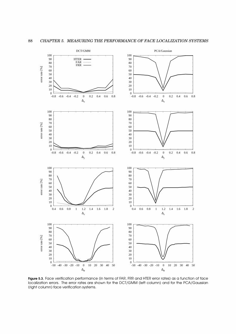
88 CHAPTER 5. MEASURING THE PERFORMANCE OF FACE LOCALIZATION SYSTEMS
100 90 80 70 60 50 40 30 20 10 0
-0.8 -0.6 -0.4 -0.2 0 0.2 0.4 0.6 0.8
erro
r ra
te [
%]
∆x
DCT/GMM
HTERFARFRR
100 90 80 70 60 50 40 30 20 10 0
-0.8 -0.6 -0.4 -0.2 0 0.2 0.4 0.6 0.8
erro
r ra
te [
%]
∆y
100 90 80 70 60 50 40 30 20 10 0
0.4 0.6 0.8 1 1.2 1.4 1.6 1.8 2
erro
r ra
te [
%]
∆s
100 90 80 70 60 50 40 30 20 10
0-50 -40 -30 -20 -10 0 10 20 30 40 50
erro
r ra
te [
%]
∆α
100 90 80 70 60 50 40 30 20 10
0-0.8 -0.6 -0.4 -0.2 0 0.2 0.4 0.6 0.8
∆x
PCA/Gaussian
100 90 80 70 60 50 40 30 20 10
0-0.8 -0.6 -0.4 -0.2 0 0.2 0.4 0.6 0.8
∆y
100 90 80 70 60 50 40 30 20 10
0 0.4 0.6 0.8 1 1.2 1.4 1.6 1.8 2
∆s
100 90 80 70 60 50 40 30 20 10
0-50 -40 -30 -20 -10 0 10 20 30 40 50
∆α
Figure 5.3. Face verification performance (in terms of FAR, FRR and HTER error rates) as a function of facelocalization errors. The error rates are shown for the DCT/GMM (left column) and for the PCA/Gaussian(right column) face verification systems.

5.2. ROBUSTNESS OF CURRENT MEASURES 89
PCA/Gaussian). We then argued that a universal criterion like deye is not adapted to the final task
of face verification and that we thus need to search for an application-dependent measure.
To illustrate this more clearly, let us look again at the deye measure and show why it is not
adapted to the FV task. In order to understand the limitations of this measure, we analyzed each
type of localization error independently, as done in Section 5.2.1.
Table 5.1. For the specific case of deye = 0.2, the first column contains the corresponding ∆ values and the third columncontains the resulting HTER
delta error deye HTER
∆x = −0.2 0.2 5.27
∆x = 0.2 0.2 5.43
∆y = −0.2 0.2 4.14
∆y = 0.2 0.2 3.27
∆s = 0.6 0.2 31.75
∆s = 1.4 0.2 24.65
∆α = 23 0.2 32.35
∆α = −23 0.2 31.24
We first arbitrarily selected a value of deye = 0.2, which commonly means that the detected
pattern is a face (since it is lower than 0.25). We then selected all kinds of delta errors which would
yield deye = 0.2. Details of how to obtain these corresponding delta errors are given in Appendix.
Fig. 5.4 shows examples of localizations obtained for each of these delta errors. The corresponding
∆ values are reported in the first column of Table 5.1. The last column shows the resulting face
verification performance, in terms of HTER, using the DCT/GMM face verification system. This
experiment basically shows the following:
1. There is a significant variation in HTER for the same value of deye.
2. The DCT/GMM system is more robust to errors in translation than to errors in scale or rota-
tion (for the same deye = 0.2).
Note that in practice, a face detector does not fail only on one type of error. However, this
experiment clearly shows that a face localization performance measure such as deye is not adapted
if we want to take into account the performance of the whole system.
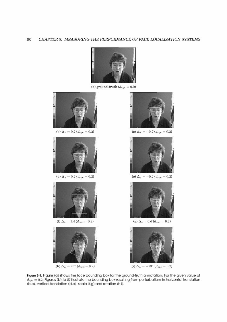
90 CHAPTER 5. MEASURING THE PERFORMANCE OF FACE LOCALIZATION SYSTEMS
(a) ground-truth (deye = 0.0)
(b) ∆x = 0.2 (deye = 0.2)
(d) ∆y = 0.2 (deye = 0.2)
(f) ∆s = 1.4 (deye = 0.2)
(h) ∆α = 23 (deye = 0.2)
(c) ∆x = −0.2 (deye = 0.2)
(e) ∆y = −0.2 (deye = 0.2)
(g) ∆s = 0.6 (deye = 0.2)
(i) ∆α = −23 (deye = 0.2)
Figure 5.4. Figure (a) shows the face bounding box for the ground-truth annotation. For the given value ofdeye = 0.2, Figures (b) to (i) illustrate the bounding box resulting from perturbations in horizontal translation(b,c), vertical translation (d,e), scale (f,g) and rotation (h,i).
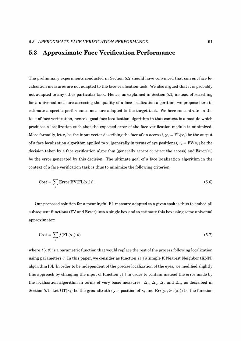
5.3. APPROXIMATE FACE VERIFICATION PERFORMANCE 91
5.3 Approximate Face Verification Performance
The preliminary experiments conducted in Section 5.2 should have convinced that current face lo-
calization measures are not adapted to the face verification task. We also argued that it is probably
not adapted to any other particular task. Hence, as explained in Section 5.1, instead of searching
for a universal measure assessing the quality of a face localization algorithm, we propose here to
estimate a specific performance measure adapted to the target task. We here concentrate on the
task of face verification, hence a good face localization algorithm in that context is a module which
produces a localization such that the expected error of the face verification module is minimized.
More formally, let xi be the input vector describing the face of an access i, yi = FL(xi) be the output
of a face localization algorithm applied to xi (generally in terms of eye positions), zi = FV(yi) be the
decision taken by a face verification algorithm (generally accept or reject the access) and Error(zi)
be the error generated by this decision. The ultimate goal of a face localization algorithm in the
context of a face verification task is thus to minimize the following criterion:
Cost =∑
i
Error(FV(FL(xi))) . (5.6)
Our proposed solution for a meaningful FL measure adapted to a given task is thus to embed all
subsequent functions (FV and Error) into a single box and to estimate this box using some universal
approximator:
Cost =∑
i
f(FL(xi); θ) (5.7)
where f(·; θ) is a parametric function that would replace the rest of the process following localization
using parameters θ. In this paper, we consider as function f(·) a simple K Nearest Neighbor (KNN)
algorithm [8]. In order to be independent of the precise localization of the eyes, we modified slightly
this approach by changing the input of function f(·) in order to contain instead the error made by
the localization algorithm in terms of very basic measures: ∆x, ∆y, ∆s and ∆α, as described in
Section 5.1. Let GT(xi) be the groundtruth eyes position of xi and Err(yi, GT(xi)) be the function

92 CHAPTER 5. MEASURING THE PERFORMANCE OF FACE LOCALIZATION SYSTEMS
that produces the face localization error vector; we thus have:
Cost =∑
i
f(Err(FL(xi), GT(xi)); θ) . (5.8)
To train such a function f(·), we used the following methodology. First, in order to cover the space
of localization errors, we create artificial examples based on all available training accesses. The
training examples of f(·) are thus uniformly generated by adding small perturbations (localization
errors) bounded by a reasonable range. For each generated example, a verification is performed
and a corresponding target value of 1 (respectively 0) is assigned when a verification error appears
(respectively does not appear).
5.4 Experiments and Results
This Section is devoted to verifying experimentally if our proposed method to measure the perfor-
mance of localization algorithms in the context of a face verification task improves with respect to
other known measures.
5.4.1 Training Data
The XM2VTS database was used to generate examples to estimate our function f(·), which should
yield the expected verification error given a localization error. For each of the 1000 available client
images2, 50 localization errors were randomly generated following a uniform distribution in a pre-
defined interval [−1, 1] for ∆x and ∆y, [0.5, 1.5] for ∆s and [−20, 20] for ∆α. The training set thus
contains 50000 examples. A verification is performed for each example, which will be assigned a
target value of 1 (respectively 0) when the verification algorithm accepts the client (respectively
rejects him). Furthermore, a separate validation set of 50000 examples was created using the same
procedure (with the same set of clients, but a different random seed).The hyper-parameter K of the
KNN model, which controls the capacity [104] of f(·), was then chosen as the one which minimized
the out-of-sample error on the validation set.
2The preliminary analysis of Section 5.2.1 showed that FAR is not significantly affected by localization errors, so we did
not use any impostor access for this step.

5.4. EXPERIMENTS AND RESULTS 93
5.4.2 Face Localization Performance Measure
Given the set of errors ∆ = ∆x,∆y,∆s,∆α generated by the FL algorithm on an image n we
define the error of the KNN localization algorithm as:
εKNN(∆n) =1
K
∑
k∈KNN(∆n)
Ck (5.9)
where KNN(∆n) is the set of the K nearest training examples of ∆n and Ck is the error made on
example k defined as:
Ck =
0 if Accepted Client
1 if Rejected Client .(5.10)
We then estimate the performance of the FL system on a set of N images using:
EKNN =1
N
N∑
n=1
εKNN(∆n) . (5.11)
Similarly, we measure the error made by the deye measure as follows:
εeye(n) =
0 if Accepted Client and deye(n) < 0.25
1 if otherwise(5.12)
and
Eeye =1
N
N∑
n=1
εeye(n) . (5.13)
5.4.3 KNN Function Evaluation
In order to verify that the obtained KNN function is robust to the choice of the training dataset,
we chose to evaluate it on another dataset, namely BANCA English (Section 4.3). In order to ex-
tract the faces from the access images, we use a modified version of the FDLBP face detection
system described in Section 2.4.5. This system involves some scanning parameters typically cho-
sen empirically, such as horizontal and vertical steps and scale factor. When minimizing these
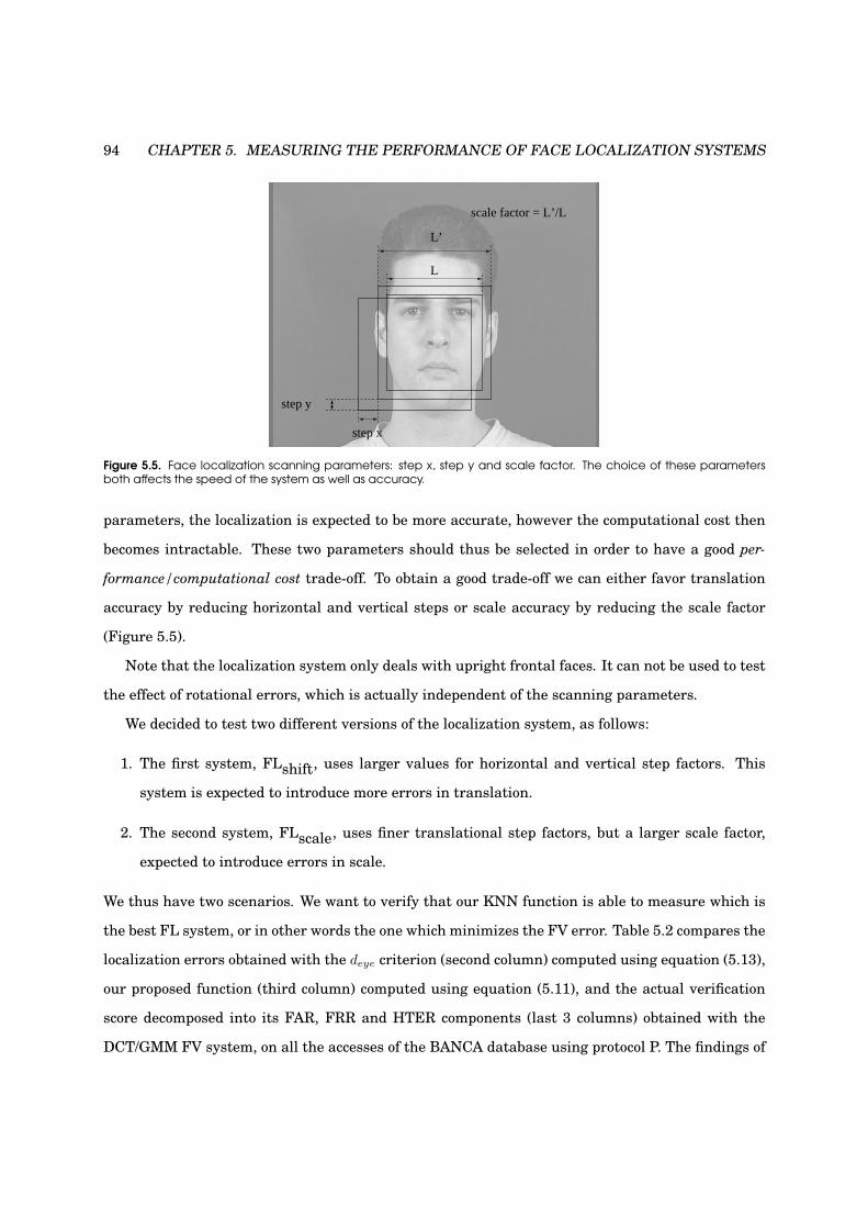
94 CHAPTER 5. MEASURING THE PERFORMANCE OF FACE LOCALIZATION SYSTEMS
L’
L
scale factor = L’/L
step x
step y
Figure 5.5. Face localization scanning parameters: step x, step y and scale factor. The choice of these parametersboth affects the speed of the system as well as accuracy.
parameters, the localization is expected to be more accurate, however the computational cost then
becomes intractable. These two parameters should thus be selected in order to have a good per-
formance/computational cost trade-off. To obtain a good trade-off we can either favor translation
accuracy by reducing horizontal and vertical steps or scale accuracy by reducing the scale factor
(Figure 5.5).
Note that the localization system only deals with upright frontal faces. It can not be used to test
the effect of rotational errors, which is actually independent of the scanning parameters.
We decided to test two different versions of the localization system, as follows:
1. The first system, FLshift, uses larger values for horizontal and vertical step factors. This
system is expected to introduce more errors in translation.
2. The second system, FLscale, uses finer translational step factors, but a larger scale factor,
expected to introduce errors in scale.
We thus have two scenarios. We want to verify that our KNN function is able to measure which is
the best FL system, or in other words the one which minimizes the FV error. Table 5.2 compares the
localization errors obtained with the deye criterion (second column) computed using equation (5.13),
our proposed function (third column) computed using equation (5.11), and the actual verification
score decomposed into its FAR, FRR and HTER components (last 3 columns) obtained with the
DCT/GMM FV system, on all the accesses of the BANCA database using protocol P. The findings of

5.4. EXPERIMENTS AND RESULTS 95
this experiment can be summarized as follows:
Table 5.2. Comparison of two FL performance measures for two face localization systems as well as for a perfectlocalization (ground-truth). The last 3 columns contains the face verification score in terms of FAR, FRR and HTER for theDCT/GMM system.
FL Systems Measures Verification
Eeye EKNN FAR [%] FRR [%] HTER [%]
ground-truth 0.00 0.05 15.1 23.9 19.5
FLshift 0.10 0.12 11.7 30.3 21.0
FLscale 0.04 0.15 14.7 33.8 24.3
1. As expected, the best verification score (HTER = 19.5) is obtained with perfect localization
(first conclusion of Section 5.2.1). Then follows the FLshift system, which yields an HTER of
21.0 and finally the FLscale system with an HTER of 24.3. This ordering was also expected,
following the third conclusion of Section 5.2.1.
2. Our proposed function correctly identifies the best localization system (FLshift, the system
which minimizes the face verification error), while the deye-based measure fails to order the
two modules. This can be mainly explained because the deye measure does not differentiate
errors in translation, shift or rotation, while the DCT/GMM FV system is more affected by a
certain type of error (third conclusion of Section 5.2.1).
3. The KNN almost perfectly predicts the FRR delta between the localization systems and the
groundtruth (0.12 − 0.05 ' (30.3 − 23.9)/100 and 0.15 − 0.12 ' (33.8 − 30.3)/100). Remember
that only client accesses were used to train the KNN function (Section 5.4.1).
4. We remark that the FAR corresponding to the FLshift system (11.7) and the FLscale system
(14.7) are lower than the FAR with perfect localization (15.1). This is because of impostor
accesses, a bad face localization only pushes the system to reject more accesses (including
impostors accesses), yielding a lower FAR.
Furthermore, the proposed KNN measure only takes 20 ms on a PIV 2.8 Ghz to evaluate an im-
age access, while it would take 350 ms for the DCT/GMM system (preprocessing, feature extraction
and classification).

96 CHAPTER 5. MEASURING THE PERFORMANCE OF FACE LOCALIZATION SYSTEMS
5.5 Conclusion
In this Chapter, we have proposed a novel methodology to compare face localization algorithms in
the context of the particular application of face verification. Note that the same methodology could
have been applied to any other task that builds on localization, such as face tracking. We have first
shown that current measures used in face localization are not accurate. We have thus proposed a
method to estimate the verification errors induced specifically by the use of a particular face local-
ization algorithm. This measure can then be used to compare more precisely several localization
algorithms. We tested our proposed measure using the BANCA database on a face verification task,
comparing two different face localization algorithms. Results show that our measure does indeed
capture more precisely the differences between localization algorithms (when applied to verifica-
tion tasks), which can be useful to select an appropriate localization algorithm. Furthermore, our
function is robust to the training dataset (training on XM2VTS and test on BANCA) and compared
to the DCT/GMM face verification system, the KNN performs more than 15 times faster (no prepro-
cessing and feature extraction steps). Finally, in order to compare FL modules, we do not need to
run face verification on the entire database, but we only use our function on a subset of face images.
In fact, one can view the process of training a localization system as a selection procedure where
one simply selects the best localization algorithm according to a given criterion. In that respect, an
interesting future work could concentrate on the use of such a measure to effectively train a face
localization system for the specific task of face verification.

Chapter 6
Conclusion
In this thesis, we presented a fully automatic face verification system which works in real-time
and which is robust to local illumination changes. The system is composed of two modules: face
detection and face verification. For both modules, we proposed a face representation based on Local
Binary Pattern (LBP) features. In this work, we considered face detection and verification as a
unified task. We argued that the measure to evaluate the detection step should include the final
task (here face verification) and that the verification step should be robust to the errors of the
detection module.
6.1 Face Detection
Most of the research in face detection has focused on the extension of the boosting based framework
of Viola and Jones [105]. These approaches generally suffer from a long training procedure and a
difficult optimal cascade design. In Chapter 2, we showed the advantages of LBP features compared
to traditional Haar-like features. Due to the higher discriminative power of the LBP, much fewer
features are needed for equivalent performances, leading to a much shorter training of the system
(hours instead of days) and to a simpler cascade design (3 cascade stages instead of more than 30).
Furthermore, we demonstrated on difficult lighting benchmarks that LBP features are more robust
to local illumination changes, as well as to partial occlusion of the face.
The fundamental issue of performance evaluation has also been discussed. We pointed out the
97
98 CHAPTER 6. CONCLUSION
necessity of a standard face criterion to determine what is a correctly detected face when reporting
error rates. However, this criterion is not enough to allow fair comparisons. Indeed, we empirically
demonstrated that the performance of a face detection system is affected by a wide range of factors
such as the training set, the image scanning parameters or the process of merging the overlapped
detections. Furthermore, in real-life applications, not only the accuracy but also the speed of the
face detection may be crucial.
In Chapter 3, we extended our frontal face detection system to deal with faces rotated in-plane
and out-of-plane. Our multiview system, based on an improved pyramid architecture, handles 16
different head poses but is only twice slower than the frontal face detector. We showed that the
multiview face detector achieves high detection performances but also that it produces many false
acceptances. We pointed out two possible future directions to cope with this limitation: 1) for
each pose, a post-processing classifier based on complementary discriminant features, 2) a more
sophisticated detection merging strategy.
Frontal face detection is now mature enough to be used in many practical applications, while
performances are not comparable with those obtained by humans. Face detection in a controlled
indoor environment has almost been solved, whereas it is still challenging to detect faces in out-
door unconstrained conditions (difficult lighting, cluttered background). However, one of the main
challenges in face detection is to deal with head pose variations, because face appearance variabil-
ity, due to lighting or facial expression is even larger for profile views than for frontal view. In
conclusion, more research is still needed in order to achieve robust multiview face detection.
6.2 Face Verification
In Chapter 4, we proposed a novel generative approach for face verification, based on a LBP de-
scription of the face. A generic face model was considered as a collection of LBP-histograms. A
client-specific model was then obtained by an adaptation technique from this generic model under
a probabilistic framework. We empirically showed that our proposed approach performs better than
state-of-the-art LBP-based face recognition techniques and is much faster than other state-of-the-
art face verification techniques that perform similarly than the proposed approach, for both manual
and automatic face localization. We also pointed out that our method, based on a holistic represen-
6.3. COMBINED FACE DETECTION AND VERIFICATION 99
tation of the face (concatenated LBP histograms), is very sensitive to small face localization errors
(due to the face detector) and to misalignment of facial features, such as the mouth or the eyes, with
respect to the face model (due to facial expressions). The next step would be to relax the constraints
on the location of the blocks and consider a more elastic grid of blocks (local representation). One
promising direction we are investigating is to look at the close neighborhood of each block and select
the region with the highest likelihood.
6.3 Combined Face Detection and Verification
In Chapter 5, we discussed the problem of the evaluation of face detection algorithms. We argued
that detection errors may have different impacts depending on the final application for which the
detection system has been designed, and thus that the evaluation measure should consider the
final task. We proposed a novel methodology to compare face detection algorithms in the context of
the particular application of face verification. We started by analyzing how detection errors affect
the performance of two face verification systems. This empirical analysis demonstrated that the
different types of detection errors, for instance errors in scale or rotation, do not induce the same
verification error, even if current detection performance measure would have rated them similarly.
We thus proposed a new measure which embeds the final application (here face verification) into
the performance measuring process. The proposed measure estimates directly the verification error
given the errors made by the detection system. We empirically showed that this measure can
be useful to efficiently select an appropriate face detection system. It is much faster to use our
measure on a subset of images than to run the face verification on entire databases. A future work
could concentrate on directly integrating such a function in the training process of a face detection
algorithm for the specific task of face verification.

100 CHAPTER 6. CONCLUSION

Acronyms
AFV Automatic Face Verification
ASM Active Shape Model
CART Classification And Regression Tree
CGM Constrained Generative Model
DCT Discrete Cosine Transform
DET Detection Error Trade-off
DR Detection Rate
EER Equal Error Rate
EPC Expected Performance Curve
FA False Acceptance
nFA number of False Acceptances
FAR False Acceptance Rate
FD Face Detection
FL Face Localization
FR False Rejection
FROC Free Receiver Operating Characteristic
FRR False Rejection Rate
FV Face Verification
GMM Gaussian Mixture Model
KNN K Nearest Neighbours
HCI Human Computer Interaction
HMM Hidden Markov Model
HTER Half Total Error Rate
LBP Local Binary Pattern
LDA Linear Discriminant Analysis
LP Lausanne Protocol
MAP Maximum A Posteriori
MLP Multi-Layer Perceptron
NC Normalized Correlation
PCA Principal Component Analysis
ROC Receiver Operating Characteristic
SNoW Sparse Network of Winnow
SVM Support Vector Machine
WER World Error Rate
101

102 CHAPTER 6. CONCLUSION

Appendix A
Face Localization using Active
Shape Models and LBP
This appendix addresses the problem of locating facial features in images of frontal faces taken un-
der different lighting conditions. The well-known Active Shape Model method proposed by Cootes
et al. is extended to improve its robustness to illumination changes. For that purpose, we introduce
the use of Local Binary Patterns (LBP). Experiments performed on the standard and darkened
image sets of the XM2VTS database demonstrate that our LBP-ASM approach gives superior per-
formance compared to the state-of-the-art ASM. It achieves more accurate results and fails less
frequently. Details can be found in our report [59].
A.1 Active Shape Models
Active Shape Model (ASM) is a popular statistical tool for locating examples of known objects in
images. It was first introduced by Cootes et al. [13] in 1995 and has been developed and improved
for many years. ASM is a model-based method which makes use of a prior model of what is expected
in the image. Basically, the Active Shape Model is composed of a deformable shape model and
a set of local appearance models. The shape model describes the typical variations of an object
exhibited in a set of manually annotated images and the local appearance models give a statistical
representation of the gray-level structures around each model point. Given a sufficiently accurate
103
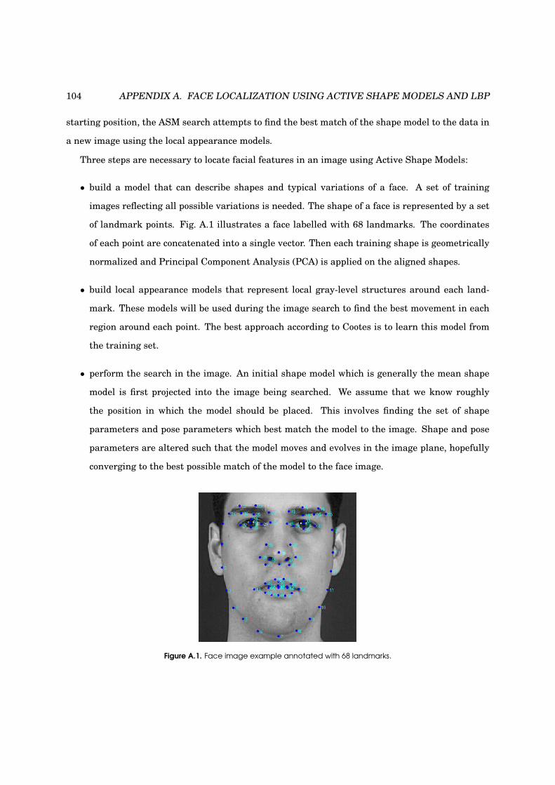
104 APPENDIX A. FACE LOCALIZATION USING ACTIVE SHAPE MODELS AND LBP
starting position, the ASM search attempts to find the best match of the shape model to the data in
a new image using the local appearance models.
Three steps are necessary to locate facial features in an image using Active Shape Models:
• build a model that can describe shapes and typical variations of a face. A set of training
images reflecting all possible variations is needed. The shape of a face is represented by a set
of landmark points. Fig. A.1 illustrates a face labelled with 68 landmarks. The coordinates
of each point are concatenated into a single vector. Then each training shape is geometrically
normalized and Principal Component Analysis (PCA) is applied on the aligned shapes.
• build local appearance models that represent local gray-level structures around each land-
mark. These models will be used during the image search to find the best movement in each
region around each point. The best approach according to Cootes is to learn this model from
the training set.
• perform the search in the image. An initial shape model which is generally the mean shape
model is first projected into the image being searched. We assume that we know roughly
the position in which the model should be placed. This involves finding the set of shape
parameters and pose parameters which best match the model to the image. Shape and pose
parameters are altered such that the model moves and evolves in the image plane, hopefully
converging to the best possible match of the model to the face image.
Figure A.1. Face image example annotated with 68 landmarks.
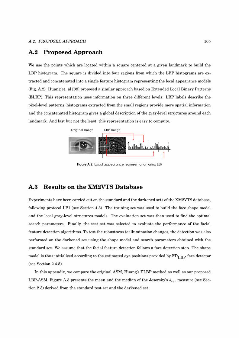
A.2. PROPOSED APPROACH 105
A.2 Proposed Approach
We use the points which are located within a square centered at a given landmark to build the
LBP histogram. The square is divided into four regions from which the LBP histograms are ex-
tracted and concatenated into a single feature histogram representing the local appearance models
(Fig. A.2). Huang et. al [38] proposed a similar approach based on Extended Local Binary Patterns
(ELBP). This representation uses information on three different levels: LBP labels describe the
pixel-level patterns, histograms extracted from the small regions provide more spatial information
and the concatenated histogram gives a global description of the gray-level structures around each
landmark. And last but not the least, this representation is easy to compute.
Figure A.2. Local appearance representation using LBP.
A.3 Results on the XM2VTS Database
Experiments have been carried out on the standard and the darkened sets of the XM2VTS database,
following protocol LP1 (see Section 4.3). The training set was used to build the face shape model
and the local gray-level structures models. The evaluation set was then used to find the optimal
search parameters. Finally, the test set was selected to evaluate the performance of the facial
feature detection algorithms. To test the robustness to illumination changes, the detection was also
performed on the darkened set using the shape model and search parameters obtained with the
standard set. We assume that the facial feature detection follows a face detection step. The shape
model is thus initialized according to the estimated eye positions provided by FDLBP face detector
(see Section 2.4.5).
In this appendix, we compare the original ASM, Huang’s ELBP method as well as our proposed
LBP-ASM. Figure A.3 presents the mean and the median of the Jesorsky’s deye measure (see Sec-
tion 2.3) derived from the standard test set and the darkened set.
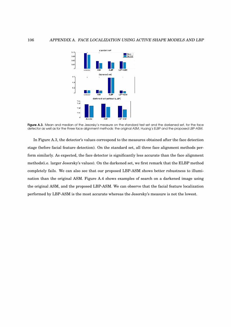
106 APPENDIX A. FACE LOCALIZATION USING ACTIVE SHAPE MODELS AND LBP
Figure A.3. Mean and median of the Jesorsky’s measure on the standard test set and the darkened set, for the facedetector as well as for the three face alignment methods: the original ASM, Huang’s ELBP and the proposed LBP-ASM.
In Figure A.3, the detector’s values correspond to the measures obtained after the face detection
stage (before facial feature detection). On the standard set, all three face alignment methods per-
form similarly. As expected, the face detector is significantly less accurate than the face alignment
methods(i.e. larger Jesorsky’s values). On the darkened set, we first remark that the ELBP method
completely fails. We can also see that our proposed LBP-ASM shows better robustness to illumi-
nation than the original ASM. Figure A.4 shows examples of search on a darkened image using
the original ASM, and the proposed LBP-ASM. We can observe that the facial feature localization
performed by LBP-ASM is the most accurate whereas the Jesorsky’s measure is not the lowest.
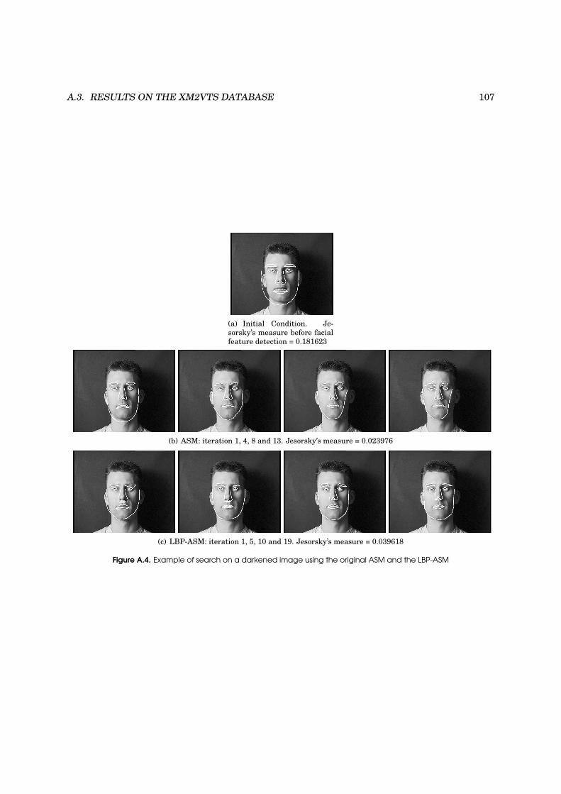
A.3. RESULTS ON THE XM2VTS DATABASE 107
(a) Initial Condition. Je-
sorsky’s measure before facial
feature detection = 0.181623
(b) ASM: iteration 1, 4, 8 and 13. Jesorsky’s measure = 0.023976
(c) LBP-ASM: iteration 1, 5, 10 and 19. Jesorsky’s measure = 0.039618
Figure A.4. Example of search on a darkened image using the original ASM and the LBP-ASM

108 APPENDIX A. FACE LOCALIZATION USING ACTIVE SHAPE MODELS AND LBP
Appendix B
Hand Posture Classification and
Recognition using LBP
Developing new techniques for human-computer interaction is very challenging. Vision-based tech-
niques have the advantage of being unobtrusive and hands are a natural device that can be used
for more intuitive interfaces. But in order to use hands for interaction, it is necessary to be able
to recognize them in images. In [43], we propose to apply the approach described in Section 2.2 for
face detection to the tasks of hand posture classification and recognition. This approach is based on
the boosting of Local Binary Patterns (LBP) features. A two-class model is trained for each hand
posture. The positive training set is composed of samples of the hand posture, while the negative
set is composed of background images as well as images of the other postures. Each posture model
is a one-stage classifier composed of 500 weak classifiers, trained with 2500 boosting iterations.
B.1 Database and Protocols
Results are reported on the Jochen Triesch database 1. It consists of 10 hand signs performed by
24 different people against 3 types of backgrounds (720 images): uniform light, uniform dark and
complex (Fig. B.1) The database is partionned into three subsets: train, validation and test. For
Protocol 1, training and validation sets are composed only of images in uniform background while
1http://www-prima.inrialpes.fr/FGnet/data/09-Pets2002/data/POSTURE/
109

110 APPENDIX B. HAND POSTURE CLASSIFICATION AND RECOGNITION USING LBP
(a) 10 hand postures (b) 3 types of backgrounds
Figure B.1. The Jochen Triesch hand posture database.
for Protocol 2, both sets include the images in complex background.
Following the method presented in Section 2.4.1 for faces, hand postures images are first cropped
according to manual annotation and then subsampled to the size of 30 × 30 pixels, followed by his-
togram equalisation. Training and validation sets have been extended by slightly shifting, scaling
and rotating the original images. 30 virtual samples have been created for each original image.
B.2 Hand Posture Classification
First, we would like to verify that our model is able to perform correct classification for each hand
posture. Classification rates are reported in Table B.1.
1. Background: Most hand postures are correctly classified. As expected, classification rate
with uniform background (99.2%) provides better results than with complex background (89.8%).
2. Posture: With uniform background, all postures are well classified. With complex back-
ground, better performance is obtained for Protocol 2 (matched conditions). With Protocol 1,
we remark that some postures (’C’, ’V’, ’Y’) are difficult to classify.
3. Protocol: For Protocol 2, almost all postures are well classified in both background conditions.
For Protocol 1 (no training data in complex background), the classification rate decreases for
all postures.

B.3. HAND POSTURE RECOGNITION 111
Table B.1. Classification rate (in %) on the test set
Uniform Background Complex Background
Protocol1 Protocol2 Protocol1 Protocol2
A 100 100 91.67 100
B 93.75 100 75 100
C 96.88 100 66.67 93.75
D 100 100 87.5 100
G 100 100 87.5 100
H 100 100 100 100
I 100 100 95.83 93.75
L 100 100 100 100
V 96.77 100 54.17 100
Y 96.88 100 62.5 87.5
average 98.4 100 82.1 97.5
B.3 Hand Posture Recognition
This section concerns the recognition task, i.e. given a unknown posture, we would like to identify
its posture class label. For that purpose, we chose a “one versus all” strategy. For a given posture
test image, we apply all posture models and consider the one with the highest score to label the test
image. Recognition rates are reported in Table B.2.
1. Background: Recognition rate is higher for the images against uniform than complex back-
ground. We notice that some postures are not sensitive to the background type such as ’A’ or
’B’, while other postures are strongly affected, such as ’G’, ’I’, ’L’, ’V’ or ’Y’. The common fea-
tures of these postures is a closed fist with one ore two thin pointing fingers, which are “sunk”
in the background and thus difficult to find out.
2. Posture: Some postures like ’A’ are easier to recognize, regardless of the background type.
On the other hand, the ’Y’ posture achieves the lowest recognition rate in both conditions. The
explanation may be found in the high variability of the hand posture shape. While the ’B’
posture will be performed in a similar manner by every gesturer, it will not be the case with
the ’Y’ posture.

112 APPENDIX B. HAND POSTURE CLASSIFICATION AND RECOGNITION USING LBP
Table B.2. Recognition rate (in %) on the test set
Uniform Background Complex Background
Protocol1 Protocol2 Protocol1 Protocol2
A 100 100 100 100
B 93.75 93.75 93.75 93.75
C 93.75 93.75 75 93.75
D 93.75 84.38 62.5 81.25
G 96.88 100 50 68.75
H 84.38 90.63 87.5 87.5
I 84.38 90.63 56.25 62.5
L 84.38 96.88 37.5 75
V 87.10 96.77 56.25 87.5
Y 81.25 81.25 25 62.5
average 89.97 92.79 64.38 81.25
3. Protocol: Like for classification, better performance is achieved with Protocol 2 (matched con-
ditions). However, the protocol does not affect each posture in the same way. While postures
’A’ or ’B’ are robust to the protocol, postures ’L’ or ’Y’ are dramatically affected.
Preliminary results are encouraging, although some postures (’G’, ’I’, ’Y’) are difficult to recog-
nize. The next step to a fully automatic hand posture recognition system would be the segmentation
of the hand which was done manually in this work.
Appendix C
Texture Representation for
Illumination Robust Face
Verification
One of the major problem in face verification systems is to deal with variations in illumination.
In a realistic scenario, it is very likely that the lighting conditions of the probe image does not
correspond to those of the gallery image, hence there is a need to handle such variations. In [32],
we present a new preprocessing algorithm based on Local Binary Patterns (LBP): a texture rep-
resentation is derived from the input face image before being forwarded to the classifier. The effi-
ciency of the proposed approach is empirically demonstrated using both an appearance-based (PCA-
LDA) and a feature-based (1D-HMM) face verification systems on BANCA and XM2VTS databases
(Section 4.3). Three illumination normalization techniques are compared: the standard histogram
equalization, the state-of-the-art Gross and Brajovic [27] method and the proposed LBP approach.
Details on these normalization techniques as well as on both face verification systems can be found
in the paper [43]. Tables C.1 and C.2 show comparative face verification results.
113
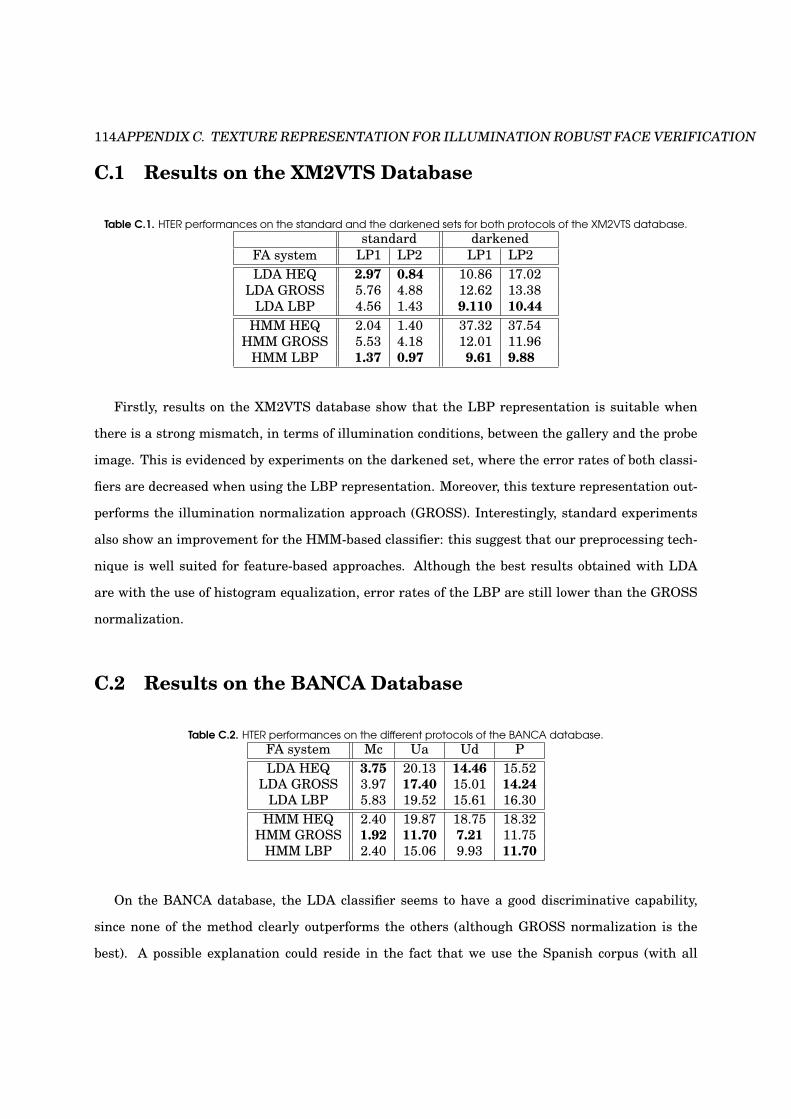
114APPENDIX C. TEXTURE REPRESENTATION FOR ILLUMINATION ROBUST FACE VERIFICATION
C.1 Results on the XM2VTS Database
Table C.1. HTER performances on the standard and the darkened sets for both protocols of the XM2VTS database.standard darkened
FA system LP1 LP2 LP1 LP2
LDA HEQ 2.97 0.84 10.86 17.02
LDA GROSS 5.76 4.88 12.62 13.38
LDA LBP 4.56 1.43 9.110 10.44
HMM HEQ 2.04 1.40 37.32 37.54
HMM GROSS 5.53 4.18 12.01 11.96
HMM LBP 1.37 0.97 9.61 9.88
Firstly, results on the XM2VTS database show that the LBP representation is suitable when
there is a strong mismatch, in terms of illumination conditions, between the gallery and the probe
image. This is evidenced by experiments on the darkened set, where the error rates of both classi-
fiers are decreased when using the LBP representation. Moreover, this texture representation out-
performs the illumination normalization approach (GROSS). Interestingly, standard experiments
also show an improvement for the HMM-based classifier: this suggest that our preprocessing tech-
nique is well suited for feature-based approaches. Although the best results obtained with LDA
are with the use of histogram equalization, error rates of the LBP are still lower than the GROSS
normalization.
C.2 Results on the BANCA Database
Table C.2. HTER performances on the different protocols of the BANCA database.FA system Mc Ua Ud P
LDA HEQ 3.75 20.13 14.46 15.52
LDA GROSS 3.97 17.40 15.01 14.24
LDA LBP 5.83 19.52 15.61 16.30
HMM HEQ 2.40 19.87 18.75 18.32
HMM GROSS 1.92 11.70 7.21 11.75
HMM LBP 2.40 15.06 9.93 11.70
On the BANCA database, the LDA classifier seems to have a good discriminative capability,
since none of the method clearly outperforms the others (although GROSS normalization is the
best). A possible explanation could reside in the fact that we use the Spanish corpus (with all

C.2. RESULTS ON THE BANCA DATABASE 115
scenarios) to train the LDA, hence it may capture by itself the changes in acquisition conditions.
Concerning the HMM-based classifier, GROSS normalization results are better for three of the four
investigated protocol, and reduces error rates by a significant amount compared to histogram equal-
ization. Results obtained with the LBP representation are comparable, although performances are
a bit worse.
To summarize, conducted experiments shows that the proposed preprocessing approach is suit-
able for face verification: results are comparable with, or even better than those obtained using
the state-of-the-art preprocessing algorithm proposed in [27]. Moreover, the LBP representation
is simpler, faster to compute and there is no need for hyper-parameter selection, hence avoiding
extensive experiments.

116APPENDIX C. TEXTURE REPRESENTATION FOR ILLUMINATION ROBUST FACE VERIFICATION
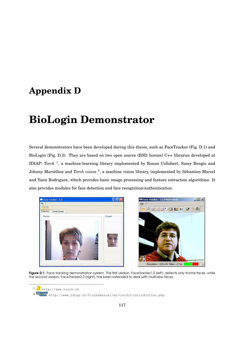
Appendix D
BioLogin Demonstrator
Several demonstrators have been developed during this thesis, such as FaceTracker (Fig. D.1) and
BioLogin (Fig. D.2). They are based on two open source (BSD license) C++ libraries developed at
IDIAP: Torch 1, a machine-learning library implemented by Ronan Collobert, Samy Bengio and
Johnny Mariéthoz and Torch vision 2, a machine vision library, implemented by Sébastien Marcel
and Yann Rodriguez, which provides basic image processing and feature extraction algorithms. It
also provides modules for face detection and face recognition/authentication.
Figure D.1. Face tracking demonstration system. The first version, FaceTracker1.0 (left), detects only frontal faces, whilethe second version, FaceTracker2.0 (right), has been extended to deal with multiview faces.
1 http://www.torch.ch
2 http://www.idiap.ch/$\sim$marcel/en/torch3/introduction.php
117

118 APPENDIX D. BIOLOGIN DEMONSTRATOR
Figure D.2. Bimodal Authentication system based on face, speech and fusion developed at IDIAP. The system providesa BioLogin application (left) to test a client, and a Manager application (right) to create a new account by enrollment.
In this appendix, we will only focus on BioLogin, a multimodal (face and speech) authentication
demonstration system that simulates the login of a user using its face and its voice. It runs both on
Linux and Windows and the Windows version is freely available for download at 3.
The system (Fig. D.2) includes two applications:
• BioLogin: login using the face and the voice (test a biometric template),
• User Manager: creates a new account and enables the user to enroll a biometric template.
First the user needs to create his/her account using the Manager application. The registration
consists in (1) filling a form and (2) recording a session of four audio/video shots. During each shot,
the system asks the user to pronounce his/her pass-phrase. The audio recording starts when a face
is detected and stops when the time is elapsed or when the user press <enter>. Face images are
automatically captured during the audio recording. At the end of the recording session, the user
can visualize/listen to the recordings. The user can decide to cancel the recording session and to
perform another one or to enroll his/her model from recordered data. The enrollment process takes
only few seconds. Finally, the user can launch the BioLogin application. This application presents
a list of registered persons. To perform an authentication test, the user simply needs to select a
person. Then the audio/video capture is immediately launched. As soon as the face is detected, the
3 http://www.idiap.ch/biologin

119
user has a few seconds to pronounce the pass-phrase. If the time is elapsed or if the user press
<enter> then the authentication is performed. The system displays either accepted in green if
the user is considered as a client or rejected in red if the user is considered as an impostor.
BioLogin has been internationally recognized as a finalist of the Swiss Technology Awards 2006
and presented at the CeBIT trade in Hannover.

120 APPENDIX D. BIOLOGIN DEMONSTRATOR

Bibliography
[1] T. Ahonen, A. Hadid, and M. Pietikäinen. Face recognition with local binary patterns. In
Proc. 8th European Conference on Computer Vision (ECCV), pages 469–481, Prague, Czech
Republic, 2004.
[2] S. Ba and J.-M. Odobez. A rao-blackwellized mixed state particle filter for head pose tracking
in meetings. In Proceedings of the ACM ICMI Workshop on Multimodal Multiparty Meeting
Processing (MMMP), pages 9–16, Trento, Italy, 2004.
[3] E. Bailly-Baillière, S. Bengio, F. Bimbot, M. Hamouz, J. Kittler, J. Mariéthoz, J. Matas,
K. Messer, V. Popovici, F. Porée, B. Ruiz, and J.-P. Thiran. The BANCA database and evalua-
tion protocol. In Proceedings of the 4th International Conference on Audio- and Video-Based
Biometric Person Authentication (AVBPA), pages 625–638, Guilford, UK, 2003.
[4] M. Bartlett, J. Movellan, and T. Sejnowski. Face recognition by independent component anal-
ysis. IEEE Transactions on Neural Networks, 13(6):1450–1464, 2002.
[5] S. Behnke. Face localization in the neural abstraction pyramid. In Proceedings of the 7th In-
ternational Conference on Knowledge-Based Intelligent Information and Engineering Systems
(KES), pages 139–145, Oxford, UK, 2003.
[6] P. Belhumeur, J.P. Hespanha, and D.J. Kriegman. Eigenfaces vs. Fisherfaces: Recognition
using class specific linear projection. In Proceedings of the Fourth European Conference on
Computer Vision, pages 45–58, Cambridge, United Kingdom, 1996.
[7] S. Bengio and J. Mariéthoz. The expected performance curve: a new assessment measure for
121

122 BIBLIOGRAPHY
person authentication. In Proceedings of Odyssey 2004: The Speaker and Language Recogni-
tion Workshop, pages 279–284, Toledo, Spain, 2004.
[8] C. Bishop. Neural Networks for Pattern Recognition. Oxford University Press, 1995.
[9] S. Brubaker, J. Wu, J. Sun, M. Mullin, and J. Rehg. On the design of cascades of boosted en-
sembles for face detection. Technical Report GIT-GVU-05-28, Georgia Institute of Technology,
2005.
[10] F. Cardinaux, C. Sanderson, and S. Bengio. Face verification using adapted generative mod-
els. In Proceedings of the 6th IEEE International Conference on Automatic Face and Gesture
Recognition (AFGR), pages 825–830, Seoul, Korea, 2004.
[11] F. Cardinaux, C. Sanderson, and S. Bengio. User authentication via adapted statistical mod-
els of face images. To appear in IEEE Transaction on Signal Processing, 2005.
[12] F. Cardinaux, C. Sanderson, and S. Marcel. Comparison of MLP and GMM classifiers for face
verification on XM2VTS. In Proceedings of the 4th International Conference on Audio- and
Video-Based Biometric Person Authentication (AVBPA), pages 911–920, Guilford, UK, 2003.
[13] T. Cootes, C. Taylor, D. Cooper, and J. Graham. Active Shape Models - their training and
applications. Computer Vision and Image Understanding, 61:38–59, 1995.
[14] T. Cootes, K. Walker, and C. Taylor. View-based active appearance models. In Proceedings of
the IEEE Conference on Automatic Face and Gesture Recognition, pages 227–232, 2000.
[15] D. Cristinacce. Automatic Detection of Facial Features in Grey Scale Images. PhD thesis,
University of Manchester, 2004.
[16] F Crow. Summed-area tables for texture mapping. In Proceedings of SIGGRAPH, Computer
Graphics, pages 207–212, 1984.
[17] L.G. Farkas. Anthropometry of the Head and Face. Raven Press, 1994.
[18] I.R. Fasel and J.R. Movellan. Meta analysis of neurally inspired face detection algorithms. In
Proceedings of the Eighth Joint Symposium on Neural Computation, 2001.

BIBLIOGRAPHY 123
[19] R. Féraud, O. Bernier, and D. Collobert. A constrained generative model applied to face
detection. In Proceedings of the Fourteenth National Conference on Artificial Intelligence,
1997.
[20] Y. Freund and R.E. Schapire. Experiments with a new boosting algorithm. In Proceedings of
the IEEE International Conference on Machine Learning (ICML), pages 148–156, Bari, Italy,
1996.
[21] J. Friedman, T. Hastie, and R. Tibshirani. Additive logistic regression: a statistical view of
boosting. The Annals of Statistics, 28(2):337–374, 2000.
[22] B. Fröba and A. Ernst. Face detection with the modified census transform. In Proceedings of
the 6th IEEE International Conference on Automatic Face and Gesture Recognition (AFGR),
pages 91–96, Seoul, Korea, 2004.
[23] B. Fröba and C. Küblbeck. Robust face detection at video frame rate based on edge orientation
features. In Proceedings of the 5th IEEE International Conference on Automatic Face and
Gesture Recognition (AFGR), pages 342–347, Washington, D.C., USA, 2002.
[24] C. Garcia and M. Delakis. Convolutional face finder: A neural architecture for fast and robust
face detection. IEEE Transactions on Pattern Analysis and Machine Intelligence, 26(11), 2004.
[25] J.L. Gauvain and C.-H. Lee. Maximum a posteriori estimation for multivariate gaussian
mixture observation of markov chains. In IEEE Transactions on Speech Audio Processing,
volume 2, pages 291–298, 1994.
[26] N. Gourier, D. Hall, and J. L. Crowley. Estimating face orientation from robust detection of
salient facial features. In Proceedings of Pointing 2004, ICPR, International Workshop on
Visual Observation of Deictic Gestures, Cambridge, UK, 2004.
[27] R. Gross and V. Brajovic. An image preprocessing algorithm for illumination invariant face
recognition. In Proceedings of the 4th International Conference on Audio- and Video-Based
Biometric Person Authentication (AVBPA), Guilford, UK, 2003.
[28] E. Grossman. Automatic design of cascaded classifiers. In Joint IAPR International Work-
shops SSPR/SPR, pages 983–991, Lisbon, Portugal, 2004.

124 BIBLIOGRAPHY
[29] A. Hadid, M. Pietikäinen, and T. Ahonen. A discriminative feature space for detecting and
recognizing faces. In Proceedings of the IEEE Conference on Computer Vision and Pattern
Recognition (CVPR), pages 797–804, Washignton D.C., USA, 2004.
[30] M. Hamouz, J. Kittler, J.-K. Kamarainen, P. Paalanen, and H. K Kälviäinen. Affine-invariant
face detection and localization using gmm-based feature detector and enhanced appearance
model. In Proceedings of the 6th IEEE International Conference on Automatic Face and Ges-
ture Recognition (AFGR), pages 67–72, Seoul, Korea, 2004.
[31] M. Heikkilä, M. Pietikäinen, and J. Heikkilä. A texture-based method for detecting moving
objects. In Proc. the 15th British Machine Vision Conference (BMVC), pages 187–196, London,
UK, 2004.
[32] G. Heusch, Y. Rodriguez, and S. Marcel. Local binary patterns as an image preprocessing for
face authentication. In Proceedings of the 7th IEEE Int. Conf. on Automatic Face and Gesture
Recognition (AFGR), pages 9–14, Southampton, UK, April 10-12 2006.
[33] E. Hjelmas and B.K. Low. Face detection: A survey. Computer Vision and Image Understand-
ing, 83:236–274, 2001.
[34] C. Huang, H. Ai, Y. Li, and S. Lao. Vector boosting for rotation invariant multi-view face
detection. In Proceedings of the IEEE Conference on Computer Vision (ICCV), pages 446–453,
Beijing, China, 2005.
[35] K.S. Huang and M.M. Trivedi. Robust real-time detection, tracking, and pose estimation of
face in video streams. In Proceedings of the International Conference on Pattern Recognition
(ICPR), pages 965–968, Cambridge, UK, 2004.
[36] R.-J. Huang. Detection Strategies for Face Recognition Using Learning and Evolution. PhD
thesis, George Mason University, Fairfax, Virginia, 1998.
[37] X. Huang, S. Z. Li, and Y. Wang. Jensen-shannon boosting learning for object recognition. In
Proc. IEEE Int. Conf. on Computer Vision and Pattern Recognition (CVPR), San Diego, USA,
2005.

BIBLIOGRAPHY 125
[38] X. Huang, S.Z. Li, and Y. Wang. Shape localization based on statistical method using extended
local binary pattern. In Proc. Third International Conference on Image and Graphics (ICIG),
pages 184–187, Hong Kong, China, 2004.
[39] O. Jesorsky, K. Kirchberg, and R. Frischholz. Robust face detection using the hausdorff dis-
tance. In Proceedings of the 3rd International Conference on Audio- and Video-Based Biomet-
ric Person Authentication (AVBPA), pages 90–95, Halmstad, Sweden, 2001.
[40] H. Jin, Q. Liu, H. Lu, and X. Tong. Face detection using improved LBP under bayesian
framework. In Proc. Third International Conference on Image and Graphics (ICIG), pages
306–309, Hong Kong, China, 2004.
[41] M Jones and P. Viola. Fast multi-view face detection. In IEEE Conference on Computer Vision
and Pattern Recognition, 2003.
[42] K. Jonsson, J. Matas, J. Kittler, and Y.P. Li. Learning support vectors for face verification
and recognition. In 4th International Conference on Automatic Face and Gesture Recognition,
pages 208–213, 2000.
[43] A. Just, Y. Rodriguez, and S. Marcel. Hand posture classification and recognition using the
modified census transform. In Proceedings of the 7th IEEE Int. Conf. on Automatic Face and
Gesture Recognition (AFGR), Southampton, UK, April 10-12 2006.
[44] T. Kanade. Picture processing by computer complex and recognition of human faces. PhD
thesis, University of Kyoto, 1973.
[45] D. Le and S. Satoh. Multi-stage approach to fast face detection. In Proc. the 16th British
Machine Vision Conference (BMVC), Oxford, UK, 2005.
[46] S.Z. Li and Z. Zhang. Floatboost learning and statistical face detection. IEEE Transactions
on Pattern Analysis and Machine Intelligence (PAMI), 26(9):1112–1123, 2004.
[47] Y. Li, S. Gong, J. Sherrah, and H. Liddell. Support vector machine based multi-view face
detection and recognition. Image and Vision Computing, 22:413–427, 2004.

126 BIBLIOGRAPHY
[48] Y. Li, J. Kittler, and J. Matas. On matching scores of LDA-based face verification. In T. Prid-
more and D. Elliman, editors, Proceedings of the British Machine Vision Conference. British
Machine Vision Association, 2000.
[49] R. Lienhart, A. Kuranov, and V. Pisarevsky. Empirical analysis of detection cascades of
boosted classifiers for rapid object detection. In Proceedings of the 25th DAGM-Symposium,
pages 297–304, Magdeburg, Germany, 2003.
[50] N. Littlestone. Learning quickly when irrelevant attributes abound: a new linear-threshold
algorithm. Machine Learning, 2:285–318, 1988.
[51] C. Liu and H. Shum. Kullback-leibler boosting. In Proceedings of the IEEE Conference on
Computer Vision and Pattern Recognition (CVPR), pages 407–411, Madison, USA, 2003.
[52] J. Lu, K. Plataniotis, and A. Venetsanopoulos. Face recognition using lda based algorithms.
IEEE Transactions on Neural Networks, 14(1), 2003.
[53] S. Lucey and T. Chen. A GMM parts based face representation for improved verification
through relevance adaptation. In Proc. IEEE Int. Conf. on Computer Vision and Pattern
Recognition (CVPR), Washington D.C., USA, 2004.
[54] H. Luo. Optimization design of cascaded classifiers. In Proc. IEEE Int. Conf. on Computer
Vision and Pattern Recognition (CVPR), pages 480–485, San Diego, USA, 2005.
[55] J. Lüttin and G. Maître. Evaluation protocol for the extended m2vts database (xm2vtsdb).
IDIAP Communication 98-05, IDIAP Research Institute, Martigny, Switzerland, 1998.
[56] Y Ma and X. Ding. Robust real-time face detection based on cost-sensitive adaboost method.
In Proceedings of the International Conference on Multimedia and Expo (ICME), pages 465–
468, Baltimore, USA, 2003.
[57] S. Marcel. A symmetric transformation for LDA-based face verification. In Proceedings of the
6th International Conference on Automatic Face and Gesture Recognition, 2004.
[58] S. Marcel and S. Bengio. Improving face verification using skin color information. In Proceed-
ings of the 16th International Conference on Pattern Recognition (ICPR), Québec, Canada,
2002.

BIBLIOGRAPHY 127
[59] S. Marcel, J. Keomany, and Y. Rodriguez. Robust-to-illumination face localisation using ac-
tive shape models and local binary patterns. IDIAP-RR 47, IDIAP, 2006. Submitted for
publication.
[60] S. Marcel, J. Mariéthoz, Y. Rodriguez, and F. Cardinaux. Bi-modal face and speech authenti-
cation: a biologin demonstration system. In 2nd Workshop on Multimodal User Authentica-
tion (MMUA), Toulouse, France, May 11-12 2006.
[61] A. Martin, G. Doddington, T. Kamm, M. Ordowski, and M. Przybocki. The DET curve in
assessment of detection task performance. In Proceedings of Eurospeech’97, pages 1895–
1898, Rhodes, Greece, 1997.
[62] A Martinez. Recognizing imprecisely localized, partially occluded, and expression variant
faces from a single sample per class. IEEE Transactions on Pattern Analysis and Machine
Intelligence, 24(6):748–763, 2002.
[63] A. Martinez and R. Benavente. The AR face database. Technical Report CVC24, Purdue
University, 1998.
[64] B. McCane and K. Novins. On training cascade face detectors. In Proceedings of Image and
Vision Computing New Zealand, pages 239–244, 2003.
[65] R. Meir and G. Rätsch. An introduction to Boosting and Leveraging. Springer, 2003.
[66] K. Messer, K. Kittler, J. Short, G. Heusch, F. Cardinaux, S. Marcel, Y. Rodriguez, and al.
Performance characterization of face recognition algorithms and their sensitivity to severe
illumination changes. In Proceedings of the International Conference on Biometrics (ICB),
pages 1–11, Hong Kong, January 5-7 2006.
[67] K. Messer, J. Matas, J. Kittler, J. Luettin, and G. Maitre. XM2VTSDB: The extended M2VTS
database. In Proceedings of the 2nd International Conference on Audio and Video-based Bio-
metric Person Authentication, 1999.
[68] T. Mita, Kaneko T., and O. Hori. Joint haar-like features for face detection. In Proceedings
of the 10th IEEE International Conference on Computer Vision (ICCV), pages 1619–1626,
Washington D.C., USA, 2005.

128 BIBLIOGRAPHY
[69] B. Moghaddam, T. Jebara, and A. Pentland. Bayesian face recognition. Pattern Recognition,
33:1771–1782, 2000.
[70] Y. Moses, Y. Adini, and S. Ullman. Face recognition: the problem of compensating for changes
in illumination direction. In Proc. 3rd European Conference on Computer Vision (ECCV),
pages 286–296, Stockholm, Sweden, 1994.
[71] A. Nefian and M. Hayes. Face recognition using an embedded HMM. In Proceedings of the
IEEE Conference on Audio and Video-based Biometric Person Authentication (AVBPA), pages
19–24, 1999.
[72] A. Nefian, M. Hayes, and III. Face detection and recognition using hidden markov models.
In Proceedings of the IEEE International Conference on Image Processing, volume 1, pages
141–145, 1998.
[73] T. Ojala, M. Pietikäinen, and D. Harwood. A comparative study of texture measures with
classification based on feature distributions. Pattern Recognition, 29, 1996.
[74] T. Ojala, M. Pietikäinen, and T. Mäenpää. Multiresolution gray-scale and rotation invariant
texture classification with local binary patterns. IEEE Transactions on Pattern Analysis and
Machine intelligence, 24:971–987, 2002.
[75] E. Osuna, Freund R., and F. Girosi. Training svm: An application to face detection. In
Proceedings of the IEEE Conference on Computer Vision and Pattern Recognition, pages 130–
136, 1997.
[76] C. Papageorgiou, M. Oren, and T. Poggio. A general framework for object detection. In Pro-
ceedings of the IEEE International Conference on Computer Vision, pages 555–562, 1998.
[77] V. Pavlovic and A. Garg. Efficient detection of objects and attributes using boosting. In
Proceedings of the IEEE Conference on Computer Vision and Pattern Recognition, 2001.
[78] P. Phillips, H. Moon, S. Rizvi, and P. Rauss. The feret evaluation methodology for face recog-
nition algorithms. IEEE Transactions on Pattern Analysis and Machine Intelligence, 22(10),
2000.

BIBLIOGRAPHY 129
[79] V. Popovici and J.-P. Thiran. Face detection using svm trained in eigenfaces space. In Pro-
ceedings of the 4th International Conference on Audio- and Video-Based Biometric Person
Authentication, pages 925–928, 2003.
[80] V. Popovici, J.-P. Thiran, Y. Rodriguez, and S. Marcel. On performance evaluation of face
detection and localization algorithms. In Proceedings of the 17th International Conference on
Pattern Recognition (ICPR), pages 313–317, Cambridge, UK, August 23-26 2004.
[81] Douglas A. Reynolds, Thomas F. Quatieri, and Robert B. Dunn. Speaker verification using
adapted gaussian mixture models. Digital Signal Processing, 10(1-3):19–41, 2000.
[82] Y. Rodriguez, F. Cardinaux, S. Bengio, and J. Mariéthoz. Estimating the quality of face lo-
calization for face verification. In Proceedings of the 11th IEEE International Conference on
Image Processing, (ICIP), pages 581–584, Singapore, October 24-27 2004.
[83] Y. Rodriguez, F. Cardinaux, S. Bengio, and J. Mariéthoz. Measuring the performance of face
localization systems. Image and Vision Computing, 24(8):882–893, 2006.
[84] Y. Rodriguez and S. Marcel. Face authentication using adapted local binary pattern his-
tograms. In Proceedings of the 9th European Conference on Computer Vision (ECCV), pages
321–332, Graz, Austria, May 7-13 2006.
[85] H. Rowley, S. Baluja, and T. Kanade. Neural network-based face detection. IEEE Transac-
tions on Pattern Analysis and Machine Intelligence (PAMI), 20(1):23–38, 1998.
[86] H Rowley, S. Baluja, and T. Kanade. Rotation invariant neural network-based face detection.
In Proceedings of the IEEE Conference on Computer Vision and Pattern Recognition, pages
38–44, 1998.
[87] M. Sadeghi, J. Kittler, A. Kostin, and K. Messer. A comparative study of automatic face
verification algorithms on the banca database. In Proceedings of the 3rd International Con-
ference on Audio- and Video-Based Biometric Person Authentication (AVBPA), pages 35–43,
Halmstad, Sweden, 2003.
[88] H. Sahbi, D. Geman, and N. Boujemaa. Face detection using coarse-to-fine support vector

130 BIBLIOGRAPHY
classifiers. In Proceedings of the IEEE International Conference on Image Processing, pages
925–928, 2002.
[89] F. Samaria. Face recognition using hidden Markov models. PhD thesis, University of Cam-
bridge, Department of Engineering, 1994.
[90] C. Sanderson and S. Bengio. Extrapolating single view face models for multi-view recognition.
In Proceedings of the International Conference of Intelligent Sensors, Sensor Networks and
Information Processing (ISSNIP), pages 581–586, Melbourne, Australia, 2004.
[91] C. Sanderson and K.K. Paliwal. Fast features for face authentication under illumination
direction changes. Pattern Recognition Letters, 24(14):2409–2419, 2003.
[92] C. Sanderson and K.K. Paliwal. Identity verification using speech and face information. Dig-
ital Signal Processing, 14(5):449–480, 2004.
[93] T. Sauquet, Y. Rodriguez, and S. Marcel. Multiview face detection. IDIAP-RR 49, IDIAP,
2005.
[94] H. Schneiderman and T. Kanade. A statistical method for 3d object detection applied to faces
and cars. In Proceedings of the IEEE Conference on Computer Vision and Pattern Recognition
(CVPR), pages 746–751, Hilton Head Island, USA, 2000.
[95] S. Shan, W. Goa, Y. Chang, B. Cao, and P. Yang. Review the strength of gabor features for face
recognition from the angle of its robustness to mis-alignement. In Proceedings of Pointing
2004, ICPR, International Workshop on Visual Observation of Deictic Gestures, pages 338–
341, Cambridge, UK, 2004.
[96] T. Sim, S. Baker, and M. Bsat. The cmu pose, illumination, and expression database. IEEE
Transactions on Pattern Analysis and Machine Intelligence, 25(12), 2003.
[97] K.-K. Sung and T. Poggio. Example-based learning for view-based human face detection.
IEEE Transactions on Pattern Analysis and Machine Intelligence, 20(1):39–51, 1998.
[98] V. Takala, T. Ahonen, and M. Pietikäinen. Block-based methods for image retrieval using
local binary patterns. In Proc. 14th Scandinavian Conference on Image Analysis (SCIA),
pages 882–891, Joensuu, Finland, 2005.

BIBLIOGRAPHY 131
[99] F.B. Tek. Face detection using learning networks. Master’s thesis, The Middle East Technical
University, Departement of Electrical and Electronics Engineering, Ankara, Turkey, 2002.
[100] M. Tipping and C. Bishop. Probabilistic principal component analysis. Journal of the Royal
Statistical Society, 61:611–62, 1999.
[101] M. Turk and A. Pentland. Eigenface for recognition. Journal of Cognitive Neuro-science,
3(1):70–86, 1991.
[102] M. Turtinen, M. Pietikäinen, and O. Silven. Visual characterization of paper using isomap
and local binary patterns. In Proc. Conference on Machine Vision Applications (MVA), pages
210–213, Tsukuba Science City, Japan, 2005.
[103] H. L. Van Trees. Detection, Estimation, and Modulation Theory: Radar-Sonar Signal Pro-
cessing and Gaussian Signals in Noise. Krieger Publishing Co., Inc., Melbourne, FL, USA,
1992.
[104] V. Vapnik. Statistical Learning Theory. Wiley, Lecture Notes in Economics and Mathematical
Systems, volume 454, 1998.
[105] P. Viola and M. Jones. Rapid object detection using a boosted cascade of simple features.
In Proceedings of the IEEE Conference on Computer Vision and Pattern Recognition (CVPR),
pages 511–518, Kauai, HI, USA, 2001.
[106] P Viola and M. Jones. Fast and robust classification using asymmetric adaboost and a detector
cascade. In Advances in Neural Information Processing Systems (NIPS), MIT Press, pages
1311–1318, 2002.
[107] B. Wu, H. Ai, C. Huang, and Lao S. Fast rotation invariant multi-view face detection based
on real adaboost. In Proceedings of the 6th IEEE International Conference on Automatic Face
and Gesture Recognition (AFGR), pages 79–84, Seoul, Korea, 2004.
[108] J. Wu, J. Rehg, and M. Mullin. Learning a rare event detection cascade by direct feature
selection. In Advances in Neural Information Processing Systems (NIPS), MIT Press, pages
1523–1530, 2004.

132 BIBLIOGRAPHY
[109] L. Xiao, R. ad Zhu and H.-J. Zhang. Boosting chain learning for object detection. In Proceed-
ings of the 9th IEEE International Conference on Computer Vision (ICCV), pages 709–716,
Nice, France, 2003.
[110] X. Xu and T. Huang. Face recognition with mrc-boosting. In Proceedings of the IEEE Confer-
ence on Computer Vision (ICCV), pages 1770–1777, Beijing, China, 2005.
[111] M.-H. Yang, D.J. Kriegman, and N. Ahuja. Detecting faces in images: A survey. IEEE Trans-
actions on Pattern Analysis and Machine Intelligence (PAMI), 24(1):34–58, 2002.
[112] M.-H. Yang, D. Roth, and N. Ahuja. A SNoW-based face detector. In Advances in Neural
Information Processing Systems, MIT Press, pages 855–861, 2000.
[113] M.-H. Yang, D. Roth, and N. Ahuja. A tale of two classifiers: SNoW vs. svm in visual recogni-
tion. In Proceedings of the Seventh European Conference on Computer Vision, pages 685–699,
2002.
[114] R. Zabih and J. Woodfill. Non-parametric local transforms for computing visual correspon-
dence. In Proceedings of the Third European Conference on Computer Vision, pages 151–158,
Stockholm, Sweden, 1994.
[115] D. Zhang, S. Li, and D. Gatica-Perez. Real-time face detection using boosting learning in hier-
archical feature spaces. In Proceedings of the International Conference on Pattern Recognition
(ICPR), pages 411–414, Cambridge, UK, 2004.
[116] G. Zhang, X. Huang, S.Z. Li, Y. Wang, and X. Wu. Boosting local binary pattern (LBP)-
based face recognition. In Proc. Advances in Biometric Person Authentication: 5th Chinese
Conference on Biometric Recognition, SINOBIOMETRICS 2004, pages 179–186, Guangzhou,
China, 2004.
[117] H. Zhang and D. Zhao. Spatial histogram features for face detection in color images. In IEEE
5th Pacific Rim Conference on Multimedia, pages 377–384, Tokyo, Japan, 2004.