FACE IMAGE ANALYSIS BY UNSUPERVISED LEARNING

FACE IMAGE ANALYSISBY UNSUPERVISED LEARNING

MARIAN STEWART BARTLETTInstitute for Neural ComputationUniversity of California, San Diego

Kluwer Academic PublishersBoston/Dordrecht/London

Contents

Acknowledgments xi

1. SUMMARY 1

2. INTRODUCTION 52.1 Unsupervised learning in object representations 5

2.1.1 Generative models 62.1.2 Redundancy reduction as an organizational principle 82.1.3 Information theory 92.1.4 Redundancy reduction in the visual system 112.1.5 Principal component analysis 122.1.6 Hebbian learning 132.1.7 Explicit discovery of statistical dependencies 15

2.2 Independent component analysis 172.2.1 Decorrelation versus independence 172.2.2 Information maximization learning rule 182.2.3 Relation of sparse coding to independence 22

2.3 Unsupervised learning in visual development 242.3.1 Learning input dependencies: Biological evidence 242.3.2 Models of receptive field development based on correlation

sensitive learning mechanisms 262.4 Learning invariances from temporal dependencies in the input 29

2.4.1 Computational models 292.4.2 Temporal association in psychophysics and biology 32

2.5 Computational Algorithms for Recognizing Faces in Images 33

3. INDEPENDENT COMPONENT REPRESENTATIONS FOR FACERECOGNITION 39

3.1 Introduction 393.1.1 Independent component analysis (ICA) 423.1.2 Image data 44

3.2 Statistically independent basis images 453.2.1 Image representation: Architecture 1 453.2.2 Implementation: Architecture 1 46

vii

viii FACE IMAGE ANALYSIS

3.2.3 Results: Architecture 1 483.3 A factorial face code 53

3.3.1 Independence in face space versus pixel space 533.3.2 Image representation: Architecture 2 543.3.3 Implementation: Architecture 2 563.3.4 Results: Architecture 2 56

3.4 Examination of the ICA Representations 593.4.1 Mutual information 593.4.2 Sparseness 60

3.5 Combined ICA recognition system 623.6 Discussion 63

4. AUTOMATED FACIAL EXPRESSION ANALYSIS 694.1 Review of other systems 70

4.1.1 Motion-based approaches 704.1.2 Feature-based approaches 714.1.3 Model-based techniques 724.1.4 Holistic analysis 73

4.2 What is needed 744.3 The Facial Action Coding System (FACS) 754.4 Detection of deceit 784.5 Overview of approach 81

5. IMAGE REPRESENTATIONS FOR FACIAL EXPRESSIONANALYSIS: COMPARATIVE STUDY I 83

5.1 Image database 845.2 Image analysis methods 85

5.2.1 Holistic spatial analysis 855.2.2 Feature measurement 875.2.3 Optic flow 885.2.4 Human subjects 90

5.3 Results 915.3.1 Hybrid system 935.3.2 Error analysis 94

5.4 Discussion 96

6. IMAGE REPRESENTATIONS FOR FACIAL EXPRESSIONANALYSIS: COMPARATIVE STUDY II 101

6.1 Introduction 1026.2 Image database 1036.3 Optic flow analysis 105

6.3.1 Local velocity extraction 1056.3.2 Local smoothing 1056.3.3 Classification procedure 106

6.4 Holistic analysis 1086.4.1 Principal component analysis: “EigenActions” 1086.4.2 Local feature analysis (LFA) 109

Foreword

Computers are good at many things that we are not good at, like sorting along list of numbers and calculating the trajectory of a rocket, but they are notat all good at things that we do easily and without much thought, like seeingand hearing. In the early days of computers, it was not obvious that vision wasa difficult problem. Today, despite great advances in speed, computers are stilllimited in what they can pick out from a complex scene and recognize. Someprogress has been made, particularly in the area of face processing, which isthe subject of this monograph.

Faces are dynamic objects that change shape rapidly, on the time scaleof seconds during changes of expression, and more slowly over time as weage. We use faces to identify individuals, and we rely of facial expressions toassess feelings and get feedback on the how well we are communicating. It isdisconcerting to talk with someone whose face is a mask. If we want computersto communicate with us, they will have to learn how to make and assess facialexpressions. A method for automating the analysis of facial expressions wouldbe useful in many psychological and psychiatric studies as well as have greatpractical benefit in business and forensics.

The research in this monograph arose through a collaboration with PaulEkman, which began 10 years ago. Dr. Beatrice Golomb, then a postdoctoralfellow in my laboratory, had developed a neural network called Sexnet, whichcould distinguish the sex of person from a photograph of their face (Golombet al., 1991). This is a difficult problem since no single feature can be used toreliably make this judgment, but humans are quite good at it. This project wasthe starting point for a major research effort, funded by the National ScienceFoundation, to automate the Facial Action Coding System (FACS), developedby Ekman and Friesen (1978). Joseph Hager made a major contribution in theearly stages of this research by obtaining a high quality set of videos of expertswho could produce each facial action. Without such a large dataset of labeled

xiii

xiv FACE IMAGE ANALYSIS

images of each action it would not have been possible to use neural networklearning algorithms.

In this monograph, Dr. Marian Stewart Bartlett presents the results of herdoctoral research into automating the analysis of facial expressions. When shebegan her research, one of the methods that she used to study the FACS dataset,a new algorithm for Independent Component Analysis (ICA), had recently beendeveloped, so she was pioneering not only facial analysis of expressions, butalso the initial exploration of ICA. Her comparison of ICA with other algorithmson the recognition of facial expressions is perhaps the most thorough analysiswe have of the strengths and limits ICA.

Much of human learning is unsupervised; that is, without the benefit of anexplicit teacher. The goal of unsupervised learning is to discover the underly-ing probability distributions of sensory inputs (Hinton and Sejnowski, 1999).Or as Yogi Berra once said, "You can observe a lot just by watchin’." Theidentification of an object in an image nearly always depends on the physicalcauses of the image rather than the pixel intensities. Unsupervised learning canbe used to solve the difficult problem of extracting the underlying causes, anddecisions about responses can be left to a supervised learning algorithm thattakes the underlying causes rather than the raw sensory data as its inputs.

Several types of input representation are compared here on the problem ofdiscriminating between facial actions. Perhaps the most intriguing result is thattwo different input representations, Gabor filters and a version of ICA, bothgave excellent results that were roughly comparable with trained humans. Theresponses of simple cells in the first stage of processing in the visual cortex ofprimates are similar to those of Gabor filters, which form a roughly statisticallyindependent set of basis vectors over a wide range of natural images (Bell andSejnowski, 1997). The disadvantage of Gabor filters from an image processingperspective is that they are computationally intensive. The ICA filters, incontrast, are much more computationally efficient, since they were optimizedfor faces. The disadvantage is that they are too specialized a basis set and couldnot be used for other problems in visual pattern discrimination.

One of the reasons why facial analysis is such a difficult problem in visualpattern recognition is the great variability in the images of faces. Lightingconditions may vary greatly and the size and orientation of the face make theproblem even more challenging. The differences between the same face underthese different conditions are much greater than the differences between thefaces of different individuals. Dr. Bartlett takes up this challenge in Chapter 7and shows that learning algorithms may also be used to help overcome someof these difficulties.

The results reported here form the foundation for future studies on faceanalysis, and the same methodology can be applied toward other problems invisual recognition. Although there may be something special about faces, we

xv

may have learned a more general lesson about the problem of discriminatingbetween similar complex shapes: A few good filters are all you need, but eachclass of object may need a quite different set for optimal discrimination.

Terrence J. SejnowskiLa Jolla, CA

Chapter 1

SUMMARY

One of the challenges of teaching a computer to recognize faces is that wedo not know a priori which features and which high order relations amongthose features to parameterize. Our insight into our own perceptual processingis limited. For example, image features such as the distance between theeyes or fitting curves to the eyes give only moderate performance for facerecognition by computer. Much can be learned about image recognition frombiological vision. A source of information that appears to be crucial for shapingbiological vision is the statistical dependencies in the visual environment. Thisinformation can be extracted through unsupervised learning

�. Unsupervised

learning finds adaptive image features that are specialized for a class of images,such as faces.

This book explores adaptive approaches to face image analysis. It drawsupon principles of unsupervised learning and information theory to adapt pro-cessing to the immediate task environment. In contrast to more traditionalapproaches to image analysis in which relevant structure is determined inadvance and extracted using hand-engineered techniques, this book exploresmethods that learn about the image structure directly from the image ensembleand/or have roots in biological vision. Particular attention is paid to unsuper-vised learning techniques for encoding the statistical dependencies in the imageensemble.

Horace Barlow has argued that redundancy in the sensory input containsstructural information about the environment. Completely non-redundant stim-uli are indistinguishable from random noise, and the percept of structure is

�“Unsupervised” means that there is no explicit teacher. Object labels and correct answers are not provided

during learning. Instead, the system learns through a general objective function or set of update rules.

1

2 FACE IMAGE ANALYSIS

driven by the dependencies (Barlow, 1989). Bars and edges are examples ofsuch regularities in vision. It has been claimed that the goal of both unsuper-vised learning, and of sensory coding in the neocortex, is to learn about theseredundancies (Barlow, 1989; Field, 1994; Barlow, 1994). Learning mecha-nisms that encode the dependencies that are expected in the input and removethem from the output encode important structure in the sensory environment.Such mechanisms fall under the rubric of redundancy reduction.

Redundancy reduction has been discussed in relation to the visual systemat several levels. A first-order redundancy is mean luminance. Adaptationmechanisms take advantage of this nonrandom feature by using it as an expectedvalue, and expressing values relative to it (Barlow, 1989). The variance, asecond-orderstatistic, is the luminancecontrast. Contrast appears to be encodedrelative to the mean contrast, as evidenced by contrast gain control mechanismsin V1 (Heeger, 1992). Principal component analysis is a way of encodingsecond order dependencies in the input by rotating the axes to correspond todirections of maximum covariance. Principal component analysis provides adimensionality-reduced code that separates the correlations in the input. Atickand Redlich (Atick and Redlich, 1992) have argued for such decorrelationmechanisms as a general coding strategy for the visual system.

This book argues that statistical regularities contain important informationfor high level visual functions such as face recognition. Some of the mostsuccessful algorithms for face recognition are based on learning mechanismsthat are sensitive to the correlations in the face images. Representations suchas "eigenfaces" (Turk and Pentland, 1991) and "holons" (Cottrell and Metcalfe,1991), are based on principal component analysis (PCA), which encodes thecorrelational structure of the input, but does not address high-order statisticaldependencies. High order dependencies are relationships that cannot be cannotbe captured by a linear predictor. A sine wave �� is such an example.The correlationbetween and � is zero, yet � is clearlydependent on . In a tasksuch as face recognition, much of the important information may be containedin high-order dependencies. Independent component analysis (ICA) (Comon,1994) is a generalization of PCA which learns the high-order dependenciesin the input in addition to the correlations. An algorithm for separating theindependent components of an arbitrary dataset by information maximizationwas recently developed (Bell and Sejnowski, 1995). This algorithm is anunsupervised learning rule derived from the principle of optimal informationtransfer between neurons (Laughlin, 1981; Linsker, 1988; Atick and Redlich,1992). This book applies ICA to face image analysis and compares it to otherrepresentations including eigenfaces and Gabor wavelets.

Desirable filters may be those that are adapted to the patterns of interest andcapture interesting structure (Lewicki and Sejnowski, 2000). The more thedependencies that are encoded, the more structure that is learned. Information

Summary 3

theory provides a means for capturing interesting structure. Information maxi-mization leads to an efficient code of the environment, resulting in more learnedstructure. Such mechanisms predict neural codes in both vision (Olshausen andField, 1996a; Bell and Sejnowski, 1997; Wachtler et al., 2001) and audition(Lewicki and Olshausen, 1999).

Chapter 2 reviews unsupervised learning and information theory, includingHebbian learning, PCA, mimimum entropy coding, and ICA. Relationshipsof these learning objectives to biological vision are also discussed. Self-organization in visual development appears to be mediated by learning mecha-nisms sensitive to the dependencies in the input. Chapter 3 develops represen-tations for face recognition based on statistically independent components offace images. The ICA algorithm was applied to a set of face images under twoarchitectures, one which separated a set of independent images across spatiallocation, and a second which found a factorial feature code across images. BothICA representations were superior to the PCA representation for recognizingfaces across sessions and changes in expression. A combined classifier thattook input from both ICA representations outperformed PCA for recognizingimages under all conditions tested.

Chapter 4 reviews automated facial expression analysis and introduces theFacial Action Coding System (Ekman and Friesen, 1978). Chapters 5 and 6compare image representations for facial expression analysis, and demonstratethat learned representations based on redundancy reduction of the graylevelface image ensemble are powerful for face image analysis. Chapter 5 showedthat PCA, which encodes second-order dependencies through unsupervisedlearning, gave better recognition performance than a set of hand-engineeredfeature measurements. The results also suggest that hand-engineered featuresplus principal component representations may be superior to either one alone,since their performances may be uncorrelated.

Chapter 6 compared the ICA representation described above to more thaneight other image representations for facial expression analysis. These in-cluded analysis of facial motion through estimation of optical flow; holisticspatial analysis based on second-order image statistics such as principal com-ponent analysis, local feature analysis, and linear discriminant analysis; andrepresentations based on the outputs of local filters, such as a Gabor waveletrepresentations and local PCA. These representations were implemented andtested by my colleague, Gianluca Donato. Performance of these systems wascompared to naive and expert human subjects. Best performance was obtainedusing the Gabor wavelet representation and the independent component rep-resentation, which both achieved 96% accuracy for classifying twelve facialactions. The results provided converging evidence for the importance of pos-sessing local filters, high spatial frequencies, and statistical independence forclassifying facial actions. Relationships between Gabor filters and independent


component analysis have been demonstrated (Bell and Sejnowski, 1997; Si-moncelli, 1997).

Chapter 7 addresses representations of faces that are invariant to changessuch as an alteration in expression or pose. Temporal redundancy containsinformation for learning invariances� . Different views of a face tend to appearin close temporal proximity as the person changes expression, pose, or movesthrough the environment. There are several synaptic mechanisms that mightdepend on the correlation between synaptic input at one moment, and post-synaptic depolarization at a later moment. Chapter 7 modeled the developmentof viewpoint invariant responses to faces from visual experience in a biologicalsystem by encoding spatio-temporal dependencies. The simulations combinedtemporal smoothing of activity signals with Hebbian learning (Foldiak, 1991)in a network with both feed-forward connections and a recurrent layer thatwas a generalization of a Hopfield attractor network. Following training onsequences of graylevel images of faces as they changed pose, multiple viewsof a given face fell into the same basin of attraction, and the system acquiredrepresentations of faces that were approximately viewpoint invariant.

These results support the theory that employing learning mechanisms thatencode dependencies in the input and remove them from the output is a goodstrategy for object recognition. A representation based on the second-orderdependencies in the face images outperformed a representation based on a setof hand-engineered feature measurements for facial expression recognition, anda representation that separated the high order dependencies in addition to thesecond-order dependencies outperformed representations that separated onlythe second-order dependencies for both identity recognition and expressionrecognition. In addition, learning strategies that encoded the spatio-temporalredundancies in the input extracted structure relevant to visual invariances.

�“Invariance” in vision refers to the consistency of object identity despite alterations in the input due to

translation, rotation, changes in lighting, and changes in scale. One goal is to learn object representationsthat are unaltered by (invariant to) such changes in the input

Chapter 2

INTRODUCTION

1. UNSUPERVISED LEARNING IN OBJECTREPRESENTATIONS

How can a perceptual system learn to recognize properties of its environmentwithout being told which features it should analyze, or whether its decisions arecorrect? When there is no external teaching signal to be matched, some othergoal is required to force a perceptual system to extract underlying structure.Unsupervised learning is related to Gibson’s concept of discovering “affor-dances” in the environment (Gibson, 1986). Structure and information areafforded by the external stimulus, and it is the task of the perceptual systemto discover this structure. The perceptual system must learn about the under-lying physical causes of observed images. One approach to self-organizationis to build generative models that are likely to have produced the observeddata. The parameters of these generative models are adjusted to optimize thelikelihood of the data within constraints such as basic assumptions about themodel architecture. A second class of objectives is related to informationpreservation and redundancy reduction. These approaches are reviewed here.The two approaches to unsupervised learning are not mutually exclusive, andit is often possible, as will be seen below, to ascribe a generative architec-ture to an information preservation objective, and to build generative modelswith objectives of information preservation. See (Becker and Plumbley, 1996)for a thorough discussion of unsupervised learning. Hinton and Sejnowski’sUnsupervised Learning: Foundations of Neural Computation (Hinton and Se-jnowski, 1999) contains an anthology of many of the works reviewed in thischapter. A recommended background text is Dana Ballard’s Introduction toNatural Computation (Ballard, 1997).

5


1.1. Generative modelsOne approach to unsupervised learning attempts to develop a representation

of the data by characterizing its underlying probability distribution. In thisapproach, a prior model � , is assumed which constrains the general form of theprobability density function. The particular model parameters are then foundby maximizing the likelihood of the model having generated the observed data.A mixture of Gaussians model, for example, assumes that each data point wasgenerated by a combination of causes �� , where each cause has a Gaussiandistribution with a mean �� , variance �� , and prior probabilities or mixingproportions, �� . The task is to learn the parameters �� for all � thatwere most likely to have generated the observed data.

Let !�#" �%$&$&$ �')( denote the observed data where the samples are inde-pendent. The probability of the data given the model is given by* �� ,+-�.� �0/ � * �� ,+ ��1� * �2��1� (2.1)�4365 / � * �� 5 + �� * �2��1� (2.2)

The probability of the data is defined in terms of the prior probability ofeach of the submodels

* �2��1� and the posterior probability of the data giventhe submodel,

* �� ,+ ��1� , where �� is defined as �� . The parameters ofeach of the submodels, ��1� , are found by performing gradient ascenton 2.2. The log probability, or likelihood, is usually maximized in order tofacilitate calculation of the partial derivatives of 2.2 with respect to each of theparameters. Such models fall into the class of “generative” models, in whichthe model is chosen as the one most likely to have generated the observed data.

Maximum likelihood models are a form of a Bayesian inference model (Knilland Richards, 1996). The probability of the model given the data is given by* ��6+ 7�8� * �� ,+-�9� * ��9�* �� 7� (2.3)

The maximum likelihood cost function maximizes* �� ,+-�.� , which, under the

assumption of a uniform prior on the model* ��9� , also maximizes

* ��:+ 7� ,since

* �� 7� is just a scaling factor.A variant of the mixture of Gaussians generative model is maximum like-

lihood competitive learning (Nowlan, 1990). As in the mixture of Gaussiansmodel, the posterior probability ;<�� 5 + � � � is given by a Gaussian with center�� . The prior probabilities of the submodels

* �2�� , however, are learned fromthe data as a weighted sum of the input data, passed through a soft-maximumcompetition. These prior probabilities give the mixing proportions, �� .

In generative models, the model parameters are treated as network weightsin an unsupervised learning framework. There can be relationships between theupdate rules obtained from the partial derivative of such objective functions and

Introduction 7

other unsupervised learning rules, such as Hebbian learning (discussed below inSection 1.6). For example, the update rule for maximum likelihood competitivelearning (Nowlan, 1990) consists of a normalized Hebbian component and aweight decay.

A limitation of generative models is that for all but the simplest models,each pattern can be generated in exponentially many ways and it becomesintractable to adjust the parameters to maximize the probability of the observedpatterns. The Helmholtz Machine (Dayan et al., 1995) presents a solution tothis combinatorial explosion by maximizing an easily computed lower boundon the probability of the observations. The method can be viewed as a form ofhierarchical self-supervised learning that may relate to feed-forward and feed-back cortical pathways. Bottom-up "recognition" connections convert the inputinto representations in successive hidden layers, and top-down "generative"connections reconstruct the representation in one layer from the representationin the layer above. The network uses the inverse (“recognition”) model toestimate the true posterior distribution of the input data.

Hinton (Hinton et al., 1995) proposed the “wake-sleep” algorithm for mod-ifying the feedforward (recognition), and feedback (generative) weights of theHelmholtz machine. The “wake-sleep” algorithm employs the objective of“minimum description length” (Hinton and Zemel, 1994). The aim of learningis to minimize the total number of bits that would be required to commu-nicate the input vectors by first sending the hidden unit representation, andthen sending the difference between the input vector and the reconstructionfrom the hidden unit representation. Minimizing the description length forcesthe network to learn economical representations that capture the underlyingregularities in the data.

A cost function = is defined as the total number of bits required to describeall of the hidden states in all of the hidden layers, > , plus the cost of describingthe remaining information in the input vector ? given the hidden states.=@�A>��?B�8�0=C�A>D�E=C�A?F+ >G� (2.4)

The algorithm minimizes expected cost over all of the hidden statesH �I=C�A>,��?J�E��4KELNMC�A>O+ ?J�E=C�A>,��?J� (2.5)

The conditional probability distribution over the hidden unit representationsMC�A>O+ ?J� , needs to be estimated in order to compute the expected cost. The“wake-sleep” algorithm estimates M@�A>P+ ?B� by driving the hidden unit activitiesvia recognition connections from the input. These recognition connections aretrained, in turn, by activating the hidden units and estimating the probabilitydistributions of the input by generating “hallucinations” via the generativeconnections. Because the units are stochastic, repeating this process produces


may different hallucinations. The hallucinations provide an unbiased sampleof the network’s model of the world.

During the "wake" phase, neurons are driven by recognition connections, andthe recognition model is used to define the objective function for learning theparameters of the generative model. The generative connections are adaptedto increase the probability that they would reconstruct the correct activityvector in the layer below. During the “sleep” phase, neurons are driven bygenerative connections, and the generative model is used to define the objectivefunction for learning the parameters of the recognition model. The recognitionconnections are adapted to increase the probability that they would produce thecorrect activity vector in the layer above.

The description length can be viewed as an upper bound on the negative logprobability of the data given the network’s generative model, so this approach isclosely related to maximum likelihood methods of fitting models to data (Hintonet al., 1995). It can be shown that Bayesian inference models are equivalentto a minimum description length principle (Mumford, 1996). The generativemodels described in this section therefore fall under rubric of efficient coding.Another approach to the objective of efficient coding is explicit reduction ofredundancy between units in the input signal. Redundancy can by minimizedwith the additional constraint on the number of coding units, as in minimumdescription length, or redundancy can be reduced without compressing therepresentation in a higher dimensional, sparse code.

1.2. Redundancy reduction as an organizational principleRedundancy reduction has been proposed as a general organizational princi-

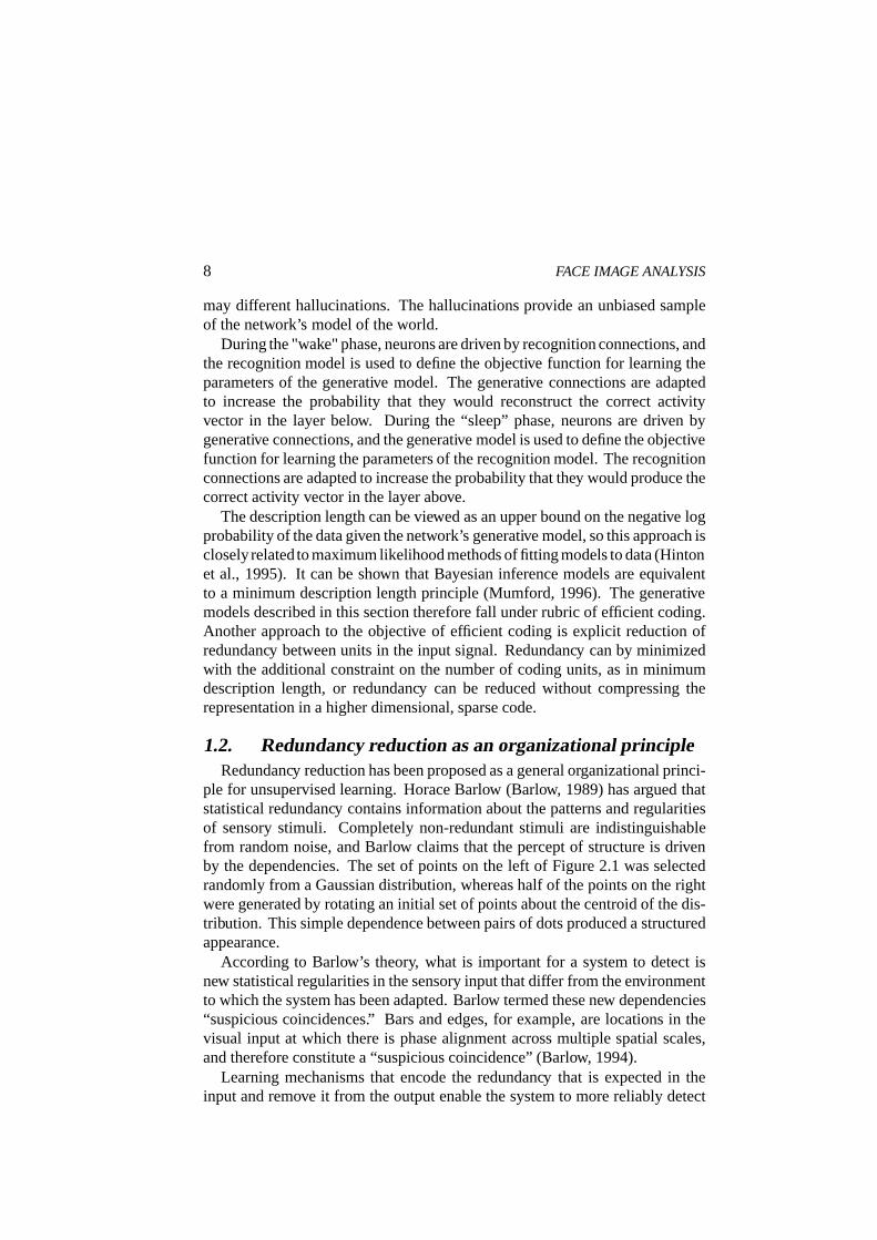
ple for unsupervised learning. Horace Barlow (Barlow, 1989) has argued thatstatistical redundancy contains information about the patterns and regularitiesof sensory stimuli. Completely non-redundant stimuli are indistinguishablefrom random noise, and Barlow claims that the percept of structure is drivenby the dependencies. The set of points on the left of Figure 2.1 was selectedrandomly from a Gaussian distribution, whereas half of the points on the rightwere generated by rotating an initial set of points about the centroid of the dis-tribution. This simple dependence between pairs of dots produced a structuredappearance.

According to Barlow’s theory, what is important for a system to detect isnew statistical regularities in the sensory input that differ from the environmentto which the system has been adapted. Barlow termed these new dependencies“suspicious coincidences.” Bars and edges, for example, are locations in thevisual input at which there is phase alignment across multiple spatial scales,and therefore constitute a “suspicious coincidence” (Barlow, 1994).

Learning mechanisms that encode the redundancy that is expected in theinput and remove it from the output enable the system to more reliably detect

Introduction 9

Figure 2.1. The percept of structure is driven by the dependencies. LEFT: A set of pointsselected from a Gaussian distribution. RIGHT: Half of the points were selected from a Gaussiandistribution, and the other half were generated by rotating the points QSR about the centroid of thedistribution. Figure inspired by Barlow (1989).

these new regularities. Learning such a transformation is equivalent to mod-eling the prior knowledge of the statistical dependencies in the input (Barlow,1989). Independent codes are advantageous for encoding complex objects thatare characterized by high order combinations of features because the priorprobability of any particular high order combination is low. Incoming sensorystimuli are automatically compared against the null hypothesis of statisticalindependence, and suspicious coincidences signaling a new causal factor canbe more reliably detected.

Barlow pointed to redundancy reduction at several levels of the visual system.Refer to Figure 2.2. A first-order redundancy is mean luminance. Adaptationmechanisms take advantage of this nonrandom feature by using it as an expectedvalue, and expressing values relative to it (Barlow, 1989). The variance, asecond-orderstatistic, is the luminancecontrast. Contrast appears to be encodedrelative to the local mean contrast, as evidenced by the “simultaneous contrast”illusion, and by contrast gain control mechanisms observed in V1 (Heeger,1992).

1.3. Information theoryBarlow proposed an organizational principle for unsupervised learning based

on information theory. The information provided by a given response isdefined as the number of bits required to communicate an event that has prob-ability

* �� under a distribution that is agreed upon by the sender and receiver(Shannon and Weaver, 1949):T �� F�8�VU.WAX�Y � * �� F� (2.6)


a.

b.

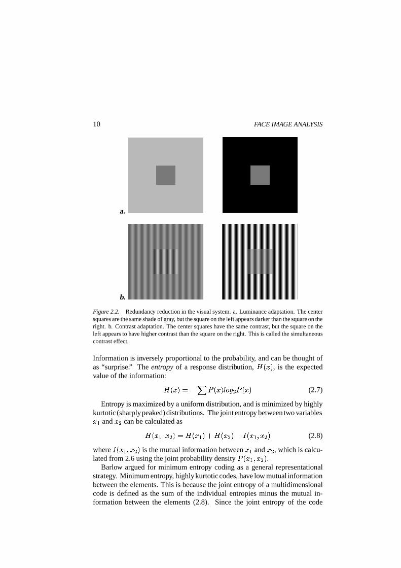
Figure 2.2. Redundancy reduction in the visual system. a. Luminance adaptation. The centersquares are the same shade of gray, but the square on the left appears darker than the square on theright. b. Contrast adaptation. The center squares have the same contrast, but the square on theleft appears to have higher contrast than the square on the right. This is called the simultaneouscontrast effect.

Information is inversely proportional to the probability, and can be thought ofas “surprise.” The entropy of a response distribution, Z[�� F� , is the expectedvalue of the information:Z[�� F��\U K * �� W�X]Y � * �� F� (2.7)

Entropy is maximized by a uniform distribution, and is minimized by highlykurtotic (sharplypeaked) distributions. The joint entropy between two variables � and � can be calculated asZ[�� E � �8�^Z[�� _[Z[�� 7U T �� E � � (2.8)

where

T �� E � � is the mutual information between � and � , which is calcu-lated from 2.6 using the joint probability density

* �� E � � .Barlow argued for minimum entropy coding as a general representational

strategy. Minimum entropy, highly kurtoticcodes, have low mutual informationbetween the elements. This is because the joint entropy of a multidimensionalcode is defined as the sum of the individual entropies minus the mutual in-formation between the elements (2.8). Since the joint entropy of the code

Introduction 11

stays constant, by minimizing the sum of the individual entropies, the mutualinformation term is also minimized. Another way to think of this is movingthe redundancy from between the elements to redundancy within the distribu-tions of the individual elements (Field, 1994). The distributions of individualelements with minimum entropy are redundant in the sense that they almostalways take on the same value.

Atick and Redlich (Atick and Redlich, 1992) approach the objective ofredundancy reduction from the perspective of efficient coding. They pointout that natural stimuli are very redundant, and hence the sample of signalsformed by an array of sensory receptors is inefficient. Atick (Atick, 1992)described evolutionary advantages of efficient coding such as coping withinformation bottlenecks due to limited bandwidth and limited dynamic range.Atick argued for the principle of efficiency of information representation as adesign principle for sensory coding, and presented examples from the blowflyand the mammalian retina.

1.4. Redundancy reduction in the visual systemThe large monopolar cells (LMC) in the blowfly compound eye eliminate

inefficiency due to unequal use of neural response levels (Laughlin, 1981). Themost efficient response gain is the one such that the probability distribution ofthe outputs is constant for all output states (maximum entropy). The solution isto match the gain of the transfer function to the cumulative probability densityof the input. Laughlin (Laughlin, 1981) measured the cumulative probabilitydensity of contrast in the fly’s environment, and found a close match betweenthe gain of the LMC neurons and the cumulative probability density function.

Atick made a similar argument for the modulation transfer function (MTF)of the mammalian retina. The cumulative density of the amplitude spectrumof natural scenes is approximately `�acb where b is frequency

�(Field, 1987).

The MTF makes an efficient code by equalizing the response distribution ofthe output over spatial frequency. Atick demonstrated that multiplying theexperimentally observed retinal MTF’s by `�acb produces an approximately flatoutput for frequencies less than 3 cycles per degree. Atick refers to such transferfunctions as whitening filters, since they equalize the response distribution ofthe output over all frequencies.

Macleod and von der Twer (Macleod and von der Twer, 1996) generalizedLaughlin’s analysis of optimal gain control to the presence of noise. In thenoiseless case, the gain that maximizes the information transfer is the one thatmatches the cumulative probability density of the input, but in the presence ofnoise, the optimal transfer function has a shallower slope in order to increase�

Spatial frequency is determined by a Fourier transform on the wave form defined by brightness as a functionof spatial position. In 2D images, a 1-D analysis is repeated at multiple orientations.


the signal-to-noise ratio. Macleod and von der Twer defined an optimal transferfunction for color coding, which they termed the “pleistochrome,” that max-imizes the quantity of distinguishable colors in the presence of output noise.The analysis addressed the case of a single input and output � , and used acriterion of minimum mean squared reconstruction error of the input, giventhe output plus output noise with variance � . The minimum squared errorcriterion performs principal component analysis which, as will be discussedin the next section, maximizes the entropy of the output for the single unitcase. In the presence of noise, the optimal transfer function was a gain propor-tional to �ed * �f �� g , which was less than the cumulative probablility density,and modulated by the amount of noise, � . Macleod and von der Twer foundthat the pleistochrome based on the distribution of cone responses along theh Ui�Aj6_lkN� axis � accounted well for the spectral sensitivity of the blue-yellowopponent channel observed at higher levels in the primate visual system.

These analyses have presented means for maximizing efficiency of codingfor a single input and output. Principal component analysis is a means ofreducing redundancies between multiple outputs. Atick and Redlich (Atickand Redlich, 1992) have argued for compact decorrelating mechanisms such asprincipal component analysis as a general coding strategy for the visual system.PCA decorrelates the input through an axis rotation. PCA provides a set of axesfor encoding the input in fewer dimensions with minimum loss of information,in the squared error sense. Principal component analysis is an example of acoding strategy that in Barlow’s formulation, encodes the correlations that areexpected in the input and removes them from the output.

1.5. Principal component analysisPrincipal component analysis (PCA) finds an orthonormal set of axes point-

ing in the directions of maximum covariance in the data. Let m be a datasetin which each column is an observation and each row is a measure with zeromean. The principal component axes are the eigenvectors of the covariancematrix of the measures,

�n memeo , where p is the number of observations. Thecorresponding eigenvalues indicate the proportion of variability in the data forwhich each eigenvector accounts. The first principal component points in thedirection of maximum variability, the second eigenvector points in the direc-tion of maximum variability orthogonal to the first, and so forth. The data arerecoded in terms of these axes by vector projection of each data point ontoeach of the new axes. Let

*be the matrix containing the principal component

eigenvectors in its columns. The PCA representation for each observation is

�Blue-yellow axis. S, M, and L stand for short, medium, and long wavelength selective cones. These

correspond roughly to blue, green, and red. L+M corresponds to yellow.

Introduction 13

obtained in the rows of q by

q��^m o * (2.9)

The eigenvectors in*

can be considered a set of weights on the data, m ,where the outputs are the coefficients in the matrix, q . Because the principalcomponent eigenvectors are orthonormal, they are also basis vectors for thedataset m . This is shown as follows: Since

*is symmetric and the columns

of*

are orthonormal,*:* o\� T

, where

Tis the identity matrix, and right

multiplication of 2.9 by* o gives q * o �0m . The original data can therefore

be reconstructed from the coefficients q using the eigenvectors in*

now asbasis vectors. A lower dimensional representation can be obtained by selectinga subset of the principal components with the highest eigenvalues, and it canbe shown that for a given number of dimensions, the principal componentrepresentation minimizes mean squared reconstruction error.

Because the eigenvectors point in orthogonal directions in covariance space,the principal component representation is uncorrelated. The coefficients forone of the axes cannot be linearly predicted from the coefficients of the otheraxes. Another way to think about the principal component representation isin terms of the generative models described in Section 1.1. PCA models thedata as a multivariate Gaussian where the covariance matrix is restricted to bediagonal. It can be shown that a generative model that maximizes the likelihoodof the data given a Gaussian with a diagonal covariance matrix is equivalentto minimizing mean squared error of the generated data. PCA can also beaccomplished through Hebbian learning, as described in the next section.

1.6. Hebbian learningHebbian learning is an unsupervised learning rule that was proposed as a

model for activity dependent modification of synaptic strengths between neu-rons (Hebb, 1949). The learning rule adjusts synaptic strengths in proportionto the activity of the pre and post-synaptic neurons. Because simultaneouslyactive inputs cooperate to produce activity in an output unit, Hebbian learningfinds the correlational structure in the input. See (Becker and Plumbley, 1996)for a review of Hebbian learning.

For a single output unit, it can be shown that Hebbian learning maximizesactivity variance of the output, subject to saturation bounds on each weight,and limits on the total connection strength to the output neuron (Linsker, 1988).Since the first principal component corresponds to the weight vector that maxi-mizes the variance of the output, then Hebbian learning, subject to the constraint


that the weight vector has unit length, is equivalent to the finding first principalcomponent of the input (Oja, 1982).

For a single output unit, � , where the activity of � is the weighted sum of theinput, �C�0/ �sr �A �� , the simple Hebbian learning algorithmt r � �^>7 � � (2.10)

with learning rate > will move the vector r �u" r � � $&$&$ � r ' ( towards the firstprincipal component of the input . In the simple learning algorithm, the lengthof r is unbounded. Oja modified this algorithm so that the length of r wasnormalized after each step. With a sufficiently small > , Hebbian learning withlength normalization is approximated byt r �^>7�F�� lU r �� $ (2.11)

This learning rule converges to the unit length principal component. The U r � �term tends to decease the length of r if it gets too large, while allowing it toincrease if it gets too small.

In the case of p output units, in which the p outputs are competing foractivity, Hebbian learningcan span the space of the first p principalcomponentsof the input. With the appropriate form of competition, the Hebb rule explicitlyrepresents the p principal components in the activities of the output layer (Oja,1989; Sanger, 1989). A learning rule for the weight r 5 to output unit � 5 thatexplicitly finds the first p principal components of the data ist r 5 �^>v� 5 �� lU r 5 � 5 _[w 5yx �Kzy{ � � (2.12)

The algorithm forces successive outputs to learn successive principal compo-nents of the data by subtracting estimates of the previous components from theinput before the connections to a given output unit are updated.

Linsker (Linsker, 1988) also demonstrated that for the case of a single outputunit, Hebbian learning maximizes the information transfer between the inputand the output. The Shannon information transfer rate| � T �� v�E��8�^Z[��<U}Z[��+ �� (2.13)

gives the amount of information that knowing the output � conveys about theinput , and is equivalent to the mutual information between them,

T �� v�E�� .For a single output unit � with a Gaussian distribution, 2.13 is maximized bymaximizing the variance of the output (Linsker, 1988). Maximizing outputvariance within the constraint of a Gaussian distribution produces a responsedistribution that is as flat as possible (i.e. high entropy). Maximizing output

Introduction 15

entropy with respect to a weight r maximizes 2.13, because the second term,Z~��+ F� , is noise and does not depend on r .Linsker argued for maximum information preservation as an organizational

principle for a layered perceptual system. There is no need for any higher layerto attempt to reconstruct the raw data from the summary received from thelayer below. The goal is to preserve as much information as possible in order toenable the higher layers to use environmental information to discriminate therelative value of different actions. In a series of simulations described later inthis chapter, in Section 3, Linsker (Linsker, 1986) demonstrated how structuredreceptive fields � with feature-analyzing properties related to the receptive fieldsobserved in the retina, LGN, and visual cortex could emerge from the principleof maximum information preservation. This demonstration was implementedusing a local learning rule� subject to constraints. Information maximiza-tion has recently been generalized to the multi-unit case (Bell and Sejnowski,1995). Information maximization in multiple units will be discussed below inSection 2. This monograph examines representations for face images based oninformation maximization.

1.7. Learning rules for explicit discovery of statisticaldependencies

A perceptual system can be organized around internally derived teachingsignals generated from the assumption that different parts of the perceptualinput have common causes in the external world. One assumption is that thevisual input is derived from physical sources that are approximately constantover space. For example, depth tends to vary slowly over most of the visualinput except at object boundaries. Learning algorithms that explicitly encodestatistical dependencies in the input attempt to discover those constancies. Theactual output of such invariance detectors represents the extent to which thecurrent input violates the network’s model of the regularities in the world(Becker and Plumbley, 1996). The Hebbian learning mechanism described inthe previous section is one means for encoding the second order dependencies(correlations) in the input.

The GMAX algorithm (Pearlmutter and Hinton, 1986) is a learning rule formultiple inputs to a single output unit that is based on the goal of redundancyreduction. The algorithm compares the response distribution,

*of the output

unit to the response distribution, M , that would be expected if the input wasfA receptive field of a neuron is the input that influences its activity rate. Many neurons in the retina and

lateral geniculate nucleus of the thalamus (LGN) have receptive fields with excitatory centers and inhibitorysurrounds. These respond best to a spot of light surrounded by a dark annulus at a particular location in thevisual field. Many neurons in the primary visual cortex respond best to oriented bars or edges.�

Local learning rules may be more biologically plausible than rules that evaluate information from all units,given the limited extent of synaptic connections


entirely independent. The learning algorithm causes the unit to discover thestatistical dependencies in the input by maximizing the difference between

*and M .

*is determined by the responses to the full set of data under the current

weight configuration, and M can be calculated explicitly by sampling all of thew ' possible states of the input units. The GMAX learning rule is limited tothe case of a single output unit, and probabilistic binary units.

Becker (Becker, 1992) generalized GMAX to continuous inputs with Gaus-sian distributions. This resulted in a learning rule that minimized the ratio ofthe output variance to the variance that would be expected if the input lineswere independent. This learning rule discovers statistical dependencies in theinput, and is literally an invariance detector. If we assume that properties ofthe visual input are derived from constant physical sources, then a learningrule that minimizes the variance of the output will tell us something aboutthat physical source. Becker further generalized this algorithm to the case ofmultiple output units. These output units formed a mixture model of differentinvariant properties of the input patterns.

Becker and Hinton (Becker and Hinton, 1992; Becker and Hinton, 1993)applied the multi-unit version of this learning rule to show how internallyderived teaching signals for a perceptual system can be generated from theassumption that different parts of the perceptual input have common causesin the external world. In their learning scheme, small modules that look atseparate but related parts of the perceptual input discover these common causesby striving to produceoutputs that agree with each other. The modules may lookat different modalities such as vision and touch, or the same modality at differenttimes, such as the consecutive two-dimensional views of a rotating three-dimensional object, or spatially adjacent parts of the same image. The learningrule, which they termed IMAX, maximizes the mutual information betweenpairs of output units, �� and �� . Under the assumption that the two output unitsare caused by a common underlying signal corrupted by independent Gaussiannoise, then the mutual information between the underlying signal and the meanof � � and �� is given by T �^� $�� WAX]YG� �� _�� U�� (2.14)

where � is the variance function over the training cases. The algorithm canbe understood as follows: A simple way to make the outputs of the twomodules agree is to use the squared difference between the module outputs asa cost function (the denominator of 2.14). A minimum squared difference costfunction alone, however will cause both modules to produce the same constantoutput that is unaffected by the input, and thereforeconvey no information aboutthe input. The numerator modified the cost function to minimize the squareddifference relative to how much both modules varied as the input varied. This

Introduction 17

forced the modules to respond to something that was common in their twoinputs.

Becker and Hinton showed that maximizing the mutual information be-tween spatially adjacent parts of an image can discover depth in random dotstereograms of curved surfaces. The simulation consisted of a pair of 2-layernetworks, each with a single output unit, that took spatially distinct regionsof the visual space as input. The input consisted of random dot stereogramswith smoothly varying stereo disparity. Following training, the module outputswere proportional to depth, despite no prior knowledge of the third dimen-sion. The model was extended to develop population codes for stereo disparity(Becker and Hinton, 1992), and to model the locations of discontinuities indepth (Becker, 1993).

Schraudolph and Sejnowski (Schraudolph and Sejnowski, 1992) proposedan algorithm for learning invariances that was closely related to Becker andHinton’s constrained variance minimization. They combined a variance-minimizing anti-Hebbian term, in which connection strengths are reduced inproportion to the pre-and post synaptic unit activities, with a term that preventedthe weights from converging to zero. They showed that a set of competing unitscould discover population codes for stereo disparity in random dot stereograms.

Zemel and Hinton (Zemel and Hinton, 1991) applied the IMAX algorithm tothe problem of learning to represent the viewing parameters of simple objects,such as the object’s scale, location, and size. The algorithm attempts to learnmultiple features of a local image patch that are uncorrelated with each other,while being good predictors of the feature vectors extracted from spatiallyadjacent input locations. The algorithm is potentially more powerful thanlinear decorrelating methods such as principal component analysis because itcombines the objective of decorrelating the feature vector with the objective offinding common causes in the spatial domain. Extension of the algorithm tomore complex inputs than synthetic 2-D objects is limited, however, due to thedifficulty of computing the determinants of ill-conditioned matrices (Beckerand Plumbley, 1996).

2. INDEPENDENT COMPONENT ANALYSIS2.1. Decorrelation versus independence

Principal component analysis decorrelates the input data, but does not ad-dress the high-order dependencies. Decorrelation simply means that variablescannot be predicted from each other using a linear predictor. There can stillbe nonlinear dependencies between them. Consider two variables, and � thatare related to each other by a sine wave function, �C�� F� . The correlationcoefficient for the variables and � would be zero, but the two variables arehighly dependent nonetheless. Edges, defined by phase alignment at multiple


spatial scales, are an example of a high-order dependency in an image, as areelements of shape end curvature.

Second-order statistics capture the amplitude spectrum of images but not thephase (Field, 1994). Amplitude is a second-order statistic. The amplitude spec-trum of a signal is essentially a series of correlations with a set of sine-waves.Also, the Fourier transform of the autocorrelation function of a signal is equalto its power spectrum (square of the amplitude spectrum). Hence the amplitudespectrum and the autocorrelation function contain the same information. Theremaining information that is not captured by the autocorrelation function, thehigh order statistics, corresponds to the phase spectrum.�

Coding mechanisms that are sensitive to phase are important for organizing aperceptual system. Spatial phase contains the structural information in imagesthat drives human recognition much more strongly than the amplitude spectrum(Oppenheim and Lim, 1981; Piotrowski and Campbell, 1982). For example, Aface image synthesized from the amplitude spectrum of face A and the phasespectrum of face B will be perceived as an image of face B.

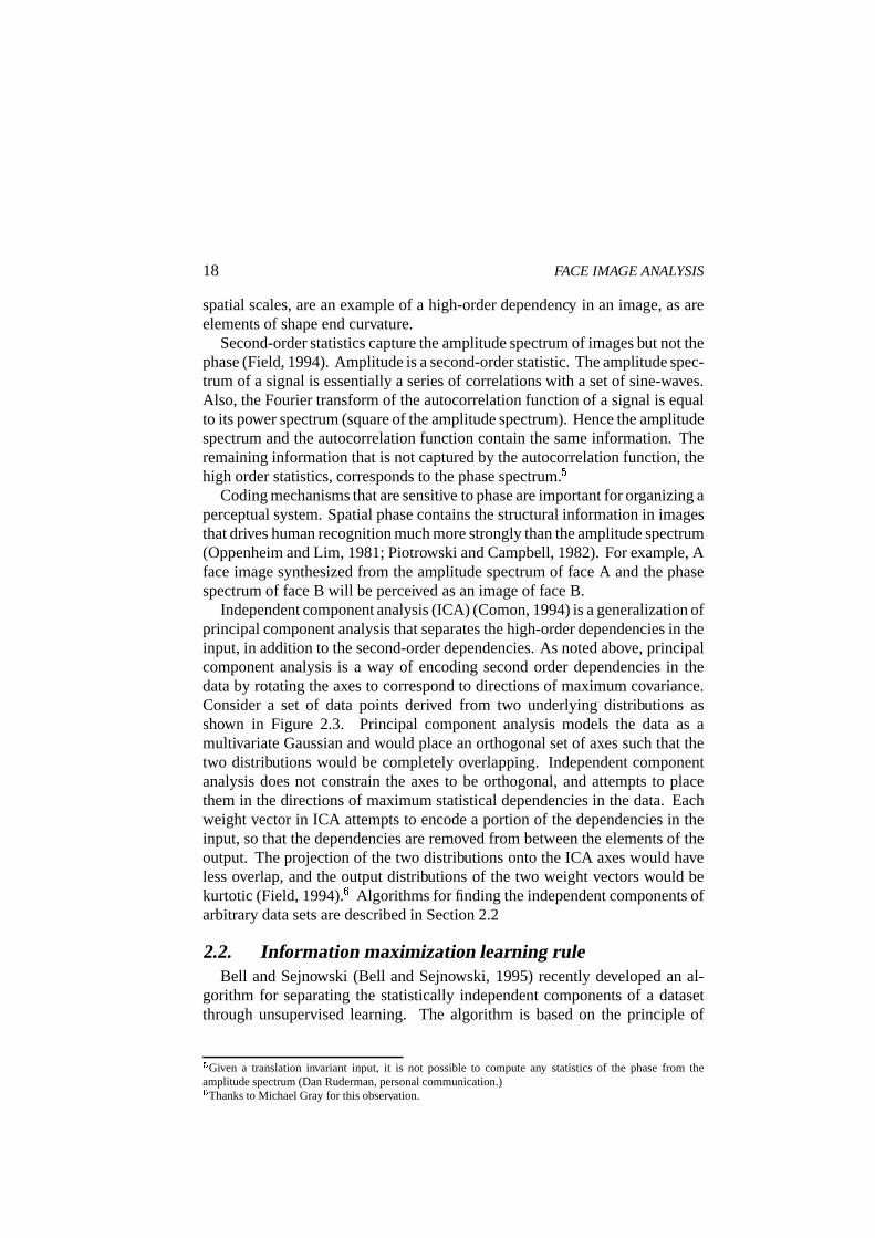
Independent component analysis (ICA) (Comon, 1994) is a generalization ofprincipal component analysis that separates the high-order dependencies in theinput, in addition to the second-order dependencies. As noted above, principalcomponent analysis is a way of encoding second order dependencies in thedata by rotating the axes to correspond to directions of maximum covariance.Consider a set of data points derived from two underlying distributions asshown in Figure 2.3. Principal component analysis models the data as amultivariate Gaussian and would place an orthogonal set of axes such that thetwo distributions would be completely overlapping. Independent componentanalysis does not constrain the axes to be orthogonal, and attempts to placethem in the directions of maximum statistical dependencies in the data. Eachweight vector in ICA attempts to encode a portion of the dependencies in theinput, so that the dependencies are removed from between the elements of theoutput. The projection of the two distributions onto the ICA axes would haveless overlap, and the output distributions of the two weight vectors would bekurtotic (Field, 1994).� Algorithms for finding the independent components ofarbitrary data sets are described in Section 2.2

2.2. Information maximization learning ruleBell and Sejnowski (Bell and Sejnowski, 1995) recently developed an al-

gorithm for separating the statistically independent components of a datasetthrough unsupervised learning. The algorithm is based on the principle of�

Given a translation invariant input, it is not possible to compute any statistics of the phase from theamplitude spectrum (Dan Ruderman, personal communication.)�

Thanks to Michael Gray for this observation.

Introduction 19

•

•

•

•

•

•

•

••

•

••

•

•

•

•

•

•

•

•

••

•

•

•

•

•

••

•

•

•

•

•

•

••

•

••

•

•

•

•

•

•••

•

•

•

• •

•

•

•

•

•

••

••

••

•

•

•

•

•

•

•

•

•

•

••

• •

•

•

•

•• ••

•

••

•

•

• •••

•

�6��•

• •

•

•

•

•

•

•

••

•

••

•

•

•

•

•

•

•

•

••

•

•

•

•

•

••

•

•

•

•

•

•

••

•

••

•

•

•

•

•

•••

•

•

•

• •

•

•

•

•

•

••

••

••

•

•

•

•

•

•

•

•

•

•

••

• •

•

•

•

•• ••

•

••

•

•

• •••

•

��•

Figure 2.3. Example 2-D data distribution and the corresponding principal component andindependent component axes. The data points could be, for example, grayvalues at pixel 1 andpixel 2. Figure inspired by Lewicki & Sejnowski (2000).

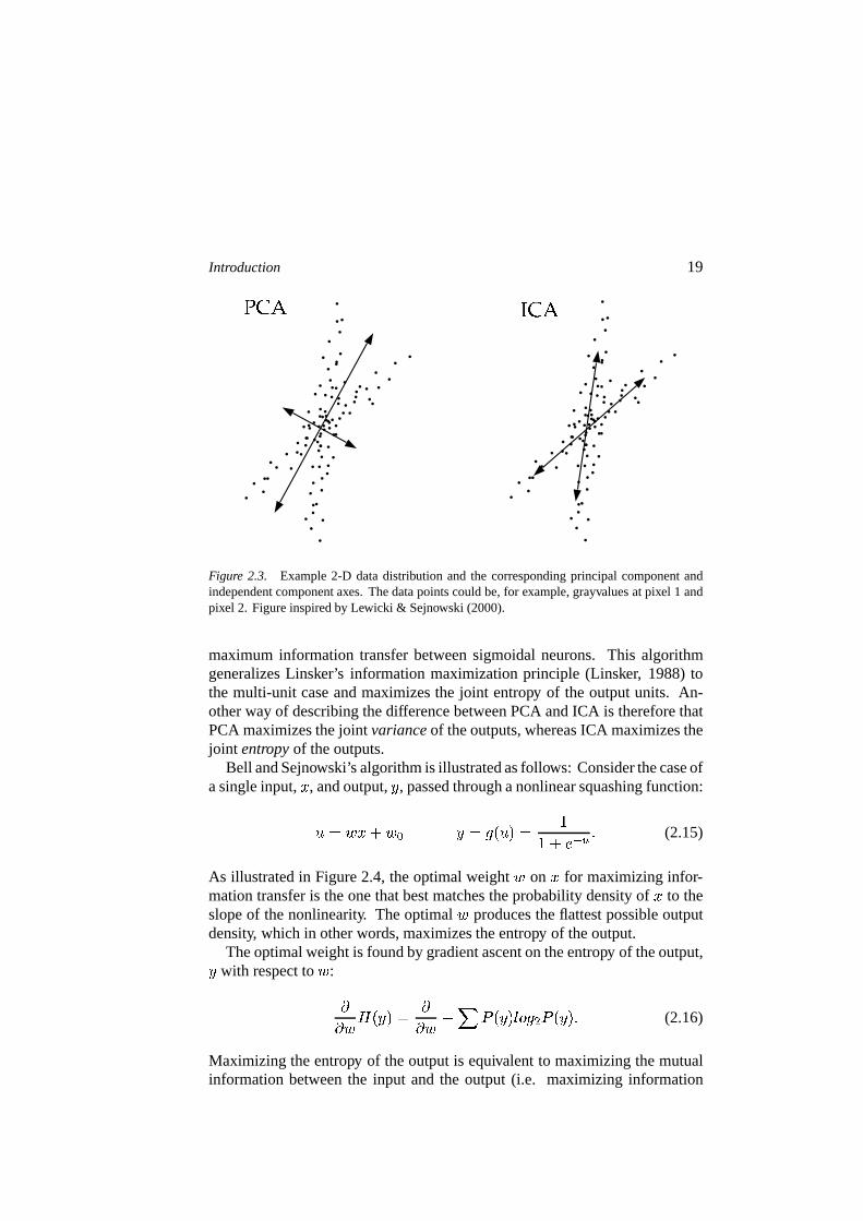
maximum information transfer between sigmoidal neurons. This algorithmgeneralizes Linsker’s information maximization principle (Linsker, 1988) tothe multi-unit case and maximizes the joint entropy of the output units. An-other way of describing the difference between PCA and ICA is therefore thatPCA maximizes the joint variance of the outputs, whereas ICA maximizes thejoint entropy of the outputs.

Bell and Sejnowski’s algorithm is illustrated as follows: Consider the case ofa single input, , and output, � , passed through a nonlinear squashing function:

�i� r �_ r9� �C��Y��F�� ``,_!� x�� $ (2.15)

As illustrated in Figure 2.4, the optimal weight r on for maximizing infor-mation transfer is the one that best matches the probability density of to theslope of the nonlinearity. The optimal r produces the flattest possible outputdensity, which in other words, maximizes the entropy of the output.

The optimal weight is found by gradient ascent on the entropy of the output,� with respect to r : �� r Z~��8�� r U[K * ��WAX]Y � * �� $ (2.16)

Maximizing the entropy of the output is equivalent to maximizing the mutualinformation between the input and the output (i.e. maximizing information

20 FACE IMAGE ANALYSIS�

�� J¡¢£¥¤¦@§ ¨ª©�«�¬

¤

«®

1 ¯±°³² ©�«�¬«

1

´

µ[¶�·ª¸¹

¹ººi»c¼�½ ¾

¿¿À

Á¾Â

Figure 2.4. Optimal information flow in sigmoidal neurons. The input Ã is passed througha nonlinear function, Ä�Å&Ã�Æ . The information in the output density Ç�È�Å&É]Æ depends on matchingthe mean and variance of Ç�ÊsÅ&Ã�Æ to the slope and threshold of Ä�Å&ÃËÆ . Right: Ç È Å&ÉsÆ is plotted fordifferent values of the weight, Ì . The optimal weight, Ì�ÍAÎEÏ transmits the most information.Figure from Bell & Sejnowski (1995), reprinted with permission from MIT Press, copyright1995, MIT Press.

transfer). This is because

T �� 7�E��^Z~�� Ë_ÐZ[��ÑU@Z[��+ F� , where only Z[��depends on the weight r since Z[��+ �� is noise.

When there are multiple inputs and outputs, mÒ�Ó�� E � � $&$&$ � , ÔV�Ó�� E� � �$&$&$ � maximizing the joint entropy of the output encourages the individual out-puts to move towards statistical independence. To see this, we refer back toEquation 2.8: Z~�� E� � �D�^Z[�� _±Z[�� U T �� E� � � . Maximizing the jointentropy of the output Z[�� E� � � $&$&$ � encourages the mutual information betweenthe individual outputs

T �� E� � � $&$&$ � to be small. The mutual information is guar-anteed to reach a minimum when the nonlinear transfer function Y matches thecumulative distribution of the independent signals responsible for the data in , up to scaling and translation (Nadal and Parga, 1994; Bell and Sejnowski,1997). Many natural signals, such as sound sources, have been shown to havea super-Gaussian distribution, meaning that the kurtosis of the probability dis-tribution exceeds that of a Gaussian (Bell and Sejnowski, 1995). For mixturesof super-Gaussian signals, the logistic transfer function has been found to besufficient to separate the signals (Bell and Sejnowski, 1995).

Since �Ð�\Y�� F� and Y is monotonic, the probability* �� in Equation 2.16

can be written in terms of* �� F� in the single unit case as (Papoulis, 1991)* ��D�ÖÕ<×ÙØ�ÚÛ ÈÛ Ê and in the multiunit case as

* �AÔ��D�ÜÕ<×ÙÝOÚÞ ßJÞwhere +�à,+ is the determinant of the Jacobian, à . à is the matrix of partialderivatives áyâ�ãá Ø ã . Hence

Introduction 21

Z[�AÔ��8�\U Håä WAX�Y � * ��m��+�à,+±æ �çZ[��mè�7_ H �2WAX]Y � +�à,+é� $ (2.17)Since Z~��m�� does not depend on ê , the problem reduces to maximizing +�à,+with respect to ê . Computing the gradient of +�à,+ with respect to ê results inthe following learning rule: ët êì�^>±dc�ê o � x � _~�JíÙ o g (2.18)

where � í � ááyâ�ã áyâ�ãá � ã � áá � ã W� áyâ�ãá � ã $Bell & Sejnowski improved the algorithm in 1997 by using the natural

gradient (Amari et al., 1996). They multiplied the gradient equation by thesymmetric matrix ê o ê which removed the inverse and scaled the gradientdifferently along different dimensions. The natural gradient addresses the prob-lem that the metric space of W is not necessarily Euclidean. Each dimensionhas its own scale and the natural gradient normalizes the metric function forthat space. This resulted in the following learning rule:t êî�^>P� T _��Ñíï o ê o �Eê (2.19)

Although it appears at first contradictory, information maximization in amultidimensional code is consistent with Barlow’s notion of minimum entropycoding. Refer again to Equation 2.8. As noted above, maximizing the jointentropy of the output encourages the mutual information between the outputsto be small, but under some conditions other solutions are possible for whichthe mutual information is nonzero. Given that the joint entropy stays constant(at its maximum), the solution that minimizes the mutual information will alsominimize the marginal (individual) entropies of the output units.

An application of independent component analysis is signal separation. Mix-tures of independent signals can be separated by a weight matrix that minimizesthe mutual information between the outputs of the transformation. Bell & Se-jnowski’s information maximization algorithm successfully solved the “cock-tail party” problem, in which a set random mixtures of auditory signals wereseparated without prior knowledge of the original signals or the mixing process(Bell and Sejnowski, 1995). The algorithm has also been applied to separatingthe sources of EEG signals (Makeig et al., 1996), and fMRI images (McKeownet al., 1998).

Independent component analysis can be considered as a generative model ofthe data assuming independent sources. Each data point is assumed to be alinear mixture of independent sources, ð�^qñ� , where q is a mixing matrix, andò

The step from 2.17 to 2.18 is presented in the Appendix of (Bell and Sejnowski, 1995).

22 FACE IMAGE ANALYSIS� contains the sources. Indeed, a maximum likelihood approach for findingq and � can be shown to be mathematically equivalent to the informationmaximization approach of Bell and Sejnowski (MacKay, 1996; Pearlmutterand Parra, 1996). In the maximum likelihood approach, a likelihood functionof the data is generated under the model ð�^qñ� , where the probabilities of thesources � are assumed to be factorial. The elements of the basis matrix q andthe sources � are then obtained by gradient ascent on the log likelihood function.Another approach to independent component analysis involves cost functionsusing marginal cumulants (Comon, 1994; Cardoso and Laheld, 1996). Theadaptive methods in the information maximization approach are more plausiblefrom a neural processing perspective than the cumulant-based cost functions(Lee, 1998).

A large variety of algorithms have been developed to address issues includ-ing extending the information maximization approach to handle sub-Gaussiansources (Lee et al., 1999), estimating the shape of the distribution of inputsources with maximum likelihood techniques (Pearlmutter and Parra, 1996),nonlinear independent component analysis (Yang et al., 1998), and biolog-ically inspired algorithms that perform ICA using local computations (Linet al., 1997). I refer you to (Lee, 1998) for a thorough review of algorithms forindependent component analysis.

2.3. Relation of sparse coding to independenceAtick argued for compact, decorrelated codes such as PCA because of ef-

ficiency of coding. Field (Field, 1994) argued for sparse, distributed codesin favor of such compact codes. Sparse representations are characterized byhighly kurtotic response distributions, in which a large concentration of valuesare near zero, with rare occurrences of large positive or negative values inthe tails. Recall that highly kurtotic response distributions have low entropy.Maximizing sparseness of a response distribution is related to minimizing itsentropy, and sparse codes therefore incur the same advantages as minimumentropy codes, such as separation of high-order redundancies in addition to thesecond-order redundancy. In such a code, the redundancy between the elementsof the input is transformed into redundancy within the response patterns of theindividual outputs, where the individual outputs almost always give the sameresponse except on rare occasions.

Given this relationship between sparse codes and minimum entropy, theadvantages of sparse codes as outlined in (Field, 1994) are also arguments infavor of Barlow’s minimum entropy codes (Barlow, 1989). Codes that minimizethe number of active neurons can be useful in the detection of suspiciouscoincidences. Because a nonzero response of each unit is relatively rare, highorder relations become increasingly rare, and therefore more informative whenthey are present in the stimulus. Field contrasts this with a compact code

Introduction 23

such as principal components, in which a few cells have a relatively highprobability of response, and therefore high order combinations among thisgroup are relatively common. In a sparse distributed code, different objectsare represented by which units are active, rather than by their rate of activity.These representations have an added advantage in signal-to-noise, since oneneed only determine which units are active without regard to the precise levelof activity. An additional advantage of sparse coding for face representations isstorage in associative memory systems. Networks with sparse inputs can storemore memories and provide more effective retrieval with partial information(Palm, 1980; Baum et al., 1988).

Field presented evidence that oriented Gabor filters produce sparse codeswhen presented with natural scenes, whereas the response distribution is Gaus-sian when presented with synthetic images generated from `�acb noise. Becausethe two image classes had the same amplitude spectra and differed only inphase, Field concluded that sparse coding by Gabor filters depends primarilyon the phase spectra of the data. Olshausen and Field (Olshausen and Field,1996b; Olshausen and Field, 1996a) showed that a generative model with asparseness objective can account for receptive fields observed in the primaryvisual cortex. They trained a network to reconstruct natural images from a lin-ear combination of unknown basis images with minimum mean-squared error.The minimum squared error criterion alone would have converged on a linearcombination of the principal components of the images. When a sparsenesscriterion was added to the objective function, the learned basis images werelocal, oriented, and spatially opponent, similar to the response properties ofV1 simple cells. ó Maximizing sparseness under the constraint of informationpreservation is equivalent to minimum entropy coding.

Bell & Sejnowski also examined an image synthesis model of natural scenesusing independent component analysis (Bell and Sejnowski, 1997). As ex-pected given the relationship between sparse coding and independence, Bell &Sejnowski obtained a similar result to Olshausen and Field, namely the emer-gence of local, spatially opponent receptive fields. Moreover, the responsedistributions of the individual output units were indeed sparse. Decorrelationmechanisms such as principal components resulted in spatially opponent re-ceptive fields, some of which were oriented, but were not spatially local. Inaddition, the response distributions of the individual PCA output units wereGaussian. In a related study, Wachtler, Lee, and Sejnowski (Wachtler et al.,2001) performed ICA on chromatic images of natural scenes. Redundancy re-duction was much higher in the chromatic case than in the grayscale case. The

ô“Simple cells” in the primary visual cortex respond to an oriented bar at a precise location in the visual

field. There is a surrounding inhibitory region, such that the receptive field is similar to a sine wave gratingmodulated by a Gaussian.


resulting filters segmented into color opponent and broadband filters, parallel-ing the color opponent and broadband channels in the primate visual system.These filters had very sparse distributions, suggesting that color opponency inthe human visual system achieves a highly efficient representation of colors.

3. UNSUPERVISED LEARNING IN VISUALDEVELOPMENT

3.1. Learning input dependencies: Biological evidenceThere is a large body of evidence that self-organization plays a considerable

role in the development of the visual system, and that this self-organizationis mediated by learning mechanisms that are sensitive to dependencies in theinput. The gross organization of the visual system appears to be governedby molecular specificity mechanisms during embryogenesis (Harris and Holt,1990). Such processes as the generation of the appropriate numbers of targetneurons, migration to the appropriate position, the outgrowth of axons, theirnavigation along appropriate pathways, recognition of the target structure, andthe formation of at least coarsely defined topographic maps õ may be mediatedby molecular specificity. During postnatal development, the architecture of thevisual system continues to become defined, organizing into ocular dominanceand orientation columns.

� � The statistical properties of early visual experienceand endogenous activity appear to be responsible for shaping this architecture.See (Stryker, 1991a) for a review.

Learning mechanisms that are sensitive to dependencies in the visual inputtransform these statistical properties into cortical receptive field architecture.The NMDA receptor could be the “correlation detector” for Hebbian learningbetween neurons. It opens calcium channels in the post synaptic cell in amanner that depends on activity in both the pre- and the post-synaptic cell.Specifically, it depends on glutamate from the presynaptic cell and the voltageof the post synaptic cell. Although it is not known exactly how activationof the NMDA receptor would lead to alterations in synaptic strength, severaltheories have been put forward involving the release of trophic substances,retrograde messenger systems leading back to the presynaptic neuron, andsynaptic morphology changes (Rison and Stanton, 1995).

Visual development appears to be closely associated with NMDA gating(Constantine-Paton et al., 1990). There is longer NMDA gating during visualdevelopment, which provides a longer temporal window for associations. Lev-els of NMDA are high early in development, and then drop (Carmignoto and

öNeighboring neurons tend to respond to neighboring regions of the visual field.�¥÷Adjacent neurons in the primary visual cortex prefer gradually varying orientations. Perpendicular to this

are iso-orientation stripes. Eye preference is also organized into stripes.

Introduction 25

Vicini, 1992). These changes in NMDA activity appear to be dependent onexperience rather than age. Dark rearing will delay the drop in NMDA levels,and the decrease in length of NMDA gating is also dependent on activity (Foxet al., 1992).

The organization of ocular dominance and orientation preference can bealtered by manipulating visual experience. Monocular deprivation causes agreater proportion of neurons to prefer the active eye at the expense of thedeprived eye (Hubel et al., 1977). Colin Blakemore (Blakemore, 1991) foundthat in kittens reared in an environment consisting entirely of vertical stripes,orientation preference in V1 was predominantly vertical. The segregationof ocular dominance columns is dependent on both pre- and post-synapticactivity. Ocular dominance columns do not form when all impulse activityin the optic nerve is blocked by injecting tetrodotoxin (Stryker and Harris,1986). Blocking post-synaptic activity during monocular deprivation nulls theusual shift in ocular dominance (Singer, 1990; Gu and Singer, 1993). Strykerdemonstrated that ocular dominance segregation depends on asynchronous ac-tivity in the two eyes (Stryker, 1991a). With normal activity blocked, Strykerstimulated both optic nerves with electrodes. When the two nerve were stim-ulated synchronously, ocular dominance columns did not form, but when theywere stimulated asynchronously, columns did form. Consistent with the roleof NMDA in the formation of ocular dominance columns, NMDA receptorantagonists prevented the formation of ocular dominance columns, whereas in-creased levels of NMDA sharpened ocular dominance columns (Debinski et al.,1990). Some of organization of ocular dominance and orientation preferencedoes occur prenatally. Endogenous activity can account for the segregationof ocular dominance in the lateral geniculate nucleus (Antonini and Stryker,1993), and endogenous activity tends to be correlated in neighboring retinalganglion cells (Mastronarde, 1989).

Intrinsic horizontal axon collaterals in the striate cortex of adult cats specif-ically link columns having the same preferred orientation. Calloway and Katz(Callaway and Katz, 1991) demonstrated that the orientation specificity ofthese horizontal connections was dependent on correlated activity from view-ing sharply oriented visual stimuli. Crude clustering of horizontal axon collat-erals is normally observed in the striate cortex of kittens prior to eye opening.Binocular deprivation beyond this stage dramatically affected the refinementof these clusters. Visual experience appears to have been necessary for addingand eliminating collaterals in order to produce the sharply tuned specificitynormally observed in the adult.


3.2. Models of receptive field development based oncorrelation sensitive learning mechanisms

Orientation columns are developed prenatally in macaque. Therefore anyaccount of their development must not depend on visual experience. Linsker(Linsker, 1986) demonstrated that orientation columns can arise from ran-dom input activity in a layered system using Hebbian learning. The onlyrequirements for this system were arborization functions that were more densecentrally, specification of initial ratios of excitatory and inhibitory connections,and adjustment of parameters controlling the total synaptic strength to a unit.Because of the dense central connections, the random activity in the first layerbecame locally correlated in the second layer. Manipulation of the parameterfor total synaptic strength in the third layer brought on center-surround receptivefields. This occurred because of the competitive advantage of the dense cen-tral connections over the sparse peripheral connections. Activity in the centralregion became saturated first, and because of the bounds on activity, the periph-eral region became inhibitory. The autocorrelation function for activity in layer3 was Mexican hat shaped. Linsker added four more layers to the network. Thefirst three of these layers also developed center-surround receptive fields. Theeffect of adding these layers was to sharpen the Mexican hat autocorrelationfunction with each layer. Linsker associated the four center-surround layers ofhis model to the bipolar, retinal ganglion, LGN, and layer 4c cells in the visualsystem. A criticism of this section of Linsker’s model is that it predicts thatthe autocorrelation function in these layers should become progressively moresharply Mexican hat shaped, which does not appear to occur in the primatevisual system.

In the next layers of the model, Linsker demonstrated the development oforientation selective cells and their organization into orientation columns. Cellsreceiving inputs with a Mexican hat shaped autocorrelation function attemptedto organize their receptive fields into banded excitatory and inhibitory regions.By adjusting the parameter for total synaptic strength in layer seven, Linskerwas able to generate oriented receptive fields. Linsker subsequently gener-ated iso-orientation bands by adding lateral connections in the top layer. Thelateral connections were also updated by a Hebbian learning rule. Activityin like-oriented cells is correlated when the cells are aligned along the axisof orientation preference, but are anticorrelated on an axis perpendicular tothe preferred orientation. The lateral connections thus encourage the sameorientation along the axis of preferred orientation, and an orthogonal orienta-tion preferences along the axis orthogonal to the preferred orientation. Thisorganization resembles the singularities in orientation preference reported byObermayer and Blasdel (Obermayer and Blasdel, 1993). In Linsker’s model,

Introduction 27

a linear progression of orientation preference would require an isotropic auto-correlation function.

Miller, Keller, and Stryker (Miller et al., 1989) demonstrated that Hebbianlearning mechanisms can account for the development of ocular dominanceslabs and for experience-related alterations of this organization. In their model,synaptic strength was altered as a function of pre and post synaptic activity,where synaptic strength depended on within-eye and between-eye correla-tion functions. The model also contained constraints on the overall synapticstrength, an arborization function indicating the initial patterns of connectivity,and lateral connections between the cortical cells. All input connections wereexcitatory.

Miller et al. found that there were three conditions necessary for the de-velopment of ocular dominance columns. 1. The input activity must favormonocularity by having larger within-eye correlations than between-eye cor-relations. 2. There must be locally excitatory cortical connections. 3. If theintracortical connections are not Mexican hat shaped, in other words if theydo not have an inhibitory zone, then there must be a constraint on the totalsynaptic strength of the afferent axons. The ocular dominance stripes arosebecause of the intracortical activation function. If this function is Mexican hatshaped, then each cell will want to be in an island of like ocularity surroundedby opposite ocularity. Optimizing this force along a surface of cells resultsin a banded pattern of ocular dominance. The intracortical activation functioncontrols the periodicity of the stripes. The ocular dominance stripes will havea periodicity equal to the fundamental frequency of the intracortical activationfunction. This will be the case up to the limit of the arborization function. Ifthe excitatory region of the intracortical activation function is larger than thearborization function, then the periodicity of the stripes will be imposed by thearborization function.

Miller et al. found that a very small within-eye correlation function wassufficient to create ocular dominance stripes, so long as it was larger than thebetween eye correlation. Anticorrelation within an eye decreases monocularity,whereas anticorrelation between eyes, such as occurs in conditions of strabis-mus and monocular deprivation, increases monocularity. They also observedan effect related to critical periods. Monocular cells would remain stabilizedonce formed, and binocular cells would also stabilize if the synapses wereat saturating strength. Therefore, alterations could only be made while therewere still binocular cells with unsaturated connections. Due to the dependenceof ocular dominance on excitatory intracortical connections, their simulation


predicted that ocular dominance organization in the developing brain would beeliminated by increasing inhibition

�E�.

Berns, Dayan, and Sejnowski (Berns et al., 1993) presented a Hebbian learn-ing model for the development of both monocular and binocular populations ofcells. The model is driven by correlated activity in retinal ganglion cells withineach eye before birth, and between eyes after birth. An initial phase of same-eye correlations, followed by a second phase that included correlations betweenthe eyes produced a relationship between ocular dominance and disparity thathas been observed in the visual cortex of the cat. The binocular cells tendedto be selective for zero disparity, whereas the more monocular cells tended tohave nonzero disparity.

Obermayer, Blasdel, and Schulten (Obermayer et al., 1992) modeled thesimultaneous development of ocular dominance and orientation columns witha Kohonen self-organizing topographic map. This algorithm predicts the ob-served geometrical relations between ocular dominance and orientation pref-erence on the surface of the primary visual cortex. These include the per-pendicular iso-orientation slabs in the binocular regions, and singularities inorientation preference at the centers of highly monocular zones. According totheir model, cortical geometry is a result of projecting five features onto a twodimensional surface. The five features are spatial position along the horizon-taland vertical axes, orientation preference, orientation specificity, and oculardominance. The Kohonen self organizing map operates in the following way.The weights of the network attempt to learn a mapping from a five dimensionalinput vector onto a 2-D grid. The weight associated with each point on thegrid is the combination of the five features preferred by that unit. The unitwith the most similar weight vector to a given input vector, as measured bythe dot product, adjusts its weight vector toward the input vector. Neighboringunits on the grid also learn by a smaller amount according to a neighborhoodfunction. At the beginning of training, the "temperature" is set to a high level,meaning that the neighborhood function is broad and the learning rate is high.The temperature is gradually reduced during training. The overall effect of thisprocedure is to force units on the grid to vary their preferences smoothly andcontinuously, subject to the input probabilities. Like Hebbian learning, the selforganizing map creates structure from the correlations in input patterns, butthe self organizing map has the added feature that the weights are forced to besmooth and continuous over space.

Obermayer, Blasdel, and Schulten likened the development of cortical geom-etry to a Markov random process. There are several possible states of corticalgeometry, and the statistical structure of the input vectors trigger the transitionsbetween states. They showed that a columnar system will not develop if the�2�

e.g. through application of muscimol, A GABA agonist, where GABA is an inhibitory neurotransmitter

Introduction 29

input patterns are highly similar with respect to orientation preference, speci-ficity, and ocular dominance. Nor will it segregate into columns if the inputs areentirely uncorrelated. There is a range of input correlations for which colum-nar organization will appear. Their model predicts that ocular dominance andorientation columns will be geometrically unrelated in animals that are rearedwith an orientation bias in one eye.

4. LEARNING INVARIANCES FROM TEMPORALDEPENDENCIES IN THE INPUT

The input to the visual system contains not only spatial redundancies, buttemporal redundancies as well. There are several synaptic mechanisms thatmight depend on the correlation between synaptic input at one moment, andpost-synaptic depolarization at a later moment. Coding principles that aresensitive to temporal as well as spatial redundancies in the input may play arole in learning constancies of the environment such as viewpoint invariances.

Internally driven teaching signals can be derived not only from the assump-tion that spatially distinct parts of the perceptual input have common causes inthe external world, but also from the assumption that temporally distinct inputscan have common causes. Objects have temporal persistence. They do not sim-ply appear and disappear. Different views of an object or face tend to appearin close temporal proximity as an animal manipulates the object or navigatesaround it, or as a face changes expression or pose. Capturing the temporalrelationships in the input is a way to associate different views of an object, andthereby learn representations that are invariant to changes in viewpoint.

4.1. Computational modelsFoldiak (Foldiak, 1991) demonstrated that Hebbian learning can capture

temporal relationships in a feedforward system when the output unit activitiesundergo temporal smoothing. Hebbian learning strengthens the connectionsbetween simultaneously active units. With the lowpass temporal filter on theoutput unit activities, Hebbian learning strengthens the connections betweenactive inputs and recently active outputs. As discussed in Section 1.5, com-petitive Hebbian learning can find the principal components of the input data.Incorporating a hysteresis in the activation function allows competitive Hebbianmechanisms to find the spatio-temporal principal components of the input.

Peter Foldiak (Foldiak, 1991) used temporal association to model the devel-opment of translation independent orientation detectors such as the complexcells

� � of V1. His model was a two-layer network in which the input layer con-

�ø�Unlike “simple cells”, a “complex cell” in primary visual cortex is excited by a bar of a particular

orientation at any location within its receptive field.


sisted of sets of local position dependent orientation detectors. This layer wasfully connected to four output units. Foldiak modified the traditional Hebbianlearning rule such that weight changes would be proportional to presynapticactivity and a trace (running average) of postsynaptic activity. The network wastrained by sweeping one orientation at a time across the entire input field suchas may occur during prenatal development (Mastronarde, 1989; Meister et al.,1991). One representation unit would become active due to the competitionin that layer, and it would stay active as the input moved to a new location.Thus units signaling “horizontal” at multiple locations would strengthen theirconnections to the same output unit that would come to represent “horizontal”at any location.

This mechanism can learn viewpoint-tolerant representations when differentviews of an object are presented in temporal continuity (Foldiak, 1991; Wein-shall and Edelman, 1991; Rhodes, 1992; O’Reilly and Johnson, 1994; Wallisand Rolls, 1997). Foldiak achieved translation invariance in a single layer byhaving orientation-tuned filters in the first layer that provided linearly separablepatterns to the next layer. More generally, approximate viewpoint invariancemay be achieved by the superposition of several Foldiak-like networks (Rolls,1995).

O’Reilly and Johnson (O’Reilly and Johnson, 1994) modeled translationinvariant object recognition based on reciprocal connections between layers andlateral inhibition within layers. Their architecture was based on the anatomy ofthe chick IMHV, a region thought to be involved in imprinting. In their model,the reciprocal connections caused a hysteresis in the activity of all of the units,which allowed Hebbian learning to associate temporally contiguous inputs.The model demonstrated that a possible function of reciprocal connections invisual processing areas is to learn translation invariant object recognition. Themodel also suggested an interpretation of critical periods. Chicks are only ableto imprint new objects early in development. As an object was continuouslypresented to the network, more and more units were recruited to represent thatobject. Only unrecruited units and units without saturated connections couldrespond to the new objects.

Becker (Becker, 1993) showed that the IMAX learning procedure (Beckerand Hinton, 1992), was also able to learn depth from random dot stereogramsby applying a temporal coherence assumption instead of the spatial coherencemodel described earlier in this chapter. Instead of maximizing mutual informa-tion between spatially adjacent outputs, the algorithm maximized the mutualinformation in a neuron’s output at nearby points in time. In a related model,Stone (Stone, 1996) demonstrated that an algorithm that minimized the shortterm variance of a neuron’s output while maximizing its variance over longertime scales also learned to estimate depth in moving random dot stereograms.This algorithm can be shown to be equivalent to IMAX, with more straightfor-

Introduction 31

ward implementation (Stone, personal communication). The two algorithmsmake the assumption that properties of the visual world such as depth varyslowly in time. Stone (Stone, 1996) tested this hypothesis with natural images,and found that although natural images contain sharp depth boundaries at ob-ject edges, depth varies slowly the vast majority of the time, and his learningalgorithm was able to learn depth estimation from natural graylevel images.

Weinshall and Edelman (Weinshall and Edelman, 1991) applied the assump-tion of temporal persistence of objects to learn object representations that wereinvariant to rotations in depth. They first trained a 2 layer network to store in-dividual views of wire-framed objects. Then they updated lateral connectionsin the output layer with Hebbian learning as the input object rotated throughdifferent views. The strength of the association in the lateral connections wasproportional to the estimated strength of the perceived apparent motion if the 2views were presented in succession to a human subject. After training the lat-eral connections, when one view of an object was presented, the output activitycould be iterated until all of the units for that object were active. This formedan attractor network in which each object was associated with a distinct fixedpoint.

� � When views were presented that differed from the training views,correlation in output ensemble activity decreased linearly as a function of rota-tion angle from the trained view. This mimicked the linear increase in humanresponse times with rotation away from the memorized view which has beentaken has evidence for mental rotation of an internal 3-D object model (Shepardand Cooper, 1982). This provided an existence proof that such responses canbe obtained in a system that stores multiple 2-D views. The human data doesnot prove the existence of internal 3-D object models.

Weinshall and Edelman modeled the development of viewpoint invarianceusing idealized objects consisting of paper-clip style figures with labeled vertexlocations. The temporal coherence assumption has more recently been appliedto learning viewpoint invariant representations of objects in graylevel images(Bartlett and Sejnowski, 1996b; Bartlett and Sejnowski, 1997; Wallis and Rolls,1997; Becker, 1999). Foldiak’s learning scheme can be applied in a multi-layermulti-resolution network to learn transformation invariant letter recognition(Wallis and Baddeley, 1997), and face recognition that is invariant to rota-tions in the plane (Wallis and Rolls, 1997). Becker (Becker, 1999) extendeda competitive mixture-of-Gaussians learning model (Nowlan, 1990) to includemodulation by temporal context. In one simulation, the algorithm learnedresponses to facial identity independent of viewpoint, and by altering the ar-chitecture, a second simulation learned responses to viewpoint independent of

�¥fAn attractor network is set of interconnected units which exhibits sustained patterns of activity. The

simplest form of attractor network contains “fixed points”, which are stable activity rates for all units. Therange of input patterns that can settle into a given fixed point is its “basin of attraction.”


identity. Chapter 7 of this book (Bartlett and Sejnowski, 1997) examines thedevelopment of representations of faces that are tolerant to rotations in depthin both a feedforward system based on Foldak’s learning mechanism, and ina recurrent system related to Weinshall and Edelman’s work, in which lateralinterconnections formed an attractor network.

4.2. Temporal association in psychophysics and biologySuch models challenge theories that 3-dimensional object recognition re-

quires the construction of explicit internal 3-dimensional models of the object.The models presented by Foldiak, Weinshall, O’Reilly & Johnson, and Becker,in which individual output units acquire transformation tolerant representations,suggest another possibility. Representations may consist of several views thatcontain a high degree of rotation tolerance about a preferred view. It hasbeen proposed that recognition of novel views may instead be accomplishedby linear (Ullman and Basri, 1991) or nonlinear combinations of stored 2-Dviews (Poggio and Edelman, 1990; Bulthoff et al., 1995). Such view-basedrepresentations may be particularly relevant for face processing, given the re-cent psychophysical evidence for face representations based on low-level filteroutputs (Biederman, 1998; Bruce, 1998). Face cells in the primate inferiortemporal lobe have been reported with broad pose tuning on the order of ùñú��û(Perrett et al., 1989; Hasselmo et al., 1989). Perrett and colleagues (Perrettet al., 1989), for example, reported broad coding for five principal views of thehead: Frontal, left profile, right profile, looking up, and looking down.

There are several biological mechanisms by which receptive fields couldbe modified to perform temporal associations. A temporal window for Heb-bian learning could be provided by the 0.5 second open-time of the NMDAchannel (Rhodes, 1992; Rolls, 1992). A spatio-temporal window for Hebbianlearning could also be produced by the release of a chemical signal followingactivity such as nitric oxide (Montague et al., 1991). Reciprocal connectionsbetween cortical regions (O’Reilly and Johnson, 1994) or lateral interconnec-tions within cortical regions could sustain activity over longer time periods andallow temporal associations across larger time scales.

Temporal association may be an important factor in the development ofviewpoint invariant responses in the inferior temporal lobe

� � of primates (Rolls,1995). Neurons in the anterior inferior temporal lobe are capable of formingtemporal associations in their sustained activity patterns. After prolongedexposure to a sequence of randomly generated fractal patterns, correlationsemerged in the sustained responses to neighboring patterns in the sequence(Miyashita, 1988). These data suggest that cells in the temporal lobe modify� �

The inferior temporal lobe of primates has been associated with visual object processing and patternrecognition.

Introduction 33

their receptive fields to associate patterns that occurred close together in time.This is a mechanism by which cortical neurons could associate different viewsof an object without requiring explicit three-dimensional representations orcomplex geometrical transformations (Stryker, 1991b).

Dynamic information appears to play a role in representation and recognitionof faces and objects by humans. Human subjects were better able to recognizefamous faces when the faces were presented in video sequences, as comparedto an array of static views (Lander and Bruce, 1997). Recognition of novelviews of unfamiliar faces was superior when the faces were presented in contin-uous motion during learning (Pike et al., 1997). Stone (Stone, 1998) obtainedevidence that dynamic signals contribute to object representations beyond pro-viding structure-from-motion. Recognition rates for rotating amoeboid objectsdecreased, and reaction times increased when the temporal order of the imagesequence was reversed in testing relative to the order during learning.

5. COMPUTATIONAL ALGORITHMS FORRECOGNIZING FACES IN IMAGES

One of the earliest approaches to recognizing facial identity in images wasbased on a set of feature measurements such as nose length, chin shape, and dis-tance between the eyes (Kanade, 1977; Brunelli and Poggio, 1993). An advan-tage of a feature-based approach to image analysis is that it drastically reducesthe number of input dimensions, and human intervention can be employed todecide what information in the image is relevant to the task. A disadvantage isthat the specific image features relevant to the classification may not be knownin advance, and vital information may be lost when compressing the imageinto a limited set of features. Moreover, holistic graylevel information appearsto play an important role on human face processing (Bruce, 1988), and maycontain useful information for computer face processing as well. An alternativeto feature-based image analysis emphasizes preserving the original images asmuch as possible and allowing the classifier to discover the relevant features inthe images. Such approaches include template matching. Templates capture in-formation about configuration and shape that can be difficult to parameterize. Insome direct comparisons of face recognition using feature-based and template-based representations, the template approaches outperformed the feature-basedsystems (Brunelli and Poggio, 1993; Lanitis et al., 1997). Accurate alignmentof the faces is critical to the success of template-based approaches. Aligningthe face, however, can be more straightforward than precise localization ofindividual facial landmarks for feature-based representations.

A variant of the template matching approach is an adaptive approach toimage analysis in which image features relevant to facial actions are learneddirectly from example image sequences. In such approaches to image analysis,the physical properties relevant to the classification need not be specified in


advance, and are learned from the statistics of the image set. This is particularlyuseful when the specific features relevant to the classification are unknown(Valentin et al., 1994).

An adaptive approach to face image analysis that has achieved success forface recognition is based on principal component analysis of the image pixels(Millward and O’Toole, 1986; Cottrell and Fleming, 1990; Turk and Pentland,1991). As discussed in Section 1.5, PCA is a form of unsupervised learningrelated to Hebbian learning that extracts image features from the second orderdependencies among the image pixels. PCA is performed on the images byconsidering each image as a high dimensional observation vector, with thegraylevel of each pixel as the measure. The principal component axes arethe eigenvectors of the pixelwise covariance matrix of the dataset. Thesecomponent axes are template images that can resemble ghost-like faces whichhave been labeled “holons” (Cottrell and Fleming, 1990) and “eigenfaces”(Turk and Pentland, 1991). A low-dimensional representation of the faceimages with minimum reconstruction error is obtained by projecting the imagesonto the first few principal component axes, corresponding to the axes with thehighest eigenvalues. The projection coefficients constitute a feature vector forclassification. Representations based on principal component analysis havebeen applied successfully to recognizing facial identity (Cottrell and Fleming,1990; Turk and Pentland, 1991), facial expressions (Cottrell and Metcalfe,1991; Bartlett et al., 1996; Padgett and Cottrell, 1997), and to classifying thegender of the face (Golomb et al., 1991).

Compression networks, consisting of a three layer network trained to recon-struct the input in the output after forcing the data through a low dimensional“bottleneck” in the hidden layer, perform principal component analysis of thedata (Cottrell and Fleming, 1990). The networks are trained by backpropaga-tion to reconstruct the input in the output with minimum squared error. Whenthe transfer function is linear, the p hidden unit activations span the spaceof the first p principal components of the data. New views of a face can besynthesized from a sample view using principal component representations offace shape and texture. Vetter and Poggio (Vetter and Poggio, 1997) performedPCA separately on the frontal and profile views of a set of face images. Assum-ing rigid rotation and orthographic projection, they showed that the coefficientsfor the component axes of the frontal view could be linearly predicted from thecoefficients of the profile view axes.

The principal component axes that account for the most reconstruction error,however, are not necessarily the ones that provide the most information forrecognizing facial identity. O’Toole and colleagues (O‘Toole et al., 1993)demonstrated that the first few principal component axes, which contained lowspatial frequency information, were most discriminative for classifying gender,whereas a middle range of components, containing a middle range of spatial

Introduction 35

frequencies, were the most discriminative for classifying facial identity. Thisresult is consistent with recordings of the responses of face cells to band-passfiltered face images (Rolls et al., 1987). The face cells in the superior temporalsulcus responded most strongly to face images containing energy in a middlerange of spatial frequencies, between 4 and 32 cycles per image.

Principal component analysis is a form of autoassociative memory (Valentinet al., 1994). The PCA network reproduces the input in the output withminimum squared error. Kohonen (Kohonen et al., 1981) was the first to use anautoassociative memory to store and recall face images. Kohonen generated anautoassociative memory for 100 face images by employing a simple Hebbianlearning rule. Noisy or incomplete images were then presented to the network,and the images reconstructed by the network were similar in appearance to theoriginal, noiseless images. The reconstruction accuracy of the network canbe explicitly measured by the cosine of the angle between the network outputand the original face image (Millward and O’Toole, 1986). Reconstructing thefaces from an autoassociative memory is akin to applying a Wiener filter tothe face images, where the properties of the filter are determined by the “facehistory” of the weight matrix (Valentin et al., 1994).

In such autoassociative networks, a whole face can be recovered from apartial input, thereby acting as content-addressable memory. Cottrell (Cottrell,1990) removed a strip of a face image, consisting of about 20% of the totalpixels. The principal component-based network reconstructed the face image,and filled in the missing pixels to create a recognizable face. Autoassociativenetworks also provide a means of handling occlusions. If a PCA network istrained only on face images, and then the presented with a face image thatcontains an occluding object, such as a hand in front of the face, the networkwill reconstruct the face image without the occluding object (Cottrell, personalcommunication). This occurs because the network reconstruction is essentiallya linear combination of the images on which the network was trained – the PCAeigenvectors are linear combinations of the original data. Since the occludingobject is distant from the portion of image space spanned by the principalcomponent axes, the projection of the face image onto the component axes willbe dominated by the face portions of the image, and will reconstruct an imagethat is similar to the original face. Because the network had no experience withhands, it would be unable to reproduce anything about the hand.

Autoassociative memory in principal component-based networks providesan account for some aspects of human face perception. Principal componentrepresentations of face images have been shown to account well for human per-ception of distinctiveness and recognizability (O‘Toole et al., 1994) (Hancocket al., 1996). Such representations have also demonstrated phenomena suchas the “other race effect” (O‘Toole et al., 1994). Principal component axestrained on a set of faces from one race are less able to capture the directions


of variability necessary to discriminate faces from another race. Eric Cooperhas shown that alteration of the aspect ratio of a face interferes strongly withrecognition, although the image still looks like a face, whereas displacementof one eye appears significantly distorted, yet interferes only slightly withrecognition of the face (Cooper, 1998). A similar effect would be observed inprincipal component-based representations (Gary Cottrell, personal communi-cation). The elongated face image would still lie within face space; Its distanceto the PCA axes would be short, and therefore would be classed as a face.The aspect ratio manipulation, however, would alter the projection coefficients,which would therefore interfere with recognition. Displacement of one eyewould cause the image to lie farther from face space, but would have a muchsmaller effect on the projection coefficients of the face image.

Another holistic spatial representation is obtained by a class-specific linearprojection of the image pixels (Belhumeur et al., 1997). This approach is basedon Fisher’s linear discriminants, which is a supervised learning procedure thatprojects the images into a subspace in which the classes are maximally sepa-rated. A class may be constituted, for example, of multiple images of a givenindividual under different lighting conditions. Fisher’s Linear Discriminant isa projection into a subspace that maximizes the between–class scatter whileminimizing the within–class scatter of the projected data. This approach as-sumes linear separability of the classes. It can be shown that face imagesunder changes in lighting lie in an approximately linear subspace of the imagespace if we assume the face is modeled by a Lambertian surface (Shashua,1992; Hallinan, 1995). Fisher’s linear discriminant analysis performed wellfor recognizing faces under changes in lighting. The linear assumption breaksdown for dramatic changes in lighting that strongly violate the Lambertianassumption by, for example, producing shadows on the face from the nose.Another limitation of this approach is that projection of the data onto a veryfew dimensions can make linear separability of test data difficult.

Penev and Atick (Penev and Atick, 1996) developed a topographic represen-tation based on principal component analysis, which they termed “local featureanalysis.” The representation is based on a set of kernels that are matched tothe second-order statistics of the input ensemble. The kernels were obtainedby performing a decorrelating “retinal” transfer function on the principal com-ponents. This transfer function whitened the principal components, meaningthat it equalized the power over all frequencies. The whitening process wasfollowed by a rotation to topographic correspondence with pixel location. Analternative description of the LFA representation is that it is the principal com-ponent reconstruction of the image using whitened PCA coefficients. Both theeigenface approach and LFA separate only the second order moments of theimages, but do not address the high-order statistics. These image statistics in-clude relationships between three or more pixels, such as edges, curvature, and

Introduction 37

shape. In a task such as face recognition, much of the important informationmay be contained in such high-order image properties.

Classification of local feature measurements is heavily dependent on exactlywhich features were measured. Padgett & Cottrell (Padgett and Cottrell, 1997)found that an “eigenfeature” representation of face images, based in the princi-pal components of image regions containing individual facial features such asan eye or a mouth, outperformed the full eigenface representation for classify-ing facial expressions. Best performance was obtained using a representationbased on image analysis over even smaller regions. The representation wasderived from a set of local basis functions obtained from principal componentanalysis of subimage patches selected from random image locations. Thisfinding is supported by Gray, Movellan & Sejnowski (Gray et al., 1997) whoalso obtained better performance for visual speechreading using representationsderived from local basis functions.

Another local representation that has achieved success for face recognitionis based on the outputs of a banks of Gabor filters. Gabor filters, obtainedby convolving a 2-D sine wave with a Gaussian envelope, are local filters thatresemble the responses of visual cortical cells (Daugman, 1988). Representa-tions based on the outputs of these filters at multiple spatial scales, orientations,and spatial locations, have been shown to be effective for recognizing facialidentity (Lades et al., 1993). Relationships have been demonstrated betweenGabor filters and statistical independence. Bell & Sejnowski (Bell and Se-jnowski, 1997) found that the filters that produced independent outputs fromnatural scenes were spatially local, oriented edge filters, similar to a bank ofGabor filters. It has also been shown that Gabor filter outputs of natural imagesare independent under certain conditions(Simoncelli, 1997).

The elastic matching algorithm (Lades et al., 1993) represents faces usongbanks of Gabor filters. It includes a dynamic recognition process that providestolerance to small shifts in spatial position of the image features due to smallchanges in pose or facial expression. In a direct comparison of face recognitionalgorithms, the elastic matching algorithm based on the outputs of Gabor filtersgave better face recognition performance than the eigenface algorithm basedon principal component analysis (Zhang et al., 1997; Phillips et al., 1998).

The elastic matching paradigm represents faces as a labeled graph, in whicheach vertex of a 5 x 7 graph stores a feature vector derived from a set of localspatial filters. The filter bank consists of wavelets based on Gabor functions,and covers five spatial frequencies and eight orientations. These feature vectorsrepresent the local power spectrum in the image. The edges of the graph arelabeled with the distance vectors between the vertices.

During the dynamic recognition process, all face models in the database aredistorted to fit the new input as closely as possible. The vertices of each graphmodel are positioned at coordinates which maximize the correlation between


the model and the input image, while minimizing the deviation from the originalshape of the graph. This elastic match is carried out by optimizing the followingcost function, Z , for each model k , over positions � in the input image

T:Zýüý��1þ]�8�Üÿw K �� 5 �� Aj,þ� 5 ��j,ü� 5 �<U K � h�� Ià�þ� �%àvü� � (2.20)

where�� Aj þ� 5 ��j ü� 5 �D�N�Aj þ� 5 U}j ü� 5 � �h � �Ià þ� �%à ü� �D� ß��ã ß�ãÞ-Þ ß �ã Þ-Þ-Þ-Þ ß �ã Þ-ÞIn this cost function,

h �measures the similarity between the feature vector

of the model and that of the input image at vertex location i, and��

is distortionexpressed as the squared length of the difference vector between the expectededge vector in the model and the corresponding edge label in the distortedgraph. The face model with the best fit is accepted as a match.

The elastic matching paradigm addresses the problem of face alignmentand feature detection in two ways. The amplitude of the Gabor filter outputschanges smoothly with shifts in spatial position, so that alignment offsets donot have a catastrophic effect on recognition. Secondly, the elastic matchingphase of the algorithm explicitly minimizes the effect of small changes inspatial position of the facial features between the model and the input imageby allowing distortions in the node positions.

Chapter 3 introduces face representations based on independent componentanalysis. Whereas the eigenface and LFA representations learn the second-order dependencies in the image ensemble, the ICA represenation learns thehigh-order dependencies as well. Gabor wavelets, PCA, and ICA each providea way to represent face images as a linear superposition of basis functions. PCAmodels the data as a multivariate Gaussian, and the basis functions are restrictedto be orthogonal (Lewicki and Olshausen, 1998). ICA allows the learning ofnon-orthogonal bases and allows the data to be modeled with non-Gaussiandistributions (Comon, 1994). As noted in Section 2.3, there are relationshipsbetween Gabor wavelets and the basis functions obtained with ICA (Bell andSejnowski, 1997). The Gabor wavelets are not specialized to the particulardata ensemble, but would be advantageous when the number of data samplesis small. The following chapters compare these face analysis algorithms, andaddresses issues of hand engineered features versus adaptive features, local vsglobal spatial analysis, and learningsecond-order versus all-order dependenciesin face images.

Documents

FACE IMAGE ANALYSIS BY UNSUPERVISED LEARNING