Face Detection, Face Detection, Recognition and Recognition and Reconstruction Reconstruction

using Eigenfacesusing Eigenfaces

SezinSezin KAYMAKKAYMAK

EE574 Detection & Estimation TheoryEE574 Detection & Estimation TheoryClass PresentationClass Presentation

Spring 2003Spring 2003

Department of Department of Electrical and Electronic Electrical and Electronic EngineeringEngineering

CONTENTS CHAPTER 1……………………………………………………………..………….1

INTRODUCTION……………………………………………………………..1

1.1 Background and Related Works…………………………………………...2

CHAPTER 2………………………………………………………………………...4 EIGENFACES for RECOGNITION…………………………………………..4

2.1 Generation of the Eigenfaces Processes…………………………………...6

2.2 Initialization Operations in Face Recognition……………………………..9

2.3 Calculating Eigenfaces………………………………………………….....9

2.4 Using the Eigenfaces Classify a Face Image……………………………..12

2.5 Using Eigenfaces to Detect Faces………………………………………..13

2.6 Face Space Revisited……………………………………………………..14

2.7 Recognition Experiment………………………………………………….15

CHAPTER 3………………………………………………………….....................17 RESULTS…………………………………………………………………….17

CHAPTER 4………………………………………………………….....................21 CONCLUSION………………………………………………………………21

REFERENCES…………………………….……………………………………...22

APPENDIX………………………………………………………………………...23

CHAPTER 1

INTRODUCTION

The face is primary focus of attention in social life. Playing a big role in

conveying identity and emotion. Human ability to recognize faces is remarkable. We

can recognize thousands of faces learned throughout our lifetime and identity familiar

faces at a glance even after years of separation.

Computational model of face recognition are interesting because they can

contribute not only the theoretical insights but also to practical applications. Computer

that recognize face could be apply to a lot of wide variety of problems, including

criminal identification, security systems, image and film processing, and human

computer interaction. For example, to be able to model particular face distinguish it

from a large number of stored models; this makes it possible to improve criminal

identification.

Developing computer model of face recognition is quite difficult, because

faces are complex, multidimensional visual stimuli. Face recognition is very high

level task for which computational approaches are very big limited on corresponding

neural activities. Previous work on face recognition tells us that there is not

importance of aspect of face stimulus. Assuming predefined measurements were

sufficient due to that information theory approach can help us understanding

information of face images. Features may or may not relate to our intuitive notation of

face features such as eyes, nose, lips, and hair etc. Our research toward developing a

sort of preattentive pattern recognition capability that does not depend on having

three–dimensional information or detail geometry. Our aim is to develop a

computational model of face recognition that is fast, simple and accurate in limited

environment such as an office or a house. Plan is based on information theory

approach decomposes face images into small set of characteristics called “eigenfaces”

which though of as the principle components. Approach extract relevant information

in a face image, capture the variations in a collection of the face images which

independent of the features encodes it as possible and compares one face with data

base of models encoded similarly. By using principle component analysis to reduce

the dimension of set or space so that the new basis describe the typical “models” of

1

the set. In our case models are a set of training faces. Components in this face space

basis will be uncorrelated and maximize the variance accounted for in the original

variables.

Principle component analysis aims to catch the total variation in the set of the

training faces, and to explain the variation by a few variables. In fact, observation

described by a few variables is easier to understand than it was defined by a huge

amount of variables and when many faces have to be recognized the dimensionality

reduction is important.

1.1- Background and Related Works:

There are two types of features:

1. Holistic features: Where each feature is a characteristic of whole face.

2. Partial features: Hair, nose, mouth eyes.

Holistic features which much work in computer recognition of faces has focused on

detecting individual feature such as the eyes, nose mouth, and head outline, and

defining face model by position, size and relation ships between these features.

Approaches are:

1. Bledso Woodrow Wilson and Kanade’s approach: It was the first attempt

semiotamated face recognition with human computer system that classified

faces on the basis of fiducal mark entered on the photographs by hand.

Parameters for classification were normalized distances and ratios among

points such as eye corners, mouth corners, nose tip and chin point. 2. A.L. Yuille approach: Improve template matching approach which measure

similar features automatically, describe linear algorithm that use local template

matching and global measure of fit to find and measure facial features.

Strategy is based on “deformable templates” which are parameterized models

of the face and its features in which the parameter values are determined by

interaction with the image.

a. Disadvantages of these approaches proven difficult to extend multiple

views and quite fragile.

b. Insufficient representation to account performance of human face

identification but approach remains popular in computer vision.

2

3. Kohenen and lahtio approaches: Seek to capture the configurationally, or

gestalt like natural of the task. describe associative net work a simple learning

algorithm that can recognize (classify) Face image and recall a face image

from noisy version incomplete input to the network Use nonlinear units to

train a net work via back propagation to classify face images. The

disadvantage of this method is there is no explicit use of configurationally

properties of face and it is unclear how will scale to larger problems.

4. T. J. Stonham’s Wisard system approach: Is a general purpose pattern

recognition device based on neural net principle applied with some success to

binary face images, recognizing both identity and expression? Most of the

system dealing with the input image two dimensional patterns. 5. P. Burt. Approaches: “Smart Sensing” within pyramidal vision machine.

Approach based on multiresolution template matching use special purpose

computer built to calculate multiresolution pyramid images quickly, and has

been demonstrated identifying people in near real time. System work will

under limited circumstances, but disadvantages, suffer difficult problems of

correlation based matching, including the sensitivity to image size and noise.

The face models are built by hand face images.

3

CHAPTER 2

EIGENFACES for RECOGNITION

Every face image can be viewed as a vector. If image width and height are w

and h pixels respectively, the number of the components of this vector will be wxh.

Each pixel is coded by one vector component. The rows of the image are placed each

beside one another, as shown on Figure 2.1.

Figure 2.1 Formation of the face’s vector from the face’s image

Image space: This vector belong to a space, this space is the image space, the space of

all images whose dimension is w by h pixels. The basis of the image space is

composed of the following vectors. Figure 2.2

Figure 2.2 Image space’s basis

All the faces look like each other. They all have two eyes, a mouth, a nose, etc. located at the

same place. Therefore, all the face vectors are located in a very narrow cluster in the image

space, as shown in the Figure 2.3.

4

y

x

z

Figure 2.3 Image and face cluster.

Hence, full image space is not optimal space for face description. The task

presented here aims to build a face space, which better describes the faces. The basis

vectors of this space are called principle components.

The dimension of the image space is wxh. Of course all the pixels of the face

are not relevant, and each pixel depends on its neighbours. So the dimension of the

face space is less than the dimension of the image space. Dimension of the face space

cannot be determined but it is sure to be far less than that of the image space.

Linear algebra we want to find principle components of the distribution of the

faces, or eigenvectors of the covariance matrix of the set of face images. These

eigenvectors can be thought as set of features which characterize the variation

between face images. Each of these images contributes more or less to eigenvector, so

we can display eigenvectors as a sort of ghostly face which we call an eigenfaces;

some of these faces shown in Figure 2.4.

Figure2.4. Visualization of eigenfaces.

5

Figure 2.5 shows schematically what PCA does. It takes the training faces as input

and yields the eigenfaces as output. Obviously, the first step of any experiment is to compute

the eigenfaces. Once this is done, the identification or categorisation process can begin.

2.1 Generation of the Eigenfaces Processes

Number of faces in the Training Set (e.g. 300)

Number of eigenfaces chosen (e.g. 30)

PCA

.. ..

4096 elements

4096 elements

.. ..

Figure 2.5 Eigenfaces generation process

The number of eigenfaces is equal to number of face images in the training set.

However faces can also approximated using only “best” eigenfaces those have the

largest eigenvalues and therefore account for the most variance within the set of face

images. Reasoning for this is computational efficiency. Faces can present each face

image set in terms of the eigenfaces.

Sirovich and Kirby motivated principle analysis technique, images can be

approximately reconstructed by storing small collectıon of weights for each of face

and small set of standard pictures. Images in traning set can be reconsructed by

weighted sums of small collecion of characteristic images. So efficient way is to learn

and recognize particular the faces to built characteristic features from known images

and recognize particular faces by compering feature weights needed to reconstruct

them with the weights associated with known individuals.

Figure 2.6. A face developed in the face space

6

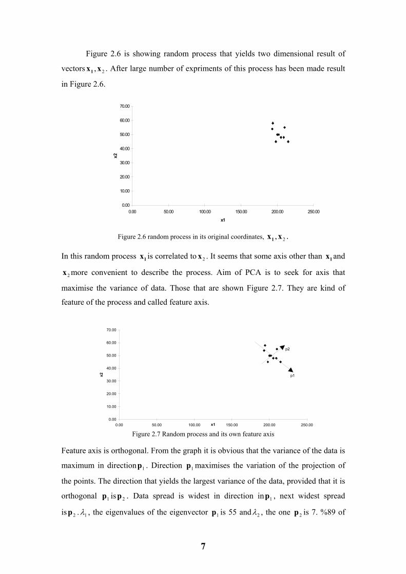
Figure 2.6 is showing random process that yields two dimensional result of

vectors . After large number of expriments of this process has been made result

in Figure 2.6.

2,1 xx

0.00

10.00

20.00

30.00

40.00

50.00

60.00

70.00

0.00 50.00 100.00 150.00 200.00 250.00

x1

x2

Figure 2.6 random process in its original coordinates, . 2,xx1

In this random process is correlated to . It seems that some axis other than x and

more convenient to describe the process. Aim of PCA is to seek for axis that

maximise the variance of data. Those that are shown Figure 2.7. They are kind of

feature of the process and called feature axis.

1x 2x 1

2x

0.00

10.00

20.00

30.00

40.00

50.00

60.00

70.00

0.00 50.00 100.00 150.00 200.00 250.00x1

x2 p1

p2

Figure 2.7 Random process and its own feature axis

Feature axis is orthogonal. From the graph it is obvious that the variance of the data is

maximum in direction . Direction maximises the variation of the projection of

the points. The direction that yields the largest variance of the data, provided that it is

orthogonal isp . Data spread is widest in direction in , next widest spread

is . , the eigenvalues of the eigenvector is 55 and , the one p is 7. %89 of

1p 1p

1p 2 1p

2p 1λ 1p 2λ 2

7

data variance explained by the first feature p and only %11 explained by the second

featurep . This means that p capture most of the variation in original two

dimensional spaces. Least important might be suppressed. Since this reduction of

the dimension suppresses information, it should only be made if the information is not

relevant for next stage of the process. Rotating the original axis by 20 degree in

Figure 2.7.

1

2 1

2p

Figure 2.8. Rotating the original axis by 20 degree.

In Figure 2.8 on the right, the random data in the feature space composed of the two

features. On the left data are represented in a space described only by the first feature

Figure 2.8

Another property of the first principle component,p , is that minimizes the

sum of the squared distance of the observations from their perpendicular projection

onto largest principle component. Variation of the points in the direction of the second

componentp , is smaller than the variation of points in the direction of the largest

principle component .

1

2

1p

8

2.2 Initialization Operations in Face Recognition

The initialization operations in face recognition can be summarized in the following

steps:

1. Acquire an initial set of images (the training set).

2. Calculate the eigenfaces from training set, keeping only the M images correspond to the highest eigenvalues. These eigenfaces define the face space, as new faces are experienced, the eigenfaces can be updated or calculated.

3. Calculate the corresponding distribution in M- dimensional weight space for each known individual, by projecting their face images on to the ‘face space’.

Having initialized system, the following steps are then used to recognize new face

images.

1. Calculate set of weights based on the input image and the M eigenfaces by projecting the input image onto each of the eigenfaces.

2. Determine if the image face at all (whether known or unknown) by checking to see if the image is sufficiently close to “face space”.

3. If it is face, classify the weight pattern as either a known or unknown person.

4. Update the eigenface and/or weight patterns.

5. If the same unknown face is seen several times, calculate characteristic weight pattern and incorporate into known faces.

2.3 Calculating Eigenfaces:

Letting face image I(x,y) two dimentional N by N array of intensity values. Or

vector of dimension if typicall image of size 256x256 becomes vector of

dimension 65,536 or equvalently point in 65,536 dimensional in space. So image then

maps to collection of points in this huge space.

2

2

N

Images of faces being similar in over all configurations will not randomly

distributed in this huge image space and thus can be described by relatively low

dimantional subspace. The main idea of principle component analysis to find

eigevectors that best account for the distributoin of face images within the entire

image space. These vectors define the subspace of face images. Which we call “face

space” each vector of the lenght of . describe NxN image, and linear combination N

9

of original face images. Because these vectors are eigenvectors of covariance matrix

corresponding to the original face images, and because they are face-like appearance,

we refer to them as “eigenfaces” some examples of eigenfaces are shown Figure 2.4.

If the training se of images be . The average face of the set is

defined as:

MΓΓΓ …21 ,

∑=

=M

iiM 1

1 ΓΨ (2.1)

Each face differs from the average face (vector) by the vector (2.2)

ΨΓΦ −= ii (2.2)

Figure 2.9. (a) Face images used as the trainig set (b) The average faceΨ

An example training set is shown in Figure 2.9(a) and average face in Figure 2.9(b). A

set of large vectors is subject to principle component analysis wich seek M

orthonormal vector u which best describes the distribution of the data. The kth vector

, is chosen such that:

k

ku

10

(2

1

1 ∑=

=M

nn

Tkk MΦuλ ) (2.3)

The vectors and λ are the eigenvectors and eigenvalues, respectively, of the

covariance matrix.

ku k

T

Ti

M

iiM

AA

ΦΦC

=

= ∑=

11 (2.4)

Where the marix .The matrix C, however, is by

eigenvector and igenvalues is an intractable task for typical image sizes. We need

a computationally feasible method to find these eigenvectors.

[ M21 ΦΦ,ΦA …= ]2

2 2

T

T=

u

2N

N

If the number of data points in the image space is less han the dimention of

space (M< ), there will be only M, rather , meaningfull eigenvectors.(the

remaining eigenvectors will have eigenvalues of zeros.)

N N

We can solve for dimensional eigenvectors in this case by first solving for

the eigenvectors of MxM matrix. 16x16 matrix rather than 16384x16384 matrix. Then

taking appropriate linear combinations of the face images Φ consider eigenvectors of

such that

2N

i

AA

(2.5) iiiT vAvA µ=

Premultiplying both side by A, we have

(2.6) iiiT AvAvAA µ=

From which we see that are the eigenvectors of (2.4). iAv

Following this analysis we consruct the MxM matrix

where , and find M eigenvectors, of L.These vectors determine linear

combinations of the M training set face images to form the eigenfaces .

AAL T=

,nmmnL φφ lv

l

11

u l (2.7) ∑=

=M

kklkl

1,φv M…1=

With this analyis calculations are greatly reduced, from the order of the number of

pixels in the images( ) to order of the number odf images in the training set

(M< ), and calculation become quite manageable. The associaitive eigenvalues

allow us to rank the eigenvectors according to their usefullness in characterizing the

variation among the images.

2

2

)

ε

N

N

2.4 Using the Eigenfaces Classify a Face Image

Eigenfaces images calculated from the the eigenvectors of L span basis set

with which to describe face images.(Kirby 1987) used M = 115 images an found that

about 40 eigenfaces were sufficint for a very good describtion of the set of face

images. With M = 40 eigenfaces, RMS pixel by pixel errors in representing cropped

version were about %2.

A new face image ( ) is transformed into its eigenfaces components

(projected into “face space”) by a simple operation.

Γ

(2.8) ( ) Mkw Tkk ,,2,1 …=−= ΨΓu

This describes set of point by point image multiplications and summations. Figure

2.10 shows images and their projections onto eigenface space.

Weights form a vector that describes the contribution of

each eigenface in representing the input face image, treating the eigenface as a basis

set for face images.The vector then may then be used in standard pattern recognition

to find which of a number of predifined face classes, if any, best describes the face.

The simplest method for determining which face class provides the best describtion of

an input classΩ that minimize the Euclidian distance of

( MT www …,, 21=Ω

k k

kk Ω−Ω=ε (2.9)

whereΩ is vector describing the kth face class. k

12

A face is classified as belonging to class k when the minimum is below some

chosen threshold , hat defines maximum allowable distance from face space.

Otherwise the face is classified as “unknown” and optionally used to create a new

class.

kε

εθ

'M

2.5 Using Eigenfaces to Detect Faces

By using knowledge of the face space we can recognize the presence of faces.

We can detect and locate faces in single image.

Because creating vector of weights is equvalent to projecting the original the

original face image onto low dimensional space, many image (most of them loooking

nothing like face) will project on to given pattern vector.This not problem for the

system, however since the distance between the image and the face space is simply

the squared distance between mean and input image φ and

,its projection on to face space:

ΨΓ −= ∑=

=1i

iif uwφ

fφφ −=2ε (2.10) 2

Figure 2.10. Three images and their projections onto the face space

defined by the eigenfaces of Figure2.4.

13

From Figure 2.10, images of the faces not change when projected into face space,

while projections of non face images appear quite different. This basic idea is used to

detect the presence of faces in scene; at every location in the image calculate the

distance epsilon between the local sub images and face space. This distance from face

space is used as a measure of a “face ness” So resulting calculating the distance from

face space at every point in the image is a “face map” Figure 2.11. shows

image and image map. Low values (the dark area) indicate presence of a face.

Minimum small dark place in face map correspond location of the face in the image.

Figure 2.11.

),( yxε

Figure 2.11. (a) Original image.(b) Face map,

where low value (dark area) indicate presence of face.

2.6 Face Space Revisited

Faces in the training set, should lie near the face space, which describe images that are

“face like”. Projection distance should be within some threshold .i.e. . There

are four possibilities for an input image and the pattern vector:

εθ θε < εk

1- Near face space near known class.

2- Near face space but not near known class.

3- Distant from face space and near face class.

4- Distant from face space and not near a known face class. Figure 2.12. shows four options for the simple example of two eigenfaces.

In the first case an individual is recognized. In the second case, an unknown

individual is present. Last two cases image is not a face image. Case three shows false

positive. Due to significant distance between image and subspace of shown face.

Figure 3 shows images and their projecting into face space. Figure 2.10 (a) and (b) are

examples of case 1, while Figure 2.10 (c) shows case 4.

14

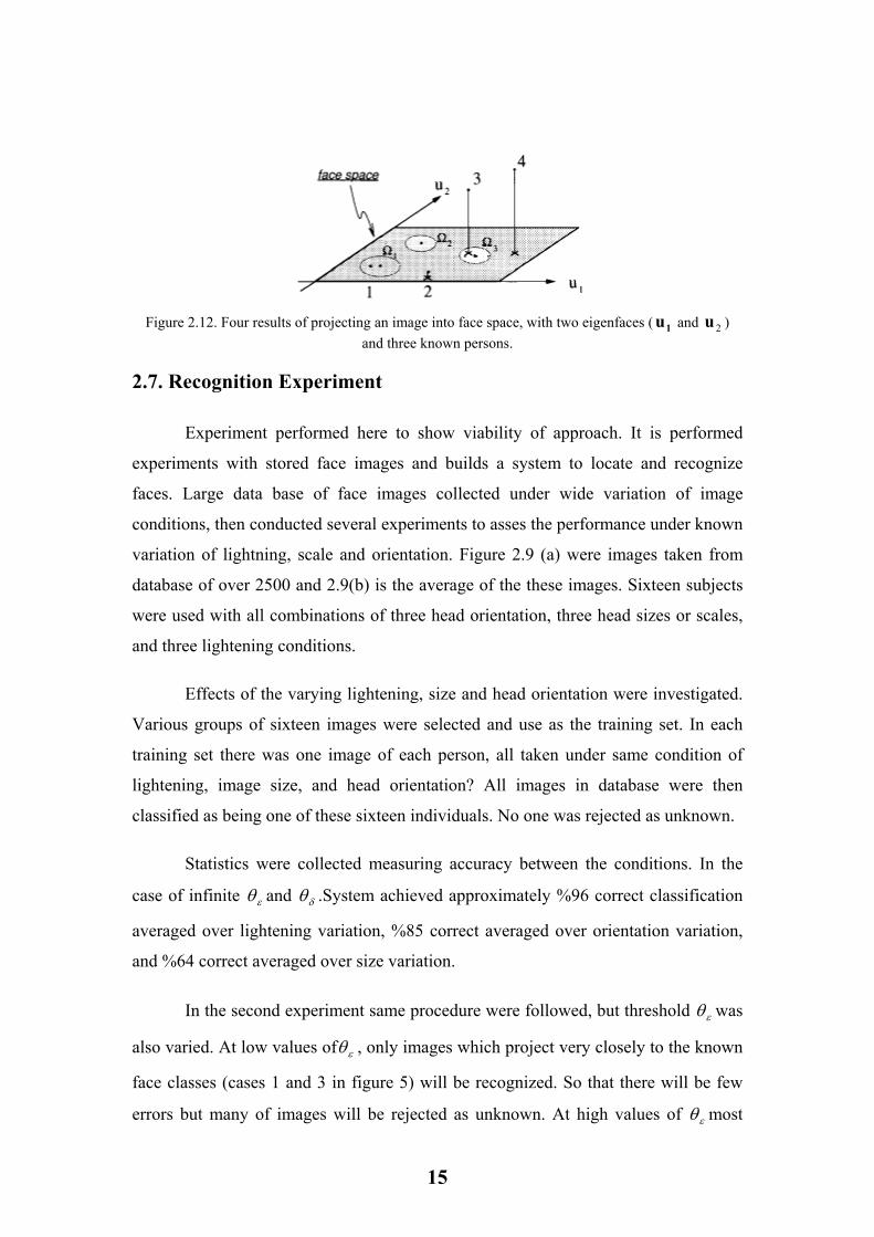
Figure 2.12. Four results of projecting an image into face space, with two eigenfaces ( u and ) 1 2u

and three known persons.

2.7. Recognition Experiment

Experiment performed here to show viability of approach. It is performed

experiments with stored face images and builds a system to locate and recognize

faces. Large data base of face images collected under wide variation of image

conditions, then conducted several experiments to asses the performance under known

variation of lightning, scale and orientation. Figure 2.9 (a) were images taken from

database of over 2500 and 2.9(b) is the average of the these images. Sixteen subjects

were used with all combinations of three head orientation, three head sizes or scales,

and three lightening conditions.

Effects of the varying lightening, size and head orientation were investigated.

Various groups of sixteen images were selected and use as the training set. In each

training set there was one image of each person, all taken under same condition of

lightening, image size, and head orientation? All images in database were then

classified as being one of these sixteen individuals. No one was rejected as unknown.

Statistics were collected measuring accuracy between the conditions. In the

case of infinite and .System achieved approximately %96 correct classification

averaged over lightening variation, %85 correct averaged over orientation variation,

and %64 correct averaged over size variation.

εθ θ

θ

δ

In the second experiment same procedure were followed, but threshold was

also varied. At low values of , only images which project very closely to the known

face classes (cases 1 and 3 in figure 5) will be recognized. So that there will be few

errors but many of images will be rejected as unknown. At high values of most

εθ

εθ

ε

15

images will be classified, but there will be more errors. Adjusting to achieve %100

accurate recognition putting the unknown rates to %19 varying lightening, %39

orientation, and %60 for size. Setting unknown rate arbitrary resulted in correct

recognition rates of %100, %94,%74 respectively.

εθ

Experiments show an increase performance accuracy as the threshold

decreases, which mean that we can catch perfect recognition when threshold goes to

zero. But most of the images rejected as unknown. Also changing lightening

conditions causes errors, but performance drops with in the size change this due to

under lightening changes alone the neighbourhood pixel correlation remains high, but

under size changes the correlation from one image to another is quite low, so there is a

need for a multiscale approach, then faces at particular size are compared with one

another.

Image Processing & Face Extraction

Face Image

Snapshot

Projection into Eigenface Space

Projection Vector

Compare with Projection Vectors of

Training Faces

Not a Face Image

N

Y Near Eigenface

Space

Person ID & Facing Angle Classification

Figure 2.13. Algorithm of Face Recognition.

16

17

CHAPTER 3

RESULTS The algorithm is implemented over a training set of size 18 images. Each

image is in grey level, and has dimensions of 64x64. There are three subjects in the

training set, one man and two women. Each subject gives 6 images, with frontal view

with different gesture and face orientation. Figure 3.1. shows samples in training set.

The training set is found from internet.

(a)

(b)

18

(c)

Figure 3.1. Training Set

The eigenface algorithm firstly forms overall average image. This is the image

just adding all images and dividing by number of images in training set. And the

eigenvectors of covariance matrix that is formed by combining all deviations of

training set’s images from average image is formed in order to apply eigenfaces

algorithm. The average image of the training set is shown in Figure 3.2.

Figure 3.2. Average Image of Training Set

19

After finding overall average image, the order is to find eigenvectors of the

covariance matrix. Since there are 18 images in the training set, we need to find 18

eigenvectors that are used to represent our training set. Visualization of eigenvectors

is carried out simply applying a quantization that is if the found eigenvectors have

components that are greater than 255 and smaller than 0 round them to 255, and 0

respectively. Result of eigenvectors or simply eigenfaces is shown in Figure 3.3 with

corresponding eigenvalues.

20

Figure 3.3. Corresponding Eigenfaces of the training set, with the order of

increasing in eigenvalues.

21

CHAPTER 4

CONCLUSION

System is extended to multi dimensional space; deal with a range of aspects

(other than full frontal views) by defining small number of face classes for each

known person corresponding to characteristics views. Reasoning about images in face

space provides a means to learn and recognize new faces in ‘an unsupervised manner.

When an image very close to face space but it is not classified as one of the familiar

faces, it is labelled as “unknown”. Computer stores pattern vector and corresponding

unknown image. If a collection of “unknown” pattern vectors cluster in the pattern

space, the presence of a new but undefined face is postulated. A noisy image and

partially occluded face should cause recognition performance degrade gracefully.

Since the system implement auto associative memory for known faces. This

evidenced by the projection of the occluded face image, Figure 3.b.

Eigenface approach base on information theory, recognition base on small set

of image features that best approximate the set of known face image, not depends on

intuitive notation of facial part and features. Although it is not first class, it is well

fitted for face recognition, fast simple, work well in constrained environment.

22

REFERENCES

[1].

[2].

[3].

[4].

[5].

W.W. Bledsoe, ”The model method in facial recognition.”, Panoramic

Research Inc. , Palo Alto, CA, Rep. PRI: 15, Aug. 1966.

T. Kanade, “ Picture processing system by computer complex and recognition

of human faces.”, Dept. of Information Science, Kyoto University, Nov. 1973.

P. Burt, “Smart sensing with a pyramidal vision machine,”, Proc. IEEE, Vol.

76, No. 8, Aug. 1988.

T. Kohonen and P. Lehtio,” Storage and processing of information in

distributed associative memory systems,” in G. E. Hinton and J. A. Anderson,

Parallel Models of Associative Memory.

Matthew A. Turk and Allex P. Pentland ,”Face Recognition Using

Eigenfaces”.

23

APPENDIX

MATLAB Source Code

%Implementation of Eigenfaces algorithm %by Sezin KAYMAK %open files orderly clear all M = zeros(64,64); for(i = 1:18) f1 = fopen(num2str(i),'rb'); fread(f1,13,'char'); im = fread(f1,64*64,'uint8'); for(k=1:64) for(m = 1:64) NIM(i,k,m) = im((k-1)*64+m); end end %M = M + NIM; %image(NIM); %colormap('gray'); %pause fclose(f1); end % show 18 figures, each subject in a single figure figure hold for( i = 1 :6) for(k = 1:64) for(l =1:64) x(k,l)=NIM(i,k,l); end end subplot(3,2,i),image(x); end colormap('gray'); figure hold for( i = 7 :12) for(k = 1:64) for(l =1:64) x(k,l)=NIM(i,k,l); end end subplot(3,2,i-6),image(x); end colormap('gray'); figure

24

hold for( i = 13 :18) for(k = 1:64) for(l =1:64) x(k,l)=NIM(i,k,l); end end subplot(3,2,i-12),image(x); end colormap('gray'); data = double(NIM); %M = M/18; %image(M); %colormap('gray'); %average vector G = zeros(64*64,18); for(i = 1:18) for(j = 1:64) for(k = 1:64) G((j-1)*64+k,i)=data(i,j,k); end end end Y = zeros(64*64,1); for(i = 1:18) for(j = 1:(64*64)) Y(j,1) = Y(j,1)+G(j,i); end end Y = Y / 18; %end of average finding %show average image for(k = 1:64) for(l = 1:64) x(k,l) = Y((k-1)*64+l); end end figure image(uint8(x)); colormap('gray'); pause; % form A for( i = 1:18) A(:,i) = G(:,i)-Y; end

25

%find L L = A'*A; %find eigenvalue and eigenvector [V,lamda] = eig(L); %find eigenfaces u = zeros(64*64,18); for(i = 1:18) for(j = 1:18) u(:,i) = u(:,i)+V(i,j)*A(:,j); end end % check eigenfaces for(i = 1:18) for(j = 1:64) for(k = 1:64) EigenFaces(j,k,i)=round(u((j-1)*64+k,i)); if(EigenFaces(j,k,i)<0) EigenFaces(j,k,i) = 0; end if(EigenFaces(j,k,i)>255) EigenFaces(j,k,i) = 255; end end end end %plot eigenfaces figure for(i = 1:6) subplot(3,2,i),image(EigenFaces(:,:,i)); xlabel(['Eigen Value = ' num2str(lamda(i,i))]); colormap('gray'); pause end figure for(i = 7:12) subplot(3,2,i-6),image(EigenFaces(:,:,i)); xlabel(['Eigen Value = ' num2str(lamda(i,i))]); colormap('gray'); pause end figure for(i = 13:18) subplot(3,2,i-12),image(EigenFaces(:,:,i));

26

xlabel(['Eigen Value = ' num2str(lamda(i,i))]); colormap('gray'); pause end % calculat weght w=zeros (18,18); for (i=1:18) for(j=1:18) w(i,j)=u(:,j)'*(G(:,i)-Y); end end

27