Embed Size (px)
Citation preview

Face Detection and Recognition inVideo-Streams
Jannik Boll Nielsen
Kongens Lyngby 2010IMM-B.Sc-2010-14

Technical University of DenmarkInformatics and Mathematical ModellingBuilding 321, DK-2800 Kongens Lyngby, DenmarkPhone +45 45253351, Fax +45 [email protected]
IMM-B.Sc: ISSN 0909-3192

Abstract
Using the Viola Jones face detection algorithm and Active Appearance Models,it is shown that high success rate face-recognition in video-streams is possiblewith a relatively low processing time.Limitations in the Active Appearance Model Software by Stegmann et al. [15]forced us discard the original thought of doing a recognition based on parame-ters from a match, using a general model of the human face. Instead we decidedto build an Active Appearance Model representing the subject being searchedfor, and use this model to do a recognition based on statistical thresholds ofdeviance.Tests have proven very high success rates. Detection rate of faces in the video-footage reached 98,38% with only 1,60% erroneous detections, recognition ratesper frame reached 66,67% with 0% erroneous and finally the overall sequencerecognitions proved a rate of 88,90% while maintaining 0% erroneous recogni-tions.The test results clearly indicates that Active Appearance Models are capable ofdoing high quality face recognitions. Extending the software in order to searchfor more than one face can easily be done, the computing time however will bedoubled whenever the number of Active Appearance Models are being doubled.Had it been possible to do the parameter based recognition, the computingtime of the recognition would have remained the same, however recognition ofmultiple faces would not have any noticeable effect on the computing time.

ii

Preface
Both the Viola Jones face detection algorithm and Active Appearance Modelshave over the last years proven as very robust tools in the domain of imageanalysis. The speed of the Viola Jones algorithm as well as the flexibility of theActive Appearance Models has already found way to into modern technologiesin form of face-detecting cameras and intelligent medical equipment able torecognize elements in the human body. Based on this, the idea of detecting andrecognizing human faces using such methods seems very appealing and not aschallenging as it has been in the past, using older methods of recognition anddetection.Using the OpenCV C-programming package [6] face-detection will be performedwith the Viola Jones algorithm. Recognition of the detected faces will then beperformed using the Active Appearance Model software by Stegmann et al. [15].Since I am studying Electrical Engineering, I have chosen to write all code in theC programming language in order to emphasize, that such software can easilybe implemented in a hardware solution. This makes the project very relevantfor electrical engineers as well.I would like to thank my supervisor, Professor Rasmus Larsen, for doing a greatjob in supervising this project of mine. Also I would like to thank AssociateProfessor Rasmus Reinhold Paulsen, Assistant Professor Line Katrine HarderClemmensen and PostDoc Anders Lindbjerg Dahl for their weekly supervisionwhich has also been invaluable and beyond any expectations.

iv

Contents
Abstract i
1 Introduction 11.1 Background . . . . . . . . . . . . . . . . . . . . . . . . . . . . . . 11.2 Existing Face Detection Methods . . . . . . . . . . . . . . . . . . 21.3 Existing Face Recognition Methods . . . . . . . . . . . . . . . . . 31.4 Problem Statement . . . . . . . . . . . . . . . . . . . . . . . . . . 41.5 Delimitation . . . . . . . . . . . . . . . . . . . . . . . . . . . . . . 4
2 Theory 72.1 The Viola Jones Detector . . . . . . . . . . . . . . . . . . . . . . 72.2 Continuity Filtering . . . . . . . . . . . . . . . . . . . . . . . . . 112.3 The Active Appearance Model . . . . . . . . . . . . . . . . . . . 142.4 The Active Appearance Model Search . . . . . . . . . . . . . . . 182.5 Recognition using Active Appearance Models . . . . . . . . . . . 202.6 The Active Appearance Model Threshold . . . . . . . . . . . . . 212.7 OpenCV . . . . . . . . . . . . . . . . . . . . . . . . . . . . . . . . 23
3 Implementation 253.1 Limitations of the Active Appearance Model software . . . . . . 253.2 Snapshotting Faces . . . . . . . . . . . . . . . . . . . . . . . . . . 263.3 Building an Active Appearance Model . . . . . . . . . . . . . . . 283.4 Recognition using Active Appearance Models . . . . . . . . . . . 28
4 Results and Discussion 314.1 Detection Results . . . . . . . . . . . . . . . . . . . . . . . . . . . 314.2 Recognition Results . . . . . . . . . . . . . . . . . . . . . . . . . 324.3 Discussion . . . . . . . . . . . . . . . . . . . . . . . . . . . . . . . 33

vi CONTENTS
5 Conclusion 375.1 Conclusion . . . . . . . . . . . . . . . . . . . . . . . . . . . . . . 375.2 Future Work . . . . . . . . . . . . . . . . . . . . . . . . . . . . . 37
A Test Data 39
B AAM Training-set 45
C Software Manual 47C.1 Calling the Software . . . . . . . . . . . . . . . . . . . . . . . . . 47C.2 Changing the Settings . . . . . . . . . . . . . . . . . . . . . . . . 48C.3 Reading the Output . . . . . . . . . . . . . . . . . . . . . . . . . 48C.4 Known bugs . . . . . . . . . . . . . . . . . . . . . . . . . . . . . . 48

List of Figures
1.1 Cameras with face-detectors . . . . . . . . . . . . . . . . . . . . . 2
2.1 The Integral Image . . . . . . . . . . . . . . . . . . . . . . . . . . 8
2.2 Using an Integral Image . . . . . . . . . . . . . . . . . . . . . . . 8
2.3 Common features . . . . . . . . . . . . . . . . . . . . . . . . . . . 9
2.4 Common features . . . . . . . . . . . . . . . . . . . . . . . . . . . 9
2.5 Frontal face . . . . . . . . . . . . . . . . . . . . . . . . . . . . . . 11
2.6 Common features generated from frontal faces . . . . . . . . . . . 11
2.7 Erroneous Detections . . . . . . . . . . . . . . . . . . . . . . . . . 12
2.8 Continuity Filter Flow-table . . . . . . . . . . . . . . . . . . . . . 14
2.9 Errors after filtering . . . . . . . . . . . . . . . . . . . . . . . . . 15
2.10 Geometrical facial features . . . . . . . . . . . . . . . . . . . . . . 16
2.11 AAM Search . . . . . . . . . . . . . . . . . . . . . . . . . . . . . 20
2.12 The χ2 distribution . . . . . . . . . . . . . . . . . . . . . . . . . . 22

viii LIST OF FIGURES
3.1 Snapshot scaling and translation . . . . . . . . . . . . . . . . . . 27
3.2 Variations in an AAM . . . . . . . . . . . . . . . . . . . . . . . . 30
4.1 Face Detection Results . . . . . . . . . . . . . . . . . . . . . . . . 32
4.2 ROC Curve of Face Detections . . . . . . . . . . . . . . . . . . . 33
4.3 Face Recognition Results per frame . . . . . . . . . . . . . . . . . 34
4.4 Face Recognition Results per sequence . . . . . . . . . . . . . . . 35
4.5 ROC Curve of Face Recognitions . . . . . . . . . . . . . . . . . . 35
B.1 Training images for AAM . . . . . . . . . . . . . . . . . . . . . . 46

List of Tables
A.1 Viola Jones Detections 1 . . . . . . . . . . . . . . . . . . . . . . . 39
A.2 Viola Jones Detections 2 . . . . . . . . . . . . . . . . . . . . . . . 40
A.3 Viola Jones Detections 3 . . . . . . . . . . . . . . . . . . . . . . . 40
A.4 Viola Jones Detections 4 . . . . . . . . . . . . . . . . . . . . . . . 40
A.5 Recognition per frame 1 . . . . . . . . . . . . . . . . . . . . . . . 41
A.6 Recognition per frame 2 . . . . . . . . . . . . . . . . . . . . . . . 41
A.7 Recognition per frame 3 . . . . . . . . . . . . . . . . . . . . . . . 42
A.8 Recognition per video 1 . . . . . . . . . . . . . . . . . . . . . . . 42
A.9 Recognition per video 2 . . . . . . . . . . . . . . . . . . . . . . . 43
A.10 Recognition per video 3 . . . . . . . . . . . . . . . . . . . . . . . 43
A.11 Recognition per video 4 . . . . . . . . . . . . . . . . . . . . . . . 44

x LIST OF TABLES

Chapter 1
Introduction
1.1 Background
A lot of video footage exists in archives, much of this includes people. Thefootage is however not always properly documented and does therefore oftennot contain proper information about which people have been filmed. As thecontents of video archives is ever increasing, it is needed to find ways of annotat-ing relevant people included in the many footages. To speed up this extensiveprocess, facial recognition and matching, could be applied, using modern com-puters.In some cases only one, or a short list of people are needed to be recognized, forexample when looking for a certain actor or politician. Here, the issue is notwho is there, but rather if a certain person is there. A "White List" contain-ing the faces of the requested people could be matched with the faces found invideo archives, in order to decide if any of these faces are present and if so, whoappears where.
2 Introduction
1.2 Existing Face Detection Methods
Among the algorithms for detecting faces within an image, 3 important onesare the Viola-Jones Object Detection Framework [19], the Schneiderman andKanade Statistical Detection Approach [11] and the Neural Network-BasedFace Detection [4]. These methods all have a high efficiency rate in detectingfaces, but only the Viola Jones algorithm has proven fast enough for real-timedetections[7].Schneiderman and Kanade uses an approach where a product of histogramsfrom subsections of an image, are used in order to statistically determine iffaces are present. Using multiple statistical templates, multiple orientations offaces can be detected, making the detector more robust. Unfortunately this de-tector suffers from the low processing speed and is therefore hard to implementin real-time applications.The Neural Network based detector uses a set of neural networks trained fordetermining the presence or absence of faces based on pixel intensities. The ma-jor disadvantage of this detector, is that the neural networks must learn whatis not a face, which is very hard to teach considering how many pixel-intensitycombinations are not a face, compared to the number of combinations that are.Furthermore also the speed of this detector is not high enough for real-timeapplications.The Viola Jones detector has the advantage, compared to the Neural Networkbased, that it does not need to know what is not a face. It only needs to knowwhat can be a face. The speed of this detector, is the only of the 3 mentionedthat actually allows for real-time detection. This detector will be explainedin-depth later in this paper.
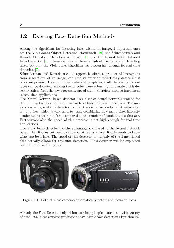
Figure 1.1: Both of these cameras automatically detect and focus on faces.
Already the Face Detection algorithms are being implemented in a wide varietyof products. Most cameras produced today, have a face detection algorithm im-
1.3 Existing Face Recognition Methods 3
plemented to assure proper focus. Recently, also cameras using a smile detectorhave been presented, assuring happy faces in pictures. In figure 1.1 two camerasfrom Canon and Sony respectively are shown, both of these cameras use facedetection algorithms to detect faces and focus on these.
1.3 Existing Face Recognition Methods
So far, multiple methods of recognizing faces have been developed, some moresuccessful than others.Among the traditional methods are the geometric and photometric approaches.The geometric approach measures the face’s geometric features, such as eye-width/distance, jaw-size and so forth, while the photometric approach is a viewbased approach, that extracts a line of statistical, photometric features and eval-uates those [16].Among the methods developed, the most studied are the PCA (Principal Com-ponents Analysis, or Eigenface method), the LDA (Linear Discriminant Analy-sis) and the EBGM (Elastic Bunch Graph Matching) [16].Recently new approaches to the face recognition problem has appeared. Thesenew approaches involve 3D facial recognition, using 3D models of faces gener-ated by for example stereo-cameras[9], and recognition based on skin textureanalysis.The 3D model approach can achieve very high recognition rates reaching up to97% success and close to 0% erroneous recognition [5]. The major drawback ofthis type of recognition is the amount of preparation needed in order to do amatch: The face must be recorded in 3D, which is not always possible dependingon the application. If one is able to control the recognition environment e.g. alogin-facility, this method is definitely a possibility, however if recognition is tobe performed on random images, the usage is limited.The method of recognising using Eigenfaces is based on projecting a face into asubspace spanned by trained Eigenfaces. Based on the subspace-position of theface and a priori knowledge of the subspace-position of the faces being searchedfor, a statistical evaluation can be performed in order to classify or reject theface as a match [18]. This method has also proven successful with correct recog-nitions of close to 100%, although unable to classify roughly 40% of the the facespresented [18].
The companies Google and Apple have both lately presented new image or-ganizer software1 for private use, that enables users to build and search photo-collections based on face recognition. The company L-1 specializes in recognition
1Google Picasa and Apple IPhoto

4 Introduction
systems including face-recognition-based. This company is one of the leadingcompanies in the world when it comes to face-recognition and presents a lot ofsolutions enabling customers to recognize faces. Some applications even providereal-time recognition [13].
1.4 Problem Statement
This project involves two key subjects.
• Use the Viola Jones algorithm through relevant C-programming packages(OpenCV) and thereby extract faces from a number of given video record-ings.
• Use Active Appearance Models software (either API or Standalone) to tryand match the faces found, via. the Viola Jones algorithm, with up to 10images contained in a "White List" in order to decide, whether or not one,or more, of these "White Listed" people appears in the video footage.
While using the Viola Jones face-detector, it is important to be able to distin-guish the faces, to a certain degree, in order to decide if the face found is in factthe same as the one in previous frame (but moved slightly), or if it is actuallya new face. Without this filtering, an overflow of duplicates would probablyappear.
Since the face-detection is done on multiple frames, one could expect that a"high quality Viola Jones match" would be found at some point. If this is thecase, a very high success-threshold could be used, which would likely make thefinal AAM-White-List-matching easier.
1.5 Delimitation
The Viola Jones algorithm uses a trained classifier cascade in order to detectfaces. Training such a cascade is beyond the scope of the project and is in fact arather extensive project in itself. One must therefore rely on finding an alreadytrained cascade. Cascades are available on many websites on the internet, oneexample is [12] which provides multiple cascades including frontal face, profileand head + shoulders.

1.5 Delimitation 5
Also building a very general Active Appearance Model is a rather time con-suming process, requiring a very large collection of annotated faces containinglarge variation in appearance. Due to this fact, one must find a compromisebetween the quality of the Appearance Model and the time spent training it.
Finally, since this is a "proof of concept", little weight is put on the qualityof the code and is not considered important for the purpose of this paper.

6 Introduction
Chapter 2
Theory
In this chapter relevant theory concerning the Viola Jones Face Detector andActive Appearance Models will be explained. Initially the Viola Jones Detectoralgorithm, as well as its cascade of classifiers, will be presented. Subsequentlyan approach to filter out erroneous detections based on time-space constraintswill be presented in the section Continuity Filtering. This theory is the basis ofall face detection executed in the recognition software.Afterwards, a theoretical explanation of the Active Appearance Models, includ-ing the search and the goodness of fit estimation, is presented. Where theprevious sections explains the concepts of detecting faces, these sections con-cerns theory of recognizing faces from the detections.Finally a brief introduction to the usage of OpenCV is made.
2.1 The Viola Jones Detector
2.1.1 The Algorithm
The Viola Jones Face Detection Algorithm uses a so-called Integral Image tospeed up the calculation of rectangular features. The Integral Image resembles

8 Theory
"Summed area tables" and is defined as as the sum of all values left of and abovethe current coordinate:
ii(x, y) =N∑
x′≤x,y′≤y
i(x′, y′)
Where ii(x, y) is the integral image and i(x, y) is the original input image.In figure 2.1 this procedure is illustrated on a 3*3 pixels image. This entire
1 1 11 1 11 1 1
1 2 32 4 63 6 9
Figure 2.1: Original Image v.s. Integral Image
integral image can be calculated in a single pass [19].As stated, it is very easy to calculate rectangular sums within the input image,using its integral image. This is illustrated in figure 2.2 where the sum of theshaded rectangle, is easily calculated using the values A, B, C and D from theintegral image. Thus the sum of the shaded rectangle is given by:∑
ShadedRectangle = D − (B + C) +A
Any given sum can therefore be calculated using only 4 references.By using the integral image, one can very easily check for features at arbitrary
Figure 2.2: Calculation of shaded rectangle.
locations within an image, since the calculated sums give a direct indication ofthe color-intensity at a given area.Some common features are presented in figure 2.3 [7]. In these features the
2.1 The Viola Jones Detector 9
Figure 2.3: Common features
required rectangles range from 2 to 4, requiring from 6 to 9 integral image ref-erences.
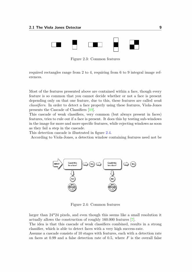
Most of the features presented above are contained within a face, though everyfeature is so common that you cannot decide whether or not a face is presentdepending only on that one feature, due to this, these features are called weakclassifiers. In order to detect a face properly using these features, Viola-Jonespresents the Cascade of Classifiers [19].This cascade of weak classifiers, very common (but always present in faces)features, tries to rule out if a face is present. It does this by testing sub-windowsin the image for more and more specific features, while rejecting windows as soonas they fail a step in the cascade.This detection cascade is illustrated in figure 2.4.According to Viola-Jones, a detection window containing features need not be
Figure 2.4: Common features
larger than 24*24 pixels, and even though this seems like a small resolution itactually allows the construction of roughly 160.000 features [7].The idea is that this cascade of weak classifiers combined, results in a strongclassifier, which is able to detect faces with a very high success-rate.Assume a cascade consists of 10 stages with features, each with a detection rateon faces at 0.99 and a false detection rate of 0.5, where F is the overall false
10 Theory
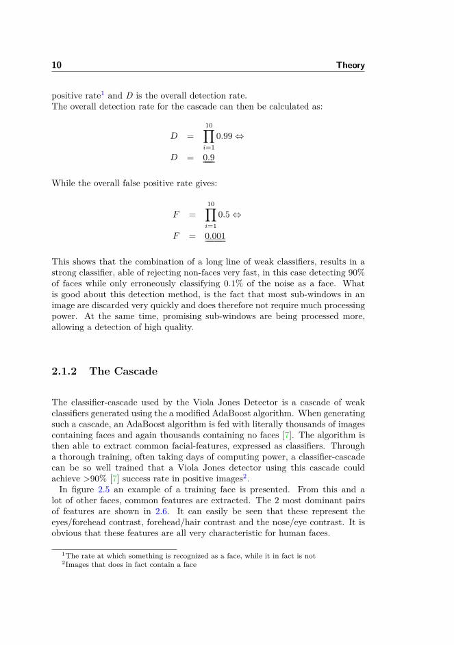
positive rate1 and D is the overall detection rate.The overall detection rate for the cascade can then be calculated as:
D =10∏i=1
0.99⇔
D = 0.9
While the overall false positive rate gives:
F =10∏i=1
0.5⇔
F = 0.001
This shows that the combination of a long line of weak classifiers, results in astrong classifier, able of rejecting non-faces very fast, in this case detecting 90%of faces while only erroneously classifying 0.1% of the noise as a face. Whatis good about this detection method, is the fact that most sub-windows in animage are discarded very quickly and does therefore not require much processingpower. At the same time, promising sub-windows are being processed more,allowing a detection of high quality.
2.1.2 The Cascade
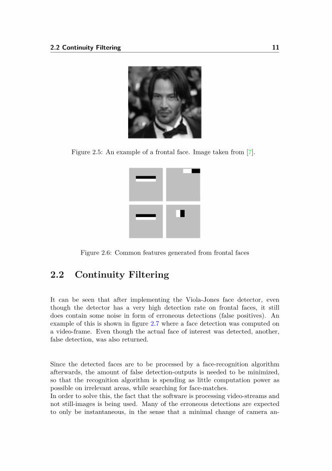
The classifier-cascade used by the Viola Jones Detector is a cascade of weakclassifiers generated using the a modified AdaBoost algorithm. When generatingsuch a cascade, an AdaBoost algorithm is fed with literally thousands of imagescontaining faces and again thousands containing no faces [7]. The algorithm isthen able to extract common facial-features, expressed as classifiers. Througha thorough training, often taking days of computing power, a classifier-cascadecan be so well trained that a Viola Jones detector using this cascade couldachieve >90% [7] success rate in positive images2.In figure 2.5 an example of a training face is presented. From this and a
lot of other faces, common features are extracted. The 2 most dominant pairsof features are shown in 2.6. It can easily be seen that these represent theeyes/forehead contrast, forehead/hair contrast and the nose/eye contrast. It isobvious that these features are all very characteristic for human faces.
1The rate at which something is recognized as a face, while it in fact is not2Images that does in fact contain a face
2.2 Continuity Filtering 11
Figure 2.5: An example of a frontal face. Image taken from [7].
Figure 2.6: Common features generated from frontal faces
2.2 Continuity Filtering
It can be seen that after implementing the Viola-Jones face detector, eventhough the detector has a very high detection rate on frontal faces, it stilldoes contain some noise in form of erroneous detections (false positives). Anexample of this is shown in figure 2.7 where a face detection was computed ona video-frame. Even though the actual face of interest was detected, another,false detection, was also returned.
Since the detected faces are to be processed by a face-recognition algorithmafterwards, the amount of false detection-outputs is needed to be minimized,so that the recognition algorithm is spending as little computation power aspossible on irrelevant areas, while searching for face-matches.In order to solve this, the fact that the software is processing video-streams andnot still-images is being used. Many of the erroneous detections are expectedto only be instantaneous, in the sense that a minimal change of camera an-

12 Theory
Figure 2.7: The Viola-Jones algorithm successfully detects the face of interest,unfortunately it also detects something that is not a face.
gle or lightening condition would obscure the false detection. By searching fortime-dependant continuity in detection positions and -sizes, one is able to filterout the majority of the noise the Viola-Jones algorithm produces in a still-image.
An algorithm was designed, enabling this feature.Pseudo-code is as follows:
1. A 2 dimensional array is created, where the length of the first coordinate isdetermined by the amount of detections allowed to be processed per frameand the length of the second coordinate is determined by the amount offrames a face is allowed to skip, in order to still be classified as "the sameface as before".
2. Start processing first frame as follows:
• Detect all faces. if there are no faces, go back to (2) and process nextframe.
• For each detected face,
– add it to the last column in the array.– If any previous detection in the array has a size and position
within threshold: copy its score, increment it by 1, and assign itto this detection.
2.2 Continuity Filtering 13
• Delete the first column and shift all other columns one left. (i.e.increment the time passed)• Go back to (2) and process next frame.
3. While processing the detections, only current frames within the array con-taining a score above a certain threshold is then marked/saved/furtherprocessed.
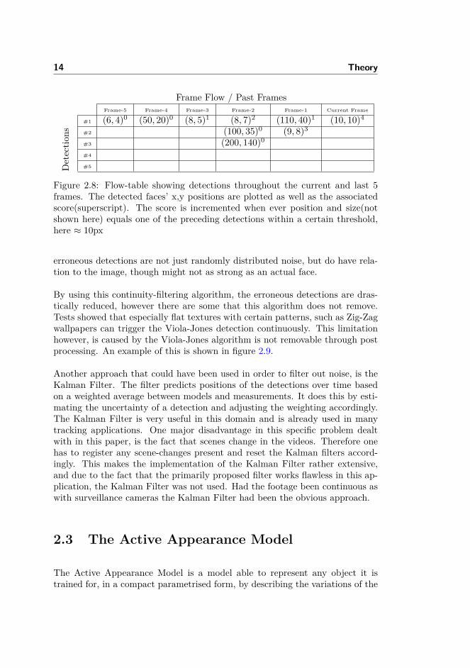
The iteration process is illustrated in figure 2.8 where a detection frame-jumpof maximum 5 frames is allowed. Whenever a face is detected that is in theproximity of one of the detections in the previous 5 frames, the score of this faceis incremented. In this way, the score indicates whether a certain detection hasa high or low probability of actually being a face.
One could do some statistical considerations concerning this method of filtering.Assuming that a face-detector has an erroneous detection rate Perror, one canestimate the probability of the same error appearing multiple times under theassumption that the scene has changed considerably between each sample. If itis assumed that it takes n frames in order for the scene to not be identical to theprevious and the detector registers a face m times in a row, then the numberof uncorrelated detections will be m
n and the total probability of observing thesame error at the same location multiple times, called Ptotal, would be:
Ptotal =mn∏1Perror ⇔ (2.1)
Ptotal = (Perror)mn (2.2)
In the implementation, a score threshold of 15 detections was set. Assuming,rather crudely, that it takes 5 frames for detections to be uncorrelated, oneobtains m
n = 155 = 3. With an erroneous detection rate of Perror = 0.1 from the
detector, the total probability of an error appearing 15 times will be:
Ptotal = (0.1)3 ⇔Ptotal = 0.001
Indicating a 0.1% probability of misclassification. This is however a very crudeapproximation since frames will always be somewhat correlated. Moreover, the
14 Theory
Frame Flow / Past FramesFrame-5 Frame-4 Frame-3 Frame-2 Frame-1 Current Frame
Detectio
ns
#1 (6, 4)0 (50, 20)0 (8, 5)1 (8, 7)2 (110, 40)1 (10, 10)4
#2 (100, 35)0 (9, 8)3
#3 (200, 140)0
#4
#5
Figure 2.8: Flow-table showing detections throughout the current and last 5frames. The detected faces’ x,y positions are plotted as well as the associatedscore(superscript). The score is incremented when ever position and size(notshown here) equals one of the preceding detections within a certain threshold,here ≈ 10px
erroneous detections are not just randomly distributed noise, but do have rela-tion to the image, though might not as strong as an actual face.
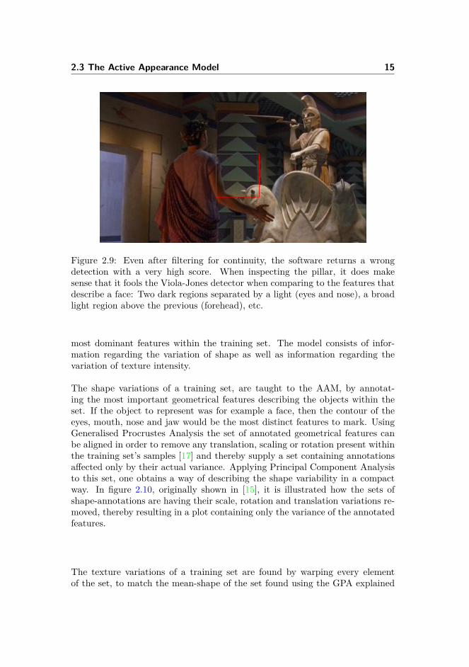
By using this continuity-filtering algorithm, the erroneous detections are dras-tically reduced, however there are some that this algorithm does not remove.Tests showed that especially flat textures with certain patterns, such as Zig-Zagwallpapers can trigger the Viola-Jones detection continuously. This limitationhowever, is caused by the Viola-Jones algorithm is not removable through postprocessing. An example of this is shown in figure 2.9.
Another approach that could have been used in order to filter out noise, is theKalman Filter. The filter predicts positions of the detections over time basedon a weighted average between models and measurements. It does this by esti-mating the uncertainty of a detection and adjusting the weighting accordingly.The Kalman Filter is very useful in this domain and is already used in manytracking applications. One major disadvantage in this specific problem dealtwith in this paper, is the fact that scenes change in the videos. Therefore onehas to register any scene-changes present and reset the Kalman filters accord-ingly. This makes the implementation of the Kalman Filter rather extensive,and due to the fact that the primarily proposed filter works flawless in this ap-plication, the Kalman Filter was not used. Had the footage been continuous aswith surveillance cameras the Kalman Filter had been the obvious approach.
2.3 The Active Appearance Model
The Active Appearance Model is a model able to represent any object it istrained for, in a compact parametrised form, by describing the variations of the
2.3 The Active Appearance Model 15
Figure 2.9: Even after filtering for continuity, the software returns a wrongdetection with a very high score. When inspecting the pillar, it does makesense that it fools the Viola-Jones detector when comparing to the features thatdescribe a face: Two dark regions separated by a light (eyes and nose), a broadlight region above the previous (forehead), etc.
most dominant features within the training set. The model consists of infor-mation regarding the variation of shape as well as information regarding thevariation of texture intensity.
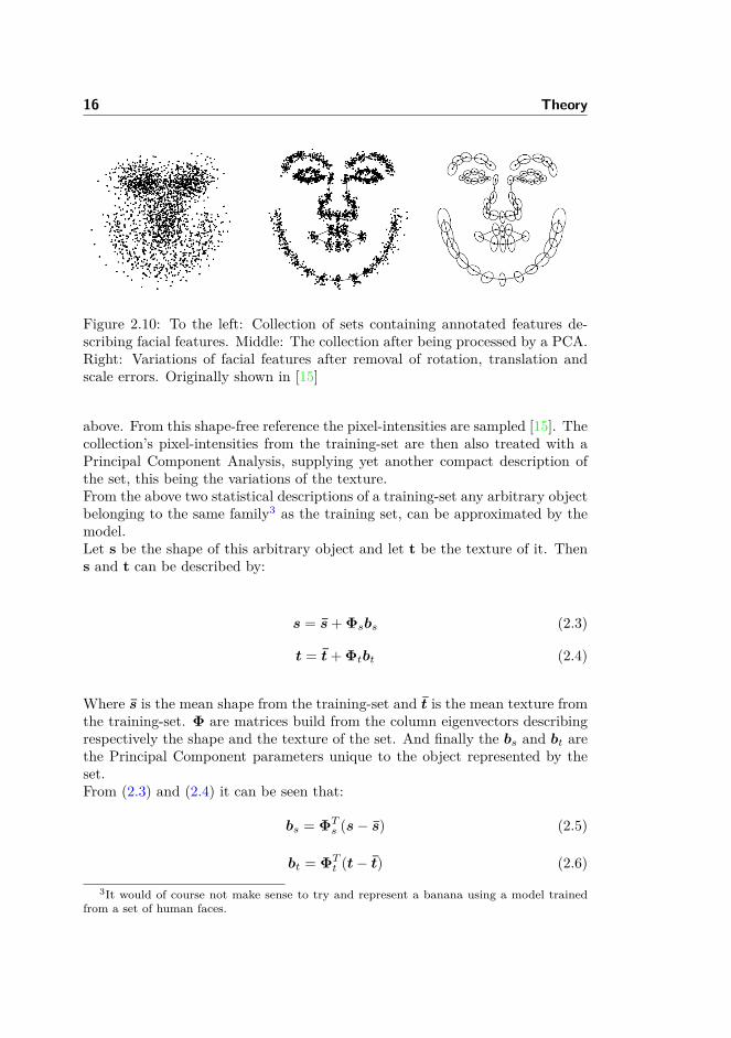
The shape variations of a training set, are taught to the AAM, by annotat-ing the most important geometrical features describing the objects within theset. If the object to represent was for example a face, then the contour of theeyes, mouth, nose and jaw would be the most distinct features to mark. UsingGeneralised Procrustes Analysis the set of annotated geometrical features canbe aligned in order to remove any translation, scaling or rotation present withinthe training set’s samples [17] and thereby supply a set containing annotationsaffected only by their actual variance. Applying Principal Component Analysisto this set, one obtains a way of describing the shape variability in a compactway. In figure 2.10, originally shown in [15], it is illustrated how the sets ofshape-annotations are having their scale, rotation and translation variations re-moved, thereby resulting in a plot containing only the variance of the annotatedfeatures.
The texture variations of a training set are found by warping every elementof the set, to match the mean-shape of the set found using the GPA explained
16 Theory
Figure 2.10: To the left: Collection of sets containing annotated features de-scribing facial features. Middle: The collection after being processed by a PCA.Right: Variations of facial features after removal of rotation, translation andscale errors. Originally shown in [15]
above. From this shape-free reference the pixel-intensities are sampled [15]. Thecollection’s pixel-intensities from the training-set are then also treated with aPrincipal Component Analysis, supplying yet another compact description ofthe set, this being the variations of the texture.From the above two statistical descriptions of a training-set any arbitrary objectbelonging to the same family3 as the training set, can be approximated by themodel.Let s be the shape of this arbitrary object and let t be the texture of it. Thens and t can be described by:
s = s̄+ Φsbs (2.3)
t = t̄+ Φtbt (2.4)
Where s̄ is the mean shape from the training-set and t̄ is the mean texture fromthe training-set. Φ are matrices build from the column eigenvectors describingrespectively the shape and the texture of the set. And finally the bs and bt arethe Principal Component parameters unique to the object represented by theset.From (2.3) and (2.4) it can be seen that:
bs = ΦTs (s− s̄) (2.5)
bt = ΦTt (t− t̄) (2.6)
3It would of course not make sense to try and represent a banana using a model trainedfrom a set of human faces.
2.3 The Active Appearance Model 17
Instead of having two distinct parametrisations (bs and bt), these can be com-bined to form one single vector, c. However in order to obtain this shape-texturecombined parametrisation c, a final PCA must be performed in order to accom-modate for any correlation there might be between shape and pixel-intensities.This is done in the following:
bs and bt are combined into b using a weighting represented by the diagonalmatrix W s.
b =[W sbsbt
]=[W sΦT
s (s− s̄)ΦTt (t− t̄)
](2.7)
Stegmann et al. mentions that the typical weighting is done so the shape Prin-cipal Scores (bs) are weighted by the square root of the ratio between the sumsof the texture and shape eigenvalues [15].
Coupling the shape and texture eigenspaces through the third PCA then re-sults in the combined parameters describing variances in shape and texture aswell as their common correlation:
b = Φcc =[Φc,s
Φc,t
]c (2.8)
With this, (2.7) and (2.8) can be combined, resulting in a statistical descriptionof the arbitrary object being:
s = s̄+ ΦsW−1s Φc,sc (2.9)
t = t̄+ ΦtΦc,tc (2.10)
Where the object is now described using only one set of parameters, describingthe full coupled appearance.What (2.9) and (2.10) tells, is that adjusting only the values of the vector c,one is able to model any given appearance belonging to the same family as thetraining-set.This leads to second aspect of Active Appearance Models: Finding the bestmatch between a model and an underlying image by adjusting the appearanceparameters in c. However, before continuing to this matter, a brief comment onhow to build an Active Appearance Model is now presented.
18 Theory
2.3.1 Building an Active Appearance Model
In order to extract parameters describing shape- and textural-features, an Ac-tive Appearance Model must be built. This model must be trained using a widevariety of faces presenting different lightening conditions, facial expressions andorientations. The model must be as general as possible enabling it to match anyarbitrary pose, expression and texture of an unknown face.
M. B. Stegmann presents in his work FAME - A Flexible Appearance ModellingEnvironment [15] a collection of different annotated faces. With this collectionit is possible to train an Active Appearance Model of the human face, containingparameters describing face-positions, textural- and shape-features and expres-sions, based on the actual variations present within the collection of faces. Thiscan be done Using the console-software also available through [15].
The annotation process is rather time consuming due to the fact that it is donemanually. Edwards et al. therefore suggests doing this annotation semi- or fullyautomated, since the environment of the training faces can be fully controlled[17].
2.4 The Active Appearance Model Search
The Active Appearance Model Search is basically how a model is able to fit itselfto an underlying image, i.e. how to iterate through the model-parameters inorder to obtain the minimum error possible, between model and image. Multipleways of doing this exists, however only one will be explained here: the FixedJacobian Matrix Estimate [17], which is the one used in the AAM software byM. Stegmann and therefore also used in this project [15].In order to solve this optimization, an error-vector r(p) is introduced. Thisvector is an indication of the pixel-intensity-error between the model and thepicture below. r(p) is defined as:
r(p) = timage(p)− tmodel(p) (2.11)
Where timage(p) and tmodel(p) are the texture vectors describing respectivelythe image texture under the model and the model-texture.If p∗ is a set of parameters in the proximity of the optimum parameter-set: p+,the Taylor Expansion of the error is then:

2.4 The Active Appearance Model Search 19
r(p∗ + δp) ≈ r(p∗) + ∂r(p∗)∂p
δp (2.12)
Where the differential component ∂r(p∗)∂p is:
∂r(p∗)∂p
= ∂r
∂p=
∂r1
∂p1· · · ∂r1
∂pQ...
. . ....
∂rM∂p1
· · · ∂rM∂pQ
(2.13)
In order to obtain the minimum error r, a δp must be found that fulfils:
argminδp||r(p∗ − δp)|| (2.14)
Using the approximation from equation (2.12), a least-squares solution can befound:
δp = −Rr(p) (2.15)
Where the matrix R is given by:
R =(∂r
∂p
T ∂r
∂p
)−1∂r
∂p
T
(2.16)
Calculating the Jacobian Matrix from equation (2.13) is a rather consumingprocess, however according to [17], due to the fact that the AAM works in anormalized reference frame, this component is approximately constant. There-fore one only needs to calculate this matrix once, instead of after every iteration,speeding up the search process greatly.
∂r(p∗)∂p
≈ ∂r(p+)∂p
(2.17)
20 Theory
Not only does [17] state that ∂r(p∗)∂p is approximately constant, they also assume,
rather crudely [14], that ∂r(p+)∂p is constant throughout the entire training-set,
allowing one to compute this matrix only once during the training process andthereby increasing the search speed even further.
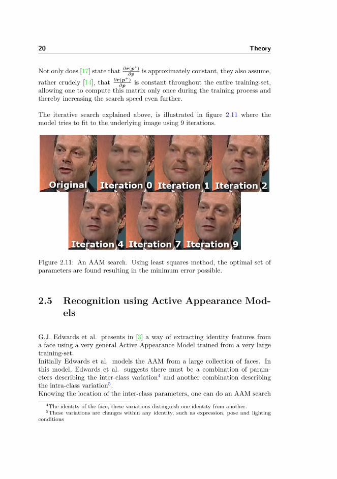
The iterative search explained above, is illustrated in figure 2.11 where themodel tries to fit to the underlying image using 9 iterations.
Figure 2.11: An AAM search. Using least squares method, the optimal set ofparameters are found resulting in the minimum error possible.
2.5 Recognition using Active Appearance Mod-els
G.J. Edwards et al. presents in [3] a way of extracting identity features froma face using a very general Active Appearance Model trained from a very largetraining-set.Initially Edwards et al. models the AAM from a large collection of faces. Inthis model, Edwards et al. suggests there must be a combination of param-eters describing the inter-class variation4 and another combination describingthe intra-class variation5.Knowing the location of the inter-class parameters, one can do an AAM search
4The identity of the face, these variations distinguish one identity from another.5These variations are changes within any identity, such as expression, pose and lighting
conditions
2.6 The Active Appearance Model Threshold 21
on a face and extract these values. Thereby obtaining a vector containing anunique ID for the face. This ID should theoretically be the same for any foto ofthe face.
Another approach to recognize faces, is by modelling a specific AAM to representthe face being searched for. The AAM is then trained from a collection of imagescontaining the face in question. The collection need not be as large as whenmaking a general face model, but must contain common variance to the face suchas expression, pose, lighting conditions and maybe even age-related variation.Such a specific model will be able to match very well to images containing thecorrect face, and based on an overall goodness of fit estimate, one can determineif a face represented by the model is present or not.
2.6 The Active Appearance Model Threshold
When the Active Appearance Software by Mikkel Stegmann [15] has finishedits search, it returns a Mahalanobis Distance measure to indicate the quality ofthe match. This distance measure is calculated in the the truncated principalcomponent space and is defined as:
DM =√
(x− µ)TΣ−1(x− µ) (2.18)
Where x = (x1, x2, x3, ..., xn)T is a set of values describing a point in an n-dimensional space, being compared to a point-distribution with a mean ofµ = (µ1, µ2, µ3, ..., µn)T and a covariance matrix Σ, which is a diagonal ma-trix with the eigenvalues of the principal components in the diagonal.
Assuming that the principal component scores follows a normal distribution,the square the Mahalanobis distance-measure is a sum of squares of indepen-dent identically distributed variables following a normal distribution: N(0, 1).The square of the Mahalanobis distance must therefore follow a χ2 distribution:
D2M = (x− µ)TΣ−1(x− µ) ∈ χ2(n) (2.19)
Stegmann chooses to normalize this distance by dividing with the number ofmodes, n.
22 Theory
D2S = D2
M
n(2.20)
From this, a statistical estimate of a threshold, distinguishing between betweenmembers and non-members of the Active Appearance Model can be computed byfinding an appropriate χ and thereby calculating the corresponding MahalanobisDistance:
D2threshold = χ2
α(v)⇔ (2.21)
Dthreshold =√χ2α(v) = χα(v) (2.22)
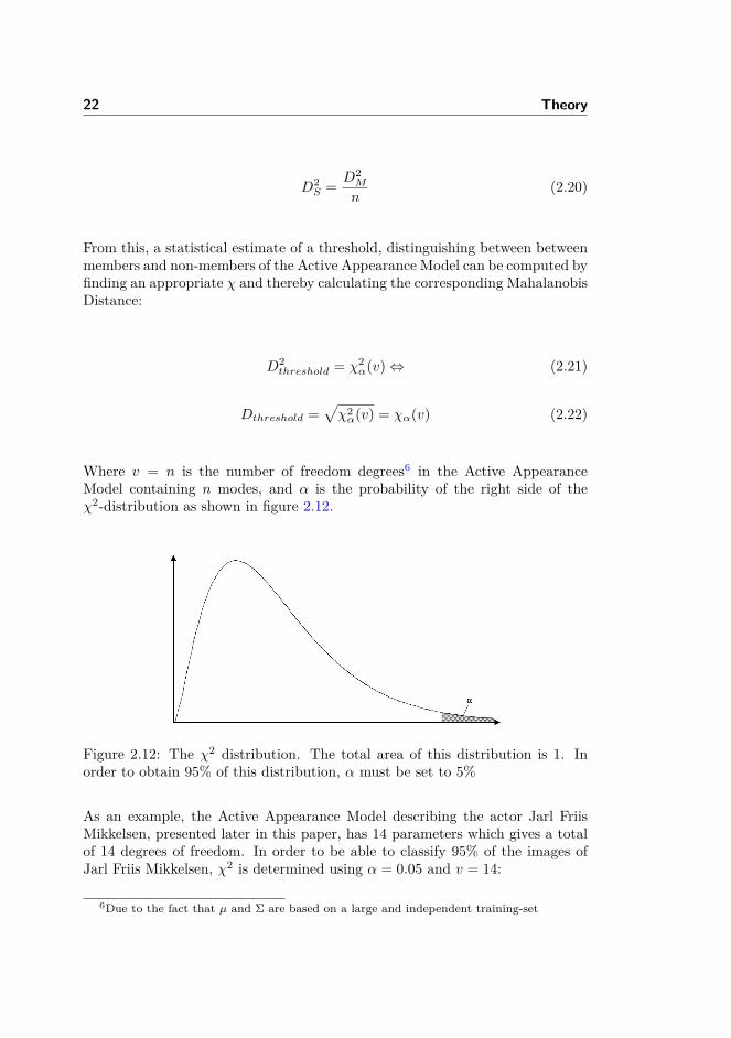
Where v = n is the number of freedom degrees6 in the Active AppearanceModel containing n modes, and α is the probability of the right side of theχ2-distribution as shown in figure 2.12.
Figure 2.12: The χ2 distribution. The total area of this distribution is 1. Inorder to obtain 95% of this distribution, α must be set to 5%
As an example, the Active Appearance Model describing the actor Jarl FriisMikkelsen, presented later in this paper, has 14 parameters which gives a totalof 14 degrees of freedom. In order to be able to classify 95% of the images ofJarl Friis Mikkelsen, χ2 is determined using α = 0.05 and v = 14:
6Due to the fact that µ and Σ are based on a large and independent training-set
2.7 OpenCV 23
D2threshold = χ2
0.05(14)⇔ (2.23)D2threshold = 23.68⇔ (2.24)
D2S,threshold = D2
threshold
n= 23, 68
14 = 1.69⇔ (2.25)
DS,threshold = 1.30 (2.26)
This concludes that theoretically at least 95% of images taken of the subject willbe classified as true, if a Mahalanobis-threshold of 1.30 is used to distinguish.The result of these calculations corresponds nicely to the best threshold foundempirically: 1.2. The threshold was determined by manually tuning in intervalsof 0.1 until the best results were found.
2.7 OpenCV
The procedure of detecting faces using the Viola-Jones algorithm is basically astraight forward task in OpenCV. Among the many other functions, OpenCVcomes with the cvHaarDetectObjects that uses a trained cascade of classifiersto detect an object within the image.
CvSeq* cvHaarDetectObjects(const CvArr* image,CvHaarClassifierCascade* cascade,CvMemStorage* storage,double scale factor=1.1,int min neighbors=3,int flags=0,CvSize min size=cvSize(0,0)
);
The function requires an image, a trained cascade containing Haar-Like Fea-tures7 and allocated memory. The last arguments are optional: Scale factorindicates how much the size of the detection-window should increase after everypass through the image. The neighbors argument groups clusters of detections
7Haar-Like features are the rectangular intensity features described while introducing theViola-Jones algorithm. The features can quickly be calculated in an image using the associatedintegral image as a lookup table.

24 Theory
greater than a given threshold, into one single detection, clusters below thethreshold are discarded. The flags argument only has one option at this mo-ment which is 0, enabling a Canny Edge Detector to discard some areas of theimage that are unlikely to contain the searched object. Finally the size sets theminimum size the detector should search for objects at.When the detection function has been computed it returns a sequence of val-ues, that contain information about the various detections made, including totalcount, specific positions and specific widths and heights.It is obvious that this OpenCV function does the exact operation described byViola-Jones: Scans a range of sub windows using a cascade of weak classifiers,in order to detect a certain object. Therefore, given a well trained classifier cas-cade, this detector can be used to fast and accurately detect faces as proposedby Viola-Jones [19].Before using the cvHaarDetectObjects function, some preparations has to madeon the image in order to maximize the success rate. Firstly the input imagemust be converted into grey scale, since the features are based on light and darkareas. Furthermore Gary Bradski and Adrian Kaehler [1] recommends equaliz-ing the histogram in order to level out the light intensities in the image.After these initial conversions an image is ready for processing. Depending onthe amount of possible faces and the dimensions of the image, the processingtime can vary a lot. In non-HD video footage, where the resolution is fairly low(VHS = 350x480px) this detection process can be computed in real-time on amodern computer.
Chapter 3
Implementation
In this chapter the reflections made, as well as the obstructions faced, duringthe implementation are presented.Due to an unforeseen limitation of the Active Appearance Model software, somenew approaches to the recognition had to be made. This is explained in thefirst section. The following sections concerns how one, using the previously ex-plained theory, in practice snapshots faces from video-footage, builds the ActiveAppearance Model and recognizes faces using the model.
3.1 Limitations of the Active Appearance Modelsoftware
It was expected that the Active Appearance Model software presented by Stegmanet al. [15] was able to output a vector containing the resulting parameters fromthe AAM search. This however was not the case and due the fact that access-ing the API and merging it with this software was beyond the scope of thisproject, another approach to face-recognition using Active Appearance Modelswas taken. Instead it was decided to base the recognition on subject-specificmodels as explained in the previous chapter, knowing that the speed of therecognition-software would be affected.
26 Implementation
3.2 Snapshotting Faces
When processing the video-footage and detecting faces, the software must savekey-snapshots in order to supply the following Active Appearance Model withthe best information available. Basically this means, that every face detectedin a video-sequence must be saved. However, due to the instability of a ViolaJones Detector, this would quickly result in an overflow of snapshots.A way to optimize the snapshot-process, is by utilising the continuity filteringpresented earlier. Theoretically this would allow the software to only take onesnapshot per person present in the footage. Due to some unavoidable breaksin the continuity, such as scene changes or faces turned away from the camera,this is however not possible and one must expect a varying amount of snapshotsper person. Even with these breaks, the method still minimizes the amount ofsnapshots taken greatly though.Another issue is the fact that the Viola Jones Detector does not return a qualityestimate of the face detected. This means that the snapshots saved can be of verypoor quality, and very possibly another and much better face could appear laterwithin the same stream of continuous faces. Therefore one can not only rely ontaking one single snapshot when a face is detected, but must however continuetaking snapshots in certain intervals throughout the span of the detection, inorder to maximize the chance of getting the optimum snapshot of the face.Finally one must secure consistency in the size of snapshots saved, the size offaces within these snapshots, as well as the position of the faces within thesnapshots. This must be done in order to optimize the initialisation the AAM.Luckily the Viola Jones Detector solves two of these problems: The size of facesand the position of faces. Due to the nature of the detector, it will always returnfaces with almost same size and position relative to the window of the detector.With this consistency secured, one can scale and translate the detection windowfreely in order to obtain a snapshot fulfilling the requirements of the AAM (e.g.the jaw must be visible). This is illustrated in fig. 3.1. The last thing to ensure,is the size of the saved snapshots. This is easily done by defining a certainsize, that one wishes all snapshots to be saved in, and then resize snapshotsaccordingly before they are saved.
When implementing the function taking snapshots as explained above, one mustconsider a range of parameters: In what interval should the detector save snap-shots in continuous face-streams? How much must the Viola Jones detectionbe scaled and translated? What dimensions should the saved snapshots have?And finally, in what format should it be saved?In this implementation, the user is able to set a snapshotting interval as well asa cap for the amount of snapshots taken. The default values are snapshots every15th detection (per continuous face) with a maximum of 5 snapshots. In order toincrease recognition-rates the interval and cap can be increased, however, this is

3.2 Snapshotting Faces 27
Figure 3.1: To the left is the raw detection of the Viola Jones Detector. To theright, the faces have been scaled and translated so that all information neededby an AAM is present. Lines has been drawn to illustrate the consistency inscale and position of the detector
on the cost of increased processing time. Concerning the scale and translation,the detection window was scaled 20% larger, moved 5% of the window-heightdownwards and 10% of the width to the left. This scaling and resizing gave thebest results. This is also shown in fig 3.1.The decision about what dimensions the saved snapshot should have, mostlydepends on the size of the images used to train the Active Appearance Model,i.e. there is no need to save images with higher resolution than the one providedby the AAM, on the other hand, one should provide the AAM with images thatcontain enough information, to be able to recognize the face. In this project,a size of 200x200 pixels is used, mostly due to the fact that this is roughly theresolution of the faces in the footage.The format of the saved snapshot basically depends on what formats the AAMprocesses best. Here, the AAM console interface only takes .BMP formats,therefore all snapshots are saved as bitmaps.
28 Implementation
3.3 Building an Active Appearance Model
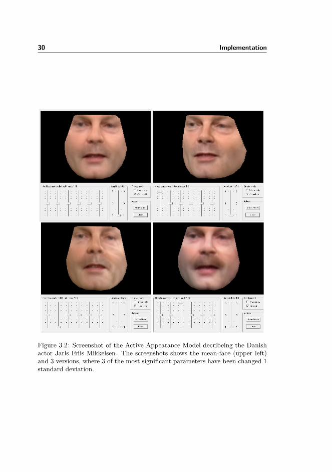
In order to train an Active Appearance Model representing the actor Jarl FriisMikkelsen, a collection of different images of the actor has to be made. All theseimages must show the actors face in different expressions, directions, lightingconditions, as well as additional facial features such as moustache etc. Thisis done in order to ensure that the model is able to match any expression orappearance the actor could be expected to have.In the final Active Appearance Model a total of 29 images was used. Fromthese 29 images, 18 were snapshotted from a piece of video-footage containingthe actor and 11 were found on Google. It was very hard to find proper imagesusing Google, since most images were very biased in pose and expression. Onthe contrary, it was very easy to obtain good images of the actor’s face from thevideo-footage, since a single run of the Viola Jones detector could output a verylarge collection of faces, from which proper images could be hand picked. Thesecond approach is therefore recommended to anyone interested in replicationthis recognition-method.The most time-consuming element in the building-process, was the hand anno-tation of the faces. Could this process be automated as Edwards et al. suggests[17], a lot of man-hours could be saved and the recognition software would bemore or less fully automatic.In figure 3.2 the model is presented, where its 3 most significant parameters arebeing changed.
3.4 Recognition using Active Appearance Mod-els
In the initial recognition tries, a small model only consisting of 15 images wasused to recognize the actor. The recognition proved possible with a MahalanobisDistance Threshold of 2.0. Unfortunately a lot of misclassifications appeareddue to the rather high distance threshold. Extending the model with additionalimages representing the actor improved the recognition considerably. The dis-tance threshold could be lowered to 1.3 which filtered out most of the wrongrecognitions. This indicates that the more trained model one has, the lowerthreshold can be used. However, one must always expect that some false pos-itives can appear. For persons looking very much like the actor, the softwarewill probably not be able to differentiate.Another consideration to do, is whether to average out the Mahalanobis dis-tances per sequence or simply classify using the lowest distance found. Theoret-ically the model should only fit perfect to the subject it is trained for thereby

3.4 Recognition using Active Appearance Models 29
resulting in a very low Mahalanobis distance, but due to different sorts of noisein video-footage, one could expect that a multiple snapshots of the subjectwould be obscured by the noise and would in fact pull the distance-averageabove the distance-threshold. Classification based on lowest score is thereforea good approach and is implemented as the standard classification method inthis software. It can of course be changed to be based on the average-distanceinstead if the user wishes this.One major issue at this point, is the fact that the AAM-search is rather slow. Anaverage search on a 200x200 pixel image takes 1.5 seconds. When using the de-fault snapshotting settings in the software, there are roughly taken 60 snapshotsper minute in interview-like footage. This results in a rather long processingtime afterwards ≈ 1.5 minutes of processing per minute of video-footage. Sincethe processing time by the AAM-search is probably not very optimizable, themajor improvements could probably instead be found in the way the snapshotsare taken. Lowering the limit to the amount of snapshots taken of a continu-ous face or increasing the interval between every snapshot, could be one wayforward. However, every time the amount of snapshots is decreased, the oddsof having a good quality face-image is also decreased. Therefore one should becareful not to decrease the amount of snapshots too much.
30 Implementation
Figure 3.2: Screenshot of the Active Appearance Model decribeing the Danishactor Jarls Friis Mikkelsen. The screenshots shows the mean-face (upper left)and 3 versions, where 3 of the most significant parameters have been changed 1standard deviation.

Chapter 4
Results and Discussion
In this chapter the performance of the recognition software will be described inform of test results. Initially the detection performance will be presented andsubsequently the recognition performance. Finally will the results be discussed.
4.1 Detection Results
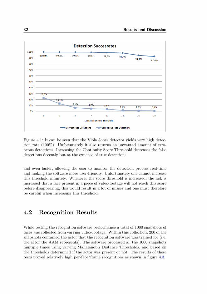
In order to test the performance of the Viola Jones Detector with the ContinuityFilter applied a set of sequences were picked containing a total of 700 frames.The face detection results are presented in figure 4.1, where it can be seenclearly, that the filter radically reduces the false detections while maintaining avery high detection rate.
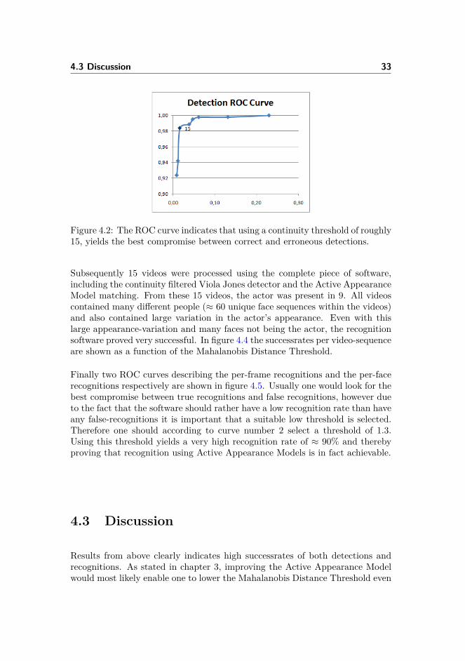
In order to get an indication of what continuity threshold should be used, aROC curve is also presented in figure 4.2. This curve is generated from thesame collection of data and indicates that the optimum threshold lies around15.
Not only has the detector and filter proven very high detection rates, but alsothe speed of the detector and filter combined is mentionable. Even with thefilter applied, the detector is still able to process video-streams in real-time
32 Results and Discussion
Figure 4.1: It can be seen that the Viola Jones detector yields very high detec-tion rate (100%). Unfortunately it also returns an unwanted amount of erro-neous detections. Increasing the Continuity Score Threshold decreases the falsedetections decently but at the expense of true detections.
and even faster, allowing the user to monitor the detection process real-timeand making the software more user-friendly. Unfortunately one cannot increasethis threshold infinitely. Whenever the score threshold is increased, the risk isincreased that a face present in a piece of video-footage will not reach this scorebefore disappearing, this would result in a lot of misses and one must thereforebe careful when increasing this threshold.
4.2 Recognition Results
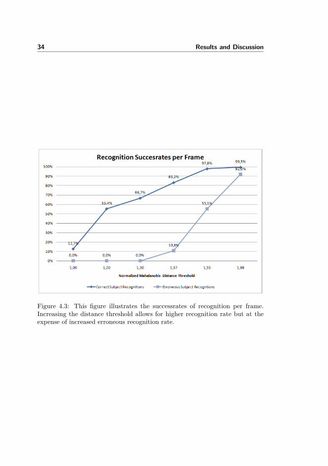
While testing the recognition software performance a total of 1000 snapshots offaces was collected from varying video-footage. Within this collection, 200 of thesnapshots contained the actor that the recognition software was trained for (i.e.the actor the AAM represents). The software processed all the 1000 snapshotsmultiple times using varying Mahalanobis Distance Thresholds, and based onthe thresholds determined if the actor was present or not. The results of thesetests proved relatively high per-face/frame recognitions as shown in figure 4.3.
4.3 Discussion 33
Figure 4.2: The ROC curve indicates that using a continuity threshold of roughly15, yields the best compromise between correct and erroneous detections.
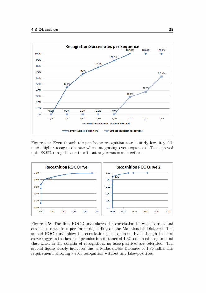
Subsequently 15 videos were processed using the complete piece of software,including the continuity filtered Viola Jones detector and the Active AppearanceModel matching. From these 15 videos, the actor was present in 9. All videoscontained many different people (≈ 60 unique face sequences within the videos)and also contained large variation in the actor’s appearance. Even with thislarge appearance-variation and many faces not being the actor, the recognitionsoftware proved very successful. In figure 4.4 the successrates per video-sequenceare shown as a function of the Mahalanobis Distance Threshold.
Finally two ROC curves describing the per-frame recognitions and the per-facerecognitions respectively are shown in figure 4.5. Usually one would look for thebest compromise between true recognitions and false recognitions, however dueto the fact that the software should rather have a low recognition rate than haveany false-recognitions it is important that a suitable low threshold is selected.Therefore one should according to curve number 2 select a threshold of 1.3.Using this threshold yields a very high recognition rate of ≈ 90% and therebyproving that recognition using Active Appearance Models is in fact achievable.
4.3 Discussion
Results from above clearly indicates high successrates of both detections andrecognitions. As stated in chapter 3, improving the Active Appearance Modelwould most likely enable one to lower the Mahalanobis Distance Threshold even
34 Results and Discussion
Figure 4.3: This figure illustrates the successrates of recognition per frame.Increasing the distance threshold allows for higher recognition rate but at theexpense of increased erroneous recognition rate.
4.3 Discussion 35
Figure 4.4: Even though the per-frame recognition rate is fairly low, it yieldsmuch higher recognition rate when integrating over sequences. Tests provedupto 88.9% recognition rate without any erroneous detections.
Figure 4.5: The first ROC Curve shows the correlation between correct anderroneous detections per frame depending on the Mahalanobis Distance. Thesecond ROC curve show the correlation per sequence. Even though the firstcurve suggests the best compromise is a distance of 1.37, one must keep in mindthat when in the domain of recognition, no false-positives are tolerated. Thesecond figure clearly indicates that a Mahalanobis Distance of 1.30 fulfils thisrequirement, allowing ≈90% recognition without any false-positives.

36 Results and Discussion
further, as well as allowing better matching of images containing the actor. Thiswould increase successrates even further while keeping the false recognitions atzero and is therefore a good way of improving the software.Even though the recognition results looks promising, one must keep in mindthat the statistics are based on a fairly small set of data. In order to properlytest this software, even more sample videos of the actor are required as well asfootage not containing him. The charts presented in this chapter are thereforenot fully trustworthy and should only be compared to the data that was avail-able.The speed of the AAM software is one major disadvantage at this point. Al-though the actual search algorithm is not optimizable, the fact that the searchis performed on all snapshots of a face-sequence, and not stopped whenevera score is lower than the threshold, is an issue. This is caused by the AAMsoftware that does not return any Mahalanobis-distances before all images havebeen processed. If one merged the AAM API into this software, much morespecific AAM-calls could be performed, allowing the searches to stop whenevera match is found and thereby lowering the processing time greatly. Usage of theAPI would also allow for parameter based recognition as previously presented.With this said, one must keep in mind that not all footage is as face-intense asthe footage that has been tested here. All of this footage consisted of interview-like material with a constant presence of faces. In many scenarios much lessface-intensity will probably be present, resulting in less processing time by thesoftware. Also as processing power of computers is constantly increasing, onecould expect that this matter is not any issue in just a few years.Implementation of the Kalman Filter combined with a scene-change-detectormight also help reduce some of the splitting of face-sequences happening when-ever a face-tracking is lost due to for example head-turning or a hand coveringthe face. This would likely reduce the amount of snapshots to be processed andthereby reduce the processing time even further.Finally it must be mentioned, as it has been briefly in the Implementation Chap-ter, that the manual annotation of faces for the Active Appearance Model is avery time-consuming process. Semi- or full-automation of this process would bea major improvement. An approach to this, could be building a super-generalface model from a very large training set. Letting this very flexible modelfit onto a collection of images describing the subject for the recognition-AAMwould yield automatic annotation and allow for automatic building of AAMs,by only supplying a collection of faces. Of course this requires the constructionof a massive AAM, but this only needs to be done a single time. Moreover themodel can be built in steps allowing it to aid its own training-process.
Chapter 5
Conclusion
5.1 Conclusion
Using the OpenCV C-programming package, a continuity filtered Viola Jonesface-detector was successfully implemented. The detector obtained a successrateof 98% with a reduction of erroneous detections from 30% down to 1.6%. Wethereby directly proved that continuity filtering is able to remove the majorityof all noise present in the Viola Jones detector.Subsequently we successfully proved that Active Appearance Models are veryapplicable in the domain of face-recognition and that recognition rates close to90% are achievable. Even though our implementation only contained 1 ActiveAppearance Model, the concept allows for the use of multiple models in orderto do white-list matches as indicated in the problem statement.
5.2 Future Work
As stated in previous chapter, an integration of the AAM framework wouldallow for even faster recognition as well as open up for the possibility of doingparameter-based recognition as suggested by Edwards et al. [3]. Therefore this

38 Conclusion
is an obvious place to optimize this solution. Another upgrade mentioned isthe automatization of the AAM training, if this was implemented, the softwarewould become much more user-friendly and would not require any preparationsbefore recognition.Aside from the above examples of improvements, one final obvious optimizationis simply optimizing the already written code.

Appendix A
Test Data
In tables A.1, A.2, A.3 and A.4 test results concerning the Viola Jones FaceDetector are presented. In these tests the continuity Score Threshold was in-creased.Afterwards in tables A.5, A.6 and A.7 the test results from per-face recognitionsare presented. In these tests the Mahalanobis Distance Threshold was increased.Finally in tables A.8, A.9, A.10 and A.11 the overall recognition test results arepresented. Also here the Mahalanobis Distance Threshold was increased.
Table A.1: Viola Jones Detections, part 1
Minimum Score: 1 Minimum Score: 2
Faces found 517 Faces found 476Faces not found: 0 Faces not found: 1
Wrong detections: 154 Wrong detections: 72Total detections: 671 Total detections: 549
Total faces: 517 Total faces: 477Hit %: 100,0% Hit %: 99,8%
Error %: 23,0% Error %: 13,1%

40 Test Data
Table A.2: Viola Jones Detections, part 2
Minimum Score: 5 Minimum Score: 7
Faces found 444 Faces found 405Faces not found: 1 Faces not found: 2
Wrong detections: 29 Wrong detections: 20Total detections: 474 Total detections: 427
Total faces: 445 Total faces: 407Hit %: 99,8% Hit %: 99,5%
Error %: 6,1% Error %: 4,7%
Table A.3: Viola Jones Detections, part 3
Minimum Score: 10 Minimum Score: 15
Faces found 347 Faces found 303Faces not found: 4 Faces not found: 5
Wrong detections: 14 Wrong detections: 5Total detections: 365 Total detections: 313
Total faces: 351 Total faces: 308Hit %: 98,9% Hit %: 98,4%
Error %: 3,8% Error %: 1,6%
Table A.4: Viola Jones Detections, part 4
Minimum Score: 20 Minimum Score: 25
Faces found 244 Faces found 218Faces not found: 15 Faces not found: 18
Wrong detections: 3 Wrong detections: 2Total detections: 262 Total detections: 238
Total faces: 259 Total faces: 236Hit %: 94,2% Hit %: 92,4%
Error %: 1,1% Error %: 0,8%

41
Table A.5: Recognition per frame, part 1
Excluded % 45,00% Excluded % 13,00%Number of Modes: 14,00 Number of Modes: 14,00
Mahalanobis Distance: 1,00 Mahalanobis Distance: 1,20
Stats: Stats:Total TrueFalse: 418,00 Total TrueFalse: 418,00Total TrueTrue: 26,00 Total TrueTrue: 113,00Total FalseTrue: 0,00 Total FalseTrue: 0,00Total FalseFalse: 178,00 Total FalseFalse: 91,00Times present: 204,00 Times present: 204,00
Times not present: 418,00 Times not present: 418,00Hit %: 12,7% Hit %: 55,4%
Erroneous Detection %: 0,0% Erroneous Detection %: 0,0%
Table A.6: Recognition per frame, part 2
Excluded % 5,00% Excluded % 2,50%Number of Modes: 14,00 Number of Modes: 14,00
Mahalanobis Distance: 1,30 Mahalanobis Distance: 1,37
Stats: Stats:Total TrueFalse: 418,00 Total TrueFalse: 373,00Total TrueTrue: 136,00 Total TrueTrue: 153,00Total FalseTrue: 0,00 Total FalseTrue: 45,00Total FalseFalse: 68,00 Total FalseFalse: 31,00Times present: 204,00 Times present: 184,00
Times not present: 418,00 Times not present: 418,00Hit %: 66,7% Hit %: 83,2%
Erroneous Detection %: 0,0% Erroneous Detection %: 10,8%
42 Test Data
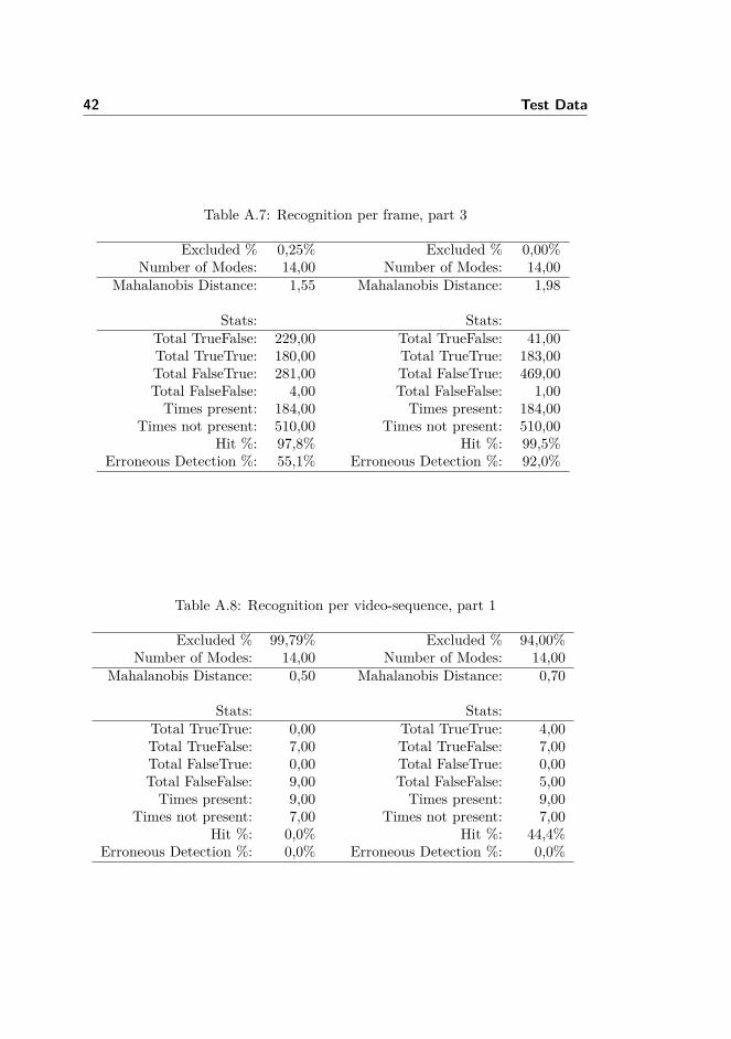
Table A.7: Recognition per frame, part 3
Excluded % 0,25% Excluded % 0,00%Number of Modes: 14,00 Number of Modes: 14,00
Mahalanobis Distance: 1,55 Mahalanobis Distance: 1,98
Stats: Stats:Total TrueFalse: 229,00 Total TrueFalse: 41,00Total TrueTrue: 180,00 Total TrueTrue: 183,00Total FalseTrue: 281,00 Total FalseTrue: 469,00Total FalseFalse: 4,00 Total FalseFalse: 1,00Times present: 184,00 Times present: 184,00
Times not present: 510,00 Times not present: 510,00Hit %: 97,8% Hit %: 99,5%
Erroneous Detection %: 55,1% Erroneous Detection %: 92,0%
Table A.8: Recognition per video-sequence, part 1
Excluded % 99,79% Excluded % 94,00%Number of Modes: 14,00 Number of Modes: 14,00
Mahalanobis Distance: 0,50 Mahalanobis Distance: 0,70
Stats: Stats:Total TrueTrue: 0,00 Total TrueTrue: 4,00Total TrueFalse: 7,00 Total TrueFalse: 7,00Total FalseTrue: 0,00 Total FalseTrue: 0,00Total FalseFalse: 9,00 Total FalseFalse: 5,00Times present: 9,00 Times present: 9,00
Times not present: 7,00 Times not present: 7,00Hit %: 0,0% Hit %: 44,4%
Erroneous Detection %: 0,0% Erroneous Detection %: 0,0%
43
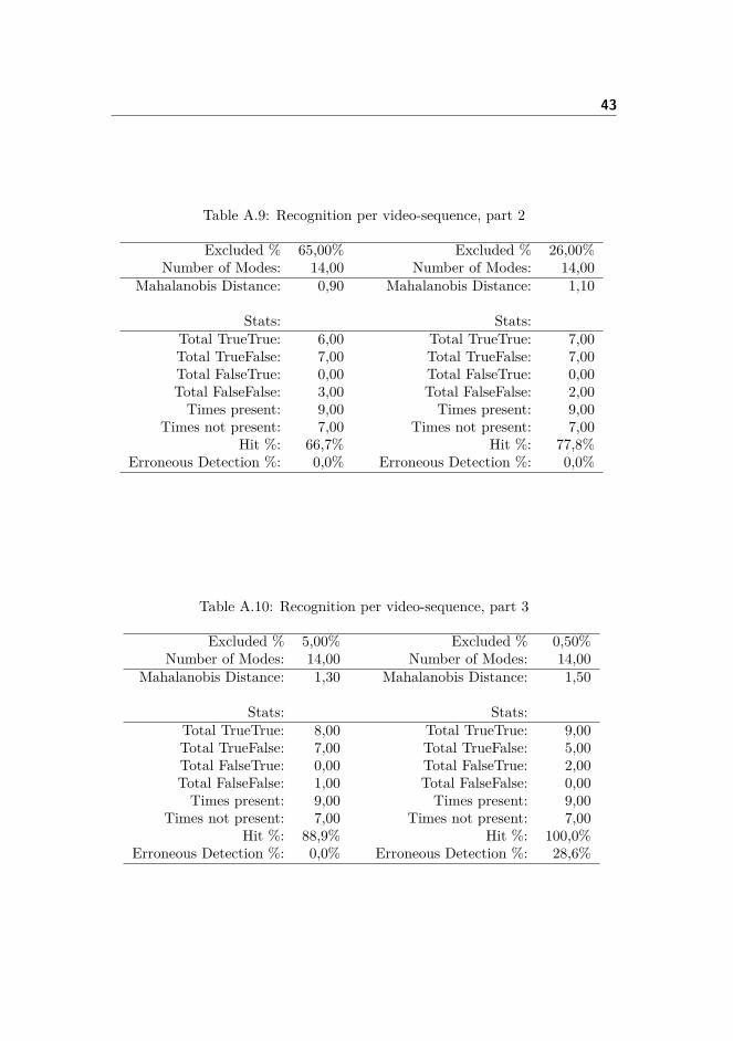
Table A.9: Recognition per video-sequence, part 2
Excluded % 65,00% Excluded % 26,00%Number of Modes: 14,00 Number of Modes: 14,00
Mahalanobis Distance: 0,90 Mahalanobis Distance: 1,10
Stats: Stats:Total TrueTrue: 6,00 Total TrueTrue: 7,00Total TrueFalse: 7,00 Total TrueFalse: 7,00Total FalseTrue: 0,00 Total FalseTrue: 0,00Total FalseFalse: 3,00 Total FalseFalse: 2,00Times present: 9,00 Times present: 9,00
Times not present: 7,00 Times not present: 7,00Hit %: 66,7% Hit %: 77,8%
Erroneous Detection %: 0,0% Erroneous Detection %: 0,0%
Table A.10: Recognition per video-sequence, part 3
Excluded % 5,00% Excluded % 0,50%Number of Modes: 14,00 Number of Modes: 14,00
Mahalanobis Distance: 1,30 Mahalanobis Distance: 1,50
Stats: Stats:Total TrueTrue: 8,00 Total TrueTrue: 9,00Total TrueFalse: 7,00 Total TrueFalse: 5,00Total FalseTrue: 0,00 Total FalseTrue: 2,00Total FalseFalse: 1,00 Total FalseFalse: 0,00Times present: 9,00 Times present: 9,00
Times not present: 7,00 Times not present: 7,00Hit %: 88,9% Hit %: 100,0%
Erroneous Detection %: 0,0% Erroneous Detection %: 28,6%

44 Test Data
Table A.11: Recognition per video-sequence, part 4
Excluded % 0,02% Excluded % 0,00%Number of Modes: 14,00 Number of Modes: 14,00
Mahalanobis Distance: 1,70 Mahalanobis Distance: 1,90
Stats: Stats:Total TrueTrue: 9,00 Total TrueTrue: 9,00Total TrueFalse: 5,00 Total TrueFalse: 3,00Total FalseTrue: 3,00 Total FalseTrue: 5,00Total FalseFalse: 0,00 Total FalseFalse: 0,00Times present: 9,00 Times present: 9,00
Times not present: 8,00 Times not present: 8,00Hit %: 100,0% Hit %: 100,0%
Erroneous Detection %: 37,5% Erroneous Detection %: 62,5%

Appendix B
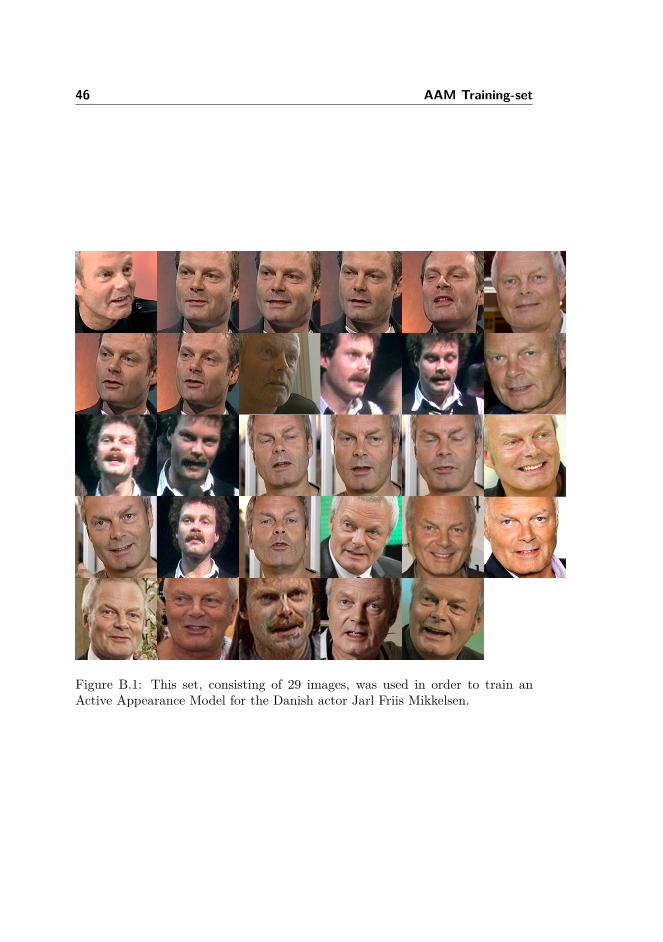
AAM Training-set
Figure B.1 presents the 29 images that were used in order to built the Appear-ance Model Representing the Danish actor Jarl Friis Mikkelsen.
46 AAM Training-set
Figure B.1: This set, consisting of 29 images, was used in order to train anActive Appearance Model for the Danish actor Jarl Friis Mikkelsen.

Appendix C
Software Manual
The software can be downloaded from:
http://www.Boll-Nielsen.dk/FaceRecognition.zip
This zip file contains the full software including C-code and a sample-video.
For the software to build Active Appearance Models as well as the full AAMFramework, please visit:
http://www.imm.dtu.dk/~aam/
C.1 Calling the Software
There are two ways of calling the software. The first and most intuitive be-ing simply running the Detector.exe and entering a path to a video-file whenprompted. Another method is by calling the Detector.exe from the commandprompt with the first argument being the path to the video-file:
"path/to/detector/detector.exe video/path.avi"

48 Software Manual
The software accepts both .AVI and .MPEG formats.During face-detection, pressing escape stops the face-detection procedure andforces the software to recognize using only the detections made until escape waspressed.
C.2 Changing the Settings
In order to change the detection and recognition parameters, one can access theSettings.rsf file. This file contains a list of settings allowing one to customizethe software to a specific task. Here, one can also change the Detection Cas-cade and the Active Appearance Model, this enables the software to deal withrecognition-tasks not necessarily related to face-recognition since any detectorand appearance model can be taken into use.
C.3 Reading the Output
After the software has processed video-footage it informs the user if the subjectwas present and if so, it will also output timestamps about the subjects appear-ance.If one is interested in a more detailed insight in the recognition process, a filenamed Detections.txt will be created after every run, allowing one to see thecomplete collection of Mahalanobis Distances calculated. Also snapshots takenby the software are accessible, all snapshots are placed in the processing/folder together with their associated AAM-matches.
C.4 Known bugs
If a grey-scale Active Appearance Model is taken into use, it is very importantthat grey-scale mode is also activated in the settings (or vice versa). If this isnot done, the software will crash.
Too long or too face-intensive video-footage can cause the software to reachthe maximum amount of face-detections allowed, resulting in memory-allocationerrors during the detection phase. To avoid this, one should check that a rea-sonably high Continuity Filtering Threshold is being used. If the error persists,one can split the video-sequence into smaller sequences.

C.4 Known bugs 49
In very rare cases the Active Appearance Model Software encounters image-regions that it is not able to process properly. This results in the softwarecrashing during the recognition phase. In order to avoid this error, one canchange the snapshotting-intervals or continuity threshold in the settings andthereby prevent the software from snapshotting that specific frame again.
If a crash cannot be solved using the above solutions, ensure that the correctfiles and folders exists in the software folder:
processing/Data/
jarlmodel.amfhaarcascade_frontalface_alt2.xml
Detector.exeSettings.rsfaamc.exeaamcm.execv200.dllcvaux200.dllcxcoer200.dllcxts200.dllhighgui200.dllml200.dllopencv_ffmpeg200.dllVisCore.dllVisMatrix.dllVisXCLAPACK.dll
If any of these files or folders are missing, the software will not run properly. Ifthis is the case, please redownload the software from the url in the start of thisappendix.

50 Software Manual

Bibliography
[1] Gary Bradski and Adrian Kaebler. Learning OpenCV - Computer Visionwith the OpenCV Library. O’Reilly, 2008.
[2] Jens Michael Carstensen, editor. Image Analysis, Vision and ComputerGraphics. Technical University of Denmark, 2002.
[3] T.F. Cootes G.J. Edwards and C.J. Taylor. Face recognition using activeappearance models. Technical report, University of Manchester.
[4] Shumeet Baluja Henry A. Rowley and Takeo Kanade. Neural network-based face detection. Technical report, 1998.
[5] G. Toderici N. Murtuza I. Kakadiaris, G. Passalis and T. Theoharis. 3dface recognition. Technical report, University of Athens, Greece.
[6] Open Source Intel. http://opencv.willowgarage.com/wiki/. 1999.
[7] Ole Helvig Jensen. Implementing the viola-jones face detection algorithm.Master’s thesis, DTU, 2008.
[8] Richard Johnson, editor. Probability and Statistics for Engineers. PearsonEducation, inc, 1965.
[9] Better Face-Recognition Software Mark Williams.http://www.technologyreview.com/Infotech/18796/?a=f. 2008.
[10] Charlie McDowell, editor. On to C. Addison Wesley, 2001.
[11] Henry Schneiderman and Takeo Kanade. A statistical method for 3d objectdetection applied to faces and cars. Technical report, Carnegie MellonUniversity.

52 BIBLIOGRAPHY
[12] Naotoshi Seo. http://note.sonots.com/SciSoftware/haartraining.html.2008.
[13] L-1 Identity Solutions. http://www.l1id.com/. 2009.
[14] M. B. Stegmann. Analysis and segmentation of face images using pointannotations and linear subspace techniques. Technical report, Informat-ics and Mathematical Modelling, Technical University of Denmark, DTU,Richard Petersens Plads, Building 321, DK-2800 Kgs. Lyngby, 2002.
[15] M. B. Stegmann, B. K. Ersbøll, and R. Larsen. FAME – a flexibleappearance modelling environment. IEEE Trans. on Medical Imaging,22(10):1319–1331, 2003.
[16] NSTC Subcommittee. Face recognition. Technical report, National Scienceand Technology Counsil (NSTC), 2006.
[17] Gareth J. Edwards Timothy F. Cootes and Christopher J. Taylor. Activeappearance models. In IEEE Transactions on Pattern Analysis and MachineIntelligence.
[18] M. Turk and A. Pentland. Face recognition using eigenfaces. Technicalreport, Massachusetts Institute of Technology, 1999.
[19] Paul Viola and Michael Jones. Robust real-time object detection. Technicalreport, July 2001.


![2D Face Detection and Recognition MSc [I.T].docx](https://img.pdfslide.us/doc/110x75/55cf8f31550346703b99d484/2d-face-detection-and-recognition-msc-itdocx.jpg)


![Face Detection & Face Recognition [Teori Informasi 2011]](https://img.pdfslide.us/doc/110x75/548258a6b07959570c8b476a/face-detection-face-recognition-teori-informasi-2011.jpg)