Fabular: Regression Formulas as Probabilistic Programming

Johannes BorgströmUppsala University

Sweden

Andrew D. GordonMicrosoft Research andUniversity of Edinburgh

UK

Long OuyangStanford University

USA

Claudio RussoMicrosoft Research

UK

Adam ScibiorUniversity of Cambridge and

MPI TübingenGermany

Marcin SzymczakUniversity of Edinburgh

UK

AbstractRegression formulas are a domain-specific language adopted byseveral R packages for describing an important and useful classof statistical models: hierarchical linear regressions. Formulas aresuccinct, expressive, and clearly popular, so are they a useful ad-dition to probabilistic programming languages? And what do theymean? We propose a core calculus of hierarchical linear regression,in which regression coefficients are themselves defined by nestedregressions (unlike in R). We explain how our calculus captures theessence of the formula DSL found in R. We describe the design andimplementation of Fabular, a version of the Tabular schema-drivenprobabilistic programming language, enriched with formulas basedon our regression calculus. To the best of our knowledge, this is thefirst formal description of the core ideas of R’s formula notation,the first development of a calculus of regression formulas, and thefirst demonstration of the benefits of composing regression formu-las and latent variables in a probabilistic programming language.

Categories and Subject Descriptors D.3.2 [Programming Lan-guages]: Language Classifications—Specialized application lan-guages; I.2.6 [Artificial Intelligence]: Learning—Parameter Learn-ing

Keywords Bayesian inference; linear regression; probabilisticprogramming; relational data; hierarchical models

1. IntroductionOur goal is to embrace and extend R’s hugely popular regressionformulas to get better probabilistic programming languages.

1.1 Background: R’s Regression FormulasThe R statistical programming language allows notation of the formy∼ x to express linear regression models. If xi,yi are the data in rowi of a table, this model expresses that each yi = α +βxi + ei whereei is an error term. Given this data and model, the regression task is

to learn the global parameters α and β , the intercept and the slopeof the line, by statistical inference.

While this example is an elementary univariate regression, thedomain-specific languages of R formulas, as implemented by sev-eral different inference packages, support a wide range of classes ofregressions (including multivariate, hierarchical, and generalized).The notation anonymises the parameters, such as α and β , has use-ful defaults, such as including the intercept and error terms auto-matically, and hence is extremely succinct.

Still, the published descriptions of R formulas are informal andnon-compositional. If we are to transplant R formulas to other lan-guages, the first problem is to obtain precise syntax and semantics.

1.2 Background: Probabilistic ProgrammingA system for probabilistic programming (Goodman 2013; Gordonet al. 2014b) asks the user to provide a probabilistic model as apiece of code, and provides a compiler to generate efficient codefor statistical inference. Following the earliest system BUGS (Gilkset al. 1994; Lunn et al. 2013), there are many systems, includingBLOG (Milch et al. 2007), Infer.NET (Minka et al. 2009), Church(Goodman et al. 2008), Figaro (Pfeffer 2009), HANSEI (Kiselyovand Shan 2009), Fun (Borgström et al. 2013), Stan (Stan Develop-ment Team 2014a), R2 (Nori et al. 2014), Anglican (Wood et al.2014), Probabilistic C (Paige and Wood 2014), Venture (Mans-inghka et al. 2014), and Wolfe (Riedel et al. 2014).

From the start, BUGS, Stan, and other languages have been ap-plied to hierarchical models, but written as explicit nested loopsover the data. To the best of our knowledge, no previous proba-bilistic programming language has adopted R’s formula notation.

1.3 Part 1: Regression Calculus for Hierarchical ModelsIn their classic textbook, Gelman and Hill (2007) define a hierarchi-cal/multilevel model to be “a regression (a linear or generalized lin-ear model) in which the parameters—the regression coefficients—are given a probability model.” Their textbook uses R formulas forsimple regressions, but since there is no R notation for definingpriors on coefficients or for directly describing hierarchical mod-els, Gelman and Hill use probabilistic programs (in BUGS) whendescribing hierarchical models with priors.

Calculus of Hierarchical Regression The purpose of our regres-sion calculus is to be a precise notation for hierarchical models withexplicit priors for coefficients, and with default choices of priors toretain the succinctness of R formulas. Our calculus is inspired byR formulas and translates to probabilistic programs (in Fun, but

This is the author’s version of the work. It is posted here for your personal use. Not forredistribution. The definitive version was published in the following publication:

POPL’16, January 20–22, 2016, St. Petersburg, FL, USAc© 2016 ACM. 978-1-4503-3549-2/16/01...

http://dx.doi.org/10.1145/2837614.2837653

271

easily adapted to BUGS). A unique feature in our calculus is thecoefficient regression v{α ∼ r}, which introduces a coefficient α

together with its nested probability model r, directly correspondingto Gelman and Hill’s definition of a hierarchical model.

Section 2 introduces the syntax and informal semantics of ourregression calculus via a series of examples. Section 4 completesthe exposition by explaining more complex examples.

Section 3 presents the standard Bayesian interpretation of re-gression via our calculus. We recall Fun as a syntax for interpretingregressions as typed probabilistic programs, themselves formalisedin measure theory. Theorem 1 (Type Preservation) guarantees thateach well-typed regression maps to a well-typed Fun expression,and hence is interpreted as a measure over the measurable spacefor its type. Hence, for any well-typed regression y ∼ r we definethe prior distribution on its parameters and the output column ofdata for y; and conditioned on observed data Vy possibly with miss-ing values, we define the posterior distribution on its parametersand output, which yields predictions for the missing values.

Our calculus has new features beyond R’s regression formulas:

(1) The coefficient construct v{α ∼ r} is a nested syntax for hier-archical linear models. R has no nested syntax for models.

(2) We can set priors for coefficients such as slopes, intercepts, orthe precision of error terms.

(3) Input and output data and parameters are all typed.

Flattening Multilevel Formulas to Single Level A hierarchicalregression such as (1{α ∼ rα} | s) + x{β ∼ rβ } includes subex-pressions rα and rβ that model the parameters α and β (here, the |ssyntax after {α ∼ rα} indicates that we will have one α for everyvalue of the categorical variable s). The regressions rα and rβ maythemselves include nested coefficients on group-level input data. InSection 5 we recall Gelman and Hill’s discussion of how a hierar-chical regression may be re-arranged so there are no nested coeffi-cients, and by accessing group-level data from the top-level. Theo-rem 2 establishes that any well-typed regression has an equivalentsingle-level counterpart. Still, the advantage of our calculus overflattened formulas in R is that hierarchical syntax better reflects theintended structure of the model.

Explaining R’s Regression Formulas We developed our calculusto be a core language to explain the regression formulas of R. Sec-tion 6 describes a semantics for the formula dialects implementedby lm, lmer, and blmer by mapping to the regression calculus.

1.4 Part 2: Fabular = Tabular + Regression CalculusTabular (Gordon et al. 2014a, 2015) is a schema-driven probabilis-tic programming language embedded in a spreadsheet, with infer-ence by Infer.NET (Minka et al. 2009). In Section 7, we extendTabular with columns defined by regressions from the regressioncalculus. Hence, we can express hierarchical models. In addition,since Tabular, like most probabilistic programming languages, sup-ports latent variables defined by a model, we can use formulas toexpress models based on latent variables, such as clustering or rank-ing models. Moreover, we adopt a vectorized interpretation of re-gressions, where coefficients and outputs are vectors; hence, weobtain a formula notation for vector-based models. We developin detail the bilinear recommender model Matchbox (Stern et al.2009). We report a list of Fabular models we have running withinthe spreadsheet environment.

Formulas in Fabular have all the power of the regression calcu-lus, and go beyond R in allowing:

(1) Use of latent variables, either continuous (such as abilities) ordiscrete (such as mixture components for clustering).

(2) Vectorized interpretation for examples such as Matchbox.

Section 8 concludes the paper. Technical report (Borgströmet al. 2015) contains more details, definitions and proofs.

1.5 Contributions of the PaperWe propose the first formal calculus of regressions, with a uniquerecursive syntax for hierarchical models (based on the coefficientconstruct v{α ∼ r}), and a rigorous typed semantics. We developa semantic equivalence for regressions, which we apply to trans-form multilevel regressions to equivalent single-level regressions.We explain the essence of the popular formula notation in R’s lm,lmer, and blmer by converting formulas to terms of the regres-sion calculus. To our knowledge, this is the first formal descriptionof the core ideas of R’s formula notation. We design and imple-ment Fabular, a version of the Tabular schema-driven probabilisticprogramming language that is enriched with formulas from our re-gression calculus.

1.6 Related WorkWe discussed probabilistic programming systems in Section 1.2.Morandat et al. (2012) conduct a careful analysis of the design ofthe R programming language, but do not consider its formula no-tation for regression. There are informal descriptions of R formu-las such as (Hahn) and in the documentation for R packages. Forexample, Bates et al. (2014) provide a careful description of thesemantics of lmer formulas in terms of matrix representations andalgorithms. In addition, they detail instructive examples of a varietyof lmer formulas but do not provide a grammar for this languageor discuss the precise semantics of the syntax.

2. A Core Calculus of Regression, by ExampleWe give the syntax and informal semantics of the regression calcu-lus, together with a series of examples. The formal typing rules andsemantics are in Section 3.

2.1 Syntax and Informal SemanticsThe types of the calculus are real, bounded naturals mod(n) forn≥ 0, and sized array types. Let s range over real constants.

Variables, Naming Conventions, and Types:T,U ::= real |mod(n) | T [n] type (n≥ 0)x,y (continuous real) c,d (categorical mod(n)) α,β ,π (parameter)Γ ::= x1 : T1, . . . ,xn : Tn xi distinct type environment

A core idea of the calculus is that expressions denote probabil-ity distributions over multidimensional arrays of data, referred to ascubes. A cube may be a column of predicted data, a single param-eter (a zero-dimensional array), an array or a doubly-indexed arrayof parameters. (Higher dimensions are possible.)

Dimensions and Cube-Expressions:

Let a dimension,~e or ~f , be a finite list of natural numbers.Let a cube-expression with dimension~e = [e1; . . . ;en] be a phrasethat denotes a multi-dimensional array of some type T [en] . . . [e1].An index for~e is a list [i1; . . . ; in] with 0≤ i j < e j for each j.

A predictor v is a (deterministic) cube-expression made up ofconstants, variables, interactions, and paths.

Syntax of Predictors:u,v ::= predictor

s scalar (common cases are 1 and 0)x variable (categorical or continuous)u : v interaction (multiplication)(u1, . . . ,un).v path

272

A scalar s returns the cube with s at each index. A variablex returns the cube denoted by x. An interaction u : v is the pair-wise multiplication of u and v; it returns the cube with v[~i]× u[~i]at each index~i. Finally, a path (u1, . . . ,un).v computes an interme-diate [ f1; . . . ; fn]-cube for v, computes cubes u1, . . . , un containingindexes for dimensions f1, . . . , fn, and returns the cube obtained byapplying the indexes from u1, . . . , un to v. For instance, the form().v allows a []-dimensional cube v (that is, a scalar) to be mappedto a cube of arbitrary dimension. We write u1.v for (u1).v.

A regression r is a probabilistic cube-expression that returns atuple of static parameters alongside a cube of outputs.

Syntax of Regressions:r ::= regression

D(v1, . . . ,vn) noise with distribution Dv{α ∼ r} predictor with coefficientr+ r′ sumr | v grouping(να)r restriction (scope of α is r)

A noise term D(v1, . . . ,vn) returns a cube with an independentrandom draw from the distribution D(v1[~i], . . . ,vn[~i]) at each in-dex [~i]. We assume the following families D of distributions.

Distributions: D : (y1 : U1, . . . ,yn : Un)→ T

Dirac : (point : T )→ TGaussian : (mean : real,variance : real)→ realGamma : (shape : real, rate : real)→ real

As indicated by the type signatures, the basic parameterizationof a Gaussian is in terms of the mean and variance, and for aGamma in terms of shape and scale. We write Gaussian(m,s2) forthe normal distribution with mean m and standard deviation s; itsvariance is s2 and its precision is 1/s2. We allow some invertedparameterizations such as Gaussian(u,1/v) for a Gaussian withmean and precision (the inverse of variance) given by u and v, andGamma(u,1/v) for a Gamma distribution with shape and rate (theinverse of scale) given by u and v. The following is a useful specialcase of noise: the distribution Dirac(v) has all its mass on v.

Derived Form of Regression:δv , Dirac(v) deterministic case of noise: exactly v

In the simple case, a predictor with coefficient v{α ∼ r} definesparameter α by the []-dimensional cube of r (that is, a scalar), andreturns the parameters of r together with α , alongside a cube ofthe same dimension as v, with each component of v multiplied byα . A more complex case arises in hierarchical models, where α

denotes not a single scalar coefficient, but a whole array or evenmulti-dimensional array of coefficients.

A sum r1 + r2 returns the concatenation of the parameters of r1and r2 alongside the pairwise sum of their cubes.

A grouping r | v introduces a hierarchical model; in the simplecase, where r itself contains no grouping and v is a cube of indexesof bounded type mod( f ), the regression r | v is the same as r exceptit generates arrays of parameters of dimension [ f ], and uses v tochoose which parameter to select. In the more complex case, theparameters form an arbitrary cube.

A restriction (να)r is the same as r, except that the parameterα returned by r is hidden.

We write fv(v) and fv(r) for the sets of variables free in v and r.We identify phrases of syntax up to alpha-conversion, the consistentrenaming of bound variables. We write {φ/x} for syntactic substitu-tion of phrase φ for variable x, avoiding capture of bound variables.For example, (να)r = (να ′)(r{α ′/α}) if α ′ /∈ fv(r).

Let the domain of regression r be the list of names of parametersdefined by r: we define dom(r) below. We write lists as [x1; . . . ;xn]or [xi

i∈I ] for ordered index set I, and @ is list concatenation. If~α = [αi

i∈I ] and j ∈ I then ~α \α j = [αii∈I\ j].

Domain of a Regression: dom(r)

dom(D(v1, . . . ,vn)) = []dom(v{α ∼ r}) = dom(r)@[α]dom(r1 + r2) = dom(r1)@dom(r2)dom(r | v) = dom(r)dom((να)r) = dom(r)\α

2.2 Setting: Predicting Students’ GradesTo introduce the calculus, we consider a series of example regres-sions for a dataset corresponding to the opening example of Gel-man and Hill (2007). The dataset consists of tables of schools andstudents, containing schools and students rows. (Throughout we as-sume that the rows in a table t of size t have primary keys numbered0, . . . , t−1, and hence we treat a table as a set of arrays of the samesize.) Each student i has a property x[i] (such as a pre-test score)and a school s[i], while each school j has a group-level propertyu[ j] (such as average parents’ incomes). We refer to the data viavariables in the type environment Γ given below.

Γ = u : real[schools],s : mod(schools)[students],x : real[students]

Moreover we have a column y = Vy of type real[students] oftest-grades, possibly with missing values. We consider a series ofregressions that model y, that is, they return a cube of dimension[students]. Each regression defines a joint distribution over its pa-rameters and its output column y. If we condition this prior distribu-tion on the observed data Vy, we obtain predictions for the missingtest scores, and a posterior distribution for the model’s parameters.

The task defined by a regression r plus input data matching Γ

and observed output column Vy is to compute (approximations of)these conditional distributions. (We formalize in Section 3.5.)

We now consider a series of regressions for this data.

2.3 Pure Intercept: r1 = 1{α ∼ Gaussian(0,slarge2)}

Our first regression r1 is a flat baseline set by a parameter α withan uninformative prior, that is, a very wide Gaussian distribution.Our semantics for r1 is a probabilistic program: the Fun expressionshown below.

let α = Gaussian(0,slarge2) in

(α, [for z < students→ 1×α])

(Fun is a probabilistic dialect of ML. We introduce its formalsyntax in Section 3.1. A for-loop expression [for x < n→ F ] pro-duces an array [F{0/x}, . . . ,F{n−1/x}].)

The expression defines α by a draw from a Gaussian with alarge standard deviation slarge, and returns α alongside an arrayy = [for z < students→ 1×α] that sets each entry to α . A plotof each input x[i] versus y[i] for each student i is a flat line thatintercepts the Y -axis at y = α , so we refer to α as the intercept.

(In practice, choosing slarge is a balance between being α biasedtoward small numbers, and being so large as to trigger overflows.The subject of configuring priors in detail is a statistical questionbeyond the scope of this paper.)

In general, a regression v{α ∼Gaussian(0,slarge2)} chooses an

uninformative prior for a coefficient α for a predictor v. This is acommon pattern, so we allow the following abbreviations.

v{α} , v{α ∼ Gaussian(0,slarge2}

v , (να)v{α} for α /∈ fv(v)

273

For instance, 1{α} is the same as r above, while 1 on its own isthe same as r except the parameter α is hidden.

2.4 Pure Noise: r2 = ?

A model such as r1 does not fit data unless all the points fall exactlyon the intercept; the model allows the intercept to be learnt, butallows no per-point variation from the intercept. In practice, all datais noisy in that there is deviation from the line and so we need toinclude noise, also known as an error term. The regression writtenr2 =? is a pure noise model. Its semantics is the following.

let π = Gamma(1,1/λlarge) in((), [for z < students→ Gaussian(0,1/π)])

Each item in the output array is a draw from Gaussian(0,1/π), azero-mean Gaussian with precision π . The smaller the precision thegreater the variance of the noise. The precision π is drawn from dis-tribution Gamma(1,1/λlarge) with a small rate parameter 1/λlargeto achieve a non-informative prior on the precision. The effect isthat the precision of the noise is determined by the observed data.

The syntax ? is not primitive in the calculus but is derived fromother constructs as follows.

?{π ∼ r} , 0{π ∼ r}+Gaussian(0,1/().π)? , (νπ)?{π ∼ Gamma(1,1/λlarge)}

The coefficient 0{π ∼ r} is a coding trick that defines theparameter π by r, but makes no contribution to the output column.The literal semantics of ? is the following, though the term 0×π

may be cancelled out.

let π = Gamma(1,1/λlarge) in((), [for z < students→ 0×π +Gaussian(0,1/π)])

2.5 Intercept (with Noise): r3 = 1{α}+ ?

Combining an intercept and noise term yields the following model,which learns the intercept α while allowing for noise.

let α = Gaussian(0,slarge2) in

let π = Gamma(1,1/λlarge) in((α), [for z < students→ α +Gaussian(0,1/π)])

2.6 Slope and Intercept (with Noise): r4 = 1{α}+ x{β}+ ?

By including a slope x{β}, we obtain a regression equivalent to theR formula y∼ x from Section 1.1, except that our notation includespriors on the parameters.

let α = Gaussian(0,slarge2) in

let β = Gaussian(0,slarge2) in

let π = Gamma(1,1/λlarge) in((α,β ), [for z < students→

α + x[z]×β +Gaussian(0,1/π)])

2.7 Varying Intercept per School: r5 = (1{α} | s)+ ?

The regression r5 groups the intercept on the school s, so that welearn an array α of parameters, a baseline per school.

let α = [for z < schools→ Gaussian(0,slarge2)] in

let π = Gamma(1,1/λlarge) in((α), [for z < students→ α[s[z]]+Gaussian(0,1/π)])

The regression 1{α} | s+x{β}+? is the same, but has slope β .

2.8 Hierarchical (Varying-Intercept, Fixed-Slope): r6

To take into account the school-level data u, we construct a nestedregression rα with slope b to predict each school-level parameter

α . (The model rα is similar to r4 but at school not student level.)

rα = 1{a}+u{b}+ ?r6 = (1{α ∼ rα} | s)+ x{β}+ ?

The meaning of rα is the following:

let a = Gaussian(0,slarge2) in

let b = Gaussian(0,slarge2) in

let π ′ = Gamma(1,1/λlarge) in((a,b), [for z < schools→

a+u[z]×b+Gaussian(0,1/π ′)])

Hence, we assemble the meaning E6 of the whole model r6:

let a = Gaussian(0,slarge2) in

let b = Gaussian(0,slarge2) in

let π ′ = Gamma(1,1/λlarge) inlet α = [for z < schools→

a+u[z]×b+Gaussian(0,1/π ′)] inlet β = Gaussian(0,slarge

2) inlet π = Gamma(1,1/λlarge) in((a,b,α,β ), [for z < students→

α[s[z]]+ x[z]×β +Gaussian(0,1/π)])

This is the first hierarchical model of Gelman and Hill (2007).

3. Type System and Semantics of Regression3.1 Fun: Probabilistic Expressions (Review)Syntax of Fun We use a version of the core calculus Fun(Borgström et al. 2013) as presented by Gordon et al. (2013) witharrays of deterministic size, but without a conditioning operationwithin expressions.

We assume a collection of total deterministic functions g, in-cluding arithmetic and logical operators.

Expressions of Fun:E,F ::= expression

x variables constant (real, unit, int, Boolean)g(E1, . . . ,En) deterministic primitive gD(F1, . . . ,Fn) random draw from distribution Dif E1 then E2 else E3 if-then-else[E1, . . . ,En] | E[F ] array literal, lookup[for x < n→ F ] for loop (scope of index x is F)let x = E in F let (scope of x is F)(E,F) pairfst(E) snd(E) projections

Type system of Fun We here recall the type system of Fun with-out zero-probability observations (Bhat et al. 2013). The syntax oftypes is as in Section 2, with the addition of unit, bool, int, and pairtypes T1×T2. We write Γ ` E : T to mean that in type environmentΓ = x1 : T1, . . . ,xn : Tn (xi distinct) expression E has type T . Letdet(E) mean that E contains no occurrence of D(. . .). The typingrules for Fun are standard for a first-order functional language.

Semantics of Fun Intuitively, an expression E defines a proba-bility distribution over its return type. For each type T , we definea measurable space T[[T ]]; probability measures on that space for-malize distributions over values of the type. A valuation ρ = [xi 7→Vi

i∈1..n] is a map from variables to values. For each expression Eand valuation ρ for its free variables, we define its semantics asP[[E]]ρ .

Lemma 1. If Γ ` E : T and Γ ` ρ then P[[E]]ρ is a probabilitymeasure on T[[T ]].

274

The semantics has a corresponding notion of equivalence.

Definition 1. Let Γ ` E1 ≡ E2 : T if and only if both Γ ` E1 : T andΓ ` E2 : T and, for all ρ , Γ ` ρ implies that P[[E1]]ρ = P[[E2]]ρ .

Finally, we define notation for conditioning the distribution de-fined by a whole expression. (We have no operators for condi-tioning within the syntax of expressions.) If Γ ` E : T1× ·· · × Tnand Γ ` ρ , and for i ∈ 1..m we have ∅ ` Vi : Ui and det(Fi) andx1 : T1, . . . ,xn : Tn ` Fi : Ui, we write

P[[E]]ρ[x1, . . . ,xn | F1 =V1∧·· ·∧Fm =Vm]

for (a version of) the conditional probability distribution of P[[E]]ρgiven that the random variable f (x1, . . . ,xn) , (F1, . . . ,Fm) equals(V1, . . . ,Vm).

3.2 Typing the Regression CalculusLet a type environment Γ be of the form x1 : T1, . . . ,xn : Tn wherethe variables xi are distinct, and let dom(Γ) = {x1, . . . ,xn}.

Judgments of the Type System:Γ;~e ` v : T predictor v yields an~e-cube of TΓ;~e;~f ` r ! Π regression r yields~e-cube with parameter ~f -cubes

We type-check a regression r with output dimension ~e andparameter dimension ~f . The effect of the regression is to introduceparameters described by the Fun context Π.

The judgment for predictors ensures that their cubes are acces-sible, constructible or reachable from the ambient dimensions~e:

Typing Rules for Predictors:(SCALAR)Γ ` � s ∈ RΓ;~e ` s : real

(VAR)Γ ` x : T [~e]

Γ;~e ` x : T

(INTERACT)Γ;~e ` u : real Γ;~e ` v : realΓ;~e ` (u : v) : real

(PATH)Γ;~e ` ui : mod( fi) ∀i ∈ 1..n Γ;~f ` v : T

Γ;~e ` (u1, . . . ,un).v : T

In the rule (VAR), the notation T [~e] is short for the multi-dimensional array T [en] . . . [e1] where~e = [e1; . . . ;en].

Typing Rules for Regressions:(NOISE)D : (x1 : U1, . . . ,xn : Un)→ real Γ ` � Γ;~e ` u j : U j ∀ j ∈ 1..nΓ;~e;~f ` D(u1, . . . ,un) ! ∅(COEFF)Γ;~e ` v : real Γ;~f ; [] ` r ! Π α /∈ dom(Γ,Π)

Γ;~e;~f ` v{α ∼ r} ! (Π,α : real[~f ])(SUM)Γ;~e;~f ` r ! Π

(Γ,Π);~e;~f ` r′ ! Π′

Γ;~e;~f ` r+ r′ ! (Π,Π′)

(GROUP)Γ;~e ` v : mod( f )Γ;~e;( f ::~f ) ` r ! Π

Γ;~e;~f ` r | v ! Π

(RES)Γ;~e;~f ` r ! (αi : Ti)

i∈I j ∈ I

Γ;~e;~f ` (να j)r ! (αi : Ti)i∈I\ j

The rules for typing regressions check all subregressions arereal-valued in the current dimension~e and parameter dimension ~f .Rule (COEFF) changes dimension from ~e to ~f , entering the nestedregression; Rule (GROUP) adds a categorical dimension to ~f . All

rules additionally accumulate or drop parameters introduced by theregression or its subregressions, threading an output context Π.

For example, we can derive the following. (Recall ?{π ∼ r} isshort for 0{π ∼ r}+Gaussian(0,1/().π).)

(NOISE)Γ; [] ` r : real π /∈ dom(Γ)

Γ;~e; [] `?{π ∼ r} ! (π : real)

3.3 Translation to Pure FunTranslation of Predictors to Fun: [[v]] ~E = E

[[s]] ~E , s[[x]] ~E , x[~E][[u : v]] ~E , [[u]] ~E× [[v]] ~E[[(u1, . . . ,un).v]] ~E , [[v]] [[[u1]] ~E] . . . [[[un]] ~E]

Lemma 2. If Γ;(ei)i∈I ` v : T and Γ ` Ei : mod(ei) for all i ∈ I

then Γ ` [[v]] (Ei)i∈I : T .

Strictly speaking the following rules are type-directed, as theyassume knowledge of the typing of r. We write [for ~z <~e → E]short for [for z1 < e1 → . . . [for zn < en → E] . . . ], and E[~z] forE[z1] . . . [zn]. Also, α[~F [~z]] below is short for α[F1[~z]] . . . [Fn[~z]]. Weuse a pattern-matching let ([x1; . . . ;xn],y) = E1 in E2 derivablefrom fst and snd.

Translation of Regressions to Fun: [[r]]~e ~f ~F = E

[[D(u1, . . . ,un)]]~e ~f ~F , ((), [for~z <~e→ D([[u1]]~z, . . . , [[un]]~z)])[[v{α ∼ r}]]~e ~f ~F , let (dom(r),α) = [[r]] ~f [] [] in

(dom(r)@[α], [for~z <~e → [[v]]~z×α[~F [~z]]])[[r+ r′]]~e ~f ~F , let (dom(r),y) = [[r]]~e ~f ~F in

let (dom(r′),y′) = [[r′]]~e ~f ~F in(dom(r)@dom(r′), [for~z <~e → y[~z]+ y′[~z]])

[[r | v]]~e ~f ~F , [[r]]~e ( f ::~f ) (F ::~F) whereΓ;~e ` v : mod( f ) and F = [for~z <~e → [[v]]~z]

[[(να)r]]~e ~f ~F , let (dom(r),y) = [[r]]~e ~f ~F in(dom(r)\α,y)

If Π = α1 : T1, . . . ,αn : Tn is a regression calculus context, wedefine the Fun type: tuple(Π) = T1×·· ·×Tn.

Theorem 1 (Type Preservation). If Γ;~e;( f j)j∈J ` r ! Π and

Γ ` Fj : mod( f j)[~e] for all j ∈ J, and E = [[r]] ~e ( f j)j∈J (Fj)

j∈J ,then we have Γ ` E : tuple(Π)× real[~e].

Proof: By induction on the derivation of Γ;~e;( f j)j∈J ` r ! Π.

Recall Γ, rα , r6, E6 from Section 2. We have Γ; [schools]; [] `rα : (a : real,b : real). We also have Γ; [students]; [] ` r6 : Π whereΠ = a : real,b : real,α : real[schools], β : real. We have E6 ≡[[r6]] [students] [] []. Hence, by Theorem 1 (Type Preservation),Γ ` E6 : tuple(Π)× real[students].

3.4 Data for Regression: Column-Oriented DatabasesWe consider regression in the context of a column-oriented database,where the columns consist of arrays of values, and columns of thesame size are grouped into tables. Let t range over table names andc range over column names. We consider a database to be a pairDB = (δin,ρsz) consisting of a record of tables δin = [ti 7→ τi

i∈1..n],where each table τi = [ci, j 7→ inst(Vi, j)

j∈1..mi ] is a record ofcolumns Vi, j , together with a valuation ρsz = [ti 7→ ti i∈1..n] holdingthe number of rows ti ∈ N in each column Vi, j of table ti.

To name the columns in a database, we flatten it into an en-vironment with an array-typed variable for each column. Con-sider an environment Γ and a valuation ρ . We say that Γ and

275

ρ match DB to mean that Γ = (ci, j : Ti, j[ρsz(ti)])i∈1..n, j∈1..mi andρ = [(ci, j 7→Vi, j)

i∈1..m, j∈1..pi ] and that Γ` ρ . The latter implies thatthe column names ci, j are pairwise distinct. We write Γ` ρ to meanthat the values in ρ match the types in Γ, that is, Γ ` [xi 7→Vi

i∈1..n]if and only if Γ = (xi : Ti)

i∈1..n and ∅ `Vi : Ti for all i ∈ 1..n.For example, consider a database for our schools example:

DB = (δin,ρsz)

ρsz = [schools 7→ 20,students 7→ 200]δin = [schools 7→ τschools,students 7→ τstudents]

τschools = [u 7→ inst(V1,1)]

τstudents = [x 7→ inst(V2,1),s 7→ inst(V2,2)]

We have that Γ and ρ match DB, where Γ is as in Section 2.2and ρ = [u 7→V1,1,x 7→V2,1,s 7→V2,2].

3.5 Semantics of RegressionConsider Γ and ρ that match the input database DB, so that Γ ` ρ .We wish to use the regression ry as model for a column y on a tablet of size t, where y does not appear in DB. We then define the priordistribution µ of the tuple (dom(ry),y) of coefficients and y as

µ , P[[Ey]]ρ where Ey = [[ry]] [t] [] [].

Lemma 3. Suppose that Γ ` ρ and Γ; [t]; [] ` ry ! Π. Then µ

is a probability measure on the measurable space T[[tuple(Π)×real[t]]].

Proof: By Theorem 1 (Type Preservation), Γ; [t]; [] ` ry ! Π impliesthat Γ`Ey : tuple(Π)×real[t] where Ey = [[ry]] [t] [] []. By Lemma 1and inversion of typing, Γ ` Ey : tuple(Π)× real[t] and Γ ` ρ implythat P[[Ey]]ρ is a probability measure on T[[tuple(Π)× real[t]]].

To apply a regression, we need observations of some or all ofthe items in the column y predicted by ry. Consider O a subset ofthe indexes of y, that is, O ⊆ {i | 0 ≤ i < t}. Let an O-observationon t be an array of observed values for the indexes in O, that is, anarray Vy = [d0, . . . ,dt−1] such that di ∈ R if i ∈ O, and otherwisedi = _ where _ represents a missing value.

The posterior distribution of (dom(ry),y) given an O-observationVy on t is the conditional distribution

µ[~α,y | yi =Vy[i] for all i ∈ O]

which is µ conditioned on the outputs y[i] being equal to theobserved values di where i ∈ O. Marginalizing this distributionyields the posterior for each parameter in ~α and the posteriorprediction for each unobserved output y[i] for i /∈ O.

Semantic equivalence for regressions is given by semanticequivalence of the corresponding Fun terms.

Definition 2. Let Γ;~e;( f j)j∈J ` r1 ≡ r2 ! Π if and only if both

Γ;~e;( f j)j∈J ` ri ! Π for i ∈ 1..2 and for all (Fj)

j∈J such thatΓ ` Fj : mod( f j)[~e], if Ei = [[ri]] ~e ( f j)

j∈J (Fj)j∈J then Γ ` E1 ≡

E2 : tuple(Π)× real[~e].

4. Examples: Radon and InstEvalWe now resume the exposition of models in the regression calcu-lus from Section 2, by explaining how our calculus captures typicalmulti-level models and techniques such as partial pooling and mul-tiple grouping, as illustrated by the radon example from Gelmanand Hill (2007), and the InstEval example from Bates et al. (2014).

4.1 Example of Partial Pooling: RadonGelman and Hill (2007) consider a specific data set that containsradiation measurements taken in houses across different countiesin Minnesota. Each measurement includes the floor f (either 0 or

1, represented by a real) and the radon activity activity and thecounty c of the house. For each county, we have a background levelof uranium radiation u.

Γ = u : real[counties],c : mod(counties)[houses],f : real[houses]

We treat floor as a continuous predictor and presume thatthe county-level intercept depends on the uranium level in eachcounty—in particular, this intercept is a linear function of uraniumlevel. Our model r7 defines radiation activity in terms of the floorthe measurement was taken on (basement, first floor, . . . ) and thecounty:

rα = 1{a}+u{b}+ ?{π ∼ δv}r7 = (1{α ∼ rα} | c)+ f{β}+ ?Π = a,b,π : real,α : real[counties],β : real

(This concrete dataset is in fact isomorphic to the hypotheticalschools example. The model is isomorphic to r6 except that we areexposing the precision parameter π for the group-level noise.)

Our purpose with this example is to discuss a critical feature:partial pooling of data across different groups of observations. Par-tial pooling is an interpolation between no pooling, where observa-tions from different groups are treated completely separately, andcomplete pooling, where observations from different groups aretreated identically.

For example, in the radon data set, suppose that we wish tomodel radon activity in a house simply as a function of the countythat the house is located in. This means that y[i] = α[c[i]]+ noise,where y[i] is the measured radon activity in house i and α[c[i]] isan intercept for county c[i], or as a regression calculus formula,1{α ∼ rα} | c+ ?.

In complete pooling, we set a single α for all counties, i.e,. ∀i, jα[c[i]] = α[c[ j]], which is equivalent to leaving off the grouping | cfrom the regression calculus formula above. In no pooling, we in-dependently fit the α[c] (in particular, we sample these values froma distribution with known parameters so that the individual α[c] areconditionally i.i.d.). Partial pooling is a compromise between thesetwo extremes; we sample the α[c] from some distribution with un-certain parameters, e.g.,

1{α ∼ Gaussian(µα ,σα )} | cwhere µα and σα are estimated from the data. Because there isuncertainty about these parameters, the individual α[c] are notindependent; information about all counties informs the estimatefor any particular county.

The package lmer (cf. Section 6.2) allows for concise represen-tation of partial pooling using the syntax activity∼ (1|county)but it cannot express the no- or complete pooling variants; thesemust be expressed using lm, R’s method for ordinary least squaresregression (cf. Section 6.1). This is slightly awkward, as it meansthat exploring small variations on the model for α[c[i]] (e.g.,comparing complete pooling with partial pooling) would requireswitching between two different R packages.

By contrast, our calculus cleanly expresses all three possibilitiesbased on the following template:

rcounty = 1{a}+ ?{η ∼ rη}rhouse = (1{α ∼ rcounty} | c)+ ?

Here, rcounty is the county-level regression, and rhouse is the house-level regression. To get complete pooling, we set rη to δ∞. Thismaximal precision for the county-level noise will result in all α

having the same value across counties. To get no pooling, we set rη

to δ0. This minimal precision for the county-level noise will resultin the α essentially being free parameters. To get partial pooling,

276

we set rη to Gamma(1,1/λlarge). By placing uncertainty over theprecision η , we allow information to “flow” between counties—information about one county informs estimates about others. Forconcreteness, here is a simplified Fun translation of the abovemodel (with rη left unspecified, and assuming that dom(rη ) = []):

let a = Gaussian(0,s2large) in

let ((),η) = [[rη ]] [] [] [] inlet α = [for z < counties→ a+Gaussian(0,1/η)] inlet π = Gamma(1,1/λlarge) in((a,η ,α), [for z < houses→ α[c[z]]+Gaussian(0,1/π)])

4.2 Example of Multiple Grouping: InstEvalOne formula pattern that is possible with hierarchical models iswhat we call multiple grouping: grouping on the Cartesian productof multiple variables. For example, consider an analysis of the In-stEval dataset (from the lme4 package by Bates et al. (2014)) whichcontains ratings that ETH Zurich students gave their professors:

rating ~ (1|student) + (1|professor) +(1|department:service)

Here, department indicates the department that the course wastaught in and service indicates whether the course was a ser-vice course taught to students outside the department. We modelthe rating as depending on three random effects intercepts: one thatvaries by student (e.g., some students may tend to give high rat-ings), another that varies by professor (e.g., some professors maybe particularly well-liked), and another that varies by the interac-tion of course department with service status (e.g., some depart-ments might put less effort into their service courses than othersand thus receive lower ratings). We obtain the same behavior in ourcalculus by composing grouping operators:

Γ = student : mod(students)[ratings],course : mod(courses)[ratings],professor : mod(professors)[courses],department : mod(departments)[courses],service : mod(2)[courses]

rrating = (1{a} | student)+(1{b} | course.professor)+((1{c} | course.department) | course.service)+ ?

Π = a : real[students],b : real[professors],

c : real[2][departments]

5. Reducing Multilevel to Classical Regression5.1 Equivalent Formulations of the Radon ExampleHierarchical linear models can be written in several equivalentforms, as demonstrated in section 12.5 of Gelman and Hill (2007).The essence of such equivalence is that predictors can be placedat different levels of a regression and it can be useful both forunderstanding the model and for computational reasons. In thissection we use the Radon model as an example to present suchan equivalence and then we develop an equational theory for ourregression calculus. We use it to prove that every regression can bereduced to a certain normal form.

Recall the Radon model with no or complete pooling fromSection 4.1 (where we omit the known precision π = 1/s):

rα = 1{a}+u{b}+Gaussian(0,s)ractivity = (1{α ∼ rα} | c)+ f{β}+ ?

Π = a,b, : real,α : real[counties],β : real

We can write it using a single formula in three equivalent forms:

r1 = (1{α1 ∼ 1{a}+u{b}+Gaussian(0,s)} | c)+ f{β}+ ?r2 = (c.u){b}+(1{α2 ∼ 1{a}+Gaussian(0,s)} | c)+ f{β}+ ?r3 = 1{a}+(c.u){b}+(1{α3 ∼ Gaussian(0,s)} | c)+ f{β}+ ?

The regressions are equivalent in the sense of producing thesame predictions and the same posteriors for parameters a,b,β , buttheir α parameters are slightly different. They are related by

α1[c] = α2[c]+ c.u×b = α3[c]+a+ c.u×b.

The r3 form is particularly interesting in that the county levelcontains no inner coefficients. Below we show that every multilevelregression can be put in such a form.

5.2 Every Regression Has Single-Level CounterpartWe here give an algorithm that normalizes a regression to an equiv-alent single-level regression. We first define specific classes ofterms that help state the normal form, the algorithm, and its cor-rectness theorem.

We use the path notation~u.v as short for (u1. . . . .un).v. We writeΣn

i=1ri for the regression r1 + . . .+ rn, letting Σ0i=1ri = δ0. We also

write (νβ ,~α)r for (νβ )(ν~α)r, and (ν)r for r.

Classes of Terms: N, P

N ::= Σni=1Di(ui1, . . . ,ui|Di|) noise

P ::= Σni=1vi{αi ∼ Ni} | ~wi single-level regression

Every regression r normalizes to a single-level regression ofthe form (ν~α)(P + N). Here ~α contains all restrictions in r, aswell as the auxiliary coefficients that can be used to reconstructoriginal coefficients, as seen above in Section 5.1. The term Ndescribes the noise. P intuitively contains two different kinds ofterms: coefficients v{α ∼N} | ~w, and post-processing terms 0{β ∼N} | ~w that compute the original coefficient β in terms of ~α (whichappear as part of N).

The algorithm applies constant folding, written cf(u), to predic-tors: paths ending in scalars simplify to the scalar, and interactionswith the scalars 0 and 1 are simplified (0 is an absorbing elementfor interaction, 1 is a unit).

Normalization of regressions: r | ~w ⇓ (ν~α)(P+N)

(NORM NOISE)D(v1, . . . ,vn) | ~w ⇓ δ0+D(v1, . . . ,vn)

(NORM RES)r | ~w ⇓ (ν~α)(P+N) β /∈ ~α,~w

((νβ )r) | ~w ⇓ (νβ ,~α)(P+N)

(NORM GROUP)r | v,~w ⇓ (ν~α)(P+N)

(r | v) | ~w ⇓ (ν~α)(P+N)

(NORM PLUS)r1 | ~w ⇓ (ν~α1)(P1 +N1) ~α1∩ fv(~α2,P2,N2) =∅r2 | ~w ⇓ (ν~α2)(P2 +N2) ~α2∩ fv(~α1,P1,N1) =∅(r1 + r2) | ~w ⇓ (ν~α1,~α2)((P1 +P2)+(N1 +N2))

(NORM COEFF NOISE)r | ε ⇓ (ν~α)(δ0+N) ~α ∩ fv(v,α,~w) =∅v{α ∼ r} | ~w ⇓ (ν~α)(v{α ∼ N} | ~w+δ0)

(NORM COEFF)r | ε ⇓ (ν~α)(P+N) P = Σn

i=1ui{βi ∼ ti} |~vi n > 0β ′∩ fv(~α,v,α,r,~w) =∅ ~α ∩ fv(v,α,~w) =∅~w.(x1, . . . ,xm) := ~w.x1, . . . ,~w.xmP′ = Σn

i=1 cf(v : ~w.ui){βi ∼ ti} | ~w.~vir′ = 0{α ∼ Σn

i=1δ cf(ui:~vi.βi)+δβ ′} | ~wv{α ∼ r} | ~w ⇓ (ν~α,β ′)((P′+ v{β ′ ∼ N} | ~w+ r′)+δ0)

277

Noise terms lose any grouping ~w. Restrictions and groupings aresimply recursed into. The normal form of a sum is the sum ofthe normal forms, rearranged to match the desired format. Theinteresting case is a predictor v whose coefficient is given by aninner regression with normal form (ν~a)(P + N). If there are noinner coefficients (i.e., P = δ0), we simply rearrange the term tofit the format. Otherwise, we create a fresh coefficient β ′ for thenoise term N. Each term ui{βi ∼ ti} |~vi of P is normalised to aninteraction between the top-level predictor v and the inner predictorui, where ui is obtained through the path ~w. The regression formulagiving the coefficient of this interaction is unchanged (ti), though itsconditions~vi now need to be obtained through the path ~w. Finally,the term r′ gives the original regression coeffient α as a sum ofinteractions between the predictors ui in P and their coefficients βi(obtained via the path~vi), plus the fresh coefficient β ′.

The special case treated by (NORM COEFF NOISE) ensures thatthe common patterns v{α} and ?{π ∼N} normalize to themselves,i.e., v{α} | ε ⇓ v{α} and ?{π ∼ N} | ε ⇓ ?{π ∼ N}.

The normal form always exists, and is unique.

Lemma 4. For all r,~w there exist~α,P,N such that r | ~w⇓ (ν~α)(P+N). Moreover, if r | ε ⇓ (ν~α ′)(P′ + N′) then (ν~α)(P + N) =(ν~α ′)(P′+N′).

The normal form has the same type as the original regressionformula, and represents the same prior probability distribution.

Theorem 2. If Γ;~e; [] ` r : Π and r | ε ⇓ (ν~α)(P+N) thenΓ;~e; [] ` r ≡ (ν~α)(P+N) ! Π.

Proof: The proof is via a typed equational theory for regressions,which is proven sound with respect to ≡ via a typed equationaltheory for Fun.

In the Radon example at the beginning of this section, we have

r1 ⇓ (να3)(1{a}+ c.u{b}+(1{α3 ∼ Gaussian(0,s)} | c)+(0{α1 ∼ δa+δu : b+δα3} | c)+ f{β}+ ?

r2 ⇓ (να3)(c.u{b}+1{a}+(1{α3 ∼ Gaussian(0,s)} | c)+(0{α2 ∼ δa+δα3} | c)+ f{β}+ ?

Thus, the normal forms of both r1 and r2 have the same terms asr3, apart from one additional term from which we immediately canread off the relationship between α3 and α1 (resp. α2).

When r ⇓ (ν~α)(P + N), the single-level regression P + N isa flattened form of r, and can be solved by many methods. Themultilevel regression r directly expresses the modeller’s intent interms of group-level coefficients that themselves are modelled, andshould be easier to read and understand as its structure follows thestructure of the schema.

6. The Essence of R’s Regression FormulasHere, we show that our regression calculus explains the formulalanguages recognized by three R methods: lm, lmer, and blmer.

6.1 lmBase R (R Core Team 2015) provides a method lm for fitting linearregressions. The core syntax of formulas recognised by lm is:1

1 In addition, the following constructs recognised by lm can be seen asmacros that expand to formulas in the core syntax: ^ (used for controllingthe arity of interaction terms), * (x*y is shorthand for x + y + x:y), / (usedto indicate nesting of variable levels within each other, e.g., c/d desugarsto c + c:d), and I (used to temporarily supplant the regression meaningsof +, *, and ^ with their traditional arithmetic meanings). Furthermore,formulas can include transformations of variables, e.g., log(area). We omit

lm grammar:R ::= regression

t1 + · · ·+ tn +0 without interceptt1 + · · ·+ tn +1 with intercept

t ::= predictorx1 : · · · : xm : c1 : · · · : cn m+n > 0

Here, R is a regression, 0 (1) disables (enables) fitting an intercept,ti are predictor terms in the regression, xi are continuous variables,ci are categorical variables. Observe that the ti terms are interac-tions between any number of continuous or categorical variables.In addition, lm always assumes normally distributed noise. Any lmformula can be easily translated as an expression in our calculus,as such formulas require only sum and interaction terms from oursyntax, as can be seen from our translation:

[[t1 + ...+ tn +0]] = [[t1]]+ ...+[[tn]]+?[[t1 + ...+ tn +1]] = [[t1]]+ ...+[[tn]]+1{α}+?

[[x1 : ... : xm : c1 : ... : cn]] = 1 : x1 : ... : xm{α}|c1|...|cn

We independently translate all terms in the top level regression;note that 0 translates to just noise (no intercept) whereas 1 translatesto an intercept along with noise. We translate interaction termsusing our grouping syntax, fitting coefficients for the product of allcontinuous predictors (if any) conditional on all of the categoricalpredictors.

The following lm formula is discussed by Dorie (2014):

ravens_z ~ treatment + initial_age

The formula is a model for data from Whaley et al. (2003), who per-formed nutrition interventions on students in twelve rural Kenyanschools. Each school was randomly assigned to one of four inter-ventions and children at those schools took cognitive assessmentsbefore, during, and after the intervention. Running lm with this for-mula will regress the standardized Raven’s score (the cognitive as-sessment) on the treatment the child received and the initial age ofthe child.

6.2 lmerThe lmermethod, provided in the lme4 package (Bates et al. 2014),extends lm by adding one or more random effects.

lmer grammar:s ::= lmer regression

r0 +(r1|g1)+ ...+(rn|gn) Fixed and random effectsg ::= Grouping variable

c1 : ... : cm Product of discrete predictorsr ::= lm regression

t1 + · · ·+ tn +0 without interceptt1 + · · ·+ tn +1 with intercept

t ::= predictorx1 : · · · : xm : c1 : · · · : cn m + n > 0

Random effects terms take the form (Σni=1ti)|g, indicating that the

effect of the predictors in~t depends on the value of the groupingfactor g, which is a Cartesian product of discrete predictors in thetable. For example, weight ∼ (age+ height|gender) indicatesthat the coefficients that relate age and height to weight (as well asan implicit intercept) vary by gender (in a partially pooled fashion,as discussed earlier). As with lm, it is not possible to set priors

these features because they can all be captured by +, :, and appropriatepreprocessing of predictors.

278

on the coefficient values. lmer formulas can be translated2 to ourcalculus by extending our translation for lm with the following ruleto handle random effects:

[[x1 : ... : xn : c1 : ... : cm|d1 : ... : d j]]

= (1 : x1 : ... : xn) | c1 | · · · | cm | d1 | · · · | d j

Continuing the nutrition example introduced above, one possiblelmer formula is:

ravens.z ~ treatment + initial.age + (1|school)

Here, we fit a separate baseline for each school, expressing thebelief that baseline measures of cognition may differ across schools(e.g., one school may be in a wealthier area where parents canafford after-school tutors).

It is worth noting that actually running this model in lmerreturns a degenerate result where all schools have the same baseline(no variation across schools); this is because lmer uses maximumlikelihood estimation, which can hit this boundary condition whenonly small amounts of data are available. This problem can beavoided by setting a priors on the fixed/random effects terms soas to avoid the boundary, but lmer does not support this.

6.3 blmerThe blmer method, provided in the blme package (Dorie 2014),uses the same syntax of regressions as lmer, but additionally sup-ports setting priors on the fixed effects (Gaussian and t priors only)and random effects (arbitrary priors). To round out the nutrition ex-ample, we can express partial pooling using blmer like so:

blmer(ravens_z ~ treatment + initial_age + (1|school),cov.prior = gamma(2.5, 0))

Here, we place a Gamma(2.5,0) prior on the covariance matrix forthe terms specified by (1|school). This essentially expresses thebelief that the variation in baseline cognitive scores across schoolsshould be non-zero. In our calculus, we can write the same modelusing the regression formulatreatment+ initial_age+(1{α ∼ ?{π ∼ Gamma(2.5,0)}} | school).

Note that blmer does not define a language for setting priors butrather enables this through method arguments (e.g., the cov.priorargument set above). By contrast, our calculus allows to set priorscompactly and compositionally. To our knowledge, our regressioncalculus admits a superset of the models expressible in blmer.

7. Fabular = Tabular + Regression FormulasTabular (Gordon et al. 2014a, 2015) is a table-oriented probabilisticprogramming language embedded in Excel. A Tabular program is aschema that lists a sequence of named tables. In turn, each table isdescribed by sequence of named attribute declarations. A static at-tribute declares a value that is shared amongst all rows of the table.An inst (instance) attribute, on the other hand, declares a column ofvalues in that table. The definition of an attribute is a Fun expres-sion that may refer to the value of any previously declared attribute,whether static or, for an instance level attribute, the value of anyprevious instance attribute (belonging to the same row). Tabularexpressions may dereference attributes of other tables using a dot-notation like syntax that, for instance level columns, correspondsto array indexing. Attributes declared as input take their (deter-ministic) values from an input database (in Excel, the database is

2 However, there is one subtle point of difference. In lmer, all coefficientsin a single random effects term are assumed to be correlated, e.g., in(1+ x+ y|c), it is assumed that, a priori, the intercept 1 and slope termsfor x and y have some correlation (Bates et al. 2014). This default behaviorcan be overridden using a double bar, e.g., (1+ x+ y||c). Thus, the singlebar in our calculus actually corresponds to the double bar in lmer.

the collection of Excel tables). Attributes marked as output have aprobabilistic definition—a Fun expression E—denoting a randomvariable. If an output is present in the input database, then its deter-ministic value is used to condition the static or instance level valueof the corresponding random variable. If an output is missing (thatis, null) in the database, then its output is given as the (marginal)distribution of its definition. Output attributes may be missing fromall, some or none of the rows in a column. If the attribute nameis not present in the database, then the attribute is itself a latentvariable or table-sized collection of latent variables. Finally, localattributes are similar to output attributes but statically scoped tothe current table. Unlike inputs and outputs, local attributes cannotbe referenced from other tables (even via links).

A Tabular schema defines a generative model of the database.Conditioning the model on the database allow us to infer the distri-butions of missing values and latent columns. Tabular is compiledto a lower level Infer.NET model that performs message-passinginference, yielding approximations to the marginal distributions ofall missing values.

In this section, we extend Tabular with linguistic support forregressions. In Tabular, an attribute defined by a regression is ex-panded into a sequence of attributes defining the static parametersof the regression and an eponymous body defined as a sum of prod-ucts and noise. Schemas may contain multiple regressions. In thefull Tabular language, regressions may also occur within Tabularfunctions, supporting useful abstraction.

7.1 Core Tabular (Review)Databases Tabular acts on databases of the following form, aslight generalization of the databases from Section 3.1 to includesingleton values (static(V)) for static columns and the null value(_) denoting a missing value of any type.

Databases, Tables, Attributes, and Values:δin ::= [ti 7→ τi

i∈1..n] whole databaseτ ::= [c j 7→ a j

j∈1..m] table in databasea ::= `(V ) attribute value: V with level `V ::= _ | s | [V0, . . . ,Vn−1] nullable value`, pc ::= static | inst level (static < inst)

Schemas We use the Fun types T from Section 3.1 in Tabular.We write link(t) as a shorthand for mod(t), for foreign keys totable t. Tabular expressions are just Fun expressions extended witha construct E : t.c to dereference columns of other tables. In E : t.cwe expect that E : link(t) and c is a column of table t.

A Tabular schema is a sequential declaration of named tables.Tables are sequential declarations of named static or inst level at-tributes. The definition of a input attribute must be the empty modelε; other attributes must have a model that is a proper expression E.

Tabular Schemas:S ::= [(t1 = T1); . . . ;(tn = Tn)] (database) schemaT ::= [col1; . . . ;coln] table (or function)col ::= (c : T ` viz M) attribute c declarationviz ::= input | local | output visibilityM ::= ε | E model expression

7.2 Fabular: Extending Tabular with FormulasWe endow Tabular with regression syntax by extending the syntaxof model expressions with regression formulas (and predictors):

Fabular model expressions:M ::= . . . | ∼ r model expression

279

The meaning of a well-typed regression attribute is given by asimple translation to Tabular:

Translation of Regressions to Tabular: [[r]]~e ~f ~F = (T,E)[[r]]~e ~f ~F , (T, [for~z <~e → E]) where (T,E) = [[r]]†~f ~F

and[[D(u1, . . . ,un)]]

†~f ~F , ((),D([[u1]]~z, . . . , [[un]]~z))[[v{α ∼ r}]]†~f ~F , let (T,E) = [[r]] ~f [] [] in

(T@[(α : real[~f ] static output E)],[[v]]~z×α[~F ])

[[r+ r′]]†~f ~F , let (T,E) = [[r]]†~f ~F inlet (T′,E ′) = [[r′]]†~f ~F in(T@T′,E +E ′)

[[r | v]]†~f ~F , [[r]]†( f ::~f ) (F ::~F)where Γ;~e ` v : mod( f ) and F = [[v]]~z

[[(να)r]]†~f ~F , let (T,E) = [[r]]†~f ~F inlet T′ = [for (β : T ` viz F) in T→

(β : T ` (if β = α then local else viz) F)]in (T′,E)

Attribute c Defined by Regression Formula r:((c : real inst viz ∼ r))† , T@[(c : real inst viz E)])

where [[r]] [][][] = (T,E) and viz 6= input

The Fabular translation function [[r]] ~e ~f ~F mirrors our earliertranslation to Fun, but now returns a pair of a Tabular table Tand an expression E. The table binds the parameters introducedby the regression to static attributes; the expression E is the bodyof the regression that is used as the model of the inst-level attributec. Though syntactically different, this translation is semanticallyequivalent to our previous semantics—it is re-factored to introducea single nested loop per regression rather than one nested loop perregression term. The local function [[r]]† constructs the body ofthis loop, for fixed loop variables ~z with bounds ~e. This schemeyields more legible code but does not affect (nor improve) thecomputational complexity of the model. One subtlety is that setting~e to the empty list in the initial call to [[r]][][][] ensures that localpredictors are referenced directly and not inappropriately indexed.

For Fabular, the translation of variable predictors must also beslightly adjusted. The translation is induced by the Tabular context— it is the identity on locally declared attributes, introduces a staticreference (t.c) for a predictor c declared statically in table t, and aninstance reference (E : t.c) for a predictor c declared at instancelevel in table t. We elide the details.

7.3 Implementation of FabularWe have an implementation of Fabular that includes support forvectorized regressions and syntactic sugar (not shown here) to omitparameter names and default priors on coefficients and noise. Wehave successfully run Fabular on a variety of models, includingall of the ones mentioned in the paper. The add-in allows the userto selectively reduce Fabular regression to equivalent Tabular pro-grams as well as extract auto-generated C# code to construct theInfer.NET model. The following table shows the code expansions(measured in LOC) from Fabular to Tabular to C# Infer.NET mod-eling code on a selection of models, together with the runtime forinference. We use the auto-generated code as a proxy for the lengthof the manually coded, equivalent Infer.NET model.

Matchbox was run on a subset of the MovieLens dataset with6040 users, 3883 movies and the first 10000 of the available 1million ratings. The LinearClassifier was run on a small table of 200points. The Radon dataset comprised 87 counties and 919 houses.The Cheese model is the sales volume of sliced cheese of 5555

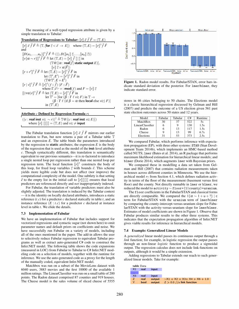
Figure 1. Radon model results. For Fabular/STAN, error bars in-dicate standard deviation of the posterior. For lmer/blmer, theyindicate standard error.

stores in 46 cities belonging to 50 chains. The Elections modelis a classic hierarchical regression discussed by Gelman and Hill(2007) and predicts the outcome of a US election given 561 paststate election outcomes across 50 states and 12 years.

Model Fabular Tabular C# RuntimeMatchBox 30 37 522 5s

LinearClassifier 6 9 130 1.5sRadon 6 13 117 1.5sCheese 9 13 99 6.7s

Elections 31 53 373 2.5s

We compared Fabular, which performs inference with expecta-tion propagation (EP), with three other systems: STAN (Stan Devel-opment Team 2014b), which implements an HMC-based methodcalled NUTS; lmer (Bates et al. 2014), an R package that performsmaximum likelihood estimation for hierarchical linear models; andblmer (Dorie 2014), which augments lmer with Bayesian priors.

We compared these in modelling a data set taken from Gel-man and Hill (2007) that contains radiation measurements takenin houses across different counties in Minnesota. We use the hier-archical model r7 from Section 4.1, which defines radiation activ-ity in terms of the floor of the measurement (basement versus firstfloor) and the county. Not directly runnable in lmer or blmer, wereduced the model to activity∼ floor+(1|county)+uranium.

The floor coefficients in the Fabular/STAN and classical formsare directly comparable. We compared the 1{α ∼ 1 + u+ ?} | cterm for Fabular/STAN with the uranium term of lmer/blmerby comparing the county-intercept-versus-uranium slope for Fabu-lar/STAN with the activity-versus-uranium slope for lmer/blmer.Estimates of model coefficients are shown in Figure 1. Observe thatFabular produces similar results to the other three systems. Thisindicates that the expectation propagation algorithm of Infer.NETgives viable results for inference in hierarchical models.

7.4 Example: Generalized Linear ModelsA generalized linear model passes its continuous output through alink function; for example, in logistic regression the output passesthrough an non-linear logistic function to produce a sigmoidaloutput. The regression calculus does not include link-functions onoutputs, although it would be a simple extension.

Adding regressions to Tabular extends our reach to such gener-alized linear models. Take for example:

table DataX1 real input...X6 real inputZ real output ∼X1 + X2 + X3+ X4 + X6 + 1.0Y bool output Z > 0.0 //a link function

280

Table Data consists of six real-valued clinical measurements X1trhough X6 and a Boolean label Y to be predicted (given some la-belled training points). This model is an instance of the Bayes PointMachine (Minka 2001), a boolean classifier, in which the prior overan implicit weight vector is drawn from a vector of Gaussian priors,and the label Y is generated by thresholding a latent score Z (theinner product of the weight and input vectors). (Intuitively, Z is thedistance of the point X1,..,X6 from the hyperplane defined by theweight vector; Z’s sign determines the side of the hyperplane occu-pied by the point). Here, the weight vector is implicitly defined bythe parameters of the regression; thresholding is the link function.(Gordon et al. 2015) describe a more verbose variant of this model.

7.5 Example: Latent Variable Mixture ModelFabular goes beyond traditional regression. Predictors are no longerrestricted to deterministic input data: they can be partially or evencompletely unobserved random variables. For example, considerthe task of regressing points belonging to a mixture of variouslines. If each point is labelled as belonging to a given class thenwe can use the label as the predictor that groups a family of linearregressions and infer the parameters of each line.

However, we can also generalize this model by assuming thatonly a subset of the points have been labelled. In Figure 2, weexplicitly impose a discrete distribution on each point’s Class. Thefigure contains both the Fabular code and its expansion to CoreTabular. The result is a supervised classifier, that infers the mostlikely class that each unlabelled point belongs to. (The operator |has lower precedence than + so the entire sum is grouped by Class.)

For example, here is a plot we generated using synthetic datafrom a mixture of three lines (training data points in light blue).

The blue, purple and green points are correctly classified, butthe red ones were incorrectly classified. The red points all lie closeto the intersections of the lines and are thus harder to separate.

If we furthermore assume that none of the points are labelled,then we obtain an unsupervised clustering algorithm, that partitionsthe points into three distinct sets of similar points.

7.6 Extension: Vectorized RegressionUntil now our predictors have had scalar types, but our notationextends naturally to vectorized regressions, whose predictors havevector types and contain arrays of scalars. The vectorized notationis convenient shorthand for the simultaneous definition of a fam-ily of regressions. Our Matchbox example, presented in the sequel,illustrates the feature. To generalize the notation, we index our re-gression judgments by the dimensionality d of the regression. Thescalar dimensionality • indicates a regression or predictor produc-ing a single scalar value (as before). The vector dimensionality •[n]indicates a regression or predictor producing an n-vector of scalarvalues. We also define the operation of dimensioning a type, writtend(T): •(T ) , T is just the identity on types while •[n](T ) , T [n],vectorizing its type argument.

Dimensionalities of Types:d ::= • | •[n] scalar or vector dimensionality

The typing rules for regressions are indexed by an additionaldimensionality d and enforce that the dimensions of subregressionsand coefficients are invariant and thus consistent.

Judgments of the Vectorized Type System:Γ;~e `d v : T d-dimensional predictor has type TΓ;~e;~f `d r ! Π d-dimensional regression r exports Π

Most rules merely propagate the invariant into sub-expressions.Rule (COEFF-VEC) generalizes rule (COEFF): it requires the typeof the predictor expression to match the expected dimension d andvectorizes the parameters α when d is a vector. Rule (SUM-VEC)restricts its terms to have the same dimensionality.

Typing Rules for Vectorized Regressions (extract):(COEFF-VEC)Γ;~e `d v : d(real) Γ;~f ; [] `d r ! Π α /∈ dom(Γ,Π)

Γ;~e;~f `d v{α ∼ r} ! (Π,α : d(real)[~f ])(SUM-VEC)Γ;~e;~f `d r ! Π (Γ,Π);~e;~f `d r′ ! Π′

Γ;~e;~f `d r+ r′ ! (Π,Π′)

Full typing judgments are presented in (Borgström et al. 2015).The details of the vectorizing translation are straightforward but

omitted for the sake of brevity. Constant predictors are replicated asvectors of constants; vectorized coefficient terms translate to vec-tors of component-wise products and sums of vectorized regres-sions translate to component-wise sums of vectors.

In our Fabular implementation, the decision to vectorize a re-gression is driven by the type of the attribute defined by that re-gression. For added convenience, scalar predictors appearing in acontext expecting a vector are implicitly cast into the appropriatelysized vector (by replication).

7.7 Example: MatchboxMatchbox (Stern et al. 2009) is a recommender system that worksby integrating metadata about users and items. The system repre-sents users and items as trait vectors in a common latent space anddefines the affinity between users and items as the dot product oftheir vectors. Matchbox then uses this affinity to predict the rat-ings that a user would give to an item. We demonstrate that, to oursurprise, this matrix model of recommendations can be conciselycaptured as a Fabular vectorized regression.

In Matchbox, u ∈ Rn and m ∈ Rm are sparse binary vectorsrepresenting metadata for users and items, respectively. For illus-tration, we might have n = 3 users and m = 2 movies as items:

u =

userId0 0userId1 0userId2 1

m =

(movieId0 1movieId1 0

)Thus, rows are labelled by values for dimensions of the meta-

data, e.g., u has one row per user id, while m has one row permovie id. We project u and m into a common trait space by left-multiplying them by random matrices UT and MT , which have di-mensions k×n and k×m, yielding ut = UTu and mt = MTm, e.g.,for k = 2 and trait space R2:

ut =(

UT00 UT01 UT02UT10 UT11 UT12

)×

001

=

(UT02UT12

)Where the individual UTi j and MTi j components are drawn fromindependent Gaussians (note that we sample a single UT and MT

281

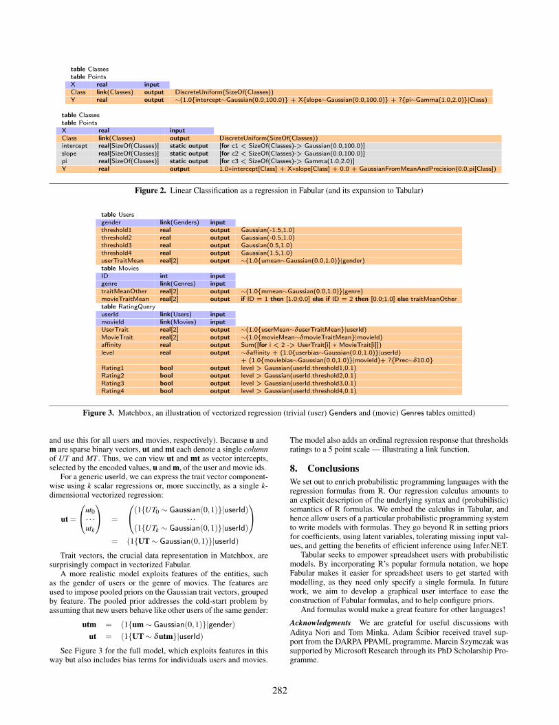
table Classestable PointsX real inputClass link(Classes) output DiscreteUniform(SizeOf(Classes))Y real output ∼(1.0{intercept∼Gaussian(0.0,100.0)} + X{slope∼Gaussian(0.0,100.0)} + ?{pi∼Gamma(1.0,2.0)}|Class)

table Classestable PointsX real inputClass link(Classes) output DiscreteUniform(SizeOf(Classes))intercept real[SizeOf(Classes)] static output [for c1 < SizeOf(Classes)-> Gaussian(0.0,100.0)]slope real[SizeOf(Classes)] static output [for c2 < SizeOf(Classes)-> Gaussian(0.0,100.0)]pi real[SizeOf(Classes)] static output [for c3 < SizeOf(Classes)-> Gamma(1.0,2.0)]Y real output 1.0∗intercept[Class] + X∗slope[Class] + 0.0 + GaussianFromMeanAndPrecision(0.0,pi[Class])

Figure 2. Linear Classification as a regression in Fabular (and its expansion to Tabular)

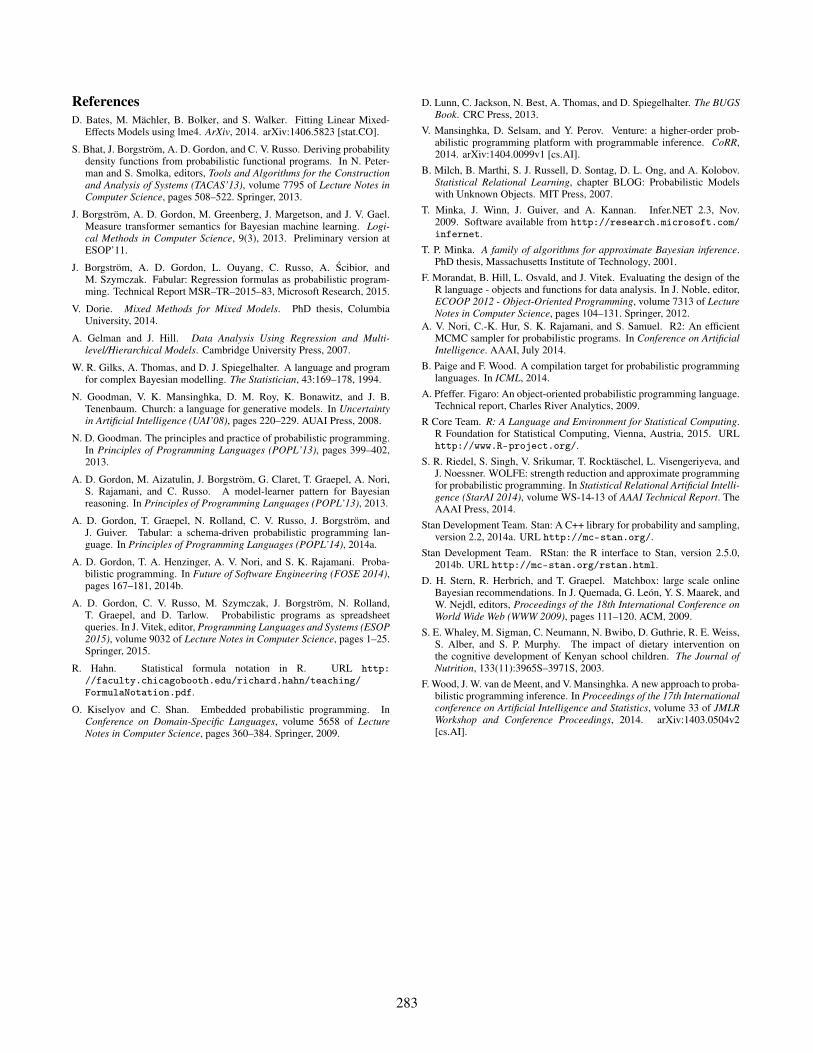
table Usersgender link(Genders) inputthreshold1 real output Gaussian(-1.5,1.0)threshold2 real output Gaussian(-0.5,1.0)threshold3 real output Gaussian(0.5,1.0)threshold4 real output Gaussian(1.5,1.0)userTraitMean real[2] output ∼(1.0{umean∼Gaussian(0.0,1.0)}|gender)table MoviesID int inputgenre link(Genres) inputtraitMeanOther real[2] output ∼(1.0{mmean∼Gaussian(0.0,1.0)}|genre)movieTraitMean real[2] output if ID = 1 then [1.0;0.0] else if ID = 2 then [0.0;1.0] else traitMeanOthertable RatingQueryuserId link(Users) inputmovieId link(Movies) inputUserTrait real[2] output ∼(1.0{userMean∼δuserTraitMean}|userId)MovieTrait real[2] output ∼(1.0{movieMean∼δmovieTraitMean}|movieId)affinity real output Sum([for i < 2 -> UserTrait[i] ∗ MovieTrait[i]])level real output ∼δaffinity + (1.0{userbias∼Gaussian(0.0,1.0)}|userId)

+ (1.0{moviebias∼Gaussian(0.0,1.0)}|movieId)+ ?{Prec∼δ10.0}Rating1 bool output level > Gaussian(userId.threshold1,0.1)Rating2 bool output level > Gaussian(userId.threshold2,0.1)Rating3 bool output level > Gaussian(userId.threshold3,0.1)Rating4 bool output level > Gaussian(userId.threshold4,0.1)

Figure 3. Matchbox, an illustration of vectorized regression (trivial (user) Genders and (movie) Genres tables omitted)

and use this for all users and movies, respectively). Because u andm are sparse binary vectors, ut and mt each denote a single columnof UT and MT . Thus, we can view ut and mt as vector intercepts,selected by the encoded values, u and m, of the user and movie ids.

For a generic userId, we can express the trait vector component-wise using k scalar regressions or, more succinctly, as a single k-dimensional vectorized regression:

ut =

ut0· · ·utk

=

(1{UT0 ∼ Gaussian(0,1)}|userId)· · ·

(1{UTk ∼ Gaussian(0,1)}|userId)

= (1{UT∼ Gaussian(0,1)}|userId)

Trait vectors, the crucial data representation in Matchbox, aresurprisingly compact in vectorized Fabular.

A more realistic model exploits features of the entities, suchas the gender of users or the genre of movies. The features areused to impose pooled priors on the Gaussian trait vectors, groupedby feature. The pooled prior addresses the cold-start problem byassuming that new users behave like other users of the same gender:

utm = (1{um∼ Gaussian(0,1)}|gender)ut = (1{UT∼ δutm}|userId)

See Figure 3 for the full model, which exploits features in thisway but also includes bias terms for individuals users and movies.

The model also adds an ordinal regression response that thresholdsratings to a 5 point scale — illustrating a link function.

8. ConclusionsWe set out to enrich probabilistic programming languages with theregression formulas from R. Our regression calculus amounts toan explicit description of the underlying syntax and (probabilistic)semantics of R formulas. We embed the calculus in Tabular, andhence allow users of a particular probabilistic programming systemto write models with formulas. They go beyond R in setting priorsfor coefficients, using latent variables, tolerating missing input val-ues, and getting the benefits of efficient inference using Infer.NET.

Tabular seeks to empower spreadsheet users with probabilisticmodels. By incorporating R’s popular formula notation, we hopeFabular makes it easier for spreadsheet users to get started withmodelling, as they need only specify a single formula. In futurework, we aim to develop a graphical user interface to ease theconstruction of Fabular formulas, and to help configure priors.

And formulas would make a great feature for other languages!

Acknowledgments We are grateful for useful discussions withAditya Nori and Tom Minka. Adam Scibior received travel sup-port from the DARPA PPAML programme. Marcin Szymczak wassupported by Microsoft Research through its PhD Scholarship Pro-gramme.

282

ReferencesD. Bates, M. Mächler, B. Bolker, and S. Walker. Fitting Linear Mixed-

Effects Models using lme4. ArXiv, 2014. arXiv:1406.5823 [stat.CO].

S. Bhat, J. Borgström, A. D. Gordon, and C. V. Russo. Deriving probabilitydensity functions from probabilistic functional programs. In N. Peter-man and S. Smolka, editors, Tools and Algorithms for the Constructionand Analysis of Systems (TACAS’13), volume 7795 of Lecture Notes inComputer Science, pages 508–522. Springer, 2013.

J. Borgström, A. D. Gordon, M. Greenberg, J. Margetson, and J. V. Gael.Measure transformer semantics for Bayesian machine learning. Logi-cal Methods in Computer Science, 9(3), 2013. Preliminary version atESOP’11.

J. Borgström, A. D. Gordon, L. Ouyang, C. Russo, A. Scibior, andM. Szymczak. Fabular: Regression formulas as probabilistic program-ming. Technical Report MSR–TR–2015–83, Microsoft Research, 2015.

V. Dorie. Mixed Methods for Mixed Models. PhD thesis, ColumbiaUniversity, 2014.

A. Gelman and J. Hill. Data Analysis Using Regression and Multi-level/Hierarchical Models. Cambridge University Press, 2007.

W. R. Gilks, A. Thomas, and D. J. Spiegelhalter. A language and programfor complex Bayesian modelling. The Statistician, 43:169–178, 1994.

N. Goodman, V. K. Mansinghka, D. M. Roy, K. Bonawitz, and J. B.Tenenbaum. Church: a language for generative models. In Uncertaintyin Artificial Intelligence (UAI’08), pages 220–229. AUAI Press, 2008.

N. D. Goodman. The principles and practice of probabilistic programming.In Principles of Programming Languages (POPL’13), pages 399–402,2013.

A. D. Gordon, M. Aizatulin, J. Borgström, G. Claret, T. Graepel, A. Nori,S. Rajamani, and C. Russo. A model-learner pattern for Bayesianreasoning. In Principles of Programming Languages (POPL’13), 2013.

A. D. Gordon, T. Graepel, N. Rolland, C. V. Russo, J. Borgström, andJ. Guiver. Tabular: a schema-driven probabilistic programming lan-guage. In Principles of Programming Languages (POPL’14), 2014a.

A. D. Gordon, T. A. Henzinger, A. V. Nori, and S. K. Rajamani. Proba-bilistic programming. In Future of Software Engineering (FOSE 2014),pages 167–181, 2014b.

A. D. Gordon, C. V. Russo, M. Szymczak, J. Borgström, N. Rolland,T. Graepel, and D. Tarlow. Probabilistic programs as spreadsheetqueries. In J. Vitek, editor, Programming Languages and Systems (ESOP2015), volume 9032 of Lecture Notes in Computer Science, pages 1–25.Springer, 2015.

R. Hahn. Statistical formula notation in R. URL http://faculty.chicagobooth.edu/richard.hahn/teaching/FormulaNotation.pdf.

O. Kiselyov and C. Shan. Embedded probabilistic programming. InConference on Domain-Specific Languages, volume 5658 of LectureNotes in Computer Science, pages 360–384. Springer, 2009.

D. Lunn, C. Jackson, N. Best, A. Thomas, and D. Spiegelhalter. The BUGSBook. CRC Press, 2013.

V. Mansinghka, D. Selsam, and Y. Perov. Venture: a higher-order prob-abilistic programming platform with programmable inference. CoRR,2014. arXiv:1404.0099v1 [cs.AI].

B. Milch, B. Marthi, S. J. Russell, D. Sontag, D. L. Ong, and A. Kolobov.Statistical Relational Learning, chapter BLOG: Probabilistic Modelswith Unknown Objects. MIT Press, 2007.

T. Minka, J. Winn, J. Guiver, and A. Kannan. Infer.NET 2.3, Nov.2009. Software available from http://research.microsoft.com/infernet.

T. P. Minka. A family of algorithms for approximate Bayesian inference.PhD thesis, Massachusetts Institute of Technology, 2001.

F. Morandat, B. Hill, L. Osvald, and J. Vitek. Evaluating the design of theR language - objects and functions for data analysis. In J. Noble, editor,ECOOP 2012 - Object-Oriented Programming, volume 7313 of LectureNotes in Computer Science, pages 104–131. Springer, 2012.

A. V. Nori, C.-K. Hur, S. K. Rajamani, and S. Samuel. R2: An efficientMCMC sampler for probabilistic programs. In Conference on ArtificialIntelligence. AAAI, July 2014.

B. Paige and F. Wood. A compilation target for probabilistic programminglanguages. In ICML, 2014.

A. Pfeffer. Figaro: An object-oriented probabilistic programming language.Technical report, Charles River Analytics, 2009.

R Core Team. R: A Language and Environment for Statistical Computing.R Foundation for Statistical Computing, Vienna, Austria, 2015. URLhttp://www.R-project.org/.

S. R. Riedel, S. Singh, V. Srikumar, T. Rocktäschel, L. Visengeriyeva, andJ. Noessner. WOLFE: strength reduction and approximate programmingfor probabilistic programming. In Statistical Relational Artificial Intelli-gence (StarAI 2014), volume WS-14-13 of AAAI Technical Report. TheAAAI Press, 2014.

Stan Development Team. Stan: A C++ library for probability and sampling,version 2.2, 2014a. URL http://mc-stan.org/.

Stan Development Team. RStan: the R interface to Stan, version 2.5.0,2014b. URL http://mc-stan.org/rstan.html.

D. H. Stern, R. Herbrich, and T. Graepel. Matchbox: large scale onlineBayesian recommendations. In J. Quemada, G. León, Y. S. Maarek, andW. Nejdl, editors, Proceedings of the 18th International Conference onWorld Wide Web (WWW 2009), pages 111–120. ACM, 2009.

S. E. Whaley, M. Sigman, C. Neumann, N. Bwibo, D. Guthrie, R. E. Weiss,S. Alber, and S. P. Murphy. The impact of dietary intervention onthe cognitive development of Kenyan school children. The Journal ofNutrition, 133(11):3965S–3971S, 2003.

F. Wood, J. W. van de Meent, and V. Mansinghka. A new approach to proba-bilistic programming inference. In Proceedings of the 17th Internationalconference on Artificial Intelligence and Statistics, volume 33 of JMLRWorkshop and Conference Proceedings, 2014. arXiv:1403.0504v2[cs.AI].

283