Embed Size (px)
Citation preview

Fabian Kühnhausen:
Financial Innovation and Fragility
Munich Discussion Paper No. 2014-37
Department of EconomicsUniversity of Munich
Volkswirtschaftliche FakultätLudwig-Maximilians-Universität München
Online at http://epub.ub.uni-muenchen.de/21173/

Electronic copy available at: http://ssrn.com/abstract=2404881
Financial Innovation and Fragility∗
Fabian Kuhnhausen†
Juni 23, 2014
Abstract
In this paper, I evaluate the impact of innovative activity of financialagents on their fragility in a competitive framework. There exist a vastarray of concerns about the interconnection of financial innovations,financial distress of firms and financial crises provided by theoreticalarguments. I build on these and assess empirically the causal link be-tween a financial agents’ innovativeness and stability.Using a unique data set on financial innovations in the USA between1990 and 2002, I show that a larger degree of innovation negatively(positively) affects firm stability (fragility) after controlling for the un-derlying firm characteristics. The results are robust against differentmodifications of innovation measures and against different fragility pa-rameters indicating profitability, activity risk and risk of insolvency.
JEL Codes: G01, G2, L11, O31Keywords: Incentives to Innovate, Financial Innovation, Fragility
∗Helpful comments were provided by participants at the Annual Meeting of the EasternFinance Association in 2014, the Royal Economic Society PhD Meeting 2014, the ThirdWorkshop ”Banking and Financial Markets”, the MPI-ZEW Workshop on Law & Eco-nomics, the Borsa Istanbul Finance and Economics Conference 2013 and the ETH/IMPRS-CI Workshop on Law & Economics as well as by seminar participants at the Max PlanckInstitute for Innovation and Competition and Ludwig Maximilian University of Munich.This paper received the Outstanding Doctoral Student Paper Award from the EasternFinance Association. An earlier version of this work entitled ”The Impact of FinancialInnovation on Firm Stability” was published in the BIFEC 2013 Proceedings. Finan-cial support by the Max Planck Institute for Innovation and Competition is gratefullyacknowledged.†Doctoral Fellow at the International Max Planck Research School for Competition and
Innovation (IMPRS-CI) and PhD candidate at Ludwig Maximilian University of Munich.Contact address: Max Planck Institute for Innovation and Competition, Marstallplatz 1,80539 Munich, Germany, email: [email protected].

Electronic copy available at: http://ssrn.com/abstract=2404881
1 Introduction
Numerous researchers have analyzed the causes for distress of financial
agents during the recent financial crisis starting in 2007. Through both theo-
retical and empirical analyses, they came up with a variety of reasons. These
include panics of bank customers and major investors, shocks to money sup-
ply, debt financing and to the real economy, as well as the interconnectedness
of banks and their complexity. A recent strand of literature1 tries to argue,
however, that a competitive financial system and the non-patentability of
financial innovations (FI) can cause a financial crisis. These papers analyze
the incentives to innovate and the relation to financial distress. Despite the
plentiful theoretical literature, only a few empirical studies on that relation
exist. These have provided evidence on the drivers for product development
and competition in financial markets. This work provides additional insight
into the empirical relationship between innovation and stability in financial
markets.
In this paper, I follow the innovation-fragility view2 and explore whether
more innovative financial systems are more prone to financial crises. To do
so, I analyze the proposed causal and positive relationship between FI and
incidents of a financial distress in an empirical setup with US data on the
agent level. The precipitating question is who innovates in the financial mar-
ket? Is the degree of innovativeness positively related to an agent’s profit
volatility? Does innovative activity increase the risk of insolvency? In other
words, is competition through innovation negatively related to stability?
1Starting with Bhattacharyya/Nanda (2000). A more detailed literature review is givenin Section 2. This also provides the theoretical underpinnings for the empirical analysesin Section 3.
2See Beck et al. (2012).
1

I utilize count data and patents to measure FI on a micro level from Lerner
(2006) and relate agent-level variations in innovativeness to profit volatility
of financial institutions while controlling for firm characteristics and time
trends. Based on an empiral setup that corresponds to Hasan et al. (2009),
Demirguc-Kunt and Huizinga (2010), Beck et al. (2012), and Lepetit and
Strobel (2012), I investigate the link between profit volatility and FI in a
dynamic panel model. I find a significant positive relation which implies
a negative impact on the stability of the financial system. Furthermore, I
check my results against a number of different extensions. While regressions
with interactions between firm characteristics and FI provide ambiguous
results, my findings are confirmed with different innovation measures and
different fragility measures. In addition, more innovative firms face higher
losses during a period of crisis.
The paper is structured as follows. First, I discuss previous literature in
the area. In Section 3 I introduce the data while in Section 4 I present
the empirical analysis. In Section 5 I discuss the results, while Section 6
concludes the paper and suggests topics for future research.
2

2 Literature Review
This paper draws on literature from two distinct research areas: (i) micro-
and macroeconomic research on the existence of financial crises and (ii)
investigations into the foundations of FI.3
2.1 Financial Crises
The first field of research pertains to the origins and persistence of financial
crises, or more particularly, the investigation of causes for financial distress
of single agents providing any kind of financial services. In their seminal
paper, Allen and Gale (2000) investigate possible contagion and bubbles in
financial networks. They build a model of contagion with perfectly compet-
itive banking and show that a first-best allocation of risk-sharing is possible,
but fragility still persists. Subsequently, Upper and Worms (2004) confirm
Allen and Gale’s (2000) model by empirically evaluating the risk of conta-
gion and credit risk in the German interbank lending market.4 Their analysis
provides two results: First, credit risk may trigger a domino effect in that
there exists considerable scope for contagion even with safety mechanisms.
Second, more concentrated structures can lower the threshold for contagion.5
Furthermore, Allen and Gale (2004) analyze the relation between compe-
tition and financial stability. Here, they find a negative trade-off between
both while considering a variety of different settings such as general equi-
3General surveys about research on financial agents with particular focus on asymmetriesof information and security design are given by Allen and Winton (1995) and Duffie andRahie (1995).
4They use balance sheet data of German banks to estimate bilateral credit relationships.5Many more papers can be found which empirically analyze the causes for financial crisesboth at a micro- and macro-level. Since I want to focus on the distinct relationshipbetween FI and financial health, an extended overview on that area of literature wouldbe beyond the scope of this paper.
3

librium models, agency models, Schumpeterian competition and contagion.
In a three-period model with risky and standard assets as well as timing
incongruity, they show that greater competition is good for efficiency, but
bad for financial stability. Additionally, Allen et al. (2009) provide a thor-
ough review on financial crises. They find that most financial crises arise
from panics, business cycle fluctuations or contagion, and derive from this
evidence a common sequence of events.6
2.2 Financial Innovations
A second strand of literature looks at the origins and existence of financial
innovations.7 The seminal definition of FI is given by Tufano (2003): It
is the creation of financial instruments (both product and process) by in-
vention or diffusion of products, services or ideas. He states that FI exists
because of the incompleteness of markets, for managing risk, for pooling
of funds and because of regulation. Frank and White (2004, 2009) review
the technological changes and innovations in commercial banking over the
last 25 years. They employ the same definition of FI as Tufano (2003) and
argue that FI reduce costs and risks, pool funds and provide a tool to serve
demands of investors. In addition, they survey the literature to illustrate
innovation patterns over the investigated period.
From a theoretical perspective, numerous papers provide arguments for the
existence of innovations in financial markets. Most recently, Michalopoulos
6With surging money supply, asset prices and credit volumes increase which inevitably leadto a price bubble bound to burst. A banking crisis is then followed by an exchange-ratecrisis and a substantial drop in real output. Brunnermeier (2009) presents an overviewon the development of the recent financial crisis and uses micro- and macro-level data tosuggest reasonable policy interventions.
7Tufano (2003), Frank and White (2004, 2009) as well as Lerner and Tufano (2011) provideoverviews on innovations in the financial market.
4

et al. (2011) link FI to the endogeneous growth theory while Carvajal et
al. (2012) examine innovations in frictionless financial markets with short
selling. They find incomplete markets even with costless innovation and
competition. Ferreira et al. (2012) argue that the form of equity financing
determines FI incentives. In their model, they suggest to go public for ex-
ploiting existing ideas and go private for exploring new, risky ideas. Song
and Thakor (2010) and Shen et al. (2012) provide arguments for collateral-
motivated FI and link possible innovation cycles in financial markets to
government regulation such as Basel III.
Empirical assessments of innovations in financial markets have started with
research in the 1980s and 1990s.8 In his early contribution, Tufano (1989)
argues that FI provide first-mover advantages. He assesses the dynamics of
innovations and competition by analyzing data on 58 publicly offered FI in
the years 1974 to 1987 which raised USD 280 billion and providing cross-
sectional regressions of the underwriting spread on firm characteristics.9 He
finds that 20% of new securities being issued in 1987 have not been in exis-
tence in 1974 and that new product ideas diffuse rapidly across competitors
so that banks do not enjoy monopoly pricing with innovations, but rather
capture a larger market share with lower prices than their imitators.
Lerner (2002) looks at financial patents during the period 1971 to 2000
and analyzes the impact of the State Street decision10 on the degree of inno-
8See e.g. Miller (1986, 1992), Merton (1992), Frank and White (2004, 2009).9Tufano (1989) relied on three data sources: first, a literature search using ABI-Inform andBusiness Periodical Index; second, interviews with investment bankers; third, companydata from SDC and IDDIS.
10State Street Bank vs. Signature Financial Group was a 1998 decision by the US Court ofAppeals for the Federal Circuit (CAFC) regarding the patentability of business methods.Herein, the CAFC rejected the notion of a business method exception and allowed theprotection of an invention if it involved some practical application and some tangible
5

vation observable in the market. He uses the classification of the US Patent
and Trademark Office and the Delphion IP Network to identify 445 financial
patents and finds a surge in patenting filed mostly by large corporations. In
addition, Lerner (2006) investigates the origins of innovations by developing
a new measure for FI. His regressions show that small, less profitable firms
are more innovative with an additional agglomeration effect. More recently,
Lerner (2010) inquires about litigation of patents on FI.11 He analyzes fi-
nancial patent awards by the US Patent and Trademark Office between 1976
and 2003 in combination with firm-level data from public records. He finds
that first, patents on FI are litigated more often than normal patents; sec-
ond, litigated patents are mostly owned by small firms or individuals and
have more claims and citations than other financial patents; and third, large
firms are more often defendants in litigation.
Finally, Boz and Mendoza (2010) examine the interaction of FI, learning
and collateral constraints in a stochastic equilibrium model of household
debt and land prices. They use an experimental setup with switching be-
tween high- and low-leverage regimes according to Bayesian learning and
find that innovations in financial markets lead to boom-bust cycles.
The financial innovations considered in this paper differ from innovations
in product markets in several important ways. In general, consumers of fi-
nancial services face opacity about the portfolio of financial agents and their
quality provided in financial services. Also, research has not yet produced
result, which with regards to financial patents was deemed the pricing. However, the2008 CAFC decision In re Bilski rejected the tangible result test as inadequate. TheUS Supreme Court affirmed this judgement in Bilski vs. Kappos. This leaves companieswith great uncertainty over the patentability of financial innovations.
11This again draws on Lerner (2002).
6
any structural model with which to estimate both supply and demand of
FI. Frank and White (2004) survey empirical studies on FI and point to
the general scarcity in research in that field. Lerner and Tufano (2011) also
show some differences between FI and manufacturing innovations, most no-
tably stressing different dynamics and agency structures. They point out
the problems of assessing FI due to the rarity of R&D spending by financial
agents, the infrequency or non-existence of financial patents and the opacity
of FI by private firms.
2.3 Incentives to Innovate and Financial Crises
This paper makes use of a new strand of literature combining both afore-
mentioned research fields. Most work focuses on the innovation-fragility
view coined by Beck et al. (2012) that innovations may have adverse ef-
fects on competition and stability. It begins with early theoretical work
by Bhattacharyya and Nanda (2000). Their paper is the first to connect
incentives to innovate and the analysis of financial crises in a theoretical
setup. Because client characteristics, market structure and the volatility
affect switching costs and costs of delayed adoption, banks with greater
market power and more secure relationships with customers are more likely
to innovate. Empirical assessments of the causal link between innovations
and financial instability have been scarce.
Most recently, two lines of argumentation have emerged. The first one fo-
cuses on incentive structures and volatility in financial markets. Thakor
(2012) analyzes the relation between incentives to innovate and financial
crises. He makes use of Allen and Gale’s (2004) model with three periods
where the distinction is not between standard and risky assets, but now
7

between standard and innovative assets. Financial agents then face the
trade-off between making profits from innovation and refinancing risks. In
his model, the degree of innovativeness is positively related to the refinanc-
ing risk which makes imitation less likely and drives up profits. Reasons
for financial distress are then the competitive financial system and the non-
patentability of FI because of the correlation of default risks if FI can be
imitated.
Beck et al. (2012) evaluate the respective relationships between FI and real
sector growth, real sector volatility and bank fragility using bank-, industry-
and country-level data from 32 countries during the period 1996 to 2006.
Approximating Tufano’s (2003) definition of FI by financial R&D intensity
obtained from the OECD, they analyze the innovation-fragility view on FI.
Namely, they relate country-level variation in FI to bank-level variation in
profits and volatility. Their results show that innovativeness leads to in-
creasing fragility, risk taking, profit volatility and bank losses during crises.
Herein, smaller, fast growing banks are more fragile in countries with more
FI while smaller, less leveraged banks are more effected by agglomeration
effects.
A second line of argumentation focuses on investors’ behavior. Shleifer and
Vishny (2010) set up a behavioral finance model where they assume opti-
mism of investors as stimulus for demand for new securities and pessimism
as a shock leading to financial crises. Mispricing occurs because financial
agents profit from investors’ misperceptions. Depressed securities then have
adverse welfare effects ex post as they cut off lending to new instruments.
Overall, securitization raises the level of investment and cyclicality. Hender-
8

son and Pearson (2011) show that investors can be exploited by innovative
financial products. Their event study proposes that issuers innovate to sell
new securities at a risk-adjusted premium to uninformed investors because
innovativeness increases complexity and ambiguity. Subsequently, issuers
exploit investors’ misunderstandings of financial market. The authors pro-
vide reasons for excess demand in overconfidence, framing and loss aversion
of investors.
Jeon and Nishihara (2012) extend Shleifer and Vishny’s (2010) model and
allow agents to securitize risky assets with leverage and asymmetric infor-
mation. They find that risk retention requirements imposed by governments
reduce welfare. Concurrently, Gennaioli et al. (2012) argue that FI cause
crises because of neglected risks. Their research is also an extension of the
Shleifer and Vishny (2010) paper whereby agents engineer securities per-
ceived to be safe but exposed to neglected risks which leads to excessive
security issuance. They apply a model of belief formation to relate FI, se-
curity issuance, risk perception and financial fragility.
This paper follows the recent strand of new literature on the relationship be-
tween incentives to innovate and financial instability. The paper’s contribu-
tion is the empirical connection between financial innovations and instability
of financial agents. There exist only a few empirical analyses focusing either
on particular innovations (Henderson and Pearson 2011) or on cross-country
comparisons (Beck et al. 2012) so far. To the best of my knowledge this
paper is the first quantitative assessment of the innovation-fragility view at
the agent level. I employ a data set by Lerner (2006) and augment it with
performance and stability measures so that I can study the effect of firm-
9

level variation in FI on the stability of financial agents. Although I focus
here on the USA, this firm-level analysis can offer insights into the incentives
to innovate and dynamics in a competitive financial system.
3 Data
The data set measures financial innovations in the USA from 1990 until 2002
via a unique counting mechanism.12 Lerner (2006) investigates the origins
of innovations and develops a new FI measure based on news stories from
the Wall Street Journal during the period 1990 to 2002 which he merges
with additional information from the SEC, Compustat, finance journals and
the US Patent and Trademark Office to establish a link between innovative
ability, firm characteristics and patenting.13 The sample consists of firms
with either at least one innovation observed by the measure during the time
period or being active in the SIC codes 60 through 64 and 67.14
The data set consists of four different groups of variables:15 First, I use
firm characteristics to control for firm-specific effects. In accordance with
Lerner (2006), I use the logarithm of total assets to measure firm size. Prof-
itability (Opprof) is defined as earnings before interest, taxes, depreciation
and amortization (EBITDA) divided by revenues, and leverage is defined
as the ratio of the book value of a firm’s long-term debt to total capitaliza-
tion. Further control variables include firm age, cash equivalents, employees,
shareholders’ equity, long-term debt, common market value and revenues.
12The data were kindly provided by Josh Lerner, Harvard Business School.13See also Lerner (2002) for his aforementioned earlier work on financial patents.14These SIC codes include firms operating in the financial services business such as insur-
ance, banking, financial advisory and so on except for real estate.15For complete descriptions of the variables used here, see Table A1 in the Appendix.
10

Second, the data set includes performance measures like EBITDA, net in-
come, retained earnings as well as return on assets (ROA) and return on
equity (ROE) which are used to derive the stability measures and provide
information about the competitive nature.
Third, I measure stability of financial institutions with the Z-score. The Z-
score is a measure of bank solvency and corresponds to (ROA+CAR)/σ(ROA).
It ”indicates the number of standard deviations that a bank’s rate of return
on assets can fall in a single period before it becomes insolvent. A higher
Z-score signals a lower probability of bank insolvency” (Beck et al. 2012).16
For robustness checks, I later also use other stability measures such as the
capital-asset ratio (CAR), standard deviations of returns, and the Sharpe
ratio which is defined as ROE/σ(ROE).
Fourth, innovation is measured by the count of patent applications, patents
issued and stories on innovations per year and firm. I also include a measure
for the agglomeration effect by counting the number of innovations by other
firms within the same two-digit ZIP code area as a firm.
All financial data is in million 2002 US Dollars. Financial and company
data comes directly from Compustat or is calculated from its pool of vari-
ables. The count data on innovations comes from articles issued in the Wall
Street Journal or the Factiva database on technological inventions. Patent
data comes from the US Patent and Trademark Office. For a comprehensive
explanation of the data set, see Lerner (2006). I clean the data from coding
16See Lepetit and Strobel (2013) for more information on firm’s insolvency risk and dif-ferent approaches to time-varying Z-score measures. They provide a derivation of theZ-score and discuss several ways to estimate means and standard deviations of the vari-ables used to calculate the measure. I follow their recommended specification.
11

errors and outliers, and perform some plausibility checks. Any observations
with implausible values for balance sheet items (e.g. negative revenues) are
dropped. I also exclude observations with negative Z-scores. The final sam-
ple is an unbalanced panel with 19,895 firm-year observations of 3,042 firms.
Like any other measure of FI, the count measure used here also has its lim-
itations. It necessarily excludes private firms not listed in Compustat. Fur-
thermore, the time period is rather limited and the methodology to source
the counts of innovations from the articles is based on stylized facts of FI.
Also, problems in assessing FI exist due to the rarity of R&D spending by
financial institutions, the infrequency of financial patents and the intrans-
parency of FI by private firms as discussed by Tufano (2003), Frank and
White (2004, 2009) and Lerner and Tufano (2011). Therefore, the count
measure introduced by Lerner (2006) and applied here to analyze finan-
cial fragility is a promising first start to assess empirically the connection
between financial innovations and instability of financial agents.
12

4 Empirical Analysis
This section explores the relationship between FI and financial agents’ fragility
empirically. I first provide a description of the data and then present the
empirical model specification.
4.1 Descriptive Statistics and Properties
Table 1 provides an overview of the summary statistics of the variables. It
shows that there exists great heterogeneity among firms in terms of size and
profitability. Because I include all firms active in financial services, leverage
ratios are comparably low. Stability measures are constructed from the firm
characteristics to capture a firm’s insolvency risk and activity risk. Higher
numbers for the Sharpe ratio and the Z-score reflect less fragility. Moreover,
the count data on FI includes a lot of zeros as indicated by the low means.17
Generally, variances of the variables are quite large. For most variables,
mean values are larger than the median because there are a lot of firms in
the sample whose observations depict values close to zero for the variables
used here.
Observations are evenly distributed over the time period and firm char-
acteristics exhibit a high degree of persistence. About 11% of firms in the
sample have observations for the entire time period. About 26% of firms
have 8 or more consecutive observations. On average, the data set has 9
observations per firm.
17In total, the data set includes only 588 incidences of financial innovation.
13

Table 1: Summary Statistics of Key Variables
Variable Mean Median Std. Dev. Min. Max.
Age 9.550 6.000 11.971 0 77Assets 12806.760 604.177 57441.090 0 1097190Cash Equiv. 1348.839 28.258 8608.241 0 316206Leverage 0.278 0.213 0.263 0 0.999Long-term Debt 1698.329 36.057 11639.600 0 468570Market Value 2939.847 138.685 15583.860 0 535947Pref. Stock 38.948 0.000 223.152 0 5712Revenues 2607.716 78.583 11729.980 0 186857Sh. Equity 1306.896 91.860 5115.215 -515.745 153738
Opprof 0.077 0.291 6.850 -587.544 19.483Ret. Earnings 776.869 24.195 3527.743 -15801 81210ROA 0.050 0.011 1.723 -16.444 235.667ROE 0.835 0.104 49.136 -125.869 4787.999
CAR 0.226 0.127 3.231 -441 3.414HHI 0.014 0.014 0.002 0.011 0.019σ(ROA) 0.142 0.008 4.875 0 650.898σ(ROE) 1.557 0.046 45.011 0 2194.872Sharpe 3.702 2.211 8.642 -103.399 346.778Z-score 42.926 22.897 194.269 0 12381.450
Innovations 0.016 0.000 0.165 0 6Patents 0.033 0.000 0.416 0 15Applications 0.031 0.000 0.432 0 21R&D 45.594 0.000 436.137 0 9845FI by Others 2.442 0.000 3.441 0 12
Notes: N=19,895. The list is ordered according to the four different groupsof variables mentioned above. See Table A1 in the Appendix for definitions ofthe variables. All financial data is in million 2002 US Dollars and comes fromCompustat. Count data on innovations comes from the Wall Street Journal,the Factiva database or the US Patent and Trademark Office, collected byLerner (2006).
Figure 1 displays firm characteristics over time. There exists a general in-
crease in the absolute values of these firm-specific variables. Similar to
Figure 1, Figure 2 presents the evolution of a firm’s performance and sta-
bility measures over the time period. There is no clear trend in rising or
falling profitability of financial institutions. While retained earnings and the
Sharpe ratio increase over time, operational profitability, the capital-asset
14

ratio and returns on assets and equity decline.
Figure 1: Firm Characteristics
010
0020
0030
0040
0050
00O
ther
Indi
cato
rs (
in m
n U
SD
)
5000
1000
015
000
2000
0A
sset
s (in
mn
US
D)
1990 1991 1992 1993 1994 1995 1996 1997 1998 1999 2000 2001 2002
Total Assets Cash Equiv. Long-term Debt
Common Market Value Preferred Stock Revenues
Shareholders' Equity
Figure 2: Profitability and Stability Measures
500
600
700
800
900
1000
Ret
aine
d E
arni
ngs
(in m
n U
SD
)
01
23
4R
atio
s
1990 1991 1992 1993 1994 1995 1996 1997 1998 1999 2000 2001 2002
Capital-asset Ratio Sharpe Ratio EBITDA/Revenues
ROA ROE Ret. Earnings
Figure 3 presents how the count of FI has developed over time. The notable
peak towards the late 1990s is due to the aforementioned State Street deci-
sion. Observations for patents lag behind applications because the average
time period between applying for a patent and granting patents is about two
to three years. Only applications for patents granted during the time period
are included in the data set. Overall, the number of observed innovations
is rather low in comparison to the overall size of the data set so that this is
one point of caution.
Figure 4 presents a comparison of fragility by grouping firms with measured
15
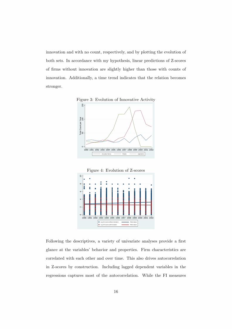
innovation and with no count, respectively, and by plotting the evolution of
both sets. In accordance with my hypothesis, linear predictions of Z-scores
of firms without innovation are slightly higher than those with counts of
innovation. Additionally, a time trend indicates that the relation becomes
stronger.
Figure 3: Evolution of Innovative Activity
050
100
150
Tot
al C
ount
per
Yea
r
1990 1991 1992 1993 1994 1995 1996 1997 1998 1999 2000 2001 2002
Innovation Stories Patents Applications
Figure 4: Evolution of Z-scores
02
46
810
1990 1991 1992 1993 1994 1995 1996 1997 1998 1999 2000 2001 2002
Log of Z-scores without innovation
Log of Z-scores with Innovation
Fitted values
Fitted values
Following the descriptives, a variety of univariate analyses provide a first
glance at the variables’ behavior and properties. Firm characteristics are
correlated with each other and over time. This also drives autocorrelation
in Z-scores by construction. Including lagged dependent variables in the
regressions captures most of the autocorrelation. While the FI measures
16

are significantly correlated with each other, a F-test also shows joint sig-
nificance. Also, fragility (Z-scores) and FI measures are significantly posi-
tively (negatively) correlated.18 Mann-Whitney U tests show that the mean
and variance of Z-scores are significantly different with and without inno-
vation. A series of panel-based unit root tests reject the hypothesis that
the Z-scores are first-order integrated (I(1)).19 Control variables are care-
fully selected to avoid problems of multicollinearity. A robust version of the
Wu-Hausman test by Wooldridge (2002) shows that fixed effects modeling
is preferred over a random effects setup. Furthermore, Breusch-Pagan and
White tests show that error terms are heteroskedastic, while Arellano-Bond
and Breusch-Godfrey tests show that the error terms are correlated with
each other.
4.2 Empirical Strategy
Based on the micro-level database on FI in the US between 1990 and 2002
presented above, I relate agent-level variations in innovativeness to prof-
itability and profit volatility of financial institutions while controlling for
firm characteristics and time trends. For my empirical setup I build on
Hasan et al. (2009), Demirguc-Kunt and Huizinga (2010), Lepetit and Stro-
bel (2012), Beck et al. (2012) and Bertay et al. (2013). They analyze profits
and fragility of financial institutions with a variety of different setups and
also assess the reliability of the Z-score.20 Because of the data properties
presented above, my baseline model specification is as follows.
18See Table A2 in the Appendix.19I use augmented Dickey-Fuller and Phillips-Perron tests to analyze cointegration. If
Z-scores were really I(1), then their time series would be a random walk with drift. Infact, the data is trend stationary and I use a time trend in my regression models toaccount for that.
20Their work shows that the Z-score is a feasible indicator to measure financial stabilityof firms and is commonly used in the literature.
17
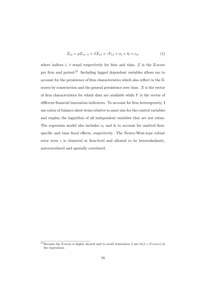
Zi,t = ρZi,t−1 + βXi,t + γYi,t + αi + δt + εi,t (1)
where indices i, t stand respectively for firm and time, Z is the Z-score
per firm and period.21 Including lagged dependent variables allows me to
account for the persistence of firm characteristics which also reflect in the Z-
scores by construction and the general persistence over time. X is the vector
of firm characteristics for which data are available while Y is the vector of
different financial innovation indicators. To account for firm heterogeneity, I
use ratios of balance sheet items relative to asset size for the control variables
and employ the logarithm of all independent variables that are not ratios.
The regression model also includes αi and δt to account for omitted firm-
specific and time fixed effects, respectively. The Newey-West-type robust
error term ε is clustered at firm-level and allowed to be heteroskedastic,
autocorrelated and spatially correlated.
21Because the Z-score is highly skewed and to avoid truncation, I use ln(1 + Z-score) inthe regressions.
18

5 Results
In this section, I discuss the main results and perform a number of robustness
checks. I also extend the model to further investigate the innovation-fragility
view in more detail.
5.1 Baseline Model
I compare different versions of the dynamic panel model set up in Section
4.2 which enhances the static linear fixed effects model by including autore-
gressive coefficients for fragility. This allows me to capture feedback from
current or past shocks to current values of the dependent variable. This
specification is adequate in the presence of autocorrelated error terms and
high persistence in the dependent variable which I have shown earlier.
Table 2 provides the overview of the different model specifications. Baseline
innovative capacity in firms is captured by firm size, profitability and lever-
age which Lerner (2006) has shown to be important drivers of incentives to
innovate. In all regressions, I include firm characteristics, year fixed effects
and a constant but suppress their coefficients in the tables.
Column 1 to 4 provides the Driscoll-Kraay (1998) estimator with firm fixed
effects and lagged dependent variables interchangeably. Column 4 depicts
the full model specification presented in Section 4.2. Even though firm fixed
effects cover average innovative ability of a firm while lagged dependent vari-
ables capture time trends, the γ coefficients to measure FI remain negative
and statistically significant. Once accounting for firm differences and time
trends, patenting becomes sufficiently less important for firm stability.
19

Tab
le2:
Var
iants
inth
eM
odel
Sp
ecifi
cati
on
stati
cfi
rmF
Eon
lyL
DV
on
lyfu
llsp
ecifi
cati
on
pre
-1998
com
peti
tion
ln(1
+Z
-score
t)ln
(1+
Z-s
core
t)ln
(1+
Z-s
core
t)ln
(1+
Z-s
core
t)ln
(1+
Z-s
core
t)ln
(1+
Z-s
core
t)
ln(1
+Z
-sco
ret−
1)
0.79
4***
0.01
3-0
.005
0.01
2(0
.060
)(0
.008
)(0
.008
)(0
.007
)ln
(ass
ets)
0.38
2***
-0.1
33**
*0.
111*
**-0
.139
***
-0.1
66**
*-0
.138
***
(0.0
27)
(0.0
11)
(0.0
32)
(0.0
09)
(0.0
08)
(0.0
09)
EB
ITD
A/r
even
ues
0.01
6***
-0.0
000.
005*
**-0
.000
0.00
0-0
.000
(0.0
02)
(0.0
00)
(0.0
01)
(0.0
00)
(0.0
00)
(0.0
00)
Lev
erag
era
tio
0.14
4-0
.266
***
-0.0
85*
-0.2
57**
*-0
.246
***
-0.2
54**
*(0
.162
)(0
.026
)(0
.051
)(0
.020
)(0
.025
)(0
.020
)H
HI
0.162
(0.4
35)
FI
by
oth
ers
-0.0
100.
003*
**-0
.003
*0.
001*
0.00
00.
001*
(0.0
08)
(0.0
01)
(0.0
02)
(0.0
01)
(0.0
01)
(0.0
01)
Inn
ovat
ion
s-0
.211
***
-0.0
28**
-0.0
75*
-0.0
29**
-0.0
58*
-0.0
27**
(0.0
34)
(0.0
12)
(0.0
42)
(0.0
12)
(0.0
31)
(0.0
12)
Pat
ents
-0.0
74**
*-0
.006
-0.0
16*
-0.0
040.
015
-0.0
04(0
.012
)(0
.006
)(0
.009
)(0
.005
)(0
.009
)(0
.005
)A
pp
lica
tion
s-0
.023
**-0
.003
0.00
2-0
.001
-0.0
03-0
.002
(0.0
12)
(0.0
05)
(0.0
06)
(0.0
05)
(0.0
05)
(0.0
05)
Con
trol
sY
YY
YY
YY
ear
FE
YY
YY
YY
Fir
mF
EN
YN
YY
YC
onst
ant
YY
YY
YY
Ob
serv
atio
ns
16,7
1716
,717
14,7
7014
,770
7,93
414
,770
Nu
mb
erof
firm
s2,
715
2,71
52,
660
2,66
02,
022
2,660
R-s
qu
ared
0.29
30.
594
0.55
10.
633
0.62
90.
633
Not
es:
See
Tab
leA
1in
the
Ap
pen
dix
for
defi
nit
ion
sof
the
vari
able
s.C
ount
dat
aon
inn
ovat
ion
sco
mes
from
the
Wal
lS
tree
tJou
rnal,
the
Fac
tiva
dat
abas
eor
the
US
Pat
ent
and
Tra
dem
ark
Offi
ce,
coll
ecte
dby
Ler
ner
(200
6).
All
fin
anci
ald
ata
isin
mil
lion
2002
US
Dol
lars
and
com
esfr
omC
omp
ust
at.
Col
um
n1
does
not
incl
ud
ea
lagg
edd
epen
den
tva
riab
leor
firm
fixed
effec
ts.
Col
um
n2
incl
ud
eson
lyfi
rmfi
xed
effec
ts.
Col
um
n3
incl
ud
eson
lya
lagg
edd
epen
den
tva
riab
le.
Col
um
n4
incl
ud
esth
efu
llm
od
elsp
ecifi
cati
onp
rese
nte
din
Sec
tion
4.2.
Col
um
n5
incl
ud
esd
ata
for
1990
unti
l19
98on
ly.
Col
um
n6
incl
ud
esd
ata
for
the
full
per
iod
from
1990
unti
l20
02w
ith
the
HH
Ico
ntr
olli
ng
for
firm
-lev
elco
mp
etit
ion
.In
all
regr
essi
ons,
Iin
clud
efi
rmch
arac
teri
stic
sas
contr
ols,
year
fixed
effec
tsan
da
con
stan
tb
ut
sup
pre
ssth
eir
coeffi
cien
tsin
the
table
s.C
ontr
olva
riab
les
incl
ud
efi
rmag
e,ca
sheq
uiv
alen
ts,
emp
loyee
s,re
tain
edea
rnin
gs,
shar
ehol
der
s’eq
uit
y,p
refe
rred
stock
and
lon
g-te
rmd
ebt
(all
asra
tios
rela
tive
toas
sets
orlo
gari
thm
s).
Dri
scol
l-K
raay
(199
8)ro
bu
stst
and
ard
erro
rsar
ecl
ust
ered
atfi
rm-l
evel
and
pre
sente
din
par
enth
eses
.**
*p<
0.01
,**
p<
0.05
,*
p<
0.1.
20

Column 5 presents the results for the period 1990 until 1998 only. Remem-
ber the State Street decision by the CAFC in 1998.22 This has provided
firms with legal certainty about what kind of FI can be legally protected.
Hence, more technology spillovers should theoretically be observed in the
pre-1998 period because of the legal uncertainty prior to the CAFC deci-
sion. Given these spillovers from FI, I expect to observe a stronger relation
between firm instability and innovative activity. I split the data sample into
pre-State Street and post-State Street periods. Analyzing the subsample in-
deed shows larger γ coefficients of the FI measures prior to 1998 and hence
confirms that the spillover effect of FI further decreases stability.
Moreover, I analyze the impact of competitive pressure on the proposed
positive relationship between FI and fragility. I thus include the Herfindahl-
Hirschman Index (HHI) in column 6. Because an increase in the HHI signals
rising market power and weakening competition, the positive regression co-
efficient for the HHI indicates that competition and stability are negatively
correlated which is the same conjecture Allen and Gale (2004) made. Con-
trolling for competition does not change the γ coefficients of the FI measures
or the agglomeration effect.
Overall, results show that indeed there exists a significant positive relation
between FI and fragility (negative relation between FI and Z-scores) albeit
small, but patenting seems to be no factor. The size of the coefficients how-
ever corresponds to the correlations from the univariate analyses in Section
4.1. Surprisingly, the agglomeration effect as measured in FI by others is
very weak.
22I already mentioned this in the Literature Review (Section 2) and it is discussed inLerner (2002).
21

5.2 Robustness
I check the robustness of my results. Foremost, the results in Table 2 are ro-
bust against including or excluding different firm-specific control variables.
I also use data on revenues and common market value instead of total assets
to control for firm size but the results do not change. If I include a dummy
variable for incidences of FI instead of the three different count measures,
the coefficient is negative but not significant.
In order to check whether my results are due to a particular econometric
specification, I run different panel estimators. I compare my baseline model
specification to a pooled feasible GLS estimator with a panel-specific AR(1)-
disturbance, a Prais-Winsten regression to account for autocorrelated error
terms, and a Newey-West heteroskedasticity- and autocorrelation-consistent
(HAC) estimator. I find qualitatively similar results. The advantage of
Driscoll-Kraay (1998) standard errors is that they expand Newey-West HAC
estimators to include correlation between panels and that the estimator does
not place restrictions on the limit behavior of the number of panels.
I also run dynamic panel data estimators. I use the Arellano-Bond (1991)
estimator by instrumental-variables (IV) estimation of the parameters of the
first-difference model using lags of regressors as instruments.23 Additionally,
I use the Blundell-Bond (1998) estimator because the Arellano-Bond (1991)
estimator performs poorly with large autoregressive disturbances.24 I find
23I have shown earlier that the data is trend stationary. Because the Arellano-Bond (1991)estimator relies on first differences, it consumes most of the variation between observa-tions for innovation indicators since their within-variation (variation over time) is largerthan their variation between panels. Thus, coefficients for the innovation indicators turnout smaller and not significant in the regression.
24The Blundell-Bond (1998) estimator is a system GMM estimation method which en-hances the Arellano-Bond (1991) estimator with additional moment conditions. Both
22

qualitatively similar results.
In any estimation of fixed effects models for short panels when lagged de-
pendent variables are present, coefficients may be downwardly biased. This
is called Nickell (1981) Bias whose size is relative to the time period T of the
data set. It is given here by 1/T = 1/13 = 0.07. Thus, as T → ∞ the bias
disappears.25 That’s why I compare the Driscoll-Kraay (1998) estimator
with the aforementioned dynamic panel data estimators which are consis-
tent. Two caveats arise from dynamic panel data estimators in this case,
namely that the IV estimation greatly increases the mean squared error and
that errors are assumed to not be serially correlated. On the other hand, the
Driscoll-Kraay (1998) estimator works with great precision although poten-
tially biased. Thus, a trade-off between correcting biases against decreases
in efficiency is inherent. Fundamentally, trading a small reduction in the
bias for a large decrease in efficiency sounds questionable. Assuming the
Nickell (1981) bias is negligible since T = 13 is a reasonable time period and
given the small coefficient for lagged Z-scores from Table 2, I further pursue
the Driscoll-Kraay (1998) estimator with fixed effects and lagged dependent
variables in my analysis.
5.3 Extensions
I extend the baseline model with a couple features. First, I want to explore
the relationship between innovation and fragility across firms with differ-
ent characteristics. Thus, I generate interaction terms of the FI measures
estimators are consistent, but they assume that there exists no autocorrelation in theerror terms, that panel-level effects are uncorrelated with the first differences and thatgood instruments are available.
25Compare Behr (2003) for a discussion of dynamic panel data estimators and their ap-plication to financial data.
23

with assets, profitability and leverage.26 Table 3 provides the piece-wise
inclusion of these interactions into the regression with the Driscoll-Kraay
(1998) estimator assessed above. Column 1 and 4 show the effect of FI on
fragility with heterogeneous firm size. The relationship is stronger for larger
banks but only for innovative activity captured through patenting. Overall,
patenting decreases stability significantly. Column 2 and 4 show that the
different profitability levels have no impact on the effect of FI on fragility as
expected. Finally, column 3 and 4 display the effect of FI on fragility with
different leverage ratios. The relationship is stronger when firms are more
leveraged and the impact of innovation increases with the leverage ratio.
Across all models, the positive (negative) relation between innovation and
fragility (stability) prevails, while the size of the coefficients differs across
specifications.
Second, I investigate the robustness of my results from Section 3.4 against
modifications of innovation measures as depicted in Table 4. Column 1 pro-
vides the regression results with the Driscoll-Kraay (1998) estimator from
Table 2. Subsequently, column 2 uses a weighting mechanism to account
for sole or collaborative inventions, column 3 uses only highly innovative
activities as classified by a three-part scheme introduced by Lerner (2006),
column 4 provides a combination of 2 and 3 and finally, column 5 introduces
R&D expenditures as a further control.27 Results are confirmed. The pos-
itive relation between innovation and fragility is persistent while patenting
has no effect.
26For the interaction terms, I multiply my FI indicators with assets, profitability andleverage, respectively.
27See Table A1 in the Appendix for a description of the exact modifications.
24

Table 3: Interaction with Firm Characteristics
Firm Size Profitability Leverage CompoundModel
ln(1+Z-scoret) ln(1+Z-scoret) ln(1+Z-scoret) ln(1+Z-scoret)
ln(1+Z-scoret−1) 0.013* 0.013* 0.013* 0.013*(0.008) (0.008) (0.008) (0.008)
ln(assets) -0.155*** -0.155*** -0.154*** -0.154***(0.013) (0.013) (0.013) (0.013)
EBITDA/revenues 0.000 0.000 0.000 0.000(0.000) (0.000) (0.000) (0.000)
Leverage ratio -0.228*** -0.227*** -0.227*** -0.227***(0.024) (0.024) (0.025) (0.025)
FI by others in 2-digit zip code 0.002* 0.002* 0.002* 0.002(0.001) (0.001) (0.001) (0.001)
Innovations -0.016 -0.010*** -0.103** -0.097***(0.019) (0.004) (0.043) (0.034)
Patents -0.042*** 0.002 -0.036* -0.035**(0.012) (0.005) (0.020) (0.017)
Applications -0.016 -0.008* -0.044 -0.060*(0.012) (0.005) (0.033) (0.035)
Innovations * ln(assets) -0.048 0.191(0.158) (0.195)
Patents * ln(assets) -0.402*** -0.672***(0.111) (0.195)
Applications * ln(assets) -0.136 -0.029(0.091) (0.081)
Innovations * EBITDA/revenues 0.001 0.001(0.001) (0.001)
Patents * EBITDA/revenues -0.001*** -0.002***(0.000) (0.000)
Applications * EBITDA/revenues -0.001 -0.001*(0.000) (0.000)
Innovations * leverage ratio -0.117** -0.139**(0.052) (0.054)
Patents * leverage ratio -0.035 0.027(0.022) (0.020)
Applications * leverage ratio -0.046 -0.055(0.033) (0.041)
Controls Y Y Y YYear FE Y Y Y YFirm FE Y Y Y YConstant Y Y Y Y
Observations 14,770 14,770 14,770 14,770Number of firms 2,660 2,660 2,660 2,660R-squared 0.634 0.634 0.634 0.634
Notes: See Table A1 in the Appendix for definitions of the variables. Count data on innovations comes fromthe Wall Street Journal, the Factiva database or the US Patent and Trademark Office, collected by Lerner(2006). All financial data is in million 2002 US Dollars and comes from Compustat. All columns incorporatethe baseline model from column 4 of Table 2. Column 1 includes interaction terms between firm size and FImeasures. Column 2 includes interaction terms between profitability and FI measures. Column 3 includesinteraction terms between leverage ratio and FI measures. Finally, column 4 includes all interaction terms. Inall regressions, I include firm characteristics as controls, firm and year fixed effects, and a constant but suppresstheir coefficients in the tables. Control variables include firm age, cash equivalents, employees, retained earnings,shareholders’ equity, preferred stock and long-term debt (all as ratios relative to assets or logarithms). Driscoll-Kraay (1998) robust standard errors are clustered at firm-level and presented in parentheses. *** p<0.01, **p<0.05, * p<0.1.
25

Tab
le4:
Rob
ust
nes
sag
ain
stF
IM
easu
res
base
weig
hte
dm
ajo
rw
eig
hte
dR
&D
an
dm
ajo
rln
(1+
Z-s
core
t)ln
(1+
Z-s
core
t)ln
(1+
Z-s
core
t)ln
(1+
Z-s
core
t)ln
(1+
Z-s
core
t)
ln(1
+Z
-sco
ret−
1)
0.01
30.
013
0.01
30.0
13
0.0
13
(0.0
08)
(0.0
08)
(0.0
08)
(0.0
08)
(0.0
08)
ln(a
sset
s)-0
.139
***
-0.1
39**
*-0
.139
***
-0.1
39**
*-0
.143**
*(0
.009
)(0
.009
)(0
.009
)(0
.009)
(0.0
08)
EB
ITD
A/r
even
ues
-0.0
00-0
.000
-0.0
00-0
.000
0.0
00
(0.0
00)
(0.0
00)
(0.0
00)
(0.0
00)
(0.0
00)
Lev
erag
era
tio
-0.2
57**
*-0
.257
***
-0.2
58**
*-0
.258
***
-0.2
48**
*(0
.020
)(0
.020
)(0
.020
)(0
.020)
(0.0
18)
FI
by
other
sin
2-dig
itzi
pco
de
0.00
1*0.
001*
0.00
1*0.0
01*
0.001
*(0
.000
)(0
.000
)(0
.000
)(0
.000)
(0.0
00)
Innov
atio
npar
amet
ers
-0.0
29**
-0.0
46**
*-0
.028
*-0
.051*
-0.0
27**
(0.0
12)
(0.0
17)
(0.0
15)
(0.0
27)
(0.0
12)
Pat
ent
par
amet
ers
-0.0
04-0
.012
-0.0
05-0
.014
-0.0
06
(0.0
05)
(0.0
14)
(0.0
05)
(0.0
14)
(0.0
05)
Applica
tion
par
amet
ers
-0.0
01-0
.004
-0.0
01-0
.004
-0.0
01
(0.0
05)
(0.0
15)
(0.0
05)
(0.0
15)
(0.0
05)
R&
D/a
sset
s-0
.489***
(0.1
44)
Con
trol
sY
YY
YY
Yea
rF
EY
YY
YY
Fir
mF
EY
YY
YY
Con
stan
tY
YY
YY
Obse
rvat
ions
14,7
7014
,770
14,7
7014,
770
14,7
70
Num
ber
offirm
s2,
660
2,66
02,
660
2,6
60
2,6
60
R-s
quar
ed0.
633
0.63
30.
633
0.633
0.6
34
Not
es:
See
Tab
leA
1in
the
App
endix
for
defi
nit
ions
ofth
eva
riab
les.
Cou
nt
dat
aon
innov
atio
ns
com
esfr
om
the
Wal
lStr
eet
Jou
rnal
,th
eF
acti
vadat
abas
eor
the
US
Pat
ent
and
Tra
dem
ark
Offi
ce,
collec
ted
by
Ler
ner
(2006
).A
llfinanci
al
data
isin
million
2002
US
Dol
lars
and
com
esfr
omC
ompust
at.
Col
um
n1
inco
rpor
ates
the
bas
elin
em
odel
from
colu
mn
4of
Table
2.C
olu
mn
2in
cludes
aw
eigh
ting
mec
han
ism
toac
count
for
sole
orco
llab
orat
ive
inve
nti
ons.
Col
um
n3
incl
udes
only
hig
hly
innov
ati
veac
tivit
ies
ascl
assi
fied
by
ath
ree-
par
tsc
hem
ein
troduce
dby
Ler
ner
(200
6).
Col
um
n4
isa
com
bin
ati
on
of
2and
3.It
incl
udes
aw
eigh
ting
mec
han
ism
toac
count
for
sole
orco
llab
orat
ive
inven
tion
sof
only
hig
hly
innov
ati
veact
ivit
ies
as
class
ified
by
Ler
ner
(200
6).
Fin
ally
,co
lum
n5
incl
udes
R&
Dex
pen
dit
ure
sas
afu
rther
contr
ol.
Inal
lre
gres
sions,
Iin
clude
firm
char
act
eris
tics
asco
ntr
ols,
firm
and
year
fixed
effec
ts,
and
aco
nst
ant
but
suppre
ssth
eir
coeffi
cien
tsin
the
table
s.C
ontr
ol
vari
able
sin
clude
firm
age,
cash
equiv
alen
ts,
emplo
yees
,re
tain
edea
rnin
gs,
shar
ehol
der
s’eq
uit
y,pre
ferr
edst
ock
and
long-t
erm
deb
t(a
llas
rati
osre
lati
veto
asse
tsor
loga
rith
ms)
.D
risc
oll-
Kra
ay(1
998)
robust
stan
dar
der
rors
are
clust
ered
atfirm
-lev
eland
pre
sente
din
pare
nth
eses
.**
*p<
0.01
,**
p<
0.05
,*
p<
0.1.
26

Third, I further explore the robustness of results by investigating the compo-
nents of the Z-score and alternative measures for firm fragility in Table 5.28
Thus, I keep the right-hand side variables the same and compare different
left-hand side variables. I respectively use ROA, ROE and the capital-asset
ratio to assess profitability and capitalization, the volatility of ROA and
volatility of ROE to measure a firm’s activity risk, and finally, the Sharpe
ratio as an alternative measure for the risk of insolvency. Specifically, the
Sharpe ratio describes how well the return compensates the investor for the
risk taken. Column 2 and 3 show that profitability is positively affected
by patenting behavior, but surprisingly, the innovation coefficient is signifi-
cantly negative although small. Capitalization in column 4 negatively affects
firm stability on a small scale, but only in patenting. Unusually, activity
risk is not affected by a firm’s degree of innovation as depicted in columns 5
and 6. Lastly, innovation continues to positively relate to risk of insolvency
although the coefficient becomes insignificant whereas unexpectedly patent-
ing positively affects excessive returns as shown in column 7.
Fourth, another investigation looks at the impact of FI on profitability dur-
ing a financial crisis. Did FI hurt financial institutions during a period of
financial market breakdown? In a cross-sectional setting where independent
variables from 1999 only are used, I analyze whether firms make larger losses
during financial distress when innovating. Table 6 provides an overview of
the summary statistics of the variables for 1999. The cross-sectional sample
has 1,781 observations. For most variables, mean values are larger than the
median indicating a few large firms drive up average values. Values for most
differences in profitability are negative. Variances in general are large.
28Because the different measures are highly skewed and to avoid truncation, I use thelogarithm for the dependent variables in the regressions, except for standard deviations.
27

Tab
le5:
Rob
ust
nes
sag
ain
stF
ragi
lity
Mea
sure
s
(1)
(2)
(3)
(4)
(5)
(6)
(7)
ln(1
+Z
-score
t)ln
(1+
RO
At)
ln(1
+R
OE
t)ln
(1+
CA
Rt)
σ(R
OA
)σ(R
OE
)ln
(1+
Sh
arp
et)
ln(1
+Z
-sco
ret−
1)
0.0
13(0
.008
)ln
(1+
RO
At−
1)
0.042
(0.0
22)
ln(1
+R
OEt−
1)
0.02
4(0
.015
)ln
(1+
CA
Rt−
1)
0.32
7**
*(0
.004)
ln(1
+Shar
pe t−1)
0.0
33**
*(0
.009)
ln(a
sset
s)-0
.143*
**
0.00
4-0
.152
***
-0.0
48***
-0.0
20-0
.083
-0.2
97***
(0.0
08)
(0.0
07)
(0.0
22)
(0.0
05)
(0.0
17)
(0.0
66)
(0.0
24)
EB
ITD
A/r
even
ues
0.000
0.0
00**
*0.
001
***
0.000
0.0
00-0
.000
-0.0
01(0
.000
)(0
.000
)(0
.000)
(0.0
00)
(0.0
00)
(0.0
00)
(0.0
01)
Lev
erag
era
tio
-0.2
48***
0.00
50.
091**
*0.
100
***
-0.0
11-0
.158
0.1
66***
(0.0
18)
(0.0
13)
(0.0
15)
(0.0
06)
(0.0
14)
(0.1
32)
(0.0
55)
FI
by
other
sin
2-dig
itzi
pco
de
0.00
1*0.0
010.0
030.0
010.
009
0.0
02
0.0
00
(0.0
00)
(0.0
01)
(0.0
02)
(0.0
01)
(0.0
07)
(0.0
01)
(0.0
03)
Innov
atio
ns
-0.0
27*
*-0
.003
**
-0.0
04-0
.002
-0.0
01-0
.037
-0.0
26
(0.0
12)
(0.0
01)
(0.0
06)
(0.0
03)
(0.0
04)
(0.0
42)
(0.0
27)
Pat
ents
-0.0
060.
003
0.00
9**
-0.0
03***
-0.0
020.0
01
0.0
18**
(0.0
05)
(0.0
02)
(0.0
04)
(0.0
01)
(0.0
02)
(0.0
03)
(0.0
09)
Applica
tion
s-0
.001
0.00
3**
0.0
07**
-0.0
02*
*-0
.002
0.0
02
0.0
18***
(0.0
05)
(0.0
01)
(0.0
03)
(0.0
01)
(0.0
02)
(0.0
02)
(0.0
06)
R&
D/a
sset
s-0
.489*
**
-0.4
49-0
.498
***
0.0
730.
159
0.0
02
-0.2
53**
(0.1
44)
(0.5
04)
(0.1
36)
(0.0
55)
(0.1
52)
(0.0
85)
(0.1
24)
Con
trol
sY
YY
YY
YY
Yea
rF
EY
YY
YY
YY
Fir
mF
EY
YY
YY
YY
Con
stan
tY
YY
YY
YY
Obse
rvat
ions
14,
770
14,7
7014
,754
14,8
2414
,770
14,5
05
13,9
60
Num
ber
offirm
s2,
660
2,66
02,
658
2,71
42,
660
2,6
59
2,6
30
R-s
quar
ed0.6
340.1
030.
071
0.51
90.
004
0.0
02
0.082
Not
es:
See
Tab
leA
1in
the
App
endix
for
defi
nit
ions
ofth
eva
riab
les.
Cou
nt
data
onin
nov
ati
ons
com
esfr
om
the
Wal
lStr
eet
Journ
al,
the
Fac
tiva
dat
abas
eor
the
US
Pate
nt
and
Tra
dem
ark
Offi
ce,
collec
ted
by
Ler
ner
(200
6).
All
finan
cial
dat
ais
inm
illion
2002
US
Dollars
and
com
esfr
omC
ompust
at.
Lag
ged
dep
enden
tva
riab
les
are
incl
uded
inth
ere
gre
ssio
ns
exce
pt
for
stan
dar
ddev
iati
ons
of
retu
rns.
Ike
epall
oth
erin
dep
enden
tva
riab
les
the
sam
ean
don
lych
ange
the
dep
enden
tva
riab
les
from
colu
mn
toco
lum
n.
Colu
mn
1in
corp
ora
tes
the
bas
elin
em
odel
from
colu
mn
4of
Tab
le2.
Col
um
n2
and
3m
easu
reth
eim
pac
tof
FI
on
pro
fita
bilit
yw
her
ere
turn
son
asse
tsan
deq
uit
yare
the
dep
enden
tva
riab
les,
resp
ecti
vely
.C
olum
n4
mea
sure
sth
eim
pac
tof
FI
onca
pit
aliz
atio
nof
form
s.H
ere,
the
capit
al-a
sset
rati
ois
the
dep
enden
tva
riable
.C
olum
n5
and
6m
easu
reth
eim
pac
tof
FI
onac
tivit
yri
skby
incl
udin
gth
est
andard
dev
iati
ons
ofth
ere
turn
son
asse
tsand
equit
y,re
spec
tive
ly.
For
thes
etw
ore
gres
sions
coeffi
cien
tsar
esc
aled
by
1,0
00.
Fin
ally,
colu
mn
7in
cludes
the
Shar
pe
Rat
ioas
dep
enden
tva
riable
as
anoth
erst
abilit
ym
easu
re.
Inal
lre
gres
sions,
Iin
clude
firm
char
acte
rist
ics
as
contr
ols,
firm
and
year
fixed
effec
ts,
and
aco
nst
ant
but
suppre
ssth
eir
coeffi
cien
tsin
the
table
s.C
ontr
ol
vari
able
sin
clude
firm
age,
cash
equiv
alen
ts,
emplo
yees
,re
tain
edea
rnin
gs,
shar
ehol
der
s’eq
uit
y,pre
ferr
edst
ock
and
long-t
erm
deb
t(a
llas
rati
osre
lati
veto
asse
tsor
logar
ithm
s).
Dri
scol
l-K
raay
(1998
)ro
bust
standard
erro
rsar
ecl
ust
ered
atfirm
-lev
elan
dpre
sente
din
par
enth
eses
.**
*p<
0.01,
**p<
0.0
5,*
p<
0.1.
28

Table 6: Summary Statistics of Cross-Section (1999)
Variable Mean Median Std. Dev. Min. Max.
Age 9.226 5.000 11.699 0 74Assets 15381.500 614.032 65763.220 0 893649Cash Equiv. 1503.317 27.252 9642.401 0 205371Leverage 0.326 0.293 0.276 0 0.997Long-term Debt 1954.220 51.799 12102.890 0 339221Market Value 4597.746 116.612 26350.170 0.062 535947Pref. Stock 33.535 0.000 183.772 0 3375Revenues 2802.985 79.385 12301.180 0 184589Sh. Equity 1496.865 87.944 5640.443 -44 83397
∆(Opprof) -0.533 0.014 16.200 -523.908 130.719∆(ROA) -0.096 -0.001 1.382 -41.827 1.671∆(ROE) 0.195 -0.004 6.999 -51.006 230.774
Innovations (avg.) 0.012 0.000 0.075 0 1.200Patents (avg.) 0.024 0.000 0.219 0 5.000Applications (avg.) 0.040 0.000 0.352 0 7.000R&D 48.874 0.000 457.900 0 7502.168FI by others 1.002 0.000 1.713 0 4.000
Notes: N=1,781. See Table A1 in the Appendix for definitions of the variables.All financial data is in million 2002 US Dollars and comes from Compustat.Count data on innovations comes from the Wall Street Journal, the Factivadatabase or the US Patent and Trademark Office, collected by Lerner (2006).FI measures are averaged over the period 1990 to 1999.
For the cross-sectional analysis, I use as the dependent variable ∆(Opprof),
∆(ROA) and ∆(ROE), respectively, where ∆(�) = (�)2002 − (�)1999.29 I
expect that the difference will be negative for most firms and should be larger
for more innovative firms. The model specification for the three regressions
is as follows.
∆(�)i = βXi + γYi + εi (2)
where index i stands for the firm and the dependent variable is the perfor-
mance change between 2002 and 1999 calculated as the difference in ROA,
ROE, Opprof = EBITDA/revenues, respectively, between the values in
29The year 1999 has the most observations per year in the data set and the NASDAQ hadits ten-year peak then, while in 2002 the NASDAQ considerably dropped because of theburst of the ICT bubble.
29

the respective years. Again, X is the vector of firm characteristics in 1999
while Y is the vector of different financial innovation indicators. I use fea-
sible GLS estimation with heteroskedastic error terms ε in the regressions.
FI measures are averaged over the period 1990 to 1999 because this cap-
tures overall innovative activity per firm. Table 7 provides the results which
suggest that more innovative firms face higher profitability declines dur-
ing distress. The significantly negative sign on γ is consistent with the
innovation-fragility view and suggests that firms with higher FI suffered
more in a crisis.
30

Table 7: Comparison of Profitability Changes
(1) (2) (3)∆(ROA) ∆(ROE) ∆(Opprof)
Log of assets 0.044*** -0.329*** -0.279***(0.002) (0.008) (0.019)
EBITDA/revenues 0.010*** -0.008(0.003) (0.011)
Leverage ratio -0.152*** 1.190*** 0.675***(0.004) (0.029) (0.047)
FI by others in 2-digit zip code -0.040*** 0.041*** -0.150***(0.005) (0.002) (0.016)
Innovations (avg.) -0.087*** -0.315*** -1.634***(0.006) (0.021) (0.178)
Patents (avg.) -0.511*** 0.366*** -1.696***(0.028) (0.060) (0.543)
Applications (avg.) 0.249*** -0.223*** 0.751**(0.018) (0.037) (0.302)
Controls Y Y YConstant Y Y Y
Observations 1,202 1,201 1,196Number of firms 1,202 1,201 1,196R-squared 0.044 0.048 0.023
Notes: See Table A1 in the Appendix for definitions of the variables.Count data on innovations comes from the Wall Street Journal, theFactiva database or the US Patent and Trademark Office, collected byLerner (2006). FI measures are averaged over the period 1990 to 1999.All financial data is in million 2002 US Dollars and comes from Com-pustat. In column 1, I use the change in ROA as dependent variable, incolumn 2, I use the change in ROE as dependent variable, and finally,in column 3, I use the change in operational profitability as dependentvariable. In all regressions, I include firm characteristics as controls anda constant but suppress their coefficients in the tables. Control vari-ables include firm age, cash equivalents, employees, retained earnings,shareholders’ equity, preferred stock and long-term debt (all as ratiosrelative to assets or logarithms). Robust standard errors are clusteredat firm-level and presented in parentheses. *** p<0.01, ** p<0.05, *p<0.1.
31

6 Conclusion
In this paper, I evaluate the relationship between financial innovations and
the fragility of financial institutions. Theoretical literature provides strong
evidence for why financial crises exist and why firms engage in producing
financial innovations. A recent strand of research tries to combine both ar-
eas and analyzes the impact of innovative activity of financial agents in a
competitive framework. Particularly, this mostly theoretical literature links
profit volatility to innovative activities and predicts a positive relationship.
That is, the degree of innovation negatively affects firm stability.
I base my analysis on a unique data set that counts financial innovations in
the USA between 1990 and 2002 provided by Lerner (2006) and augment it
by performance and stability measures. Then, I build on empirical frame-
works by Beck et al. (2012) and others to quantitatively assess the so called
innovation-fragility view on a firm level. I can show that a larger degree of
innovation positively (negatively) affects firm fragility (stability) after con-
trolling for the underlying firm characteristics. A couple of extensions to the
initial model show that my results are quite robust. Different modifications
of the innovation measures yield the same outcomes. Furthermore, I use
different fragility parameters measuring profitability, capitalization, activity
risk and risk of insolvency and find that the results support my argumen-
tation. In addition, firms with higher pre-crisis FI face higher losses during
a period of financial crisis. Overall, my analyses support the innovation-
fragility view.
Further research could include applying VAR models that take greater ac-
count for the persistence in firm characteristics and causality. Expanding
32

the time dimension may make the analysis more robust while cross-country
comparisons could provide policy recommendations. Additionally, insights
into the dynamics of innovative activity could be deduced from a structural
approach to modelling FI.
33

Appendix
Table A1: Overview of Variables, Definitions and Sources
Variables Definitions Sources30
Financial innovation measuresApplications Patent applications counted per
firm in a year.US PTO31, col-lected by Lerner(2006)
Applications-wt Weighted patent applicationsper firm in a year where the sumof 1 (count) is divided amongthe firms mentioned in the ar-ticle about the innovation.
US PTO, col-lected by Lerner(2006)
Innovations Count of stories from newspa-per articles and databases on in-novations per firm in a year.
WSJ32 and FD33,collected byLerner (2006)
Innovations-wt Weighted count of innovations(as above).
WSJ and FD, col-lected by Lerner(2006)
Innovations-ab Count of only major innova-tions where Lerner (2006) ap-plies a three-part classificationscheme (A,B,C).
WSJ and FD, col-lected by Lerner(2006)
Innovations-wt-ab Weighted count of major inno-vations (as above).
WSJ and FD, col-lected by Lerner(2006)
FI by Others Number of financial innovationsin the same year by other firmswith headquarters in the sametwo-digit zip code as the firm.
WSJ and FD, col-lected by Lerner(2006)
Patents Count of patents granted to afirm in a year with respect tothe financial services area.
US PTO, col-lected by Lerner(2006)
Patents-wt Weighted count of patents (asabove).
US PTO, col-lected by Lerner(2006)
30I make use of the data set constructed by Lerner (2006) for which he draws on variousdata sources. In addition, I define and compute additional factors, which were previouslynot used, for my empirical investigation. All financial data is in million 2002 US Dollars.
31US Patent and Trademark Office32Wall Street Journal33Factiva database
34

Financial Institution’s performance measuresEBIT Earnings before interest and
taxes per firm and year.Compustat
EBITDA Earnings before interest, taxes,depreciation and amortizationper firm and year.
Compustat
Net Income Net income of a firm in million2002 USD per year.
Compustat
Opprof Operational profitability con-structed as EBITDA / revenues(opprof = EBIT / revenues,whenever EBITDA is unavail-able).
computed fromCompustat data
Ret. Earnings Retained earnings in million2002 USD per firm in a year.
Compustat
ROA Return on assets constructed asnet income / assets.
computed fromCompustat data
ROE Return on equity constructed asnet income / shareholders’ eq-uity.
computed fromCompustat data
Financial Institution’s stability measuresCAR Capital-asset ratio constructed
as shareholders’ equity / assets.computed fromCompustat data
∆(Opprof) Difference between operationalprofitability in 2002 and 1999.
computed fromCompustat data
∆(ROA) Difference between return onassets in 2002 and 1999.
computed fromCompustat data
∆(ROE) Difference between return onequity in 2002 and 1999.
computed fromCompustat data
σ(ROA) Standard deviation of ROA foreach agent calculated over thesample period.
computed fromCompustat data
σ(ROE) Standard deviation of ROE foreach agent calculated over thesample period.
computed fromCompustat data
Sharpe Sharpe ratio constructed asROE / σ(ROE). Larger valuesimply less excessive risk for acertain return.
computed fromCompustat data
Z-score Index of bank solvency con-structed as (ROA+CAR) /σ(ROA). Higher Z-score implieslower probability of failure.
computed fromCompustat data
35

Other agent-level variablesAge Age of firm in relation to its
foundation or IPO.Compustat
Assets Total assets of each financial in-stitution in million 2002 USDper year.
Compustat
Cash equiv Cash equivalents in million 2002USD per firm in a year.
Compustat
Emp Employees per firm and year. CompustatHHI Herfindahl-Hirschman In-
dex defined as the sumof squared shares of rev-enues oer firm to total rev-enues per year, i.e. HHI =ΣNi (revenuesi/total revenues)2
per year.
computed fromCompustat data
Leverage Ratio of the book value of afirm’s long-term debt to to-tal capitalization (book valueof long-term debt and preferredstock and the market value ofcommon stock).
Compustat
Lt. Debt Long-term debt in million 2002USD per firm in a year.
Compustat
MV-common Common market value in mil-lion 2002 USD per firm in ayear.
Compustat
Pref. Stock Preferred stock in million 2002USD per firm in a year.
Compustat
R&D Expenditures per firm for re-search and development in mil-lion 2002 USD in a year.
Compustat
Revenues Revenues in million 2002 USDper firm in a year.
Compustat
Sh. Equity Shareholders’ equity in million2002 USD per firm in a year.
Compustat
36

Table
A2:
Sp
earm
an
Corr
ela
tion
Coeffi
cients
of
FI
measu
res
and
Z-s
core
sof
firm
s
Log
of
Inn
ovati
on
sW
eig
hte
dO
nly
Weig
hte
dP
ate
nts
Weig
hte
dA
pp
licati
on
sW
eig
hte
dR
&D
FI
by
z-s
core
cou
nts
of
majo
rm
ajo
rcou
nts
of
cou
nts
of
rati
ooth
ers
inn
ovati
on
sin
novati
on
sin
novati
on
sp
ate
nts
ap
plicati
on
s
Log
of—
z-sc
ore
Innov
atio
ns
-0.0
417*
**—
Wei
ghte
dco
unt
-0.0
417*
**1.
0000
***
—of
innov
atio
ns
Only
ma
jor
-0.0
338**
*0.
8397
***
0.83
90**
*—
innov
atio
ns
Wei
ghte
dm
ajo
r-0
.033
8***
0.83
97**
*0.
8390
***
1.00
00***
—in
nov
atio
ns
Pat
ents
-0.0
707*
**0.
1459
***
0.14
58**
*0.
1272
***
0.1
272*
**
Wei
ghte
dco
unt
-0.0
707*
**0.
1459
***
0.14
58**
*0.
1272
***
0.1
272*
**
1.0
000*
**—
ofpat
ents
Applica
tion
s-0
.056
1***
0.12
13**
*0.
1212
***
0.10
87***
0.1
088*
**0.
442
8**
*0.
442
8**
*—
Wei
ghte
dco
unt
-0.0
561*
**0.
1213
***
0.12
12**
*0.
1087
***
0.1
088*
**
0.4
428*
**0.
442
8**
*1.
0000
***
—of
applica
tion
s
R&
Dra
tio
-0.2
158*
**0.
1004
***
0.10
03**
*0.
0818
***
0.081
8***
0.34
31***
0.34
31**
*0.
2953
***
0.2
953***
—
FI
by
other
s-0
.018
7***
-0.0
336*
**-0
.033
7***
-0.0
270**
*-0
.027
1**
*-0
.016
8-0
.016
8-0
.0083
-0.0
083
-0.0
208***
—
Not
es:
***
p<
0.01
37

References
[1] Allen, F., A. Babus and E. Carletti (2009): ”Financial Crises: Theoryand Evidence”, Annual Review of Financial Economics, Vol. 1, pp. 97-116.
[2] Allen, F. and D. Gale (2000): ”Financial Contagion”, Journal of Polit-ical Economy, Vol. 108, No. 1, pp. 1-33.
[3] Allen, F. and D. Gale (2004): ”Competition and Financial Stability”,Journal of Money, Credit, and Banking, Vol. 36, No. 3, pp. 453-480.
[4] Allen, F. and A. Winton (1995): ”Corporate Financial Structure, In-centives and Optimal Contracting”, in: R. Jarrow, V. Maksimovic andW. Ziemba (eds.): Handbook of Operations Research and ManagementScience (Volume 9: Finance), Elsevier, Amsterdam, Netherlands, pp.693-720.
[5] Arellano, M. and S. Bond (1991): ”Some Tests of Specification forPanel Data: Monte Carlo Evidence and an Application to EmploymentEquations”, The Review of Economic Studies, Vol. 58, No. 2, pp. 277-297.
[6] Beck, T. H. L., T. Chen, C. Lin and F. M. Song (2012): ”FinancialInnovation: The Bright and the Dark Sides”, working paper, availableat SSRN: http://ssrn.com/abstract=1991216 .
[7] Behr, A. (2003): ”A Comparison of Dynamic Panel Data Estimators:Monte Carlo Evidence and an Application to the Investment Function”,Deutsche Bundesbank Discussion Paper 05/03.
[8] Bertay, A. C., A. Demirguc-Kunt and H. Huizinga (2013): ”Do we needbig banks? Evidence on performance, strategy and market discipline”,Journal of Financial Intermediation, forthcoming.
[9] Bhattacharyya, S. and V. Nanda (2000): ”Client Discretion, SwitchingCosts, and Financial Innovation”, The Review of Financial Studies, Vol.13, No. 4, pp. 1101-1127.
[10] Blundell, R. and S. Bond (1998): ”Initial Conditions and Moment Re-strictions in Dynamic Panel Data Models”, Journal of Econometrics,Vol. 87, pp. 115-143.
[11] Boz, E. and E. G. Mendoza (2010): ”Financial Innovation, the Discov-ery of Risk, and the US Credit Crisis”, NBER Working Paper 16020.
[12] Brunnermeier, M. K. (2009): ”Deciphering the Liquidity and CreditCrunch 2007-2008”, The Journal of Economic Perspectives, Vol. 23,No. 1, pp. 77-100.
38

[13] Carvajal, A., M. Rostek and M. Weretka (2012): ”Competition in Fi-nancial Innovation”, Econometrica, Vol. 80, No. 5, pp. 1895-1936.
[14] Demirguc-Kunt, A. and H. Huizinga (2010): Are Banks too Big to Failor too Big to Save? International Evidence from Equity Prices andCDS Spreads”, CEPR Discussion Paper 7903.
[15] Driscoll, J. C. and A. C. Kraay (1998) ”Consistent Covariance Ma-trix Estimation with Spatially Dependent Panel Data”, Review of Eco-nomics and Statistics, Vol. 80, pp. 549-560.
[16] Duffie D. and R. Rahie (1995): ”Financial Market Innovation and Se-curity Design: An Introduction”, Journal of Economic Theory, Vol 65,pp. 1-42.
[17] Ferreira, D., G. Manso and A. C. Silva (2012): ”Incentives to Innovateand the Decision to Go Public or Private”, Review of Financial Studies,forthcoming.
[18] Frank, W. S. and L. J. White (2004): ”Empirical Studies of Finan-cial Innovation: Lots of Talk, Little Action?”, Journal of EconomicLiterature, Vol. 42, No. 1, pp. 116-144.
[19] Frank, W. S. and L. J. White (2009): ”Technological Change, FinancialInnovation, and Diffusion in Banking”, working paper 2009-10, FederalReserve Bank of Atlanta.
[20] Gennaioli, N., A. Shleifer and R. W. Vishny (2012): ”Neglected Risks,Financial Innovation, and Financial Fragility”, Journal of FinancialEconomics, Vol. 104, pp. 452-468.
[21] Hasan, I., H. Schmiedel and L. Song (2009): ”Return to Retail Bankingand Payments”, ECB working paper 1135.
[22] Henderson, B. J. and N. D. Pearson (2011): ”The Dark Side of FinancialInnovation: A Case Study of the Pricing of a Retail Financial Product”,Journal of Financial Economics, Vol. 100, pp. 227-247.
[23] Jeon, H. and M. Nishihara (2012): ”Securitization under AsymmetricInformation and Risk Retention Requirement”, working paper, avail-able at SSRN: http://ssrn.com/abstract=2116770 .
[24] Lepetit, L. and F. Strobel (2012): ”Bank Equity Involvement in In-dustrial Firms and Bank Risk”, working paper, available at SSRN:http://ssrn.com/abstract=1713223 .
[25] Lepetit, L. and F. Strobel (2013): ”Bank Insolvency Risk and Time-varying Z-score Measures”, Journal of International Financial Markets,Institutions and Money, Vol. 25, pp. 73-87.
39

[26] Lerner, J. (2002): ”Where Does State Street Lead? A First Look atFinance Patents, 1971 to 2000”, The Journal of Finance, Vol. 57, No.2, pp. 901-930.
[27] Lerner, J. (2006): ”The New New Financial Thing: The Origins ofFinancial Innovations”, Journal of Financial Economics, Vol. 79, pp.223-255.
[28] Lerner, J. (2010): ”The Litigation of Financial Innovations”, Journalof Law and Economics, Vol. 53, No. 4, pp. 807-831.
[29] Lerner, J. and P. Tufano (2011): ”The Consequences of Financial In-novation: A Counterfactual Research Agenda”, Annual Review of Fi-nancial Economics, Vol. 3, pp. 41-85.
[30] Michalopoulos, S., L. Laeven and R. Levine (2011): ”Financial Innova-tion and Endogenous Growth”, NBER working paper No. 15356.
[31] Merton, R. C. (1992): ”Financial Innovation and Economic Perfor-mance”, Journal of Applied Corporate Finance, Vol. 4, pp. 12-22.
[32] Miller, M. H. (1986): ”Financial Innovation: The last Twenty Yearsand the next”, Journal of Finance and Quantitative Analysis, Vol. 21,pp. 459-71.
[33] Miller, M. H. (1992): ”Financial Innovation: Achievements andProspects”, Journal of Applied Corporate Finance, Vol. 4, pp. 4-12.
[34] Nickell, S. J. (1981): ”Biases in Dynamic Models with Fixed Effects”,Econometrica, Vol. 49, p. 1417-1426.
[35] Shen, J., H. Yan and J. Zhang (2012): ”Collateral-Motivated Finan-cial Innovation”, working paper, available at SSRN: http://ssrn.com/abstract=2014928 .
[36] Shleifer, A. and R. W. Vishny (2010): ”Unstable Banking”, Journal ofFinancial Economics, Vol. 97, pp. 306-318.
[37] Song, F. and A. V. Thakor (2010): ”Financial System Architectureand the Co-evolution of Banks and Capital Markets”, The EconomicJournal, Vol. 120, pp. 1021-1055.
[38] Tufano, P. (1989): ”Financial Innovation and First-mover Advantages”,Journal of Financial Economics, Vol. 25, pp. 213-240.
[39] Tufano, P. (2003): ”Financial Innovation”, in: G. Constantinides, M.Harris and R. Stulz (eds.): Handbook of the Economics of Finance(Volume 1a: Corporate Finance), Elsevier, New York, USA, pp. 307-336.
40

[40] Thakor, A. V. (2012): ”Incentives to Innovate and Financial Crises”,Journal of Financial Economics, Vol. 103, pp. 130-148.
[41] Upper, C. and A. Worms (2004): ”Estimating Bilateral Exposures inthe German Interbank Market: Is there a Danger of Contagion?”, Eu-ropean Economic Review, Vol. 48, pp. 827-849.
[42] Wooldridge, J. M. (2002): Econometric Analysis of Cross Section andPanel Data, MIT Press, Cambridge, MA, USA.
41