F09/F10 Neuromorphic Computing - Physikalisches … · F09/F10 Neuromorphic Computing Prerequisites This experiment will introduce neuromorphic hardware that has been devel-oped in

F09/F10 Neuromorphic Computing

April 13, 2017

Version 0.6

Author: Andreas Grü[email protected]

This script has mainly been compiled from the following references:[32, 16, 10]

mailto:[email protected]


Contents

1 Introduction 3

2 Biological Background 42.1 Modeling Biology . . . . . . . . . . . . . . . . . . . . . . . . . . . . . . . . . . 5

3 The Neuromorphic System 73.1 The Neuromorphic Chip . . . . . . . . . . . . . . . . . . . . . . . . . . . . . . 8

3.1.1 Short Term Plasticity (STP) . . . . . . . . . . . . . . . . . . . . . . . 83.1.2 Spike Timing Dependent Plasticity (STDP) . . . . . . . . . . . . . . . 9

3.2 System Environment . . . . . . . . . . . . . . . . . . . . . . . . . . . . . . . . 93.3 Con�gurability . . . . . . . . . . . . . . . . . . . . . . . . . . . . . . . . . . . 113.4 Calibration . . . . . . . . . . . . . . . . . . . . . . . . . . . . . . . . . . . . . 12

3.4.1 Calibration of Membrane Time Constant . . . . . . . . . . . . . . . . . 12

4 Experiments 144.1 Investigating a Single Neuron . . . . . . . . . . . . . . . . . . . . . . . . . . . 144.2 Calibrating Neuron Parameters . . . . . . . . . . . . . . . . . . . . . . . . . . 164.3 A Single Neuron with Synaptic Input . . . . . . . . . . . . . . . . . . . . . . . 184.4 Short Term Plasticity . . . . . . . . . . . . . . . . . . . . . . . . . . . . . . . 204.5 Feedforward Networks . . . . . . . . . . . . . . . . . . . . . . . . . . . . . . . 214.6 Recurrent Networks . . . . . . . . . . . . . . . . . . . . . . . . . . . . . . . . 23

5 Acronyms 25

6 Appendix 266.1 Relevant Technical Con�guration Parameters . . . . . . . . . . . . . . . . . . 26

2


Prerequisites This experiment will introduce neuromorphic hardware that has been devel-oped in Heideberg, together with some helpful neuroscienti�c background. The neuromorphichardware device, the Spikey chip, is used by means of scripts written in the Python program-ming/scripting language, which is also used for data analysis and evaluation of the results.

The following Python-based software packages will be used, all are already installed on theComputer that will be used for experiment execution:

• Python installation: Python 2.7.9

• Generic numerical extension: numpy 1.8.2

• Generic plotting: matplotlib 1.4.2

• Procedural experiment description PyNN 0.6

• Experiment data analysis: elephant 0.3.0, based on neo 0.4.0

The basic usage of these packages is easy to understand and is demonstrated by means ofexample scripts. These scripts only need slight modi�cations/extensions in order to obtainyour results. However, a basic understanding of how to write a Python program/scriptis very helpful for this experiment. A very good introductory tutorial can be found at:http://www.physi.uni-heidelberg.de/Einrichtungen/AP/Python.php

Parts of the measurements will be done with an oscilloscope of type IDS-1104B. The manualis available on the FP website. Make yourself familiar with its usage; we will use frequencymeasurement and basic statistics functions.

We try to provide the necessary neuroscienti�c background in this script. However, lookingat some of the referenced literature might be a good idea.

1 Introduction

The development of neuromorphic hardware is mainly driven by computational neurosciencewhich is an interdisciplinary science aiming for understanding the function of the humanbrain, mainly in terms of information processing. By nature, computational neurosciencehas a high demand for powerful and e�cient devices for simulating neural network models.In contrast to conventional general-purpose machines based on a von-Neumann architecture,neuromorphic systems are, in a rather broad de�nition, a class of devices which implementparticular features of biological neural networks in their physical circuit layout [28]. In orderto discern more easily between computational substrates, the term emulation is generallyused when referring to neural networks running on a neuromorphic back-end.

Several aspects motivate the neuromorphic approach. The arguably most characteristicfeature of neuromorphic devices is inherent parallelism enabled by the fact that individualneural network components (essentially neurons and synapses) are physically implemented insilico. Due to this parallelism, scaling of emulated network models does not imply slowdown,as is usually the case for conventional machines. The hard upper bound in network size (givenby the number of available components on the neuromorphic device) can be broken by scalingof the devices themselves, e.g., by wafer-scale integration [38] or massively interconnectedchips [14]. Emulations can be further accelerated by scaling down time constants comparedto biology, which is enabled by deep submicron technology [38].

3

http://www.physi.uni-heidelberg.de/Einrichtungen/AP/Python.php


However, in contrast to the unlimited model �exibility o�ered by conventional simulation,the network topology and parameter space of neuromorphic systems are often dedicated forprede�ned applications and therefore rather restricted [e.g., 41, 7]. Enlarging the con�gura-tion space always comes at the cost of hardware resources by occupying additional chip area.Consequently, the maximum network size is reduced, or the con�gurability of one aspect isdecreased by increasing the con�gurability of another.

In this experiment, we use a user-friendly integrated development environment that canserve as a universal neuromorphic substrate for emulating di�erent types of neural networks.Apart from almost arbitrary network topologies, this system provides a vast con�gurationspace for neuron and synapse parameters [6]. Recon�guration is achieved on-chip and doesnot require additional support hardware.

During the experiment, we will �rst make you familiar with the hardware by exploringsingle properties of hardware neurons and synapses. Following that, some basic networks willbe examined.

2 Biological Background

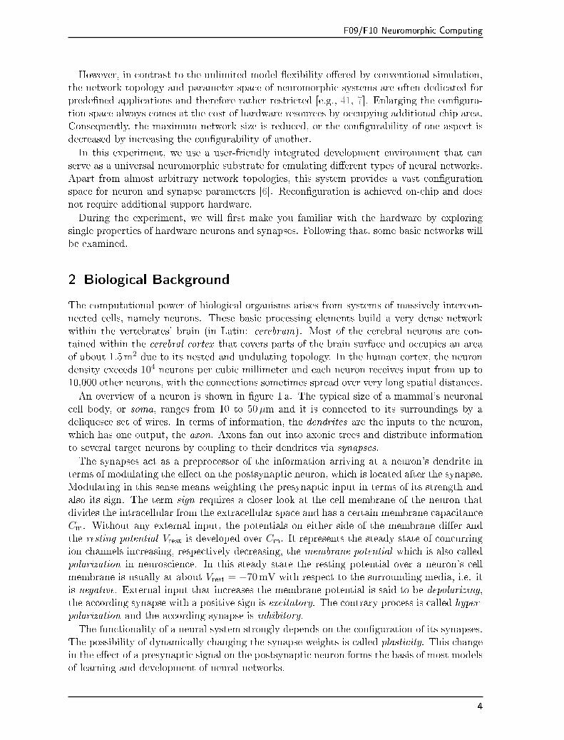
The computational power of biological organisms arises from systems of massively intercon-nected cells, namely neurons. These basic processing elements build a very dense networkwithin the vertebrates' brain (in Latin: cerebrum). Most of the cerebral neurons are con-tained within the cerebral cortex that covers parts of the brain surface and occupies an areaof about 1.5m2 due to its nested and undulating topology. In the human cortex, the neurondensity exceeds 104 neurons per cubic millimeter and each neuron receives input from up to10,000 other neurons, with the connections sometimes spread over very long spatial distances.

An overview of a neuron is shown in �gure 1 a. The typical size of a mammal's neuronalcell body, or soma, ranges from 10 to 50µm and it is connected to its surroundings by adeliquesce set of wires. In terms of information, the dendrites are the inputs to the neuron,which has one output, the axon. Axons fan out into axonic trees and distribute informationto several target neurons by coupling to their dendrites via synapses.

The synapses act as a preprocessor of the information arriving at a neuron's dendrite interms of modulating the e�ect on the postsynaptic neuron, which is located after the synapse.Modulating in this sense means weighting the presynaptic input in terms of its strength andalso its sign. The term sign requires a closer look at the cell membrane of the neuron thatdivides the intracellular from the extracellular space and has a certain membrane capacitanceCm. Without any external input, the potentials on either side of the membrane di�er andthe resting potential Vrest is developed over Cm. It represents the steady state of concurringion channels increasing, respectively decreasing, the membrane potential which is also calledpolarization in neuroscience. In this steady state the resting potential over a neuron's cellmembrane is usually at about Vrest = −70 mV with respect to the surrounding media, i.e. itis negative. External input that increases the membrane potential is said to be depolarizing,the according synapse with a positive sign is excitatory. The contrary process is called hyper-polarization and the according synapse is inhibitory.

The functionality of a neural system strongly depends on the con�guration of its synapses.The possibility of dynamically changing the synapse weights is called plasticity. This changein the e�ect of a presynaptic signal on the postsynaptic neuron forms the basis of most modelsof learning and development of neural networks.

4


a) b)

t1

(f2)t1

(f1)

t2

(f2)t2

(f1)

Vrest

V(t)

q

A

B

t

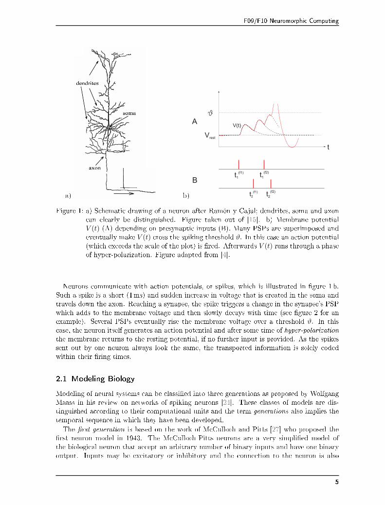
Figure 1: a) Schematic drawing of a neuron after Ramón y Cajal; dendrites, soma and axoncan clearly be distinguished. Figure taken out of [15]. b) Membrane potentialV (t) (A) depending on presynaptic inputs (B). Many PSPs are superimposed andeventually make V (t) cross the spiking threshold ϑ. In this case an action potential(which exceeds the scale of the plot) is �red. Afterwards V (t) runs through a phaseof hyper-polarization. Figure adapted from [4].

Neurons communicate with action potentials, or spikes, which is illustrated in �gure 1 b.Such a spike is a short (1ms) and sudden increase in voltage that is created in the soma andtravels down the axon. Reaching a synapse, the spike triggers a change in the synapse's PSPwhich adds to the membrane voltage and then slowly decays with time (see �gure 2 for anexample). Several PSPs eventually rise the membrane voltage over a threshold ϑ. In thiscase, the neuron itself generates an action potential and after some time of hyper-polarizationthe membrane returns to the resting potential, if no further input is provided. As the spikessent out by one neuron always look the same, the transported information is solely codedwithin their �ring times.

2.1 Modeling Biology

Modeling of neural systems can be classi�ed into three generations as proposed by WolfgangMaass in his review on networks of spiking neurons [24]. These classes of models are dis-tinguished according to their computational units and the term generations also implies thetemporal sequence in which they have been developed.

The �rst generation is based on the work of McCulloch and Pitts [27] who proposed the�rst neuron model in 1943. The McCulloch-Pitts neurons are a very simpli�ed model ofthe biological neuron that accept an arbitrary number of binary inputs and have one binaryoutput. Inputs may be excitatory or inhibitory and the connection to the neuron is also

5


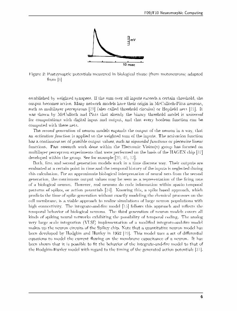
Figure 2: Postsynaptic potentials measured in biological tissue (from motoneurons; adaptedfrom [8]

established by weighted synapses. If the sum over all inputs exceeds a certain threshold, theoutput becomes active. Many network models have their origin in McCulloch-Pitts neurons,such as multilayer perceptrons [29] (also called threshold circuits) or Hop�eld nets [21]. Itwas shown by McCulloch and Pitts that already the binary threshold model is universalfor computations with digital input and output, and that every boolean function can becomputed with these nets.The second generation of neuron models expands the output of the neuron in a way, that

an activation function is applied to the weighted sum of the inputs. The activation functionhas a continuous set of possible output values, such as sigmoidal functions or piecewise linearfunctions. Past research work done within the Electronic Vision(s) group has focused onmultilayer perceptron experiments that were performed on the basis of the HAGEN chip [37]developed within the group. See for example [20, 40, 13].Both, �rst and second generation models work in a time discrete way. Their outputs are

evaluated at a certain point in time and the temporal history of the inputs is neglected duringthis calculation. For an approximate biological interpretation of neural nets from the secondgeneration, the continuous output values may be seen as a representation of the �ring rateof a biological neuron. However, real neurons do code information within spatio-temporalpatterns of spikes, or action potentials [24]. Knowing this, a spike-based approach, whichpredicts the time of spike generation without exactly modeling the chemical processes on thecell membrane, is a viable approach to realize simulations of large neuron populations withhigh connectivity. The integrate-and-�re model [15] follows this approach and re�ects thetemporal behavior of biological neurons. The third generation of neuron models covers allkinds of spiking neural networks exhibiting the possibility of temporal coding. The analogvery large scale integration (VLSI) implementation of a modi�ed integrate-and-�re modelmakes up the neuron circuits of the Spikey chip. Note that a quantitative neuron model hasbeen developed by Hodgkin and Huxley in 1952 [19]. This model uses a set of di�erentialequations to model the current �owing on the membrane capacitance of a neuron. It hasbeen shown that it is possible to �t the behavior of the integrate-and-�re model to that ofthe Hodgkin-Huxley model with regard to the timing of the generated action potentials [31].

6


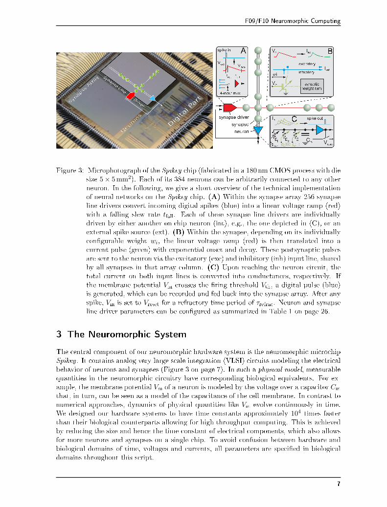
Figure 3: Microphotograph of the Spikey chip (fabricated in a 180 nm CMOS process with diesize 5 × 5 mm2). Each of its 384 neurons can be arbitrarily connected to any otherneuron. In the following, we give a short overview of the technical implementationof neural networks on the Spikey chip. (A) Within the synapse array 256 synapseline drivers convert incoming digital spikes (blue) into a linear voltage ramp (red)with a falling slew rate tfall. Each of these synapse line drivers are individuallydriven by either another on-chip neuron (int), e.g., the one depicted in (C), or anexternal spike source (ext). (B) Within the synapse, depending on its individuallycon�gurable weight wi, the linear voltage ramp (red) is then translated into acurrent pulse (green) with exponential onset and decay. These postsynaptic pulsesare sent to the neuron via the excitatory (exc) and inhibitory (inh) input line, sharedby all synapses in that array column. (C) Upon reaching the neuron circuit, thetotal current on both input lines is converted into conductances, respectively. Ifthe membrane potential Vm crosses the �ring threshold Vth, a digital pulse (blue)is generated, which can be recorded and fed back into the synapse array. After anyspike, Vm is set to Vreset for a refractory time period of τrefrac. Neuron and synapseline driver parameters can be con�gured as summarized in Table 1 on page 26.

3 The Neuromorphic System

The central component of our neuromorphic hardware system is the neuromorphic microchipSpikey . It contains analog very-large-scale integration (VLSI) circuits modeling the electricalbehavior of neurons and synapses (Figure 3 on page 7). In such a physical model, measurablequantities in the neuromorphic circuitry have corresponding biological equivalents. For ex-ample, the membrane potential Vm of a neuron is modeled by the voltage over a capacitor Cm

that, in turn, can be seen as a model of the capacitance of the cell membrane. In contrast tonumerical approaches, dynamics of physical quantities like Vm evolve continuously in time.We designed our hardware systems to have time constants approximately 104 times fasterthan their biological counterparts allowing for high-throughput computing. This is achievedby reducing the size and hence the time constant of electrical components, which also allowsfor more neurons and synapses on a single chip. To avoid confusion between hardware andbiological domains of time, voltages and currents, all parameters are speci�ed in biologicaldomains throughout this script.

7


3.1 The Neuromorphic Chip

On Spikey (Figure 3 on page 7), a VLSI version of the standard leaky integrate-and-�re (LIF)neuron model with conductance-based synapses is implemented [11]:

Cm

dV

dt= gleak (V − El) +

∑j

gj(t) (V − Ex) +∑k

gk(t) (V − Ei) (1)

For details on its hardware implementation see Figure 3 on page 7, [36] and [22]. Theconstant Cm represents the total membrane capacitance. Thus the current �owing on themembrane is modeled multiplying the derivative of the membrane voltage V with Cm. Theconductance gleak models the ion channels that pull the membrane voltage towards the leakagereversal potential1 El. The membrane �nally will reach this potential, if no other input ispresent. Excitatory and inhibitory ion channels are modeled by synapses connected to theexcitatory and the inhibitory reversal potentials Ex and Ei respectively. By summing overj, all excitatory synapses are covered by the �rst sum. The index k runs over all inhibitorysynapses in the second sum.

The time course of the synaptic activation is modeled as a product of the synaptic weightwj,k(t) and a maximum conductance gmax

j,k (t):

gj,k(t) = pj,k(t) · wj,k(t) · gmaxj,k (t) (2)

where the time course pj,k(t) of synaptic conductances is a linear transformation of the currentpulses shown in Figure 3 on page 7 (green), and hence an exponentially decaying function oftime.

Plasticity is included in the model by varying wj,k and gmaxj,k with time. Since the involved

time-scales vary greatly between short-term and longterm plasticity, both mechanisms act atdi�erent stages of the synaptic signal transmission chain. The weights wj,k are used for theinitial setup of the connection strengths. They are modi�ed by the implemented long-termplasticity algorithm spike timing dependent plasticity (STDP) and thus vary slowly withtime t (in case STDP is enabled for the actual experiment). Shortterm plasticity acts bytemporarily increasing or decreasing the maximum conductance gmax

j,k .

The propagation of spikes within the Spikey chip is illustrated in Figure 3 on page 7 anddescribed in detail by [36]. Spikes enter the chip as time-stamped events using standard digitalsignaling techniques that facilitate long-range communication, e.g., to the host computer orother chips. Such digital packets are processed in discrete time in the digital part of the chip,where they are transformed into digital pulses entering the synapse line driver (blue in Figure3 on page 7A). These pulses propagate in continuous time between on-chip neurons, and areoptionally transformed back into digital spike packets for o�-chip communication.

3.1.1 Short Term Plasticity (STP)

The strength of a synaptic connection (also called synaptic e�cacy) has been shown to changewith presynaptic activity on the time scale of hundred milliseconds [44]. The hardware im-plementation of such short-term plasticity is close to the model introduced by [43]. However,

1The reversal potential of a particular ion is the membrane voltage at which there is no net �ow of ions

from one side of the membrane to the other. The membrane voltage is pulled towards this potential if the

according ion channel becomes active.

8


on hardware STP can either be depressing or facilitating, but not mixtures of both as allowedby the original model.

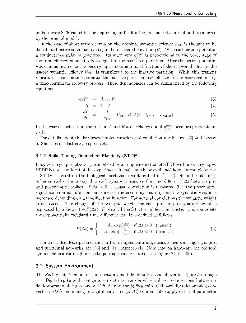
In the case of short term depression the absolute synaptic e�cacy ASE is thought to bedistributed between an inactive (I) and a recovered partition (R). With each action potentiala conductance pulse is generated. Its maximum gmax

j,k is proportional to the percentage ofthe total e�cacy momentarily assigned to the recovered partition. After the action potentialwas communicated to the post-synaptic neuron a �xed fraction of the recovered e�cacy, theusable synaptic e�cacy USE, is transferred to the inactive partition. While this transferrepeats with each action potential the inactive partition loses e�cacy to the recovered one bya time-continuous recovery process. These dependencies can be summarized by the followingequations:

gmaxj,k = ASE ·R (3)

R = 1 − I (4)

dI

dt= − I

τrec+ USE ·R · δ(t− taction potential) (5)

In the case of facilitation the roles of I and R are exchanged and gmaxj,k becomes proportional

to I.

For details about the hardware implementation and emulation results, see [39] and Lesson5: Short-term plasticity, respectively.

3.1.2 Spike Timing Dependent Plasticity (STDP)

Long term synaptic plasticity is modeled by an implementation of STDP within each synapse.STDP is not a supbject of this experiment, it shall shortly be explained here, for completeness:

STDP is based on the biological mechanism as described in [1, 42]. Synaptic plasticityis herein realized in a way that each synapse measures the time di�erence ∆t between pre-and postsynaptic spikes. If ∆t > 0, a causal correlation is measured (i.e. the presynapticsignal contributed to an output spike of the according neuron) and the synaptic weight isincreased depending on a modi�cation function. For acausal correlations the synaptic weightis decreased. The change of the synaptic weight for each pre- or postsynaptic signal isexpressed by a factor 1 + F (∆t). F is called the STDP modi�cation function and representsthe exponentially weighted time di�erence ∆t. It is de�ned as follows:

F (∆t) =

{A+ exp(∆t

τ+) if ∆t > 0 (causal)

−A− exp(−∆tτ−

) if ∆t < 0 (acausal)(6)

For a detailed description of the hardware implementation, measurements of single synapsesand functional networks, see [36] and [34], respectively. Note that on hardware the reducedsymmetric nearest neighbor spike pairing scheme is used (see Figure 7C in [30]).

3.2 System Environment

The Spikey chip is mounted on a network module described and shown in Figure 5 on page11. Digital spike and con�guration data is transferred via direct connections between a�eld-programmable gate array (FPGA) and the Spikey chip. Onboard digital-to-analog con-verter (DAC) and analog-to-digital converter (ADC) components supply external parameter

9


a) b)

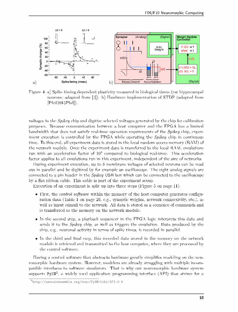
Figure 4: a) Spike-timing dependent plasticity measured in biological tissue (rat hippocampalneurons; adapted from [2]). b) Hardware implementation of STDP (adapted from[Pfeil2015Phd]).

voltages to the Spikey chip and digitize selected voltages generated by the chip for calibrationpurposes. Because communication between a host computer and the FPGA has a limitedbandwidth that does not satisfy real-time operation requirements of the Spikey chip, exper-iment execution is controlled by the FPGA while operating the Spikey chip in continuoustime. To this end, all experiment data is stored in the local random access memory (RAM) ofthe network module. Once the experiment data is transferred to the local RAM, emulationsrun with an acceleration factor of 104 compared to biological real-time. This accelerationfactor applies to all emulations run in this experiment, independent of the size of networks.During experiment execution, up to 8 membrane voltages of selected neurons can be read

out in parallel and be digitized by for example an oscilloscope. The eight analog signals areconnected to a pin header in the Spikey USB box which can be connected to the oscilloscopeby a �at ribbon cable. This cable is part of the experiment setup.Execution of an experiment is split up into three steps (Figure 5 on page 11).

• First, the control software within the memory of the host computer generates con�gu-ration data (Table 1 on page 26, e.g., synaptic weights, network connectivity, etc.), aswell as input stimuli to the network. All data is stored as a sequence of commands andis transferred to the memory on the network module.

• In the second step, a playback sequencer in the FPGA logic interprets this data andsends it to the Spikey chip, as well as triggers the emulation. Data produced by thechip, e.g., neuronal activity in terms of spike times, is recorded in parallel.

• In the third and �nal step, this recorded data stored in the memory on the networkmodule is retrieved and transmitted to the host computer, where they are processed bythe control software.

Having a control software that abstracts hardware greatly simpli�es modeling on the neu-romorphic hardware system. However, modelers are already struggling with multiple incom-patible interfaces to software simulators. That is why our neuromorphic hardware systemsupports PyNN2, a widely used application programming interface (API) that strives for a

2http://neuralensemble.org/trac/PyNN/wiki/API-0.6

10

http://neuralensemble.org/trac/PyNN/wiki/API-0.6


Network Module

RAMSequencer

DAC/ADC

Neuromorphic Network

Host Computer

ControlSoftware

PyNN

Spikey Chip

(FPGA)

(neuronal networkmodeling language)

Oscilloscope

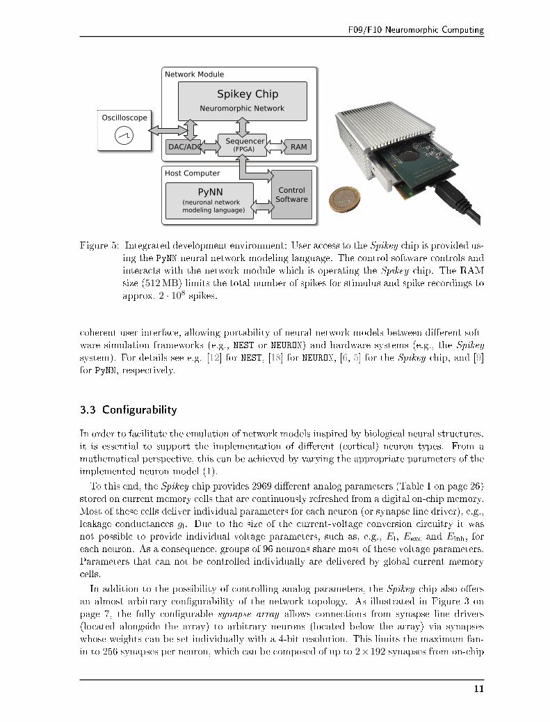
Figure 5: Integrated development environment: User access to the Spikey chip is provided us-ing the PyNN neural network modeling language. The control software controls andinteracts with the network module which is operating the Spikey chip. The RAMsize (512 MB) limits the total number of spikes for stimulus and spike recordings toapprox. 2 · 108 spikes.

coherent user interface, allowing portability of neural network models between di�erent soft-ware simulation frameworks (e.g., NEST or NEURON) and hardware systems (e.g., the Spikeysystem). For details see e.g. [12] for NEST, [18] for NEURON, [6, 5] for the Spikey chip, and [9]for PyNN, respectively.

3.3 Con�gurability

In order to facilitate the emulation of network models inspired by biological neural structures,it is essential to support the implementation of di�erent (cortical) neuron types. From amathematical perspective, this can be achieved by varying the appropriate parameters of theimplemented neuron model (1).

To this end, the Spikey chip provides 2969 di�erent analog parameters (Table 1 on page 26)stored on current memory cells that are continuously refreshed from a digital on-chip memory.Most of these cells deliver individual parameters for each neuron (or synapse line driver), e.g.,leakage conductances gl. Due to the size of the current-voltage conversion circuitry it wasnot possible to provide individual voltage parameters, such as, e.g., El, Eexc and Einh, foreach neuron. As a consequence, groups of 96 neurons share most of these voltage parameters.Parameters that can not be controlled individually are delivered by global current memorycells.

In addition to the possibility of controlling analog parameters, the Spikey chip also o�ersan almost arbitrary con�gurability of the network topology. As illustrated in Figure 3 onpage 7, the fully con�gurable synapse array allows connections from synapse line drivers(located alongside the array) to arbitrary neurons (located below the array) via synapseswhose weights can be set individually with a 4-bit resolution. This limits the maximum fan-in to 256 synapses per neuron, which can be composed of up to 2×192 synapses from on-chip

11


neurons3, and up to 256 synapses from external spike sources. Because the total number ofneurons exceeds the number of inputs per neuron, an all-to-all connectivity is not possible.For all networks indroduced in this experiment, the connection density is much lower thanrealizable on the chip, which supports the chosen trade-o� between inputs per neuron andtotal neuron count.

3.4 Calibration

Device mismatch that arises from hardware production variability causes �xed-pattern noise,which causes parameters to vary from neuron to neuron as well as from synapse to synapse.Electronic noise (including thermal noise) also a�ects dynamic variables, as, e.g., the mem-brane potential Vm. Consequently, experiments will exhibit some amount of both neuron-to-neuron and trial-to-trial variability given the same input stimulus. It is, however, importantto note that these types of variations are not unlike the neuron diversity and response stochas-ticity found in biology [17, 25, 26, 35].

To facilitate modeling and provide repeatability of experiments on arbitrary Spikey chips, itis essential to minimize these e�ects by calibration routines. Many calibrations have directlycorresponding biological model parameters, e.g., membrane time constants (described in thefollowing), �ring thresholds, synaptic e�cacies or PSP shapes. Others have no equivalents,like compensations for shared parameters or workarounds of defects [e.g., 23, 3, 34]. In general,calibration results are used to improve the mapping between biological input parameters andthe corresponding target hardware voltages and currents, as well as to determine the dynamicrange of all model parameters [e.g., 5].

3.4.1 Calibration of Membrane Time Constant

While the calibration of most parameters is rather technical, but straightforward (e.g., allneuron voltage parameters), some require more elaborate techniques. These include thecalibration of τm, STP as well as synapse line drivers and some more which are not relevantfor this experiment. The membrane time constant4 τm = Cm/gl di�ers from neuron toneuron mostly due to variations in the leakage conductance gl. However, gl is independentlyadjustable for every neuron. Because this conductance is not directly measurable, an indirectcalibration method is employed. To this end, the threshold potential Vth is set below theresting potential El. As a consequence, the membrane potential would get pulled above thethreshold potential only through the leakage mechanism (no synaptic input), if there was nospiking mechanism present. E�ectively, a spike is triggered as soon as the threshold potentialis reached. Following each spike, the membrane potential is clamped to Vreset for an absoluterefractory time τrefrac, after which it evolves exponentially towards the resting potential El

until the threshold voltage triggers a spike and the next cycle begins. If the threshold voltageis set to Vth = El − 1/e · (El − Vreset), the spike frequency equals 1/(τm + τrefrac), therebyallowing an indirect measurement and calibration of gl and therefore τm. For a given τmand τrefrac = const, Vth can be calculated. An iterative method is applied to �nd the best-matching Vth, because the exact hardware values for El, Vreset and Vth are only known after

3The chip contains two identical synapse arrays, each driving 192 neurons. Neurons from both halves can

drive a synapse driver.4The membrane voltage eventually decays to its resting potential with this RC time constant when no other

input to the neuron is present.

12


10 80τm[ms]0

150neu

rons

10 80τm[ms]0

150

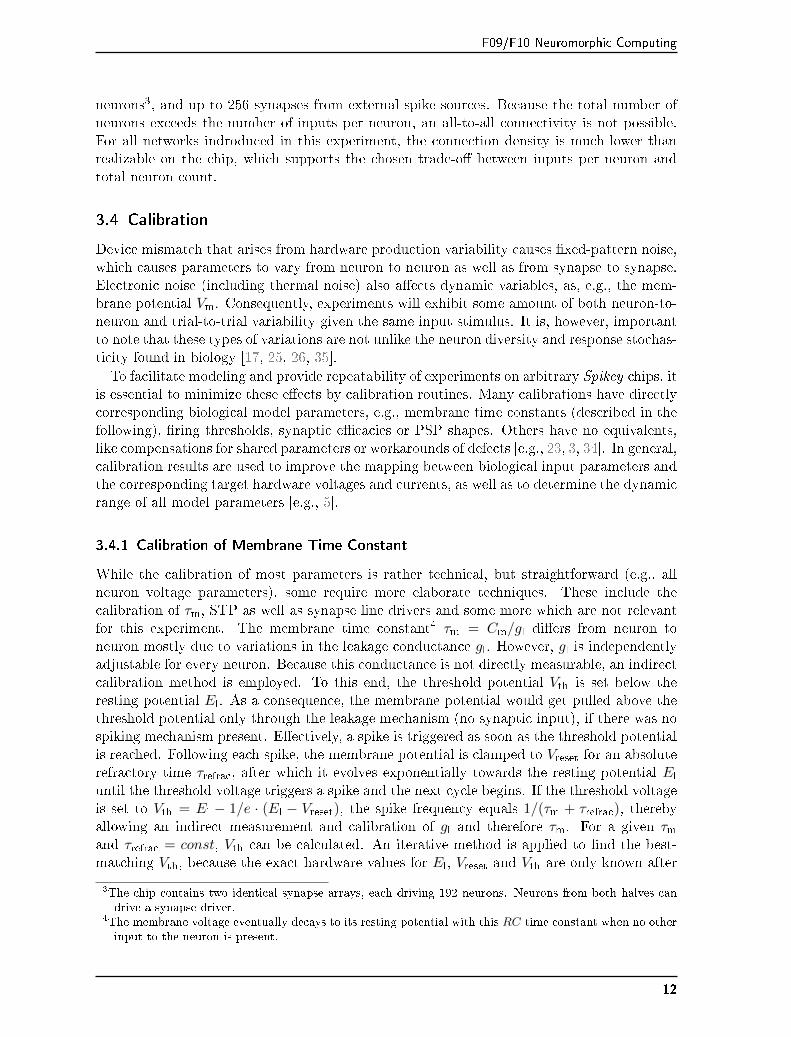
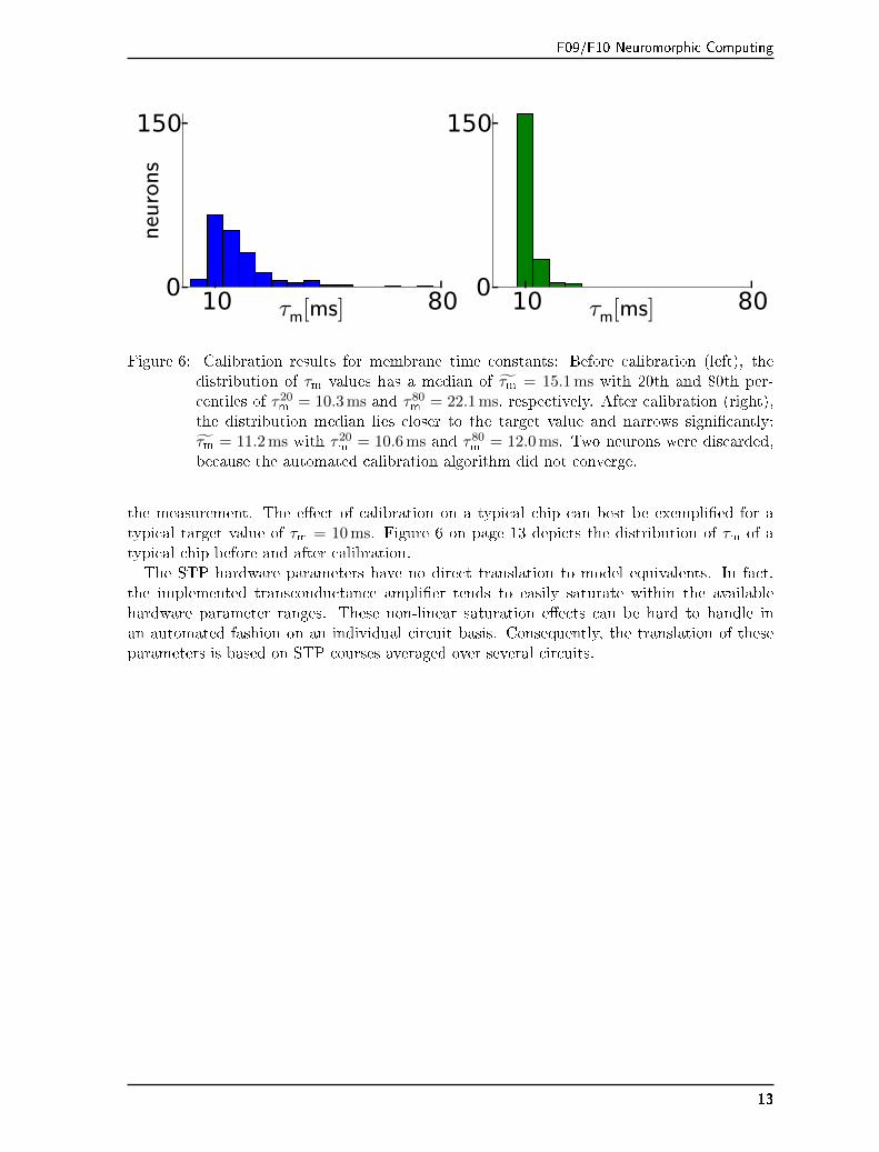
Figure 6: Calibration results for membrane time constants: Before calibration (left), thedistribution of τm values has a median of τ̃m = 15.1 ms with 20th and 80th per-centiles of τ20

m = 10.3 ms and τ80m = 22.1 ms, respectively. After calibration (right),

the distribution median lies closer to the target value and narrows signi�cantly:τ̃m = 11.2 ms with τ20

m = 10.6 ms and τ80m = 12.0 ms. Two neurons were discarded,

because the automated calibration algorithm did not converge.

the measurement. The e�ect of calibration on a typical chip can best be exempli�ed for atypical target value of τm = 10 ms. Figure 6 on page 13 depicts the distribution of τm of atypical chip before and after calibration.The STP hardware parameters have no direct translation to model equivalents. In fact,

the implemented transconductance ampli�er tends to easily saturate within the availablehardware parameter ranges. These non-linear saturation e�ects can be hard to handle inan automated fashion on an individual circuit basis. Consequently, the translation of theseparameters is based on STP courses averaged over several circuits.

13


4 Experiments

4.1 Investigating a Single Neuron

During this task you will learn how to use the Spikey neuromophic chip, and how to recordrelevant analog quantities with an oscilloscope, as well as with an analog-to-digital converter(ADC) that is available in the system.

Before you start, make yourself familiar with the hardware setup and establish the necces-sary connections (ask your supervisor in case anything should be unclear!):

• If not set up, connect all peripherals to the Intel NUC computer and put it on yourdesk. All tasks will be run from this computer.

• Connect the Aluminum box with the Spikey chip to the USB hub, and the USB hub tothe Intel NUC computer.

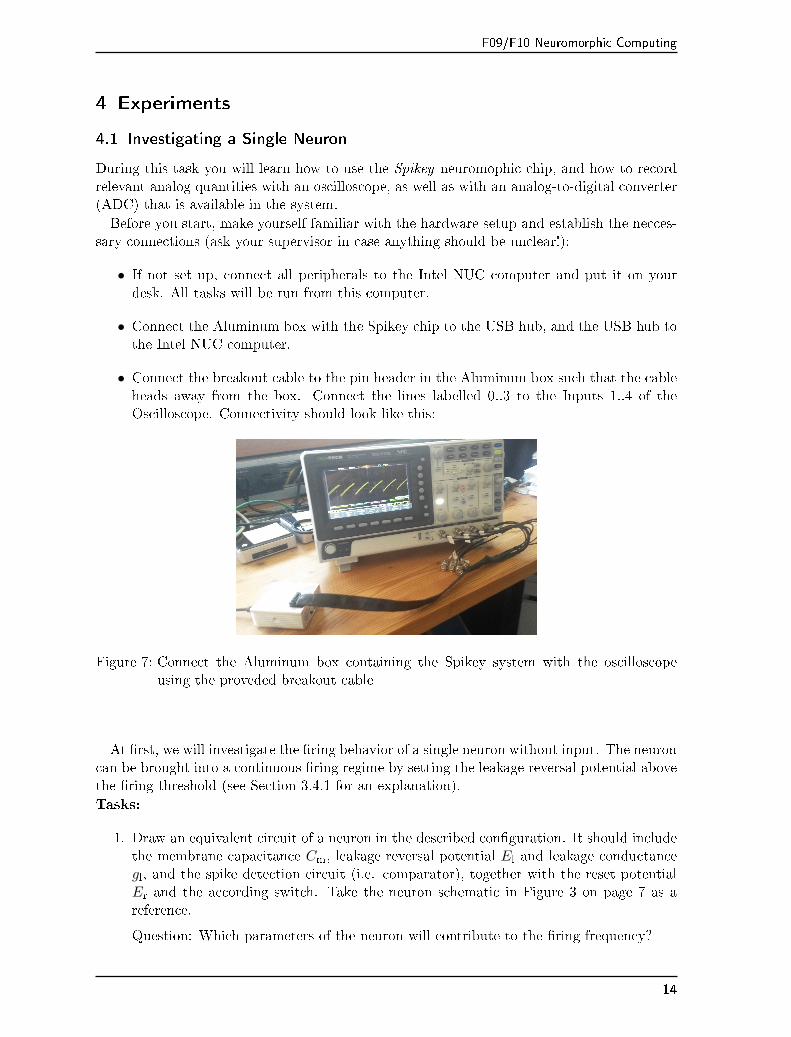
• Connect the breakout cable to the pin header in the Aluminum box such that the cableheads away from the box. Connect the lines labelled 0..3 to the Inputs 1..4 of theOscilloscope. Connectivity should look like this:

Figure 7: Connect the Aluminum box containing the Spikey system with the oscilloscopeusing the proveded breakout cable

At �rst, we will investigate the �ring behavior of a single neuron without input. The neuroncan be brought into a continuous �ring regime by setting the leakage reversal potential abovethe �ring threshold (see Section 3.4.1 for an explanation).

Tasks:

1. Draw an equivalent circuit of a neuron in the described con�guration. It should includethe membrane capacitance Cm, leakage reversal potential El and leakage conductancegl, and the spike detection circuit (i.e. comparator), together with the reset potentialEr and the according switch. Take the neuron schematic in Figure 3 on page 7 as areference.

Question: Which parameters of the neuron will contribute to the �ring frequency?

14


2. Power up the NUC and the Spikey USB port. Graphically log on to the NUC (askyour supervisor for credentials). Open a terminal - all experiments will be run from thecommand line.

3. The �rst step of usage is to run a very simple PyNN script which con�gures a single neuronwith the aforementioned parameters � the resting potential is already con�gured to belarger than the threshold potential.

In your user's home directory, change to the directory fp-spikey. First open the scriptin an editor of your choice. Geany is a good choice if you like to use a GUI. Note: The'&' at the end of the command line lets you use the command line after starting geany.

<host-name>:< > geany experiments/fp_task1_1membrane.py &

Then, run the script (nothing particular will happen, besides some status output onthe terminal).

<host-name>:< > python experiments/fp_task1_1membrane.py

The script will con�gure one neuron with the described parameters and connects itsoutput to the analog readout lines. The analog signal will be digitized by the onboardADC using the commandspynn.record_v(neuron[0], �) andmembrane = pynn.membraneOutput,the latter transferring the digitized membrane data into the numpy array membrane.The script also contains example code to plot the membrane voltage trace into the �lefp_task1_1membrane.png.

In the generated plot, verify that the values for threshold voltage Vth and reset voltageEr are set correctly.

4. In parallel, the membrane can be observed on the oscilloscope. Make yourself familiarwith the usage of the oscilloscope and display the membrane voltage output of thecon�gured neuron on channel 1. Determine the average �ring rate of the neuron andits standard deviation using the measure and statistics function of the oscilloscope.

Calculate the mean �ring rate of the spikes received in the spikes array and comparewith the oscilloscope measurement. Verify the temporal acceleration factor between thex-axis of the generated plot and the oscilloscope's time axis.

Hint: To obtain a distribution of the interspike intervals (ISIs), you can calculate thepair-wise di�erence of the received spike times and store them in a new array. Themean value of these di�erences and its standard deviation can be calculated with theaccording NumPy functions.

15


4.2 Calibrating Neuron Parameters

You will already have recognized that the �ring rate of the neuron is not constant, which alsomanifests in a potentially rather large standard deviation of the mean �ring rate (about 10%).This is due to temporal noise, whereas the variation of �ring rates between several di�erentneurons on the chip is caused by �xed pattern noise: Fixed-pattern noise are variationsof neuron and synapse parameters across the chip due to imperfections in the productionprocess. Calibration can reduce this noise, because it is approximately constant over time.In contrast, temporal noise, including electronic noise and temperature �uctuations, causesdi�erent results in consecutive emulations of identical networks.During this task you will investigate the variability of the hardware neurons' membrane

time constant τm = Cm/gl. It di�ers from neuron to neuron mostly due to variations in theleakage conductance gl. In order to investigate this, �rst connect the analog readout lines 0to 3 of the Spikey chip to channels 1 to 4 of the oscilloscope. The following scipt sets up 4identically con�gured neurons with parameters that would be valid for an experiment.

<host-name>:<~> python networks/fp_task2_calib4membranes.py

Tasks:

1. Calculate the new �ring threshold voltage Vth to bring these neurons into a continuous�ring regime for measuring the membrane time constant τm, using this equation:

Vth = El − 1/e · (El − Vreset)

Given this Vth, a �ring rate of 1/(τm+τrefrac) is expected. Explain why (in your report).The script already contains valid neuron parameters; according to these parameters,calculate the expected �ring rate.

Note: The PyNN-default parameters of the neuron model can be obtained in an interac-tive Python shell (use e.g. ipython) by typing pynn.IF_facets_hardware1.default_parametersafter an import pyNN.hardware.spikey as pynn. You can use this as a reference tosee how much you probably deviate from the default.

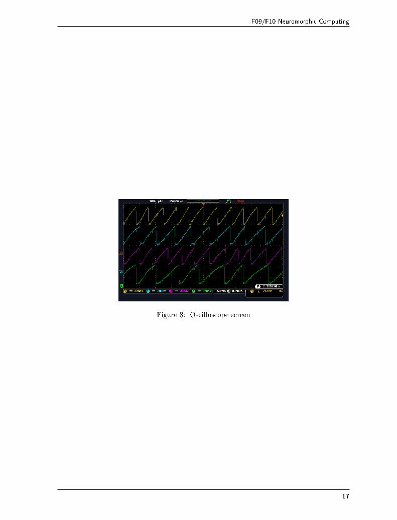
2. Change the setting for Vth in the script accordingly and run the script. Adjust theoscilloscope recording in a way that all 4 membrane voltages can be seen. It shouldlook like this:

Use the measurement functions of the oscilloscope to simultaneously measure the �ringfrequency of the four connected neurons. Enable the statistics function to have theoscilloscope calculate mean values and standard deviation.

3. Calibrate these neurons for identical �ring rate, thus identical membrane time constant,by adjusting the leak conductance gl for each neuron (note down the used values forgl). Explain possible reasons for the distribution of values (compare with the followingmeasurement):

4. Investigate the �xed-pattern noise across neurons: Record the �ring rates of severalneurons for the default value of the leak conductance (tipp: record all neurons at once).Interpret the distribution of these �ring rates by plotting a histogram and calculatingthe standard deviation. Compare with the plots in Figure 6 on page 13.

16


Figure 8: Oscilloscope screen

17


4.3 A Single Neuron with Synaptic Input

In this task, you will evaluate the in�uence of synaptic input to the neuron. A rather old,nevertheless valid, measurement of synaptic activity is shown in �gure 2. The displayed PSPshows a steep rise from a resting state and an exponential decay back to rest.In order to reproduce these measurements, stimulate one hardware neuron with a single

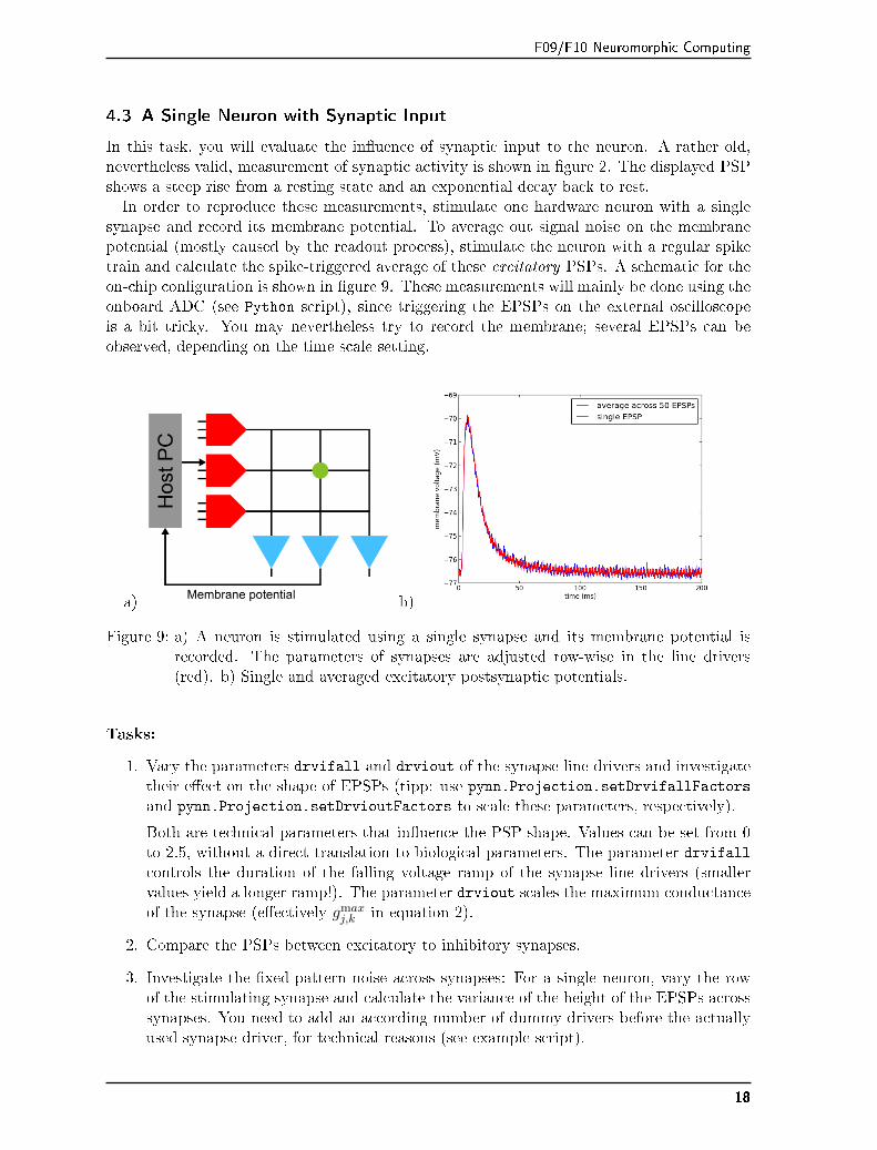
synapse and record its membrane potential. To average out signal noise on the membranepotential (mostly caused by the readout process), stimulate the neuron with a regular spiketrain and calculate the spike-triggered average of these excitatory PSPs. A schematic for theon-chip con�guration is shown in �gure 9. These measurements will mainly be done using theonboard ADC (see Python script), since triggering the EPSPs on the external oscilloscopeis a bit tricky. You may nevertheless try to record the membrane; several EPSPs can beobserved, depending on the time scale setting.

a) b)

Figure 9: a) A neuron is stimulated using a single synapse and its membrane potential isrecorded. The parameters of synapses are adjusted row-wise in the line drivers(red). b) Single and averaged excitatory postsynaptic potentials.

Tasks:

1. Vary the parameters drvifall and drviout of the synapse line drivers and investigatetheir e�ect on the shape of EPSPs (tipp: use pynn.Projection.setDrvifallFactorsand pynn.Projection.setDrvioutFactors to scale these parameters, respectively).

Both are technical parameters that in�uence the PSP shape. Values can be set from 0to 2.5, without a direct translation to biological parameters. The parameter drvifallcontrols the duration of the falling voltage ramp of the synapse line drivers (smallervalues yield a longer ramp!). The parameter drviout scales the maximum conductanceof the synapse (e�ectively gmax

j,k in equation 2).

2. Compare the PSPs between excitatory to inhibitory synapses.

3. Investigate the �xed-pattern noise across synapses: For a single neuron, vary the rowof the stimulating synapse and calculate the variance of the height of the EPSPs acrosssynapses. You need to add an according number of dummy drivers before the actuallyused synapse driver, for technical reasons (see example script).

18


In case of very noisy analog signals, you might need to apply a moving average to themembrane data (ask your supervisor).

4. In an additional script to this task (fp_task3_synin_epsp_stacked.py) you can �ndcommented lines for a di�erent stimulus generation. Use this stimulus to observe stackedEPSPs on the membrane, and reduce the temporal distance between the input spikesuntil the neuron �res at least once. Question: Qualitatively compare the relative heightsof the di�erent PSPs with the previous �xed-pattern noise results.

19


4.4 Short Term Plasticity

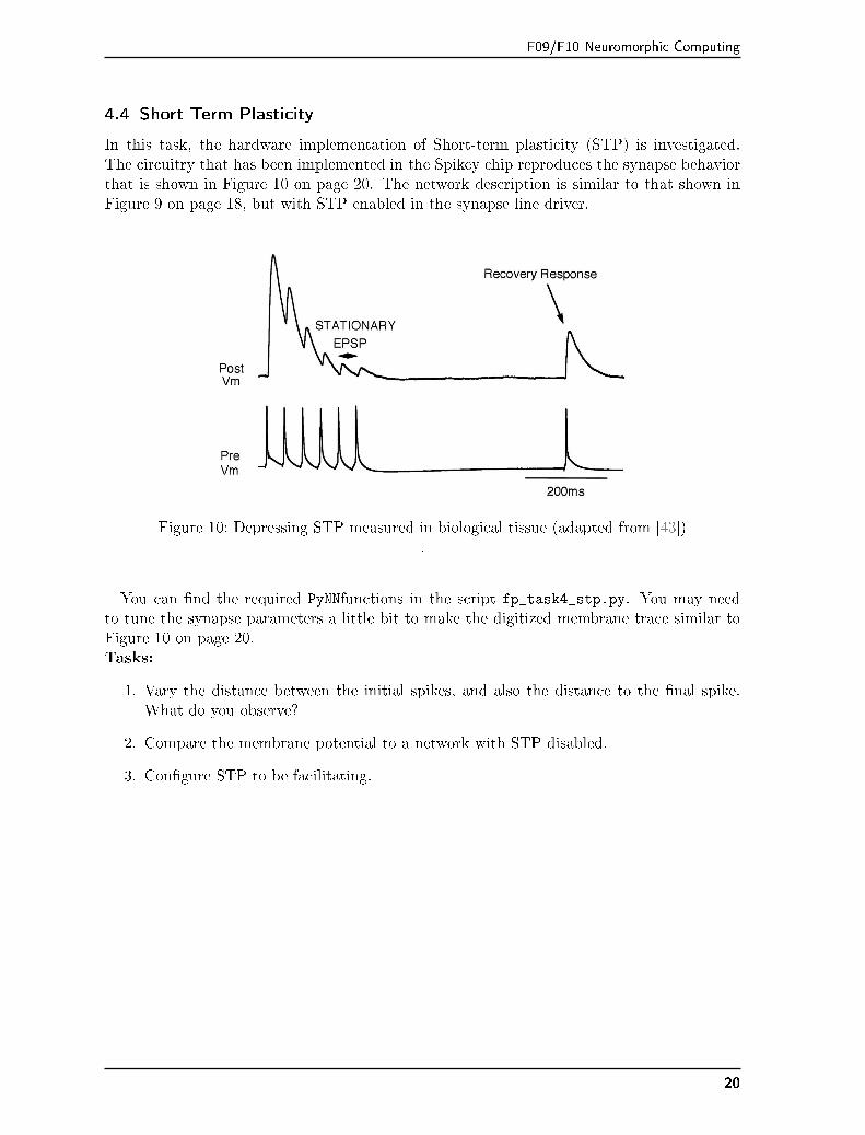
In this task, the hardware implementation of Short-term plasticity (STP) is investigated.The circuitry that has been implemented in the Spikey chip reproduces the synapse behaviorthat is shown in Figure 10 on page 20. The network description is similar to that shown inFigure 9 on page 18, but with STP enabled in the synapse line driver.

Figure 10: Depressing STP measured in biological tissue (adapted from [43]).

You can �nd the required PyNNfunctions in the script fp_task4_stp.py. You may needto tune the synapse parameters a little bit to make the digitized membrane trace similar toFigure 10 on page 20.Tasks:

1. Vary the distance between the initial spikes, and also the distance to the �nal spike.What do you observe?

2. Compare the membrane potential to a network with STP disabled.

3. Con�gure STP to be facilitating.

20


4.5 Feedforward Networks

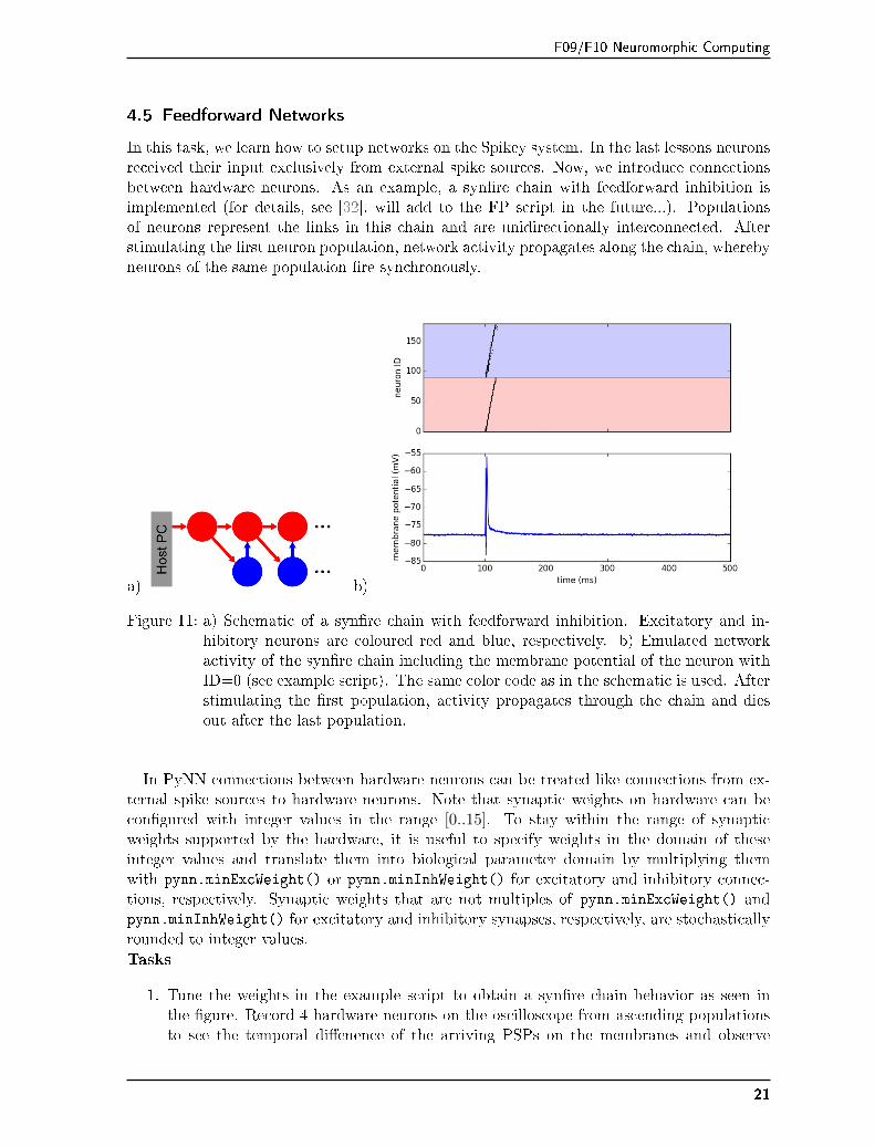
In this task, we learn how to setup networks on the Spikey system. In the last lessons neuronsreceived their input exclusively from external spike sources. Now, we introduce connectionsbetween hardware neurons. As an example, a syn�re chain with feedforward inhibition isimplemented (for details, see [32], will add to the FP script in the future...). Populationsof neurons represent the links in this chain and are unidirectionally interconnected. Afterstimulating the �rst neuron population, network activity propagates along the chain, wherebyneurons of the same population �re synchronously.

a) b)

Figure 11: a) Schematic of a syn�re chain with feedforward inhibition. Excitatory and in-hibitory neurons are coloured red and blue, respectively. b) Emulated networkactivity of the syn�re chain including the membrane potential of the neuron withID=0 (see example script). The same color code as in the schematic is used. Afterstimulating the �rst population, activity propagates through the chain and diesout after the last population.

In PyNN connections between hardware neurons can be treated like connections from ex-ternal spike sources to hardware neurons. Note that synaptic weights on hardware can becon�gured with integer values in the range [0..15]. To stay within the range of synapticweights supported by the hardware, it is useful to specify weights in the domain of theseinteger values and translate them into biological parameter domain by multiplying themwith pynn.minExcWeight() or pynn.minInhWeight() for excitatory and inhibitory connec-tions, respectively. Synaptic weights that are not multiples of pynn.minExcWeight() andpynn.minInhWeight() for excitatory and inhibitory synapses, respectively, are stochasticallyrounded to integer values.

Tasks

1. Tune the weights in the example script to obtain a syn�re chain behavior as seen inthe �gure. Record 4 hardware neurons on the oscilloscope from ascending populationsto see the temporal di�enence of the arriving PSPs on the membranes and observe

21


the timing of the arriving excitatory stimulus and the feedforward inhibition. Whathappens if you disable inhibition?

2. Reduce the number of neurons in each population and maximize the period of net-work activity. Which hardware feature limits the minimal number of neurons in eachpopulation?

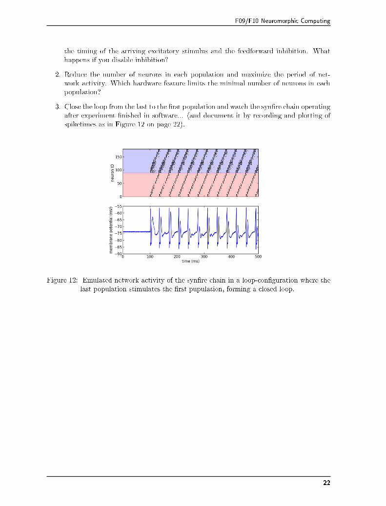
3. Close the loop from the last to the �rst population and watch the syn�re chain operatingafter experiment �nished in software... (and document it by recording and plotting ofspiketimes as in Figure 12 on page 22).

Figure 12: Emulated network activity of the syn�re chain in a loop-con�guration where thelast population stimulates the �rst pupulation, forming a closed loop.

22


4.6 Recurrent Networks

In this experiment, a recurrent network of neurons with sparse and random connections isinvestigated. The purpose of this network will be to add randomness to an otherwise regularlyspiking population of neurons. At �rst, you will set up a population of neurons that uses halfof the complete chip without any interconnect, similar to experiment 4.1:

• Set up a population of 192 neurons with standard parameters but the resting potential,e.g.: neuronParams = {'v_rest': -30.0} in order to have them in a regular �ringregime.

• Record the spike times of all 192 neurons and output the membrane voltage of 4 selectedneurons to the oscilloscope, for your "`visual"' reference. Verify that all neurons thatare displayed on the oscilloscope are �ring regularly.

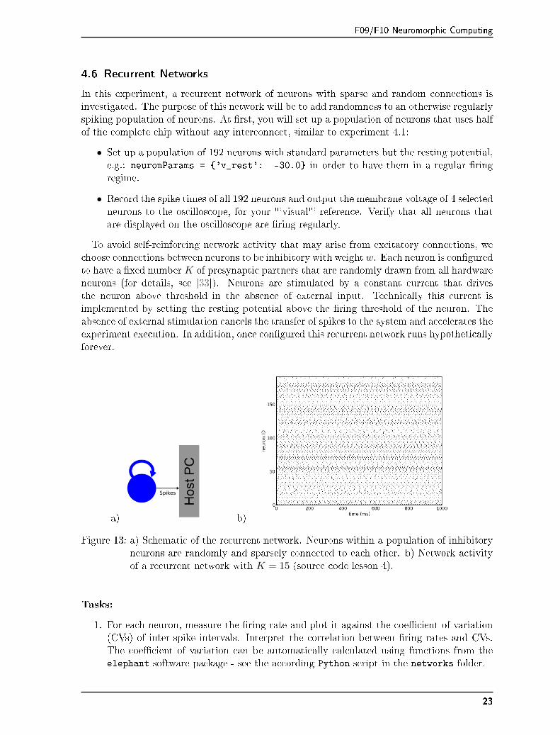
To avoid self-reinforcing network activity that may arise from excitatory connections, wechoose connections between neurons to be inhibitory with weight w. Each neuron is con�guredto have a �xed number K of presynaptic partners that are randomly drawn from all hardwareneurons (for details, see [33]). Neurons are stimulated by a constant current that drivesthe neuron above threshold in the absence of external input. Technically this current isimplemented by setting the resting potential above the �ring threshold of the neuron. Theabsence of external stimulation cancels the transfer of spikes to the system and accelerates theexperiment execution. In addition, once con�gured this recurrent network runs hypotheticallyforever.

a) b)

Figure 13: a) Schematic of the recurrent network. Neurons within a population of inhibitoryneurons are randomly and sparsely connected to each other. b) Network activityof a recurrent network with K = 15 (source code lesson 4).

Tasks:

1. For each neuron, measure the �ring rate and plot it against the coe�cient of variation(CVs) of inter-spike intervals. Interpret the correlation between �ring rates and CVs.The coe�cient of variation can be automatically calculated using functions from theelephant software package - see the according Python script in the networks folder.

23


2. Measure the dependence of the �ring rates and CVs on w and K by sweeping bothparameters in your script. You obtain a 2D-array of resuts that can be visualized e.g.by a color-coded 2d-plot.

Calibrate the network towards a �ring rate of approximately 25 Hz. Extra: And maxi-mize the average CV.

3. Long Evaluation: Calculate the pair-wise correlation between randomly drawn spiketrains of di�erent neurons in the network (again, consider using http://neuralensemble.org/elephant/ to calculate the correlation). Investigate the dependence of the averagecorrelation on w and K (tipp: use 100 pairs of neurons to calculate the average). Usethese results to minimize correlations in the activity of the network.

24

http://neuralensemble.org/elephant/

http://neuralensemble.org/elephant/


5 Acronyms

ADC analog-to-digital converter

DAC digital-to-analog converter

ISI interspike interval

PSP postsynaptic potential

STDP spike timing dependent plasticity

VLSI very large scale integration

25


6 Appendix

6.1 Relevant Technical Con�guration Parameters

Scope Name Type Description

Neuroncircuits (A)

n/a in Two digital con�guration bits activating the neuron and readout of its membranevoltage

gl in Bias current for neuron leakage circuitτrefrac in Bias current controlling neuron refractory timeEl sn Leakage reversal potentialEinh sn Inhibitory reversal potentialEexc sn Excitatory reversal potentialVth sn Firing threshold voltageVreset sn Reset potential

Synapse linedrivers (B)

n/a il Two digital con�guration bits selecting input of line drivern/a il Two digital con�guration bits setting line excitatory or inhibitory

trise, tfall il Two bias currents for rising and falling slew rate of presynaptic voltage rampgmaxi il Bias current controlling maximum voltage of presynaptic voltage ramp

Synapses (B) w is 4-bit weight of each individual synapse

STPrelated (C)

n/a il Two digital con�guration bits selecting short-term depression or facilitationUSE il Two digital con�guration bits tuning synaptic e�cacy for STPn/a sl Bias voltage controlling spike driver pulse length

τrec, τfacil sl Voltage controlling STP time constantI sl Short-term facilitation reference voltageR sl Short-term capacitor high potential

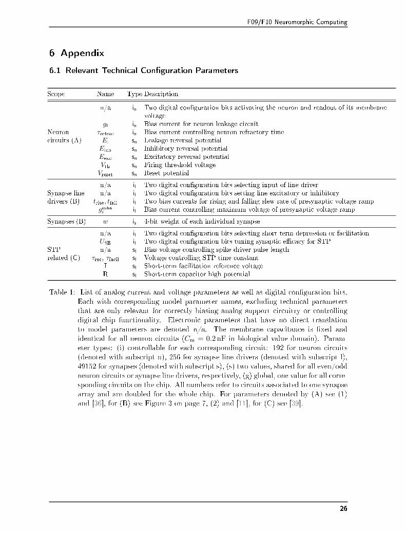
Table 1: List of analog current and voltage parameters as well as digital con�guration bits.Each with corresponding model parameter names, excluding technical parametersthat are only relevant for correctly biasing analog support circuitry or controllingdigital chip functionality. Electronic parameters that have no direct translationto model parameters are denoted n/a. The membrane capacitance is �xed andidentical for all neuron circuits (Cm = 0.2 nF in biological value domain). Param-eter types: (i) controllable for each corresponding circuit: 192 for neuron circuits(denoted with subscript n), 256 for synapse line drivers (denoted with subscript l),49152 for synapses (denoted with subscript s), (s) two values, shared for all even/oddneuron circuits or synapse line drivers, respectively, (g) global, one value for all corre-sponding circuits on the chip. All numbers refer to circuits associated to one synapsearray and are doubled for the whole chip. For parameters denoted by (A) see (1)and [36], for (B) see Figure 3 on page 7, (2) and [11], for (C) see [39].

26


References

[1] G. Bi and M. Poo. Synaptic modi�cations in cultured hippocampal neurons: Dependence onspike timing, synaptic strength, and postsynaptic cell type. Neural Computation, 9:503�514,1997.

[2] G. Bi and M. Poo. Synaptic modi�cation by correlated activity: Hebb's postulate revisited.24:139�66, 2001.

[3] Johannes Bill, Klaus Schuch, Daniel Brüderle, Johannes Schemmel, Wolfgang Maass, and Karl-heinz Meier. Compensating inhomogeneities of neuromorphic VLSI devices via short-term synap-tic plasticity. 4(129), 2010.

[4] Daniel Brüderle. Implementing spike-based computation on a hardware perceptron. Diplomathesis (English), University of Heidelberg, HD-KIP-04-16, 2004.

[5] Daniel Brüderle, Eric Müller, Andrew Davison, Eilif Muller, Johannes Schemmel, and Karl-heinz Meier. Establishing a novel modeling tool: A Python-based interface for a neuromorphichardware system. 3(17), 2009.

[6] Daniel Brüderle, Mihai Petrovici, Bernhard Vogginger, Matthias Ehrlich, Thomas Pfeil, Sebas-tian Millner, Andreas Grübl, Karsten Wendt, Eric Müller, Marc-Olivier Schwartz, Dan Hus-mann de Oliveira, Sebastian Jeltsch, Johannes Fieres, Moritz Schilling, Paul Müller, OliverBreitwieser, Venelin Petkov, Lyle Muller, Andrew P. Davison, Pradeep Krishnamurthy, JensKremkow, Mikael Lundqvist, Eilif Muller, Johannes Partzsch, Stefan Scholze, Lukas Zühl, AlainDestexhe, Markus Diesmann, Tobias C. Potjans, Anders Lansner, René Schü�ny, JohannesSchemmel, and Karlheinz Meier. A comprehensive work�ow for general-purpose neural mod-eling with highly con�gurable neuromorphic hardware systems. 104:263�296, 2011.

[7] E. Chicca, A. M. Whatley, P. Lichtsteiner, V. Dante, T. Delbruck, P. Del Giudice, R. J. Douglas,and G. Indiveri. A multichip pulse-based neuromorphic infrastructure and its application to amodel of orientation selectivity. 54(5):981�993, May 2007.

[8] J. S. Coombs, J. C. Eccles, and P. Fatt. Excitatory synaptic action in motoneurones. TheJournal of Physiology, 130(2):374�395, 1955.

[9] Andrew Davison, Eilif Muller, Daniel Brüderle, and Jens Kremkow. A common language forneuronal networks in software and hardware. The Neuromorphic Engineer, 2010.

[10] Andrew P. Davison, Eric Müller, Sebastian Schmitt, Bernhard Vogginger, David Lester, andThomas Pfeil. Hbp neuromorphic computing platform guidebook 0.1 - spikey school. Technicalreport, 2016.

[11] P. Dayan and L. F. Abbott. Theoretical Neuroscience. MIT Press, Cambridge, 2001.

[12] J. M. Eppler, M. Helias, E. Muller, M. Diesmann, and M. Gewaltig. PyNEST: a convenientinterface to the NEST simulator. 2:12, 2009.

[13] J. Fieres, J. Schemmel, and K. Meier. A convolutional neural network tolerant of synapticfaults for low-power analog hardware. In Proceedings of 2nd IAPR International Workshopon Arti�cialNeural Networks in Pattern Recognition (ANNPR 2006), Springer LectureNotes inArti�cial Intelligence, volume 4087, pages 122�132, 2006.

[14] S. Furber, D. Lester, L. Plana, J. Garside, E. Painkras, S. Temple, and A. Brown. Overview ofthe spinnaker system architecture. PP(99):1, 2012.

27


[15] Wulfram Gerstner and Werner Kistler. Spiking Neuron Models: Single Neurons, Populations,Plasticity. Cambridge University Press, 2002.

[16] Andreas Grübl. VLSI Implementation of a Spiking Neural Network. PhD thesis, Ruprecht-Karls-University, Heidelberg, 2007. Document No. HD-KIP 07-10.

[17] Anirudh Gupta, Yun Wang, and Henry Markram. Organizing principles for a diversity ofGABAergic interneurons and synapses in the neocortex. 287:273�278, 2000.

[18] Michael L. Hines, Andrew P. Davison, and Eilif Muller. NEURON and Python. Front. Neuroin-form., 2009.

[19] Alan Lloyd Hodgkin and Andrew F. Huxley. A quantitative description of membrane currentand its application to conduction and excitation in nerve. J Physiol, 117(4):500�544, August1952.

[20] Ste�en Hohmann. PhD thesis, University of Heidelberg, in preparation, 2005.

[21] J. J. Hop�eld. Neural networks and physical systems with emergent collective computationalabilities. Proceedings of the National Academy of Sciences, 79:2554�2558, 1982.

[22] Giacomo Indiveri, Bernabe Linares-Barranco, Tara Julia Hamilton, André van Schaik, RalphEtienne-Cummings, Tobi Delbruck, Shih-Chii Liu, Piotr Dudek, Philipp Hä�iger, Sylvie Renaud,Johannes Schemmel, Gert Cauwenberghs, John Arthur, Kai Hynna, Fopefolu Folowosele, SylvainSaighi, Teresa Serrano-Gotarredona, Jayawan Wijekoon, Yingxue Wang, and Kwabena Boahen.Neuromorphic silicon neuron circuits. 5(73), 2011.

[23] B. Kaplan, D. Brüderle, J. Schemmel, and K. Meier. High-conductance states on a neuromorphichardware system. In Proceedings of the 2009 International Joint Conference on Neural Networks(IJCNN), pages 1524�1530, Atlanta, june 2009. IEEE Press.

[24] W. Maass. Networks of spiking neurons: the third generation of neural network models. NeuralNetworks, 10:1659�1671, 1997.

[25] Wolfgang Maass, Thomas Natschläger, and Henry Markram. Real-time computing without stablestates: a new framwork for neural compuation based on perturbation. 14(11):2531�2560, 2002.

[26] Eve Marder and Jean-Marc Goaillard. Variability, compensation and homeostasis in neuron andnetwork function. 7(7):563�574, Jul 2006.

[27] Warren S. McCulloch and Walter Pitts. A logical calculus of the ideas immanent in nervousactivity. Bulletin of Mathematical Biophysics, pages 127�147, 1943.

[28] Carver Mead. Analog VLSI and neural systems. Addison-Wesley, Boston, MA, USA, 1989.

[29] Marvin Minsky and Seymour Papert. Perceptrons. MIT Press, Cambridge, MA, 1969.

[30] Abigail Morrison, Markus Diesmann, and Wulfram Gerstner. Phenomenological models of synap-tic plasticity based on spike timing. Biological Cybernetics, 98(6):459�478, June 2008.

[31] E. Mueller. Simulation of high-conductance states in cortical neural networks. Diploma thesis,University of Heidelberg, HD-KIP-03-22, 2003.

[32] Thomas Pfeil, Andreas Grübl, Sebastian Jeltsch, Eric Müller, Paul Müller, Mihai A. Petrovici,Michael Schmuker, Daniel Brüderle, Johannes Schemmel, and Karlheinz Meier. Six networks ona universal neuromorphic computing substrate. Frontiers in Neuroscience, 7:11, 2013.

28


[33] Thomas Pfeil, Jakob Jordan, Tom Tetzla�, Andreas Grübl, Johannes Schemmel, Markus Dies-mann, and Karlheinz Meier. E�ect of heterogeneity on decorrelation mechanisms in spikingneural networks: A neuromorphic-hardware study. Phys. Rev. X, 6:021023, May 2016.

[34] Thomas Pfeil, Tobias C Potjans, Sven Schrader, Wiebke Potjans, Johannes Schemmel, MarkusDiesmann, and Karlheinz Meier. Is a 4-bit synaptic weight resolution enough? - constraints onenabling spike-timing dependent plasticity in neuromorphic hardware. Frontiers in Neuroscience,6(90), 2012.

[35] E. T. Rolls and G. Deco. The Noisy Brain: Stochastic Dynamics as a Principle. Oxford Uni-versity Press, 2010.

[36] J. Schemmel, A. Grübl, K. Meier, and E. Müller. Implementing synaptic plasticity in a VLSIspiking neural network model. In Proceedings of the 2006 International Joint Conference onNeural Networks (IJCNN), pages 1�6, Vancouver, 2006. IEEE Press.

[37] J. Schemmel, S. Hohmann, K. Meier, and F. Schürmann. A mixed-mode analog neural networkusing current-steering synapses. Analog Integrated Circuits and Signal Processing, 38(2-3):233�244, 2004.

[38] Johannes Schemmel, Daniel Brüderle, Andreas Grübl, Matthias Hock, Karlheinz Meier, andSebastian Millner. A wafer-scale neuromorphic hardware system for large-scale neural modeling.In Proceedings of the 2010 International Symposium on Circuits and Systems (ISCAS), pages1947�1950, Paris, 2010. IEEE Press.

[39] Johannes Schemmel, Daniel Brüderle, Karlheinz Meier, and Boris Ostendorf. Modeling synapticplasticity within networks of highly accelerated I&F neurons. In Proceedings of the 2007 Inter-national Symposium on Circuits and Systems (ISCAS), pages 3367�3370, New Orleans, 2007.IEEE Press.

[40] Felix Schürmann. PhD thesis, University of Heidelberg, in preparation, 2005.

[41] Rafael Serrano-Gotarredona, Matthias Oster, Patrick Lichtsteiner, Alejandro Linares-Barranco,Rafael Paz-Vicente, Francisco Gómez-Rodríguez, Havard Kolle Riis, Tobi Delbrück, Shih-ChiiLiu, S. Zahnd, Adrian M. Whatley, Rodney Douglas, Philipp Hä�iger, Gabriel Jimenez-Moreno,Anton Civit, Teresa Serrano-Gotarredona, Antonio Acosta-Jiménez, and Bernabé Linares-Barranco. AER building blocks for multi-layer multi-chip neuromorphic vision systems. InY. Weiss, B. Schölkopf, and J. Platt, editors, anips, pages 1217�1224. MIT Press, Cambridge,MA, 2006.

[42] S. Song, K. Miller, and L. Abbott. Competitive hebbian learning through spiketiming-dependentsynaptic plasticity. Nat. Neurosci., 3:919�926, 2000.

[43] M. Tsodyks and H. Markram. The neural code between neocortical pyramidal neurons dependson neurotransmitter release probability. Proceedings of the national academy of science USA,94:719�723, January 1997.

[44] M. Tsodyks and S. Wu. Short-term synaptic plasticity. Scholarpedia, 8(10):3153, 2013. revision136920.

29

Documents

F09/F10 Neuromorphic Computing - Physikalisches … · F09/F10 Neuromorphic Computing Prerequisites This experiment will introduce neuromorphic hardware that has been devel-oped in